CESifo, a Munich-based, globe-spanning economic research and policy advice institution

Forum

Focus

Specials

Spotlight

Trends

Winter

2013Volume 14, no. 4

transatlantic trade and inVestment PartnershiP

imPact of climate change on the PoWer suPPly in france, germany, norWay and Poland

relatiVe innoVatiVe caPacity of german regions

ifo World economic surVey and the Business cycle in selected countries

the 50th anniVersary of the ankara agreement

the dynamics of euroPean Banking union

fiscal Policy and groWth forecast reVisions

statistics uPdate

Gabriel Felbermayr andMario Larch

Fredrik Erixon

Daniel Ikenson

Bernard Hoekman

Hubertus Bardt, Hendrik Biebeler and Heide Haas

Michael Berlemann andVera Jahn

Evgenia Kudymowa,Johanna Plenk andKlaus Wohlrabe

Erdal Yalcin

Michael Clauss

Christian Breuer

CESifo Forum ISSN 1615-245X (print version) ISSN 2190-717X (electronic version)A quarterly journal on European economic issuesPublisher and distributor: Ifo Institute, Poschingerstr. 5, D-81679 Munich, GermanyTelephone ++49 89 9224-0, Telefax ++49 89 9224-98 53 69, e-mail ifo@ifo.deAnnual subscription rate: €50.00Single subscription rate: €15.00Shipping not includedEditors: John Whalley (jwhalley@uwo.ca) and Chang Woon Nam (nam@ifo.de)Indexed in EconLitReproduction permitted only if source is stated and copy is sent to the Ifo Institute.

www.cesifo-group.de

ForumVolume 14, Number 4 Winter 2013

Focus

TRANSATLANTIC TRADE AND INVESTMENT PARTNERSHIP

Transatlantic Free Trade: Questions and Answers from the Vantage Point of Trade TheoryGabriel J. Felbermayr and Mario Larch 3

The Transatlantic Trade and Investment Partnership and the Shifting Structure of Global Trade PolicyFredrik Erixon 18

Fresh Ideas for a Successful Transatlantic Trade an Investment PartnershipDaniel Ikenson 23

Business and Transatlantic Trade IntegrationBernard Hoekman 28

Specials

Impact of Climate Change on the Power Supply in France, Germany, Norway and Poland: A Study Based on the IW Climate Risk IndicatorHubertus Bardt, Hendrik Biebeler and Heide Haas 33

Relative Innovative Capacity of German Regions: Is East Germany Still Lagging Behind?Michael Berlemann and Vera Jahn 42

Ifo World Economic Survey and the Business Cycle in Selected CountriesEvgenia Kudymowa, Johanna Plenk and Klaus Wohlrabe 51

The 50th Anniversary of the Ankara Agreement: Economic Achievements of the EU-Turkey Relationship to Date and Future PerspectivesErdal Yalcin 58

The Dynamics of European Banking Union: The Process of Its Making and Its Role in Future Financial and Economic IntegrationMichael Clauss 68

Spotlight

Fiscal Policy and Growth Forecast RevisionsChristian Breuer 77

Trends

Statistics Update 80

3 CESifo Forum 4/2013 (December)

Focus

TransaTlanTic Trade and invesTmenT ParTnershiP

TransaTlanTic Free Trade: QuesTions and answers From The vanTage PoinT oF Trade Theory

gabriel J. Felbermayr1 and

mario larch2

What does this article wish to achieve?

This contribution provides answers to a number of im-

portant questions that are regularly asked in the dis-

cussion of a Transatlantic Trade and Investment

Partnership (TTIP). The discussion summarises in-

sights based on a number of studies and reports writ-

ten by the authors on the topic. Space constraints re-

quire us to be relatively brief, but our earlier publica-

tions provide more details on some of the issues dis-

cussed here; references are provided at the end of this

article. The article also summarises a fairly large num-

ber of studies in order to offer the reader an overview

of the literature available on the general effects of trade

and trade agreements.

Let us begin by asking how free trade is in today’s al-

legedly globalised world? What are the remaining trade

costs and what can be done about them? And should

policymakers do their best to lower those barriers? We

investigate the geostrategic background of TTIP in the

current and future world economy and conclude this

section with some remarks on the specific characteris-

tics of the transatlantic trade relationship.

The third section of this paper discusses the state of

the literature on preferential trade agreements (PTAs).3

1 Ifo Institute.2 University of Bayreuth. The authors are grateful to Sebastian Benz, Lucian Cernat, Joe Francois, Benedikt Heid, Christoph Hermann, Sybille Lehwald, Ulrich Schoof, Erdal Yalcin, and numer-ous others for insightful discussions and valuable comments.3 There is some confusion as to the definition of PTAs. Economics literature usually defines PTAs as agreements in which countries ex-tend preferences to certain countries, but not to all. PTAs can be re-ciprocal or unilateral. They can take the form of customs unions (where countries share common external trade policies), or free trade

We provide answers to the following questions: how

effective are PTAs in terms of lowering trade costs?

How do PTAs affect trade flows with and between

third countries? And does regulatory cooperation pro-

vide fundamentally different answers to these ques-

tions than tariff liberalisation?

The fourth section looks at the specific issues concern-

ing transatlantic trade. It discusses whether insights

from the more general empirical literature can be ap-

plied to TTIP. The section then sheds light on the po-

tential of TTIP to reduce trade costs across the

Atlantic. It tackles the magnitude of expected effects

and touches on the question of how TTIP could bring

down trade barriers. We summarise findings from our

earlier work on TTIP with regard to the trade creation

and trade diversion effects that can be expected from a

Transatlantic Agreement. We also ask how the agree-

ment will affect trade within the European Union.

In a fifth step, this paper answers questions on the po-

tential welfare effects of TTIP for the directly involved

countries and for third countries, particularly in the

developing world. It explains why the agreement is

likely to affect different countries in very different

ways and highlights the heterogeneity amongst EU

member states. Finally, it offers insights into the job

creation effects that can be expected from TTIP.

The final section of the paper touches upon questions

that are less rigorously analysed in the context of

TTIP, but which are answered by general literature on

the topic. It examines the effect TTIP could have on

economic inequality within participating nations, brief-

ly touches on the environmental aspects of the agree-

ment and ends by discussing its strategic implications

for the multilateral trade system.

The article concludes with the brief presentation of our

wish list for the negotiating parties. The Appendix of-

zones (where countries set their external policies independently).The term regional trade agreements (RTA) is often used synonymously, which is, however, not suitable for TTIP or the other big agreements currently being negotiated (EU-Japan, the Transpacific Partnership, etc.). Legal texts, however, refer to PTAs as agreements that have low-er, but not zero, internal tariffs, and juxtapose them to free trade agreements (FTAS), where the elimination of tariffs is complete. This article sticks to the economics tradition.

4CESifo Forum 4/2013 (December)

Focus

fers a brief answer to why different studies on TTIP have come up with different numbers on the wel-fare and job effects, but have come to broadly similar conclusions as to the desirability of the entire undertaking.

How free is trade today and what is the general purpose of TTIP?

Q1: How free is trade today?

A: Trade is much less free than

you may think.

Globalization is a buzzword for which Google provides virtually millions of hits. Many observers seem to think that the world is al-ready ‘flat’, with international trade and capital flows crossing borders without restrictions.4 But is this true? How large is the potential for further increases in in-ternational trade flows?

To illustrate this, it is insightful to contrast the trade flows observed between countries with a hypothetical ‘friction-free’ situation in which there are no trade bar-riers whatsoever – political, geographic, cultural. By this benchmark, the demand for the imports of a coun-try from a trade partner should be exactly equal to this country’s share of total world demand times the total supply of goods provided by the trade partner. Using GDPs to proxy both demand and supply offers a rough measure for that friction-free benchmark.5 For exam-ple, in the case of EU-US trade, the benchmark trade volume would amount to slightly less than 5 percent of world GDP in 2012. In contrast, observed EU-US val-ue added trade (400 billion euros in 2012)6 amounts to about 0.75 percent of world GDP (55.25 trillion eu-ros). So, the rate at which the fictitious trade potential is utilised amounts to about 14 percent.

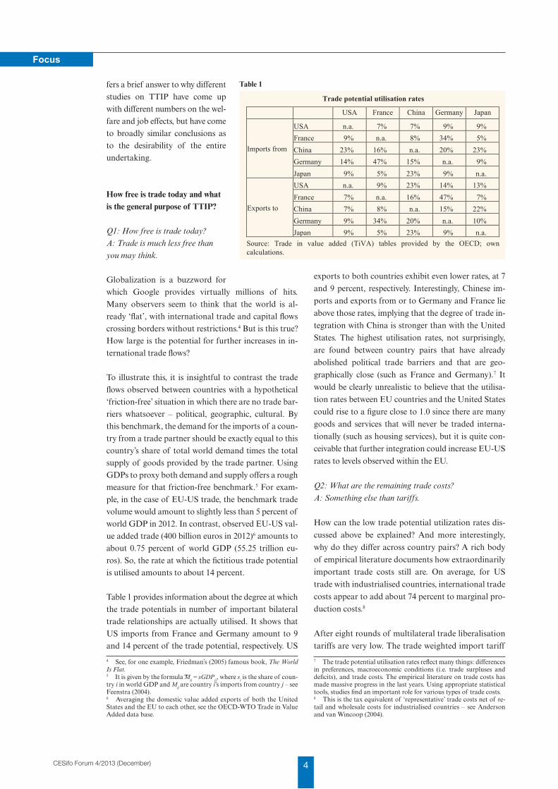
Table 1 provides information about the degree at which the trade potentials in number of important bilateral trade relationships are actually utilised. It shows that US imports from France and Germany amount to 9 and 14 percent of the trade potential, respectively. US

4 See, for one example, Friedman’s (2005) famous book, The World Is Flat.5 It is given by the formula ͠Mij = sGDPji, where si is the share of coun-try i in world GDP and Mij are country i’s imports from country j – see Feenstra (2004).6 Averaging the domestic value added exports of both the United States and the EU to each other, see the OECD-WTO Trade in Value Added data base.

exports to both countries exhibit even lower rates, at 7

and 9 percent, respectively. Interestingly, Chinese im-

ports and exports from or to Germany and France lie

above those rates, implying that the degree of trade in-

tegration with China is stronger than with the United

States. The highest utilisation rates, not surprisingly,

are found between country pairs that have already

abolished political trade barriers and that are geo-

graphically close (such as France and Germany).7 It

would be clearly unrealistic to believe that the utilisa-

tion rates between EU countries and the United States

could rise to a figure close to 1.0 since there are many

goods and services that will never be traded interna-

tionally (such as housing services), but it is quite con-

ceivable that further integration could increase EU-US

rates to levels observed within the EU.

Q2: What are the remaining trade costs?

A: Something else than tariffs.

How can the low trade potential utilization rates dis-

cussed above be explained? And more interestingly,

why do they differ across country pairs? A rich body

of empirical literature documents how extraordinarily

important trade costs still are. On average, for US

trade with industrialised countries, international trade

costs appear to add about 74 percent to marginal pro-

duction costs.8

After eight rounds of multilateral trade liberalisation

tariffs are very low. The trade weighted import tariff

7 The trade potential utilisation rates reflect many things: differences in preferences, macroeconomic conditions (i.e. trade surpluses and deficits), and trade costs. The empirical literature on trade costs has made massive progress in the last years. Using appropriate statistical tools, studies find an important role for various types of trade costs.8 This is the tax equivalent of ‘representative’ trade costs net of re-tail and wholesale costs for industrialised countries – see Anderson and van Wincoop (2004).

Table 1  

Trade potential utilisation rates

USA France China Germany Japan

Imports from

USA n.a. 7% 7% 9% 9% France 9% n.a. 8% 34% 5% China 23% 16% n.a. 20% 23% Germany 14% 47% 15% n.a. 9% Japan 9% 5% 23% 9% n.a.

Exports to

USA n.a. 9% 23% 14% 13% France 7% n.a. 16% 47% 7% China 7% 8% n.a. 15% 22% Germany 9% 34% 20% n.a. 10% Japan 9% 5% 23% 9% n.a.

Source: Trade in value added (TiVA) tables provided by the OECD; own calculations.

Table 1

5 CESifo Forum 4/2013 (December)

Focus

of the EU and the United States relative to the

159  member countries of the WTO (World Trade

Organisation) amounts to less than 3 percent for in-

dustrialised goods and only marginally more for agri-

cultural goods. It follows that the bulk of trade costs

must consist of non-tariff barriers. Besides politically

induced trade barriers, these costs reflect the costs of

transportation and insurance, currency exchange, in-

formation, translation, legal, testing services etc.

Politically induced non-tariff barriers typically arise

from differences in regulatory requirements between

two countries. For example, norms and standards

that need to be met for regulatory approval can be dif-

ferent or even mutually inconsistent, meaning that ex-

pensive product changes are required if a good is to

be sold in a foreign market.

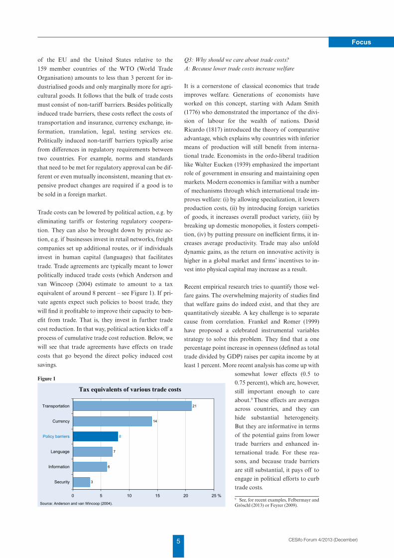
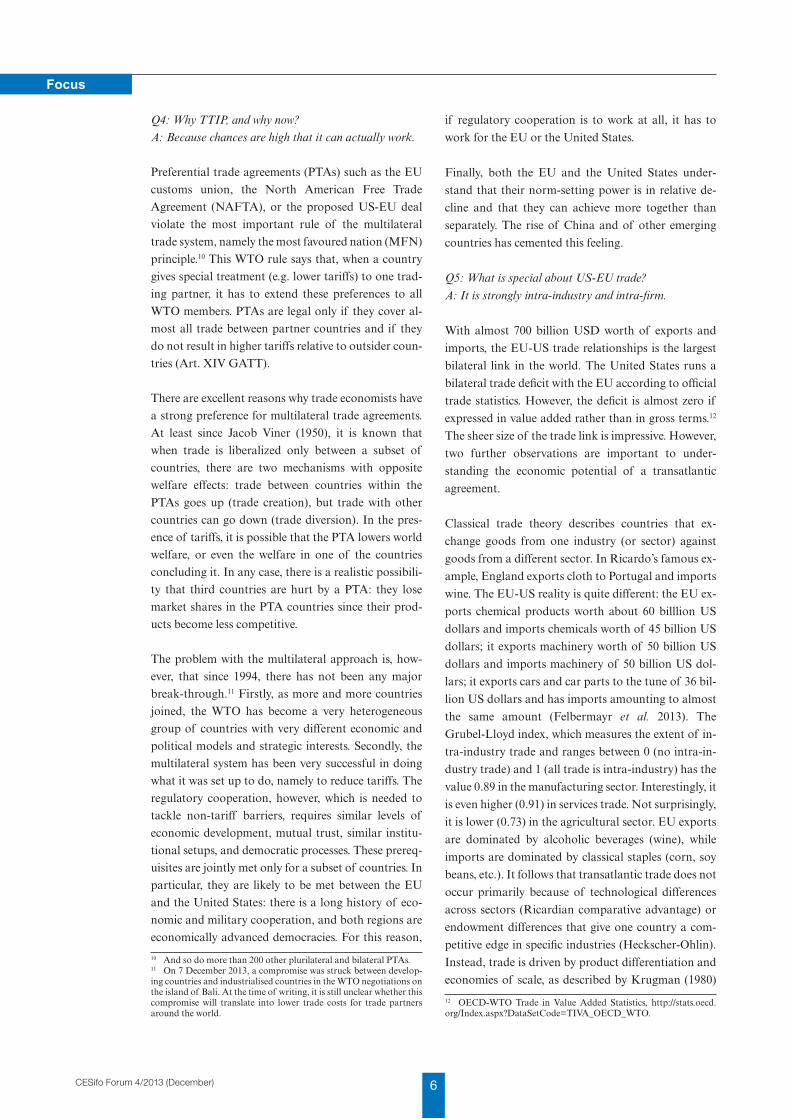
Trade costs can be lowered by political action, e.g. by

eliminating tariffs or fostering regulatory coopera-

tion. They can also be brought down by private ac-

tion, e.g. if businesses invest in retail networks, freight

companies set up additional routes, or if individuals

invest in human capital (languages) that facilitates

trade. Trade agreements are typically meant to lower

politically induced trade costs (which Anderson and

van Wincoop (2004) estimate to amount to a tax

equivalent of around 8 percent – see Figure 1). If pri-

vate agents expect such policies to boost trade, they

will find it profitable to improve their capacity to ben-

efit from trade. That is, they invest in further trade

cost reduction. In that way, political action kicks off a

process of cumulative trade cost reduction. Below, we

will see that trade agreements have effects on trade

costs that go beyond the direct policy induced cost

savings.

Q3: Why should we care about trade costs?

A: Because lower trade costs increase welfare

It is a cornerstone of classical economics that trade

improves welfare. Generations of economists have

worked on this concept, starting with Adam Smith

(1776) who demonstrated the importance of the divi-

sion of labour for the wealth of nations. David

Ricardo (1817) introduced the theory of comparative

advantage, which explains why countries with inferior

means of production will still benefit from interna-

tional trade. Economists in the ordo-liberal tradition

like Walter Eucken (1939) emphasized the important

role of government in ensuring and maintaining open

markets. Modern economics is familiar with a number

of mechanisms through which international trade im-

proves welfare: (i) by allowing specialization, it lowers

production costs, (ii) by introducing foreign varieties

of goods, it increases overall product variety, (iii) by

breaking up domestic monopolies, it fosters competi-

tion, (iv) by putting pressure on inefficient firms, it in-

creases average productivity. Trade may also unfold

dynamic gains, as the return on innovative activity is

higher in a global market and firms’ incentives to in-

vest into physical capital may increase as a result.

Recent empirical research tries to quantify those wel-

fare gains. The overwhelming majority of studies find

that welfare gains do indeed exist, and that they are

quantitatively sizeable. A key challenge is to separate

cause from correlation. Frankel and Romer (1999)

have proposed a celebrated instrumental variables

strategy to solve this problem. They find that a one

percentage point increase in openness (defined as total

trade divided by GDP) raises per capita income by at

least 1 percent. More recent analysis has come up with

somewhat lower effects (0.5 to

0.75 percent), which are, however,

still important enough to care

about.9 These effects are averages

across countries, and they can

hide substantial heterogeneity.

But they are informative in terms

of the potential gains from lower

trade barriers and enhanced in-

ternational trade. For these rea-

sons, and because trade barriers

are still substantial, it pays off to

engage in political efforts to curb

trade costs.

9 See, for recent examples, Felbermayr and Gröschl (2013) or Feyrer (2009).

3

6

7

8

14

21

0 5 10 15 20 25 %

Security

Information

Language

Policy barriers

Currency

Transportation

Tax equivalents of various trade costs

Source: Anderson and van Wincoop (2004).

Figure 1

6CESifo Forum 4/2013 (December)

Focus

Q4: Why TTIP, and why now?

A: Because chances are high that it can actually work.

Preferential trade agreements (PTAs) such as the EU

customs union, the North American Free Trade

Agreement (NAFTA), or the proposed US-EU deal

violate the most important rule of the multilateral

trade system, namely the most favoured nation (MFN)

principle.10 This WTO rule says that, when a country

gives special treatment (e.g. lower tariffs) to one trad-

ing partner, it has to extend these preferences to all

WTO members. PTAs are legal only if they cover al-

most all trade between partner countries and if they

do not result in higher tariffs relative to outsider coun-

tries (Art. XIV GATT).

There are excellent reasons why trade economists have

a strong preference for multilateral trade agreements.

At least since Jacob Viner (1950), it is known that

when trade is liberalized only between a subset of

countries, there are two mechanisms with opposite

welfare effects: trade between countries within the

PTAs goes up (trade creation), but trade with other

countries can go down (trade diversion). In the pres-

ence of tariffs, it is possible that the PTA lowers world

welfare, or even the welfare in one of the countries

concluding it. In any case, there is a realistic possibili-

ty that third countries are hurt by a PTA: they lose

market shares in the PTA countries since their prod-

ucts become less competitive.

The problem with the multilateral approach is, how-

ever, that since 1994, there has not been any major

break-through.11 Firstly, as more and more countries

joined, the WTO has become a very heterogeneous

group of countries with very different economic and

political models and strategic interests. Secondly, the

multilateral system has been very successful in doing

what it was set up to do, namely to reduce tariffs. The

regulatory cooperation, however, which is needed to

tackle non-tariff barriers, requires similar levels of

economic development, mutual trust, similar institu-

tional setups, and democratic processes. These prereq-

uisites are jointly met only for a subset of countries. In

particular, they are likely to be met between the EU

and the United States: there is a long history of eco-

nomic and military cooperation, and both regions are

economically advanced democracies. For this reason,

10 And so do more than 200 other plurilateral and bilateral PTAs.11 On 7 December 2013, a compromise was struck between develop-ing countries and industrialised countries in the WTO negotiations on the island of Bali. At the time of writing, it is still unclear whether this compromise will translate into lower trade costs for trade partners around the world.

if regulatory cooperation is to work at all, it has to

work for the EU or the United States.

Finally, both the EU and the United States under-

stand that their norm-setting power is in relative de-

cline and that they can achieve more together than

separately. The rise of China and of other emerging

countries has cemented this feeling.

Q5: What is special about US-EU trade?

A: It is strongly intra-industry and intra-firm.

With almost 700 billion USD worth of exports and

imports, the EU-US trade relationships is the largest

bilateral link in the world. The United States runs a

bilateral trade deficit with the EU according to official

trade statistics. However, the deficit is almost zero if

expressed in value added rather than in gross terms.12

The sheer size of the trade link is impressive. However,

two further observations are important to under-

standing the economic potential of a transatlantic

agreement.

Classical trade theory describes countries that ex-

change goods from one industry (or sector) against

goods from a different sector. In Ricardo’s famous ex-

ample, England exports cloth to Portugal and imports

wine. The EU-US reality is quite different: the EU ex-

ports chemical products worth about 60 billlion US

dollars and imports chemicals worth of 45 billion US

dollars; it exports machinery worth of 50 billion US

dollars and imports machinery of 50 billion US dol-

lars; it exports cars and car parts to the tune of 36 bil-

lion US dollars and has imports amounting to almost

the same amount (Felbermayr et al. 2013). The

Grubel-Lloyd index, which measures the extent of in-

tra-industry trade and ranges between 0 (no intra-in-

dustry trade) and 1 (all trade is intra-industry) has the

value 0.89 in the manufacturing sector. Interestingly, it

is even higher (0.91) in services trade. Not surprisingly,

it is lower (0.73) in the agricultural sector. EU exports

are dominated by alcoholic beverages (wine), while

imports are dominated by classical staples (corn, soy

beans, etc.). It follows that transatlantic trade does not

occur primarily because of technological differences

across sectors (Ricardian comparative advantage) or

endowment differences that give one country a com-

petitive edge in specific industries (Heckscher-Ohlin).

Instead, trade is driven by product differentiation and

economies of scale, as described by Krugman (1980)

12 OECD-WTO Trade in Value Added Statistics, http://stats.oecd.org/Index.aspx?DataSetCode=TIVA_OECD_WTO.

7 CESifo Forum 4/2013 (December)

Focus

in his Nobel Prize winning work. Those circumstances

have implications, amongst other things, for the na-

ture of the gains from trade and for the effect of trade

on economic inequality.

A second important factor in EU-US trade is that a

large share of trade takes place within multinational

firms. This pattern is particularly strong for US ex-

ports. For example, about 80 percent of US exports in

the automotive industry take place within firms such

as General Motors or Ford. That figure is 40 percent

for EU exports. In the chemical industry the share of

intra-firm trade is about 75 percent for US exports

and 55 percent for EU exports. The importance of

trade within firms reflects the large mutual stock of

foreign direct investment (FDI): many EU firms pro-

duce in the United States and many US firms produce

in the United States. Most FDI between the United

States and the EU is horizontal, since production cost

differences are relatively low compared to other desti-

nations of FDI. The large FDI stocks therefore reflect

high trade costs between the two regions: firms wish to

avoid tariffs or exchange rate risk (e.g. in the automo-

tive industry), or costly transportation (such as in the

chemical industry).

What can we learn from existing preferential trade agreements?

Q6: Do PTAs really increase their members’ trade?

A: Yes. Big time.

There is a large body of empirical literature that inves-

tigates the effects of PTAs on trade flows.13 One of the

big challenges in the empirical quantification of the ef-

fects of PTAs on trade flows lies in the fact that only

countries expecting to gain a lot from an agreement

are likely to sign one. For example, theoretical work

suggests that country size and distance between coun-

tries are important explanatory factors for PTA mem-

bership (see the seminal paper by Baier and Bergstrand

2004). Assuming PTA membership to be exogenous

(i.e., randomly assigned to countries) will therefore

lead to biased estimates of the trade effects of PTAs.

But will this bias be severe?

Some recent papers have given serious consideration

to the endogeneity of PTAs. Trefler (1993), for in-

13 For early contributions, see Tinbergen (1962); Glejser (1968); and Aitken (1973). For some more recent examples, see Freund (2000); Soloaga and Winters (2001); and Carrère (2006), and for a survey, Greenaway and Milner (2002).

stance, investigates the effect of non-tariff barriers on

US multinational imports. Taking into account the

simultaneity of imports and non-tariff barriers, he

concludes that NTBs decrease imports by 24 percent,

a ten-fold increase compared to estimates taking non-

tariff barriers to be exogenous. Baier and Bergstrand

(2002) use treatment estimators to evaluate the effect

of FTAs on trade flows and find that, on average,

when acknowledging the endogeneity of an FTA, the

agreement tends to increase the value of trade by 92

percent.14 Baier and Bergstrand (2007) use panel esti-

mators to control for the potential endogeneity of

PTAs and show that taking into account the potential

endogeneity of PTAs substantially magnifies the esti-

mated effects of trade flows. The point estimates imply

that an FTA will, on average, increase two member

countries’ trade about 100 percent after 10 years,

which is seven times the 14 percent increase effect esti-

mated when neglecting the endogeneity problem.

Baier and Bergstrand (2009) confirm these findings

using a matching estimator. Magee (2003) finds effects

that are even higher, ranging up to 800 percent.

Q7: How do PTAs increase trade?

A: Through lower non-tariff trade barriers.

Given these empirical findings, one may wonder where

these big effects come from. As we have seen above,

the effects cannot be explained by tariff elimination,

as tariff levels are already very low. The more promis-

ing answer is that PTAs must be successful in bringing

non-tariff trade barriers down. However, available

measures of non-tariff measures are very incomplete

and do not capture all products.15 Hence, the existing

quantitative proxies of non-tariff barriers are also not

able to explain the huge potential effects of PTAs.

Potentially, improved estimates of NTBs may explain

the huge effects. Indeed, one could interpret the large

PTA estimates as evidence for substantial non-tariff

barriers to trade. Felbermayr et al. (2013) used such

an approach when evaluating TTIP, taking the ob-

served PTAs up to 2005 and netting out the tariff re-

duction effects of the PTAs. Importantly, such an ap-

proach also accounts for public and private invest-

ment initiatives that also cut trade costs by, for exam-

ple, improving transport infrastructure, deepening

14 They also report results for specific agreements. They report aver-age trade increases for member countries of The Andean Pact of 326 percent, of 395 percent for member countries of the Central American Common Market (CACM), and of 222 percent for membership of MERCOSUR. NAFTA is estimated to increase trade by 86 percent (on average) among Canada, Mexico, and the United States.15 See Anderson and van Wincoop (2004) for an excellent discussion.

8CESifo Forum 4/2013 (December)

Focus

currency markets, extending business networks, or lowering language barriers.

Yet another explanation for the large effects could be the complementarity between goods trade liberaliza-tion and other liberalizations, such as liberalization of investment and services trade. Egger, Larch and Staub (2012) are one example of authors who study the in-terrelationship of goods and services trade and trade agreements. One of their main findings is that changes in goods preferences via a goods trade agreement not only affect goods trade, but also services trade. The employed model leads to lower gains in goods and ser-vice trade agreements for the average economy than a one-sector goods-only model. If liberalization takes place in one sector only, focusing on a single sector economy may bias calculated trade and welfare effects upward by attributing activity (GDP and employ-ment) in the non-liberalized sector to the liberalized sector. Hence, accounting for the interaction of goods and services trade may explain part of the large ob-served trade agreement effects.

Q8: Do PTAs divert trade? A: They typically do.

Panagariya (2000) nicely motivates his discussion of trade diversion and creation by stating: “any discus-sion of the welfare effects of PTAs must inevitably be-gin with the influential concepts of trade creation and diversion”. Are these trade diversion effects substantial?16 While Clausing (2001) finds little evi-dence for trade diversion for the Canada – United States Free Trade Agreement (CUSFTA),17 Trefler (2004) and Romalis (2007) do find evidence for trade diversion for CUSFTA and NAFTA, respectively. Whereas Trefler (2004) finds trade creation does still outweigh trade diversion to ensure that there are wel-fare gains from NAFTA in Canada, Romalis (2007, 417) concludes that “the more detailed data used in this paper reveals much more substantial trade diver-sion than Trefler, so much so that there appear to be essentially no welfare gains for any NAFTA mem-ber”. However, Romalis (2007) does not only find no welfare gains for the NAFTA members, but also finds evidence for negative third-country effects for non-NAFTA members. His analysis of trade diversion re-veals that a 1 percent drop in intra-North American

16 Panagariya (1999) is a nice survey discussing the likely effects of PTAs, including potential trade diversion effects.17 Note that Clausing (2001) uses prices rather than quantities in the welfare analysis, which is problematic (see Feenstra 2004). Additionally, the results from Clausing (2001) may be driven by the rapid growth of imports that would have occurred if CUSFTA had not have been in place – see Romalis (2007).

tariffs leads to about a 2 percent fall in exports from

other countries relative to the EU.

Chang and Winters (2001) analyses the trade diver-

sion effects of non-MERCOSUR exports to Brazil af-

ter the inception of MERCOSUR. They find strong

negative terms-of-trade effects for non-member coun-

tries and conclude their analysis with the statement:

“our results give empirical backing to the well-known

theoretical argument that even if external tariffs are

unchanged by integration, non-member countries are

likely to be hurt by regional integration” (Chang and

Winters 2001, 901).

Q9: Is regulatory cooperation within a PTA trade

diverting? A: Most likely, yes.

Regulatory cooperation can proceed in two main

ways: by creating a joint standard, or by mutually rec-

ognising standards. Establishing joint standards is

hard, so most progress has been made by negotiating

mutual recognition agreements (MRAs). The problem

with MRAs is that they do not create a single world

standard to which third countries can adhere. Instead,

these countries would have to abide by the national

standards in the PTA countries, since the MRA does

not extend to them. For this reason, MRAs are poten-

tially equally as trade diverting as tariff reductions;

joint standards, in contrast, could actually spur third

country trade. What is the empirical evidence on this

question?18

Chen and Mattoo (2008) use panel data to analyse

the effects of PTAs that harmonise standards and

find that while they increase trade between partici-

pating countries, the effects on outsiders are less

clearly cut. They depend on the ability of the outside

countries to meet standards. As the standards are

more likely to be met by developed than by develop-

ing countries, Chen and Mattoo (2008) conclude that

developing countries in particular will be negatively

affected by trade diversion from an MRA where they

are not a member. Additionally, the stringency of the

rules of origin plays a crucial role for the effects on

outsiders. If the rules of origin are very strict, then

gains from the MRA are restricted to MRA member

countries, whereas if they are not, outside countries

also potentially stand to gain from the harmonisa-

tion of standards of other countries. Baller (2007)

uses a gravity model accounting for heterogeneous

18 For a detailed discussion, see the World Trade Report (2012) pre-pared by the WTO.

9 CESifo Forum 4/2013 (December)

Focus

firms to investigate the effects of MRAs on devel-

oped and developing countries. She distinguishes be-

tween MRAs for which she finds positive effects on

the extensive (entering new markets) and intensive

(volume of trade) margin, and harmonisation of

standards or technical regulations. For the latter she

finds ambiguous effects. Specifically, in line with

Chen and Mattoo (2008), she finds that developing

countries’ trade is affected by regional harmonisa-

tion, whereas trade with developed countries is

increased.

Fink and Jansen (2009) focus on services trade and ar-

gue that the scope for MRAs is likely to be limited.

The reason is that with regard to services, MRAs are

mainly relevant for mode 4 movements.19 However,

mode 4 trade is hardly affected by trade liberalization,

making large gains from MRAs unlikely. Furthermore,

MRAs for services only apply to a small number of

professional services sectors, like accounting, architec-

ture and engineering. In addition, most of the MRAs

do not implement the automatic recognition of quali-

fications (OECD 2003), limiting their effect even fur-

ther. There is also a recent paper by Cadot et al. (2013)

that highlights trade diversion effects for non-tariff

measures. The authors show that North-South PTAs

hurt trade between developing countries. If the har-

monisation is based on regional standards, exports of

developing countries to developed countries are also

predicted to be negatively affected.

How will TTIP affect world trade patterns?

Q10: By how much can TTIP potentially lower trade

costs? A: By as much as existing agreements.

Having discussed empirical evidence on existing PTAs,

it is very likely that we would also expect TTIP to lead

to decreases in trade costs between the United States

and the EU. However, TTIP has not been negotiated

yet, so nobody knows exactly what the negotiating

parties will agree upon. For a quantitative assessment

of TTIP’s potential effects, there are two options (i)

make assumptions on how TTIP will change trade

costs, or (ii) take other existing PTAs to infer an aver-

age effect of PTAs that we can use as our best estimate

for the effects of TTIP.

19 Mode 4 movements are services supplied by nationals of one coun-try in the territory of another. This includes independent services sup-pliers and employees of the services supplier of another country, like, for example, a doctor going from his home country to the patients’ country to treat him there.

The second approach is the one undertaken by

Felbermayr et al. (2013). The authors highlight that the

partial (non-general equilibrium effects) of PTAs based

on this approach are around 200 percent on trade flows

when taking into account selection into PTAs as dis-

cussed previously.20 This effect is well in line with the

results of previous studies of the effects of PTAs taking

endogeneity seriously. Depending on the choice of

trade elasticities, such a big effect means that PTAs

must have been able to reduce ad valorem trade costs by

something between 15 and 30 percent.21 While it is un-

clear if the US-EU agreement can achieve as much as

existing treaties, we cannot assess this any more accu-

rately until the negotiations have been concluded.

Q11: How does TTIP affect transatlantic trade? A: It

could almost double it.

In Felbermayr et al. (2013), we use a very standard

general equilibrium trade model to simulate the effects

resulting from lowering trade costs between the

United States and EU countries by exactly the average

reduction observed in the econometric estimates for

existing PTAs. In such a scenario, GDPs of all 126 in-

cluded countries adjust, and so do wages, prices, and

the so called multilateral resistance indices. These var-

iables jointly determine how bilateral trade patterns

adjust. Table 2 shows effects for selected country

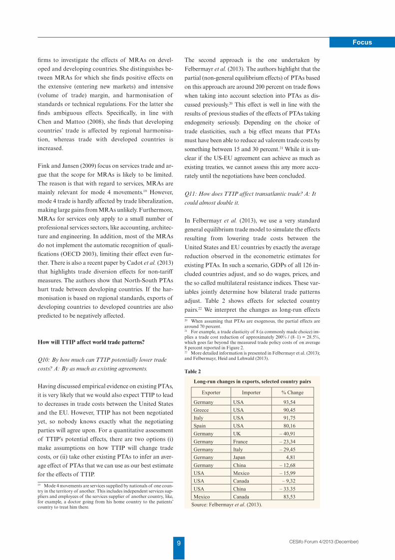
pairs.22 We interpret the changes as long-run effects

20 When assuming that PTAs are exogenous, the partial effects are around 70 percent.21 For example, a trade elasticity of 8 (a commonly made choice) im-plies a trade cost reduction of approximately 200% / (8–1) = 28.5%, which goes far beyond the measured trade policy costs of on average 8 percent reported in Figure 2.22 More detailed information is presented in Felbermayr et al. (2013); and Felbermayr, Heid and Lehwald (2013).

Table 2 Long-run changes in exports, selected country pairs

Exporter Importer % Change

Germany USA 93,54 Greece USA 90,45 Italy USA 91,75 Spain USA 80,16 Germany UK – 40,91 Germany France – 23,34 Germany Italy – 29,45 Germany Japan 4,81 Germany China – 12,68 USA Mexico – 15,99 USA Canada – 9,32 USA China – 33.35 Mexico Canada 83,53

Source: Felbermayr et al. (2013).

Table 2

10CESifo Forum 4/2013 (December)

Focus

since the empirical estimates they are based on refer to

long-run estimates as well (i.e. assuming that all PTA-

related trade cost reduction effects have fully played

out). The table shows that trade (between EU coun-

tries and the United States) goes up by 80 to 90 per-

cent compared to a scenario whereby no TTIP was

signed.

Q12: How does TTIP affect intra-EU trade?

A: It reduces its relative importance.

In the experiment, trade between EU member states

falls by 20 percent to 40 percent. A comprehensive

agreement between the EU and the United States di-

lutes the trade diversion effects that have driven

European trade integration since the creation of the

EU customs union. Without TTIP producers from

Germany are advantaged over producers from the

United States when selling to France, as trade barriers

with France are lower. TTIP undoes the relative ad-

vantage of German firms in France, since American

competitors gain equal access to the French market.

For similar reasons, trade between the United States

and its NAFTA partners Canada and Mexico falls by

10 to 16 percent.

Q13: How does TTIP affect third countries’ trade?

A: There are winners and losers.

Finally, both trade between EU members and the

United States with China falls. However, there is a

great deal of heterogeneity resulting from the general

equilibrium effects taking place: for example, trade be-

tween Japan and Germany can be expected to go up.

Trade between third parties also increases – in some

cases quite substantially, as evidenced by the Canada-

Mexico pairing. It is worth noting that the size of

trade diversion effects is substantial, because both the

EU and the United States are usually amongst the

most important export destinations for most countries

in the world. The EU and the United States each ac-

count for about a quarter of global demand.

Q14: What explains heterogeneity in trade effects?

A: Gravity.

The gravity equation, the workhorse model to explain

bilateral trade, relates bilateral trade flows to GDPs of

countries, bilateral distance, as well as multilateral

trade barriers (see Feenstra (2004) for a textbook

treatment). Hence, the effect of changes in trade costs

induced by PTAs is also shaped by the GDPs of coun-

tries and their geography. Most importantly, trade

barriers lead to larger reductions in trade between

large countries than between small countries

(Implication 1 of Anderson and van Wincoop 2003).

Applied to TTIP, this means that large trade gains are

expected between large countries, as seen in the case

of the United States as a trading partner of the large

EU area, for example. Additionally, more remote

countries with low levels of trade are less affected,

both by positive effects when part of TTIP, and by

negative trade diversion effects when not a member of

TTIP. This can most clearly be seen by the largest

trade diversion effects for countries that are geograph-

ically close to TTIP members, but not themselves

members of TTIP.

Can TTIP increase welfare and create jobs, and for whom?

Q15: How does TTIP affect developed countries’

welfare? A: EU and the United States win. Others lose.

Felbermayr et al. (2013) present a long-term welfare

analysis for 126 countries. On average, they find wel-

fare effects (expressed as equivalent variations) of 3.3

percent in the long-run from a far reaching liberaliza-

tion that not only reduces tariffs, but also abandons

NTBs (measured by past average effects of PTAs).

While the gains in real GDP per capita (their welfare

measure) is calculated to be 4.75 in Germany and 2.6

percent in France, the United States and Britain are

expected to gain substantially more (13.4 percent and

9.7 percent, respectively). Assuming the full trade cost

reducing effects of TTIP to ramp up over 15 years, the

yearly growth impulses from TTIP can be approximat-

ed by dividing the long-run effects by 15.

As discussed before, these gains are very likely to be

accompanied by welfare losses due to trade diversion

from trading partners of TTIP countries that are not

themselves TTIP members. Specifically, we predict

substantial welfare losses for Canada (– 9.5 percent),

Australia (– 7.4 percent), Mexico (– 7.2 percent), and

Japan (– 5.9 percent) as important trading partners of

the United States and the EU. If the EU and the

United States sign trade agreements with these coun-

tries, these negative effects are likely to be much atten-

uated (with the exception of Mexico, with which both

the EU and the United States already have deals.) The

most heavily influenced trading partners of the EU

outside TTIP are Switzerland (– 3.75 percent) and

11 CESifo Forum 4/2013 (December)

Focus

Turkey (– 3.7 percent).23 Amongst the BRICS coun-

tries, South Africa faces the largest losses (– 3.2 per-

cent), Brazil, Russia and India stand to lose about

2  percent, and China remains relatively unaffected

(– 0.4 percent).

Q16: How does TTIP affect the developing world?

A: A few win, more lose.

A couple of papers that highlight the potential nega-

tive effects of PTAs between developed countries for

outside developing countries are cited above. This is

not only the case if the PTA reduces tariffs, but also if

it reduces NTBs. Out of the 126 countries under in-

vestigation in the study of Felbermayr et al. (2013)

many countries are developing

countries. Looking at their re-

sults confirms the findings of pre-

vious empirical studies of sub-

stantial negative effects for devel-

oping countries.

Taking the definition of the

World Bank for low-income

countries, i.e. countries with a

per capita gross national income

23 Turkey is in the peculiar situation that it is in a customs union with the EU. Therefore, it has to implement all concessions that the EU makes to the United States in the pro-cess of concluding TTIP. The United States, in turn, is not required to extend concessions given to the EU to Turkey, as Turkey is not a member of the EU.

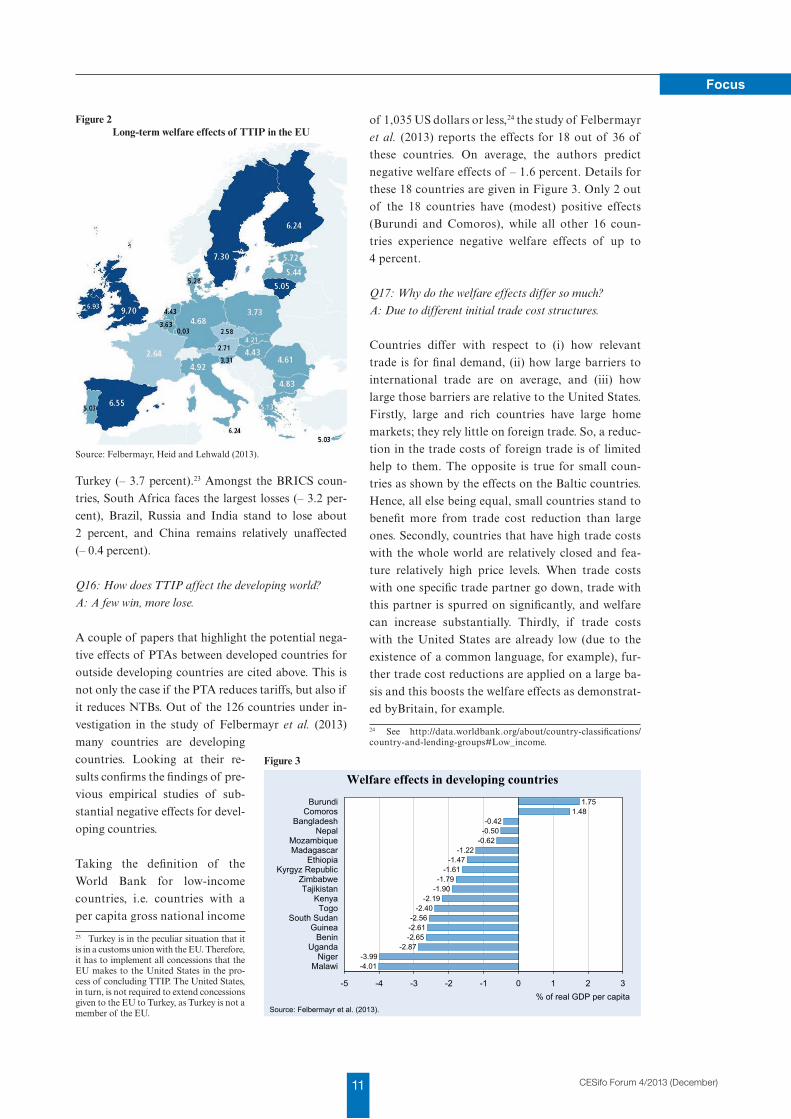
of 1,035 US dollars or less,24 the study of Felbermayr

et al. (2013) reports the effects for 18 out of 36 of

these countries. On average, the authors predict

negative welfare effects of – 1.6 percent. Details for

these 18 countries are given in Figure 3. Only 2 out

of the 18  countries have (modest) positive effects

(Burundi and Comoros), while all other 16 coun-

tries experience negative welfare effects of up to

4 percent.

Q17: Why do the welfare effects differ so much?

A: Due to different initial trade cost structures.

Countries differ with respect to (i) how relevant

trade is for final demand, (ii) how large barriers to

international trade are on average, and (iii) how

large those barriers are relative to the United States.

Firstly, large and rich countries have large home

markets; they rely little on foreign trade. So, a reduc-

tion in the trade costs of foreign trade is of limited

help to them. The opposite is true for small coun-

tries as shown by the effects on the Baltic countries.

Hence, all else being equal, small countries stand to

benefit more from trade cost reduction than large

ones. Secondly, countries that have high trade costs

with the whole world are relatively closed and fea-

ture relatively high price levels. When trade costs

with one specific trade partner go down, trade with

this partner is spurred on significantly, and welfare

can increase substantially. Thirdly, if trade costs

with the United States are already low (due to the

existence of a common language, for example), fur-

ther trade cost reductions are applied on a large ba-

sis and this boosts the welfare effects as demonstrat-

ed byBritain, for example.

24 See http://data.worldbank.org/about/country-classifications/country-and-lending-groups#Low_income.

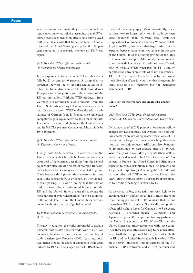
Source: Felbermayr, Heid and Lehwald (2013).

Figure 2 Long-term welfare effects of TTIP in the EU

-4.01-3.99

-2.87-2.65-2.61-2.56

-2.40-2.19

-1.90-1.79

-1.61-1.47

-1.22-0.62

-0.50-0.42

1.481.75

-5 -4 -3 -2 -1 0 1 2 3

MalawiNiger

UgandaBenin

GuineaSouth Sudan

TogoKenya

TajikistanZimbabwe

Kyrgyz RepublicEthiopia

MadagascarMozambique

NepalBangladesh

ComorosBurundi

Welfare effects in developing countries

Source: Felbermayr et al. (2013).

% of real GDP per capita

Figure 3

12CESifo Forum 4/2013 (December)

Focus

Q18: Why are the welfare effects potentially large?

A: Because TTIP would be big and deep.

The United States and the EU together account for

about 45 percent of world GDP (measured in US dol-

lars). A comprehensive reduction in trade costs be-

tween these regions could therefore result in massive

trade and welfare effects. Existing trade flows would

be freed from costly barriers, resulting in resource sav-

ings in the EU and the United States. Tariff reform, by

contrast, does not primarily lead to resource savings.

Tariffs are taxes, so abolishing them implies a loss of

government income (tariff income from trade with the

United States amounts to about 6 billion euros for the

EU in 2012). In the tariff scenario, welfare gains are

‘triangular’ (the famous dead weight loss), while in a

trade cost scenario, they are rectangular.

Moreover, it is important to understand that the simu-

lated trade creation in the United States and Europe is

so strong, precisely because of the existence of diver-

sion effects. This means that the negative welfare ef-

fects obtained in some countries due to the dominance

of trade diversion effects contribute to the positive

welfare gains elsewhere. If one assumes that – contra-

ry to what the data suggest – regulatory reform in

PTAs lowers trade costs around the world, welfare

losses in third countries would be smaller, but so

would be the gains in the PTA countries.

Finally, TTIP occurs in a setup in which many other

PTAs already exist. The most relevant of these PTAs

are the EU customs union and NAFTA. These agree-

ments have presumably led to trade creation between

member states, and to trade diversion with third coun-

tries. The fact that TTIP undoes some of the trade di-

version relative to the EU or the United States acti-

vates welfare gains for the EU or the United States.

Q19: Does TTIP create additional jobs?

A: In the long-run: yes. But few.

The public is understandably concerned by effects of

international trade agreements on jobs. Trade econo-

mists, however, have long argued that dysfunctional la-

bour market institutions, which create excessive unem-

ployment, have to be tackled by labour market reforms.

International trade plays a comparatively small role.

However, the literature on this topic nevertheless pro-

vides insights into a number of important aspects.

Firstly, trade liberalization typically creates winners

and losers: some sectors and firms expand, while oth-

ers shrink; and this requires lay-offs in some places

and job creation in others. In this process of restruc-

turing, trade can increase unemployment in the short-

run. Dutt, Mitra and Ranjan (2009) provide evidence

of this effect. In the context of the TTIP, however, re-

structuring will mostly take place within industries,

not between them, since transatlantic trade is primar-

ily of the intra-industry type. Clearly, intra-industry

reallocation is less costly than inter-industry realloca-

tion, as human capital can be transferred much more

easily between firms in the same sector than between

firms in different sectors.

Secondly, in the long run, trade offers the possibility

of job gains. In labour markets that are prone to

search frictions, lower trade costs lower the costs of

internationally sourced inputs that are complements

to labour and this can encourage firms to create more

jobs. These mechanisms are described in Felbermayr,

Prat and Schmerer (2011a) and their empirical rele-

vance is tested in Felbermayr, Prat and Schmerer

(2011b), as well as in Dutt, Mitra and Ranjan (2009).

Heid and Larch (2012) construct a quantitative trade

model that allows for search unemployment and

which can be implemented in a similar fashion to the

approaches that we have described above. Felbermayr,

Heid and Lehwald (2013) have done so for TTIP and

find that the effects on employment are positive.

Robustness checks carried out in Felbermayr et al.

(2013) and in Felbermayr, Lehwald, Schoof and

Ronge (2013) confirm these findings.

However, these robustness checks also confirm that

job gains are relatively modest. For example, in the

most optimistic scenario, employment increases by

about 200,000 jobs in Germany in the long-run

(15 years). This amounts to less than 0.5 percent of

current employment (about 42 million workers). As

mentioned above, to cure labour market problems,

one needs labour market reforms; trade policy is not

the right tool to apply.

What are TTIP’s effects on social cohesion, the environment and the world trade system?

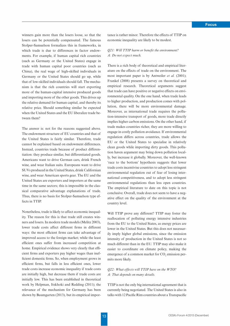
Q20: Will TTIP increase inequality in the participating

countries? A: Possibly; but small effects.

International trade typically creates losers and win-

ners. In the presence of aggregate gains from trade, the

13 CESifo Forum 4/2013 (December)

Focus

winners gain more than the losers loose, so that the

losers can be potentially compensated. The famous

Stolper-Samuelson formalizes this in frameworks, in

which trade is due to differences in factor endow-

ments. For example, if human capital rich countries

(such as Germany or the United States) engage in

trade with human capital poor countries (such as

China), the real wage of high-skilled individuals in

Germany or the United States should go up, while

that of low-skilled individuals should fall. The mecha-

nism is that the rich countries will start exporting

more of the human-capital intensive produced goods

and importing more of the other goods. This drives up

the relative demand for human capital, and thereby its

relative price. Should something similar be expected

when the United States and the EU liberalize trade be-

tween them?

The answer is: not for the reasons suggested above.

The endowment structure of EU countries and that of

the United States is fairly similar. Therefore, trade

cannot be explained based on endowment differences.

Instead, countries trade because of product differen-

tiation: they produce similar, but differentiated goods.

Americans want to drive German cars, drink French

wine, and wear Italian suits. Europeans want to drive

SUVs produced in the United States, drink Californian

wine, and wear American sports gear. The EU and the

United States are exporters and importers at the same

time in the same sectors; this is impossible in the clas-

sical comparative advantage explanations of trade.

Thus, there is no basis for Stolper-Samuelson type ef-

fects in TTIP.

Nonetheless, trade is likely to affect economic inequal-

ity. The reason for this is that trade still creates win-

ners and losers. In modern trade models (Melitz 2003),

lower trade costs affect different firms in different

ways: the most efficient firms can take advantage of

improved access to the foreign market; while the least

efficient ones suffer from increased competition at

home. Empirical evidence shows very clearly that effi-

cient firms and exporters pay higher wages than inef-

ficient domestic firms. So, when employment grows in

efficient firms, but falls in less efficient ones, lower

trade costs increase economic inequality if trade costs

are initially high, but decrease them if trade costs are

initially low. This has been established in theoretical

work by Helpman, Itskhoki and Redding (2011); the

relevance of the mechanism for Germany has been

shown by Baumgarten (2013), but its empirical impor-

tance is rather minor. Therefore the effects of TTIP on

economic inequality are likely to be modest.

Q21: Will TTIP harm or benefit the environment?

A: Do not expect much.

There is a rich body of theoretical and empirical liter-

ature on the effects of trade on the environment. The

most important paper is by Antweiler et al. (2001);

Frankel (2008) presents a survey on theoretical and

empirical research. Theoretical arguments suggest

that trade can have positive or negative effects on envi-

ronmental quality. On the one hand, when trade leads

to higher production, and production comes with pol-

lution, there will be more environmental damage.

Moreover, as international trade requires the pollu-

tion-intensive transport of goods, more trade directly

implies higher carbon emissions. On the other hand, if

trade makes countries richer, they are more willing to

engage in costly pollution avoidance. If environmental

regulation differs across countries, trade allows the

EU or the United States to specialise in relatively

clean goods while importing dirty goods. This pollu-

tion haven argument may bring down pollution local-

ly, but increase it globally. Moreover, the well-known

‘race to the bottom’ hypothesis suggests that lower

trade costs incentivise countries to adopt less stringent

environmental regulation out of fear of losing inter-

national competitiveness, and to adopt less stringent

environmental regulations than less open countries.

The empirical literature to date on this topic is not

conclusive. Overall, trade does not seem to have a neg-

ative effect on the quality of the environment at the

country level.

Will TTIP prove any different? TTIP may foster the

reallocation of polluting energy intensive industries

from the EU to the United States, as energy prices are

lower in the United States. But this does not necessar-

ily imply higher global emissions, since the emission

intensity of production in the United States is not so

much different than in the EU. TTIP may also make it

easier to coordinate on climate policy, making the

emergence of a common market for CO2 emission per-

mits more likely.

Q22: What effects will TTIP have on the WTO?

A: That depends on many details.

TTIP is not the only big international agreement that is

currently being negotiated. The United States is also in

talks with 12 Pacific Rim countries about a Transpacific

14CESifo Forum 4/2013 (December)

Focus

Partnership Agreement (TPP).25 At the same time, the

ten members of the ASEAN26 are negotiating a com-

prehensive economic partnership (RECEP) treaty with

countries (such as China, India or Australia) that al-

ready have PTAs with ASEAN. The emergence of such

big bilateral and plurilateral agreements is very likely

to have an important effect on the multilateral world

trade system and the WTO, since a decreasing share of

world trade will be happening outside of the MFN

discipline.

By the same token, it is possible that new issues arising

in international trade (on labour-related and environ-

mental questions, for instance) will be dealt with not

by the WTO (through future rounds of multilateral

talks, for instance), but within the large plurilateral or

bilateral agreements. So, without much doubt, the role

of the WTO, both as a legislator and as an arbiter, will

become less important. However, TTIP is part of a

more general trend, and cannot be held solely respon-

sible for the WTO’s loss of relevance.

Moreover, the trend towards large PTAs is itself a re-

action to the fact that, due to the depth of the WTO

liberalization process, it has been stuck since 1994,

while the number of WTO members has gone up,

mostly thanks to the addition of emerging econo-

mies.27 The failure to conclude the so-called Doha

Development Round may be at least partly due to the

fact that the WTO membership has become more di-

verse, both in terms of the current and prospective lev-

els of economic development and in terms of political

orientation. While the GATT/WTO system has prov-

en very successful in bringing down trade barriers ‘at

the border’, it seems much less suited to tackling regu-

latory issues ‘behind the border’. Clearly, the mutual

recognition of standards requires a large amount of

trust in the institutional quality of partner countries,

which may not be deep enough in many bilateral rela-

tionships. Moreover, it is unlikely that joint standards

for all WTO members could be optimal. For some

countries such standards will be too stringent, and for

others, too lax, given differences in development sta-

tus. Scepticism as to the capacity and the desirability

of the WTO to deliver significant progress in the area

of NTBs is therefore justified.

25 The TPP negotiations involve the following countries: Australia, Brunei, Chile, Canada, Japan, Malaysia, Mexico, New Zealand, Peru, Singapore, the United States and Vietnam.26 The Association of South-East Asian Nations (ASEAN) was cre-ated in 1967 by Malaysia, the Philippines, Singapore and Thailand and has since been expanded to include Brunei, Burma, Cambodia, Laos and Vietnam.27 The most prominent new members are China (2001), Taiwan (2002), Saudi Arabia (2005), Ukraine (2008), Russia (2012), Vietnam (2007).

All this certainly does not imply that the WTO will

become irrelevant, both as the world trade policeman

and as an engine for further multilateral trade liber-

alization. Firstly, economic theory suggests very

clearly that trade wars (by non-cooperative setting of

tariffs, or standards) yield bigger negative welfare ef-

fects when they take place between large entities than

between small ones – see Felbermayr, Jung and Larch

(2013) for a recent contribution. Thus, the aggrega-

tion of countries into larger entities makes the role of

the WTO as an arbiter even more important.28

Secondly, as we have seen above, large PTAs have sub-

stantial trade diverting effects. Therefore, the emer-

gence of large trade blocs shapes the incentives of all

countries to make concessions in the multilateral pro-

cess. This concerns countries that presently remain

outside of regional megadeals (such as Brazil or

India), but also the EU or the United States, which

are affected by other regional agreements (such as

RCEP). Historical evidence tends to suggest that bi-

lateralism has not hindered progress on the multilat-

eral stage, but may have been complementary to it –

see Baldwin and Jaimovich (2012). A recent example

is provided by the successful negotiation of the so-

called Bali package in December 2013, in which India

made crucial concessions concerning its food subsidy

programs.

Conclusions: an ivory tower wish list for TTIP negotiators

Based on the analysis presented above, and given the

process of on-going negotiations, one may formulate a

number of wishes, which mostly relate to avoiding an

‘economic NATO’ and to creating an open platform

for further multilateral cooperation.

Firstly, it is likely that TTIP will lead to trade diver-

sion. This problem is most pronounced for countries

with which both EU and the United States already

have or are negotiating agreements (e.g. with Canada,

Mexico, Japan and so on). It would be highly desirable

for the bilateral talks between the United States and

the EU to already – without directly involving them –

prepare a path for those countries to sign association

agreements with the TTIP signatories. For example,

this may relate to the handling of rules of origin (cu-

mulation of preferences).

28 This argument is most relevant for customs unions, and neither TTIP, TPP, nor RCEP are designed as such. However, increased regu-latory cooperation (e.g. through common standards) may de facto es-tablish common eternal policies relative to third countries.

15 CESifo Forum 4/2013 (December)

Focus

Secondly, mutual recognition of standards generates

much stronger trade diverting effects than the harmo-

nisation of standards. However, in principle, it is pos-

sible to conceive a cumulation process for standards:

if a third country’s product is assessed as conforming

to either a US or an EU standard, and TTIP includes

a provision on mutual recognition for this product,

then that product should be declared as conforming to

rules in both the EU and the United States without

further assessment.

References

Aitken, N.D. (1973), “The Effect of the EEC and EFTA on European Trade: A Temporal Cross-Section Analysis”, American Economic Review 63, 881–892.

Anderson, J. and E. van Wincoop (2003), “Gravity with Gravitas: A Solution to the Border Puzzle”, American Economic Review 93, 170–192.

Anderson, J. and E. van Wincoop (2004), “Trade Costs”, Journal of Economic Literature 42, 691–751.

Antweiler, W., B. Copeland and M.S. Taylor (2001), “Is Free Trade Good for the Environment?”, American Economic Review 91, 877–908.

Baier, S.L. and J.H. Bergstrand (2002), On the Endogeneity of International Trade Flows and Free Trade Agreements, mimeo.

Baier, S.L. and J.H. Bergstrand (2004), “Economic Determinants of Free Trade Agreements”, Journal of International Economics 64, 29–63.

Baier, S.L. and J. H. Bergstrand (2007), “Do Free Trade Agreements Actually Increase Members’ International Trade?” Journal of International Economics 71, 72–95.

Baier, S.L. and J.H. Bergstrand (2009), “Estimating the Effects of Free Trade Agreements on International Trade Flows Using Matching Econometrics”, Journal of International Economics 77, 63–76.

Baller, S. (2007), Trade Effects of Regional Standards: A Heterogeneous Firms Approach, World Bank Policy Research Working Paper 4124.

Baumgarten, D. (2013), “Exporters and the Rise in Wage Inequality: Evidence from German Linked Employer–Employee Data”, Journal of International Economics 90, 201-217.

Cadot, O., A.-C. Disdier and L. Fontagné (2013), “North-South Standards Harmonization and International Trade”, World Bank Economic Review, forthcoming.

Carrère, C. (2006), “Revisiting the Effects of Regional Trade Agreements on Trade Flows with Proper Specification of the Gravity Model”, European Economic Review 50, 223–247.

Chang, W. and L.A. Winters (2002), “How Regional Blocs Affect Excluded Countries: The Price Effects of MERCOSUR”, American Economic Review 92, 889–904.

Chen, M.X. and A. Mattoo (2008), “Regionalism in Standards: Good or Bad for Trade?”, Canadian Journal of Economics 41, 838–863.

Clausing, K.A. (2001), “Trade Creation and Trade Diversion in the Canada-U.S. Free Trade Agreement”, Canadian Journal of Economics 34, 677–696.

Dutt, P., D. Mitra, and P. Ranjan (2009), “International Trade and Unemployment: Theory and Cross-national Evidence”, Journal of International Economics 78, 32–44.

Egger, H., P. Egger and D. Greenaway (2008), “The Trade Structure Effects of Endogenous Regional Trade Agreements”, Journal of International Economics 74, 278–298.

Egger, P., M. Larch and K. Staub (2012), Trade Preferences and Bilateral Trade in Goods and Services: A Structural Approach, CEPR Working Paper 9051.

Feenstra, R. (2004), Advanced International Trade, Princeton: Princeton University Press.

Felbermayr G., J. Prat and H.-J. Schmerer (2011a), “Globalization and Labor Market Outcomes: Wage Bargaining, Search Frictions, and Firm Heterogeneity”, Journal of Economic Theory 146, 39–73.

Felbermayr G., J. Prat and H.-J. Schmerer (2011b), “Trade and Unemployment: What Do the Data Say?”, European Economic Review 55, 741–758.

Felbermayr, G., M. Larch, L. Flach, E. Yalcin and S. Benz (2013a), Dimensionen und Auswirkungen eines Freihandelsabkommens zwischen der EU und den USA, http://www.cesifo-group.de/ifoHome/research/Projects/Archive/Projects_AH/2013/proj_AH_freihandel_USA-GER.html.

Felbermayr, G., M. Larch, L. Flach, E. Yalcin, S. Benz und F. Krüger (2013b), “Dimensionen und Effekte eines transatlantischen Freihandelsabkommens”, ifo Schnelldienst 66(4), 22–31.

Felbermayr, G. and M. Larch (2013a), “The Transatlantic Trade and Investment Partnership (TTIP): Potentials, Problems and Perspectives”, CESifo Forum 14(2), 49–60.

Felbermayr, G. and M. Larch (2013b), “Das Transatlantische Freihandelsabkommen: Zehn Beobachtungen aus Sicht der Außenhandelslehre”, Wirtschaftspolitische Blätter 60, 353–366.

Felbermayr, G., S. Lehwald and B. Heid (2013), Die Transatlantische Handels und Investitionspartnerschaft (THIP), Studie für die Bertelsmann Stiftung.

Felbermayr, G., S. Lehwald, U. Schoof and M. Ronge (2013), Bundesländer, Branchen und Bildungsgruppen: Wirtschaftliche Folgen eines THIP für Deutschland, Studie für die Bertelsmann Stiftung.

Feyrer, J. (2009), Trade and Income – Exploiting Time Series in Geography, NBER Working Paper 14910.

Felbermayr, G., and J. Gröschl (2013), “Natural Disasters and the Effect of Trade on Income: A New Panel IV Approach”, European Economic Review 58, 18–30.

Fink, C. and M. Jansen (2009), “Services Provisions in Regional Trade Agreements: Stumbling Blocks or Building Blocks for Multilateral Liberalization?”, in: Baldwin, R. E. and P. Low (eds.), Multilateralizing Regionalism: Challenges for the Global Trading System, Cambridge: Cambridge University Press, 221–261.

Fontagné, L., J. Gourdon and S. Jean (2013), Transatlantic Trade: Whither Partnership, Which Economic Consequences?, CEPII Policy Brief 1.

Francois, J., et al. (2013), Reducing Transatlantic Barriers to Trade and Investment: An Economic Assessment, Report for the European Commission.

Frankel, J. (2009), Environmental Effects of International Trade, Expert Report 31, Sweden Globalisation Council.

Freund, C. (2000), “Different Paths to Free Trade: The Gains from Regionalism”, Quarterly Journal of Economics 115, 1317–1341.

Friedman, T.L. (2005), The World Is Flat, New York: Farrar, Strauss and Giroux.

Greenaway, D. and C. Milner (2002), “Regionalism and Gravity”, Scottish Journal of Political Economy 49, 574–585.

Glejser, H. (1968), “An Explanation of Differences in Trade-Product Ratios among Countries”, Cahiers Economiques de Bruxelles 37, 47–58.

Head, K. and T. Mayer (2014), “Gravity Equations: Workhorse, Toolkit, Cookbook”, in: Helpman, E. et al., Handbook of International Economics, Volume IV, forthcoming.

Heid B. and M. Larch (2012), International Trade and Unemployment: A Quantitative Framework, CESifo Working Paper 4013.

16CESifo Forum 4/2013 (December)

Focus

Helpman, E., O. Itskhoki and S. Redding (2010), “Inequality and Unemployment in a Global Economy”, Econometrica 78, 1239–1283.

Jacks, D., C. Meissner and D. Novy (2008), “Trade Costs, 1870–2000”, American Economic Review 98, 529–534.

Krugman, P. (1980), “Scale Economies, Product Differentiation, and the Pattern of Trade”, American Economic Review 70, 950–959.

Magee, C.S. (2003), “Endogenous Preferential Trade Agreements: An Empirical Analysis”, Contributions to Economic Analysis and Policy 2, 1–19.

Melitz, M. (2003), “The Impact of Trade on Intra-Industry Reallocations and Aggregate Industry Productivity”, Econometrica 71, 1695–1725.

OECD (2003), Service Providers on the Move: Mutual Recognition Agreements, TD/TC/WP(2002)48/Final, http://search.oecd.org/of-ficialdocuments/displaydocumentpdf/?doclanguage=en&cote=td/tc/wp(2002)48/final.

Panagariya, A. (1999), “The Regionalism Debate: An Overview”, The World Economy 22, 477–512.

Panagariya, A. (2000), “Preferential Trade Liberalization: The Traditional Theory and New Developments”, Journal of Economic Literature 38, 287–331.

Romalis, J. (2007), “NAFTA’s and CUSFTA’s Impact on International Trade”, Review of Economics and Statistics 89, 416–435.

Soloaga, I. and L.A. Winters (2001), “Regionalism in the Nineties: What Effect on Trade?”, North American Journal of Economics and Finance 12, 1–29.

Tinbergen, J. (1962), Shaping the World Economy, New York: Twentieth Century Fund.

Trefler, D. (1993), “Trade Liberalization and the Theory of Endogenous Protection: An Econometric Study of U.S. import poli-cy”, Journal of Political Economy 101, 138–160.

Trefler, D. (2004), “The Long and Short of the Canada-U.S. Free Trade Agreement”, American Economic Review 94, 870–895.

Viner, J. (1950), The Customs Union Issue, New York: Carnegie Endowment for International Peace.

World Trade Organization (WTO, 2012), World Trade Report 2012 – Trade and Public Policies: A Closer Look at Non-Tariff Measures in the 21st Century, http://www.wto.org/ENGLISH/res_e/reser_e/wtr_e.htm.

AppendixWhy do different studies on TTIP arrive at different conclusions?

The EU Commission has commissioned a study to CEPR (Francois et al. 2013). The Ifo study discussed in this article and the CEPR study come to some simi-lar conclusions, the most important of which is that TTIP is likely to have substantial positive welfare and employment effects in Europe and the United States. There are, however, a number of important differences which derive from (i) differences in the scenario defini-tion, and (ii) differences in methodology. This is not the right place to offer a comprehensive comparison of the studies. In the following, we briefly discuss some of the most relevant differences.

1. The Ifo study adopts a top-down approach on trade costs. In the initial equilibrium, bilateral trade costs are estimated econometrically such that the model replicates the observed trade structure in expecta-tions. The demand structure, in turn, is parameter-ized identically across all country pairs. The CEPR study, in contrast, takes a narrower perspective on trade costs. These are tariffs (as measured in the data), NTBs (estimated outside the model), and transport services. The resulting trade cost struc-ture cannot replicate the observed structure of world trade, so that consumer preferences need to be adjusted. This difference is relevant, because the trade costs are much higher in the Ifo study, and the scope for trade cost reductions is therefore much bigger and potential welfare gains are larger.

2. The Ifo study assumes that TTIP changes the esti-mated trade cost structure for EU-US trade in ex-actly the same way as other PTAs have changed the trade costs for other country pairs. The trade cost reduction derives from tariff elimination and lower non-tariff barriers, but takes into account all other public and private, direct and indirect trade cost re-ducing effects of PTAs. The CEPR study elimi-nates tariffs and lowers the estimated NTBs. Other types of trade costs are not modelled. Moreover, while the Ifo study assumes that NTB reform will benefit only bilateral trade between the EU and the United States, the CEPR study assumes that the EU-US agreement will also lower trade costs multi-laterally through spill-overs. For this reason, the Ifo study predicts major trade diversion effects, and, based on this, larger welfare effects (positive in EU and the United States, mostly negative elsewhere).

17 CESifo Forum 4/2013 (December)

Focus

3. The Ifo study assumes trade costs to be resource

consuming. That is, satisfying foreign standards re-quires costly investment. The CEPR study assumes that NTBs create rents (i.e. income), so that their economic role resembles that of tariffs and has a strong redistributive component (e.g. rents flow from consumers to produces). This assumption greatly reduces the welfare potential of trade reform.

4. The two studies differ with respect to aggregation. The Ifo study models 126 separate countries, but adopts a macroeconomic single-sector perspective. The CEPR study works with 10 regions, but adopts a multi-industry perspective. A more disaggregate geographical perspective allows more precise mod-elling of trade costs. For example, the Ifo study sees the EU as a collection of 28 countries, whose trade is still affected by trade costs. Disregarding within EU trade frictions leads to an overestimation of the EU size of the EU single market, thereby re-ducing the potential gains from bilateral integra-tion with the United States. On the other hand, the rich industry structure of the CEPR model cap-tures that the EU’s and the US’ trade with third parties may happen in different industries than trade between the EU and the United States. This reduces the scope for trade diversion and adverse welfare effects in third countries.

18CESifo Forum 4/2013 (December)

Focus

The TransaTlanTic Trade and invesTmenT ParTnershiP and The shifTing sTrucTure of global Trade Policy

fredrik erixon1

Introduction

Failures in the World Trade Organisation’s Doha Round have prompted countries to turn to preferen-tial trade agreements. Every country with a stake in world trade is now negotiating bilateral free trade agreements – with occasional infusions of regional at-tempts to forge greater trade ties by reducing barriers to trade and investments, e.g. the Trans-Pacific Part-nership (TPP). Some claim that Free Trade Agree-ments (FTAs) are second-best alternatives to a dys-functional multilateral system; while others see them through the eyes of Jacob Viner and consider them to be termites of the trading system, diverting trade and causing bureaucratic obstacles to trade through Rules of Origin regulations.2

Yet regardless the side of the argument, the most out-standing feature of many FTAs is that they do not have impressive effects on growth in trade and GDP. The EU, for instance, considers its FTA in 2011 with South Korea to be a first-of-a-kind, ‘new generation’, ‘deep and comprehensive’ bilateral agreement with a medium-sized growth market – and at the time when it was ratified, EU representatives hailed it as an impor-tant trade agreement for the European post-crisis re-covery. The estimates of the European Commission, however, suggested this FTA to boost GDP in Europe by no more than 0.08 percent (CEPII 2010).

Yet some countries may now be about to enter a new era of preferential trade agreements – an era defined

1 European Centre for International Political Economy (ECIPE), Brussels.2 Bhagwati (2008) offers robust arguments against preferential trade agree ments. My colleague Razeen Sally is also a notable sceptic of many FTAs, especially Asian FTAs – see Sally (2006 and 2007).

by larger preferential trade agreements with more size-

able effects on economic growth and that are premised

on the ambition to usher global trade into the 21st cen-

tury by addressing trade barriers other than those cov-

ered by past WTO agreements. TPP is such an agree-

ment – perhaps the most important trade negotiation

that the United States is currently involved in. Now

that Japan has joined the Trans-Pacific Partnership

negotiations, the value of a TPP deal has risen signifi-

cantly for all countries involved, including the United

States.

The European Union has just launched trade negotia-

tions with Japan. Even if some observers seriously

doubt whether this agreement will materialise, the po-

tential benefits are sizeable and exceed any other bilat-

eral trade agreement that the EU has signed with a

third country. Yet more significantly, the EU and the

United States have now started negotiations for a

Transatlantic Trade and Investment Partnership

(TTIP). If all of these three initiatives yield results,

they will have a serious impact on trade and GDP.

The transatlantic initiative is premised on the idea that

it will extend the scope of a Free Trade Agreement be-

yond the traditional components of eliminating most

tariffs and free up some restrictions on trade in ser-

vices. Agreements to reduce regulatory divergence,

most probably by new horizontal rules and sectoral

agreements like Mutual Recognition Agreements, will

represent the biggest component of TTIP. Further-

more, it will involve an investment component to sub-

stitute current Bilateral Investment Treaties and to

provide for new market access for investments. It will

delve into other ‘unfinished business’ in trade policy,

like openness in public procurement. And leaders on

both sides claim that the agreement should serve as a

platform for cooperating on discrete trade issues glob-

ally, such as competitive neutrality and state-owned

enterprises.

However, TTIP and some of these ambitions are met

with scepticism by some seasoned observers of trade

policy – see, for example, Barfield (2013) and Lang-

hammer (2013). Others, with less careful views, have

also made sceptical contributions to the debate. Have

19 CESifo Forum 4/2013 (December)

Focus

the EU and the United States not tried this before –

and without success – complain some observers? Is

this not just an attempt to create a ‘Fortress Atlantic’

as a defense against competition from rising Asia, es-

pecially China? Another attacking point is that this

initiative is quite typical for the Western-centric ap-

proach to international economic cooperation: just as

other countries are rising to a position of economic

power that could match the EU or the United States,

the old Western powers take their business out of mul-

tilateral organisations to settle affairs bilaterally.

So, is the strange acronym of TTIP a code word for

the death knell of the WTO and multilateral trade co-

operation? Is this a trade agreement premised on de-

fensive attitudes to world trade?

My answer to both questions is ‘No’. Inarguably, there

are some problematic aspects associated with TTIP, as

well as with other large regional agreements, that will

need attention. It should also be acknowledged that

neither TTIP nor TPP was born out of deep and genu-

ine beliefs in the principles of free markets or the clas-

sical school of free trade. Like any other trade agree-

ment in the past years, these initiatives build on con-

ditional views of free trade and free competition,

mixed up with soft mercantilism, a growing urgency

for transatlantic trade leadership, and a pragmatic de-

sire to support economic growth. There are supporters

of TTIP that build their case on more defensive argu-

ments, but to the extent that it is possible to determine

the sentiments that have guided leaders to launch

TTIP, defensive motivations have not been one of

them.

The conclusion of this paper is that countries outside

the EU and the United States, especially the larger

emerging economies, should fear TTIP failure rather

than TTIP success. A failed effort would not only im-

ply less market openness, but probably also less will-

ingness on the part of the two giants of the world

economy to exercise leadership for the world trading

system. The alternative to TTIP is not renewed efforts

to negotiate new multilateral agreements. It follows,

therefore, that my view on TTIP is that it is neither an

attempt at a transatlantic fortress nor an exclusive,

old-club arrangement that will undermine the World

Trade Organisation. If it works well, TTIP is instead

one of few feasible strategies to breathe new life into

international trade cooperation and advance the

agenda for freer trade elsewhere. It is a trade agree-

ment that principally should be feared by those forces

that wish to prevent or deter liberalising trade reforms.

Why TTIP?

The origin of TTIP, at least from the viewpoint of the European Union, is indicative of current trends in European cooperation. Leading voices in the Euro-pean Commission have long been sceptical of transat-lantic trade agreement. The Commission’s Trade Di-rectorate nodded in this direction under the leadership of Leon Brittan – but most of the time the Commis-sion’s view has been that a transatlantic Free Trade Agreement would erode the multilateral system and prevent the EU from negotiation other, and better, trade agreements.

In Europe, TTIP was born out of initiatives taken by member states, especially Germany and Sweden, and the European Parliament.3 And they, along with other participants, managed to persuade a reluctant Com- mission that TTIP would make economic sense and that it would not have damaging consequences on the multilateral system.

There is one argument in particular that has carried weight in Europe’s process to favour a transatlantic trade initiative: the European Union needs higher eco-nomic growth. As a result, trade agreements that could deliver higher economic growth have been given a new hearing as the economic crisis in Europe has worsened. Few would deny that TTIP has the capacity to deliver a sizeable contribution to GDP in Europe. Gains from this FTA would be bigger than from other FTAs for the reason that it involves two large econo-mies. Estimates from a study commissioned by the European Commission suggest that the TTIP gain for the EU would be around 0.3–0.5 percent of GDP (the GDP gains are slightly smaller for the United States) – see Francois et al. (2013). Other estimates suggest that the potential gains may be larger (Felbermayr and Larch 2013) – and some trade economists in Europe have questioned the methodologies used in different studies.4 Yet the ‘official’ estimate still sug-gests that TTIP will have a non-trivial impact on GDP in Europe: GDP should expand by approximately

3 Germany has championed the idea of a transatlantic free trade agreement for several years. Under Germany’s EU Presidency in 2007 it flouted the idea of starting such negotiations – and as part of that strategy initialled the Transatlantic Economic Council. 4 The Commission recently felt compelled to issue an ‘explanatory statement’ regarding the estimates from the study it commissioned, partly to respond to claims that this study had underestimated poten-tial gains (see European Commission 2013).

20CESifo Forum 4/2013 (December)

Focus

120 billion euros, translating into a gain for the aver-

age four-person household of about 550 euros per

year. It is rare that the results of policy achievements

by EU institutions are of that calibre. Consequently,

even under the conservative assumptions used in the

Com mission-led study, TTIP will make a contribution

to economic growth and jobs in the EU that is high

enough to motivate the effort involved in negotiating

TTIP.

The economic case for TTIP is not the only argument

used by leaders of the European Union, or the United

States. But it is the most important one. Other senti-

ments may have some influence too, but only on the

margins. Hillary Clinton portrayed a transatlantic

FTA as an ‘economic NATO’, but trade officials in the

United States acknowledged at an early stage in the

consideration of TTIP that the agreement would be

won or lost for its effects on jobs and growth. Even if

other arguments have not carried the same political

weight, it does not follow that they are less important

analytically.

The ‘sequential strategy’: offensive or defensive?

Arguably, one of the most interesting aspects of TTIP

is its potential effect on global trade – or global efforts

to negotiate new trade agreements. Is this effect posi-

tive or negative – or to put it differently: is it more or

less likely to prompt new and international efforts to

liberalise trade and improve trade rules against dis-

criminatory government action? This section will pre-

sent my view. It is divided in two parts.

Firstly I will address the question of whether TTIP is

a defensive strategy for the European Union – or to

rephrase the question: is TTIP an attempt to avoid

new competition from rising economic powers? The

answer to this question does not only have to rely on

individual judgment: facts and analytical circum-

stances also play a role. The answer to the second

question is much more based on judgement – and that

question is: will TTIP help or hurt efforts to negotiate

new international (potentially multilateral) trade

deals?

There are two arguments against the thesis that TTIP

is a defensive trade strategy.

Firstly, neither the EU nor the United States is solely

focused at their transatlantic initiative. They are both

pursuing trade agendas outside the Atlantic hemi-

sphere. The EU, for instance, is negotiating free trade

agreements with India, Japan, Malaysia, Singapore,

Thailand and Vietnam. It is close to achieving an

agreement with Canada and wants to improve its bi-

lateral trade accord with Mexico, the first NAFTA

country it signed an FTA with. It has a programme for

trade deals in Latin America, and has just gone

through a process of signing off a negotiated deal with

Andean states. It is negotiating a trade agreement with

Mercosur. That negotiation has stalled – but that is

not surprising given the overall course of trade and

economic policy taken by some of the Mercosur

members.

Furthermore, the EU is still trying to get countries in

Africa to agree to Economic Partnership Agreements

that would improve on the one-way market access that

exists through past agreement on preferences. It wants

to have an agreement with the Gulf countries in the

Gulf Cooperation Council. It is now going through a

process of getting a mandate to negotiate a bilateral

investment agreement with China – an agreement that

will also include a market access component. It is hop-

ing to sign an Association Agreement with Ukraine

and is negotiating an agreement aimed at opening up

trade with Eurasia countries through its Eastern

Partnership. It spearheaded Russia’s entry into the

WTO and wants to deepen its trade relations with its

large Eastern neighbour. It is one of the leaders be-

hind the revision of the Information Technology

Agreement (ITA) and the new attempt at negotiating a

plurilateral Trade in Services Agreement (TISA).

The list continues. However, the gist of my point

should be obvious: this is not a trade agenda for an

entity that wants to build a fortress or shield itself

against rising economic powers. Many of these cur-

rent initiatives may not lead to results, or not to the

desired result, but no one should doubt that there is a

grander strategy guiding the EU that is based on lib-

eralising trade with the vast part of the world eco-

nomy.

Trade politics in the United States displays greater un-

easiness about new trade deals, but redrawn ideologi-

cal battle lines in the US Congress should not conflate

the fact that the United States is pushing for several

new trade deals, including TPP and some new plurilat-

eral agreements. The United States no longer consid-

ers itself the hegemon of a global economic system

and has fewer strategic goals associated with its trade

21 CESifo Forum 4/2013 (December)

Focus

policy. Like the European Union, the big shift in US

trade policy over the past decade is that it no longer

accepts trade agreements with only a small degree of

reciprocity. It now demands trade agreements with

two-way trade liberalisation, especially those agree-

ments that involve the large emerging economies that

represent a big part of future demand and trade

growth.

Secondly, if you want to lower your exposure to trade

with some economies, the natural strategy is not to lib-

eralise trade with other economies. In today’s world

economy, it is politically impossible to negotiate trade

agreements that would seriously hurt other important

trade. If TTIP were to have strongly negative conse-

quences on, for instance, EU trade with Asian coun-

tries – if trade diversion were to be sizeable – the net

effect of an agreement would be close to negative.

Such an agreement would be difficult to get accepted

by many players that currently have vested interests in

maintaining current relations with those Asian

countries.

Furthermore, in today’s world economy, the trade-lib-

eralising agreement is not the tool that can be used to

generate serious trade diversion. The effects of bilat-

eral trade agreements on the actual geographical

structures of trade or commercial integration are

small because the preferential effects of tariff reduc-

tions are mostly negligible and because reforms in oth-

er trade policies do not generate much diversion. This

is especially true when two low-tariff economies like

the EU and the United States agree on mutual trade

openings. Real trade diversion tends to be a factor of

the size of an initial tariff and it therefore follows that

the diverting effect of a tariff reduction from, say,

3 percent to zero will have negligible effects.

A bilateral trade agreement between two low-tariff

economies must be focused on effecting trade-prevent-

ing measures that have not been previously addressed

in trade agreements. If such changes can be effected,

they do not divert existing trade to a significant de-

gree. Moreover, some of the changes in market access

cannot be made on a reciprocal and preferential basis:

they tend to apply to other countries too. Let us look

at the effect of TTIP on Sweden, for instance. A sig-

nificant part, approximately two thirds, of the positive

effect of TTIP on GDP will appear in the business ser-

vices sector (one third of the estimated gains will come

from the business services sector) – see National

Board of Trade (2012). This sector has been compara-

tively closed in Sweden and the reforms likely to occur

as a result of TTIP will, in most instances, apply to

other countries too. Changing the rules for commer-

cial presence in, for instance, financial services will

mostly be done on a multilateral basis.

Let us now turn to the second question: will TTIP

help or hurt efforts to negotiate international (possi-

bly multilateral) trade deals? My view – which is based

on my observations rather than undisputed facts – is

that TTIP is more likely to spur on new international

trade deals than to deter them.

The short motivation for this view is based on politics.

The most important factor in changing the political

conditions for new international trade agreements is

that many larger emerging markets become more open

to trade liberalisation, especially countries like China

and India. They are now far too big, and far too im-

portant for actual changes in trade flows generated by

a trade agreement, to be allowed terms of an agree-

ment that would mean little or no liberalisation for

them. An agreement like TTIP will make countries

like China somewhat uncomfortable. They will fear

that they are getting side-lined in discussions over the

structure of future trade agreements. They will feel

compelled to accept trade agreements that they previ-

ously could neglect or even block. This kind of moti-

vation probably played a part in China’s decision to

join the TISA negotiations.

Arguably, this is important to the vitality of the multi-

lateral trading system and to chances to put new glob-

al trade liberalisation firmly on the agenda. Over the

past 15 years, the multilateral trading system has been

a leaderless system with no clear direction that has

unified the key members. The system itself benefited

for several decades from leadership by the United

States, which considered this system to be critical to its

overall strategic objective of spreading market-based

capitalism. There were willing followers to the US

leadership, but none other than the United States had

the requisite economic, political and institutional ca-

pacity to underwrite the system. Yet since the collapse

of the Cold War, American leadership has withered

away, and its general position on trade liberalisation

has changed somewhat. In the absence of political

leadership and direction, the Doha Round got stuck

because the political instinct of many countries was to

favour the status quo, rather than new liberalisation, as

long as there was no external pressure prompting

them to revisit that position.

22CESifo Forum 4/2013 (December)

Focus

Like many other things in economic life, trade liberali-

sation tends to be driven by two motives: profits and

fear. Countries agree to open up to greater foreign

competition because they believe that it will boost

their economy, or because they fear that other coun-

tries will go ahead without them if they stubbornly re-

sist liberalisation. Despite all the success of a trade-

oriented model of growth, many countries have grown

to think that they will not stand to benefit much from

new trade liberalisation, or that the political cost of

liberalisation is too high to stomach.

TTIP may partly change this. It is a big initiative. And

if the two biggest economies of the world go for a bi-

lateral agreement, it means that there is a risk to other

countries that stand outside that bilateral agreement

and, which is important, to other efforts to liberalise

trade. That risk is mostly about not having a voice in

the design of the trade reforms that are likely to serve

as benchmarks in future international agreements. It is

far less about loosing current trade access – but it is

about the fear of not having equally as good access to

trade that will be liberalised in future. Consequently, if

TTIP is the ‘real thing’, if it realises the promise of

ushering the world into 21st century trade policy, the

response from the larger emerging economies cannot

be simply not to respond at all. The political and eco-

nomic opportunity costs of the status quo have

changed.

Concluding comments

It is impossible to say whether TTIP will deliver on its

ambitions. There are several obstacles that stand in

the way of success. Some of the obstacles are political:

a bipartisan US Congress, a US President with a party

divided on trade, political bickering by some EU

member states, etc. Other obstacles are about sub-

stance – and two in particular are critical. Firstly, the

risk that cross-border data portability will be seriously

curtailed by the EU’s new data protection regulation

– and that the EU-US Safe Harbour framework will

be revoked. This risk has, of course, been amplified by

the recent revelations of PRISM and accusations of

large-scale US government surveillance of European

data telecommunication. Secondly, that the EU can-

not agree to change some of its policies derived from

the precautionary principle, especially its policy on

GMOs. Both of these issues need to be addressed if a

deal is to be politically feasible. And the current trend

in policy is one of ever greater distance between the EU and the United States.

References

Barfield, C. (2013), “Not So Fast: Conflicting Deadlines for TPP and the US-EU FTA”, The American, 8 March.

Bhagwati, J. (2008), Termites of the Trading System: How Preferential Trade Agreements Undermine Free Trade, New York: Oxford University Press.

CEPII (2010), The Economic Impact of the Free Trade Agreement between the European Union and Korea, Report for the European Commission.

European Commission (2013), Transatlantic Trade and Investment Partnership: The Economic Analysis Explained, http://trade.ec.europa.eu/doclib/docs/2013/september/tradoc_151787.pdf#Explanatory.

Felbermayr, G. and M. Larch (2013), “The Transatlantic Trade and Investment Partnership (TTIP): Potentials, Problems and Perspectives”, CESifo Forum 14(2), 49–60.

Francois, J. et al. (2013), Reducing Transatlantic Barriers to Trade and Investment: An Economic Assessment, Final Report for the European Commission, London: Centre for Economic Policy Research.

Langhammer, R. (2013), “Transatlantic Free Trade Must Be Achieved Multilaterally Not Bilaterally”, Global Economic Symposium Official Blog, 4 June, http://blog.global-economic-symposium.org/author/rolf- langhammer/.

National Board of Trade (2012), Potential Effects from an EU-US Free Trade Agreement: Sweden in Focus, Stockholm: National Board of Trade.

Sally, R. (2006), FTAs and the Prospects for Regional Economic Integration in Asia, ECIPE Working Paper 1/2006.

Sally, R. (2007), Trade Policy in Asia, ECIPE Policy Briefs 1/2007.

23 CESifo Forum 4/2013 (December)

Focus

Fresh Ideas For a successFul TransaTlanTIc Trade and InvesTmenT ParTnershIP

danIel Ikenson1

Introduction

The potential economic benefits of a comprehensive agreement to liberalize trade, investment, and regula-tory barriers between the United States and the European Union are estimated to be in the range of a total USD100 billion to USD 250 billion annual boost to GDP.2 Realistically, the benefits will depend on whether the enthusiastic rhetoric about achieving a comprehensive agreement is matched by actual ac-complishments on the ground.

An ambitious agreement that lives up to its potential will require resolution of some persistent transatlantic differences across a range of policy issues. Although never easy, on some matters bridging the divides should be fairly straightforward. On others, however, success will require copious amounts of determina-tion, ingenuity, and political will.

To ensure that the TTIP negotiations do not devolve into a decade-long, transatlantic cocktail party, stake-holders will have to hold politicians and negotiators ac-countable to their goals and timetables. Too daunting an enterprise, however, will render success elusive and cause negotiators to lose focus, interest, and, ultimately, the opportunity to achieve meaningful reforms.

In the interest of avoiding that fate, this paper suggests a procedural roadmap for managing the negotiations

1 Cato Institute, Washington DC. This article is a slightly revised version of a paper published by the Cato Institute in October 2013 ti-tled: The Transatlantic Trade and Investment Partnership: A Roadmap for Success.2 Erixon and Bauer (2010) find the annual benefits to be in the range of 117 billion to 168 billion US dollars, Francois et al. (2013) estimate the annual benefits for the EU and the United States at 214  billion euros.

in an orderly, constructive, politically digestible man-

ner. It recommends that:

1. Negotiators identify and announce a discrete set of

specific, achievable goals with realistic deadlines;

2. The negotiations over regulatory processes and

regulatory standards be better defined and made

more manageable by employing a ‘negative list’ ap-

proach, where issues deemed ‘off limits’ to negotia-

tion are specified at the outset so that they do not

obscure the achievable;

3. The negotiators abandon the single undertaking

principle and, instead, aim to produce three succes-

sive biennial agreements by harvesting the lowest

hanging fruit once every two years.

Managing with forethought and determination a pro-

cess that could otherwise descend into an intractable

quagmire is essential to ensuring that negotiators de-

liver most of what they promise.

Towards greater economic integration

The idea of a transatlantic trade agreement has been

floating around for many years, dating back to the

Marshall Plan. There are undoubtedly compelling ra-

tionales for such an agreement, including shared cul-

tural ties, a common history of multilateral institution

building, and similar commitments to democratic

governance.

Moreover, the US and EU economies are already sig-

nificantly integrated. Bilateral trade amounts to about

1 trillion US dollars per year and cross-border direct

investment stocks total 3.7 trillion US dollars.

Bilateral direct investment between the United States

and the European Union constitutes the most inter-

twined, cross-border investment relationship in the

world. Their combined economies account for 34 tril-

lion US dollars in GDP (nearly half of the world’s

output) and more than one-third of all global trade

flows involve the US or EU entities. Reducing barriers

that raise the cost of transatlantic commerce would

generate greater efficiencies and more scope for spe-

24CESifo Forum 4/2013 (December)

Focus

cialization and economies of scale, spawning econom-

ic growth and higher living standards.

But these aren’t new revelations. So, why, after all of

these years of relationship-building, was TTIP for-

mally launched in 2013? Why, after many years of

kicking this idea around and concluding that the ob-

stacles were too daunting, did policymakers suddenly

decide that any impediments were surmountable?

Transatlantic agreement: why now?

As great as the benefits may be, the TTIP was not

borne of any genuine enthusiasm for the enterprise. In

Europe, it was seen as a last resort. Frustrated by the

failures of monetary policy and restricted by the im-

perative of fiscal austerity, policymakers were looking

for something – anything – to embrace as a potential

economic tonic. Whether they actually thought that a

TTIP would be likely to bear fruit is an entirely differ-

ent matter. They wanted something to behold as evi-

dence that Greece did not represent Europe’s fate.

Potential voter wrath, political backlash, and stale-

mate – historically effective deterrents to initiating

transatlantic trade talks – took a back seat to the af-

firmative optics of embracing some plausible initiative

that might steer Europe away from the abyss.

For US policymakers, the main motivation for launch-

ing TTIP was to assuage EU concerns that the United

States had written her off in its ‘pivot’ to Asia.

Other rationales for pursuing TTIP include the argu-

ment that the world needs the United States and the

European Union to reassert global economic leader-

ship at a time when no other country or group of coun-

tries is willing or able to do so. Another is that there is

a race to establish global production standards and

TTIP, representing half the world’s output, presents an

opportunity to establish them here and now. A third

ex-post rationale is that by establishing disciplines on

issues where other trade agreements are silent – issues

like currency manipulation, the operations of state-

owned enterprises, local content rules, and others – the

United States and EU could establish rules that China

and others would eventually have to heed.

It is within this context that TTIP has emerged. But

none of those rationales – pursuing TTIP as a last re-

sort, assuaging hurt feelings, establishing standards,

disciplining China and others – seem likely to provide

the motivation for negotiators and governments to dig

deep and remain committed enough to make difficult

choices that may carry political consequences.

Moreover, in their failures to adequately explain the

enormous benefits that derive from greater freedom to

trade and invest across borders, policymakers on both

sides of the Atlantic have ensured that scepticism

about trade liberalization – and particularly about

agreements with terms that penetrate deeply into do-

mestic regulatory spaces – will persist, rendering the

prospect of a successful TTIP uncertain.

As the talks drag on and opposition mounts, will gov-

ernments remain committed to the goals? Will govern-

ments motivated by the ‘last resort’ rationale continue

to invest seriously in the negotiations if their econo-

mies experience growth and the political costs of TTIP

no longer look so necessary to incur? There have al-

ready been signs of retreat from the ambitious goals

articulated at the outset.

Taking small, digestible bites is the key to TTIP success

From the outset, negotiators erred by setting a 2014

completion date for the negotiations. There is absolute-

ly no plausibility to that deadline and, frankly, a failure

to amend the timetable with realistic deadlines will only

undermine the credibility of the undertaking with a

public that is already sceptical of trade negotiations.

There are dozens of issues on the table of varying

complexity that will probably take several years to re-

solve. Rather than have a single deadline for a single

undertaking, the negotiators should announce that

their intention is to achieve a multi-tiered agreement

that yields multiple harvests at established time inter-

vals. Some analysts have referred to the TTIP as a ‘liv-

ing agreement’, although a common understanding of

that concept is not evident nor, to this writer’s knowl-

edge, have the governments or their negotiators used

this characterization in any official context. They

should; and it should work something like this.

Negotiators would take stock of the issues on the table

and rank them in order of importance to a successful

TTIP conclusion. They would then rank those same is-

sues in terms of order of difficulty to resolve. Based on

averaging and some agreed upon weighting of those

two sets of rankings, negotiators would identify what

they and their counterparts see as the most important

and least important issues, as well as the most difficult

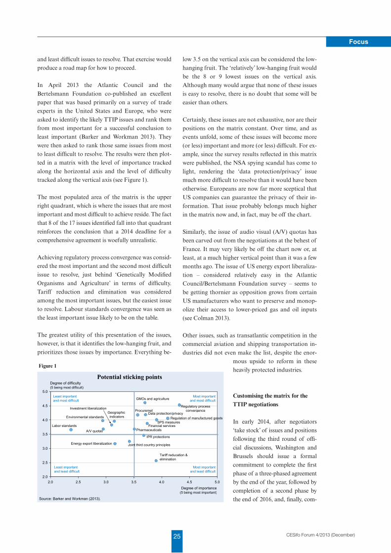
25 CESifo Forum 4/2013 (December)

Focus

and least difficult issues to resolve. That exercise would

produce a road map for how to proceed.

In April 2013 the Atlantic Council and the

Bertelsmann Foundation co-published an excellent

paper that was based primarily on a survey of trade

experts in the United States and Europe, who were

asked to identify the likely TTIP issues and rank them

from most important for a successful conclusion to

least important (Barker and Workman 2013). They

were then asked to rank those same issues from most

to least difficult to resolve. The results were then plot-

ted in a matrix with the level of importance tracked

along the horizontal axis and the level of difficulty

tracked along the vertical axis (see Figure 1).

The most populated area of the matrix is the upper

right quadrant, which is where the issues that are most

important and most difficult to achieve reside. The fact

that 8 of the 17 issues identified fall into that quadrant

reinforces the conclusion that a 2014 deadline for a

comprehensive agreement is woefully unrealistic.

Achieving regulatory process convergence was consid-

ered the most important and the second most difficult

issue to resolve, just behind ‘Genetically Modified

Organisms and Agriculture’ in terms of difficulty.

Tariff reduction and elimination was considered

among the most important issues, but the easiest issue

to resolve. Labour standards convergence was seen as

the least important issue likely to be on the table.

The greatest utility of this presentation of the issues,

however, is that it identifies the low-hanging fruit, and

prioritizes those issues by importance. Everything be-

low 3.5 on the vertical axis can be considered the low-

hanging fruit. The ‘relatively’ low-hanging fruit would

be the 8 or 9 lowest issues on the vertical axis.

Although many would argue that none of these issues

is easy to resolve, there is no doubt that some will be

easier than others.

Certainly, these issues are not exhaustive, nor are their

positions on the matrix constant. Over time, and as

events unfold, some of these issues will become more

(or less) important and more (or less) difficult. For ex-

ample, since the survey results reflected in this matrix

were published, the NSA spying scandal has come to

light, rendering the ‘data protection/privacy’ issue

much more difficult to resolve than it would have been

otherwise. Europeans are now far more sceptical that

US companies can guarantee the privacy of their in-

formation. That issue probably belongs much higher

in the matrix now and, in fact, may be off the chart.

Similarly, the issue of audio visual (A/V) quotas has

been carved out from the negotiations at the behest of

France. It may very likely be off the chart now or, at

least, at a much higher vertical point than it was a few

months ago. The issue of US energy export liberaliza-

tion – considered relatively easy in the Atlantic

Council/Bertelsmann Foundation survey – seems to

be getting thornier as opposition grows from certain

US manufacturers who want to preserve and monop-

olize their access to lower-priced gas and oil inputs

(see Colman 2013).

Other issues, such as transatlantic competition in the

commercial aviation and shipping transportation in-

dustries did not even make the list, despite the enor-

mous upside to reform in these

heavily protected industries.

Customising the matrix for the TTIP negotiations

In early 2014, after negotiators

‘take stock’ of issues and positions

following the third round of offi-

cial discussions, Washington and

Brussels should issue a formal

commitment to complete the first

phase of a three-phased agreement

by the end of the year, followed by

completion of a second phase by

the end of 2016, and, finally, com-

2.0

2.5

3.0

3.5

4.0

4.5

5.0

2.0 2.5 3.0 3.5 4.0 4.5 5.0

Potential sticking points

Source: Barker and Workman (2013).

Degree of importance (5 being most important)

Labor standards

GMOs and agriculture

Degree of difficulty (5 being most difficult)

Regulatory process convergence

Regulation of manufactured goods

Tariff reducation & elimination

Environmental standards

A/V quotas

Energy export liberalization

IPR protections

PharmaceuticalsFinancial services

Investment liberalizationGeographic indicators

SPS measures

Data protection/privacyProcuremet

Least importantand least difficult

Least importantand most difficult

Most importantand least difficult

Most importantand most difficult

Joint third country principles

Figure 1

26CESifo Forum 4/2013 (December)

Focus

pletion of the last phase by the end of 2018. How would

the negotiating issues for each tranche be determined?

The Atlantic Council/Bertelsmann Foundation matrix

provides a useful analytical starting point for con-

structing a TTIP roadmap. The negotiators should be-

gin by going through the exercise of identifying the

most important issues and ranking them according to

difficulty of reaching agreement. If there are to be

three biennial harvests – one every two years – then

the goal for each two-year tranche would be to reach

agreement on 33 percent of the current issues by fo-

cusing on the easiest matters each time (harvesting the

lowest hanging fruit). After reaching a consensus on

the first tranche of issues and implementing the first

phase of the agreement, negotiators would re-rank the

remaining issues and identify the easiest 50 percent as

the low-hanging fruit. After concluding the second

tranche, they would implement and move to resolving

the remaining issues (the most difficult by definition)

in the final two-year negotiating tranche.

The point of this approach is to improve the chances

of success. By breaking up the TTIP into more easily

digestible pieces, negotiators are less likely to choke,

and governments and stakeholders are more likely to

stay engaged. What is needed for success is enthusi-

asm. What breeds enthusiasm are tastes of success.

And tastes of success can come from setting and

reaching goals in shorter increments, starting with

agreement on the lowest hanging fruit first.

Negative list approach to regulatory issues

To facilitate the process of identifying what matters to

tackle in what order, the issues should be identified as

specifically as possible. If they are too broadly speci-

fied, then the potential to identify low-hanging fruit

will be obscured. That is precisely the problem cur-

rently afflicting the issues of regulatory standard con-

vergence and regulatory process convergence, which

are widely considered the sources of TTIP’s greatest

potential gains, as it is enormously costly whenever

businesses have to meet different standards to partici-

pate in different markets.

There seem to be vague and perhaps disparate under-

standings of what regulatory reform entails.

Commentators have tended to refer to these issues mon-

olithically, as though the problems and solutions are

consistent across industries and processes. In many cas-

es, however, the problems or issues in need of resolution

are peculiar to an industry or process, a fact that renders

uniform solutions inappropriate or ill-suited to the task.

Moreover, some regulatory issues may be up for negoti-

ation, while others may not be. Speaking monolithically

about them only obscures the distinction between what

the negotiators are, and are not, willing to reform.

Accordingly, it would be conducive to break these is-

sues up and separate what is on the table from what is

not. This can be achieved through the adoption of what

negotiators call a ‘negative list’ approach. A negative

list includes all of the issues that negotiators identify as

off-limits to negotiation. Everything not on the list is on

the table for discussion. Creating a negative list for reg-

ulatory issues will help negotiators, and the public, ob-

tain a better sense of the contours of this otherwise

amorphous blob of issues, revealing a more useful diag-

nosis of the regulatory incoherence problem.

By placing issues off limits to the negotiations, it be-

comes clear what is on the table. And that will help ne-

gotiators to identify the lower hanging fruit of regula-

tory reform. For all regulatory issues on the table,

negotiators should default to a standard of mutual

recognition. If that approach is for some reason un-

tenable, then convergence towards a single standard

should be the approach with the standard selected be-

ing the least intrusive or least costly approach and, if

disagreement still remains, by attempting to divide the

chosen standards equally between both sides.

Recognizing that the US standard of three-foot elec-

trical cords on household appliances is equivalent to

the EU standard of one meter (3’3”) long cords in

terms of ensuring consumer safety might be a sensible

reform that reduces appliance production costs and

lowers consumer prices. Mutually recognizing the

equivalence of each other’s drug approval processes

would eliminate logistical redundancies, saving indus-

try excessive delays and billions of dollars, while re-

ducing mortality and morbidity rates. There are hun-

dreds, perhaps thousands, of similar regulatory

processes and standards that could be bridged through

such mutual recognition or convergence.

Other crucial issues to TTIP success

Establishing a formula to continuously drive the nego-

tiations forward is a necessary, but by no means suffi-

cient, condition of TTIP success. Obstacles abound.

27 CESifo Forum 4/2013 (December)

Focus

Firstly, abandoning the ‘single undertaking’ approach

to trade negotiations will require convincing tradi-

tionalists wed to the idea that the liberalization of bar-

riers requires cross-sector trading of concessions.

Each negotiating tranche might require some custom-

isation to ensure that there are adequate trade-offs,

where the US and EU negotiators have a relatively

equal number of offensive and defensive interests.

Secondly, opponents will try to define the TTIP in a

negative light. Some will cast the harmonization of

standards and mutual recognition of regulations as an

effort by industry to pad its bottom line at the expense

of public health and safety. Regulatory agencies will

encourage these ad campaigns, as their power to make

or break will be reduced by smart reform. Supporters

will have to demonstrate how superfluous regulations

do not make the public safer, but instead add unneces-

sary costs to production that are passed on to con-

sumers and diminish the resources available to invest

in economic activity and job creation. Compliance

with regulations costs US industry 1.75 trillion US

dollars per year, which exceeds the annual value added

of the entire US manufacturing sector (Crain and

Crain 2010).

Thirdly, what about Canada and Mexico, and even

Turkey? The North American market is highly inte-

grated in many industries with cross-border produc-

tion and supply chains that send goods and services

back and forth across the border on a daily basis. A

TTIP that does not include clear and reasonable ac-

cession provisions for Canada, Mexico, and Turkey

(which is highly integrated with the EU) would be

trade diverting and would represent an enormous op-

portunity cost.

Fourthly, comprehensive agreement will require green

lights from both sides on numerous issues, but on is-

sues concerning regulatory reform and government

procurement, to name some, US state-level and EU

country-level officials will also have to be sufficiently

satisfied with the deal for it to proceed. Issues pertain-

ing to federalism and European state sovereignty

make these sub-federal entities potentially obstructive

players in the negotiations.

Fifthly, to complicate matters further, there is wide-

spread concern that a comprehensive TTIP agreement

would be the death knell for the World Trade

Organization. If new rules are established by the

world’s largest economies outside of the multilateral

system, the WTO could descend into irrelevance. But some multilateral realists, who acknowledge that ne-gotiating complex agreements with 160 member gov-ernments at disparate levels of economic development is no longer a viable option for liberalization, have ar-gued that TTIP can ‘save’ the WTO. By achieving con-currence on some very complicated 21st century is-sues, TTIP could blaze a trail for the WTO by presenting some best practices, which could ultimately be multilateralised and adopted by the WTO. Such an objective should be kept in mind as the TTIP negotia-tions proceed, so that its terms can be more easily mul-tilateralised in the future.

Conclusion

Whether or not the TTIP produces an ambitious, comprehensive agreement will depend on numerous factors. Keeping negotiators focused on the task and governments continuously supportive of their efforts may be the most important requirement. Setting and achieving discrete goals with discrete deadlines – three smaller, successive agreements reached and imple-mented every two years by harvesting the lowest-hanging fruit first – offers a promising start.

The process will require rejecting the single undertak-ing approach to negotiations, where nothing is agreed until everything is agreed. To improve the chances of success, it will also need to employ a negative list ap-proach for regulatory issues so as to distil and identify what is and is not achievable.

References

Barker, T. and G. Workman (2013), The Transatlantic Trade and Investment Partnership: Ambitious but Achievable: A Stakeholder Survey and Three Scenarios, Washington DC: Atlantic Council and Bertelsmann Foundation.

Colman, Z. (2013), “Dow Chemical Leaves Major Trade Group over LNG Export Policy”, The Hill, 18 January.

Crain, N.V. and W.M. Crain (2010), The Impact of Regulatory Costs on Small Firms, Small Business Administration Office of Advocacy, http://www.sba.gov/sites/default/files/The%20Impact%20of%20Regulatory%20Costs%20on%20Small%20Firms%20(Full)_0.pdf.

Erixon, F. and M. Bauer (2010), A Transatlantic Zero Agreement: Estimating the Gains from Transatlantic Free Trade in Goods, ECIPE Occasional Paper 4/2010.

Francois, J. et al. (2013), Reducing Transatlantic Barriers to Trade and Investment: An Economic Assessment, Centre for Economic Policy Research.

28CESifo Forum 4/2013 (December)

Focus

Business and TransaTlanTic Trade inTegraTion

Bernard Hoekman1

Trade and investment flows across the Atlantic market

are extensive and barriers to such exchanges are low

on average. Indeed, many of the tariffs that are ap-

plied to trade flows are now so low that the adminis-

trative cost of collecting them may outweigh the reve-

nue that is collected. Remaining trade and investment

barriers are concentrated in sensitive sectors where

there are longstanding concerns on both sides about

liberalization – such as audio-visual and broadcasting

industries, maritime cabotage, agricultural products,

or issues that surround financial services and e-com-

merce. However, to a significant extent, the policies

that inhibit the transatlantic flow of goods, services,

knowledge and professionals are increasingly regula-

tory in nature – generated by differences in product

and market regulation (Francois et al. 2013; Amcham

2013; Vogel 2012). The associated policies are moti-

vated by a raft of objectives, including human and an-

imal health and safety, national security, consumer

protection, attenuating environmental spillovers, mac-

ro-prudential goals and a variety of other possible

market failures.

Successful international cooperation to reduce the

market segmenting effects of regulatory policies is

very difficult to achieve because of worries regarding

their possible impact on the realization of regulatory

objectives. Matters are complicated by the fact that

multiple agencies with different mandates, objectives

and approaches to enforcement frequently play a role

in setting and ensuring compliance with product and

process regulations and overseeing the operation of

the markets they are responsible for. Differences in ap-

proaches reflect variations in institutional organiza-

tion, legal regimes, attitudes towards risk, etc. as well

as differences in the ability of national industries to

ensure that regulation is tailored so as to increase the

1 European University Institute, Florence. This article draws on a paper prepared for the Centre for Business and Policy Studies (SNS), Sweden.

costs for foreign competitors of contesting ‘their’ do-

mestic or regional market. In the EU-US context mat-

ters are complicated even further by the fact that many

of the policies that impede the ability of foreign pro-

viders to contest markets are at the state level (28 na-

tional governments in the EU, the 50 states in the case

of the United States). Although the EU has a com-

mon external trade policy, which now also encompass-

es foreign investment policy, much of the regulation

pertaining to services markets and taxation/incentive

policies is applied at the national level. The same is

true in the United States.

Research on the potential gains from regulatory coop-

eration aimed at further integrating the transatlantic

marketplace suggests that this can generate substan-

tial benefits for both sides. Equally as important, if

not more so, is the potential for identifying and put-

ting in place mechanisms and processes that reduce

the market segmenting effects of regulatory barriers

without undermining the achievement of regulatory

objectives. A key question confronting both sides is

what could be done through cross-Atlantic coopera-

tion to realize these potential gains. This question

boils down to whether EU-US cooperation can be an

effective mechanism to drive the domestic policy initi-

atives that are needed to enhance the ability of foreign

providers to contest markets – or put differently, for

consumers and firms to be able to source goods and

services that best meet their needs at competitive pric-

es, whether from the EU or the United States or other

countries, while ensuring that regulatory objectives

are realized.

Past experience has shown that this will be anything

but easy. A necessary condition for reducing regulato-

ry compliance costs and eliminating duplicative and

redundant requirements is mutual trust and under-

standing of regulatory systems and compliance mech-

anisms. This requires interaction and information ex-

change between regulatory authorities in order to

achieve a measure of acceptance that norms and pro-

cesses are ‘equivalent enough’. This has been recog-

nized by both sides. Thus, the 2007 Framework for

Advancing Transatlantic Economic Integration stress-

es dialogue: the establishment of joint mechanisms

29 CESifo Forum 4/2013 (December)

Focus

and processes to assess the impact of regulatory re-

gimes and to enhance timely access to information on

proposed regulations, and a Transatlantic Economic

Council to guide the process and review progress.

The Transatlantic Trade and Investment Partnership

(TTIP) negotiations offer a new opportunity to put in

place mechanisms to address regulatory sources of

market segmentation. Analyses of the potential im-

pact of a TTIP conclude that the near-term gains are

likely to be limited as a result of the difficulty in ad-

dressing the regulatory agenda that generates excess

trade costs across the Atlantic. The most careful and

comprehensive economic analysis to date suggests

that a TTIP will increase real aggregate incomes in the

EU and the United States by no more than 0.5 percent

(Francois et al. 2013). One reason for such relative

small estimates of potential net gains is that the study

assumes (realistically) that it will not be feasible to

make significant progress in addressing many of the

regulatory sources of transatlantic trade costs. This is

consistent with the views expressed by the European

Commission, which has indicated that agreements

with the United States on regulatory matters will be of

a ‘living nature’, involving gradual progress in conver-

gence and mutual acceptance of regulatory norms

and approaches that is conditional on the operation

of new cooperative mechanisms that are created as

part of the TTIP (European Commission 2013). What

follows discusses a possible procedural approach to

address the trade-impeding effects of regulation that

builds on this recognition.

The Transatlantic Trade and Investment Partnership

The goals of the TTIP initiative are ambitious. A ma-

jor objective is to achieve greater regulatory coherence

and to agree on approaches to address policy matters

that have not been dealt with in trade agreements out-

side of the European Union to date. An example is to

agree on disciplines on the behaviour of (towards)

state-owned or controlled enterprises. A stated aim is

not just to further integrate the transatlantic market-

place, but to develop rules and approaches that are

globally relevant and that could become a template for

future multilateral norms (Eizenstat 2013; Akhtar and

Jones 2013).

Efforts to address regulatory spillovers (regulations

that create barriers to trade and investment) tend to

focus on regulators and regulatory processes. An ex-

ample is to create processes for agencies from the rel-

evant jurisdictions to establish consultation and infor-

mation exchange-cum-notification systems through

which all sides are advised of proposed changes to

policies and drafts of new regulatory measures. While

such processes are important to building up the mu-

tual trust and understanding of the operation of

counterpart regulatory processes and norms, their ef-

fect in lowering trade costs may be limited. Regulators

may not have the mandate or autonomy to allow them

to accept foreign regulatory mechanisms as equiva-

lent to their own. They also may have little incentive

to go beyond dialogue if this were to result in even a

small increase in the probability that noncompliant

products would circulate in their markets. Interaction

and a better understanding of norms and certification

and conformity assessment procedures are necessary

elements of any effort to reduce redundant regulatory

barriers to trade. However, as experience has shown,

they are not sufficient: the results of such mechanisms

in the context of EU-US economic relations have

been disappointing (Vogel 2012; European Commis-

sion 2013).

It is difficult to establish ‘equivalence’ because agree-

ment is conditional on determining that norms and

conformity assessment procedures are similar enough

to permit mutual recognition. This conditionality-

based approach to mutual recognition and acceptance

of foreign norms and processes seems logical, but runs

into the sand as a result of strongly held views on each

side that a given approach is superior and/or funda-

mentally different. A better approach is arguably em-

bodied in the EU’s Services Directive (Messerlin

2013), which is based on the unconditional acceptance

of foreign norms. This can be subject to exceptions

and exclusions for sectors or products that are deemed

too sensitive to allow such acceptance, but the basic

principle of the approach taken in the Services

Directive is that the underlying norms and preferences

of the countries involved are similar enough that they

should be regarded as equivalent. In many cases this is

also likely to be the case for the EU and the United

States. The question then is how to move in this

direction?

One element of a way forward could be to go beyond

efforts centering on regulators and the technical as-

pects of regulatory norms and to focus more attention

on the effects of regulatory differences as opposed to

the differences themselves. International business in-

creasingly involves the participation in and the man-

30CESifo Forum 4/2013 (December)

Focus

agement of cross-border production networks and

supply chains. The design and operation of any supply

chain is influenced by a variety of government policies

and the efficiency with which these policies are imple-

mented. Policies may generate high costs without gov-

ernments being aware of the fact – for example, by

causing unpredictable delays and uncertainty. Govern-

ments do not ‘think supply chain’ when considering

regulatory policies – instead they pursue international

trade cooperation by negotiating specific rules of the

game for distinct policies. Greater progress in reduc-

ing the trade costs and market segmenting effects of

differences in regulation might be achieved if more ef-

fort were to be made on focusing negotiations and

agreements on initiatives that would enhance the abil-

ity of firms to operate their supply chain networks

more efficiently. Incorporating a ‘supply chain ap-

proach’ (Hoekman and Jackson 2013) into the design

of the regulatory cooperation mechanisms foreseen in

European Commission (2013) could complement dis-

ciplines that center on specific policy areas – tariffs

and other market access restrictions – with a process

that identifies how a variety of relevant policies jointly

impact trade and investment flows. The goal would be

to consider how prevailing policies affect the opera-

tion of international value chains and impact their ef-

ficiency. World Economic Forum (2013) provides a

number of case studies of the potential fruits of such

an effort.

Operationalizing a supply chain approach

What could a supply chain approach to address regu-

latory barriers to trade look like? A first step in opera-

tionalizing the idea of a supply chain approach would

be to select a half-dozen or so trade lanes/production

networks that are important in transatlantic exchange

and/or where there is significant potential for growth.

Given that there are hundreds of ‘types’ of supply

chain networks the choice of which to choose for the

purpose at hand will inevitably be somewhat arbitrary,

and determined partly by which industries are most

interested in engaging in the envisaged process. This is

something that could be done through existing mecha-

nisms that have been created by business such as the

Transatlantic Business Council.

Once a set of supply chains/production networks has

been selected, the various supply chain platforms –

‘councils’ in what follows – would identify instances

where differences in regulatory policy measures im-

pact on international business operations. The active

involvement of business is critical as the costs that

arise from such differences may not be evident, given

that they will often be reflected in delays and other

sources of uncertainty that give rise to a need to hold

excess inventory stocks and engage in other forms of

self-insurance that increase costs. This process of doc-

umenting the effects of regulatory policies on interna-

tional supply chains will require inputs from other

(non-business) knowledge providers. Supply chain

managers within firms may not understand or be in-

terested in determining the contributions of various

sources of costs and uncertainty and which specific

policies have the greatest effects, implying a need for

collaboration with researchers and analysts.

As noted previously, in many cases regulatory policies

will have a clear rationale – such as addressing market

failures, ensuring human health and safety, etc. But in

practice there may be redundancy in that similar data

must be reported to different regulatory entities, or

that very similar standards are imposed by agencies

that do not communicate with each other. A supply

chain focus will help identify such redundancies and

possibilities for consolidation in ways that might not

be evident if cooperation centers on a horizontal regu-

latory agency-by-agency approach and efforts to es-

tablish when requirements are (approximately) equiv-

alent (enough).

An important contribution supply chain councils

could make is to suggest an action plan to address the

effects of regulatory differences that have the greatest

negative effect on international supply chains. Here

again the public-private partnership nature of the

councils is important. The participation of both the

relevant regulatory bodies and those in government

who are responsible for economic policy more gener-

ally is necessary to be able to determine what can be

done to reduce regulatory compliance costs without

detrimentally affecting the realization of the underly-

ing regulatory objectives. At the same time, active en-

gagement by the business community can facilitate the

identification of approaches that lower compliance

costs without calling into question the rationale for

regulation. Establishing numerical benchmarks that

can become the baseline (focal point) for efforts to re-

duce the trade-impeding effects of regulatory differ-

ences will help to determine if trade and investment

costs are lowered over time. Monitoring and reporting

on progress and results is another valuable activity

that supply chain councils should engage in. While as-

31 CESifo Forum 4/2013 (December)

Focus

sessments of the impacts of TTIP initiatives will need

to be done by independent entities with the requisite

analytical capacity, business can make an important

contribution via the provision of relevant data

(Hoekman 2013).

The institutional framework for the proposed supply

chain councils and related processes and mechanisms

can build on those that have already been put in place

in the transatlantic context. The Trans-Atlantic

Business Council (TBC) – established in January 2013

and combining the Trans-Atlantic Business Dialogue

and the European-American Business Council, both

of which date back to the mid-1990s – is a natural fo-

cal point for the proposed supply chain councils.

Together with the Transatlantic Legislators Dialogue

and the Transatlantic Consumers Dialogue, the TBC

is to provide advice and guidance to the governments

that are represented in the Transatlantic Economic

Council – the highest level political body tasked with

making progress in removing barriers to transatlantic

trade and investment. The supply chain councils are

one way in which the advisory role of these bodies can

be complemented with specific proposals for action

and active engagement in assessing the effects of pre-

vailing policies on trade and investment, identifying

potential solutions and monitoring progress in reduc-

ing the trade-impeding impacts of differences in regu-

latory regimes.

Participation by other countries: supporting ‘open regionalism’

Most EU- and US-based firms will be engaged in sup-

ply chains that involve third countries. In many cases

supply networks will not involve tasks and products

produced exclusively in the EU and or the United

States. Any approach to addressing regulatory barri-

ers that is strictly delimited to a bilateral setting is un-

likely to be optimal even for two blocs that account for

some 50 percent of global GDP. The implication is

that the processes that are used in the TTIP should be

open to participation by other countries that are im-

portant in the supply chains that have lead firms based

in the EU and the United States. Agreements between

the EU and the United States to reduce duplicative

regulatory costs may have the effect of facilitating the

participation of third country firms in production net-

works. Such expansion of trade along the so-called ex-

tensive margin (new markets, new suppliers) is an im-

portant source of trade productivity gains.

Traditional trade diversion costs generated by the

preferential removal of transatlantic tariffs are likely

to be limited because average tariffs in the EU and the

United States are low – although there are significant

exceptions, e.g. import duties in the EU on light

trucks. There is greater potential for more discrimina-

tion against third countries resulting from measures

that have the effect of reducing the market segmenting

effects of differences in regulatory policies. A great

deal depends on whether third country firms will be

able to benefit from better access to the larger market

created by TTIP as a result of agreement on the equiv-

alence or acceptance of regulatory regimes. If such

agreements do not permit firms in third countries to

demonstrate compliance with EU or US norms, they

will be at a disadvantage and trade diversion costs are

likely to arise.

The suggested supply chain process described previ-

ously will, by its nature, identify which other countries

are important participants in an international produc-

tion network. In practice, it is likely that there will

many such countries. This highlights the need to ex-

tend effective processes for addressing the trade-im-

peding effects of differences in regulatory policies to

the world as a whole. Ultimately, a multilateral ap-

proach is required whereby any country can be part of

the process. This is something that will take time and

is, of course, conditional to the EU and the United

States first putting in place processes that are effective

in addressing regulatory sources of market segmenta-

tion. What matters is that in developing approaches to

address these issues, European and US officials and

policymakers on both sides make allowances for other

governments to participate in whatever mechanisms

are put in place.

Conclusion

The Transatlantic Trade and Investment Partnership

offers an opportunity to launch new approaches to

address longstanding constraints on transatlantic

trade and investment. The EU and the United States

have an opportunity to demonstrate that progress in

addressing regulatory sources of market segmenta-

tion can be made by putting in place effective public-

private partnerships that focus on constructive prob-

lem-solving and help define what should be un -

derstood by a ‘21st century’ trade and investment

agreement.

32CESifo Forum 4/2013 (December)

Focus

References

Akhtar, S. and V. Jones (2013), Proposed Transatlantic Trade and Investment Partnership (TTIP): In Brief, Washington DC: Con-gressional Research Service, 23 July.

American Chamber of Commerce to the European Union (2013), AmCham EU’s Reply to USTR’s Request for Comments Concerning Proposed Transatlantic Trade and Investment Partnership, http://www.amchameu.eu/DesktopModules/Bring2mind/DMX/Download.aspx?TabId=165&Command=Core_Download&EntryId=9011&PortalId=0&TabId=165.

Eizenstat, S. (2013), Transatlantic Trade and Investment Partnership: Remarks, Washington DC: Woodrow Wilson Inter-national Center for Scholars, https://static.squarespace.com/static/ 50a3f5e4e4b072e097b3426f/t/5159f401e4b0c7150a112e84/ 1364849665810/TTIP%20-%20Eizenstat%20Remarks%20-%20Woodrow%20WIlson%20Center-%203-21-13.pdf.

European Commission (2013), Impact Assessment Report on the Future of EU-US Trade Relations, SWD (2013) 68 final.

Francois, J. et al. (2013), Reducing Transatlantic Barriers to Trade and Investment, London: CEPR.

Hoekman, B. (2013), “Adding Value”, Finance & Development 50(4), 22–24.

Hoekman, B. and S. Jackson (2013), “Reinvigorating the Trade Policy Agenda: Think Supply Chain!”, VoxEU, 23 January, http://www.vox-eu.org/article/reinvigorating-trade-policy-agenda-think-supply-chain.

Messerlin, P. (2013), The TTIP: Towards Regulatory Convergence?, Presentation at Bruegel, Brussels, 18 July.

Vogel, D. (2012), The Politics of Precaution: Regulating Health, Safety, and Environmental Risks in Europe and the United States, Princeton: Princeton University Press.

World Economic Forum, Bain & Co. and World Bank (2013), Enabling Trade: Valuing Growth Opportunities, http://www3.weforum.org/docs/WEF_SCT_EnablingTrade_Report_2013.pdf.

33 CESifo Forum 4/2013 (December)

Special

Impact of clImate change on the power Supply In france, germany, norway and poland: a Study BaSed on the Iw clImate rISk IndIcator

huBertuS Bardt, hendrIk BIeBeler

and heIde haaS1

Introduction

The nuclear disaster in Fukushima, Japan, was a re­sult of the strong earthquake on 11 March 2011. It highlighted the fact that both energy production and distribution are exposed to the various impacts of the natural environment. It also showed that politicians react to this interplay of natural environment and en­ergy supply by establishing and changing laws and regulations that strongly influence the composition of primary energy sources.

The impact of the extraction of energy raw materi­als and of energy conversion on the environment has been investigated intensively. In recent years a large number of publications have dealt with the impact of greenhouse gas emissions on climate change. They have also examined various options to protect the climate throughout the process of en­ergy production – or at least ways to decrease the effects on the climate during these processes (European Commission 2011; International Energy Agency 2010; TÜV NORD 2010). Ultimately, en­ergy production causes by far the largest emissions of carbon dioxide and other greenhouse gases. In Germany, it accounted for over 40 percent of such emissions in 2008 (Umweltbundesamt 2011a). However, the energy sector itself is also affected by progressive climate change.

1 Cologne Institute for Economic Research.

This study aims to show the impact of climate change

on energy supply in France, Germany, Norway and

Poland as examples of different energy systems. As an

aggregation of its impact, a climate risk indicator was

developed. This indicator makes it possible to analyse

the impact of climate changes depending on changes

in the energy mix. The prediction of future develop­

ments in energy demand (De Cian et al. 2012) is be­

yond the scope of this paper.

Climate change and climate scenarios – changes that are relevant to energy supply

In general, climate change in Europe means an in­

crease in average temperatures and a shift of precipita­

tion from summer to winter. Extreme weather events

like storms and heavy rain, as well as heat waves and

droughts, which are difficult to predict, should also be

more frequent. All of these events have an impact on

water resources. While extreme weather events will oc­

cur more often, periods of sunshine and average wind

speeds will only increase slightly. In France a decrease

in summer precipitation of some 20 percent is expect­

ed, while Norway will face an increase in precipitation

throughout the year. The change will be much smaller

in Germany and Poland.

In order to take precautions, developments have to be

analysed on a small scale. We also need to consider

that, because of intensive linkages with other coun­

tries, climate change will also have repercussions on

pricing and volume structure, as well as on innovation,

and perhaps even on migration. In the future, govern­

ment and private business will experience a growing

need to adapt to climate change (Mahammadzadeh et

al. 2013).

Climate change and its consequences are significant to

the energy industry. Its influence varies by primary en­

ergy sources, secondary energy carriers and conver­

sion technologies (Umweltbundesamt 2011b). Infra­

structure is especially threatened by storms: the

pressure of the wind on power lines will become

stronger, and bent or damaged trees could fall on

streets and tracks. Power lines are also endangered by

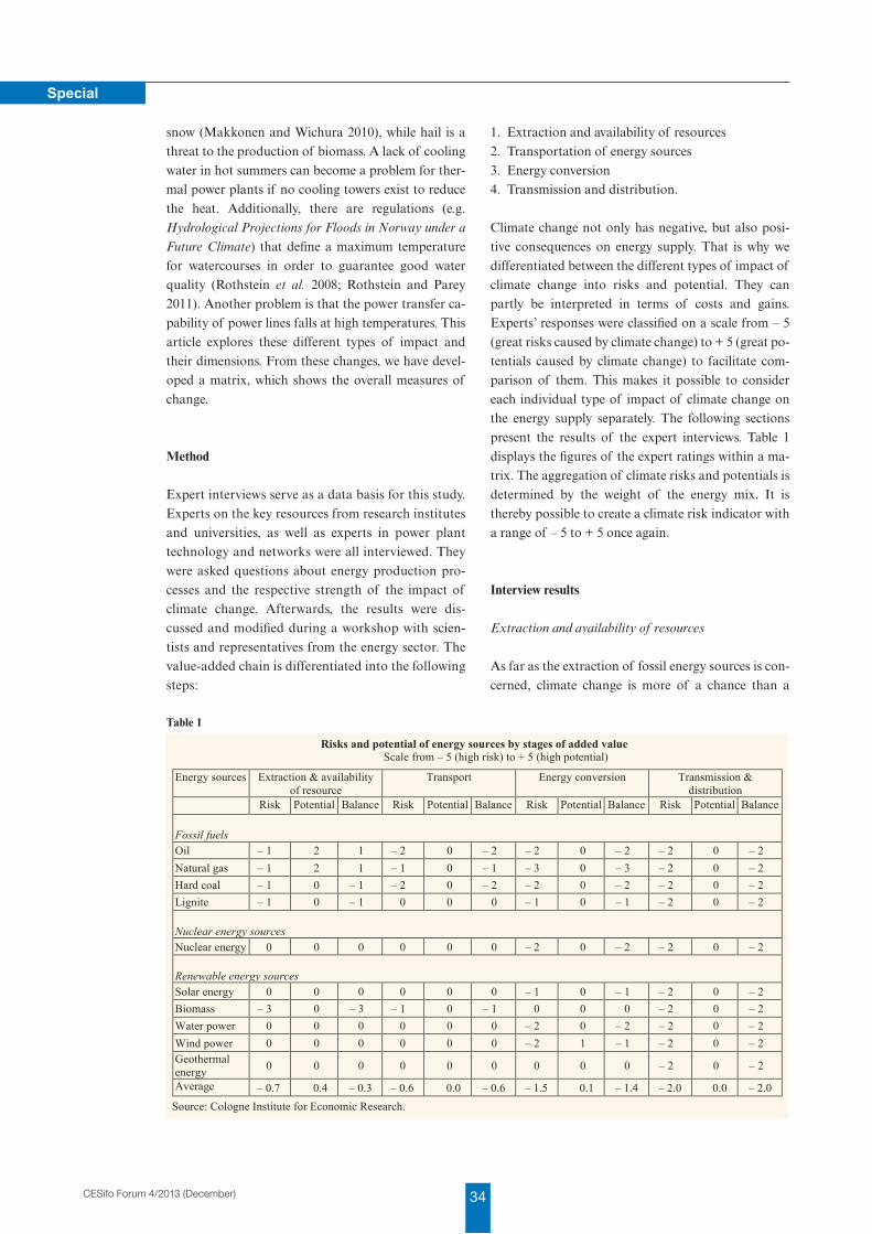
34CESifo Forum 4/2013 (December)

Special

snow (Makkonen and Wichura 2010), while hail is a threat to the production of biomass. A lack of cooling water in hot summers can become a problem for ther­mal power plants if no cooling towers exist to reduce the heat. Additionally, there are regulations (e.g. Hydrological Projections for Floods in Norway under a

Future Climate) that define a maximum temperature for watercourses in order to guarantee good water quality (Rothstein et al. 2008; Rothstein and Parey 2011). Another problem is that the power transfer ca­pability of power lines falls at high temperatures. This article explores these different types of impact and their dimensions. From these changes, we have devel­oped a matrix, which shows the overall measures of change.

Method

Expert interviews serve as a data basis for this study. Experts on the key resources from research institutes and universities, as well as experts in power plant technology and networks were all interviewed. They were asked questions about energy production pro­cesses and the respective strength of the impact of climate change. Afterwards, the results were dis­cussed and modified during a workshop with scien­tists and representatives from the energy sector. The value­added chain is differentiated into the following steps:

1. Extraction and availability of resources2. Transportation of energy sources3. Energy conversion4. Transmission and distribution.

Climate change not only has negative, but also posi­tive consequences on energy supply. That is why we differentiated between the different types of impact of climate change into risks and potential. They can partly be interpreted in terms of costs and gains. Experts’ responses were classified on a scale from – 5 (great risks caused by climate change) to + 5 (great po­tentials caused by climate change) to facilitate com­parison of them. This makes it possible to consider each individual type of impact of climate change on the energy supply separately. The following sections present the results of the expert interviews. Table 1 displays the figures of the expert ratings within a ma­trix. The aggregation of climate risks and potentials is determined by the weight of the energy mix. It is thereby possible to create a climate risk indicator with a range of – 5 to + 5 once again.

Interview results

Extraction and availability of resources

As far as the extraction of fossil energy sources is con­cerned, climate change is more of a chance than a Table 1

Risks and potential of energy sources by stages of added value Scale from – 5 (high risk) to + 5 (high potential)

Energy sources Extraction & availability of resource

Transport Energy conversion Transmission & distribution

Risk Potential Balance Risk Potential Balance Risk Potential Balance Risk Potential Balance

Fossil fuels Oil – 1 2 1 – 2 0 – 2 – 2 0 – 2 – 2 0 – 2

Natural gas – 1 2 1 – 1 0 – 1 – 3 0 – 3 – 2 0 – 2

Hard coal – 1 0 – 1 – 2 0 – 2 – 2 0 – 2 – 2 0 – 2

Lignite – 1 0 – 1 0 0 0 – 1 0 – 1 – 2 0 – 2 Nuclear energy sources Nuclear energy 0 0 0 0 0 0 – 2 0 – 2 – 2 0 – 2 Renewable energy sources Solar energy 0 0 0 0 0 0 – 1 0 – 1 – 2 0 – 2

Biomass – 3 0 – 3 – 1 0 – 1 0 0 0 – 2 0 – 2

Water power 0 0 0 0 0 0 – 2 0 – 2 – 2 0 – 2

Wind power 0 0 0 0 0 0 – 2 1 – 1 – 2 0 – 2 Geothermal energy

0 0 0 0 0 0 0 0 0 – 2 0 – 2

Average – 0.7 0.4 – 0.3 – 0.6 0.0 – 0.6 – 1.5 0.1 – 1.4 – 2.0 0.0 – 2.0

Source: Cologne Institute for Economic Research.

Table 1

35 CESifo Forum 4/2013 (December)

Special

threat. The onshore production of oil and natural gas

is hardly affected by climate change. Several sources

that could be used offshore when the pack ice melts, on

the other hand, have been inaccessible to date.

Offshore platforms, on the other hand, will have to be

lifted when the sea level rises. All in all, the risks of cli­

mate change related to the extraction of oil and natu­

ral gas are low, according to the experts.

There is another energy source that may play a more

important role in the future: methane in a hydrate

form that lies on the sea floor. Experts do not expect

any complications with the extraction of methane hy­

drate caused by climate change. Instead, bigger depos­

its will be accessible because of the reduction of ice –

as in the case of oil and natural gas. The targeted

extraction of methane hydrate also makes it possible

to stop the release of methane hydrate deposits due to

the warming of the sea bed. Therefore, by extracting

methane hydrate, it is possible to counteract the speed

of climate change. Since the material handling sys­

tems are similar to the systems used to extract oil and

natural gas, no essential problems caused by climate

change are expected.

Generally, yields of oil, natural gas and methane hy­

drate will only decrease a little because of climate

change. The given infrastructure is sufficient to com­

pensate bottlenecks.

The extraction of hard coal will not be affected by cli­

mate change – positively or negatively. However, since

imports are very important for this sector, it is neces­

sary to think about climate change’s potential impact

on world production. For example, the global market

price for coal increased at the beginning of 2011 after

the disastrous flood in Australia that flooded several

big coal mines. The extraction of coal is not affected

negatively by climate change in Europe, but it is the

case in other regions of the world.

According to experts, there may be a stronger dust

formation when extracting lignite at an open pit mine

during periods of drought. In order not to endanger

the health of the area’s residents, the lignite has to be

moistened. Generally speaking, however, longer peri­

ods of drought are positive for the production of en­

ergy from lignite because it burns easier when it is

dry. Heavy rain that can cause landslides at open pit

mines is also expected. However, short­term restric­

tions do not lead to bottlenecks due to sufficient

stocks.

Extraction of uranium for the use of nuclear energy

also takes place in open pit mines. Experts classify the

impact of climate change on the extraction of urani­

um and its possible bottlenecks as very low. Even in

the past, there have been no serious disturbances in

the production of the resources.

Biomass is another energy source. The larger part is

extracted form plants like corn, the smaller part from

waste products such as liquid manure and straw. In

view of competition from food cultivation and other

uses, the vegetable part is very likely to decrease in the

future. There may be bottlenecks in the production of

biomass, but they are more likely to be due to fluctua­

tion in prices in the global markets than to the conse­

quences of climate change. For this reason, smaller

power plants had to be shut down for a short time in

the past. The use of these resources is affected by cli­

mate change as reflected in changing precipitation pat­

terns and extreme weather events. But if these resourc­

es are stored in the right way, it is possible to prepare

for production losses.

Transportation of energy sources

Climate change can heavily impact the transportation

of energy sources when they are shipped by sea. Such

energy sources include oil, natural gas and methane

hydrate, and also (because of high imports) hard coal

and biomass. Costs are likely to increase because of

the interruption to business caused by the growing

number of storms and their increasing intensity. The

same is applicable to transport on rivers: in periods of

drought their navigability is limited due to low water

levels. The impact of climate change on transporta­

tion is negative, but does not carry too much weight.

Energy conversion

Taking a closer look at the influences of climate

change on energy production, it is important to realize

that it is not the resources used that are relevant for

the study, but the type of power plant. According to

the experts, climate change has the biggest impact on

steam power plants, which are used to generate power

from oil, natural gas, methane hydrate, hard coal and

nuclear energy. Sinking river water and groundwater

levels, as well as the rising temperatures of water­

courses, restrict the availability of cooling water dur­

ing heat waves. During these times power plants often

have to reduce their output or shut down in order to

protect the environment. That is why in the future

36CESifo Forum 4/2013 (December)

Special

stronger seasonal variation in the energy production

from affected power plants is expected. The risks still

remain in a medium range, because most of the time

only certain power plants are affected by these ex­

treme conditions. That is why there is no threat to the

power supply as a whole. Moreover, most of the newer

power plants do have cooling towers, which makes

them less vulnerable to climate change anyway.

The problem with the cooling water rarely applies to

lignite fuelled power stations, because most of them

are not cooled by water from a river anyway. Instead,

they use drained water from the open pit mine for

cooling. Should outdoor temperatures be high, effi­

ciency might be reduced. The loss of efficiency is not

very high, but still economically noticeable.

Increased outdoor temperatures play a role when it

comes to power generation from natural gas. The

higher the outdoor temperature, the lower the possible

efficiency of common power plants using cycle gas

turbines. That is why the power generation by gas

power plants is more influenced by climate change

than other types of power plants. Yet one advantage

of gas power plants is that it can bridge short­term

bottlenecks in the energy supply. But energy produc­

tion from fossil fuels is not the only form of energy

production to be affected by climate change: the latter

will also have an impact on renewable energies.

Solar energy is the renewable energy with the biggest

variations in yields. Solar thermal plants are highly

dependent on the sunshine, while photovoltaic sys­

tems can still supply energy when the sky is cloudy.

Due to climate change, the output of these plants in

Europe is expected to be low in the winter months and

high during the summer months. It is possible for the

use of solar energy to react to shifts in demand caused

by climate change: less heat demand in the winter and

more demand for cooling in the summer. Moreover,

there are fluctuations of 15 percent in the use of solar

energy due to fairly unstable weather conditions.

However, long term fluctuations of the same scale

caused by astronomical effects, like changes in the

sun, are of prime importance because there are no

other plants that can compensate for them. An impor­

tant factor in the yields from solar energy is global ra­

diation. This includes direct solar radiation, as well as

radiation components like scattering, which strike the

earth and are caused by clouds. Despite local differ­

ences, global radiation in general will not change be­

cause of climate change. Variations in temperature are

not very likely to have major implications for plants

either. Technically, the potential of solar energy is

well­known and will not be considerably altered by cli­

mate change. Plants nevertheless remain slightly vul­

nerable due to extreme weather events like storms and

hail.

Wind power stations are directly affected by climate

change. To date some plants have had to be switched

off in storms so as not to endanger their functionality.

These problems only occur for two or three hours a

year, which is economically irrelevant. Nowadays en­

gineers are working on techniques that make it possi­

ble to let the systems run on a lower capacity during a

storm. The impact of climate change on the energy

supply from wind power stations is generally limited.

Biofuel plants are also only slightly affected by higher

outdoor temperatures. The same types of bio fuel

plants are operated in different climate zones. Bio gas

plants are more sensitive to storms than others, but

even this susceptibility is low and can be neglected.

There are only problems with cooling water in very

complex systems, because others do not need much of

it. That is the reason why the risks cannot be com­

pared to the cooling water requirements of other

steam power plants.

In the case of low water levels, river power plants are

estimated to render only roughly half of their usual

service. However, since annual fluctuations are com­

mon, changing water levels are already taken into ac­

count and can therefore be compensated for through­

out the year. Moreover, there is always a basic amount

of water via the supply of cleaned water from the sew­

age plant. There are also potential ways of bridging

bottlenecks, especially through pumped­storage pow­

er plants. The drawbacks in this case are that pumped­

storage power plants mean high initial investments

and storage power plants produce less electricity dur­

ing heat waves than usual. In general, however, the im­

pact of climate change on the energy supply from wa­

ter power is low.

The use of geothermal energy as an energy resource is

quite climate robust. In our latitudes, we do not expect

any noticeable impact on power plants due to climate

change. There may be fluctuations in the energy pro­

duction from geothermal energy in certain regions

where less precipitation is expected. In Kenya, for ex­

ample, deep droughts may cause problems in energy

production.

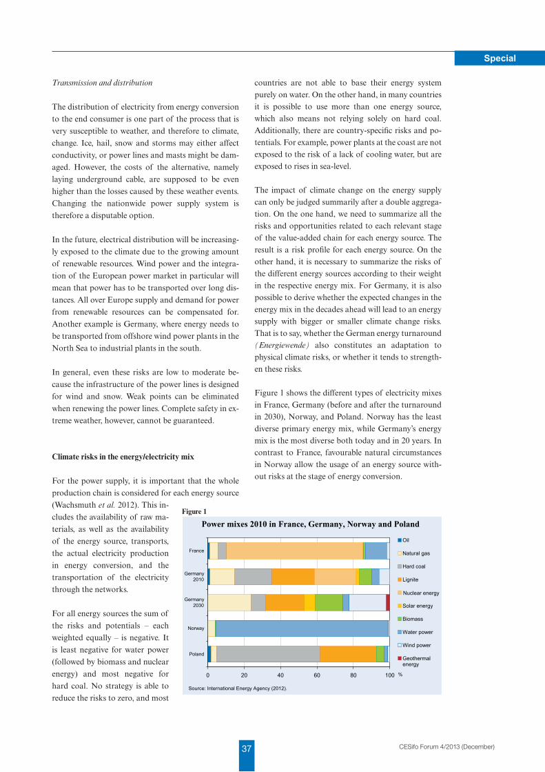
37 CESifo Forum 4/2013 (December)

Special

Transmission and distribution

The distribution of electricity from energy conversion

to the end consumer is one part of the process that is

very susceptible to weather, and therefore to climate,

change. Ice, hail, snow and storms may either affect

conductivity, or power lines and masts might be dam­

aged. However, the costs of the alternative, namely

laying underground cable, are supposed to be even

higher than the losses caused by these weather events.

Changing the nationwide power supply system is

therefore a disputable option.

In the future, electrical distribution will be increasing­

ly exposed to the climate due to the growing amount

of renewable resources. Wind power and the integra­

tion of the European power market in particular will

mean that power has to be transported over long dis­

tances. All over Europe supply and demand for power

from renewable resources can be compensated for.

Another example is Germany, where energy needs to

be transported from offshore wind power plants in the

North Sea to industrial plants in the south.

In general, even these risks are low to moderate be­

cause the infrastructure of the power lines is designed

for wind and snow. Weak points can be eliminated

when renewing the power lines. Complete safety in ex­

treme weather, however, cannot be guaranteed.

Climate risks in the energy/electricity mix

For the power supply, it is important that the whole

production chain is considered for each energy source

(Wachsmuth et al. 2012). This in­

cludes the availability of raw ma­

terials, as well as the availability

of the energy source, transports,

the actual electricity production

in energy conversion, and the

transportation of the electricity

through the networks.

For all energy sources the sum of

the risks and potentials – each

weighted equally – is negative. It

is least negative for water power

(followed by biomass and nuclear

energy) and most negative for

hard coal. No strategy is able to

reduce the risks to zero, and most

countries are not able to base their energy system purely on water. On the other hand, in many countries it is possible to use more than one energy source, which also means not relying solely on hard coal. Additionally, there are country­specific risks and po­tentials. For example, power plants at the coast are not exposed to the risk of a lack of cooling water, but are exposed to rises in sea­level.

The impact of climate change on the energy supply can only be judged summarily after a double aggrega­tion. On the one hand, we need to summarize all the risks and opportunities related to each relevant stage of the value­added chain for each energy source. The result is a risk profile for each energy source. On the other hand, it is necessary to summarize the risks of the different energy sources according to their weight in the respective energy mix. For Germany, it is also possible to derive whether the expected changes in the energy mix in the decades ahead will lead to an energy supply with bigger or smaller climate change risks. That is to say, whether the German energy turnaround (Energiewende) also constitutes an adaptation to physical climate risks, or whether it tends to strength­en these risks.

Figure 1 shows the different types of electricity mixes in France, Germany (before and after the turnaround in 2030), Norway, and Poland. Norway has the least diverse primary energy mix, while Germany’s energy mix is the most diverse both today and in 20 years. In contrast to France, favourable natural circumstances in Norway allow the usage of an energy source with­out risks at the stage of energy conversion.

0 20 40 60 80 100

Poland

Norway

Germany2030

Germany2010

France

Oil

Natural gas

Hard coal

Lignite

Solar energy

Biomass

Water power

Wind power

Geothermalenergy

Power mixes 2010 in France, Germany, Norway and Poland

Source: International Energy Agency (2012).

%

Nuclear energy

Figure 1

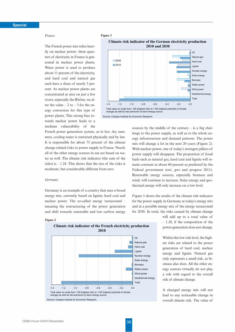
38CESifo Forum 4/2013 (December)

Special

France

The French power mix relies heav­

ily on nuclear power: three quar­

ters of electricity in France is gen­

erated in nuclear power plants.

Water power is used to produce

about 11 percent of the electricity,

and hard coal and natural gas

each have a share of nearly 5 per­

cent. As nuclear power plants are

concentrated at sites on just a few

rivers, especially the Rhône, we al­

ter the value – 2 to – 3 for the en­

ergy conversion for this type of

power plants. This strong bias to­

wards nuclear power leads to a

medium vulnerability of the

French power generation system, as in hot, dry sum­

mers, cooling water is restricted physically and by law.

It is responsible for about 75 percent of the climate

change related risks to power supply in France. Nearly

all of the other energy sources in use are based on wa­

ter as well. The climate risk indicator (the sum of the

risks) is – 1.24. This shows that the size of the risks is

moderate, but considerably different from zero.

Germany

Germany is an example of a country that uses a broad

energy mix, currently based on lignite, hard coal and

nuclear power. The so­called energy turnaround –

meaning the restructuring of the power generation

and shift towards renewable and low carbon energy

sources by the middle of the century – is a big chal­

lenge to the power supply, as well as to the whole en­

ergy infrastructure and demand patterns. The power

mix will change a lot in the next 20 years (Figure 2).

With nuclear power, one of today’s strongest pillars of

power supply will disappear. The proportion of fossil

fuels such as natural gas, hard coal and lignite will re­

main constant at about 60 percent as predicted by the

Federal government (ewi, gws and prognos 2011).

Renewable energy sources, especially biomass and

wind, will continue to increase. Solar energy and geo­

thermal energy will only increase on a low level.

Figure 3 shows the results of the climate risk indicator

for the power supply in Germany at today’s energy mix

and at a possible energy mix of the energy turnaround

for 2030. In total, the risks caused by climate change

will add up to a total value of

– 1.20, if the composition of the

power generation does not change.

Within this low risk level, the high­

est risks are related to the power

generation of hard coal, nuclear

energy and lignite. Natural gas

only represents a small risk, as bi­

omass also does. All the other en­

ergy sources virtually do not play

a role with regard to the overall

risk of climate change.

A changed energy mix will not

lead to any noticeable change in

overall climate risk. The value of

-1.4 -1.2 -1.0 -0.8 -0.6 -0.4 -0.2 0.0

Total

Geothermal energy

Wind power

Water power

Biomass

Solar energy

Nuclear energy

Lignite

Hard coal

Natural gas

Oil

Climate risk indicator of the French electricity production 2010

Source: Cologne Institute for Economic Research.

Total value on scale from -100 (highest risk) to +100 (highest potential of climate change) as well as risk premiums of each energy source.

Figure 2

-1.4 -1.2 -1.0 -0.8 -0.6 -0.4 -0.2 0.0

Total

Geothermal energy

Wind power

Water power

Biomass

Solar energy

Nuclear energy

Lignite

Hard coal

Natural gas

Oil

2030

2010

Climate risk indicator of the German electricity production 2010 and 2030

Source: Cologne Institute for Economic Research.

Total value on scale from -100 (highest risk) to +100 (highest potential of climate change) as well as risk premiums of each energy source.

Figure 3

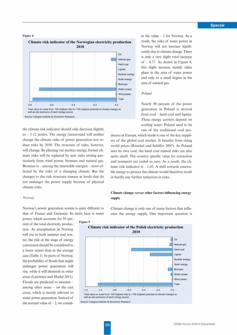
39 CESifo Forum 4/2013 (December)

Special

the climate risk indicator should only decrease slightly

to – 1.12 points. The energy turnaround will neither

change the climate risks of power generation nor re­

duce risks by 2030. The structure of risks, however,

will change. By phasing out nuclear energy, former cli­

mate risks will be replaced by new risks arising par­

ticularly from wind power, biomass and natural gas.

Biomass is – among the renewable energies – most af­

fected by the risks of a changing climate. But the

changes to the risk structure remain at levels that do

not endanger the power supply because of physical

climate risks.

Norway

Norway’s power generation system is quite different to

that of France and Germany. Its main base is water

power, which accounts for 95 per­

cent of the total electricity produc­

tion. As precipitation in Norway

will rise in both summer and win­

ter, the risk at the stage of energy

conversion should be considered to

a lesser extent than in the average

case (Table 1). In parts of Norway,

the probability of floods that might

endanger power generation will

rise, while it will diminish in other

areas (Lawrence and Hisdal 2011).

Floods are predicted to increase –

among other areas – on the east

coast, which is mostly relevant to

water power generation. Instead of

the normal value of – 2, we consid­

er the value – 1 for Norway. As a

result, the risks of water power in

Norway will not increase signifi­

cantly due to climate change. There

is only a very slight total increase

of –  0.77. As shown in Figure 4,

this slight increase mainly takes

place in the area of water power

and only to a small degree in the

area of natural gas.

Poland

Nearly 90 percent of the power

generation in Poland is derived

from coal – hard coal and lignite.

These energy carriers depend on

cooling water. Poland used to be

one of the traditional coal pro­

ducers in Europe, which made it one of the key suppli­

ers of the global coal market. It benefits from rising

world prices (Ritschel and Schiffer 2007). As Poland

uses its own coal, the hard coal related risks are also

quite small. The country specific value for extraction

and transport are coded as zero. As a result, the cli­

mate risk indicator is – 1.03. A shift towards renewa­

ble energy to protect the climate would therefore result

in hardly any further reduction in risks.

Climate change versus other factors influencing energy supply

Climate change is only one of many factors that influ­

ence the energy supply. One important question is

-0.8 -0.6 -0.4 -0.2 0.0

Total

Wind power

Water power

Biomass

Solar energy

Nuclear energy

Lignite

Hard coal

Natural gas

Oil

Climate risk indicator of the Norwegian electricity production 2010

Source: Cologne Institute for Economic Research.

Total value on scale from -100 (highest risk) to +100 (highest potential of climate change) as well as risk premiums of each energy source.

Figure 4

-1.2 -1.0 -0.8 -0.6 -0.4 -0.2 0.0

Total

Wind power

Water power

Biomass

Solar energy

Nuclear energy

Lignite

Hard coal

Natural gas

Oil

Climate risk indicator of the Polish electricity production 2010

Source: Cologne Institute for Economic Research.

Total value on scale from -100 (highest risk) to +100 (highest potential of climate change) as well as risk premiums of each energy source.

Figure 5

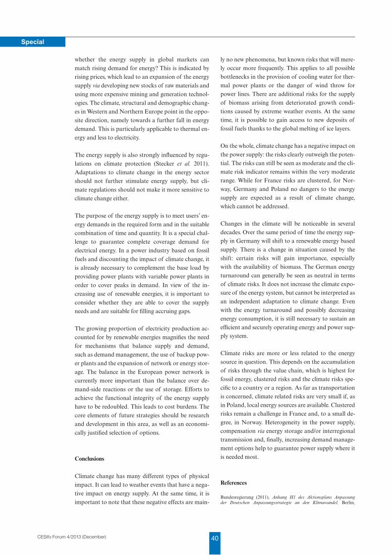
40CESifo Forum 4/2013 (December)

Special

whether the energy supply in global markets can

match rising demand for energy? This is indicated by

rising prices, which lead to an expansion of the energy

supply via developing new stocks of raw materials and

using more expensive mining and generation technol­

ogies. The climate, structural and demographic chang­

es in Western and Northern Europe point in the oppo­

site direction, namely towards a further fall in energy

demand. This is particularly applicable to thermal en­

ergy and less to electricity.

The energy supply is also strongly influenced by regu­

lations on climate protection (Stecker et al. 2011).

Adaptations to climate change in the energy sector

should not further stimulate energy supply, but cli­

mate regulations should not make it more sensitive to

climate change either.

The purpose of the energy supply is to meet users’ en­

ergy demands in the required form and in the suitable

combination of time and quantity. It is a special chal­

lenge to guarantee complete coverage demand for

electrical energy. In a power industry based on fossil

fuels and discounting the impact of climate change, it

is already necessary to complement the base load by

providing power plants with variable power plants in

order to cover peaks in demand. In view of the in­

creasing use of renewable energies, it is important to

consider whether they are able to cover the supply

needs and are suitable for filling accruing gaps.

The growing proportion of electricity production ac­

counted for by renewable energies magnifies the need

for mechanisms that balance supply and demand,

such as demand management, the use of backup pow­

er plants and the expansion of network or energy stor­

age. The balance in the European power network is

currently more important than the balance over de­

mand­side reactions or the use of storage. Efforts to

achieve the functional integrity of the energy supply

have to be redoubled. This leads to cost burdens. The

core elements of future strategies should be research

and development in this area, as well as an economi­

cally justified selection of options.

Conclusions

Climate change has many different types of physical

impact. It can lead to weather events that have a nega­

tive impact on energy supply. At the same time, it is

important to note that these negative effects are main­

ly no new phenomena, but known risks that will mere­

ly occur more frequently. This applies to all possible

bottlenecks in the provision of cooling water for ther­

mal power plants or the danger of wind throw for

power lines. There are additional risks for the supply

of biomass arising from deteriorated growth condi­

tions caused by extreme weather events. At the same

time, it is possible to gain access to new deposits of

fossil fuels thanks to the global melting of ice layers.

On the whole, climate change has a negative impact on

the power supply: the risks clearly outweigh the poten­

tial. The risks can still be seen as moderate and the cli­

mate risk indicator remains within the very moderate

range. While for France risks are clustered, for Nor­

way, Germany and Poland no dangers to the energy

supply are expected as a result of climate change,

which cannot be addressed.

Changes in the climate will be noticeable in several

decades. Over the same period of time the energy sup­

ply in Germany will shift to a renewable energy based

supply. There is a change in situation caused by the

shift: certain risks will gain importance, especially

with the availability of biomass. The German energy

turnaround can generally be seen as neutral in terms

of climate risks. It does not increase the climate expo­

sure of the energy system, but cannot be interpreted as

an independent adaptation to climate change. Even

with the energy turnaround and possibly decreasing

energy consumption, it is still necessary to sustain an

efficient and securely operating energy and power sup­

ply system.

Climate risks are more or less related to the energy

source in question. This depends on the accumulation

of risks through the value chain, which is highest for

fossil energy, clustered risks and the climate risks spe­

cific to a country or a region. As far as transportation

is concerned, climate related risks are very small if, as

in Poland, local energy sources are available. Clustered

risks remain a challenge in France and, to a small de­

gree, in Norway. Heterogeneity in the power supply,

compensation via energy storage and/or interregional

transmission and, finally, increasing demand manage­

ment options help to guarantee power supply where it

is needed most.

References

Bundesregierung (2011), Anhang H1 des Aktionsplans Anpassung der Deutschen Anpassungsstrategie an den Klimawandel, Berlin,

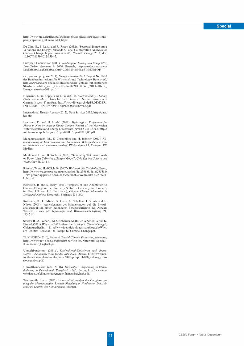
41 CESifo Forum 4/2013 (December)

Special

http://www.bmu.de/files/pdfs/allgemein/application/pdf/aktions­ plan_anpassung_klimawandel_bf.pdf.

De Cian, E., E. Lanzi and R. Roson (2012), “Seasonal Temperature Variations and Energy Demand: A Panel Cointegration Analyses for Climate Change Impact Assessment”, Climatic Change 2012, doi: 10.1007/s10584­012­0514­5.

European Commission (2011), Roadmap for Moving to a Competitive Low-Carbon Economy in 2050, Brussels, http://eur­lex.europa.eu/LexUriServ/LexUriServ.do?uri=COM:2011:0112:FIN:EN:PDF.

ewi, gws and prognos (2011), Energieszenarien 2011, Projekt Nr. 12/10 des Bundesministeriums für Wirtschaft und Technologie, Basel et al., http://www.ewi.uni­koeln.de/fileadmin/user_upload/Publikationen/ Studien/Polit ik_und_Gesellschaft/2011/EWI_2011­08­12_Energieszenarien­2011.pdf.

Heymann, E., O. Koppel and T. Puls (2011), Electromobility – Falling Costs Are a Must, Deutsche Bank Research Natural resources – Current Issues, Frankfurt, http://www.dbresearch.de/PROD/DBR_INTERNET_EN­PROD/PROD0000000000279687.pdf.

International Energy Agency (2012), Data Services 2012, http://data.iea.org

Lawrence, D. and H. Hisdal (2011), Hydrological Projections for Floods in Norway under a Future Climate, Report of the Norwegian Water Resources and Energy Directorate (NVE) 5­2011, Oslo, http://webby.nve.no/publikasjoner/report/2011/report2011_05.pdf.

Mahammadzadeh, M., E. Chrischilles and H. Biebeler (2013), Kli-maanpassung in Unternehmen und Kommunen. Betroffenheiten, Ver-letzlichkeiten und Anpassungsbedarf, IW­Analysen 83, Cologne: IW Medien.

Makkonen, L. and B. Wichura (2010), “Simulating Wet Snow Loads on Power Line Cables by a Simple Model”, Cold Regions Science and Technology 61, 73–81.

Ritschel, W. and H.­W. Schiffer (2007), Weltmarkt für Steinkohle, Essen, http://www.rwe.com/web/cms/mediablob/de/236138/data/235584/ 1/rwe­power­ag/presse­downloads/steinkohle/Weltmarkt­fuer­Stein­kohle.pdf.

Rothstein, B. and S. Parey (2011), “Impacts of and Adaptation to Climate Change in the Electricity Sector in Germany and France”, in: Ford J.D. and L.B. Ford (eds.), Climate Change Adaptation in Developed Nations, Dordrecht: Springer, 231–242.

Rothstein, B., U. Müller, S. Greis, A. Scholten, J. Schulz and E. Nilson (2008), “Auswirkungen des Klimawandels auf die Elektri­zitätsproduktion unter besonderer Berücksichtigung des Aspekts Wasser”, Forum für Hydrologie und Wasserbewirtschaftung 24, 193–214.

Stecker, R., A. Pechan, J.M. Steinhäuser, M. Rotter, G. Scholl, G. and K. Eisnack (2011), Why Are Utilities Reluctant to Adapt to Climate Change?, Oldenburg/Berlin, http://www.ioew.de/uploads/tx_ukioewdb/Why_are_Utilities_Reluctant_to_Adapt_to_Climate_Change.pdf.

TÜV NORD (2010), Network Special Climate Protection, Hannover, http://www.tuev­nord.de/cps/rde/xbcr/tng_en/Netzwerk_Spezial_Klimaschutz_Englisch.pdf.

Umweltbundesamt (2011a), Kohlendioxid-Emissionen nach Brenn-stoffen – Zeitnahprognose für das Jahr 2010, Dessau, http://www.um­weltbundesamt.de/uba­info­presse/2011/pdf/pd11­020_anhang_emis­sionsquellen.pdf.

Umweltbundesamt (eds., 2011b), Themenblatt: Anpassung an Klima-änderung in Deutschland. Energiewirtschaft, Berlin, http://www.um­weltdaten.de/klimaschutz/energie­finanzwirtschaft.pdf.

Wachsmuth, J. et al. (2012), Vulnerabilitätsanalyse der Energieversor-gung der Metropolregion Bremen-Oldenburg in Nordwesten Deutsch-lands im Kontext des Klimawandels, Bremen.

42CESifo Forum 4/2013 (December)

Special

Relative innovative CapaCity of GeRman ReGions: is east GeRmany still laGGinG Behind?

miChael BeRlemann and

veRa Jahn1

Introduction

Most economists will agree that innovation, in the

form of new products and processes for example, is a

fundamental prerequisite for economic prosperity (see

Dohse 2004). Innovation is also the key to solving

many of the world’s most pressing social challenges

such as improving the quality of the physical environ-

ment or health care. The innovative capacity of a re-

gion is rooted in its microeconomic environment and

depends, among others, on factors such as the inten-

sity of scientists and engineers in the regional work-

force and the degree of protection of intellectual

property (see Baumert, Buesa and Heijs 2010).

Since the microeconomic environment can be influ-

enced by economic policy measures, politicians have

always been interested in monitoring innovative per-

formance. A prominent example is the development in

East and West German regions. While in the early

years after German Reunification East and West

Germany converged considerably in terms of per capi-

ta GDP, this process stagnated in the late 1990s

(Berlemann and Thum 2005). A large share of the gap

in economic performance between the two parts of

Germany can be attributed to differences in total fac-

tor productivity (Berlemann and Wesselhöft 2012). In

order to be able to close the remaining gap, East

Germany needs productive and innovative enterprises.

However, various studies such as Dohse (2004) or

Eickelpasch (2009) came to the result that East

Germany is still lagging behind West Germany in inno-

1 Helmut Schmidt University Hamburg.

vative capacity due to lower R&D expenses and small-

er average firm size, for example. As a result, German

politics has engaged in various programs to increase

East German innovative capacity, see Belitz, Fleischer

and Stephan (2001); BMBF (2009 and 2010).

Little official data on innovations is available to date.

To some extent, this informational gap is closed by

survey studies (see Rammer et al. 2013). However,

firms have little incentive to publish information on

their true innovative capacity. Newly developed pro-

cesses are typically kept secret in order to take advan-

tage of new technologies as long as possible (Moser

2013). Moreover, surveys often do not allow for the

study of innovation activity on a highly disaggregated

level due to the scarcity of surveyed enterprises.

The primary aim of this paper is to deliver empirical

evidence on the relative innovative capacity of

German regions on the NUTS 3-level. Special atten-

tion is devoted to the question of whether East

German regions, in fact, still perform worse in terms

of innovation activity. In the absence of reliable data

on innovations, we follow the existing literature

(Schmookler 1962 and 1966; Sokoloff 1988; Moser

and Voena 2012) by using patents as a proxy for inno-

vative activity. As Griliches (1990, 1661) argues in his

survey, patent statistics have several advantages:

“they are available; they are by definition related to

inventiveness, and they are based on what appears to

be an objective and only slowly changing standard”.

However, using patents as indicators of innovative ac-

tivity also has several caveats. Firstly, not all innova-

tive activity is patented. Several reasons may account

for that fact. In some countries patent laws do not ex-

ist at all (Moser 2013). And even if patent laws exist,

inventors may decide not to patent their intellectual

property due to the costs incurred for example, and

opt for other available means of protecting intellec-

tual property instead such as secrecy or the absence

of any commercial interest. Due to the fact that not

all inventions are patented, patents as an absolute

measure of innovative activity will underestimate the

true level of innovative activity. Secondly, the share of

innovations that inventors choose to patent is subject

to changes over the course of time. As Moser (2013)

43 CESifo Forum 4/2013 (December)

Special

reports, secrecy was a highly effective means of pro-

tecting mid-nineteenth-century improvements in

chemicals because, at that time, competitors were un-

able to reverse engineer them. As science progressed,

the possibilities of reverse engineering grew consider-

ably, thereby increasing the incentive to patent new

chemical innovations. Whenever the share of patent-

ed innovations changes over the course of time, com-

parisons along the time-axis obviously become prob-

lematic. Thirdly, the share of innovations that in -

ventors choose to patent also varies considerably be-

tween the different sectors (Levin et al. 1987; Cohen,

Nelson and Walsh 2000; Harhoff and Hoisl 2006).

Thus, regions or countries with differing sector struc-

tures are hardly comparable on the basis of simple

patent counts.

In order to deal adequately with the three problems

mentioned, we proceed as follows. Firstly, we refrain

from trying to uncover the true level of innovative ac-

tivity in German regions. Since we have no reliable in-

formation on the share of patented innovations in all

innovations, we concentrate on constructing a meas-

ure of relative innovative capacity. Secondly, since we

have no reliable information on the development of

the share of patented innovations in all innovations

over the course of time, we refrain from including the

time dimension in our analysis. Instead, we focus on a

cross section of data. For reasons of data availability,

we choose 2008 as a sample year. Thirdly, when con-

structing our measure of innovative capacity we cor-

rect for differences in regions’ sector structure.

The remainder of the paper is organized as follows: in

the next section we outline the construction of an ad-

equate indicator of relative innovative capacity on a

regional level. We subsequently turn to a description

of the patent used and firm data. Based on these data,

we then calculate the indicator and discuss the results.

The paper ends with some conclusions.

Indicator construction

Our approach of constructing an adequate indicator

of relative innovative capacity of German NUTS 3-re-

gions is based on the idea of comparing the expected

number of patents per region with the number that ac-

tually occur. Whenever a region generates more (or

less) patents than an imaginary German region with

the same sector structure, the referring region turns

out to be overly (or insufficiently) innovative.

Formally, our indicator of relative innovative perfor-

mance of a region i, Ri, can be calculated as follows:

Let I be the number of regions, J the number of sec-

tors, Pi,j the number of patents in region i and sector j

and Ni,j the number of firms in region i and sector j.

Factual patent density in region i is then given by

(1)

with Ni being the number of firms in region i, i.e.

(2)

Whenever firms within the same sector perform simi-

larly in terms of generating innovations in all regions,

patent density is expected to vary one to one with the

structure of the regional economy. Expected patent

density is thus given by

(3)

with Dj being average patent density in sector j over all

regions i, i.e.

(4)

We then define relative innovative performance of re-

gion i as

(5)

Positive values of Ri go along with overly innovative

regions, while negative values indicate underperform-

ing regions.

In order to construct the indicator of relative innova-

tive capacity described we require two sorts of data:

patent data and data on the regional structural com-

position of the economy.

Patent data

Adequate patent data have to fulfil several require-

ments. Firstly, the data should be representative of the

innovative activity of German firms. Secondly, the

patent data must be available on the regional level, in

our case on the German NUTS 3-level. Thirdly, we

need information on how patents are distributed

among the regional economies’ sectors.

i

jiJ

j ji

jii N

NNP

D ,

1 ,

,: ∑=

⋅=

∑=

=J

jjii NN

1,

i

jiJ

jj

ei N

NDD ,

1

: ∑=

⋅=

∑

∑

=

== I

iji

I

iji

j

N

PD

1,

1,

eiii DDR −=:

44CESifo Forum 4/2013 (December)

Special

In principle, three sources of patent data could be

used to study the relative innovative performance of

German regions. These sources are related to the

three typical ways that German inventors can choose

to go when securing their intellectual property via

patenting. Firstly, when an applicant is interested in

securing the patent only for the German market,

s/he can contact the German Patent Office (Deut-

sches Patent- und Markenamt, DPMA). Secondly, if

s/he is also interested in patenting his/her invention

in other European countries, s/he can send his appli-

cation to the Euro pean Patent Office. After receiving

an application, the European Patent Office trans-

mits the application to the addressed national patent

offices. Thirdly, whenever an applicant also (or only)

seeks patenting outside Europe, s/he can take advan-

tage of the rules set out in the Patent Cooperation

Treaty (PCT), which was signed in June 1970 and en-

tered into force in January 1978. While the treaty

was initially signed by only 18 states, nowadays al-

most 150 states take part in the agreement. After an

international patent application is filed with the ap-

propriate patent office (Re ceiving Office), the appli-

cation enters an international phase. Throughout

this phase an authorized Inter national Search

Authority (ISA) conducts a systematic investigation

of patentability. In the next step the application is

forwarded to the responsible national patent offices,

which then initiate the regular patenting pro -

cedures.

In order to gain a complete picture of patent applica-

tions originating in Germany, it would be necessary

to study the records of the German Patent Office, the

European Patent Office and PCT applications. How-

ever, the three databases obviously overlap and the

filing procedures make it almost impossible to com-

bine the data from the three databases. As an alterna-

tive, one might focus the analysis on one out of the

three databases mentioned. However, doing so may

give a biased picture. Focusing on the database of the

German Patent Office may favour nationally orient-

ed firms, while using German PCT filings could over-

emphasize the importance of internationally operat-

ing enterprises. Whenever these firms are unequally

distributed among German regions, this could lead

to biased results. It seems to be reasonable to assume

that the data on German patent applications at the

European Patent Office are least problematic in this

respect. In order to study the extent to which the re-

gional distribution of patents differs in the three da-

tabases, we run simple correlation analyses.

In a first step we compare the patent applications

filed at the European Patent Office and PCT applica-

tions. Both sorts of data can be extracted from the

REGPAT Database (January 2013 edition), main-

tained by the OECD.2 Both databases allow for track-

ing of the applicants back to the regional NUTS

3-level. Moreover, both databases use the Inter-

national Patent Classi fication (IPC) to attribute the

applications to different sectors. As a result, both da-

tabases are easily comparable. Interestingly enough,

we find a very high correlation coefficient of 0.98 be-

tween the two databases on the regional level. The

correlation coefficient for applications to the IPC

groups is only slightly smaller (0.96).

In a second step we compare the patent data from the

European Patent Office with the data from the

German Patent Office. However, the German data is

only available on a federal state level (NUTS 1).3 A

comparison on this comparatively high regional level

of aggregation nevertheless leads to a high correlation

coefficient of 0.98. The comparison of sector distribu-

tion is conducted on the three-digit-IPC-level and

again delivers a comparatively high level of correla-

tion (0.89).

Overall, we conclude that focusing on the patent data-

set of the European Patent Office does not lead to bi-

ased results and we employ this data in our subse-

quent analysis.

The OECD database offers a list of applications to the

European Patent Office featuring applicants’ names

and addresses. Moreover, the REGPAT Database pro-

vides lists of the priority years4 and International

Patent Classifications (IPC) of inventions. In order to

construct a dataset including all necessary informa-

tion we merged these lists via the unique application

identification number.5 We then extracted applications

with priority year 20086 and a German applicant’s ad-

dress. Doing so left us with a list of 57,287 entries on

patent applications. However, since many of these en-

tries are related to the same inventions (e.g. because of

2 The REGPAT Database is available from the OECD on request.3 See Deutsches Patent- und Markenamt (2008).4 The priority year is the year of the first filing of a patent applica-tion to any patent office in the world. It is thus most closely connected to the date of invention (OECD 2009). We therefore follow the advice issued by the OECD (2008 and 2009) and use the priority date in or-der to reflect innovative drive.5 Observations with wrong or missing values were deleted from the dataset.6 The choice of our sample year is based on the availability of data on the sector structure on the NUTS 3-level. This sort of data, which will be described in the subsequent section, was only available for the year 2008.

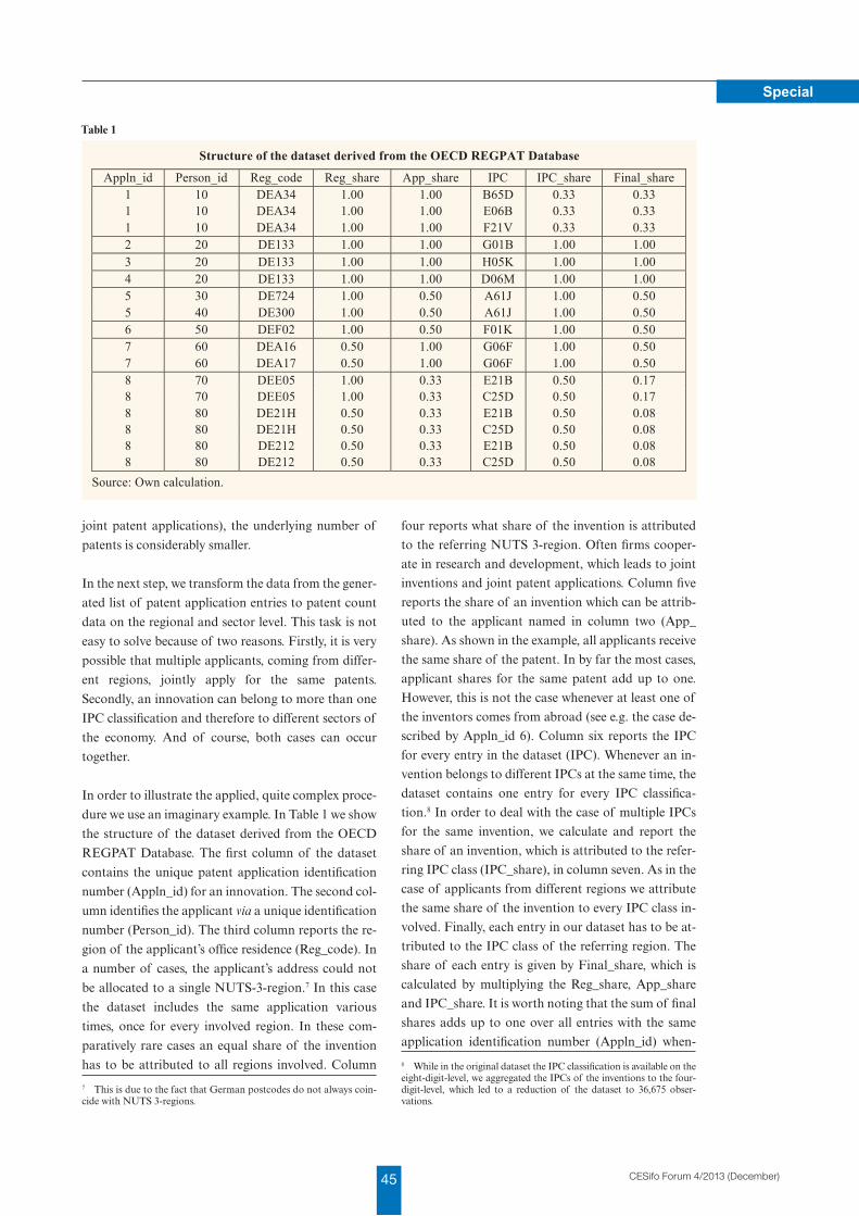
45 CESifo Forum 4/2013 (December)

Special

joint patent applications), the underlying number of

patents is considerably smaller.

In the next step, we transform the data from the gener-

ated list of patent application entries to patent count

data on the regional and sector level. This task is not

easy to solve because of two reasons. Firstly, it is very

possible that multiple applicants, coming from differ-

ent regions, jointly apply for the same patents.

Secondly, an innovation can belong to more than one

IPC classification and therefore to different sectors of

the economy. And of course, both cases can occur

together.

In order to illustrate the applied, quite complex proce-

dure we use an imaginary example. In Table 1 we show

the structure of the dataset derived from the OECD

REGPAT Database. The first column of the dataset

contains the unique patent application identification

number (Appln_id) for an innovation. The second col-

umn identifies the applicant via a unique identification

number (Person_id). The third column reports the re-

gion of the applicant’s office residence (Reg_code). In

a number of cases, the applicant’s address could not

be allocated to a single NUTS-3-region.7 In this case

the dataset includes the same application various

times, once for every involved region. In these com-

paratively rare cases an equal share of the invention

has to be attributed to all regions involved. Column

7 This is due to the fact that German postcodes do not always coin-cide with NUTS 3-regions.

four reports what share of the invention is attributed

to the referring NUTS 3-region. Often firms cooper-

ate in research and development, which leads to joint

inventions and joint patent applications. Column five

reports the share of an invention which can be attrib-

uted to the applicant named in column two (App_

share). As shown in the example, all applicants receive

the same share of the patent. In by far the most cases,

applicant shares for the same patent add up to one.

However, this is not the case whenever at least one of

the inventors comes from abroad (see e.g. the case de-

scribed by Appln_id 6). Column six reports the IPC

for every entry in the dataset (IPC). Whenever an in-

vention belongs to different IPCs at the same time, the

dataset contains one entry for every IPC classifica-

tion.8 In order to deal with the case of multiple IPCs

for the same invention, we calculate and report the

share of an invention, which is attributed to the refer-

ring IPC class (IPC_share), in column seven. As in the

case of applicants from different regions we attribute

the same share of the invention to every IPC class in-

volved. Finally, each entry in our dataset has to be at-

tributed to the IPC class of the referring region. The

share of each entry is given by Final_share, which is

calculated by multiplying the Reg_share, App_share

and IPC_share. It is worth noting that the sum of final

shares adds up to one over all entries with the same

application identification number (Appln_id) when-

8 While in the original dataset the IPC classification is available on the eight-digit-level, we aggregated the IPCs of the inventions to the four-digit-level, which led to a reduction of the dataset to 36,675 obser - vations.

Table 1

Structure of the dataset derived from the OECD REGPAT Database

Appln_id Person_id Reg_code Reg_share App_share IPC IPC_share Final_share 1 10 DEA34 1.00 1.00 B65D 0.33 0.33 1 10 DEA34 1.00 1.00 E06B 0.33 0.33 1 10 DEA34 1.00 1.00 F21V 0.33 0.33 2 20 DE133 1.00 1.00 G01B 1.00 1.00 3 20 DE133 1.00 1.00 H05K 1.00 1.00 4 20 DE133 1.00 1.00 D06M 1.00 1.00 5 30 DE724 1.00 0.50 A61J 1.00 0.50 5 40 DE300 1.00 0.50 A61J 1.00 0.50 6 50 DEF02 1.00 0.50 F01K 1.00 0.50 7 60 DEA16 0.50 1.00 G06F 1.00 0.50 7 60 DEA17 0.50 1.00 G06F 1.00 0.50 8 70 DEE05 1.00 0.33 E21B 0.50 0.17 8 70 DEE05 1.00 0.33 C25D 0.50 0.17 8 80 DE21H 0.50 0.33 E21B 0.50 0.08 8 80 DE21H 0.50 0.33 C25D 0.50 0.08 8 80 DE212 0.50 0.33 E21B 0.50 0.08 8 80 DE212 0.50 0.33 C25D 0.50 0.08

Source: Own calculation.

Table 1

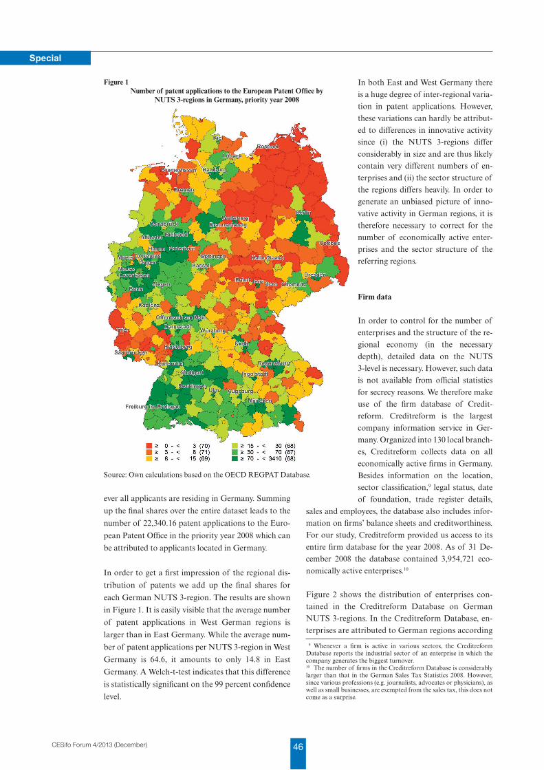
46CESifo Forum 4/2013 (December)

Special

ever all applicants are residing in Germany. Summing

up the final shares over the entire dataset leads to the

number of 22,340.16 patent applications to the Euro-

pean Patent Office in the priority year 2008 which can

be attributed to applicants located in Germany.

In order to get a first impression of the regional dis-

tribution of patents we add up the final shares for

each German NUTS 3-region. The results are shown

in Figure 1. It is easily visible that the average number

of patent applications in West German regions is

larger than in East Germany. While the average num-

ber of patent applications per NUTS 3-region in West

Ger many is 64.6, it amounts to only 14.8 in East

Germany. A Welch-t-test indicates that this difference

is statistically significant on the 99 percent confidence

level.

In both East and West Germany there is a huge degree of inter-regional varia-tion in patent applications. However, these variations can hardly be attribut-ed to differences in innovative activity since (i) the NUTS 3-regions differ considerably in size and are thus likely contain very different numbers of en-terprises and (ii) the sector structure of the regions differs heavily. In order to generate an unbiased picture of inno-vative activity in German regions, it is therefore necessary to correct for the number of economically active enter-prises and the sector structure of the referring regions.

Firm data

In order to control for the number of enterprises and the structure of the re-gional economy (in the necessary depth), detailed data on the NUTS 3-level is necessary. However, such data is not available from official statistics for secrecy reasons. We therefore make use of the firm database of Credit-reform. Creditreform is the largest company information service in Ger-many. Organized into 130 local branch-es, Creditreform collects data on all economically active firms in Germany. Besides information on the location, sector classification,9 legal status, date of foundation, trade register details,

sales and employees, the database also includes infor-mation on firms’ balance sheets and creditworthiness. For our study, Creditreform provided us access to its entire firm database for the year 2008. As of 31 De-cember 2008 the database contained 3,954,721 eco-nomically active enterprises.10

Figure 2 shows the distribution of enterprises con-tained in the Creditreform Database on German NUTS 3-regions. In the Creditreform Database, en-terprises are attributed to German regions according

9 Whenever a firm is active in various sectors, the Creditreform Database reports the industrial sector of an enterprise in which the company generates the biggest turnover.10 The number of firms in the Creditreform Database is considerably larger than that in the German Sales Tax Statistics 2008. However, since various professions (e.g. journalists, advocates or physicians), as well as small businesses, are exempted from the sales tax, this does not come as a surprise.

Figure 1Number of patent applications to the European Patent Office by

NUTS 3-regions in Germany, priority year 2008

Source: Own calculations based on the OECD REGPAT Database.

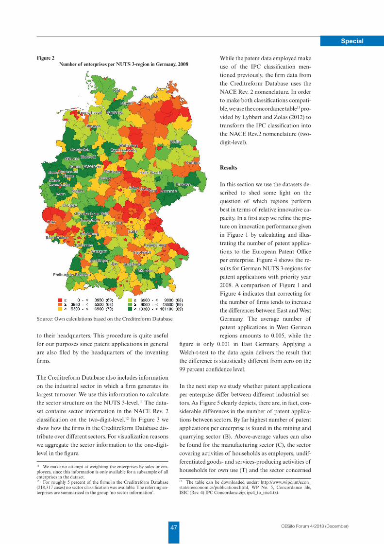
47 CESifo Forum 4/2013 (December)

Special

to their headquarters. This procedure is quite useful for our purposes since patent applications in general are also filed by the headquarters of the inventing firms.

The Creditreform Database also includes information on the industrial sector in which a firm generates its largest turnover. We use this information to calculate the sector structure on the NUTS 3-level.11 The data-set contains sector information in the NACE Rev. 2 classification on the two-digit-level.12 In Figure 3 we show how the firms in the Creditreform Database dis-tribute over different sectors. For visualization reasons we aggregate the sector information to the one-digit-level in the figure.

11 We make no attempt at weighting the enterprises by sales or em-ployees, since this information is only available for a subsample of all enterprises in the dataset.12 For roughly 5 percent of the firms in the Creditreform Database (218,317 cases) no sector classification was available. The referring en-terprises are summarized in the group ‘no sector information’.

While the patent data employed make use of the IPC classification men-tioned previously, the firm data from the Creditreform Database uses the NACE Rev. 2 nomenclature. In order to make both classifications compati-ble, we use the concordance table13 pro - vided by Lybbert and Zolas (2012) to transform the IPC classification into the NACE Rev.2 nomenclature (two- digit-level).

Results

In this section we use the datasets de-scribed to shed some light on the question of which regions perform best in terms of relative innovative ca-pacity. In a first step we refine the pic-ture on innovation performance given in Figure 1 by calculating and illus-trating the number of patent applica-tions to the European Patent Office per enterprise. Figure 4 shows the re-sults for German NUTS 3-regions for patent applications with priority year 2008. A comparison of Figure 1 and Figure 4 indicates that correcting for the number of firms tends to increase the differences between East and West Germany. The average number of patent applications in West German regions amounts to 0.005, while the

figure is only 0.001 in East Germany. Applying a Welch-t-test to the data again delivers the result that the difference is statistically different from zero on the 99 percent confidence level.

In the next step we study whether patent applications per enterprise differ between different industrial sec-tors. As Figure 5 clearly depicts, there are, in fact, con-siderable differences in the number of patent applica-tions between sectors. By far highest number of patent applications per enterprise is found in the mining and quarrying sector (B). Above-average values can also be found for the manufacturing sector (C), the sector covering activities of households as employers, undif-ferentiated goods- and services-producing activities of households for own use (T) and the sector concerned

13 The table can be downloaded under: http://www.wipo.int/econ_stat/en/economics/publications.html, WP No. 5, Concordance file, ISIC (Rev. 4) IPC Concordanc.zip, ipc4_to_isic4.txt.

Figure 2Number of enterprises per NUTS 3-region in Germany, 2008

Source: Own calculations based on the Creditreform Database.

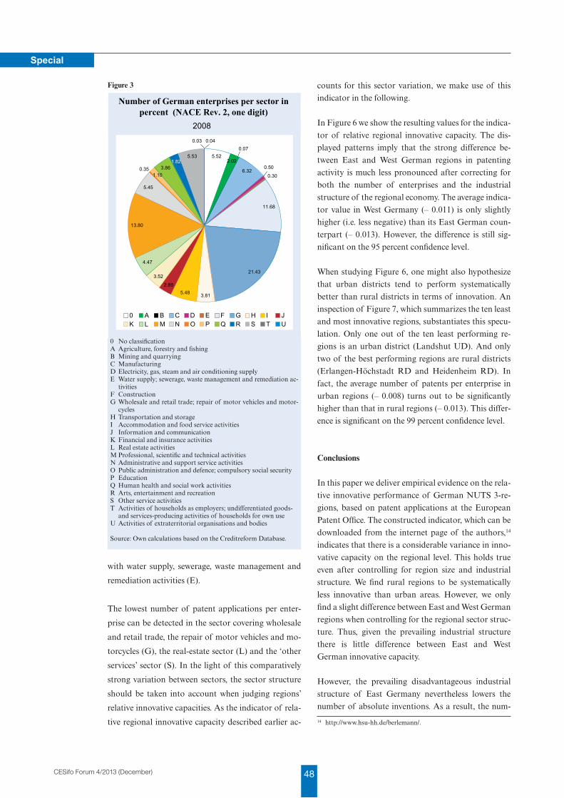
48CESifo Forum 4/2013 (December)

Special

with water supply, sewerage, waste management and

remediation activities (E).

The lowest number of patent applications per enter-

prise can be detected in the sector covering wholesale

and retail trade, the repair of motor vehicles and mo-

torcycles (G), the real-estate sector (L) and the ‘other

services’ sector (S). In the light of this comparatively

strong variation between sectors, the sector structure

should be taken into account when judging regions’

relative innovative capacities. As the indicator of rela-

tive regional innovative capacity described earlier ac-

counts for this sector variation, we make use of this

indicator in the following.

In Figure 6 we show the resulting values for the indica-

tor of relative regional innovative capacity. The dis-

played patterns imply that the strong difference be-

tween East and West German regions in patenting

activity is much less pronounced after correcting for

both the number of enterprises and the industrial

structure of the regional economy. The average indica-

tor value in West Germany (– 0.011) is only slightly

higher (i.e. less negative) than its East German coun-

terpart (– 0.013). However, the difference is still sig-

nificant on the 95 percent confidence level.

When studying Figure 6, one might also hypothesize

that urban districts tend to perform systematically

better than rural districts in terms of innovation. An

inspection of Figure 7, which summarizes the ten least

and most innovative regions, substantiates this specu-

lation. Only one out of the ten least performing re-

gions is an urban district (Landshut UD). And only

two of the best performing regions are rural districts

(Erlangen-Höchstadt RD and Heidenheim RD). In

fact, the average number of patents per enterprise in

urban regions (– 0.008) turns out to be significantly

higher than that in rural regions (– 0.013). This differ-

ence is significant on the 99 percent confidence level.

Conclusions

In this paper we deliver empirical evidence on the rela-

tive innovative performance of German NUTS 3-re-

gions, based on patent applications at the European

Patent Office. The constructed indicator, which can be

downloaded from the internet page of the authors,14

indicates that there is a considerable variance in inno-

vative capacity on the regional level. This holds true

even after controlling for region size and industrial

structure. We find rural regions to be systematically

less innovative than urban areas. However, we only

find a slight difference between East and West German

regions when controlling for the regional sector struc-

ture. Thus, given the prevailing industrial structure

there is little difference between East and West

German innovative capacity.

However, the prevailing disadvantageous industrial

structure of East Germany nevertheless lowers the

number of absolute inventions. As a result, the num-

14 http://www.hsu-hh.de/berlemann/.

5.522.02

6.32

11.68

21.43

3.815.482.89

3.52

4.47

13.80

5.45

1.103.86

5.53

0.03 0.04

1.820.35

0.07

0.30

0.50

0 A B C D E F G H I JK L M N O P Q R S T U

Number of German enterprises per sector in percent (NACE Rev. 2, one digit)

2008

Figure 3

0 No classificationA Agriculture, forestry and fishingB Mining and quarryingC ManufacturingD Electricity, gas, steam and air conditioning supplyE Water supply; sewerage, waste management and remediation ac - tivitiesF ConstructionG Wholesale and retail trade; repair of motor vehicles and motor - cyclesH Transportation and storageI Accommodation and food service activitiesJ Information and communicationK Financial and insurance activitiesL Real estate activitiesM Professional, scientific and technical activitiesN Administrative and support service activitiesO Public administration and defence; compulsory social securityP EducationQ Human health and social work activitiesR Arts, entertainment and recreationS Other service activitiesT Activities of households as employers; undifferentiated goods- and services-producing activities of households for own useU Activities of extraterritorial organisations and bodies

Source: Own calculations based on the Creditreform Database.

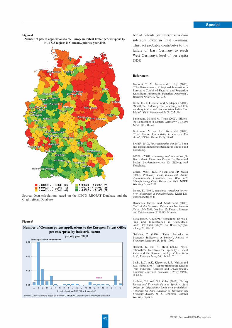
49 CESifo Forum 4/2013 (December)

Special

ber of patents per enterprise is con-

siderably lower in East Germany.

This fact probably contributes to the

failure of East Germany to reach

West Germany’s level of per capita

GDP.

References

Baumert, T., M. Buesa and J. Heijs (2010), “The Determinants of Regional Innovation in Europe: A Combined Factorial and Regression Knowledge Production Function Approach”, Research Policy 39, 722–735.

Belitz, H., F. Fleischer and A. Stephan (2001), “Staatliche Förderung von Forschung und Ent-wicklung in der ostdeutschen Wirtschaft – Eine Bilanz”, DIW Wochenbericht 68, 537–544.

Berlemann, M. and M. Thum (2005), “Bloom-ing Landscapes in Eastern Germany?”, CESifo Forum 6(4), 16–22.

Berlemann, M. and J.-E. Wesselhöft (2012), “Total Factor Productivity in German Re-gions”, CESifo Forum 13(2), 58–65.

BMBF (2010), Innovationsatlas Ost 2010, Bonn and Berlin: Bundesministerium für Bildung und Forschung.

BMBF (2009), Forschung und Innovation für Deutschland: Bilanz und Perspektive, Bonn and Berlin: Bundesministerium für Bildung und Forschung.

Cohen, W.M., R.R. Nelson and J.P. Walsh (2000), Protecting Their Intellectual Assets: Appropriability Conditions and Why U.S. Manufacturing Firms Patent (or Not), NBER Working Paper 7552.

Dohse, D. (2004), Regionale Verteilung innova-tiver Aktivitäten in Ostdeutschland, Kieler Dis-kussionsbeiträge 411.

Deutsches Patent- und Markenamt (2008), Statistik des Deutschen Patent- und Markenamts für das Jahr 2008, Das Blatt für Patent-, Muster- und Zeichenwesen (BIPMZ), Munich.

Eickelpasch, A. (2009), “Forschung, Entwick-lung und Innovationen in Ostdeutsch - land”, Vierteljahreshefte zur Wirtschaftsfor-schung 78, 78–109.

Griliches, Z. (1990), “Patent Statistics as Economic Indicators: A Survey”, Journal of Economic Literature 28, 1661–1707.

Harhoff, D. and K. Hoisl (2006), “Insti-tutionalized Incentives for Ingenuity – Patent Value and the German Employees’ Inventions Act”, Research Policy 36, 1143–1162.

Levin, R.C., A.K. Klevorick, R.R. Nelson and S.G. Winter (1987), “Appropriating the Returns from Industrial Research and Development”, Brookings Papers on Economic Activity 3/1987, 783–832.

Lybbert, T.J. and N.J. Zolas (2012), Getting Patents and Economic Data to Speak to Each Other: An “Algorithmic Links with Probabilies” Approach for Joint Analyses of Patenting and Economic Activity, WIPO Economic Research Working Paper 5.

Figure 4Number of patent applications to the European Patent Office per enterprise by

NUTS 3-regions in Germany, priority year 2008

Source: Own calculations based on the OECD REGPAT Database and the Creditreform Database.

0.00

0.05

0.10

0.15

A B C D E F G H I J K L M N O P Q R S T U

Number of German patent applications to the Europen Patent Office per enterprise by industrial sector

Source: Own calculations based on the OECD REGPAT Database and Creditreform Database.

Patent applications per enterprisepriority year 2008

mean

Industrial sectors (NACE Rev. 2, one digit)

Figure 5

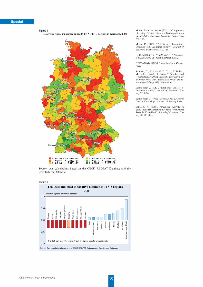
50CESifo Forum 4/2013 (December)

Special

Moser, P. and A. Voena (2012), “Compulsory Licensing: Evidence from the Trading-with-the-Enemy-Act”, American Economic Review  102, 396–427.

Moser, P. (2013), “Patents and Innovation: Evidence from Economic History”, Journal of Economic Perspectives 27, 23–44.

OECD (2008), The OECD REGPAT Database: A Presentation, STI Working Paper 2008/2.

OECD (2009), OECD Patent Statistics Manual, Paris.

Rammer, C., B. Aschoff, D. Crass, T. Doherr, M. Hud, C. Köhler, B. Peters, T. Schubert and F. Schiebacher (2013), Innovationsverhalten der deutschen Wirtschaft: Indikatorenbericht zur In-no vationserhebung 2012, Mannheim.

Schmookler, J. (1962), “Economic Sources of Inventive Activity”, Journal of Economic His-tory 22, 1–20.

Schmookler, J. (1966), Invention and Economic Growth, Cambridge: Harvard University Press.

Sokoloff, K. (1988), “Incentive Activity in Early Industrial America: Evidence from Patent Records, 1790–1846”, Journal of Economic His-tory 48, 815–850.

Figure 6Relative regional innovative capacity by NUTS-3-regions in Germany, 2008

Source: own calculations based on the OECD REGPAT Database and the Creditreform Database.

-0.10

-0.05

0.00

0.05

0.10

Fre

isin

g

Erd

ing

Ost

hols

tein

Cux

have

n

Din

golfi

ng-L

anda

u

Lan

dshu

t

Gro

ß-G

erau

Dith

mar

sche

n

Mär

kisc

h-O

derla

nd

Lan

dshu

t

Jen

a

Erla

ngen

-Höc

hsta

dt

Hei

delb

erg

Wol

fsbu

rg

Dar

mst

adt

Hei

denh

eim

Mun

ich

Stu

ttgar

t

Lev

erku

sen

Lud

wig

shaf

en a

. Rhe

in

Ten least and most innovative German NUTS-3 regions

Source: Own calculations based on the OECD REGPAT Database and Creditreform Database.

Relative regional innovative capacity2008

The dark bars stand for rural districtsl, the lighter ones for urban districts.

Figure 7

51 CESifo Forum 4/2013 (December)

Special

Ifo World EconomIc SurvEy and thE BuSInESS cyclE In SElEctEd countrIES

EvgEnIa KudymoWa, Johanna PlEnK

and KlauS WohlraBE1

The Ifo World Economic Survey is an international

economic survey that has been conducted by the Ifo

Institute on a quarterly basis since 1981. Economic ex-

perts from a large number of countries are asked to

assess the current economic situation, the economic

outlook and other economic data in their respective

field. In recent years, WES results have attracted a

growing amount of attention from national and inter-

national media. The following study examines the va-

lidity of the WES survey results in relation to the busi-

ness cycle in selected countries. To this end the Ifo

economic climate for a country is compared with the

corresponding annual growth rates of real gross do-

mestic product.

Concept of the World Economic Survey

The main focus of the Ifo World Economic Survey

(WES) is to provide an accurate picture of the current

economic situation, as well as economic trends for im-

portant advanced economies, emerging markets and

developing countries by polling over 1,000 economic

experts on a quarterly basis. Unlike the official statis-

tics, which are largely based on quantitative informa-

tion, WES focuses on qualitative information by ask-

ing economists to assess main economic indicators for

the present and for the near-term future. This allows

for a rapid, up-to-date assessment of the economic sit-

uation prevailing around the world, and particularly

in developing and transition economies, which often

have deficits in their official statistics. The uniform

questionnaire, methodology and data processing

guarantee international comparability and the aggre-

1 Ifo Institute.

gation of country results according to various country

groups, as well as comparability over time. In addi-

tion, the survey is not limited to certain product

groups, industries or companies, but concentrates on

economies as a whole.

The selection of the experts involved in this survey fo-

cuses not on a high number of respondents in the re-

spective countries, but rather on the expertise in eco-

nomic questions of the economic experts surveyed.

That means the question of representativeness thus

does not depend on the number of experts in the sur-

veyed countries, but on an accurate portrayal of the

national economies examined. Although all respond-

ents are highly qualified, the panel members are very

heterogeneous with respect to their professional occu-

pation, which covers multinational companies and in-

stitutions, economic research institutes, national and

international chambers of industry and trade or foun-

dations. Participation in the survey is absolutely vol-

untary. The questionnaire consists of eight standard

questions and regularly recurring additional ques-

tions. For the study, the relevant questions of the sur-

vey are those that concern the assessments of the pre-

sent economic situation and economic expectations

for the next six months, whose arithmetic mean forms

the economic climate indicator for each country.

About 1,200 respondents currently participate in the

survey, which covers around 120 countries. This re-

sults in a breakdown of ten questionnaires on average

for each country and quarter. In fact, the number of

respondents differs strongly across the economies sur-

veyed and ranges from 4 up to 40. Generally, the more

a country is considered as economically important (in

accordance with that country’s trade share in total

world trade), the more survey participants for the re-

spective economy are chosen.

There are three possible response categories for the as-

sessment of the present economic situation and the

economic expectations for the next six months: ‘good/

better’ for positive replies on the current situation or

expected improvement, ‘satisfactory/about the same’

for neutral replies or an unchanged expected situation

and ‘bad/worse’ for negative replies or an expected de-

terioration in the next six months. The individual re-

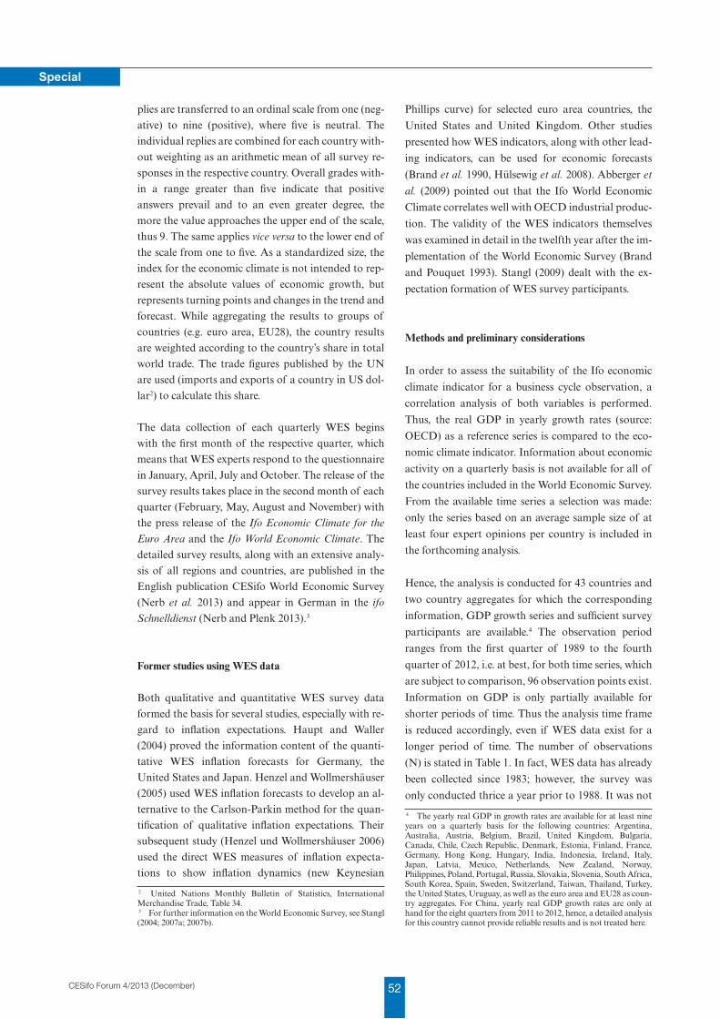
52CESifo Forum 4/2013 (December)

Special

plies are transferred to an ordinal scale from one (neg-

ative) to nine (positive), where five is neutral. The

individual replies are combined for each country with-

out weighting as an arithmetic mean of all survey re-

sponses in the respective country. Overall grades with-

in a range greater than five indicate that positive

answers prevail and to an even greater degree, the

more the value approaches the upper end of the scale,

thus 9. The same applies vice versa to the lower end of

the scale from one to five. As a standardized size, the

index for the economic climate is not intended to rep-

resent the absolute values of economic growth, but

represents turning points and changes in the trend and

forecast. While aggregating the results to groups of

countries (e.g. euro area, EU28), the country results

are weighted according to the country’s share in total

world trade. The trade figures published by the UN

are used (imports and exports of a country in US dol-

lar2) to calculate this share.

The data collection of each quarterly WES begins

with the first month of the respective quarter, which

means that WES experts respond to the questionnaire

in January, April, July and October. The release of the

survey results takes place in the second month of each

quarter (February, May, August and November) with

the press release of the Ifo Economic Climate for the

Euro Area and the Ifo World Economic Climate. The

detailed survey results, along with an extensive analy-

sis of all regions and countries, are published in the

English publication CESifo World Economic Survey

(Nerb et al. 2013) and appear in German in the ifo

Schnelldienst (Nerb and Plenk 2013).3

Former studies using WES data

Both qualitative and quantitative WES survey data

formed the basis for several studies, especially with re-

gard to inflation expectations. Haupt and Waller

(2004) proved the information content of the quanti-

tative WES inflation forecasts for Germany, the

United States and Japan. Henzel and Wollmershäuser

(2005) used WES inflation forecasts to develop an al-

ternative to the Carlson-Parkin method for the quan-

tification of qualitative inflation expectations. Their

subsequent study (Henzel und Wollmershäuser 2006)

used the direct WES measures of inflation expecta-

tions to show inflation dynamics (new Keynesian

2 United Nations Monthly Bulletin of Statistics, International Merchandise Trade, Table 34. 3 For further information on the World Economic Survey, see Stangl (2004; 2007a; 2007b).

Phillips curve) for selected euro area countries, the

United States and United Kingdom. Other studies

presented how WES indicators, along with other lead-

ing indicators, can be used for economic forecasts

(Brand et al. 1990, Hülsewig et al. 2008). Abberger et

al. (2009) pointed out that the Ifo World Economic

Climate correlates well with OECD industrial produc-

tion. The validity of the WES indicators themselves

was examined in detail in the twelfth year after the im-

plementation of the World Economic Survey (Brand

and Pouquet 1993). Stangl (2009) dealt with the ex-

pectation formation of WES survey participants.

Methods and preliminary considerations

In order to assess the suitability of the Ifo economic

climate indicator for a business cycle observation, a

correlation analysis of both variables is performed.

Thus, the real GDP in yearly growth rates (source:

OECD) as a reference series is compared to the eco-

nomic climate indicator. Information about economic

activity on a quarterly basis is not available for all of

the countries included in the World Economic Survey.

From the available time series a selection was made:

only the series based on an average sample size of at

least four expert opinions per country is included in

the forthcoming analysis.

Hence, the analysis is conducted for 43 countries and

two country aggregates for which the corresponding

information, GDP growth series and sufficient survey

participants are available.4 The observation period

ranges from the first quarter of 1989 to the fourth

quarter of 2012, i.e. at best, for both time series, which

are subject to comparison, 96 observation points exist.

Information on GDP is only partially available for

shorter periods of time. Thus the analysis time frame

is reduced accordingly, even if WES data exist for a

longer period of time. The number of observations

(N) is stated in Table 1. In fact, WES data has already

been collected since 1983; however, the survey was

only conducted thrice a year prior to 1988. It was not

4 The yearly real GDP in growth rates are available for at least nine years on a quarterly basis for the following countries: Argentina, Australia, Austria, Belgium, Brazil, United Kingdom, Bulgaria, Canada, Chile, Czech Republic, Denmark, Estonia, Finland, France, Germany, Hong Kong, Hungary, India, Indonesia, Ireland, Italy, Japan, Latvia, Mexico, Netherlands, New Zealand, Norway, Philippines, Poland, Portugal, Russia, Slovakia, Slovenia, South Africa, South Korea, Spain, Sweden, Switzerland, Taiwan, Thailand, Turkey, the United States, Uruguay, as well as the euro area and EU28 as coun-try aggregates. For China, yearly real GDP growth rates are only at hand for the eight quarters from 2011 to 2012, hence, a detailed analysis for this country cannot provide reliable results and is not treated here.

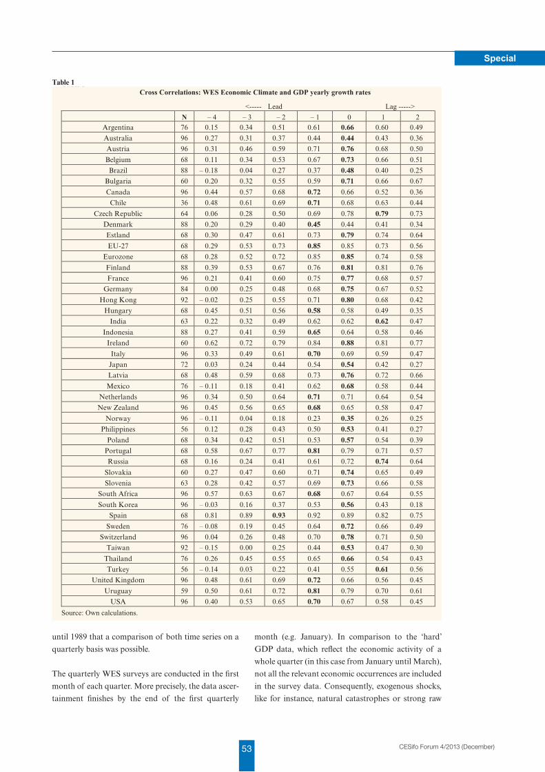
53 CESifo Forum 4/2013 (December)

Special

until 1989 that a comparison of both time series on a

quarterly basis was possible.

The quarterly WES surveys are conducted in the first

month of each quarter. More precisely, the data ascer-

tainment finishes by the end of the first quarterly

month (e.g. January). In comparison to the ‘hard’

GDP data, which reflect the economic activity of a

whole quarter (in this case from January until March),

not all the relevant economic occurrences are included

in the survey data. Consequently, exogenous shocks,

like for instance, natural catastrophes or strong raw

Table 1 Cross Correlations: WES Economic Climate and GDP yearly growth rates

<----- Lead

Lag -----> N – 4 – 3 – 2 – 1 0 1 2

Argentina 76 0.15 0.34 0.51 0.61 0.66 0.60 0.49

Australia 96 0.27 0.31 0.37 0.44 0.44 0.43 0.36

Austria 96 0.31 0.46 0.59 0.71 0.76 0.68 0.50

Belgium 68 0.11 0.34 0.53 0.67 0.73 0.66 0.51

Brazil 88 – 0.18 0.04 0.27 0.37 0.48 0.40 0.25

Bulgaria 60 0.20 0.32 0.55 0.59 0.71 0.66 0.67

Canada 96 0.44 0.57 0.68 0.72 0.66 0.52 0.36

Chile 36 0.48 0.61 0.69 0.71 0.68 0.63 0.44

Czech Republic 64 0.06 0.28 0.50 0.69 0.78 0.79 0.73

Denmark 88 0.20 0.29 0.40 0.45 0.44 0.41 0.34

Estland 68 0.30 0.47 0.61 0.73 0.79 0.74 0.64

EU-27 68 0.29 0.53 0.73 0.85 0.85 0.73 0.56

Eurozone 68 0.28 0.52 0.72 0.85 0.85 0.74 0.58

Finland 88 0.39 0.53 0.67 0.76 0.81 0.81 0.76

France 96 0.21 0.41 0.60 0.75 0.77 0.68 0.57

Germany 84 0.00 0.25 0.48 0.68 0.75 0.67 0.52

Hong Kong 92 – 0.02 0.25 0.55 0.71 0.80 0.68 0.42

Hungary 68 0.45 0.51 0.56 0.58 0.58 0.49 0.35

India 63 0.22 0.32 0.49 0.62 0.62 0.62 0.47

Indonesia 88 0.27 0.41 0.59 0.65 0.64 0.58 0.46

Ireland 60 0.62 0.72 0.79 0.84 0.88 0.81 0.77

Italy 96 0.33 0.49 0.61 0.70 0.69 0.59 0.47

Japan 72 0.03 0.24 0.44 0.54 0.54 0.42 0.27

Latvia 68 0.48 0.59 0.68 0.73 0.76 0.72 0.66

Mexico 76 – 0.11 0.18 0.41 0.62 0.68 0.58 0.44

Netherlands 96 0.34 0.50 0.64 0.71 0.71 0.64 0.54

New Zealand 96 0.45 0.56 0.65 0.68 0.65 0.58 0.47

Norway 96 – 0.11 0.04 0.18 0.23 0.35 0.26 0.25

Philippines 56 0.12 0.28 0.43 0.50 0.53 0.41 0.27

Poland 68 0.34 0.42 0.51 0.53 0.57 0.54 0.39

Portugal 68 0.58 0.67 0.77 0.81 0.79 0.71 0.57

Russia 68 0.16 0.24 0.41 0.61 0.72 0.74 0.64

Slovakia 60 0.27 0.47 0.60 0.71 0.74 0.65 0.49

Slovenia 63 0.28 0.42 0.57 0.69 0.73 0.66 0.58

South Africa 96 0.57 0.63 0.67 0.68 0.67 0.64 0.55

South Korea 96 – 0.03 0.16 0.37 0.53 0.56 0.43 0.18

Spain 68 0.81 0.89 0.93 0.92 0.89 0.82 0.75

Sweden 76 – 0.08 0.19 0.45 0.64 0.72 0.66 0.49

Switzerland 96 0.04 0.26 0.48 0.70 0.78 0.71 0.50

Taiwan 92 – 0.15 0.00 0.25 0.44 0.53 0.47 0.30

Thailand 76 0.26 0.45 0.55 0.65 0.66 0.54 0.43

Turkey 56 – 0.14 0.03 0.22 0.41 0.55 0.61 0.56

United Kingdom 96 0.48 0.61 0.69 0.72 0.66 0.56 0.45

Uruguay 59 0.50 0.61 0.72 0.81 0.79 0.70 0.61

USA 96 0.40 0.53 0.65 0.70 0.67 0.58 0.45

Source: Own calculations.

Table 1

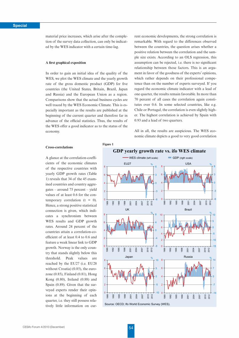
54CESifo Forum 4/2013 (December)

Special

material price increases, which arise after the comple-

tion of the survey data collection, can only be indicat-

ed by the WES indicator with a certain time-lag.

A first graphical exposition

In order to gain an initial idea of the quality of the

WES, we plot the WES climate and the yearly growth

rate of the gross domestic product (GDP) for five

countries (the United States, Britain, Brazil, Japan

and Russia) and the European Union as a region.

Comparisons show that the actual business cycles are

well traced by the WES Economic Climate. This is es-

pecially important as the results are published at the

beginning of the current quarter and therefore far in

advance of the official statistics. Thus, the results of

the WES offer a good indicator as to the status of the

economy.

Cross-correlations

A glance at the correlation-coeffi-

cients of the economic climates

of the respective countries with

yearly GDP growth rates (Table

1) reveals that 34 of the 45 exam-

ined countries and country aggre-

gates – around 75 percent – yield

values of at least 0.6 for the con-

temporary correlation (t = 0).

Hence, a strong positive statistical

connection is given, which indi-

cates a synchronism between

WES results and GDP growth

rates. Around 24 percent of the

countries attain a correlation-co-

efficient of at least 0.4 to 0.6 and

feature a weak linear link to GDP

growth. Norway is the only coun-

try that stands slightly below this

threshold. Peak values are

reached by the EU27 (i.e. EU28

without Croatia) (0.85), the euro-

zone (0.85), Finland (0.81), Hong

Kong (0.80), Ireland (0.88) and

Spain (0.89). Given that the sur-

veyed experts render their opin-

ions at the beginning of each

quarter, i.e. they still possess rela-

tively little information on cur-

rent economic developments, the strong correlation is

remarkable. With regard to the differences observed

between the countries, the question arises whether a

positive relation between the correlation and the sam-

ple size exists. According to an OLS regression, this

assumption can be rejected, i.e. there is no significant

relationship between those factors. This is an argu-

ment in favor of the goodness of the experts’ opinions,

which rather depends on their professional compe-

tence than on the number of experts surveyed. If you

regard the economic climate indicator with a lead of

one quarter, the results remain favorable. In more than

70 percent of all cases the correlation again consti-

tutes over 0.6. In some selected countries, like e.g.

Chile or Portugal, the correlation is even slightly high-

er. The highest correlation is achieved by Spain with

0.93 and a lead of two quarters.

All in all, the results are auspicious. The WES eco-

nomic climate depicts a good to very good correlation

0

2

4

6

819

89

1992

1995

1998

2001

2004

2007

2010

2012

-6

-3

0

3

6

0

2

4

6

8

10

1989

1992

1995

1998

2001

2004

2007

2010

2012

-15

-10

-5

0

5

10

0

2

4

6

8

1989

1992

1995

1998

2001

2004

2007

2010

2012

-6

-3

0

3

6

0

2

4

6

8

1989

1992

1995

1998

2001

2004

2007

2010

2012

-8

-4

0

4

8

GDP yearly growth rate vs. ifo WES climate

0

2

4

6

8

1989

1992

1995

1998

2001

2004

2007

2010

2012

-10

-5

0

5

10

0

2

4

6

8

1989

1992

1995

1998

2001

2004

2007

2010

2012

-14

-7

0

7

14

Source: OECD; Ifo World Economic Survey (WES).

Japan

WES climate (left scale) GDP (rigth scale)

USAEU27

BrazilUK

Russia

%%

%%

%%

Figure 1

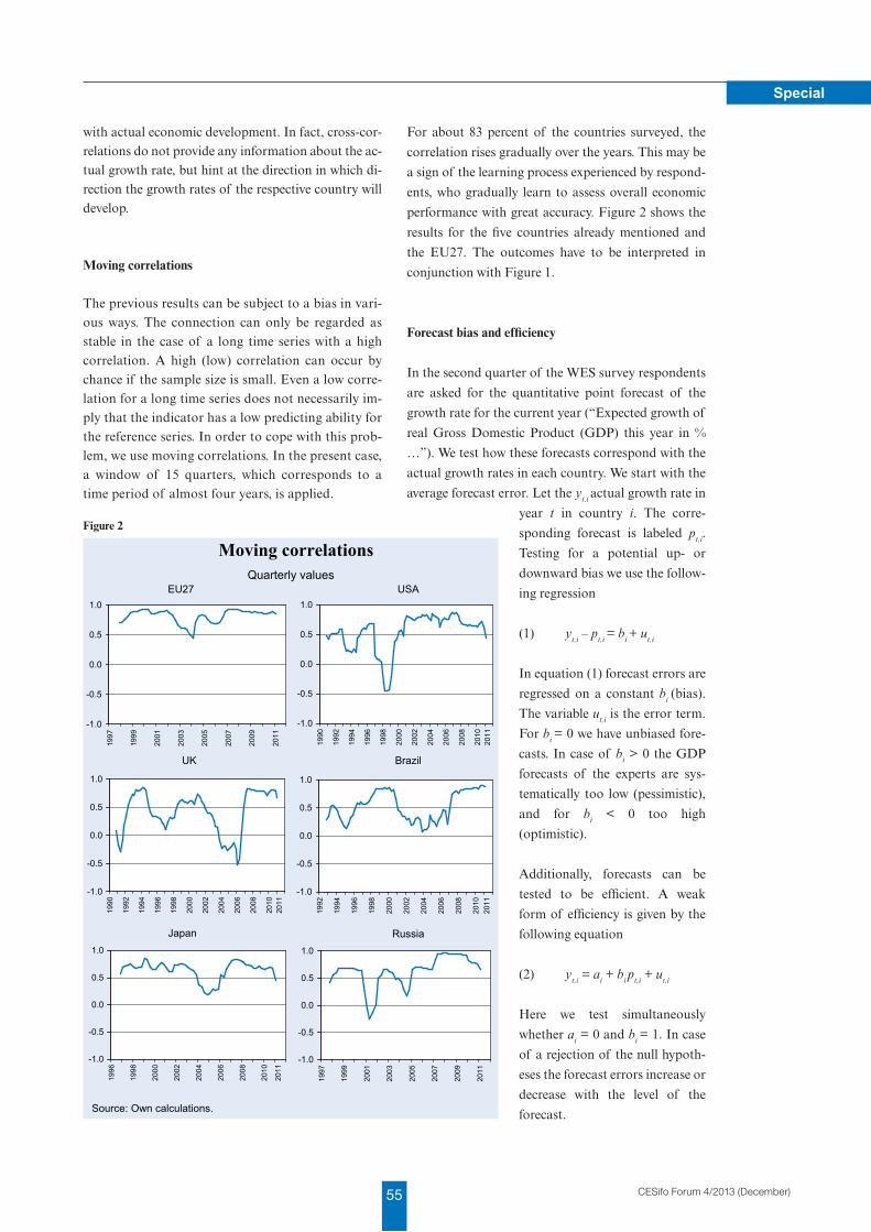
55 CESifo Forum 4/2013 (December)

Special

with actual economic development. In fact, cross-cor-relations do not provide any information about the ac-tual growth rate, but hint at the direction in which di-rection the growth rates of the respective country will develop.

Moving correlations

The previous results can be subject to a bias in vari-ous ways. The connection can only be regarded as stable in the case of a long time series with a high correlation. A high (low) correlation can occur by chance if the sample size is small. Even a low corre-lation for a long time series does not necessarily im-ply that the indicator has a low predicting ability for the reference series. In order to cope with this prob-lem, we use moving correlations. In the present case, a window of 15 quarters, which corresponds to a time period of almost four years, is applied.

For about 83 percent of the countries surveyed, the

correlation rises gradually over the years. This may be

a sign of the learning process experienced by respond-

ents, who gradually learn to assess overall economic

performance with great accuracy. Figure 2 shows the

results for the five countries already mentioned and

the EU27. The outcomes have to be interpreted in

conjunction with Figure 1.

Forecast bias and efficiency

In the second quarter of the WES survey respondents

are asked for the quantitative point forecast of the

growth rate for the current year (“Expected growth of

real Gross Domestic Product (GDP) this year in %

…”). We test how these forecasts correspond with the

actual growth rates in each country. We start with the

average forecast error. Let the yt,i actual growth rate in

year t in country i. The corre-

sponding forecast is labeled pt,i.

Testing for a potential up- or

downward bias we use the follow-

ing regression

(1) yt,i – pt,i = bi + ut,i

In equation (1) forecast errors are

regressed on a constant bi (bias).

The variable ut,i is the error term.

For bi = 0 we have unbiased fore-

casts. In case of bi > 0 the GDP

forecasts of the experts are sys-

tematically too low (pessimistic),

and for bi  <  0 too high

(optimistic).

Additionally, forecasts can be

tested to be efficient. A weak

form of efficiency is given by the

following equation

(2) yt,i = ai + bi pt,i + ut,i

Here we test simultaneously

whether ai = 0 and bi = 1. In case

of a rejection of the null hypoth-

eses the forecast errors increase or

decrease with the level of the

forecast.

-1.0

-0.5

0.0

0.5

1.0

1990

1992

1994

1996

1998

2000

2002

2004

2006

2008

2010

2011

-1.0

-0.5

0.0

0.5

1.0

1992

1994

1996

1998

2000

2002

2004

2006

2008

2010

2011

-1.0

-0.5

0.0

0.5

1.0

1997

1999

2001

2003

2005

2007

2009

2011

-1.0

-0.5

0.0

0.5

1.0

1990

1992

1994

1996

1998

2000

2002

2004

2006

2008

2010

2011

Moving correlations

-1.0

-0.5

0.0

0.5

1.0

1996

1998

2000

2002

2004

2006

2008

2010

2011

-1.0

-0.5

0.0

0.5

1.0

1997

1999

2001

2003

2005

2007

2009

2011

Source: Own calculations.

Japan

USAEU27

BrazilUK

Russia

Quarterly values

Figure 2

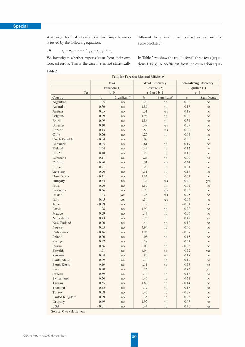
56CESifo Forum 4/2013 (December)

Special

A stronger form of efficiency (semi-strong efficiency) is tested by the following equation:

(3) yt,i – pt,i = ai + ci(yt–1,i – pt–1,i) + ut,i

We investigate whether experts learn from their own forecast errors. This is the case if ci is not statistically

different from zero. The forecast errors are not

autocorrelated.

In Table 2 we show the results for all three tests (equa-

tions 1 to 3). A coefficient from the estimation equa-

Table 2 Tests for Forecast Bias and Efficiency

Bias Weak Efficiency Semi-strong Efficiency Equation (1) Equation (2) Equation (3)

Test b=0 a=0 und b=1 c=0 Country b Significant? b Significant? c Significant? Argentina 1.05 no 1.29 no 0.32 no

Australia 0.36 no 0.89 no – 0.18 no Austria 0.35 no 1.31 yes 0.18 no Belgium 0.09 no 0.96 no – 0.32 no

Brazil 0.09 no 0.86 no – 0.34 no Bulgaria 0.10 no 1.49 yes 0.09 no Canada – 0.13 no 1.50 yes 0.32 no Chile 0.76 no 1.25 no 0.04 no

Czech Republic – 0.04 no 1.08 no 0.36 no Denmark – 0.35 no 1.61 no 0.19 no Estland 1.04 no 1.49 no 0.32 no

EU-27 0.10 no 1.29 no 0.16 no Eurozone – 0.11 no 1.26 no 0.00 no Finland – 0.40 no 1.51 yes 0.24 no France – 0.21 no 1.23 no 0.04 no

Germany 0.20 no 1.31 no 0.16 no Hong Kong – 0.11 no 0.92 no 0.01 no Hungary – 0.64 no 1.34 yes 0.42 yes

India 0.26 no 0.87 no – 0.02 no Indonesia 0.56 no 1.20 yes 0.03 no Ireland 1.33 yes 1.28 yes 0.25 no

Italy – 0.45 yes 1.34 yes – 0.06 no Japan – 0.09 no 1.19 no – 0.01 no Latvia 1.28 no 0.90 no 0.32 no Mexico 0.29 no 1.43 no – 0.05 no

Netherlands 0.43 no 1.25 no 0.42 yes New Zealand 0.30 no 1.44 no 0.12 no Norway – 0.05 no 0.94 no 0.40 no

Philippines – 0.16 no 0.96 no – 0.07 no Poland 0.30 no 1.05 no 0.15 no Portugal 0.32 no 1.38 no 0.23 no Russia 0.66 no 1.00 no – 0.05 no

Slovakia 1.01 no 0.94 no 0.32 yes Slovenia – 0.04 no 1.80 yes 0.18 no South Africa 0.09 no 1.33 no 0.17 no

South Korea 0.59 no 1.11 no – 0.33 no Spain 0.20 no 1.26 no 0.42 yes Sweden 0.59 no 1.16 no 0.13 no Switzerland 0.20 no 1.40 no 0.21 no

Taiwan 0.55 no 0.89 no – 0.14 no Thailand – 0.15 no 1.17 no 0.18 no Turkey 0.38 no 1.45 no – 0.27 no

United Kingdom 0.39 no 1.35 no 0.35 no Uruguay 0.69 no 0.92 no 0.06 no USA – 0.01 no 1.44 no 0.46 yes

Source: Own calculations.

Table 2

57 CESifo Forum 4/2013 (December)

Special

tion is reported for each country and test. Furthermore,

we state, whether the null hypotheses can be rejected

or not. In case of a ‘no’, the null hypothesis cannot be

rejected. This is the desired result.

As far as potential forecasting biases are concerned,

the results are very good. In 32 out of 45 cases the av-

erage forecast error is smaller than 0.5 percentage

points. For some countries like the United States,

Czech Republic, Japan or the EU27, the forecast is

quite close to the actual value. The forecasts only dif-

fer systematically from the realized values in two cas-

es, namely Ireland and Italy.

Column 3 contains the results from equation (2),

whether the biases increase or diminish with the fore-

cast itself. The hypothesis that relatively high forecasts

are too high or too low, and vice versa can be rejected

for a majority of countries. Forecast errors only in-

crease with the level of forecasts for Bulgaria, Finland,

Indonesia, Ireland, Italy, Canada, Austria, Slovenia

and Uruguay.

Semi-strong efficiency is fulfilled for almost 90 percent

of investigated countries. Thus country experts use all

current available information and learn from their

past mistakes. The errors are only autocorrelated for

the Netherlands, Slovakia, Spain, Hungary and the

United States.

Summary

The results show that the Ifo economic climate is a re-

liable indicator for assessing the current and upcom-

ing economic development of a country. Occasional

deviances from GDP are unsurprising, as the experts

surveyed who assess the current situation and future

developments have to monitor many factors like infla-

tion, the labor market, political stability, financing

conditions etc. Basically, however, expert opinions

point in the right direction and can reliably detect

turning points. Moreover, the quantitative GDP point

forecasts are unbiased and efficient for the majority of

investigated countries. This means that WES experts

on average have a fairly good idea of yearly growth

rate in the second quarter.

It is worth mentioning that the relationships between

the opinion of experts and actual economic develop-

ments have improved over time. This indicates some

learning effects. Another advantage is that the quality

of the indicators does not depend on the number of participating experts.

References

Abberger, K., M. Frey, M. Kesina and A. Stangl (2009), “Indikatoren für die globale Konjunktur”, ifo Schnelldienst 62(16), 32–41.

Brand, D., G. Nerb, F.J. Klein and K. Stock (1990), “Construction and Performance of a World Economy Leading Indicator”, in: Oppenländer, K.H. and G. Poser (eds.), Business Cycle Surveys with Special Reference to Pacific Basin Economies. Papers presented at the 19th CIRET Conference, Proceedings, Osaka 1989, Aldershot: Edward Elgar, 249–290,

Brand, D. and L. Pouquet (1993), The Explanatory and Forecasting Power of the Economic Survey International, CIRET Studien 49, Munich: Ifo Institute.

Haupt, H. and S. Waller (2004), “Informationsgehalt von WES-Daten zur Inflationsprognose”, in: Goldrian, G. (ed.): Handbuch der umfragebasierten Konjunkturforschung, ifo Beiträge zur Wirtschaftsforschung 15, Munich.

Henzel, S. and T. Wollmershäuser (2005), “An Alternative to the Carlson-Parkin Method for the Quantification of Qualitative Inflation Expectations: Evidence from the Ifo World Economic Survey”, Journal of Business Cycle Measurement and Analysis 2, 321–352.

Henzel, S. and T. Wollmershäuser (2006), The New Keynesian Phillips Curve and the Role of Expectations: Evidence from the Ifo World Economic Survey, CESifo Working Paper 1694.

Hülseweig, O., J. Mayr and T. Wollmershäuser (2008), Forecasting Euro Area Real GDP: Optimal Pooling of Information, CESifo Working Paper 2371.

Nerb, G. and J. Plenk (2013), “ifo Weltwirtschaftsklima trübt sich leicht ein – Ergebnisse des 121. World Economic Survey (WES) für das dritte Quartal 2013”, ifo Schnelldienst 66(16), 35–46.

Nerb, G., J. Plenk and K. Wohlrabe and T. Wollmershäuser (2013), “CESifo World Economic Survey August 2013”, CESifo World Economic Survey 12(3).

Stangl A. (2004), “World Economic Survey: Umfragen des ifo Instituts; Konzeption, Repräsentation, Qualitätssicherung”, in: Goldrian, G. (ed.), Handbuch der umfragebasierten Konjunkturforschung, Munich: Ifo Institute, 140–147.

Stangl A. (2007a), “Internet Business Tendency Surveys”, OECD Journal of Business Cycle Measurement and Analysis 3, 387–400.

Stangl A. (2007b), “Ifo World Economic Survey Micro Data”, Journal of Applied Social Science Studies 127, 487–496.

Stangl A. (2009), Essays on the Measurement of Economic Expectations, Munich Dissertations in Economics 9823, University of Munich, Department of Economics.

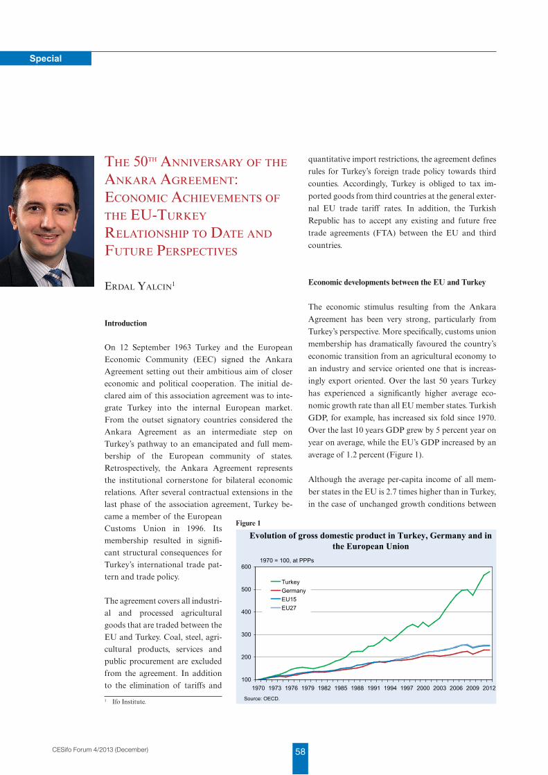
58CESifo Forum 4/2013 (December)

Special

The 50Th AnniversAry of The AnkArA AgreemenT: economic AchievemenTs of The eU-TUrkey relATionship To DATe AnD fUTUre perspecTives

erDAl yAlcin1

Introduction

On 12 September 1963 Turkey and the European

Economic Community (EEC) signed the Ankara

Agreement setting out their ambitious aim of closer

economic and political cooperation. The initial de-

clared aim of this association agreement was to inte-

grate Turkey into the internal European market.

From the outset signatory countries considered the

Ankara Agreement as an intermediate step on

Turkey’s pathway to an emancipated and full mem-

bership of the European community of states.

Retrospectively, the Ankara Agreement represents

the institutional cornerstone for bilateral economic

relations. After several contractual extensions in the

last phase of the association agreement, Turkey be-

came a member of the European

Customs Union in 1996. Its

membership resulted in signifi-

cant structural consequences for

Turkey’s international trade pat-

tern and trade policy.

The agreement covers all industri-

al and processed agricultural

goods that are traded between the

EU and Turkey. Coal, steel, agri-

cultural products, services and

public procurement are excluded

from the agreement. In addition

to the elimination of tariffs and

1 Ifo Institute.

quantitative import restrictions, the agreement defines

rules for Turkey’s foreign trade policy towards third

counties. Accordingly, Turkey is obliged to tax im-

ported goods from third countries at the general exter-

nal EU trade tariff rates. In addition, the Turkish

Republic has to accept any existing and future free

trade agreements (FTA) between the EU and third

countries.

Economic developments between the EU and Turkey

The economic stimulus resulting from the Ankara

Agreement has been very strong, particularly from

Turkey’s perspective. More specifically, customs union

membership has dramatically favoured the country’s

economic transition from an agricultural economy to

an industry and service oriented one that is increas-

ingly export oriented. Over the last 50 years Turkey

has experienced a significantly higher average eco-

nomic growth rate than all EU member states. Turkish

GDP, for example, has increased six fold since 1970.

Over the last 10 years GDP grew by 5 percent year on

year on average, while the EU’s GDP increased by an

average of 1.2 percent (Figure 1).

Although the average per-capita income of all mem-

ber states in the EU is 2.7 times higher than in Turkey,

in the case of unchanged growth conditions between

100

200

300

400

500

600

1970 1973 1976 1979 1982 1985 1988 1991 1994 1997 2000 2003 2006 2009 2012

TurkeyGermanyEU15EU27

Evolution of gross domestic product in Turkey, Germany and in the European Union

Source: OECD.

1970 = 100, at PPPs

Figure 1

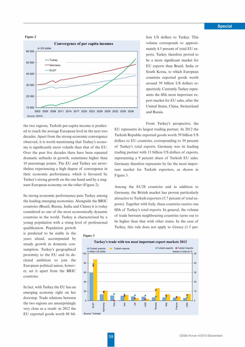
59 CESifo Forum 4/2013 (December)

Special

the two regions, Turkish per-capita income is predict-

ed to reach the average European level in the next two

decades. Apart from the strong economic convergence

observed, it is worth mentioning that Turkey’s econo-

my is significantly more volatile than that of the EU.

Over the past five decades there have been repeated

dramatic setbacks in growth, sometimes higher than

10 percentage points. The EU and Turkey are never-

theless experiencing a high degree of convergence in

their economic performance, which is favoured by

Turkey’s strong growth on the one hand and by a stag-

nant European economy on the other (Figure 2).

Its strong economic performance puts Turkey among

the leading emerging economies. Alongside the BRIC

countries (Brazil, Russia, India and China) it is today

considered as one of the most economically dynamic

countries in the world. Turkey is characterized by a

young population with a rising level of professional

qualification. Population growth

is predicted to be stable in the

years ahead, accompanied by

steady growth in domestic con-

sumption. Turkey’s geographical

proximity to the EU and its de-

clared ambition to join the

European political union, howev-

er, set it apart from the BRIC

countries.

In fact, with Turkey the EU has an

emerging economy right on her

doorstep. Trade relations between

the two regions are unsurprisingly

very close as a result: in 2012 the

EU exported goods worth 88 bil-

lion US dollars to Turkey. This

volume corresponds to approxi-

mately 4.5 percent of total EU ex-

ports. Turkey therefore proved to

be a more significant market for

EU exports than Brazil, India or

South Korea, to which European

countries exported goods worth

around 59 billion US dollars re-

spectively. Currently Turkey repre-

sents the fifth most important ex-

port market for EU sales, after the

United States, China, Switzerland

and Russia.

From Turkey’s perspective, the

EU represents its largest trading partner. In 2012 the

Turkish Republic exported goods worth 59 billion US

dollars to EU countries, corresponding to 39 percent

of Turkey’s total exports. Germany was its leading

trading partner with 13 billion US dollars of exports,

representing a 9 percent share of Turkish EU sales.

Germany therefore represents by far the most impor-

tant market for Turkish exporters, as shown in

Figure 3.

Among the EU28 countries and in addition to

Germany, the British market has proven particularly

attractive to Turkish exporters (5.7 percent of total ex-

ports). Together with Italy, these countries receive one

fifth of Turkey’s total exports. In general, the volume

of trade between neighbouring countries turns out to

be higher than that with other states. In the case of

Turkey, this rule does not apply to Greece (1.5 per-

10 000

20 000

30 000

40 000

50 000

60 000

2002 2005 2008 2011 2014 2017 2020 2023 2026 2029 2032 2035 2038

Turkey

Germany

EU27

Convergence of per capita incomes

Source: OECD.

in US dollar

Figure 2

0

20

40

60

80

100

EU

27

Ger

man

y

Iraq

Iran

UK

UA

E

Rus

sia

Italy

Fran

ce

US

A

0

10

20

30

40

50

Turkish exports Turkish imports

Turkey's trade with ten most important export markets 2012

in billion US dollar

Source: Turkstat.

shares in total as %Turkish exports Turkish imports

Figure 3

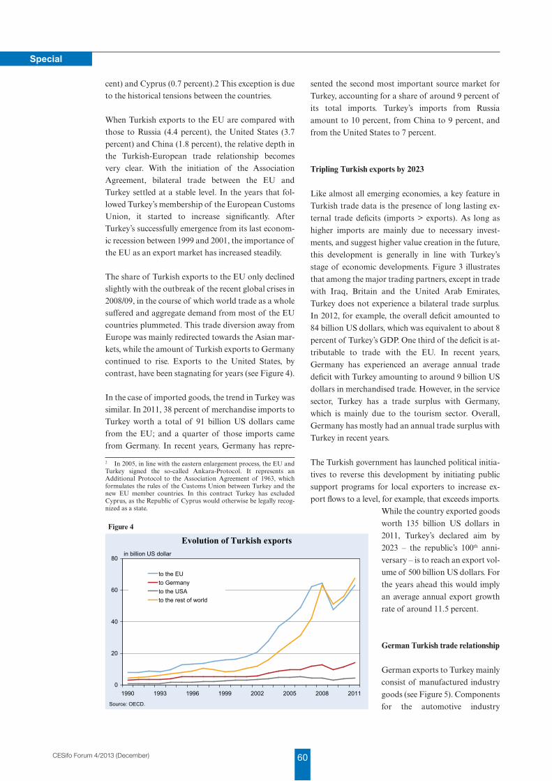
60CESifo Forum 4/2013 (December)

Special

cent) and Cyprus (0.7 percent).2 This exception is due to the historical tensions between the countries.

When Turkish exports to the EU are compared with those to Russia (4.4 percent), the United States (3.7 percent) and China (1.8 percent), the relative depth in the Turkish-European trade relationship becomes very clear. With the initiation of the Association Agreement, bilateral trade between the EU and Turkey settled at a stable level. In the years that fol-lowed Turkey’s membership of the European Customs Union, it started to increase significantly. After Turkey’s successfully emergence from its last econom-ic recession between 1999 and 2001, the importance of the EU as an export market has increased steadily.

The share of Turkish exports to the EU only declined slightly with the outbreak of the recent global crises in 2008/09, in the course of which world trade as a whole suffered and aggregate demand from most of the EU countries plummeted. This trade diversion away from Europe was mainly redirected towards the Asian mar-kets, while the amount of Turkish exports to Germany continued to rise. Exports to the United States, by contrast, have been stagnating for years (see Figure 4).

In the case of imported goods, the trend in Turkey was similar. In 2011, 38 percent of merchandise imports to Turkey worth a total of 91 billion US dollars came from the EU; and a quarter of those imports came from Germany. In recent years, Germany has repre-

2 In 2005, in line with the eastern enlargement process, the EU and Turkey signed the so-called Ankara-Protocol. It represents an Additional Protocol to the Association Agreement of 1963, which formulates the rules of the Customs Union between Turkey and the new EU member countries. In this contract Turkey has excluded Cyprus, as the Republic of Cyprus would otherwise be legally recog-nized as a state.

sented the second most important source market for

Turkey, accounting for a share of around 9 percent of

its total imports. Turkey’s imports from Russia

amount to 10 percent, from China to 9 percent, and

from the United States to 7 percent.

Tripling Turkish exports by 2023

Like almost all emerging economies, a key feature in

Turkish trade data is the presence of long lasting ex-

ternal trade deficits (imports > exports). As long as

higher imports are mainly due to necessary invest-

ments, and suggest higher value creation in the future,

this development is generally in line with Turkey’s

stage of economic developments. Figure 3 illustrates

that among the major trading partners, except in trade

with Iraq, Britain and the United Arab Emirates,

Turkey does not experience a bilateral trade surplus.

In 2012, for example, the overall deficit amounted to

84 billion US dollars, which was equivalent to about 8

percent of Turkey’s GDP. One third of the deficit is at-

tributable to trade with the EU. In recent years,

Germany has experienced an average annual trade

deficit with Turkey amounting to around 9 billion US

dollars in merchandised trade. However, in the service

sector, Turkey has a trade surplus with Germany,

which is mainly due to the tourism sector. Overall,

Germany has mostly had an annual trade surplus with

Turkey in recent years.

The Turkish government has launched political initia-

tives to reverse this development by initiating public

support programs for local exporters to increase ex-

port flows to a level, for example, that exceeds imports.

While the country exported goods

worth 135 billion US dollars in

2011, Turkey’s declared aim by

2023 – the republic’s 100th anni-

versary – is to reach an export vol-

ume of 500 billion US dollars. For

the years ahead this would imply

an average annual export growth

rate of around 11.5 percent.

German Turkish trade relationship

German exports to Turkey mainly

consist of manufactured industry

goods (see Figure 5). Components

for the automotive industry

0

20

40

60

80

1990 1993 1996 1999 2002 2005 2008 2011

to the EUto Germanyto the USAto the rest of world

Evolution of Turkish exports

Source: OECD.

in billion US dollar

Figure 4

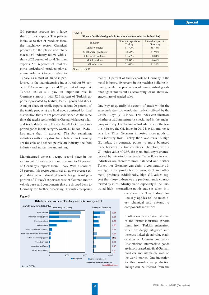
61 CESifo Forum 4/2013 (December)

Special

(30  percent) account for a large

share of these exports. This pattern

is similar to that of products from

the machinery sector. Chemical

products for the plastic and phar-

maceutical industry follow with a

share of 22 percent of total German

exports. At 0.6 percent of total ex-

ports, agricultural products play a

minor role in German sales to

Turkey, as almost all trade is per-

formed in the manufacturing industry (about 98 per-

cent of German exports and 96 percent of imports).

Turkish textiles still play an important role in

Germany’s imports: with 32.5 percent of Turkish ex-

ports represented by textiles, leather goods and shoes.

A major share of textile exports (about 90 percent of

the textile products) are final goods destined for final

distribution that are not processed further. At the same

time, the textile sector exhibits Germany’s largest bilat-

eral trade deficit with Turkey. In 2011 Germany im-

ported goods in this category worth 4.2 billion US dol-

lars more than it exported. The few remaining

industries with a negative trade balance in Germany

are the coke and refined petroleum industry, the food

industry and agriculture and mining.

Manufactured vehicles occupy second place in the

ranking of Turkish exports and account for 19 percent

of Germany’s imports from Turkey. With a share of

58 percent, this sector comprises an above-average ex-

port share of semi-finished goods. A significant pro-

portion of Turkey’s exports consist of German motor

vehicle parts and components that are shipped back to

Germany for further processing. Turkish enterprises

realize 11 percent of their exports to Germany in the

metal industry, 10 percent in the machine building in-

dustry; while the production of semi-finished goods

once again stands out as accounting for an above-av-

erage share of traded sales.

One way to quantify the extent of trade within the

same industry (intra-industry trade) is offered by the

Grubel-Lloyd (GL) index. This index can illustrate

whether a trading partner is specialized in the under-

lying industry. For German-Turkish trade in the tex-

tile industry the GL-index in 2012 is 0.13, and hence

very low. Thus, Germany imported more goods in

this industry from Turkey than vice versa. A high

GL-index, by contrast, points to more balanced

trade between the two countries. Therefore, with a

GL-index value of 0.93, the metal industry is charac-

terised by intra-industry trade. Trade flows in such

industries are therefore more balanced and neither

Turkey nor Germany can claim a comparative ad-

vantage in the production of iron, steel and other

metal products. Additionally, high GL-values sug-

gest that those industries are predominantly charac-

terized by intra-industry trade, especially if the illus-

trated high intermediate goods trade is taken into

consideration. This finding par-

ticularly applies to the machin-

ery, chemical and automotive

components industries.

In other words, a substantial share

of the former industries’ exports

stems from Turkish enterprises,

which are deeply integrated into

the cross-linked global value-chain

creation of German companies.

Cost-efficient intermediate goods

are incorporated into final German

products and ultimately sold on

the world market. One indication

for this cross-border production

linkage can be inferred from the

0 4000 8000

Mining and quarrying

Agriculture and fishing

Products of wood

Textiles and wearing apparel

Food prod., beverages and tobacco

Wood, publishing and printing

Metal products

Chemical products

Machinery and equipment

Motor vehicles

Final goods

0 4000

0.6

0.45

0.14

0.13

0.67

0.14

0.93

0.39

0.34

0.54

Semi-finished goods

Turkey to GermanyGermany to Turkey

Indicator for intra-industy trade: Grubel-Lloyd-IndexSource: OECD.

Bilateral exports of Turkey and Germany 2011Exports in million US dollar

Figure 5

Table 1 Share of unfinished goods in total trade (four selected industries)

Industry German exports to Turkey

Turkish exports to Germany

Motor vehicles 31.79% 58.48% Mechanical products 32.61% 57.92% Chemical products 81.63% 88.84%

Metal products 89.84% 86.48% All industries 51.01% 41.31%

Source: OECD

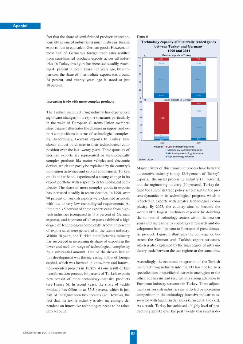
62CESifo Forum 4/2013 (December)

Special

fact that the share of semi-finished products in techno-

logically advanced industries is much higher in Turkish

exports than in equivalent German goods. However, al-

most half of Germany’s foreign trade sales resulted

from semi-finished products exports across all indus-

tries. In Turkey this figure has increased steadily, reach-

ing 41 percent in recent years. Ten years ago, by com-

parison, the share of intermediate exports was around

24 percent, and twenty years ago it stood at just

18 percent.

Increasing trade with more complex products

The Turkish manufacturing industry has experienced

significant changes in its export structure, particularly

in the wake of European Customs Union member-

ship. Figure 6 illustrates the changes in import and ex-

port compositions in terms of technological complex-

ity. Accordingly, German exports to Turkey have

shown almost no change in their technological com-

position over the last twenty years. Three quarters of

German exports are represented by technologically

complex products like motor vehicles and electronic

devices, which can partly be explained by the country’s

innovation activities and capital endowment. Turkey,

on the other hand, experienced a strong change in its

export portfolio with respect to its technological com-

plexity. The share of more complex goods in exports

has increased steadily in recent decades. In 1990, over

90 percent of Turkish exports were classified as goods

with low or very low technological requirements. At

that time 3.5 percent of these exports came from high-

tech industries (compared to 11.9 percent of German

exports), and 6 percent of all exports exhibited a high

degree of technological complexity. About 65 percent

of export sales were generated in the textile industry.

Within 20 years, the Turkish manufacturing industry

has succeeded in increasing its share of exports in the

lower and medium range of technological complexity

by a substantial amount. One of the drivers behind

this development was the increasing inflow of foreign

capital, which was invested in know-how and innova-

tion-oriented projects in Turkey. As one result of this

transformation process, 60 percent of Turkish exports

now consist of more technology-intensive products

(see Figure 6). In recent years, the share of textile

products has fallen to at 32.5 percent, which is just

half of the figure seen two decades ago. However, the

fact that the textile industry is also increasingly de-

pendent on innovative technologies needs to be taken

into account.

Major drivers of this transition process have been the

automotive industry (today 18.4 percent of Turkey’s

exports), the metal processing industry (11 percent),

and the engineering industry (10 percent). Turkey de-

fined the aim of its trade policy as to maintain the pre-

sent dynamics in its technological progress, which is

reflected in exports with greater technological com-

plexity. By 2023, the country aims to become the

world’s fifth largest machinery exporter by doubling

the number of technology centers within the next ten

years and increasing its spending on research and de-

velopment from 1 percent to 3 percent of gross domes-

tic product. Figure 6 illustrates the convergence be-

tween the German and Turkish export structure,

which is also explained by the high degree of intra-in-

dustry trade between the two regions at the same time.

Accordingly, the economic integration of the Turkish

manufacturing industry into the EU has not led to a

specialization in specific industries in one region or the

other, but has instead resulted in a strong adaption to

European industry structure in Turkey. These adjust-

ments in Turkish industries are reflected by increasing

competition in the technology-intensive industries as-

sociated with high firm dynamics (firm entry and exit).

As a result, Turkey has achieved a highly level of pro-

ductivity growth over the past twenty years and is de-

11.91 11.60

66.75 68.00

14.63 13.01

6.71 7.39

0

20

40

60

80

100

Technology capacity of bilaterally traded goods between Turkey and Germany

1990 and 2011

6.785.99

53.27

6.47

33.35

84.00

6.60

3.550

20

40

60

80

100

1990 2011

Low technology industriesMedium-low technology industriesMedium-high technology industriesHigh technology industries

German exports to Turkey

Industries

Source: OECD.

Turkish exports to Germany

%

%

Figure 6

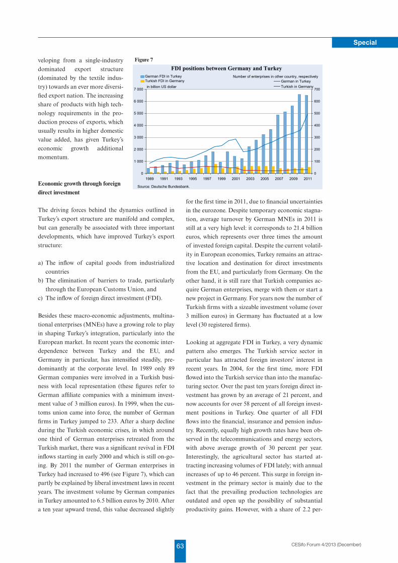
63 CESifo Forum 4/2013 (December)

Special

veloping from a single-industry

dominated export structure

(dominated by the textile indus-

try) towards an ever more diversi-

fied export nation. The increasing

share of products with high tech-

nology requirements in the pro-

duction process of exports, which

usually results in higher domestic

value added, has given Turkey’s

economic growth additional

momentum.

Economic growth through foreign direct investment

The driving forces behind the dynamics outlined in

Turkey’s export structure are manifold and complex,

but can generally be associated with three important

developments, which have improved Turkey’s export

structure:

a) The inflow of capital goods from industrialized

countries

b) The elimination of barriers to trade, particularly

through the European Customs Union, and

c) The inflow of foreign direct investment (FDI).

Besides these macro-economic adjustments, multina-

tional enterprises (MNEs) have a growing role to play

in shaping Turkey’s integration, particularly into the

European market. In recent years the economic inter-

dependence between Turkey and the EU, and

Germany in particular, has intensified steadily, pre-

dominantly at the corporate level. In 1989 only 89

German companies were involved in a Turkish busi-

ness with local representation (these figures refer to

German affiliate companies with a minimum invest-

ment value of 3 million euros). In 1999, when the cus-

toms union came into force, the number of German

firms in Turkey jumped to 233. After a sharp decline

during the Turkish economic crises, in which around

one third of German enterprises retreated from the

Turkish market, there was a significant revival in FDI

inflows starting in early 2000 and which is still on-go-

ing. By 2011 the number of German enterprises in

Turkey had increased to 496 (see Figure 7), which can

partly be explained by liberal investment laws in recent

years. The investment volume by German companies

in Turkey amounted to 6.5 billion euros by 2010. After

a ten year upward trend, this value decreased slightly

for the first time in 2011, due to financial uncertainties

in the eurozone. Despite temporary economic stagna-

tion, average turnover by German MNEs in 2011 is

still at a very high level: it corresponds to 21.4 billion

euros, which represents over three times the amount

of invested foreign capital. Despite the current volatil-

ity in European economies, Turkey remains an attrac-

tive location and destination for direct investments

from the EU, and particularly from Germany. On the

other hand, it is still rare that Turkish companies ac-

quire German enterprises, merge with them or start a

new project in Germany. For years now the number of

Turkish firms with a sizeable investment volume (over

3 million euros) in Germany has fluctuated at a low

level (30 registered firms).

Looking at aggregate FDI in Turkey, a very dynamic

pattern also emerges. The Turkish service sector in

particular has attracted foreign investors’ interest in

recent years. In 2004, for the first time, more FDI

flowed into the Turkish service than into the manufac-

turing sector. Over the past ten years foreign direct in-

vestment has grown by an average of 21 percent, and

now accounts for over 58 percent of all foreign invest-

ment positions in Turkey. One quarter of all FDI

flows into the financial, insurance and pension indus-

try. Recently, equally high growth rates have been ob-

served in the telecommunications and energy sectors,

with above average growth of 30 percent per year.

Interestingly, the agricultural sector has started at-

tracting increasing volumes of FDI lately; with annual

increases of up to 46 percent. This surge in foreign in-

vestment in the primary sector is mainly due to the

fact that the prevailing production technologies are

outdated and open up the possibility of substantial

productivity gains. However, with a share of 2.2 per-

0

1 000

2 000

3 000

4 000

5 000

6 000

7 000

1989 1991 1993 1995 1997 1999 2001 2003 2005 2007 2009 20110

100

200

300

400

500

600

700

German in TurkeyTurkish in Germany

FDI positions between Germany and Turkey

in billion US dollar

Source: Deutsche Bundesbank.

Number of enterprises in other country, respectivelyGerman FDI in TurkeyTurkish FDI in Germany

Figure 7

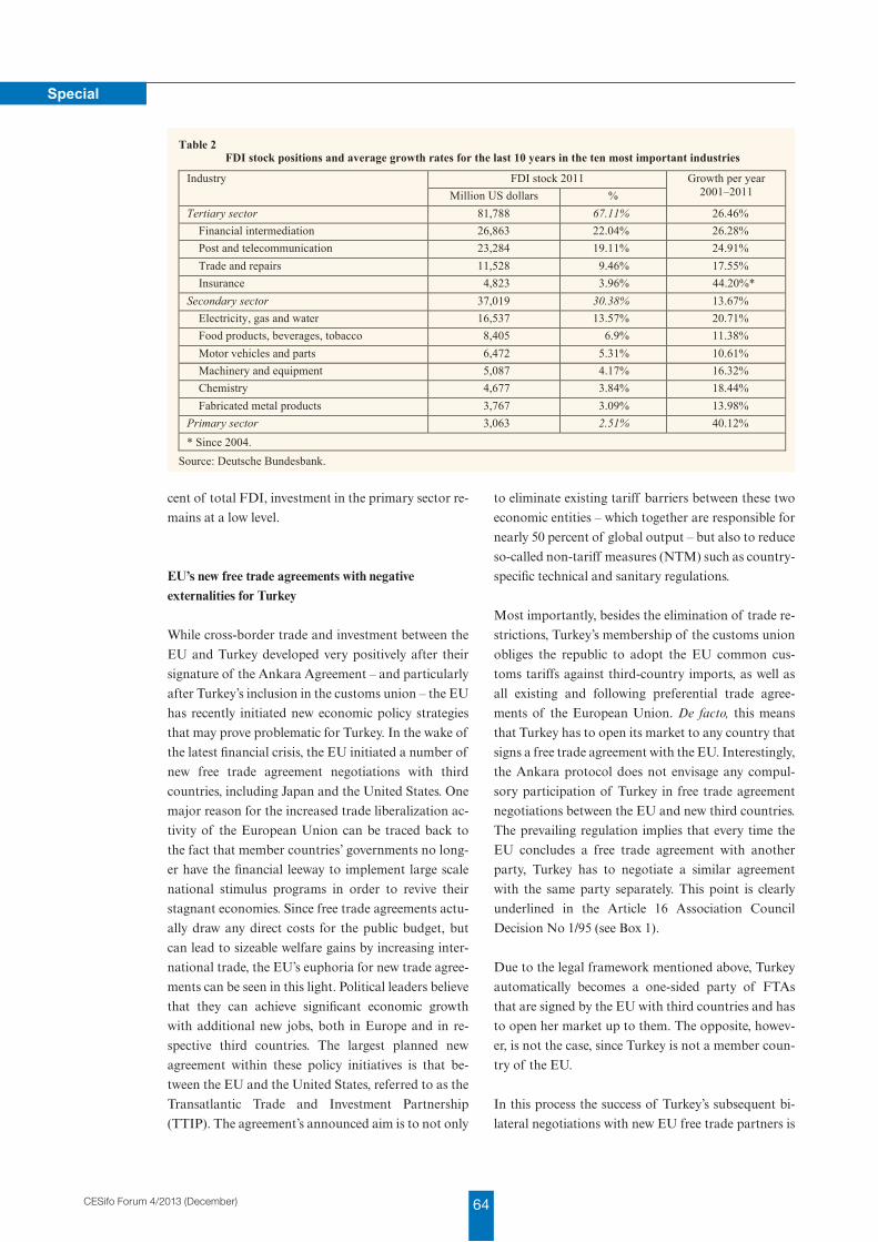
64CESifo Forum 4/2013 (December)

Special

cent of total FDI, investment in the primary sector re-

mains at a low level.

EU’s new free trade agreements with negative externalities for Turkey

While cross-border trade and investment between the

EU and Turkey developed very positively after their

signature of the Ankara Agreement – and particularly

after Turkey’s inclusion in the customs union – the EU

has recently initiated new economic policy strategies

that may prove problematic for Turkey. In the wake of

the latest financial crisis, the EU initiated a number of

new free trade agreement negotiations with third

countries, including Japan and the United States. One

major reason for the increased trade liberalization ac-

tivity of the European Union can be traced back to

the fact that member countries’ governments no long-

er have the financial leeway to implement large scale

national stimulus programs in order to revive their

stagnant economies. Since free trade agreements actu-

ally draw any direct costs for the public budget, but

can lead to sizeable welfare gains by increasing inter-

national trade, the EU’s euphoria for new trade agree-

ments can be seen in this light. Political leaders believe

that they can achieve significant economic growth

with additional new jobs, both in Europe and in re-

spective third countries. The largest planned new

agreement within these policy initiatives is that be-

tween the EU and the United States, referred to as the

Transatlantic Trade and Investment Partnership

(TTIP). The agreement’s announced aim is to not only

to eliminate existing tariff barriers between these two

economic entities – which together are responsible for

nearly 50 percent of global output – but also to reduce

so-called non-tariff measures (NTM) such as country-

specific technical and sanitary regulations.

Most importantly, besides the elimination of trade re-

strictions, Turkey’s membership of the customs union

obliges the republic to adopt the EU common cus-

toms tariffs against third-country imports, as well as

all existing and following preferential trade agree-

ments of the European Union. De facto, this means

that Turkey has to open its market to any country that

signs a free trade agreement with the EU. Interestingly,

the Ankara protocol does not envisage any compul-

sory participation of Turkey in free trade agreement

negotiations between the EU and new third countries.

The prevailing regulation implies that every time the

EU concludes a free trade agreement with another

party, Turkey has to negotiate a similar agreement

with the same party separately. This point is clearly

underlined in the Article 16 Association Council

Decision No 1/95 (see Box 1).

Due to the legal framework mentioned above, Turkey

automatically becomes a one-sided party of FTAs

that are signed by the EU with third countries and has

to open her market up to them. The opposite, howev-

er, is not the case, since Turkey is not a member coun-

try of the EU.

In this process the success of Turkey’s subsequent bi-

lateral negotiations with new EU free trade partners is

Table 2

FDI stock positions and average growth rates for the last 10 years in the ten most important industries

Industry FDI stock 2011 Growth per year 2001–2011 Million US dollars %

Tertiary sector 81,788 67.11% 26.46% Financial intermediation 26,863 22.04% 26.28% Post and telecommunication 23,284 19.11% 24.91% Trade and repairs 11,528 9.46% 17.55% Insurance 4,823 3.96% 44.20%* Secondary sector 37,019 30.38% 13.67% Electricity, gas and water 16,537 13.57% 20.71% Food products, beverages, tobacco 8,405 6.9% 11.38% Motor vehicles and parts 6,472 5.31% 10.61% Machinery and equipment 5,087 4.17% 16.32% Chemistry 4,677 3.84% 18.44% Fabricated metal products 3,767 3.09% 13.98% Primary sector 3,063 2.51% 40.12% * Since 2004.

Source: Deutsche Bundesbank.

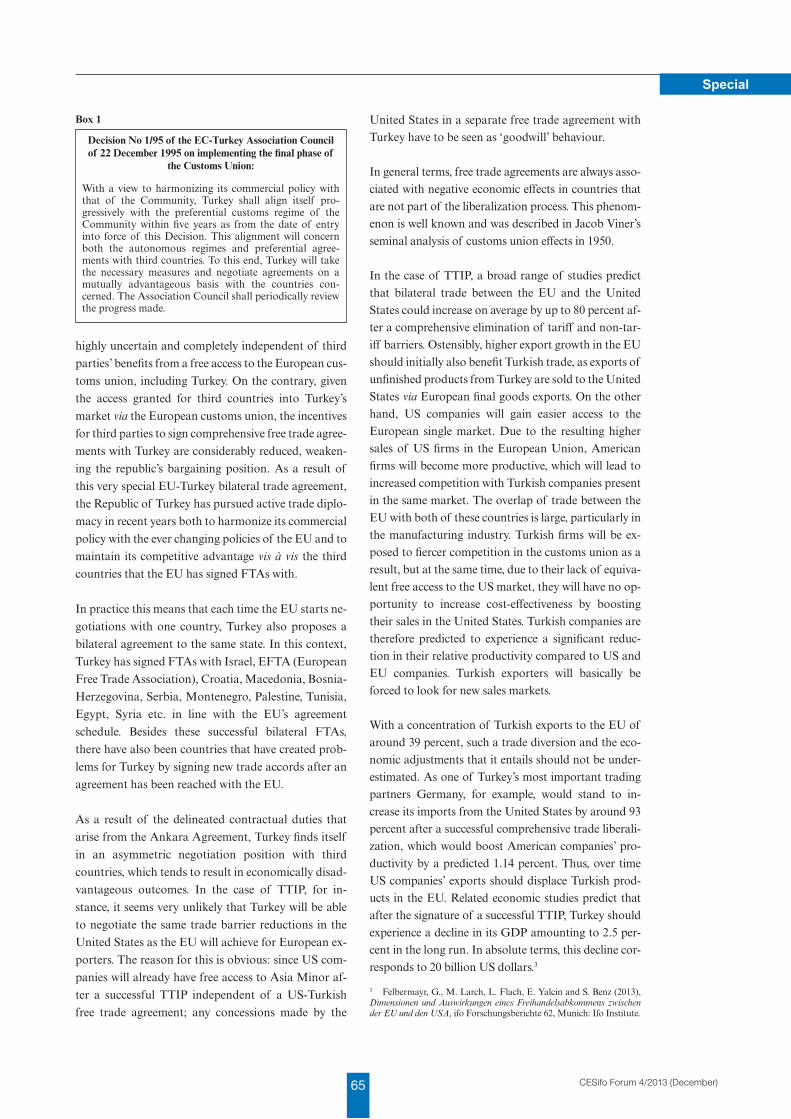
65 CESifo Forum 4/2013 (December)

Special

highly uncertain and completely independent of third

parties’ benefits from a free access to the European cus-

toms union, including Turkey. On the contrary, given

the access granted for third countries into Turkey’s

market via the European customs union, the incentives

for third parties to sign comprehensive free trade agree-

ments with Turkey are considerably reduced, weaken-

ing the republic’s bargaining position. As a result of

this very special EU-Turkey bilateral trade agreement,

the Republic of Turkey has pursued active trade diplo-

macy in recent years both to harmonize its commercial

policy with the ever changing policies of the EU and to

maintain its competitive advantage vis à vis the third

countries that the EU has signed FTAs with.

In practice this means that each time the EU starts ne-

gotiations with one country, Turkey also proposes a

bilateral agreement to the same state. In this context,

Turkey has signed FTAs with Israel, EFTA (European

Free Trade Association), Croatia, Macedonia, Bosnia-

Herzegovina, Serbia, Montenegro, Palestine, Tunisia,

Egypt, Syria etc. in line with the EU’s agreement

schedule. Besides these successful bilateral FTAs,

there have also been countries that have created prob-

lems for Turkey by signing new trade accords after an

agreement has been reached with the EU.

As a result of the delineated contractual duties that

arise from the Ankara Agreement, Turkey finds itself

in an asymmetric negotiation position with third

countries, which tends to result in economically disad-

vantageous outcomes. In the case of TTIP, for in-

stance, it seems very unlikely that Turkey will be able

to negotiate the same trade barrier reductions in the

United States as the EU will achieve for European ex-

porters. The reason for this is obvious: since US com-

panies will already have free access to Asia Minor af-

ter a successful TTIP independent of a US-Turkish

free trade agreement; any concessions made by the

United States in a separate free trade agreement with Turkey have to be seen as ‘goodwill’ behaviour.

In general terms, free trade agreements are always asso-ciated with negative economic effects in countries that are not part of the liberalization process. This phenom-enon is well known and was described in Jacob Viner’s seminal analysis of customs union effects in 1950.

In the case of TTIP, a broad range of studies predict that bilateral trade between the EU and the United States could increase on average by up to 80 percent af-ter a comprehensive elimination of tariff and non-tar-iff barriers. Ostensibly, higher export growth in the EU should initially also benefit Turkish trade, as exports of unfinished products from Turkey are sold to the United States via European final goods exports. On the other hand, US companies will gain easier access to the European single market. Due to the resulting higher sales of US firms in the European Union, American firms will become more productive, which will lead to increased competition with Turkish companies present in the same market. The overlap of trade between the EU with both of these countries is large, particularly in the manufacturing industry. Turkish firms will be ex-posed to fiercer competition in the customs union as a result, but at the same time, due to their lack of equiva-lent free access to the US market, they will have no op-portunity to increase cost-effectiveness by boosting their sales in the United States. Turkish companies are therefore predicted to experience a significant reduc-tion in their relative productivity compared to US and EU companies. Turkish exporters will basically be forced to look for new sales markets.

With a concentration of Turkish exports to the EU of around 39 percent, such a trade diversion and the eco-nomic adjustments that it entails should not be under-estimated. As one of Turkey’s most important trading partners Germany, for example, would stand to in-crease its imports from the United States by around 93 percent after a successful comprehensive trade liberali-zation, which would boost American companies’ pro-ductivity by a predicted 1.14 percent. Thus, over time US companies’ exports should displace Turkish prod-ucts in the EU. Related economic studies predict that after the signature of a successful TTIP, Turkey should experience a decline in its GDP amounting to 2.5 per-cent in the long run. In absolute terms, this decline cor-responds to 20 billion US dollars.3

3 Felbermayr, G., M. Larch, L. Flach, E. Yalcin and S. Benz (2013), Dimensionen und Auswirkungen eines Freihandelsabkommens zwischen der EU und den USA, ifo Forschungsberichte 62, Munich: Ifo Institute.

Decision No 1/95 of the EC-Turkey Association Council of 22 December 1995 on implementing the final phase of

the Customs Union:

With a view to harmonizing its commercial policy with that of the Community, Turkey shall align itself pro-gressively with the preferential customs regime of the Community within five years as from the date of entry into force of this Decision. This alignment will concern both the autonomous regimes and preferential agree-ments with third countries. To this end, Turkey will take the necessary measures and negotiate agreements on a mutually advantageous basis with the countries con-cerned. The Association Council shall periodically review the progress made.

Box 1

66CESifo Forum 4/2013 (December)

Special

In addition, Turkish companies are confronted with a

direct negative effect after the EU signs trade agree-

ments with third parties. With each new trade agree-

ment signed by the EU Turkish companies – particu-

larly in the manufacturing industry – are faced with an

increasing intensification of competition in their do-

mestic market. Simultaneously, if the Turkish

Republic fails to sign an equivalent agreement with

the respective third countries in a timely manner,

Turkey will experience an ever growing trade deficit,

which is already on a very high level (see above).

In fact, most of Turkey’s recent free trade agreements

were not negotiated and motivated by regional eco-

nomic integration efforts, but tend to represent a rou-

tine response to EU negotiations. One example of such

a response is the recent free trade agreement with

South Korea. Negotiations on bilateral trade liberali-

zation between the EU and South Korea began in May

2007 and were successfully completed in 2011. Turkey,

with an import volume of 6.3 billion US dollars from

South Korea, but exports of goods worth just 0.5 bil-

lion US dollars, also started negotiations with the

Republic of Korea in June 2008. An agreement be-

tween the two countries has been in force since 2013.

Therefore it is only a matter of time before Turkey will

try to start comprehensive free trade agreement nego-

tiations with Canada and Japan, as the EU has just set

out a detailed free trade agreement framework with

Canada. Negotiations with Japan are already ad-

vanced and bound to a very tight timeline.

At first sight from Turkey’s perspective, the Ankara

Association Agreement appears to be irrational in its

current form because of the delineated asymmetry aris-

ing from new FTAs between the EU and other countries.

However, the initial customs union agreement has to be

seen in the context of Turkey’s planned EU full member-

ship, which is still a proclaimed objective of the European

Union and Turkey. The customs union was initially

viewed as an instrument to accomplish Turkey’s ambi-

tion to join the EU. Hence, in the mid-term a successful

accomplishment of Turkey’s full membership in the EU

would remove the described contractual asymmetry.

Turkey at the crossroads: customs union or free trade agreement

The Ankara Agreement between Turkey and the EU

has been an economic success story to date. However,

recent developments in the EU’s international trade

policy have confronted Turkey with economic chal-

lenges, which are not easy to solve within the estab-

lished legal framework between the two economies.

Should Turkey consider remaining a member of the

European customs union and temporarily accept the

delineated asymmetrical liberalization policy until it

has achieved full political membership of the EU?

In the current political debate such an approach ap-

pears to be unlikely. Instead, Turkish business associa-

tions and Turkish politicians are increasingly trying to

exert pressure on both the European commission and

the United States. The announced aim: Turkey should

always be actively involved in the negotiation of new

free trade agreements with third countries and should

represent the Republic’s interests adequately and fair-

ly. In fact, the Ankara Agreement could be extended

by granting Turkey an observer status in free trade ne-

gotiations. In the case of potential conflicts of inter-

ests within such negotiations, Turkey could only com-

municate critical changes in line with its interests to

the EU. By doing so, Turkey would be indirectly repre-

sented in free trade agreement negotiations. Such a

simple extension of the Ankara Agreement could be

seen as a minimum concession for Turkey. A more am-

bitious adjustment of the bilateral Turkish-European

agreement could go so far as to have the EU effectively

negotiate the same accession conditions for Turkey as

a member of the customs union as for itself. Even

though, Turkey is not a full member in the European

Union, such an extended Ankara Agreement would

put Turkey into a par inter pares relationship within

the customs union, without requiring it to become a

full EU member. The implementation of a reciprocity

principle for Turkish access to the EU’s new free trade

agreements can be seen as a further deepening of

Turkey’s economic integration into the EU, which si-

multaneously eliminates the existing misalignments of

the current Ankara Agreement.

A further publicly discussed alternative is to convert

Turkey’s membership of the customs union into a free

trade agreement with the EU. Turkey would maintain

the established EU border tariff rates for all existing

trading partners. However, as far as any future free

trade agreements between the EU and third countries

are concerned, Turkey can decide on whether its mar-

ket is also to be liberalized or not. In theory, such a

step back in the bilateral trade relationship would

have the advantage that Turkey could basically con-

clude free trade agreements with EU’s third countries

67 CESifo Forum 4/2013 (December)

Special

and at the same time only account for its national eco-nomic and export interests without considering EU interests. However, such a revision would have drastic economic costs both for the EU and Turkey, since companies would have to submit certificates of origin for all goods scheduled for exports between the two regions. It would be necessary to arrange special ‘rules

of origins’ regulations for any EU-Turkey trade rela-tionship that does not jeopardize existing value-chain networks between the two regions. Such a special clause is hard to imagine under the current WTO statutes.

The outlined problem arising from the Ankara Agreement in its current form highlights the pressing need to fundamentally review the economic and po-litical relationship between the EU and Turkey. From an EU perspective, this raises the question of whether Turkey can still be left out of large European trade policy decisions, which would run the risk of losing the country as an economic and geo-strategic partner of the West. The Turkish Republic has not only his-torically committed itself to the West, but is increas-ingly integrating into the European single market. Integrating this emerging economy with its predicted high economic growth perspective and young popula-tion into that of the stagnant EU28 economies is not only in the interest of the European Union.

At the same time, the EU must acknowledge that not all countries can be integrated into the EU to the same extent in the current political situation. This concerns not only Turkey, but also countries that are already members of the EU. In recent years the EU has re-peatedly suffered the painful consequences of prema-ture policy measures such as the acceptance of coun-tries into the monetary union without any binding regulation of budget policy or the relaxation of free movement for EU citizens without any adjustment of the social security systems in Northern countries. The problem with the Ankara Agreement outlined above has to be ranked into the former category of prema-ture European policy measures. It once again demon-strates that only a European Union at different speeds – multi vitesse – can best meet the needs of a common Europe.

68CESifo Forum 4/2013 (December)

Special

The Dynamics of european Banking union: The process of iTs making anD iTs role in fuTure financial anD economic inTegraTion

michael clauss1

Introduction

With halftime already over in preparation for European

Banking Union (EBU), a dissection of how it is taking

shape and options for its future development seems

warranted. The decision of the European Council on

29 June 2012 vastly focused and accelerated the efforts

of political decision-makers, legislators and financial

experts at a euro area (and EU) level, justifying the as-

sessment that EBU may be seen a quantum leap in

European financial integration, corresponding to

monetary integration in EMU (Veron 2013). There are,

however, controversial approaches to defining the role

of EBU in European economic and political integra-

tion. At one end of the spectrum, which we dub the

‘missing link’ view, is the assessment of EBU as a tool

for stabilising EMU through disentangling monetary

and fiscal policy (see Breuss 2012). At the opposite

end, which we call the ‘bridgehead’ view, EBU is

deemed a step into the new territory of fiscal, econom-

ic and political integration (Veron 2013).

These approaches shape perceptions of EBU in dif-

ferent, albeit complementary ways: the missing link

approach focuses on removing the inconsistencies

of fiscal and monetary demands on banks, while the

bridgehead approach focuses on the process dynam-

ics in the design and adaptation of individual build-

ing blocks. The following analysis of the ‘dynamics

of EBU in the making’ aims to combine both views,

showing the interaction between processes and out-

comes in the design of EBU despite national con-

1 Melk-Pfeffer-Chan Vermögensmanagement GmbH, Cologne and Munich.

straints, sector interests and the evolving global en-

vironment. This type of approach demands a com-

prehensive perception of EBU supplanting that

commonly presented in recent literature on the is-

sue, which focuses either on the role of EBU in

overcoming the economic and financial crisis or on

the efficiency of its elements such as the single su-

pervisory mechanism (SSM).2

Such a wider angle view relates to EBU as a project,

making it possible to draw on textbook literature on

project management. In this context a project is un-

dertaken in work stages like (1) definition of goals,

(2) designing solutions, (3) implementation, (4) evalu-

ation and adaptation. This view inspires us to look at

EBU from three different perspectives:

a) The functional perspective, which defines EBU by

its functions as a missing link for stabilising EMU

against the background of the doom loop of eco-

nomic downturn, fiscal vulnerability and pressure

on the banking sector.

b) The institutional perspective, which defines EBU

by its core elements, namely: a single rule book, a

single supervisory mechanism, a single resolution

mechanism and deposit insurance.

c) The structural perspective, which defines EBU by

its impact on structural features of individual

banks and of (hitherto) national banking systems.

These three perspectives of EBU highlight its multi-

faceted and dynamic character. They can be regarded

as complementary and successive by nature, with

functions defining institutional design and institutions

shaping banking structures. However, there are pro-

cess overlaps. The design of institutions, for instance,

might feedback into the definition of functions, ex-

tending or narrowing the scope of EBU. In addition,

each of the perspectives can be regarded as reflecting a

certain pattern of processes such as succession, simul-

taneity and recursive action.

This article deals with the adoption of EBU as a pro-

cess, exploring the interaction of process and results,

2 The more comprehensive angle also draws on speeches like Mersch (2013), but has found little resonance in the literature on the topic.

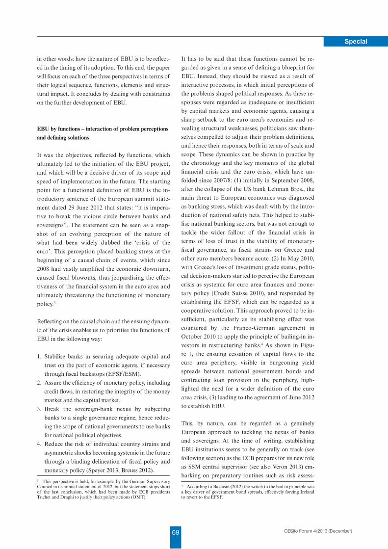
69 CESifo Forum 4/2013 (December)

Special

in other words: how the nature of EBU is to be reflect-

ed in the timing of its adoption. To this end, the paper

will focus on each of the three perspectives in terms of

their logical sequence, functions, elements and struc-

tural impact. It concludes by dealing with constraints

on the further development of EBU.

EBU by functions – interaction of problem perceptions and defining solutions

It was the objectives, reflected by functions, which

ultimately led to the initiation of the EBU project,

and which will be a decisive driver of its scope and

speed of implementation in the future. The starting

point for a functional definition of EBU is the in-

troductory sentence of the European summit state-

ment dated 29 June 2012 that states: “it is impera-

tive to break the vicious circle between banks and

sovereigns”. The statement can be seen as a snap-

shot of an evolving perception of the nature of

what had been widely dubbed the ‘crisis of the

euro’. This perception placed banking stress at the

beginning of a causal chain of events, which since

2008 had vastly amplified the economic downturn,

caused fiscal blowouts, thus jeopardising the effec-

tiveness of the financial system in the euro area and

ultimately threatening the functioning of monetary

policy.3

Reflecting on the causal chain and the ensuing dynam-

ic of the crisis enables us to prioritise the functions of

EBU in the following way:

1. Stabilise banks in securing adequate capital and

trust on the part of economic agents, if necessary

through fiscal backstops (EFSF/ESM).

2. Assure the efficiency of monetary policy, including

credit flows, in restoring the integrity of the money

market and the capital market.

3. Break the sovereign-bank nexus by subjecting

banks to a single governance regime, hence reduc-

ing the scope of national governments to use banks

for national political objectives.

4. Reduce the risk of individual country strains and

asymmetric shocks becoming systemic in the future

through a binding delineation of fiscal policy and

monetary policy (Speyer 2013; Breuss 2012).

3 This perspective is held, for example, by the German Supervisory Council in its annual statement of 2012, but the statement stops short of the last conclusion, which had been made by ECB presidents Trichet and Draghi to justify their policy actions (OMT).

It has to be said that these functions cannot be re-

garded as given in a sense of defining a blueprint for

EBU. Instead, they should be viewed as a result of

interactive processes, in which initial perceptions of

the problems shaped political responses. As these re-

sponses were regarded as inadequate or insufficient

by capital markets and economic agents, causing a

sharp setback to the euro area’s economies and re-

vealing structural weaknesses, politicians saw them-

selves compelled to adjust their problem definitions,

and hence their responses, both in terms of scale and

scope. These dynamics can be shown in practice by

the chronology and the key moments of the global

financial crisis and the euro crisis, which have un-

folded since 2007/8: (1) initially in September 2008,

after the collapse of the US bank Lehman Bros., the

main threat to Euro pean economies was diagnosed

as banking stress, which was dealt with by the intro-

duction of national safety nets. This helped to stabi-

lise national banking sectors, but was not enough to

tackle the wider fallout of the financial crisis in

terms of loss of trust in the viability of monetary-

fiscal governance, as fiscal strains on Greece and

other euro members became acute. (2) In May 2010,

with Greece’s loss of investment grade status, politi-

cal decision-makers started to perceive the European

crisis as systemic for euro area finances and mone-

tary policy (Credit Suisse 2010), and responded by

establishing the EFSF, which can be regarded as a

cooperative solution. This approach proved to be in-

sufficient, particularly as its stabilising effect was

countered by the Franco-German agreement in

October 2010 to apply the principle of bailing-in in-

vestors in restructuring banks.4 As shown in Figu-

re  1, the ensuing cessation of capital flows to the

euro area periphery, visible in burgeoning yield

spreads between national government bonds and

contracting loan provision in the periphery, high-

lighted the need for a wider definition of the euro

area crisis, (3) leading to the agreement of June 2012

to establish EBU.

This, by nature, can be regarded as a genuinely

European approach to tackling the nexus of banks

and sovereigns. At the time of writing, establishing

EBU institutions seems to be generally on track (see

following section) as the ECB prepares for its new role

as SSM central supervisor (see also Veron 2013) em-

barking on preparatory routines such as risk assess-

4 According to Bastasin (2012) the switch to the bail in principle was a key driver of government bond spreads, effectively forcing Ireland to revert to the EFSF.

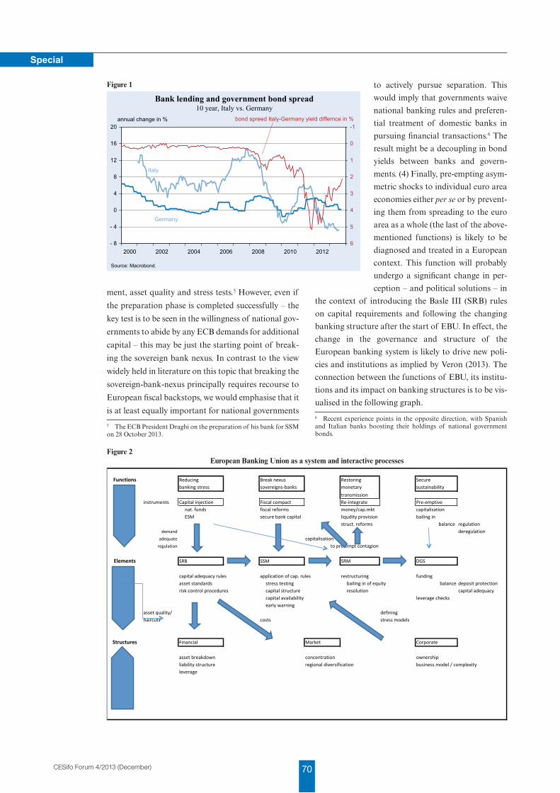
70CESifo Forum 4/2013 (December)

Special

ment, asset quality and stress tests.5 However, even if

the preparation phase is completed successfully – the

key test is to be seen in the willingness of national gov-

ernments to abide by any ECB demands for additional

capital – this may be just the starting point of break-

ing the sovereign bank nexus. In contrast to the view

widely held in literature on this topic that breaking the

sovereign-bank-nexus principally requires recourse to

European fiscal backstops, we would emphasise that it

is at least equally important for national governments

5 The ECB President Draghi on the preparation of his bank for SSM on 28 October 2013.

to actively pursue separation. This

would imply that governments waive

national banking rules and preferen-

tial treatment of domestic banks in

pursuing financial transactions.6 The

result might be a decoupling in bond

yields between banks and govern-

ments. (4) Finally, pre-empting asym-

metric shocks to individual euro area

economies either per se or by prevent-

ing them from spreading to the euro

area as a whole (the last of the above-

mentioned functions) is likely to be

diagnosed and treated in a European

context. This function will probably

undergo a significant change in per-

ception – and political solutions – in

the context of introducing the Basle  III (SRB) rules

on capital requirements and following the changing

banking structure after the start of EBU. In effect, the

change in the governance and structure of the

European banking system is likely to drive new poli-

cies and institutions as implied by Veron (2013). The

connection between the functions of EBU, its institu-

tions and its impact on banking structures is to be vis-

ualised in the following graph.

6 Recent experience points in the opposite direction, with Spanish and Italian banks boosting their holdings of national government bonds.

- 8

- 4

0

4

8

12

16

20

2000 2002 2004 2006 2008 2010 2012

-1

0

1

2

3

4

5

6

Bank lending and government bond spread10 year, Italy vs. Germany

Source: Macrobond.

Italy

Germany

annual change in % bond spreed Italy-Germany yield differnce in %

Figure 1

Figure 2European Banking Union as a system and interactive processes

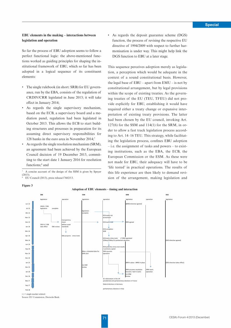
71 CESifo Forum 4/2013 (December)

Special

EBU elements in the making – interactions between legislation and operation

So far the process of EBU adoption seems to follow a

perfect functional logic: the above-mentioned func-

tions worked as guiding principles for shaping the in-

stitutional framework of EBU, which so far has been

adopted in a logical sequence of its constituent

elements:

• The single rulebook (in short: SRB) for EU govern-

ance, run by the EBA, consists of the regulation of

CRDIV/CRR legislated in June 2013; it will take

effect in January 2014;

• As regards the single supervisory mechanism,

based on the ECB, a supervisory board and a me-

diation panel, regulation had been legislated in

October 2013. This allows the ECB to start build-

ing structures and processes in preparation for its

assuming direct supervisory responsibilities for

128 banks in the euro area in November 2014;7

• As regards the single resolution mechanism (SRM),

an agreement had been achieved by the European

Council decision of 19 December 2013, commit-

ting to the start date 1 January 2016 for resolution

functions;8 and

7 A concise account of the design of the SSM is given by Speyer (2013).8 EU Council (2013), press release17602/13.

• As regards the deposit guarantee scheme (DGS)

function, the process of revising the respective EU

directive of 1994/2009 with respect to further har-

monisation is under way. This might help link the

DGS function to EBU at a later stage.

This sequence perceives adoption merely as legisla-

tion, a perception which would be adequate in the

context of a sound constitutional basis. However,

the legal base of EBU – apart from EMU – is not by

constitutional arrangement, but by legal provisions

within the scope of existing treaties. As the govern-

ing treaties of the EU (TEU, TFEU) did not pro-

vide explicitly for EBU, establishing it would have

required either a treaty change or expansive inter-

pretation of existing treaty provisions. The latter

had been chosen by the EU council, invoking Art.

127(6) for the SSM and 114(1) for the SRM, in or-

der to allow a fast track legislation process accord-

ing to Art. 14–16 TEU. This strategy, while facilitat-

ing the legislation process, confines EBU adoption

– i.e. the assignment of tasks and powers – to exist-

ing institutions, such as the EBA, the ECB, the

European Commission or the ESM. As these were

not made for EBU, their adequacy will have to be

‘life tested’ in practical operations. The results of

this life experience are then likely to demand revi-

sion of the arrangement, making legislation and

Figure 3Adoption of EBU elements – timing and interaction

( ) = single market related.

Source: EU Commission, Deutsche Bank.

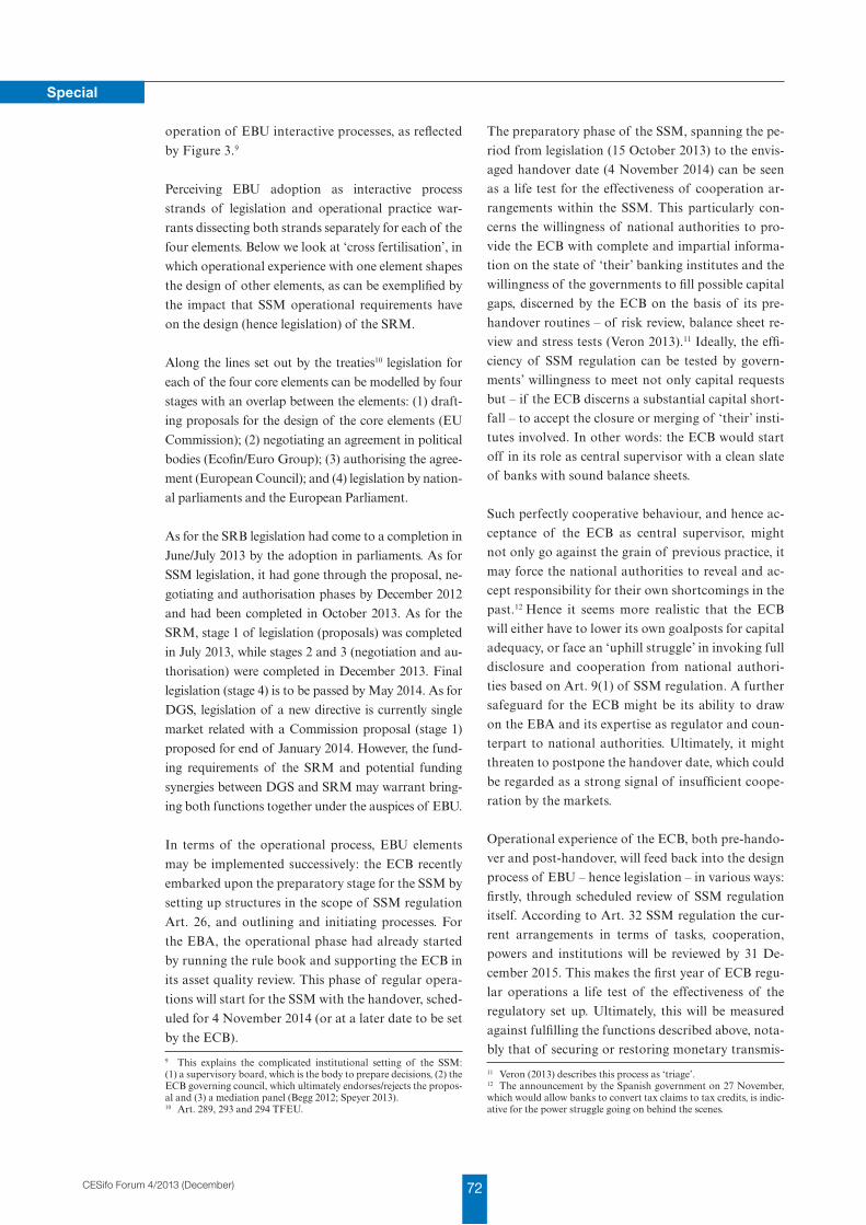
72CESifo Forum 4/2013 (December)

Special

operation of EBU interactive processes, as reflected

by Figure 3.9

Perceiving EBU adoption as interactive process

strands of legislation and operational practice war-

rants dissecting both strands separately for each of the

four elements. Below we look at ‘cross fertilisation’, in

which operational experience with one element shapes

the design of other elements, as can be exemplified by

the impact that SSM operational requirements have

on the design (hence legislation) of the SRM.

Along the lines set out by the treaties10 legislation for

each of the four core elements can be modelled by four

stages with an overlap between the elements: (1) draft-

ing proposals for the design of the core elements (EU

Commission); (2) negotiating an agreement in political

bodies (Ecofin/Euro Group); (3) authorising the agree-

ment (European Council); and (4) legislation by nation-

al parliaments and the Euro pean Parliament.

As for the SRB legislation had come to a completion in

June/July 2013 by the adoption in parliaments. As for

SSM legislation, it had gone through the proposal, ne-

gotiating and authorisation phases by December 2012

and had been completed in October 2013. As for the

SRM, stage 1 of legislation (proposals) was completed

in July 2013, while stages 2 and 3 (negotiation and au-

thorisation) were completed in December 2013. Final

legislation (stage 4) is to be passed by May 2014. As for

DGS, legislation of a new directive is currently single

market related with a Commission proposal (stage 1)

proposed for end of January 2014. However, the fund-

ing requirements of the SRM and potential funding

synergies between DGS and SRM may warrant bring-

ing both functions together under the auspices of EBU.

In terms of the operational process, EBU elements

may be implemented successively: the ECB recently

embarked upon the preparatory stage for the SSM by

setting up structures in the scope of SSM regulation

Art. 26, and outlining and initiating processes. For

the EBA, the operational phase had already started

by running the rule book and supporting the ECB in

its asset quality review. This phase of regular opera-

tions will start for the SSM with the handover, sched-

uled for 4 November 2014 (or at a later date to be set

by the ECB).

9 This explains the complicated institutional setting of the SSM: (1) a supervisory board, which is the body to prepare decisions, (2) the ECB governing council, which ultimately endorses/rejects the propos-al and (3) a mediation panel (Begg 2012; Speyer 2013).10 Art. 289, 293 and 294 TFEU.

The preparatory phase of the SSM, spanning the pe-

riod from legislation (15 October 2013) to the envis-

aged handover date (4 November 2014) can be seen

as a life test for the effectiveness of cooperation ar-

rangements within the SSM. This particularly con-

cerns the willingness of national authorities to pro-

vide the ECB with complete and impartial informa-

tion on the state of ‘their’ banking institutes and the

willingness of the governments to fill possible capital

gaps, discerned by the ECB on the basis of its pre-

handover routines – of risk review, balance sheet re-

view and stress tests (Veron 2013).11 Ideally, the effi-

ciency of SSM regulation can be tested by govern-

ments’ willingness to meet not only capital requests

but – if the ECB discerns a substantial capital short-

fall – to accept the closure or merging of ‘their’ insti-

tutes involved. In other words: the ECB would start

off in its role as central supervisor with a clean slate

of banks with sound balance sheets.

Such perfectly cooperative behaviour, and hence ac-

ceptance of the ECB as central supervisor, might

not only go against the grain of previous practice, it

may force the national authorities to reveal and ac-

cept responsibility for their own shortcomings in the

past.12 Hence it seems more realistic that the ECB

will either have to lower its own goalposts for capital

adequacy, or face an ‘uphill struggle’ in invoking full

disclosure and cooperation from national authori-

ties based on Art. 9(1) of SSM regulation. A further

safeguard for the ECB might be its ability to draw

on the EBA and its expertise as regulator and coun-

terpart to national authorities. Ultimately, it might

threaten to postpone the handover date, which could

be regarded as a strong signal of insufficient coope-

ration by the markets.

Operational experience of the ECB, both pre-hando-

ver and post-handover, will feed back into the design

process of EBU – hence legislation – in various ways:

firstly, through scheduled review of SSM regulation

itself. According to Art. 32 SSM regulation the cur-

rent arrangements in terms of tasks, cooperation,

powers and institutions will be reviewed by 31  De-

cember 2015. This makes the first year of ECB regu-

lar operations a life test of the effectiveness of the

regulatory set up. Ultimately, this will be measured

against fulfilling the functions described above, nota-

bly that of securing or restoring monetary transmis-

11 Veron (2013) describes this process as ‘triage’.12 The announcement by the Spanish government on 27 November, which would allow banks to convert tax claims to tax credits, is indic-ative for the power struggle going on behind the scenes.

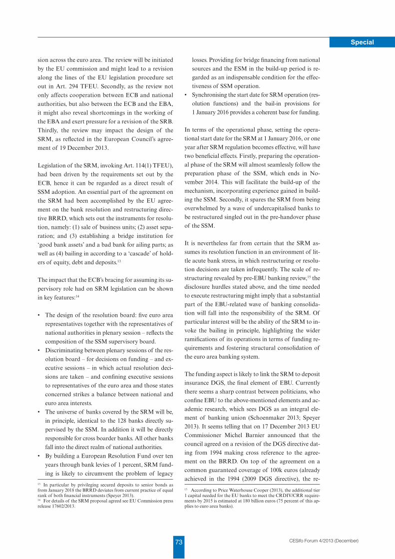
73 CESifo Forum 4/2013 (December)

Special

sion across the euro area. The review will be initiated

by the EU commission and might lead to a revision

along the lines of the EU legislation procedure set

out in Art. 294 TFEU. Secondly, as the review not

only affects cooperation between ECB and national

authorities, but also between the ECB and the EBA,

it might also reveal shortcomings in the working of

the EBA and exert pressure for a revision of the SRB.

Thirdly, the review may impact the design of the

SRM, as reflected in the European Council’s agree-

ment of 19 December 2013.

Legislation of the SRM, invoking Art. 114(1) TFEU),

had been driven by the requirements set out by the

ECB, hence it can be regarded as a direct result of

SSM adoption. An essential part of the agreement on

the SRM had been accomplished by the EU agree-

ment on the bank resolution and restructuring direc-

tive BRRD, which sets out the instruments for resolu-

tion, namely: (1) sale of business units; (2) asset sepa-

ration; and (3) establishing a bridge institution for

‘good bank assets’ and a bad bank for ailing parts; as

well as (4) bailing in according to a ‘cascade’ of hold-

ers of equity, debt and deposits.13

The impact that the ECB’s bracing for assuming its su-

pervisory role had on SRM legislation can be shown

in key features:14

• The design of the resolution board: five euro area

representatives together with the representatives of

national authorities in plenary session – reflects the

composition of the SSM supervisory board.

• Discriminating between plenary sessions of the res-

olution board – for decisions on funding – and ex-

ecutive sessions – in which actual resolution deci-

sions are taken – and confining executive sessions

to representatives of the euro area and those states

concerned strikes a balance between national and

euro area interests.

• The universe of banks covered by the SRM will be,

in principle, identical to the 128 banks directly su-

pervised by the SSM. In addition it will be directly

responsible for cross boarder banks. All other banks

fall into the direct realm of national authorities.

• By building a European Resolution Fund over ten

years through bank levies of 1 percent, SRM fund-

ing is likely to circumvent the problem of legacy

13 In particular by privileging secured deposits to senior bonds as from January 2018 the BRRD deviates from current practice of equal rank of both financial instruments (Speyer 2013). 14 For details of the SRM proposal agreed see EU Commission press release 17602/2013.

losses. Providing for bridge financing from national

sources and the ESM in the build-up period is re-

garded as an indispensable condition for the effec-

tiveness of SSM operation.

• Synchronising the start date for SRM operation (res-

olution functions) and the bail-in provisions for

1 January 2016 provides a coherent base for funding.

In terms of the operational phase, setting the opera-

tional start date for the SRM at 1 January 2016, or one

year after SRM regulation becomes effective, will have

two beneficial effects. Firstly, preparing the operation-

al phase of the SRM will almost seamlessly follow the

preparation phase of the SSM, which ends in No-

vember 2014. This will facilitate the build-up of the

mechanism, incorporating experience gained in build-

ing the SSM. Secondly, it spares the SRM from being

overwhelmed by a wave of undercapitalised banks to

be restructured singled out in the pre-handover phase

of the SSM.

It is nevertheless far from certain that the SRM as-

sumes its resolution function in an environment of lit-

tle acute bank stress, in which restructuring or resolu-

tion decisions are taken infrequently. The scale of re-

structuring revealed by pre-EBU banking review,15 the

disclosure hurdles stated above, and the time needed

to execute restructuring might imply that a substantial

part of the EBU-related wave of banking consolida-

tion will fall into the responsibility of the SRM. Of

particular interest will be the ability of the SRM to in-

voke the bailing in principle, highlighting the wider

ramifications of its operations in terms of funding re-

quirements and fostering structural consolidation of

the euro area banking system.

The funding aspect is likely to link the SRM to deposit

insurance DGS, the final element of EBU. Currently

there seems a sharp contrast between politicians, who

confine EBU to the above-mentioned elements and ac-

ademic research, which sees DGS as an integral ele-

ment of banking union (Schoenmaker 2013; Speyer

2013). It seems telling that on 17 December 2013 EU

Commissioner Michel Barnier announced that the

council agreed on a revision of the DGS directive dat-

ing from 1994 making cross reference to the agree-

ment on the BRRD. On top of the agreement on a

common guaranteed coverage of 100k euros (already

achieved in the 1994 (2009 DGS directive), the re-

15 According to Price Waterhouse Cooper (2013), the additional tier 1 capital needed for the EU banks to meet the CRDIV/CRR require-ments by 2015 is estimated at 180 billion euros (75 percent of this ap-plies to euro area banks).

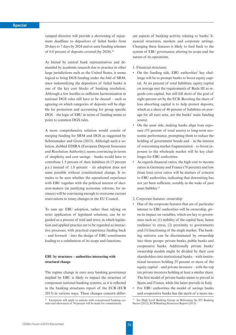
74CESifo Forum 4/2013 (December)

Special

vamped directive will provide a shortening of repay-

ment deadlines to depositors of failed banks from

20 days to 7 days by 2024 and ex-ante funding schemes

of 0.8 percent of deposits covered (by 2024).16

As hinted by central bank representatives and de-

manded by academic research due to practice in other

large jurisdictions such as the United States, it seems

logical to bring DGS funding under the fold of SRM,

since indemnifying the depositors of failed banks is

one of the key cost blocks of banking resolution.

Although a few hurdles to sufficient harmonisation in

national DGS rules still have to be cleared – such as

agreeing on which categories of deposits will be eligi-

ble for protection and accounting for group specific

DGS – the logic of EBU in terms of funding seems to

point to common DGS rules.

A more comprehensive solution would consist of

merging funding for SRM and DGS as suggested by

Schoenmaker and Gross (2013). Although such a so-

lution, dubbed EDIRA (European Deposit Insurance

and Resolution Authority), seems convincing in terms

of simplicity and cost savings – banks would have to

contribute 1.5 percent of their liabilities (0.15 percent

p.a.) instead of 1.8 percent – its adoption does not

seem possible without constitutional change. It re-

mains to be seen whether the operational experience

with EBU together with the political interest of deci-

sion-makers (in justifying economic reforms, for in-

stance) will be convincing enough to overcome current

reservations to treaty changes in the EU Council.

To sum up: EBU adoption, rather than relying on

strict application of legislated solutions, can be re-

garded as a process of trial and error, in which legisla-

tion and applied practice are to be regarded as interac-

tive processes, with practical experience feeding back

– and forward – into the design of EBU constituents

leading to a redefinition of its scope and functions.

EBU by structures – authorities interacting with structural change

The regime change in euro area banking governance

implied by EBU is likely to impact the structure of

component national banking systems, as it is reflected

in the banking structures report of the ECB (ECB

2013) in various ways. These changes concern differ-

16 Exceptions will apply to nations with concentrated banking sys-tems and allowances of 30 percent will be made for commitments

ent aspects of banking activity relating to banks’ fi-

nancial structures, markets and corporate settings.

Changing these features is likely to feed back to the

system of EBU governance, altering its scope and the

nature of its operations.

1. Financial structures

• On the funding side, EBU authorities’ key chal-

lenge will be to prompt banks to boost equity capi-

tal. At six percent of total liabilities, equity capital

on average met the requirements of Basle III as re-

gards core capital, but still fell short of the goal of

eight percent set by the ECB. Boosting the share of

loss absorbing capital is to help protect deposits,

which at a share of 46 percent of liabilities on aver-

age for all euro area, are the banks’ main funding

source.

• On the asset side, making banks align loan expo-

sure (55 percent of total assets) to long-term eco-

nomic performance, prompting them to reduce the

holding of government bonds and – in the interest

of overcoming market fragmentation – to boost ex-

posure to the wholesale market will be key chal-

lenges for EBU authorities.

• As regards financial ratios, the high cost to income

ratios in Germany and France (70 percent) and low

(loan loss) cover ratios will be matters of concern

to EBU authorities, indicating that downsizing has

not yet been sufficient, notably in the wake of past

asset bubbles.17

2. Corporate features: ownership

• One of the corporate features that are of particular

interest to EBU authorities will be ownership, giv-

en its impact on variables, which are key to govern-

ance such as: (1) stability of the capital base, hence

resilience to stress, (2) proximity to governments

and (3) functioning of the single market. The bank-

ing universe can be discriminated by ownership

into three groups: private banks, public banks and

cooperative banks. Addition ally private banks’

ownership models might be divided by their core

shareholders into institutional banks – with institu-

tional investors holding 25 percent or more of the

equity capital – and private investors – with the top

ten private investors holding at least a similar share.

The first model of private banks seems to prevail in

Spain and France, while the latter prevails in Italy.

• For EBU authorities the model of savings banks

and cooperative banks has the merit of a more sta-

17 See High Level Banking Group on Reforming the EU Banking Sector (2012); ECB Banking Structures Report (2013).

75 CESifo Forum 4/2013 (December)

Special

ble investor base, but seems prone to government

influence – at least in the case of public banks. The

model of a stable investor base, prevalent in

Germany, has been vindicated in the last two reces-

sions, as it had been savings banks and cooperative

banks, whose lending helped avoid a credit crunch,

whereas it is the notion of often observed proximi-

ty to local governments, which might reflect nega-

tively on breaking the bank sovereign nexus.

• As regards the model of private banks – in particu-

lar those with core holdings of institutional inves-

tors – it is investors’ demand for returns that might

drive performance, but also the higher risk-taking

of these institutes. Hence in terms of EBU func-

tions, for the EBU authorities both models seem to

have their merits, even in an environment of accel-

erating structural adjustment in terms of downsiz-

ing, deleveraging and market concentration.

3. Market features

The structural diversity of national banking markets

in terms of size, concentration and international expo-

sure is to pose a key challenge to EBU authorities,

which can be exemplified as follows:

• Accommodating the downsizing of offshore cen-

tres like Ireland, Luxemburg and Malta in the wake

of the eroding prospects of regulatory arbitrage,18

• Gauging risk and cover ratios for network banking

systems like German savings banks or French co-

operative banks, which are comparable to branch

institutes,19

• Meeting the conflicting demands of cross border

banks (like Deutsche Bank and BNP Paribas) and

regional institutes (like German and Spanish sav-

ings banks). Not privileging one group – as might

be possible by different practices of national super-

visors and the ECB – while at the same time not

obviating EBU related tendencies for concentra-

tion might imply a dilemma for EBU authorities.

Legislation in pursuit of the further development of EBU

Even after the handover of governance to EBU insti-

tutions, the institutional architecture of EBU will be

provisional (see also Veron 2013). This regards the or-

18 These can be discerned by bank balance sheet to GDP ratios of up to 1,000 percent in contrast to 350 percent for the euro area average.19 Germany with a market share of 30 percent for the largest five and just 20 branches vs. 120 in Spain reflects the prevalence of public banks. The GCEE (2013) makes the risk of banking groups a major focus in its annual report.

ganisational arrangement within the institutions –

such as the distribution of powers between national

supervisors and the ECB within the SSM – as well as

the choice of the institutions as such, their scope and

their powers. Establishing a permanent arrangement

regarding restructuring/resolution and bringing the

DGS function into the fold of EBU will involve fur-

ther practical challenges.

There is a cascade of legal options available in pursuit

of a more permanent EBU arrangement:

1. The first option is the scheduled review of the insti-

tutional arrangement within the SSM according to

Art. 32 SSM regulation by 31 December 2015 and

every three years thereafter. This review will follow

the standard procedure of Art. 294 TFEU with the

Commission initiating the process and the Council

and Parliament completing legislation. A similar

arrangement might be expected as regards the

SRM. Experience of this process will indicate the

chances of pursuing more profound legal changes

along the other two options.

2. The next option would be a change in the institu-

tional setting for EBU, notably establishing a sepa-

rate SRM authority and a European DGS author-

ity including fund(s) for these two elements. To this

end, a change in the treaties, or more specifically

the TFEU, seems warranted. Such a change could

happen by a so-called ‘simplified revision proce-

dure’ according to Art. 48(6). This demands ap-

proval by member states according to their consti-

tutional requirements – usually by national parlia-

ments, in some states by referendums.20 Even the

simplified revision procedure, while acceptable to

euro area governments, may face major political re-

sistance from countries not participating in the

euro (outs) as seen in the event of the fiscal com-

pact, whose adoption as EU law was prevented by

Britain’s veto. Given the sensitivity of the Britain to

financial issues, a veto by the Britain seems a dis-

tinct risk –particularly in the run-up to the 2017

referendum.

3. The ultimate and most encompassing change

would concern the scope of EBU in the context of

monetary, fiscal and political union. Linking the

EBU to such a wider context, making banking pol-

icy an exclusive competence of the EU would re-

quire the ‘ordinary revision procedure’ of Art. 48(2)

20 Such an undertaking is occasionally compared to legislating the ESM in February 2012, or the so-called fiscal compact in March 2012, but was seen as too intrusive to be pursued in the standard legislation procedure as was the case with the ESM – see also Veron (2013).

76CESifo Forum 4/2013 (December)

Special

to 48(5). This would, in turn, usually call for a

European convention, assembling representatives

of national parliaments and the European parlia-

ment, national governments and the EU commis-

sion. However, this option, although pursued by

the German government, seems to be meeting with

little support against a backdrop of strong Euro-

sceptic undercurrents across the euro area coun-

tries. Hence it does not seem available at least until

early 2018, after the EU referendum in Britain and

national elections in the three largest EU econo-

mies. These events may bring significant changes to

the political landscape by either unveiling new op-

tions or calling past achievements into question.

References

Begg, I. (2012), “Banking Union: Inevitable, But Profoundly Challenging”, CESifo Forum 13(4), 15–20.

Bastasin, C. (2012), Saving Europe – How National Politics Nearly Destroyed the Euro, Washington DC: Brookings Press.

Breuss, F. (2012), “European Banking Union: Necessary But Not Enough to Fix the Euro Crisis”, CESifo Forum 13(4), 28–32.

Credit Suisse Fixed Income Research (2010), Fixed Income Strategy, London.

Credit Suisse Fixed Income Research (2011), EFSF (R)evolution, 16 August, London.

European Union, (2013a), European Council Regulation on Single Supervisory Mechanism, Reg. (EU) 1024/2013.

European Central Bank (2013b), ECB Starts Comprehensive Assessment in Advance of Supervisory Role, Press note of 23 October, Frankfurt.

European Central Bank (2013c), Banking Structures Report, Novem-ber, Frankfurt.

European Union, (2010a), Regulation (EU) 407/2010 on European Financial Stabilisation Mechanism, June, Brussels.

European Union, (2010b), Regulation (EU) 1092/2010 on European Systemic Risk Board, Brussels.

German Council of Economic Experts (GCEE, 2013), Germany Heading for European Banking Union, Annual Report 2013/14, Wiesbaden.

Goyal, R. et al. (2013), A Banking Union for the Euro Area, IMF Staff Discussion Notes 13/1.

High-level Expert Group on Reforming the Structure of the EU Banking Sector (2012), Final Report, 2 October, Brussels.

Lautenschläger, S. (2013), “Stresstest soll streng ausfallen”, Interview with German Daily Handelsblatt, 25 November, Frankfurt.

Mersch, Y. (2013), The European Banking Union – First Steps on a Long March, Speech on Finanzplatztag, 27 February, Frankfurt.

Price Waterhouse Cooper (2013), De-leverage Take 2: Making a Virtue of Necessity, PWC publication, 28 November, London.

Schneider, C. (2013), “Einführung und politische Schlussfolgerungen, Bankenunion – wer zahlt die Zeche”, WISO Diskurs, June, Berlin: Friedrich Ebert Stiftung, 4–7.

Schoenmaker, D. and D. Gross (2013), A European Deposit Insurance and Resolution Fund – An Update, Duisenberg School of Finance, Amsterdam.

Speyer, B. (2012), EU Banking Union – Do It Right, Not Hastily, EU Monitor, DB Research, July, Frankfurt.

Speyer, B. (2013), EU Banking Union – Right Idea, Poor Execution, EU Monitor, DB Research, 4 September, Frankfurt.

Veron, N. (2013), “A Realistic Bridge towards European Banking Union”, Bruegel Policy Contribution 2013/09.

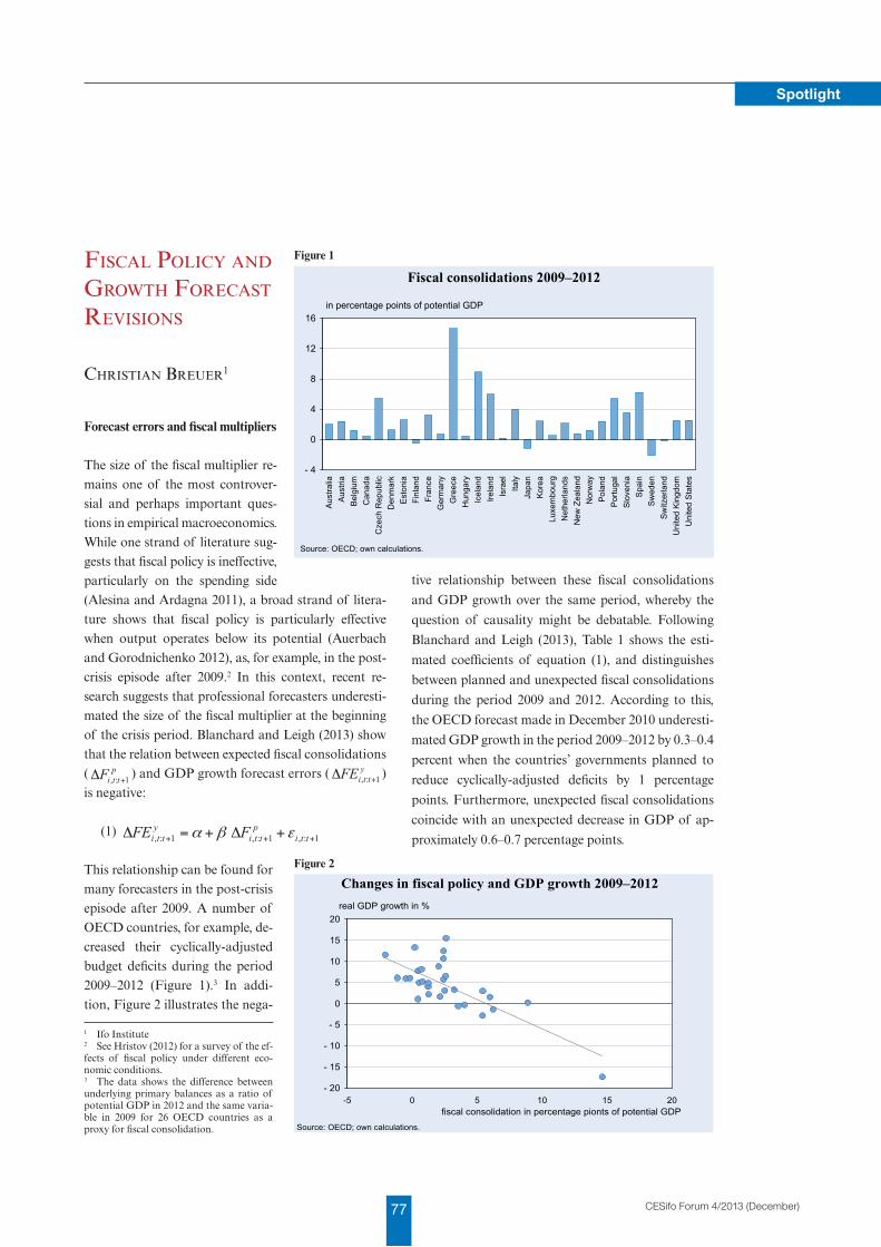
77 CESifo Forum 4/2013 (December)

Spotlight

Fiscal Policy and Growth Forecast revisions

christian Breuer1

Forecast errors and fiscal multipliers

The size of the fiscal multiplier re-mains one of the most controver-sial and perhaps important ques-tions in empirical macroeconomics. While one strand of literature sug-gests that fiscal policy is ineffective, particularly on the spending side (Alesina and Ardagna 2011), a broad strand of litera-ture shows that fiscal policy is particularly effective when output operates below its potential (Auerbach and Gorodnichenko 2012), as, for example, in the post-crisis episode after 2009.2 In this context, recent re-search suggests that professional forecasters underesti-mated the size of the fiscal multiplier at the beginning of the crisis period. Blanchard and Leigh (2013) show that the relation between expected fiscal consolidations ( p

ttiF 1:, +Δ  ) and GDP growth forecast errors ( yttiFE 1:, +Δ  )

is negative:

(1)  

1:,1:,1:, +++ +Δ+=Δ ttiptti

ytti FFE εβα  

This relationship can be found for many forecasters in the post-crisis episode after 2009. A number of OECD countries, for example, de-creased their cyclically-adjusted budget deficits during the period 2009–2012 (Figure 1).3 In addi-tion, Figure 2 illustrates the nega-

1 Ifo Institute2 See Hristov (2012) for a survey of the ef-fects of fiscal policy under different eco-nomic conditions.3 The data shows the difference between underlying primary balances as a ratio of potential GDP in 2012 and the same varia-ble in 2009 for 26 OECD countries as a proxy for fiscal consolidation.

tive relationship between these fiscal consolidations

and GDP growth over the same period, whereby the

question of causality might be debatable. Following

Blanchard and Leigh (2013), Table 1 shows the esti-

mated coefficients of equation (1), and distinguishes

between planned and unexpected fiscal consolidations

during the period 2009 and 2012. According to this,

the OECD forecast made in December 2010 underesti-

mated GDP growth in the period 2009–2012 by 0.3–0.4

percent when the countries’ governments planned to

reduce cyclically-adjusted deficits by 1 percentage

points. Furthermore, unexpected fiscal consolidations

coincide with an unexpected decrease in GDP of ap-

proximately 0.6–0.7 percentage points.

- 4

0

4

8

12

16A

ustra

liaA

ustri

aB

elgi

umC

anad

aC

zech

Rep

ublic

Den

mar

kE

ston

iaFi

nlan

dFr

ance

Ger

man

yG

reec

eH

unga

ryIc

elan

dIre

land

Isra

elIta

lyJa

pan

Kor

eaLu

xem

bour

gN

ethe

rland

sN

ew Z

eala

ndN

orw

ayP

olan

dP

ortu

gal

Slo

veni

aS

pain

Sw

eden

Sw

itzer

land

Uni

ted

Kin

gdom

Uni

ted

Sta

tes

Fiscal consolidations 2009–2012

in percentage points of potential GDP

Source: OECD; own calculations.

Figure 1

- 20

- 15

- 10

- 5

0

5

10

15

20

-5 0 5 10 15 20

Changes in fiscal policy and GDP growth 2009–2012real GDP growth in %

Source: OECD; own calculations.

fiscal consolidation in percentage pionts of potential GDP

Figure 2

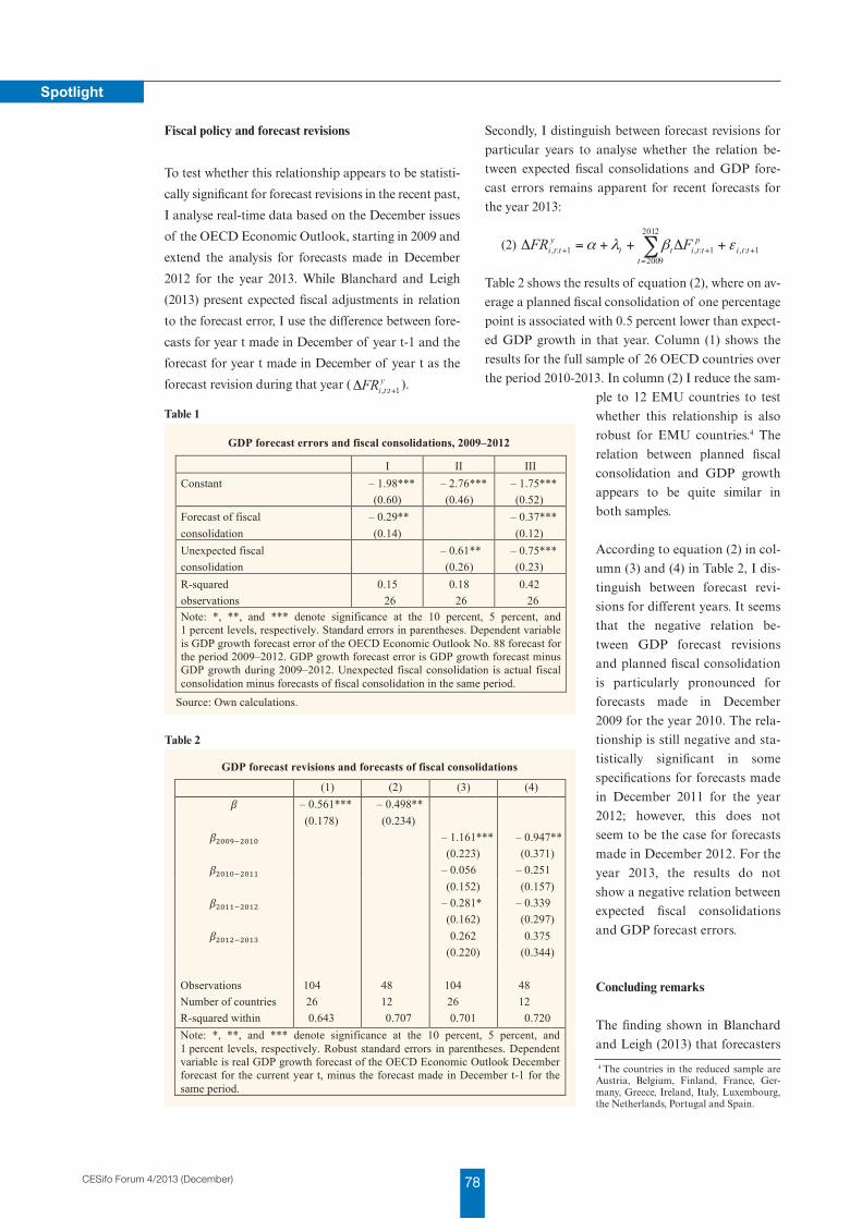
78CESifo Forum 4/2013 (December)

Spotlight

Fiscal policy and forecast revisions

To test whether this relationship appears to be statisti-

cally significant for forecast revisions in the recent past,

I analyse real-time data based on the December issues

of the OECD Economic Outlook, starting in 2009 and

extend the analysis for forecasts made in December

2012 for the year 2013. While Blanchard and Leigh

(2013) present expected fiscal adjustments in relation

to the forecast error, I use the difference between fore-

casts for year t made in December of year t-1 and the

forecast for year t made in December of year t as the

forecast revision during that year ( yttiFR 1:, +Δ  ).

Secondly, I distinguish between forecast revisions for

particular years to analyse whether the relation be-

tween expected fiscal consolidations and GDP fore-

cast errors remains apparent for recent forecasts for

the year 2013:

(2)

 

1:,

2012

20091:,1:, +

=++ +Δ++=Δ ∑ tti

t

pttitt

ytti FFR εβλα  

Table 2 shows the results of equation (2), where on av-

erage a planned fiscal consolidation of one percentage

point is associated with 0.5 percent lower than expect-

ed GDP growth in that year. Column (1) shows the

results for the full sample of 26 OECD countries over

the period 2010-2013. In column (2) I reduce the sam-

ple to 12 EMU countries to test

whether this relationship is also

robust for EMU countries.4 The

relation between planned fiscal

consolidation and GDP growth

appears to be quite similar in

both samples.

According to equation (2) in col-

umn (3) and (4) in Table 2, I dis-

tinguish between forecast revi-

sions for different years. It seems

that the negative relation be-

tween GDP forecast revisions

and planned fiscal consolidation

is particularly pronounced for

forecasts made in December

2009 for the year 2010. The rela-

tionship is still negative and sta-

tistically significant in some

specifications for forecasts made

in December 2011 for the year

2012; however, this does not

seem to be the case for forecasts

made in December 2012. For the

year 2013, the results do not

show a negative relation between

expected fiscal consolidations

and GDP forecast errors.

Concluding remarks

The finding shown in Blanchard

and Leigh (2013) that forecasters

4 The countries in the reduced sample are Austria, Belgium, Finland, France, Ger-many, Greece, Ireland, Italy, Luxembourg, the Netherlands, Portugal and Spain.

Table 1

GDP forecast errors and fiscal consolidations, 2009–2012

I II III

Constant – 1.98 *** – 2.76 *** – 1.75 ***

(0.60 ) (0.46 ) (0.52 )

Forecast of fiscal – 0.29 ** – 0.37 ***

consolidation (0.14 ) (0.12 )

Unexpected fiscal

– 0.61 ** – 0.75 *** consolidation

(0.26 ) (0.23 )

R-squared 0.15 0.18 0.42 observations 26 26 26 Note: *, **, and *** denote significance at the 10 percent, 5 percent, and 1 percent levels, respectively. Standard errors in parentheses. Dependent variable is GDP growth forecast error of the OECD Economic Outlook No. 88 forecast for the period 2009–2012. GDP growth forecast error is GDP growth forecast minus GDP growth during 2009–2012. Unexpected fiscal consolidation is actual fiscal consolidation minus forecasts of fiscal consolidation in the same period.

Source: Own calculations.  

Table 1

Table 2

GDP forecast revisions and forecasts of fiscal consolidations

(1) (2) (3) (4) ! – 0.561 *** – 0.498 **

(0.178 ) (0.234 ) !!""#!!"#" – 1.161 *** – 0.947 **

(0.223 ) (0.371 ) !!"#"!!"## – 0.056 – 0.251

(0.152 ) (0.157 ) !!"##!!"#! – 0.281 * – 0.339

(0.162 ) (0.297 ) !!"#!!!"#$ 0.262 0.375

(0.220 ) (0.344 ) Observations 104 48 104 48 Number of countries 26 12 26 12 R-squared within 0.643 0.707 0.701 0.720 Note: *, **, and *** denote significance at the 10 percent, 5 percent, and 1 percent levels, respectively. Robust standard errors in parentheses. Dependent variable is real GDP growth forecast of the OECD Economic Outlook December forecast for the current year t, minus the forecast made in December t-1 for the same period.

Table 2

79 CESifo Forum 4/2013 (December)

Spotlight

underestimated the size of the fiscal multiplier has been extensively debated in the recent past. While this relationship seems to be particularly pronounced for the first year following the economic crisis in 2009, new data for the year 2013 suggest that expected fiscal consolidations do not influence the quality of recent forecasts made by the OECD. A number of potential factors might explain why recent forecasts appear to be more efficient, as compared to forecasts for the year 2010. It is conceivable that forecasts made in 2009 hardly anticipated the macroeconomic effects of the so-called euro crisis after 2009, even although the new debate on the size of the fiscal multiplier may also have helped to improve forecasting efficiency.

References

Alesina, A. and S. Ardagna (2011), “Large Changes in Fiscal Policy: Taxes vs. Spending”, in: Brown, J. R. (ed.), Tax Policy and the Economy 24, Chicago: University of Chicago Press, 35-68.

Auerbach, A. and Y. Gorodnichenko (2013), Fiscal Multipliers in Recession and Expansion, NBER Working Paper 17447.

Blanchard, O. and D. Leigh (2013), “Growth Forecast Errors and Fiscal Multipliers”, American Economic Review 103, 117-120.

Hristov, A. (2012), The Effects of Discretionary Fiscal Stimulus: A Survey, MPRA Paper 44714.

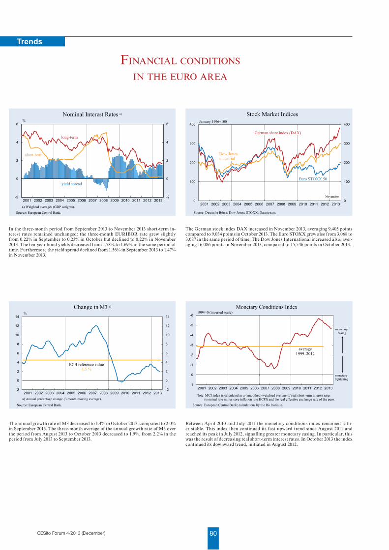
80CESifo Forum 4/2013 (December)

Trends

Financial conditions

in the euro area

The annual growth rate of M3 decreased to 1.4% in October 2013, compared to 2.0% in September 2013. The three-month average of the annual growth rate of M3 over the period from August 2013 to October 2013 decreased to 1.9%, from 2.2% in the period from July 2013 to September 2013.

Between April 2010 and July 2011 the monetary conditions index remained rath-er stable. This index then continued its fast upward trend since August 2011 and reached its peak in July 2012, signalling greater monetary easing. In particular, this was the result of decreasing real short-term interest rates. In October 2013 the index continued its downward trend, initiated in August 2012.

In the three-month period from September 2013 to November 2013 short-term in-terest rates remained unchanged: the three-month EURIBOR rate grew slightly from 0.22% in September to 0.23% in October but declined to 0.22% in November 2013. The ten-year bond yields decreased from 1.78% to 1.69% in the same period of time. Furthermore the yield spread declined from 1.56% in September 2013 to 1.47% in November 2013.

The German stock index DAX increased in November 2013, averaging 9,405 points compared to 9,034 points in October 2013. The Euro STOXX grew also from 3,068 to 3,087 in the same period of time. The Dow Jones International increased also, aver-aging 16,086 points in November 2013, compared to 15,546 points in October 2013.

-2

0

2

4

6

2001 2002 2003 2004 2005 2006 2007 2008 2009 2010 2011 2012 2013-2

0

2

4

6%

Nominal Interest Rates a)

long-term

a) Weighted averages (GDP weights).

Source: European Central Bank.

yield spread

short-term

0

100

200

300

400

2001 2002 2003 2004 2005 2006 2007 2008 2009 2010 2011 2012 20130

100

200

300

400

Stock Market IndicesJanuary 1996=100

Source: Deutsche Börse; Dow Jones; STOXX; Datastream.

November

Euro STOXX 50

Dow Jones industrial

German share index (DAX)

-2

0

2

4

6

8

10

12

14

2001 2002 2003 2004 2005 2006 2007 2008 2009 2010 2011 2012 2013-2

0

2

4

6

8

10

12

14%

Change in M3 a)

a) Annual percentage change (3-month moving average).

Source: European Central Bank.

ECB reference value4.5 %

2001 2002 2003 2004 2005 2006 2007 2008 2009 2010 2011 2012 2013

-6

-5

-4

-3

-2

-1

0

1

1994=0 (inverted scale)Monetary Conditions Index

Source: European Central Bank; calculations by the Ifo Institute.

average1999–2012

monetaryeasing

monetarytightening

Note: MCI index is calculated as a (smoothed) weighted average of real short-term interest rates (nominal rate minus core inflation rate HCPI) and the real effective exchange rate of the euro.

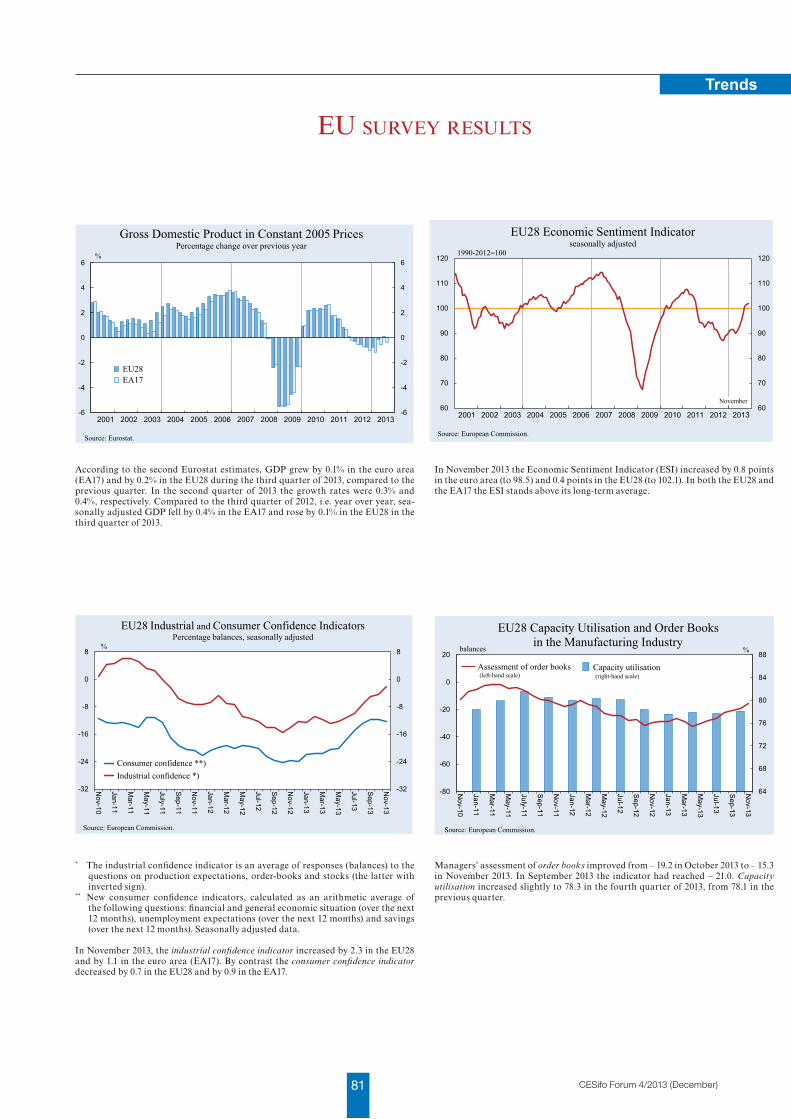
81 CESifo Forum 4/2013 (December)

Trends

eu survey results

* The industrial confidence indicator is an average of responses (balances) to the questions on production expectations, order-books and stocks (the latter with inverted sign).

** New consumer confidence indicators, calculated as an arithmetic average of the following questions: financial and general economic situation (over the next 12 months), unemployment expectations (over the next 12 months) and savings (over the next 12 months). Seasonally adjusted data.

In November 2013, the industrial confidence indicator increased by 2.3 in the EU28 and by 1.1 in the euro area (EA17). By contrast the consumer confidence indicator decreased by 0.7 in the EU28 and by 0.9 in the EA17.

Managers’ assessment of order books improved from – 19.2 in October 2013 to – 15.3 in November 2013. In September 2013 the indicator had reached – 21.0. Capacity utilisation increased slightly to 78.3 in the fourth quarter of 2013, from 78.1 in the previous quarter.

According to the second Eurostat estimates, GDP grew by 0.1% in the euro area (EA17) and by 0.2% in the EU28 during the third quarter of 2013, compared to the previous quarter. In the second quarter of 2013 the growth rates were 0.3% and 0.4%, respectively. Compared to the third quarter of 2012, i.e. year over year, sea-sonally adjusted GDP fell by 0.4% in the EA17 and rose by 0.1% in the EU28 in the third quarter of 2013.

In November 2013 the Economic Sentiment Indicator (ESI) increased by 0.8 points in the euro area (to 98.5) and 0.4 points in the EU28 (to 102.1). In both the EU28 and the EA17 the ESI stands above its long-term average.

-6

-4

-2

0

2

4

6

2001 2002 2003 2004 2005 2006 2007 2008 2009 2010 2011 2012 2013-6

-4

-2

0

2

4

6%

EU28 EA17

Gross Domestic Product in Constant 2005 PricesPercentage change over previous year

Source: Eurostat.

60

70

80

90

100

110

120

2001 2002 2003 2004 2005 2006 2007 2008 2009 2010 2011 2012 201360

70

80

90

100

110

120

EU28 Economic Sentiment Indicatorseasonally adjusted

November

Source: European Commission.

1990-2012=100

-32

-24

-16

-8

0

8

Nov-10

Jan-11

Mar-11

May-11

July-11

Sep-11

Nov-11

Jan-12

Mar-12

May-12

Jul-12

Sep-12

Nov-12

Jan-13

Mar-13

May-13

Jul-13

Sep-13

Nov-13

-32

-24

-16

-8

0

8

Consumer confidence **) Industrial confidence *)

EU28 Industrial and Consumer Confidence IndicatorsPercentage balances, seasonally adjusted

%

Source: European Commission.

64

68

72

76

80

84

88

-80

-60

-40

-20

0

20

Nov-10

Jan-11

Mar-11

May-11

July-11

Sep-11

Nov-11

Jan-12

Mar-12

May-12

Jul-12

Sep-12

Nov-12

Jan-13

Mar-13

May-13

Jul-13

Sep-13

Nov-13

%balances

EU28 Capacity Utilisation and Order Booksin the Manufacturing Industry

Source: European Commission.

(left-hand scale)Assessment of order books

(right-hand scale)Capacity utilisation

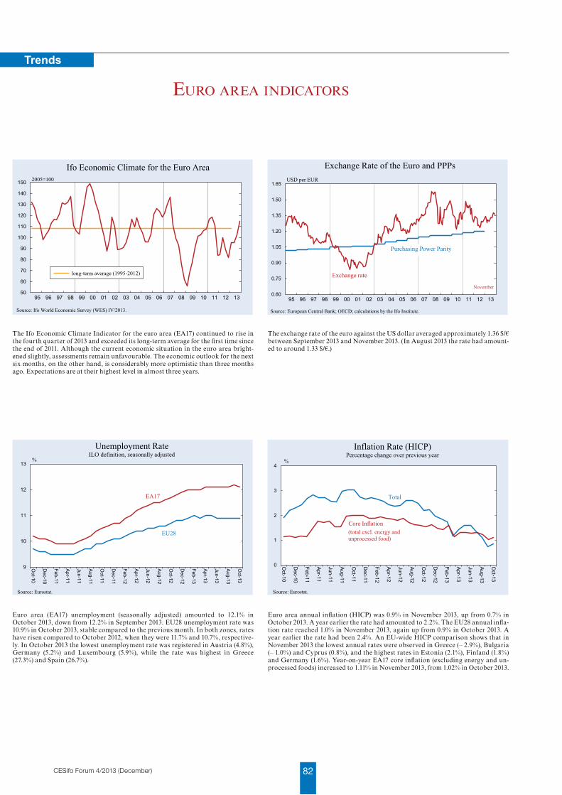
82CESifo Forum 4/2013 (December)

Trends

euro area indicators

Euro area (EA17) unemployment (seasonally adjusted) amounted to 12.1% in October 2013, down from 12.2% in September 2013. EU28 unemployment rate was 10.9% in October 2013, stable compared to the previous month. In both zones, rates have risen compared to October 2012, when they were 11.7% and 10.7%, respective-ly. In October 2013 the lowest unemployment rate was registered in Austria (4.8%), Germany (5.2%) and Luxembourg (5.9%), while the rate was highest in Greece (27.3%) and Spain (26.7%).

Euro area annual inflation (HICP) was 0.9% in November 2013, up from 0.7% in October 2013. A year earlier the rate had amounted to 2.2%. The EU28 annual infla-tion rate reached 1.0% in November 2013, again up from 0.9% in October 2013. A year earlier the rate had been 2.4%. An EU-wide HICP comparison shows that in November 2013 the lowest annual rates were observed in Greece (– 2.9%), Bulgaria (– 1.0%) and Cyprus (0.8%), and the highest rates in Estonia (2.1%), Finland (1.8%) and Germany (1.6%). Year-on-year EA17 core inflation (excluding energy and un-processed foods) increased to 1.11% in November 2013, from 1.02% in October 2013.

The Ifo Economic Climate Indicator for the euro area (EA17) continued to rise in the fourth quarter of 2013 and exceeded its long-term average for the first time since the end of 2011. Although the current economic situation in the euro area bright-ened slightly, assessments remain unfavourable. The economic outlook for the next six months, on the other hand, is considerably more optimistic than three months ago. Expectations are at their highest level in almost three years.

The exchange rate of the euro against the US dollar averaged approximately 1.36 $/€ between September 2013 and November 2013. (In August 2013 the rate had amount-ed to around 1.33 $/€.)

0

1

2

3

4

Oct-10

Dec-10

Feb-11

Apr-11

Jun-11

Aug-11

Oct-11

Dec-11

Feb-12

Apr-12

Jun-12

Aug-12

Oct-12

Dec-12

Feb-13

Apr-13

Jun-13

Aug-13

Oct-13

Inflation Rate (HICP)Percentage change over previous year

Core Inflation (total excl. energy and unprocessed food)

Total

%

Source: Eurostat.

9

10

11

12

13

Oct-10

Dec-10

Feb-11

Apr-11

Jun-11

Aug-11

Oct-11

Dec-11

Feb-12

Apr-12

Jun-12

Aug-12

Oct-12

Dec-12

Feb-13

Apr-13

Jun-13

Aug-13

Oct-13

Unemployment RateILO definition, seasonally adjusted

%

Source: Eurostat.

EU28

EA17

95 96 97 98 99 00 01 02 03 04 05 06 07 08 09 10 11 12 130.60

0.75

0.90

1.05

1.20

1.35

1.50

1.65

Exchange Rate of the Euro and PPPs

Source: European Central Bank; OECD; calculations by the Ifo Institute.

Exchange rate

Purchasing Power Parity

USD per EUR

November

95 96 97 98 99 00 01 02 03 04 05 06 07 08 09 10 11 12 1350

60

70

80

90

100

110

120

130

140

150

Ifo Economic Climate for the Euro Area2005=100

Source: Ifo World Economic Survey (WES) IV/2013.

long-term average (1995-2012)

Vo l u m e 11, No. 4 W i N t e r 2 013

Research Report

Reform Model

Database

News

Forum

Interest Groups and Bank reGulatIon

Florian Buck

Charles W. Calomiris and Stephen H. Haber

James R. Barth, Apanard Penny Prabha and Wenling Lu

Kay Shimizu and Kenji E. Kushida

Jenny Simon

Nadine Fabritz andOliver Falck

the role of Imperfect fInancIal markets for socIal redIstrIButIon

local dereGulatIon of the Wholesale BroadBand access market

suBnatIonal Government system reforms

rIsk of poverty and socIal exclusIon WorldWIde BIke sharInG proGrammes

Influence of ImmIGrant arrIval aGe

neW at dIce dataBase, conferences, Books

CESifo, a Munich-based, globe-spanning economic research and policy advice institution

Online information services of the CESifo Group, Munich

The Ifo Newsletter is a free service of the Ifo Institute and is sent by e-mail every month. It in-

forms you (in German) about new research results, important publications, selected events, per-

sonal news, upcoming dates and many more items from the Ifo Institute.

If you wish to subscribe to the Ifo Newsletter, please e-mail us at: newsletter@ifo.de.

CESifo publishes about 30 working papers monthly with research results of its worldwide aca-

demic network. The CESifo Newsletter presents selected working papers (in English) in an easily

understandable style with the goal of making its research output accessible to a broader public.

If you wish to subscribe to the CESifo Newsletter, please e-mail us at: saavedra@cesifo.de.

If you wish to receive our current press releases, please e-mail us at: presseabteilung@ifo.de.

You can also request these services by fax:

Ifo Institute, fax: (089) 9224-1267

Please include me in your mailing list for:

Ifo Newsletter CESifo Newsletter Ifo Press Releases

Name: ………..........................................................................................................

Institution: .....................................................................................................................

Street: .....................................................................................................................

City: .....................................................................................................................

Telephone: ...................................................................................................................

Fax: .....................................................................................................................

E-mail: …………………..............................................................................................