centralesupélec lebanese university
TRANSCRIPT
N° d’ordre: 2016-36-TH
CentraleSupélec – Lebanese University
Ecole Doctorale MATISSE and Ecole Doctorale Science et Technologies
IETR Laboratory
DOCTORAL THESIS
Specialty: Telecommunications and Signal Processing
Defended the 13th of December 2016
by:
Hussein KOBEISSI
Eigenvalue Based Detector in Finite and Asymptotic Multi-Antenna Cognitive Radio Systems
Jury: Supervisors: Oussama BAZZI Prof., Lebanese University (Lebanon) Yves LOUET Prof., CentraleSupélec (France) Co-supervisors: Youssef NASSER Ass. Prof., American Univ. of Beirut (Lebanon) Amor NAFKHA Ass. Prof., CentraleSupélec (France) President of jury: Abed Ellatif SAMHAT prof., Lebanese University (Lebanon) Rapporteurs: Inbar FIJALKOW Prof., ETIS Lab. (France) Chafic MOKBEL Prof., Balamand University (Lebanon) Examiners: Abed Ellatif SAMHAT prof., Lebanese University (Lebanon) Maher JRIDI Ass. Prof., ISEN (France)
Abstract
During the last decades, wireless communications have visualized an expo-nential growth due to rapidly expanding market of wireless broadband andmultimedia users and applications. Indeed, the demand for more radio spec-trum increased in order to support this growth which highlighted on thescarcity and under-utilization problems of the radio spectrum resources. Tothis end, Cognitive Radio (CR) technology has received an enormous atten-tion as an emerging solution to the spectrum shortage problem for the nextgeneration wireless communication systems. For the CR to operate efficientlyand to provide the required improvement in spectrum efficiency, it must beable to effectively identifies the spectrum holes. Thus, Spectrum Sensing(SS) is the key element and critical component of the CR technology. In CRnetworks, Spectrum Sensing (SS) is the task of obtaining awareness aboutthe spectrum usage. Mainly it concerns two scenarios of detection: (i) de-tecting the absence of the Primary User (PU) in a licensed spectrum in orderto use it and (ii) detecting the presence of the PU to avoid interference. Sev-eral SS techniques were proposed in the literature. Among these, EigenvalueBased Detector (EBD) has been proposed as a precious totally-blind detectorthat exploits the spacial diversity, overcome noise uncertainty challenges andperforms adequately even in low SNR conditions. However, the complexityof the distributions of decision metrics of the EBD is one of the importantchallenges. Moreover, the use massive MIMO technology in SS is still notexplored.
The first part of this study concerns the Standard Condition Number(SCN) detector and the Scaled Largest Eigenvalue (SLE) detector. The focusis on the complexity of the statistical distributions of the SCN and the SLEdecision metrics since this will imply a complicated expressions for the per-formance probabilities as well as the decision threshold if it could be derived.We derive exact expressions for the Probability Density Function (PDF) and
i
the Cumulative Distribution Function (CDF) of the SCN using results fromfinite Random Matrix Theory (RMT). In addition, we derived exact expres-sions for the moments of the SCN and we proposed a new approximationbased on the Generalized Extreme Value (GEV) distribution. Moreover, us-ing results from the asymptotic RMT we further provide a simple forms forthe central moments of the SCN and we end up with a simple and accurateexpression for the CDF, PDF, Probability of False-Alarm (Pfa), Probabil-ity of Detection (Pd), Probability of Miss-Detection (Pmd) and the decisionthreshold that could be computed on the fly and hence provide a dynamicSCN detector that could dynamically change the threshold value dependingon target performance and environmental conditions. On the other hand,we proved that the SLE decision metric could be modelled using Gaussianfunction and hence we derived its PDF, CDF, Pfa, Pd and decision threshold.In addition, we also considered the correlation between the largest eigenvalueand the trace in the SLE study.
The second part of this study concerns the massive MIMO technologyand how to exploit the large number of antennas for SS and CRs. Two an-tenna exploitation scenarios are studied: (i) Full antenna exploitation and(ii) Partial antenna exploitation in which we have two options: (i) Fixed useor (ii) Dynamic use of the antennas. We considered the Largest Eigenvalue(LE) detector if noise power is perfectly known and the SCN and SLE de-tectors when noise uncertainty exists. For fixed approach, we derived theoptimal threshold which minimizes the error probabilities. For the dynamicapproach, we derived the equation from which one can compute the minimumrequirements of the system. For full exploitation, asymptotic approximationof the threshold is considered using the GEV distribution. Finally, a compar-isons between these scenarios and different detectors are provided in terms ofsystem performance and minimum requirements. This work presents a novelstudy in the field of SS applications in CR with massive MIMO technology.
ii
Acknowledgments
Firstly, I would like to express my sincere gratitude to my supervisors Profes-sors Oussama Bazzi and Yves Louet for giving me the opportunity to pursuedoctoral studies and providing an excellent work environment to carry outthis research study. I am very much grateful to your continuous support,motivations, patience, insightful suggestions, and encouraging feedback.
Likewise, I am highly indebted to my co-supervisors Dr. Youssef Nasserand Dr. Amor Nafkha for your day to day supervision, excellent technicalguidance and quick feedback on my research works. You have always moti-vated me in selecting valid research problems and modeling them correctly,and provided a lot of freedom in my research work while also keeping trackin good directions with gentle pushes. Also, many thanks to my colleaguesat the SCEE and HKS for their direct and indirect supports during my PhDperiod.
I would also like to thank the committee, Professors Abed Ellatif Samhat,Inbar Fijalkow, Chafic Mokbel and Maher Jridi, who supported with theirprecious time and useful suggestions.
Finally, This work was funded by a program of cooperation between theLebanese University and the Azem & Saada social foundation (LU-AZM)and by CentraleSupelec (France).
iii

Acronyms
AC Asymptotic Condition
CR Cognitive Radio
CC Critical Condition
CFAR Constant False Alarm Rate
CDF Cumulative Distribution Function
DCN Demmel Condition Number
DoF Degrees of Freedom
EBD Eigenvalue Based Detector
GEV Generalized Extreme Value
LE Largest Eigenvalue
LUT Lookup Table
MIMO Multiple Input Multiple Output
MGF Moment Generating Function
PU Primary User
PR Primary Receiver
PT Primary Transmitter
PDF Probability Distribution Function
iv

RMT Random Matrix Theory
RF Radio Frequency
SS Spectrum Sensing
SU Secondary User
SR Secondary Receiver
ST Secondary Transmitter
SLE Scaled Largest Eigenvalue
SCN Standard Condition Number
SNR Signal-to-Noise Ratio
TW2 Tracy-Widom distribution order 2
v
List of Figures
2.1 3-D Spectrum Hyperspace and Spectrum holes within. . . . . 102.2 Examples of different hierarchical access model approaches. . . 132.3 False-alarm, detection and miss-detection probabilities. . . . . 172.4 Different Sensing Categories. . . . . . . . . . . . . . . . . . . . 172.5 Traditional energy detector block diagram. . . . . . . . . . . . 192.6 Spectrum sensing techniques categorized upon knowledge and
number of RF-chains. . . . . . . . . . . . . . . . . . . . . . . . 222.7 Shadowing Effect and Hidden Node problem. . . . . . . . . . . 262.8 Eigenvalue based detector using fractional sampling. . . . . . . 292.9 Eigenvalue based detector using multiple antennas. . . . . . . 292.10 Eigenvalue based detector using cooperative technique. . . . . 302.11 General Eigenvalue based detector. . . . . . . . . . . . . . . . 31
3.1 Main problem and general contributions. . . . . . . . . . . . . 393.2 Joint distribution and its corresponding contour of the or-
dered eigenvalues of central semi-correlated Wishart matrixwith K = 2, N = 20 and σ1 = σ2. . . . . . . . . . . . . . . . . 45
3.3 Empirical PDF of the SCN of non-central uncorrelated Wishartmatrices and the corresponding analytical PDF of central semi-correlated Wishart matrices using normalized non-central/centralapproximation. . . . . . . . . . . . . . . . . . . . . . . . . . . 46
3.4 Empirical Pd of the SCN metric and its corresponding analyti-cal Pd using normalized non-central/central approximation asa function of SNR for K = 3 and Pfa = 0.1. . . . . . . . . . . 47
3.5 Empirical Pd of the SCN metric and its corresponding analyti-cal Pd using normalized non-central/central approximation asa function of SNR for N = 10 and Pfa = 0.1. . . . . . . . . . . 47
vi
3.6 Empirical Pd of the SCN metric and its corresponding analyti-cal Pd using normalized non-central/central approximation asa function of the number of received samples for ρ = −10dB,and Pfa = 0.1. . . . . . . . . . . . . . . . . . . . . . . . . . . . 48
3.7 Empirical and analytical CDF of the SCN of Wishart matricesfor different number of sensors K = 2, 3, 4, N = 10 andSNR = −10dB. . . . . . . . . . . . . . . . . . . . . . . . . . . 60
3.8 Empirical CDF of the SCN of Wishart matrices and its corre-sponding GEV approximation. . . . . . . . . . . . . . . . . . . 61
3.9 Empirical performance probabilities of the SCN detector andits corresponding GEV and 2-step approximations for differentK, N and SNR = −10dB. . . . . . . . . . . . . . . . . . . . . 62
3.10 Empirical Pd function of SNR and ROC of the SCN detec-tor and its corresponding GEV and 2-step approximations fordifferent K, N and SNR = −10dB. . . . . . . . . . . . . . . . 64
3.11 Empirical CDF of the SCN and its corresponding proposedGEV approximation for different values of K and N under H0
hypothesis. . . . . . . . . . . . . . . . . . . . . . . . . . . . . . 743.12 Empirical CDF of the SCN and its corresponding proposed
GEV approximation for different values of K and N under H1
hypothesis with ρ = −10dB. . . . . . . . . . . . . . . . . . . . 743.13 Empirical ROC of the SCN detector and its corresponding
proposed approximation for different values of K with N =500 and ρ = −18dB. . . . . . . . . . . . . . . . . . . . . . . . 75
3.14 Empirical Pd of the SCN detector as a function of SNR andits corresponding proposed approximation for different valuesof N and K with Pfa = 0.001. . . . . . . . . . . . . . . . . . . 76
3.15 Pd of the SCN detector and the ED with 0.1dB noise uncer-tainty as a function of SNR for K = 3, N = 500, and Pfa = 0.1. 78
3.16 ROC of the SCN Detector vs. ROC of the ED for K = 3,N = 500, SNR = −10dB and 0.1dB noise uncertainty. . . . . 78
4.1 Empirical and analytical results under H1 hypothesis for dif-ferent values of K where N = 500 sample and ρ = −10dB. . . 92
4.2 Empirical CDF of the SLE under H0 hypothesis and its cor-responding Gaussian approximation for different values of Kwith N = 1000. . . . . . . . . . . . . . . . . . . . . . . . . . . 93
vii
4.3 Empirical CDF of the SLE under H1 hypothesis and its cor-responding proposed approximation for K = 50 with N =500, 100 and ρ = −10dB. . . . . . . . . . . . . . . . . . . . 93
4.4 Empirical Pfa for the SLE detector and its corresponding pro-posed form in (4.22) for different values of K with N = 500samples. . . . . . . . . . . . . . . . . . . . . . . . . . . . . . . 94
4.5 Empirical Pd for the SLE detector and its corresponding pro-posed form for different values of K with N = 500 samplesand ρ = −10dB before and after mean error correction. . . . . 95
5.1 Empirical CDF of LE metric of central semi-correlated Wishartmatrix and its corresponding Analytical expression and theempirical CDF of LE metric of non-central uncorrelated Wishartmatrix under H1 hypothesis for different values of K and N . . 111
5.2 Empirical Pfa and Pd of the LE detector and its correspondingGEV approximation for different values of K and N with fixedρ = −10dB. . . . . . . . . . . . . . . . . . . . . . . . . . . . . 112
5.3 Empirical Pfa of the LE detector in the asymptotic case and itscorresponding GEV approximation for K = 100 and differentvalues of N . . . . . . . . . . . . . . . . . . . . . . . . . . . . . 113
5.4 Empirical Pfa and Pd of the LE detector and its correspondingtarget values by using dynamic method. . . . . . . . . . . . . 115
5.5 Empirical Pd of the LE detector and the corresponding numberof antennas, K, used for sensing in Full, Dynamic and Fixedmethods w.r.t ρ and fixing N = 500. . . . . . . . . . . . . . . 116
5.6 Empirical Pfa and Pd of the SCN detector and its correspond-ing target values by using dynamic method. . . . . . . . . . . 118
5.7 Empirical Pd of the SCN detector and the corresponding num-ber of antennas, K, used for sensing in Full, Dynamic andFixed methods w.r.t ρ and fixing N = 500. . . . . . . . . . . . 119
5.8 Empirical Pfa and Pd of the SLE detector and its correspond-ing target values by using dynamic method. . . . . . . . . . . 120
5.9 Empirical Pd of the SLE detector and the corresponding num-ber of antennas, K, used for sensing in Full, Dynamic andFixed methods w.r.t ρ and fixing N = 500. . . . . . . . . . . . 121
5.10 ROC of the LE, SCN and SLE detectors when k = 5, N = 500and ρ = −15dB. . . . . . . . . . . . . . . . . . . . . . . . . . . 121
viii

5.11 Required K of the LE, SCN and SLE detectors for dynamicantenna exploitation w.r.t ρ and fixing N = 500, Pd = 0.9 andPfa = 0.01. . . . . . . . . . . . . . . . . . . . . . . . . . . . . 122
5.12 Required K of the LE, SCN and SLE detectors for dynamicantenna exploitation w.r.t N and fixing ρ = −20dB, Pd = 0.9and Pfa = 0.01. . . . . . . . . . . . . . . . . . . . . . . . . . . 123
ix
List of Tables
3.1 Empirical and Analytical Mean of the SCN of Wishart matrices. 633.2 Empirical mean, variance and skewness of the SCN under H0
and H1 hypotheses and it corresponding proposed analyticalapproximation using Theorems 3.7 and 3.8 respectively. . . . . 73
4.1 The Empirical and Approximated value of the correlation co-efficient r0 under H0 hypothesis for different values of K,N. 91
5.1 Required K for a given N in Example 1. . . . . . . . . . . . . 1095.2 Required N for a given K in Example 1. . . . . . . . . . . . . 1095.3 Empirical and Analytical Mean of the LE metric of central
uncorrelated and semi-correlated Wishart matrices. . . . . . . 113
C.1 Mean, Variance and Skewness for GEV . . . . . . . . . . . . . 137C.2 Constants of Eq. (C.5), Lemma C.1 . . . . . . . . . . . . . . . 138
x

Contents
Abstract i
Acknowledgments ii
Acronyms iii
List of Figures v
List of Tables ix
Resume des travaux de these xv
1 Introduction 11.1 Background and Motivation . . . . . . . . . . . . . . . . . . . 11.2 Thesis Organization and Main Contributions . . . . . . . . . . 41.3 List of Publications . . . . . . . . . . . . . . . . . . . . . . . . 61.4 Mathematical Notations . . . . . . . . . . . . . . . . . . . . . 7
2 Spectrum Sensing in Cognitive Radios 82.1 Introduction . . . . . . . . . . . . . . . . . . . . . . . . . . . . 82.2 Transmission Hyperspace . . . . . . . . . . . . . . . . . . . . . 92.3 Spectrum Sensing: Behind the Concept . . . . . . . . . . . . . 122.4 Spectrum Sensing: literature review . . . . . . . . . . . . . . . 15
2.4.1 Spectrum Sensing Categories . . . . . . . . . . . . . . . 172.4.2 Spectrum Sensing Techniques . . . . . . . . . . . . . . 192.4.3 Cooperation in Spectrum Sensing . . . . . . . . . . . . 252.4.4 Multi-antenna Spectrum Sensing . . . . . . . . . . . . 272.4.5 Challenges in Spectrum Sensing . . . . . . . . . . . . . 27
xi
2.5 Eigenvalue Based Detector . . . . . . . . . . . . . . . . . . . . 282.5.1 Concept of EBD . . . . . . . . . . . . . . . . . . . . . 302.5.2 Hypothesis Analysis . . . . . . . . . . . . . . . . . . . 312.5.3 EBD decision metrics . . . . . . . . . . . . . . . . . . . 33
2.6 Conclusion . . . . . . . . . . . . . . . . . . . . . . . . . . . . . 35
3 Standard Condition Number Detector: Performance Proba-bilities and Threshold 383.1 Standard Condition Number Detector . . . . . . . . . . . . . . 383.2 Joint Distribution of the Ordered Eigenvalues . . . . . . . . . 40
3.2.1 Central Semi-correlated Wishart Case . . . . . . . . . . 433.2.2 Numerical Results and Discussion . . . . . . . . . . . . 443.2.3 Section Conclusion . . . . . . . . . . . . . . . . . . . . 49
3.3 Finite Case . . . . . . . . . . . . . . . . . . . . . . . . . . . . 493.3.1 SCN Exact Distribution . . . . . . . . . . . . . . . . . 503.3.2 SCN Moments . . . . . . . . . . . . . . . . . . . . . . . 543.3.3 SCN Distribution Approximation . . . . . . . . . . . . 563.3.4 Performance Probabilities and Decision Threshold . . . 583.3.5 Comments on the Complexity . . . . . . . . . . . . . . 583.3.6 Numerical Results and Discussion . . . . . . . . . . . . 593.3.7 Section Conclusion . . . . . . . . . . . . . . . . . . . . 63
3.4 Asymptotic Case . . . . . . . . . . . . . . . . . . . . . . . . . 653.4.1 Assymptotic Moments of Extreme Eigenvalues . . . . . 663.4.2 Asymptotic Central Moments of the SCN . . . . . . . . 693.4.3 Approximating the SCN using GEV . . . . . . . . . . . 703.4.4 Performance Probabilities and Decission Threshold . . 723.4.5 Numerical Results and Discussion . . . . . . . . . . . . 723.4.6 Section Conclusion . . . . . . . . . . . . . . . . . . . . 77
3.5 Performance Comparison between SCN detector and ED . . . 773.6 Chapter Conclusion . . . . . . . . . . . . . . . . . . . . . . . . 78
4 Scaled largest Eigenvalue Detector: A Simple FormulationApproach 804.1 Scaled Largest Eigenvalue . . . . . . . . . . . . . . . . . . . . 804.2 LE and Trace Distributions . . . . . . . . . . . . . . . . . . . 82
4.2.1 Largest Eigenvalue Distribution . . . . . . . . . . . . . 834.2.2 Distribution of the Trace . . . . . . . . . . . . . . . . . 834.2.3 Normalized Trace . . . . . . . . . . . . . . . . . . . . . 85
xii
4.3 Scaled Largest Eigenvalue Detector . . . . . . . . . . . . . . . 854.3.1 H0 Hypothesis . . . . . . . . . . . . . . . . . . . . . . 854.3.2 H1 Hypothesis . . . . . . . . . . . . . . . . . . . . . . 864.3.3 Performance Probabilities and Threshold . . . . . . . . 87
4.4 Correlation Coefficients ri . . . . . . . . . . . . . . . . . . . . 874.4.1 Mean of SLE using λ1 and Tn . . . . . . . . . . . . . . 884.4.2 Mean of SLE using variable transformation . . . . . . . 894.4.3 Deduction of the Correlation coefficients ri . . . . . . . 90
4.5 Numerical Results and Discussion . . . . . . . . . . . . . . . . 904.6 Conclusion . . . . . . . . . . . . . . . . . . . . . . . . . . . . . 95
5 Multi-Antenna Based Spectrum Sensing: Approaching Mas-sive MIMOs 965.1 Introduction . . . . . . . . . . . . . . . . . . . . . . . . . . . . 965.2 LE Detector in Finite Case: Small number of antennas and
samples . . . . . . . . . . . . . . . . . . . . . . . . . . . . . . 985.2.1 LE Detector in Finite Case . . . . . . . . . . . . . . . . 985.2.2 Approximating LE . . . . . . . . . . . . . . . . . . . . 100
5.3 LE Detector with Asymptotic Regime: Full antenna exploitation1035.3.1 Approximating LE in asymptotic regime . . . . . . . . 104
5.4 Partial Exploitation of Massive MIMO antennas . . . . . . . . 1045.4.1 Performance Probabilities . . . . . . . . . . . . . . . . 1065.4.2 Optimal Threshold . . . . . . . . . . . . . . . . . . . . 1075.4.3 Minimum Requirements . . . . . . . . . . . . . . . . . 1085.4.4 Extension to SCN and SLE . . . . . . . . . . . . . . . 110
5.5 Simulation and Discussion . . . . . . . . . . . . . . . . . . . . 1105.5.1 Validation of Analytical Results . . . . . . . . . . . . . 1115.5.2 Full and Partial antenna exploitation scenarios . . . . . 1135.5.3 LE, SCN and SLE comparison . . . . . . . . . . . . . . 117
5.6 Conclusion . . . . . . . . . . . . . . . . . . . . . . . . . . . . . 122
6 Conclusions and Future Recommendations 124
A Proofs 128A.1 Proof of Theorem 3.1 . . . . . . . . . . . . . . . . . . . . . . . 128A.2 Proof of Equations 3.16-3.17, 3.22-3.23, 3.29-3.30. . . . . . . . 130A.3 Proof of Theorems 3.2 and 3.3 . . . . . . . . . . . . . . . . . . 130A.4 Proof of Theorems 3.4, 3.5 and 3.6. . . . . . . . . . . . . . . . 131
xiii

A.5 Proof of Theorems 5.2 and 5.3. . . . . . . . . . . . . . . . . . 131
B SCN Distribution for SU equipped with 3 antennas 133
C Generalized Extreme Value Distribution 136
xiv
Resume des travaux de these
Motivation et chapitre 1
Le concept de la radio intelligente est apparu avec les travaux de J. Mitola[9]. Les etudes menees par Mitola visaient a rendre un equipement radioconscient de l'evolution de son environnement et aussi etre capable d'adapterson comportement afin d'en collecter des informations permettant, au fur eta mesure des experiences, les meilleurs choix (bandes de frequence, debits,performances, configurations, etc.).
L'objectif principal de la radio intelligente consiste a proposer une solutionefficace et dynamique afin de palier a la politique rigide de gestion du spectreet au probleme de penurie et de sous-exploitation du spectre. Generalement,les allocations statiques du spectre radio conduisent a une utilisation ineffi-cace du spectre en creant des trous dans le spectre a un instant donne et/ouune localite donnee. Afin de favoriser une meilleure utilisation du spectre ra-dio, la radio intelligente permet d'envisager des scenarios d'acces dynamiqueau spectre permettant d'offrir plus de services. La technique d'acces dy-namique au spectre est centree autour de partage du spectre radio entre desutilisateurs licencies (utilisateurs primaires) et des utilisateurs non licencies(utilisateurs secondaires). Les utilisateurs primaires ont une priorite absoluepour acceder a la bande spectrale dont ils possedent la licence. Les utilisa-teurs secondaires peuvent soit utiliser les bandes du spectre inutilisees parles utilisateurs primaires ou bien coexister dans les memes bandes que lesutilisateurs primaires en garantissant un niveau d'interference tres faible defacon a ne pas affecter leurs communications. Les principales fonctions d'unequipement radio secondaire (utilisateur secondaire) sont : la detection desbandes inutilisees, l'analyse et decision sur le spectre et ladaptation. Ainsi,l'utilisateur secondaire doit interagir avec son environnement radio afin de s'y
xv
adapter, d'y detecter les spectres libres et de les exploiter. Il doit veiller enpriorite a minimiser ses erreurs d'observation pour reduire la probabilite defausse alarme, c'est-a-dire la probabilite de detecter la presence d'un utilisa-teur primaire alors qu'il est en fait absent, et la probabilite de non-detection,c'est-a-dire la probabilite de detecter l'absence d'un utilisateur primaire alorsqu'il est en fait present. Generalement, les utilisateurs secondaires n'ontpresque pas d'information a priori sur les caracteristiques des signaux desutilisateurs primaires et le taux d'occupation des bandes du spectre.
L'interaction recente entre la theorie des matrices aleatoires et le mondedes radio communications a donne lieu a un developpement rapide de plusieurstravaux theoriques tels que : la capacite asymptotique des canaux radio mo-biles, la capacite des reseaux ad-hoc, les reseaux de neurones, l'estimationdes directions d'arrivee dans les reseaux de capteurs. Cette theorie permetasymptotiquement la derivation de la densite de probabilite des valeurs pro-pres de matrices aleatoires, dont la dimension tend vers l'infini. Des progresont ete realises sur le calcul de la capacite ergodique ainsi que la capacite decoupure. Le nombre d'antennes necessaires pour atteindre les effets de Mas-sive MIMO, ainsi que les aspects de l'efficacite energetique ont ete largementetudies. Il y a eu un interet pour developper des methodes de detection debandes libres basees sur les valeurs propres. Les performances en terme dela probabilite de fausse alarme et probabilite de detection s'appuient unique-ment sur les distributions asymptotiques des valeurs propres. Ces analyses nesont pas exactes etant donne qu'on dispose d'un nombre fini d'echantillons.
Dans cette these, nous analysons l'impact de l'utilisation d'un nombrefini d'echantillons sur les performances de differents detecteurs utilisant desvaleurs propres de la matrice de covariance.
Chapitre 2
Le chapitre 2 de la these constitue une introduction a la detection de spectredans le contexte de la radio intelligente. Apres avoir introduit la notiond'utilisateur primaire et secondaire, la notion d'hyper-espace est enoncee.Cet hyper-espace caracterise toutes les dimensions utiles d'un utilisateur :le temps (dans le sens temps d'occupation du canal), la frequence (banded'utilisation du canal), espace (notion de cellules), les angles d'arrivee, le code(si l'acces multi-utilisateurs est un systeme de type CDMA) et la polarisation(horizontale ou verticale). Dans le contexte de la these, un utilisateur sera
xvi
caracterise par son occupation spectrale et l'objectif de la detection de spectreest alors de decider s'il y a presence ou non d'un utilisateur dans une bandedonnee. La litterature est tres abondante a ce sujet et le chapitre 2 en proposeun etat de l'art tres precis. Apres avoir insiste sur le caractere aveugle ounon aveugle des detecteurs, l'auteur presente un certain nombre de methodesclassiques de la litterature : (i) le detecteur d'energie est la methode la plusnaturelle et la plus optimale mais necessite la connaissance du niveau de bruit(ii) le detecteur de cyclostationnarites : tout signal de telecommunicationsetant compose de periodicites (frequence symbole, porteuse, .), tout signaturede telles periodicites permet d'affirmer qu'il y a un utilisateur present dansune bande donnee. Plus complexe que le detecteur d'energie, le detecteurcyclostationnaire est bien plus performant (iii) les detecteurs a base de valeurspropres : necessitant plusieurs antennes en emission et/ou reception, cesdetecteurs tres performants permettent de detecter, a travers des variationsdes statistiques des valeurs propres d'une matrice de covariance du signalrecu, s'il y a presence ou pas d'un utilisateur. Un certain nombre de metriquessont associees a ce type de detecteur : le nombre de conditionnement, lavaleur propre maximale ponderee, la valeur propre maximale ponderee parla variance du bruit.
Chapitre 3
Le chapitre 3 se concentre sur les performances du detecteur a base du nom-bre de conditionnement de la matrice de covariance du signal recu. Unepremiere contribution a ete de proposer une formulation theorique de la dis-tribution conjointe des valeurs propres de la matrice de correlation dans le casd'une matrice de Wishart centree semi-correlee dans le cas ou les valeurs pro-pres sont identiques. Les cas centres/non centres ont ete ensuite etudies et lesresultats theoriques a faibles rapport signal a bruit sont tout a fait conformesaux simulations. A fort rapports signal a bruit, si le nombre d'echantillonsest suffisamment grand, les relations obtenues permettent d'avoir une bonnemesure de la probabilite de detection. De plus dans le cas fini (non asymp-totique), des relations theoriques du nombre de conditionnement ont eteobtenues dans les cas centres semi-correlees et non centres non correles. Pourreduire la complexite induite pour le calcul exact du nombre de condition-nement, nous en avons approxime la distribution grce a la distribution GEVbase sur la methode d'equivalence des moments. Par consequent, des expres-
xvii
sions simples des probabilites de fausse alarme, de probabilite de detectionet du seuil de decision ont ete proposees de telle facon qu'un systeme radiointelligent a grand nombre d'antennes puisse adapter en temps reel le seuilde decision en fonction des conditions de propagation.
Chapitre 4
Le chapitre 4 constitue une etude du detecteur SLE (Scaled Largest Eigen-value) (le SLE est le rapport de la valeur propre la plus grande et de lamoyenne des valeurs propres). Le SLE est le detecteur optimal dans le casd'un seul utilisateur primaire dans le cas ou la valeur du bruit est incer-taine. Dans le chapitre 4, les expressions des densites de probabilites et derepartition ont ete proposees dans le cas du SLE pour les probabilites defausse alarme, la probabilite de detection et pour le seuil de detection. En-suite les expressions des correlations entre valeurs propres ont ete proposees.Dans les deux cas (hypotheses H0 et H1), les expressions ont ete valideesavec les simulations.
Chapitre 5
Le dernier chapitre de la these aborde le probleme de la detection de spectresdans un contexte multi-antennes (MIMO). Dans ce cas d'etude, on supposequ'un systeme radio intelligent est equipe d'un nombre important d'antennesa la fois en emission et reception. En reprenant les detecteurs etudies dans leschapitres precedents (LE, SCN, SLE), l'apport d'un systeme multi-antennesest aborde en considerant a la fois une exploitation totale puis partielle desinformations fournies par les antennes. Des expressions des densites de prob-abilites et fonction de repartition du detecteur LE ont ete proposees et ap-proximees grace a la densite GEV (a la fois dans le cas fini et asymptotique)pour obtenir des expressions simples du seuil de decision. Ceci a alors per-mis de detailler les caracteristiques requises par un systeme radio intelligentpour les detecteurs LE, SLE et SCN. Il a enfin ete montre que l'approchedynamique aboutissait a de meilleurs resultats.
xviii
Publications de l'auteur
Publications dans des journaux
• Hussein Kobeissi, Youssef Nasser, Amor Nafkha, Oussama Bazzi, YvesLouet ”On the detection probability of the standard condition num-ber detector in finite dimensional cognitive radio context”, EURASIP,Journal on Wireless Communications and Networking, DOI: 10.1186/s13638-016-0634-0, Published: 23 May 2016
• Hussein Kobeissi, Youssef Nasser, Amor Nafkha, Oussama Bazzi, YvesLouet, ” On Approximating the Standard Condition Number for Cog-nitive Radio Spectrum Sensing with Finite Number of Sensors”, DOI:10.1049/iet-spr.2016.0146 , Online ISSN 1751-9683, Volume 11, Issue2, p.145-154, Available online: 30 August 2016, IET Signal Processing,2016
• Hussein Kobeissi, Amor Nafkha, Youssef Nasser, Oussama Bazzi, YvesLouet ”On the Performance Analysis and Evaluation of Scaled LargestEigenvalue in Spectrum Sensing: A Simple Form Approach” EAI En-dorsed Transactions on Cognitive Communications 17(10): e5, Volume3, Feb. 2017
• Hussein Kobeissi, Youssef Nasser, Amor Nafkha, Oussama Bazzi, YvesLouet, ”Asymptotic Approximation of the Standard Condition NumberDetector for Large Multi-Antenna Cognitive Radio Systems”, EAI En-dorsed Transactions on Cognitive Communications 17(11): e1, Volume3, May 2017
Publications dans des conferences
• H. Kobeissi, Y. Nasser, A. Nafkha, O. Bazzi and Y. Louet, ”A Simpleformulation for the Distribution of the Scaled Largest Eigenvalue andapplication to Spectrum Sensing”, 11th International Confere nce onCognitive Radio Oriented Wireless Networks (Crowncom), GRENO-BLE, May 2016.
• H. Kobeissi, A. Nafkha, Y. Nasser, O. Bazzi and Y. Louet, ”Simpleand Accurate Closed-Form Approximation of the Standard Condition
xix
Number Distribution with Application in Spectrum Sensing”, 11th In-ternational Conference on Cognitive Radio Oriented Wireless Networks(Crowncom), GRENOBLE, May 2016.
• H. Kobeissi, Y. Nasser, O. Bazzi, Y. Louet and A. Nafkha, ”On thePerformance Evaluation of the Eigenvalue-Based Spectrum Sensing De-tector for MIMO Systems”, URSI GASS 2014, Beijing, Aug. 2014.
• Hussein Kobeissi, Amor Nafkha, Yves Louet ”Eigenvalue-based spec-trum sensing with two receive antennas”, GRETSI 2015, Lyon, France
xx

Chapter 1
Introduction
1.1 Background and Motivation
During the last decades, wireless communications have visualized an expo-nential growth due to fast expanding market of wireless broadband and mul-timedia users and applications. Indeed, the demand for more radio spectrumincreased in order to support this growth. In this regard, the traditionalStatic Spectrum Allocation (SSA) policy that assigns, via auctions, par-ticular portions of the spectrum to licensees is successful in avoiding theinterference between different services. However, since the radio frequencyspectrum is a limited natural resource, this policy is not the best solution asthe spectrum scarcity is being a critical problem. Nevertheless, several spec-trum occupancy measurements have been conducted worldwide, for examplein the U.S., Germany, Spain, China, New Zealand, Singapore, Qatar andIndia, revealed that most of the allocated spectrum remains under-utilizedover a wide range of frequencies in both temporal and spatial domains [1–4].Furthermore, measurements from the Federal Communications Commission(FCC) share the same results where up to 70% of the allocated spectrum isnot utilized [5, 6]. In other words, the frequency in 70% of the time-area isnot exploited although there is another operator that requires a new bandbut has no space to accommodate it. In this context, the need for adoptingnew spectrum access techniques with capability of efficiently and effectivelyexploiting the available spectrum resources arises. This motivates the intro-duction of the Dynamic Spectrum Access (DSA), which allows the use ofpart of the spectrum in a flexible manner under consideration of regularity
1
and technical restrictions [7]. It is about using the spectrum wherever andwhenever it is unoccupied by allowing the unlicensed users to share or reusethe same spectrum band, such as UHF/VHF TV bands, originally allocatedto licensed users [7, 8].
Cognitive radio (CR), firstly introduced in [9], has emerged as a novelwireless communication technology that brings a change into how the ra-dio spectrum could be regulated. It is an enabling technology that enablesthe DSA networks to use the spectrum more efficiently in an opportunis-tic way without interfering with the licensed users known as Primary Users(PUs) [10]. Currently, there exists thousands of research papers in CR tech-nology which illustrates its importance in the future. Moreover, variousstandardization activities have been led toward achieving ready-for-use CRtechnology. For example, IEEE 802.22 working group has published the IEEE802.22 standards to enable spectrum sharing by using the vacant channels,known as spectrum holes or white spaces, in the UHF/VHF TV bands [11,12].The European Telecommunication Standard Institute (ETSI) ReconfigurableRadio Systems (RRS) Working Group (WG1) has defined standards and op-eration requirements for the operation of the mobile broadband systems inthe 2.3-2.4 GHz frequency band under the Licensed Shared Access (LSA)regime [13–15]. Further, U.S. FCC and United Kingdom (U.K.) Office ofCommunications (OFCOM) issued their milestone reports outlining govern-ing regulations for unlicensed usage in TV spectrum holes and opened partsof the TV spectrum for unlicensed TV band devices [16–18]. On the otherhand, important industry players, including Alcatel-Lucent, Ericsson andMotorola from the mobile equipment industry, Philips and Samsung fromthe consumer electronics industry, British Telecom and Orange from net-work operators, HP and Dell from the computer industry, and Microsoft andGoogle from the Internet/software industry, are putting effort toward therealization of the CR technology [19].
For the CR to operate effectively and to provide the required improve-ment in spectrum efficiency, it must be able to effectively detect the pres-ence/absence of the PU to avoid interference if it exists and freely use thespectrum in the absence of the PU. Thus, Spectrum Sensing (SS), being re-sponsible for the presence/absence detection process, is the key element inany CR guarantee. SS is the task of obtaining awareness about the spectrumusage. Mainly it concerns two scenarios of detection: (i) detecting the ab-sence of the PU in a licensed spectrum in order to use it and (ii) detectingthe presence of the PU to avoid interference. Hence, SS plays a major role
2
in the performance of the CR as well as the performance of the PU net-works that coexist. In this regard, several SS techniques have been proposedin the literature [10, 20]. While energy detection (ED) is the most popularSS technique, it is indeed sensitive to noise power uncertainty which maycause significant performance degradation [21–24]. Cyclostationary featuredetector (CFD) is robust against noise uncertainty, however, it requires theknowledge about the PU’s signal and suffers from high computational com-plexity [25–31]. Matched filter detector (MFD) is the optimal if PU’s signal isknown, however, it requires perfect knowledge of the PU’s signal features (i.e.operating frequency, modulation, pulse shaping etc.) and its implementationcomplexity is impractically large [32–35]. On the other hand, EigenvalueBased Detector (EBD) circumvent the need of knowledge about the PU orthe noise power and shows superior performance and robustness [36–43].
Eigenvalue based detector relies on the properties of the eigenvalues ofthe sample covariance matrix of the received signal. Several eigenvalue basedtechniques have been proposed including, but not limited to, the LargestEigenvalue (LE) detector [36,42], the Scaled Largest Eigenvalue (SLE) detec-tor [40,42] and the Standard Condition Number (SCN) detector [36,37,39,44].Like ED, LE detector needs the knowledge about the noise power but how-ever it outperforms the ED performance [36]. SCN and SLE does not requirethis information and have superior performance in noise uncertain environ-ments [40, 44]. EBD techniques have been considered using results from theadvances in Random Matrix Theory (RMT) [45,46]. The performance prob-abilities and the decision threshold are usually determined after the analysisof the statistics of the detector’s metrics which involves results from thefinite and asymptotic RMT. Exact expressions could be derived in the fi-nite case and beneficial approximations can be used in the asymptotic case.Based on these expressions, the main drawback of the EDB is the com-plexity of the analytical expressions of the performance probabilities andthe decision threshold in case an expression could be provided. In fact, fora CR to dynamically change the threshold value according to certain per-formance/requirements/capabilities then the decision threshold must havesimple analytical expression or alternatively Look-up Tables (LUT) shouldbe constructed. However, as discussed through this thesis the implementa-tion of the decision threshold must be dynamic and may rely on real-timecomputations rather than using LUTs. In this regard, a major part of thisthesis considers this complexity in the EBD and provides simple and accu-rate expressions for the performance probabilities and the decision threshold
3
[J1-J4, C1, C2]. The SCN detector is considered and simple approximation isprovided based on the Generalized Extreme Eigenvalue (GEV) distributionand results from finite and asymptotic RMT. Moreover, the SLE detector isalso considered and a simple Gaussian formulation is provided.
On the other hand, the implementation of the EBD is based on certaindiversity techniques such as fractional sampling, multiple-antennas or coop-eration. In this context, it is very likely that the SUs would be equippedwith multiple antenna technology as mentioned in Sec. 2.4.4. However, theresearch community lacks of studies that considers massive Multiple-InputMultiple-Output (MIMO) technology in CR for SS. In this regard, we haveconsidered a CR with massive MIMO technology and studied the efficientway of antenna exploitation for SS and other purposes [J6].
1.2 Thesis Organization and Main Contribu-
tions
The structure of the thesis can be summarized as follows:
• Chapter 2 provides a brief discussion of the spectrum sensing in cogni-tive radio systems.
• Chapter 3 focus on the SCN detector in finite and asymptotic cases[J1, J2, J4, C2, C3]. Since finite case rely on exact distributions, thejoint distribution of the ordered eigenvalue of the Wishart matrices isstudied as the first step toward the exact distribution analysis of theEBD decision metrics. The exact SCN distribution is then consideredand derivations of the exact expressions for the Probability DensityFunction (PDF) and Cumulative Distribution Function (CDF) are pro-vided. The complexity of these exact expressions and the use of extremeeigenvalues make the motivation of the use of the GEV distribution asa simple approximation for the SCN. The exact moments are derivedand the approximation is proposed to end up with simple forms for theProbability of False-alarm (Pfa), Probability of Detection (Pd), Prob-ability of Missed-Detection (Pmd) and the decision threshold (λSCN).Asymptotically, the use of approximations due to large numbers fromRMT was advantageous. The asymptotic central moments of the SCNare derived by the use of the asymptotic central moments of the extreme
4
eigenvalues of Wishart matrices. Finally, the objective is attained byproviding a very accurate and simple form for λSCN that could be usedfor dynamic and real time computations. These analytical derivationsare all validated through extensive Monte-Carlo simulations.
• Chapter 4 considers the complexity in the SLE detector as the mainobjective [J3, C1]. The focus was to provide a simple form for thedistribution of the SLE decision metric which would results in simpleforms for the Pfa, Pd, Pmd and λSLE. The distribution of the traceof the Wishart matrices was considered which is proved to be Gaus-sian. Consequently, the SLE distribution is proved to have a Gaussianform which is also provided. This form is a function of the means andvariances of the largest eigenvalue and the trace and the correlationbetween them. Accordingly, the correlation coefficient is studied usingvariable transformation. The analytical derivations are all validatedthrough Monte-Carlo simulations.
• Chapter 5 studies the antenna exploitation efficiency of a CR systemequipped with massive MIMO technology [J5]. Using the LE detector,two scenarios of antenna use could be considered: (i) Full antenna ex-ploitation scenario and (ii) Partial antenna exploitation scenario. In thefirst scenario, asymptotic approximation for the LE detector’s perfor-mance probabilities and decision threshold are derived. In the secondscenario, two options are discussed: the fixed number of antenna useand the dynamic number of antenna use. In the fixed case, an optimalthreshold is derived to minimize the error probabilities. For the dy-namic case, the equation after which the minimum requirement of thesystem could be evaluated is provided. When the noise power is notperfectly known, this work is extended to the SLE and SCN detectorsusing result from previous chapters. The analytical derivations are allvalidated through Monte-Carlo simulations and a comparison betweenthese different scenarios nad different detectors are also provided interms of performance and number of antennas involved in the sensingprocess.
• Chapter 6 summarizes the thesis and draws the conclusions and thefuture recommendations.
5
1.3 List of Publications
The publication resulted during the course of this PhD are listed below withthe index ”C” refers to peer-reviewed conference paper and ”J” refers for thejournal paper.
J1. H. Kobeissi, Y. Nasser, A. Nafkha, O. Bazzi and Y. Louet, ”On the de-tection probability of the standard condition number detector in finite-dimensional cognitive radio context”, EURASIP, Journal on WirelessCommunications and Networking, DOI: 10.1186/s13638-016-0634-0, Pub-lished: 23 May 2016.
J2. H. Kobeissi, A. Nafkha, Y. Nasser, O. Bazzi and Y. Louet, ”On Approx-imating the Standard Condition Number for Cognitive Radio SpectrumSensing with Finite Number of Sensors”, DOI: 10.1049/iet-spr.2016.0146, Online ISSN 1751-9683, Volume 11, Issue 2, p.145-154, Available on-line: 30 August 2016, IET Signal Processing, 2016.
J3. H. Kobeissi, A. Nafkha, Y. Nasser, O. Bazzi and Y. Louet, ”On thePerformance Analysis and Evaluation of Scaled Largest Eigenvalue inSpectrum Sensing: A Simple Form Approach”, EAI Endorsed Trans-actions on Cognitive Communications 17(10): e5, Volume 3, Feb. 2017.
J4. H. Kobeissi, Y. Nasser, A. Nafkha, O. Bazzi and Y. Louet, ”Asymp-totic Approximation of the Standard Condition Number Detector forLarge Multi-Antenna Cognitive Radio Systems”, EAI Endorsed Trans-actions on Cognitive Communications 17(11): e1, Volume 3, May 2017.
J5. H. Kobeissi, Y. Nasser, A. Nafkha, O. Bazzi and Y. Louet, ”Multi-antenna Based Spectrum Sensing: Approaching Massive MIMOs”, Sub-mitted for IEEE Transactions on Cognitive Communications and Net-works (TCCN).
C1. H. Kobeissi, Y. Nasser, A. Nafkha, O. Bazzi and Y. Louet, ”A Simpleformulation for the Distribution of the Scaled Largest Eigenvalue and
6
application to Spectrum Sensing”, 11th International Conference onCognitive Radio Oriented Wireless Networks (Crowncom), GRENO-BLE, May 2016.
C2. H. Kobeissi, A. Nafkha, Y. Nasser, O. Bazzi and Y. Louet, ”Simpleand Accurate Closed-Form Approximation of the Standard ConditionNumber Distribution with Application in Spectrum Sensing”, 11th In-ternational Conference on Cognitive Radio Oriented Wireless Networks(Crowncom), GRENOBLE, May 2016.
C3. H. Kobeissi, Y. Nasser, O. Bazzi, Y. Louet and A. Nafkha, ”On thePerformance Evaluation of the Eigenvalue-Based Spectrum Sensing De-tector for MIMO Systems”, URSI GASS 2014, Beijing, Aug. 2014.
1.4 Mathematical Notations
Vectors and Matrices are represented, respectively, by lower and upper caseboldface. The symbols |.| and tr(.) indicate, respectively, the determinantand trace of a matrix while (.)1/2, (.)T , and (.)† are the square root, transpose,and Hermitian symbols respectively. In is the n×n identity matrix and 1KNis a K×N ones matrix. Symbol ∼ stands for ”distributed as” and E[.] standsfor the expected value, ‖.‖ for the Frobenius norm and ‖.‖2 for the norm.Notation [1, · · · , K] − m denotes an ordered vector with K − 1 elementsfrom 1 to K except m.
7
Chapter 2
Spectrum Sensing in Cognitive
Radios
2.1 Introduction
Radio spectrum is a limited natural resource that is coordinated by nationalregularity bodies like the Federal Communications Commission (FCC) in theUnited States (U.S.). The FCC assigns particular portions of spectrum tolicensees, also known as Primary Users (PUs), on a long-term basis for largegeographical regions. This approach is beneficial as it prevents from inter-ference, guarantees adequate quality of service (QoS), and, from technicalperspectives, it is easier to manufacture a system operating in a dedicatedband rather than a system to operate in different bands over a large fre-quency range. However, a large portion of the assigned spectrum remainsunderutilized in a world that aspires for more radio resources [1]. To this end,Cognitive Radio (CR) technology has received an enormous attention as anemerging solution to the spectrum shortage problem for the next generationwireless communication systems [47]. It is a technology that brings a changein how the radio spectrum is regulated from the current static spectrum al-location into a dynamic frequency allocation scheme known as the DynamicSpectrum Access (DSA) [7].
CR concept was firstly proposed by Joseph Mitola in [9]. Since then,several definitions for the CR have been provided based on different con-texts [48–50]. For example, FCC defines the CR as: ”A radio or systemthat senses its operational electromagnetic environment and can dynamically
8
and autonomously adjust its radio operating parameters to modify systemoperation, such as maximize throughput, mitigate interference, facilitate in-teroperability, access secondary markets” [6]. This is achieved by the twomain characteristics of CR: (i) cognitive capability and (ii) reconfigurability.Cognitive capability refers to the ability to sense and gather information fromthe surrounding environment while reconfigurability refers to the ability torapidly adapt the operational parameters according to the sensed informationin order to achieve the optimal performance.
CR users, also known as Secondary Users (SUs), are unlicensed usersthat have lower priority to access the spectrum resources. They are autho-rized to exploit the spectrum in such a way that they do not cause harmfulinterference to the PUs. Hence, SUs need to be aware of their surroundingspectrum environment and to intelligently exploit this spectrum to serve theirduty while guaranteeing the normal operation of the PUs. Being the focusof this chapter, spectrum sensing (SS) is the most important mechanism forthe establishment of CR. It is the key to successful of CR systems in which itis responsible of identifying the spectrum holes and the occupied bands. Inthis regard, sec. 2.2 discusses the basic meaning of spectral opportunity andthe spectrum holes in a wider space known as the transmission hyperspace.Sec. 2.3 discusses the importance of SS starting by the spectrum exploitationtechniques and passing through other spectrum awareness techniques. Theconcept of SS is discussed in Sec. 2.4. Different SS categories and techniquesare also provided. In addition, this section discussed the cooperation in SS,multiple-antenna use in SS and the main challenges facing SS techniques.In Sec. 2.5, the concept of Eigenvalue Based Detector (EBD) is discussedthrough the different diversity techniques used to implement EBD, the hy-pothesis analysis of EBD and the different techniques that are used in theliterature. Finally, the conclusion is drawn in Sec. 2.6.
2.2 Transmission Hyperspace
The main purpose of a CR is to efficiently utilize the spectral opportunitieswithout interfering on the PUs. Thus, defining the term ”spectral opportu-nity” in CR is mandatory for any awareness technique. Spectral opportunityis, traditionally, defined as a vacant band of frequencies at a particular timeand in a particular geographic area [20]. In other words, it is a vacant holein the time-frequency-space dimensions. This actually borders the field of
9
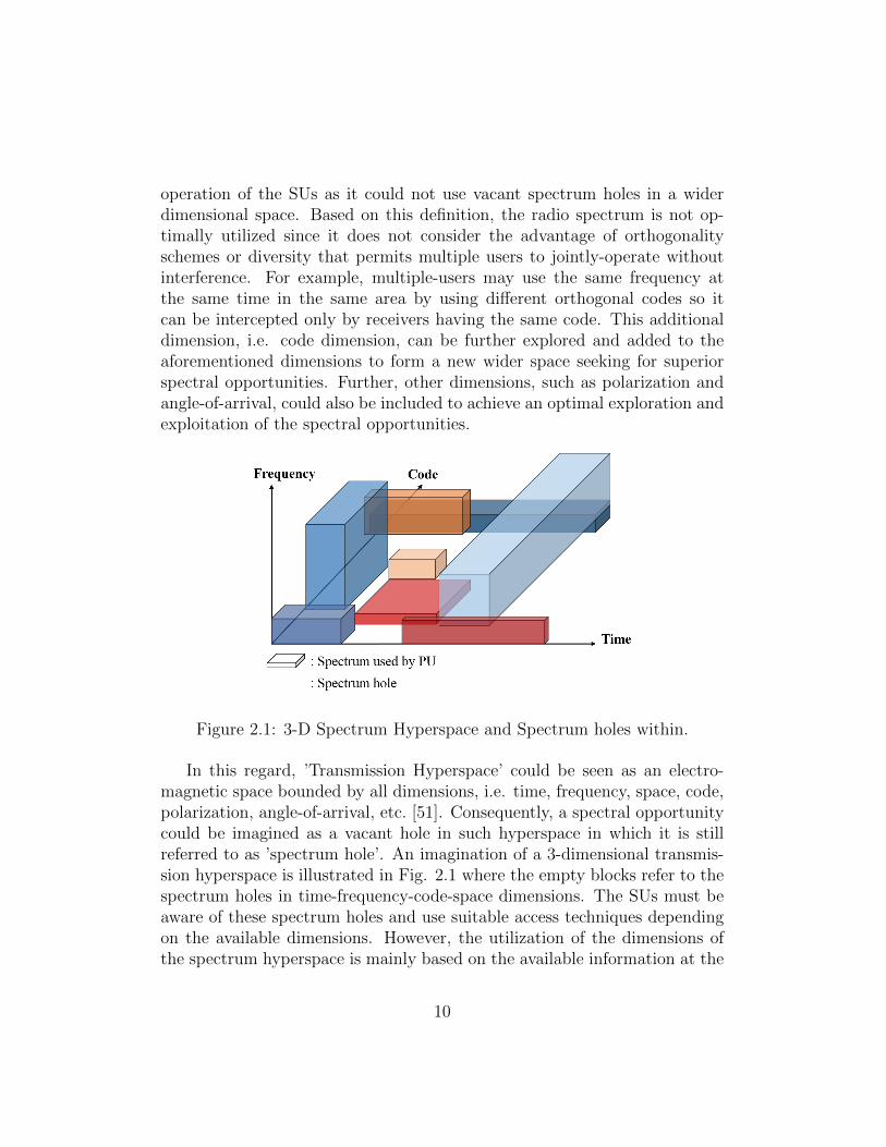
operation of the SUs as it could not use vacant spectrum holes in a widerdimensional space. Based on this definition, the radio spectrum is not op-timally utilized since it does not consider the advantage of orthogonalityschemes or diversity that permits multiple users to jointly-operate withoutinterference. For example, multiple-users may use the same frequency atthe same time in the same area by using different orthogonal codes so itcan be intercepted only by receivers having the same code. This additionaldimension, i.e. code dimension, can be further explored and added to theaforementioned dimensions to form a new wider space seeking for superiorspectral opportunities. Further, other dimensions, such as polarization andangle-of-arrival, could also be included to achieve an optimal exploration andexploitation of the spectral opportunities.
Figure 2.1: 3-D Spectrum Hyperspace and Spectrum holes within.
In this regard, ’Transmission Hyperspace’ could be seen as an electro-magnetic space bounded by all dimensions, i.e. time, frequency, space, code,polarization, angle-of-arrival, etc. [51]. Consequently, a spectral opportunitycould be imagined as a vacant hole in such hyperspace in which it is stillreferred to as ’spectrum hole’. An imagination of a 3-dimensional transmis-sion hyperspace is illustrated in Fig. 2.1 where the empty blocks refer to thespectrum holes in time-frequency-code-space dimensions. The SUs must beaware of these spectrum holes and use suitable access techniques dependingon the available dimensions. However, the utilization of the dimensions ofthe spectrum hyperspace is mainly based on the available information at the
10
SUs. Here, the awareness needs not only the necessary information about thepresence/absence of the PU in certain channels but also necessitates to iden-tify the PU’s waveform (e.g. radio access techniques, chip rates, preambles,etc.) and others [52]. Important dimensions of the transmission hyperspaceare summarized in the following:
• Frequency Dimension: Frequency dimension is usually subdivided intospectrum bands that are typically matching the channelization of par-ticular services such as the frequency division multiple access (FDMA)scheme [53]. Spectral opportunities, in this dimension, are the spec-trum bands that are not utilized by the PUs.
• Time Dimension: The time dimension, depending on the application, issubdivided into periods such as the time-slots structure in time divisionmultiple access (TDMA) systems [53]. Hence, SUs must be aware of thespectral opportunities available in the time domain, i.e. periods of timethe spectrum band is not occupied with respect to other dimensions.
• Space Dimension: The space dimension refers to the physical geograph-ical location and distance of PUs. As early discussed, the spectrum isunder-utilized in the spatial domain. Hence, at a certain location, thespectrum may be unoccupied while it is occupied at another. Hence,spectrum opportunities could be found in some parts of the space di-mension in which SUs can exploit.
• Angle-of-Arrival Dimension: Using advances in multiple-antenna tech-nology, such as beamforming, the SUs can simultaneously use the samespectrum band with the PUs at the same time in the same locationbut through different direction than the direction of the PU radio sig-nal [54]. This is usually known as the angle-of-arrival transmission inwhich different transmitters can simultaneously operate on the samefrequency without interfering by forming the transmission beam in thedirection of the intended receiver. Hence, a new spectral opportunitycould be exploited if the SUs are aware of the position of the PU alongwith its beam direction (i.e. azimuth and elevation angle).
• Code Dimension: The spectrum may be used at a particular time andin a particular location and still could be considered as a spectral op-portunity which might be used by the SUs thanks to the code division
11
access technique [53]. However, this assumes that both primary andsecondary networks are using different orthogonal codes in which mul-tiple PUs and/or SUs can access simultaneously the spectrum bandwithout interfering. Accordingly, the SUs must be aware of the codingtechnology used (e.g. frequency-hopping, direct-sequence etc.) and thecodes used by the PUs.
• Polarization Dimension: The electric field propagation determines thepolarization of the electromagnetic wave. In general, most antennasradiate either linear (i.e. horizontal or vertical) polarization or circular(i.e. right-hand-circular or left-hand-circular) polarization. If the SUsare aware of the polarization state of the PUs, then it can transmitsimultaneously in polarization state other than the polarization of thePUs as it is not causing harmful interference. The reader can referto [55,56] for examples on polarization exploitation in CRs.
Consequently, spectrum sensing must consider all the transmission hy-perspace dimensions for an optimal utilization. From spectrum utilizationefficiency perspective, the more dimensions the SUs are exploring the moreefficient is the utilization of the spectrum holes and hence, a higher successlevel of the CR objective is achieved. In this regard, the focus of this the-sis is the EBD using multiple antenna technology as discussed in Sec. 2.5.This detector allows the SUs to be aware of the spectrum holes in the time,frequency, space and angle-of-arrival dimensions.
2.3 Spectrum Sensing: Behind the Concept
Spectrum scarcity and under-utilization are the main motivations behind theconcept of CR technology. To overcome these spectrum shortage problems,several spectrum exploitation models were proposed: (i) dynamic exclusiveuse model which include certain flexibility to improve spectrum efficiencywhile maintaining on the basic structure of the current spectrum allocationpolicy [57,58] and (ii) spectrum commons model which consists of a spectrumband for sharing between different users [59, 60]. These models improve thespectrum efficiency by providing unlicensed shared bands or an access to thelicensed band for a certain time under the supervision of the primary network.However, the spectrum holes are still not exploited and the licensed bandsare still considered underutilized.
12
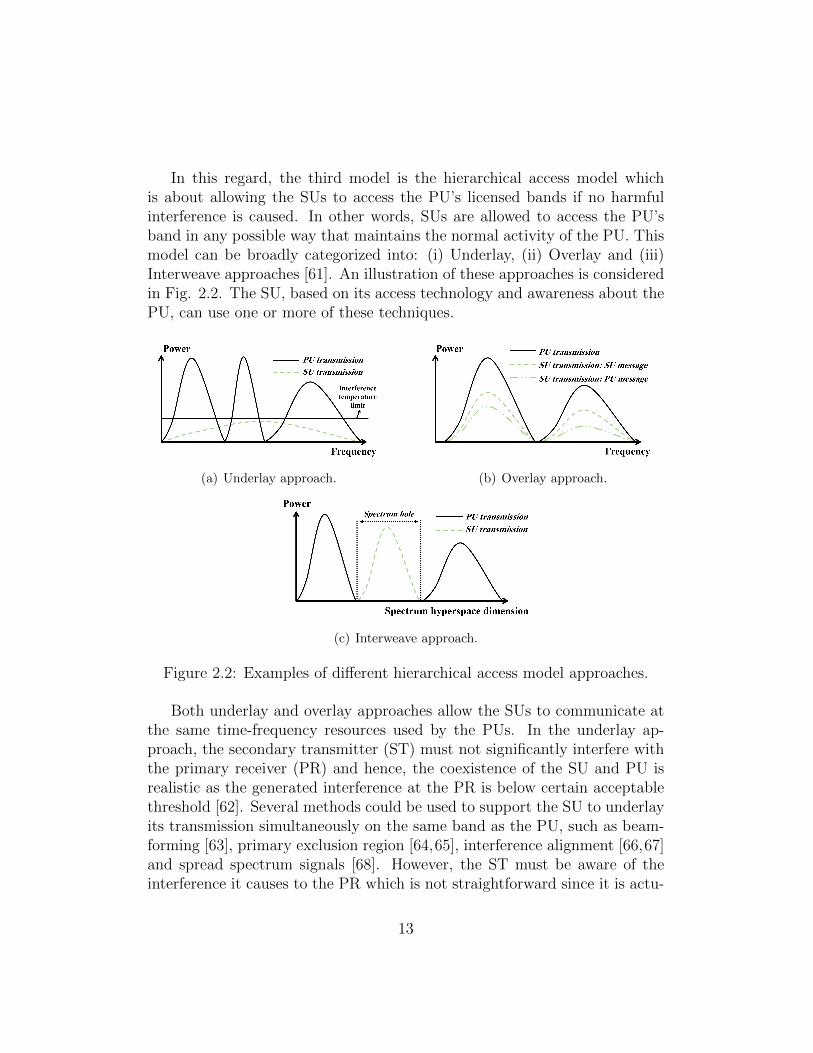
In this regard, the third model is the hierarchical access model whichis about allowing the SUs to access the PU’s licensed bands if no harmfulinterference is caused. In other words, SUs are allowed to access the PU’sband in any possible way that maintains the normal activity of the PU. Thismodel can be broadly categorized into: (i) Underlay, (ii) Overlay and (iii)Interweave approaches [61]. An illustration of these approaches is consideredin Fig. 2.2. The SU, based on its access technology and awareness about thePU, can use one or more of these techniques.
(a) Underlay approach. (b) Overlay approach.
(c) Interweave approach.
Figure 2.2: Examples of different hierarchical access model approaches.
Both underlay and overlay approaches allow the SUs to communicate atthe same time-frequency resources used by the PUs. In the underlay ap-proach, the secondary transmitter (ST) must not significantly interfere withthe primary receiver (PR) and hence, the coexistence of the SU and PU isrealistic as the generated interference at the PR is below certain acceptablethreshold [62]. Several methods could be used to support the SU to underlayits transmission simultaneously on the same band as the PU, such as beam-forming [63], primary exclusion region [64,65], interference alignment [66,67]and spread spectrum signals [68]. However, the ST must be aware of theinterference it causes to the PR which is not straightforward since it is actu-
13
ally happens at the PR side. In the overlay approach, the STs use advancedtechniques in coding and transmission in order to mitigate the interferencecaused by such transmission. Basically, as shown in Fig. 2.2(b), the STsmust relay the primary signals by using part of their power and the rest areused to transmit their own signals [61]. Accordingly, overlay approach needsadvanced techniques in precoding, transmission and perfect power splitting,interference mitigation and time and frequency synchronization. Moreover,it also requires PU-SU cooperation, non-causal prior knowledge about thePU and could not be applied except in very few cases [69].
On the other hand, interweave approach is about the opportunistic uti-lization of the spectrum holes whenever and wherever it exists. It was thebasic motivation behind the introduction of the CR systems as a solution forthe under-utilization problem of the licensed spectrum bands. The SUs, inthis approach, must be aware of the PU activity in its geographical area inorder to identify the spectrum holes and exploit them for their own transmis-sion. Further, SUs must also identify any reappearance of the PU and should,immediately, leave the channel by switching to another spectrum hole or stoptransmission. This opportunistic use of the spectrum, ideally, causes no inter-ference to the PU. Indeed, this is almost true if the used awareness methodis capable of correctly identifying the spectrum hole with optimal perfor-mance. However, any incorrect identification will lead to a miss-utilizationof the spectrum hole or harmful interference to the PU. Consequently, theperformance of the awareness mechanism is a challenge in the interweaveapproach.
In general, most of the aforementioned exploitation techniques could bejointly used. For example, SUs can underlay their transmission until a spec-trum hole is detected and then shift to the interweave approach to transmitwith higher power according to the dimensions of the spectrum hole. How-ever, interweave is the most efficient and effective approach for exploiting theunderutilized spectrum by targeting the spectrum holes in the transmissionhyperspace. In this regard, different spectrum awareness methods exist inorder to serve the SUs and make them aware of the surrounding environ-ment. On a large scale, spectrum awareness can be classified into passiveand active awareness [70]. In passive awareness, the SU receives the spectralinformation needed from an outside agent. On the other hand, in activeawareness the SUs need to sense the radio environment and make their ownmeasurements.
Different passive awareness techniques are proposed to inform the SU
14
about its surrounding spectrum status. Such techniques include (i) Bea-con Signals [71–73], (ii) Control Channel [74–78], (iii) Geolocation databases[79–82], (iv) Policy based [83] and (v) Spectrum broker [71]. In fact, pas-sive awareness can ensure interference-free communication to the PUs and asimple secondary transceiver. However, it may require modification to thePU systems, control channels and the establishment of costly infrastructure.Moreover, passive awareness leads to a static SU that strongly depends onhow frequent the outside agent is updated. On the other hand, active aware-ness could be either detecting a PR or a PT. Methods for detecting the PRare based on detecting the Local Oscillator (LO) leakage power [10, 84] orthe interference at the PR [85]. Since LO leakage and interference are actu-ally happening at the receiver side, then CR active awareness based on theseapproaches must focus on the receiver activity of the PU. To fulfill such ap-proach, it is more likely that the secondary network should establish a largegrid of sensors to cover all its communication region. Hence, without PU-SUcooperation assumption, it is easier to detect the PT than the detection ofPR. In this regard, Spectrum sensing (SS) is the active awareness approachthat is responsible on detecting the PT by taking certain measures from theSU surrounding environment and decide whether a spectrum hole exists ornot. The main advantage of SS approach is that the SUs may not need to relyon any external source of knowledge to take a transmit/no-transmit decision.
Based on this discussion, SS is considered as the most practical, effi-cient and effective approach in spectrum awareness. It permits the detectionof spectrum holes in order to be exploited using the interweave approach.This concept is basic in CR since it takes the spectrum bands from the un-derutilized state to a more efficiently-utilized state. There exists a massivenumber of researches that provide this approach with worthy different de-tection techniques to identify the spectrum holes. In the next section, wediscuss the concept of SS and different aspects related to it.
2.4 Spectrum Sensing: literature review
Spectrum sensing is a crucial stage that must be performed by the SUs inorder to identify the spectrum holes. To this end, a variety of techniqueshas been proposed in literature. In general, these techniques are based on
15
detection problem with binary hypothesis model defined as:
H0 : y(n) = η(n), (2.1)
H1 : y(n) = s(n) + η(n), (2.2)
where y(n) is the sample received at instant n; η(n) represents the additivewhite Gaussian noise with zero mean and variance σ2
η; s(n) is the PU’s trans-mitted signal samples passed through a wireless channel. This represents abinary signal detection problem in which SUs need to decide between thetwo hypotheses, H0 or H1. H0 is the only noise hypothesis, i.e. the PU doesnot exist, while H1 indicates that the considered spectrum band is occupied.
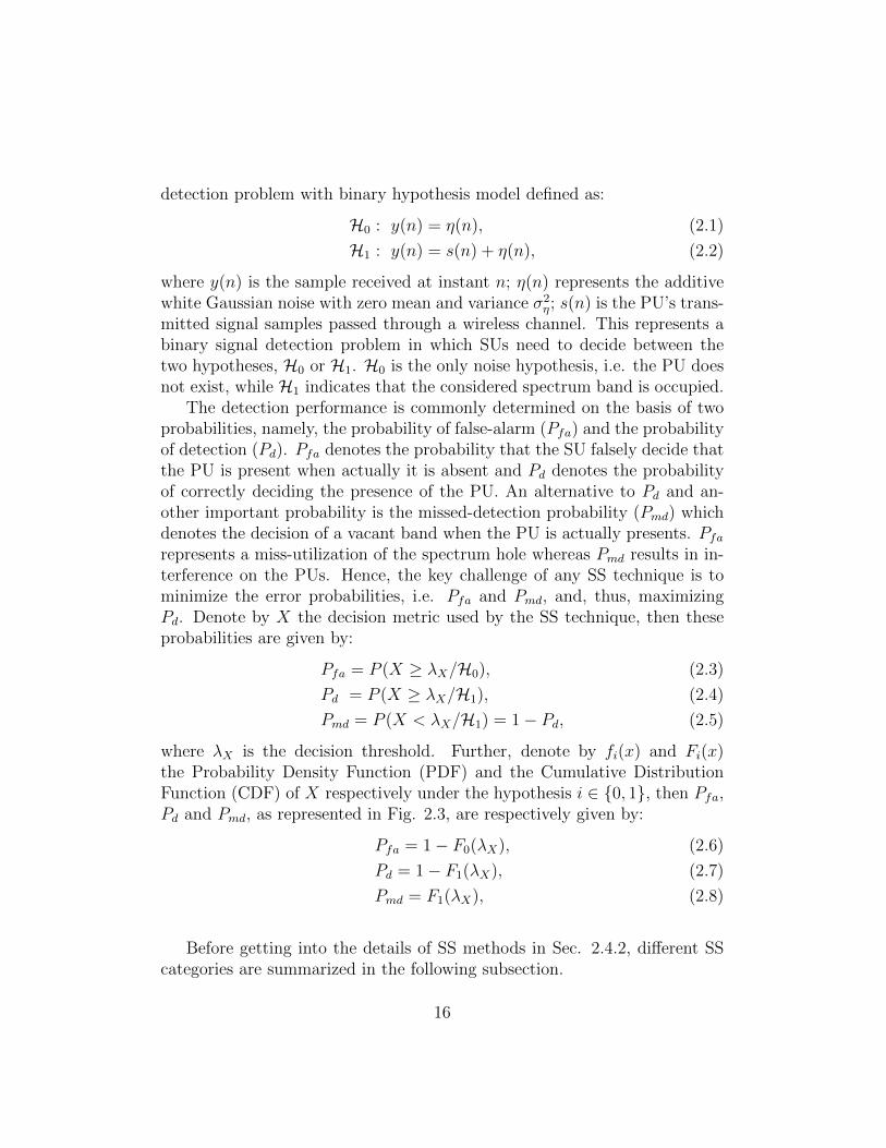
The detection performance is commonly determined on the basis of twoprobabilities, namely, the probability of false-alarm (Pfa) and the probabilityof detection (Pd). Pfa denotes the probability that the SU falsely decide thatthe PU is present when actually it is absent and Pd denotes the probabilityof correctly deciding the presence of the PU. An alternative to Pd and an-other important probability is the missed-detection probability (Pmd) whichdenotes the decision of a vacant band when the PU is actually presents. Pfarepresents a miss-utilization of the spectrum hole whereas Pmd results in in-terference on the PUs. Hence, the key challenge of any SS technique is tominimize the error probabilities, i.e. Pfa and Pmd, and, thus, maximizingPd. Denote by X the decision metric used by the SS technique, then theseprobabilities are given by:
Pfa = P (X ≥ λX/H0), (2.3)
Pd = P (X ≥ λX/H1), (2.4)
Pmd = P (X < λX/H1) = 1− Pd, (2.5)
where λX is the decision threshold. Further, denote by fi(x) and Fi(x)the Probability Density Function (PDF) and the Cumulative DistributionFunction (CDF) of X respectively under the hypothesis i ∈ 0, 1, then Pfa,Pd and Pmd, as represented in Fig. 2.3, are respectively given by:
Pfa = 1− F0(λX), (2.6)
Pd = 1− F1(λX), (2.7)
Pmd = F1(λX), (2.8)
Before getting into the details of SS methods in Sec. 2.4.2, different SScategories are summarized in the following subsection.
16
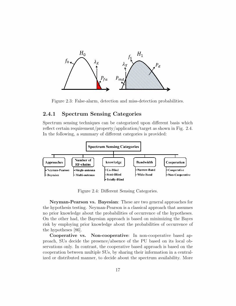
Figure 2.3: False-alarm, detection and miss-detection probabilities.
2.4.1 Spectrum Sensing Categories
Spectrum sensing techniques can be categorized upon different basis whichreflect certain requirement/property/application/target as shown in Fig. 2.4.In the following, a summary of different categories is provided:
Figure 2.4: Different Sensing Categories.
Neyman-Pearson vs. Bayesian: These are two general approaches forthe hypothesis testing. Neyman-Pearson is a classical approach that assumesno prior knowledge about the probabilities of occurrence of the hypotheses.On the other had, the Bayesian approach is based on minimizing the Bayesrisk by employing prior knowledge about the probabilities of occurrence ofthe hypotheses [86].
Cooperative vs. Non-cooperative: In non-cooperative based ap-proach, SUs decide the presence/absence of the PU based on its local ob-servations only. In contrast, the cooperative based approach is based on thecooperation between multiple SUs, by sharing their information in a central-ized or distributed manner, to decide about the spectrum availability. More
17
about cooperation is provided by Sec. 2.4.3.Un-blind vs. Semi-blind vs. Totally-blind: These categories reflect
the amount of prior knowledge required at the SU. Un-blind detectors requirea prior knowledge about the PU signal’s characteristics as well as the noisepower to accurately make a decision. Semi-blind detectors are more practicalas they require a prior knowledge about the noise power only. This powercould be estimated, however, a further performance study for such detectorsin the presence of noise uncertainty is required. On the other hand, totally-blind detectors are the detectors that do not require any prior informationregarding both the PU signal and the noise power. These techniques are themost practical and preferable techniques in SS.
Multi-antenna vs. Single-antenna: It is about the number of anten-nas at the RF part of the SU that are used for the SS process. In comparisonwith single-antenna SS, multi-antenna SS utilize the spatial correlation of PUsignal received by different antennas for spectrum holes detection. Moreover,several multi-antenna SS techniques have been shown to be totally-blind andthus, provide robustness against noise uncertainty problems. On the otherhand, multi-antenna SS requires additional hardware components and anincrease in the computational complexity. More about multi-antenna is pro-vided by Sec. 2.4.4.
Wide-band vs. Narrow-band: Herein, the detectors are categorizedbased on the bandwidth of the channel to be sensed. Narrow-band (NB)SS techniques are detectors that could be used to sense a sufficiently narrowfrequency range band such that a flat channel frequency response could beconsidered, i.e. the sensed bandwidth is less than the channel coherencebandwidth [87]. On the other hand, wide-band (WB) SS techniques aim tosense a wider frequency band. It is worth noting that the NB SS techniquescannot be directly used in WB sensing, however, they can be extended forWB context.
In addition, categories, such as proactive (i.e. periodic sensing) or re-active (i.e. on-demand sensing), In-band (i.e. sensing the band currentlyused by the SUs) or Out-of-band (i.e. sensing other bands for possiblebackup) and sequential (i.e. sensing several bands sequentially) or parallel(i.e. sensing several bands in parallel), also exists. However, the fundamentalof all these categories is to detect the spectrum holes in order to be used bythe SUs. In this regard, different methods were proposed in literature andare discussed next.
18
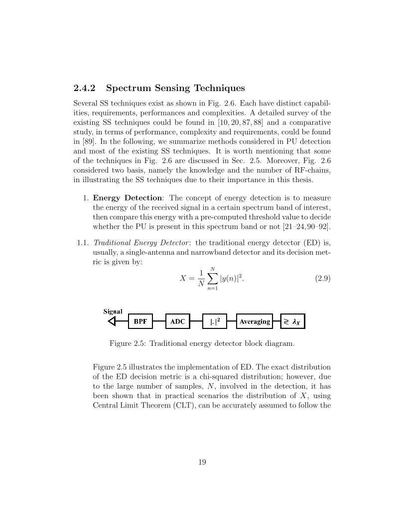
2.4.2 Spectrum Sensing Techniques
Several SS techniques exist as shown in Fig. 2.6. Each have distinct capabil-ities, requirements, performances and complexities. A detailed survey of theexisting SS techniques could be found in [10, 20, 87, 88] and a comparativestudy, in terms of performance, complexity and requirements, could be foundin [89]. In the following, we summarize methods considered in PU detectionand most of the existing SS techniques. It is worth mentioning that someof the techniques in Fig. 2.6 are discussed in Sec. 2.5. Moreover, Fig. 2.6considered two basis, namely the knowledge and the number of RF-chains,in illustrating the SS techniques due to their importance in this thesis.
1. Energy Detection: The concept of energy detection is to measurethe energy of the received signal in a certain spectrum band of interest,then compare this energy with a pre-computed threshold value to decidewhether the PU is present in this spectrum band or not [21–24,90–92].
1.1. Traditional Energy Detector : the traditional energy detector (ED) is,usually, a single-antenna and narrowband detector and its decision met-ric is given by:
X =1
N
N∑n=1
|y(n)|2. (2.9)
Figure 2.5: Traditional energy detector block diagram.
Figure 2.5 illustrates the implementation of ED. The exact distributionof the ED decision metric is a chi-squared distribution; however, dueto the large number of samples, N , involved in the detection, it hasbeen shown that in practical scenarios the distribution of X, usingCentral Limit Theorem (CLT), can be accurately assumed to follow the
19
Gaussian distribution [93]. Consequently, one can obtain the following:
H0 : X ∼ N(σ2η,σ4η
N
), (2.10)
H1 : X ∼ N(σ2η + σ2
s ,(σ2
η + σ2s)
2
N
), (2.11)
where σ2s is the energy of the signal at the SR (i.e. including chan-
nel effect). Hence, Pfa, Pd and Pmd, using (2.6), (2.7) and (2.8), arestraightforwardly formulated as follows:
Pfa = Q
(λX − σ2
η
σ2η/√N
), (2.12)
Pd = Q
(λX − σ2
η(1 + ρ)
σ2η(1 + ρ)/
√N
). (2.13)
where Q(.) is the standard Gaussian complementary CDF and ρ is thesignal to noise ratio. The optimal decision threshold, λX , is selected byminimizing both Pfa and Pmd. However, this requires the knowledge ofnoise and received signal powers.
ED is the most popular technique for SS due to its low implementationand computational complexities. In practice, the threshold is chosenso as to maintain a predefined false-alarm probability, i.e. ConstantFalse Alarm Rate (CFAR) [94]. Hence, ED is considered a semi-blinddetector as it is sufficient to know the noise variance for calculating λX .Despite the simplicity of ED, its main drawback lies in its sensitivity onnoise power uncertainty. Any small error in the noise power estimationmay cause a significant performance degradation.
The threshold of the ED, for a CFAR, is straightforward from (2.12)as:
λX = σ2η
(1 +
Q−1(Pfa)√N
), (2.14)
where Q−1(.) is the inverse Q-function. In perfect operating conditions,i.e. σ2
η is perfectly known, ED can achieve any detection performanceby increasing N . For a targeted Pfa and Pd, the minimum required Nis straightforward derived from (2.12) and (2.13) as:
N =[Q−1(Pfa)−Q−1(Pd)(1 + ρ)
].ρ−2. (2.15)
20
Hence, if σ2η is known, the ED can detect any PU at arbitrarily low
SNR by increasing N . Conversely, due to noise uncertainty the PUcould not be detected if the SNR is under certain SNR wall regardlessthe value of N [95,96]. To address this issue, accurate noise estimationmethods [91,97] and hybrid detectors [98] were proposed for ED.
1.2. Teager-Kaiser based ED : As presented for the ED, the most widelyused approach for the energy estimation is based on the squared energyoperator whereby the desired energy given by (2.9) or the squares ofthe magnitude of the frequency samples of the same signal segmentafter discrete Fourier transform (DFT). Alternatively, a simple and fastapproach is based on the Teager-Kaiser energy operator which was firstproposed by Teager in [99] and further investigated by Kaiser [100]. Acomparison between both energy estimation approaches in presence ofadditive noise is reported in [101]. In CR, Teager-Kaiser based ED hasbeen used in detecting the wireless microphone signals in narrowbandand wideband frequency domains [24,92].
2. Feature Detection:
In general, Feature Detector (FD) distinguishes the PU by matchingfeatures extracted from the received signal with a priori known featuresthat characterize the PU transmission such as Cyclostationarity, idleguard interval of OFDM, location, channel bandwidth and its shape,etc. [25–31,98,102–107].
2.1 Cyclostationary Feature Detector: Cyclostationary Feature De-tector (CFD) is an effective FD that exploits the cyclostationary fea-tures of the primary signals [27–31, 98, 102–107]. Unlike the noise, PUsignals are modulated signals that carry cyclostationary features dueto the periodicity in its statistics such as the mean and the autocor-relation. In this regard, the cyclic spectrum density (CSD) functionis defined as the Fourier series expansion of the cyclic autocorrelationfunction of the received signal. If PU is present, the CSD functionshows peak values when the cyclic frequencies are equal to the funda-mental frequencies of the PU signals. This approach is robust againstnoise uncertainty and shows high detection performance at the costof high computational complexity. However, CFD is very sensitive tocyclic frequency mismatch [108].
21
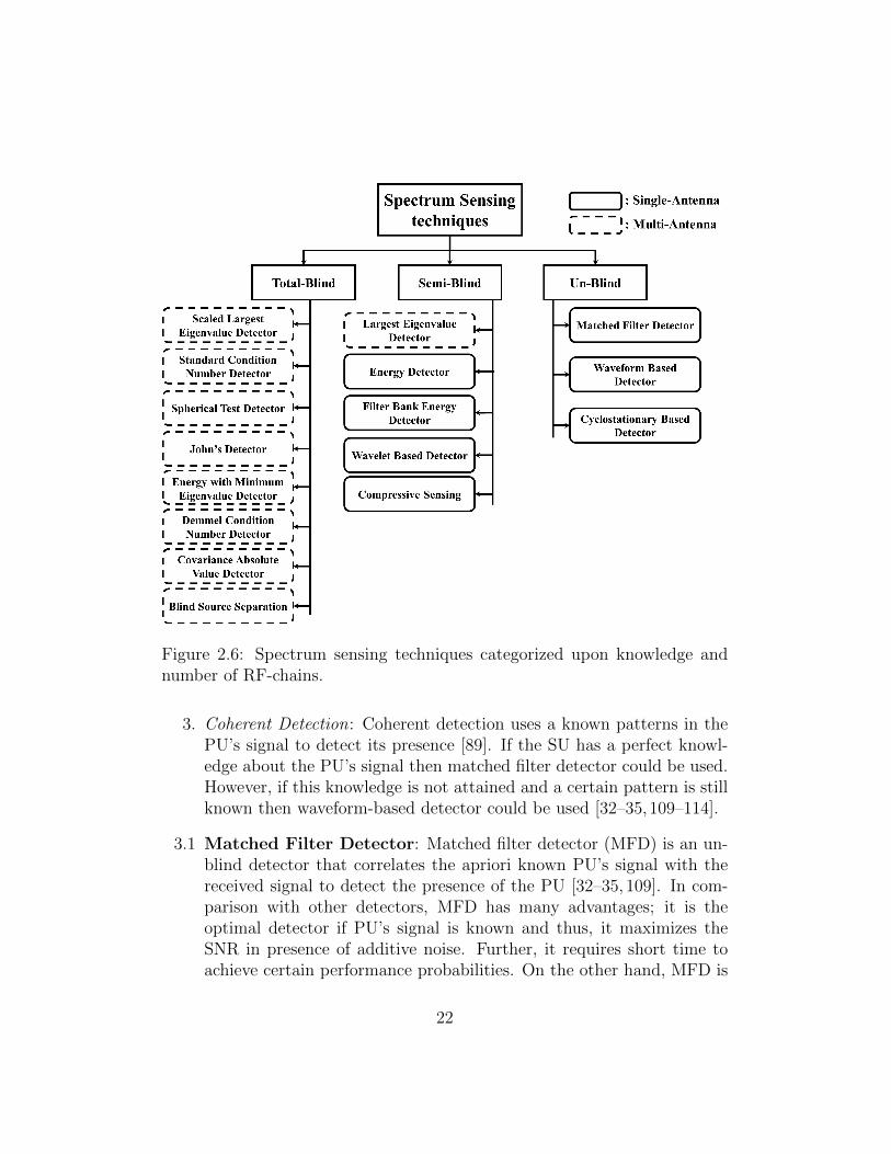
Figure 2.6: Spectrum sensing techniques categorized upon knowledge andnumber of RF-chains.
3. Coherent Detection: Coherent detection uses a known patterns in thePU’s signal to detect its presence [89]. If the SU has a perfect knowl-edge about the PU’s signal then matched filter detector could be used.However, if this knowledge is not attained and a certain pattern is stillknown then waveform-based detector could be used [32–35,109–114].
3.1 Matched Filter Detector: Matched filter detector (MFD) is an un-blind detector that correlates the apriori known PU’s signal with thereceived signal to detect the presence of the PU [32–35, 109]. In com-parison with other detectors, MFD has many advantages; it is theoptimal detector if PU’s signal is known and thus, it maximizes theSNR in presence of additive noise. Further, it requires short time toachieve certain performance probabilities. On the other hand, MFD is
22

not considered as relevant choice in CR due to several disadvantages;first, MFD requires perfect knowledge of PU’s signal features such asoperating frequency, bandwidth, modulation, pulse shaping etc. andthus, it suffers from high performance degradation if wrong informationregarding PU signal is used in the detection. Moreover, its implemen-tation complexity is impractically large as it needs a dedicated receiverfor every primary system type which also results in high power con-sumption.
3.2 Waveform-Based Detector: Pilots, spreading codes, preambles andmidambles are examples of patterns used by most wireless communi-cation systems for synchronization, equalization and other purposes.If PU signal features are not perfectly known by the SU, such pat-terns might still be a priori known. Waveform-based detector corre-lates the received signal with a copy of the known pattern for PUdetection [110, 111]. The performance of this detector improves as thelength of the known pattern increases. It can be seen as a simplified ver-sion of MFD however, synchronization between the primary signal andthe detector is still required and thus, any synchronization error candegrade the detection performance. Moreover, SUs must have knowl-edge of patterns of all primary system in its coverage area. Cyclic prefixcorrelation detector [112, 113] and pilot detector [114] are examples ofwaveform-based detector.
4. Covariance Based Detection: Covariance based approach is based onthe sample covariance matrix of the received signal at the SR in whichit exploits the difference in the statistical covariances of the receivedsignal and the noise.
4.1 Covariance Absolute Value Detector: In the covariance based ap-proach, the authors in [115] proposed Covariance Absolute Value (CAV)detector which is a totally-blind detector that rely on the fact that ifPU is not present then the off-diagonal elements of the covariance ma-trix are all zeros whereas if the PU’s signal exists and the samples arecorrelated then the covariance matrix is not diagonal. The distributionof the ratio of the sum of absolute values of the non-diagonal elementsto that of the diagonal elements were further studied in [116] in orderto obtain mathematical expressions for the Pfa and Pd.
23
4.2 Eigenvalue Based Detector: Eigenvalue based detector (EBD) couldbe considered as an advanced method in the covariance based detectionapproach. It relies on the eigenvalues of the sample covariance ma-trix of the signal received using certain diversity technique such as thefractional sampling, cooperation or multi-antenna [36–43, 117]. EBDconsists of several detection techniques whose properties are studiedusing recent results from advances in random matrix theory (RMT).Some of the these techniques are totally-blind and outperform the EDespecially in noise uncertain environment. A detailed description ofthis approach is provided in Sec. 2.5.
5. Wide-Band Detection: Two main approaches in wide-band SS are theNyquist wide-band SS and the sub-Nyquist wide-band SS [87]. InNyquist Wide-band SS, the signal is directly acquired using a high sam-pling rate analog-to-digital converter (ADC), i.e. at or above Nyquistrate, and then uses some signal processing techniques to detect the spec-trum holes. In contrast, sub-Nyquist wide-band SS detects the spec-trum holes using acquisitions at sampling rate lower than the Nyquistrate. Various wide-band techniques were proposed in literature andused in SS such as:
5.1 Compressive Sensing: Compressive sensing is a powerful approachthat enables the analysis and recovery of a wideband signal while it issampled at a sub-Nyquist rate [27, 98, 118–123]. Compressive sensingexploits the fact that many natural signals are sparse or compress-ible and can be represented shortly when expressed in a proper ba-sis. Sparsity represents the property that the ”information rate” ofa continuous-time signal could be much smaller than proposed by itsbandwidth [118].
5.2 Wavelet Based Detector: Wavelet detection is an effective techniqueused in image processing for edge detection. In SS, wavelet detectionis applied on the wideband power spectral density (PSD) to detect theedges which represents the transitions between occupied and vacantbands [124]. Once the edges are detected, the bands between the edgesare further analyzed to identify the spectrum holes.
5.3 Filter-Bank Based Detector: In multi-carrier communication sys-tems, spectrum sensing can be performed by measuring the power at
24
the output of the sub-carrier bands [125]. In this regard, MultitaperBased Detector can be seen as a filter-bank spectrum estimation withmultiple filter banks or filter-bank is a simplified version of the multi-taper by using only one prototype filter for each band [10,126,127].
6. Examples of Other Detectors : In addition to the mentioned techniques,other detectors also exists. The reader may refer to the surveys such as[10,20] for others detection techniques. Here we refer for two examples:
6.1 Blind Source Separation detection: Blind Source Separation (BSS)was recently proposed in CR networks for SS [128–130]. Several meth-ods were used to separate the mixed signal of CR with the PU or tosense multi frequency bands by separating different signals in differentfrequency bands such as the independent component analysis [129] andthe Kurtosis applied on the separated signals [130]. The advantage ofsuch techniques is their ability to sense the channel even if the SU isoperating. However, BSS assumes the statistical independence of thesources. Moreover, other detectors, like EBD, are used with the BSSto improve its performance [130].
6.2 High-order statistics based detection: High-order statistics rep-resent the third and higher order in which two basic statistics the mo-ments and cumulants exist. While the first-order and second-orderstatistics are used to detect the signals in most of the CR applica-tions, high-order moment based detectors have been considered to de-tect signals have certain properties. For example, second-, fourth- andsix-order moments were used in [131], ratio of the second and fourthmoments were used in [132] and the third- and higher odd momentswere used in [133].
2.4.3 Cooperation in Spectrum Sensing
In general, any wireless communication channel may be characterized bymulti-path fading, path-loss, shadowing, noise uncertainty and interferencein which the detection performance of the SS techniques may significantlydegrade. To overcome these challenges, cooperative sensing was proposedto enhance the detection performance by exploiting the spatial location ofdifferent SUs. By means of cooperation, SUs sense certain spectrum bandand share their sensing information toward achieving a combined and more
25
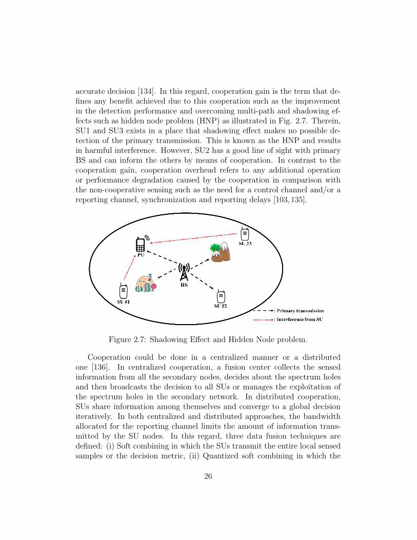
accurate decision [134]. In this regard, cooperation gain is the term that de-fines any benefit achieved due to this cooperation such as the improvementin the detection performance and overcoming multi-path and shadowing ef-fects such as hidden node problem (HNP) as illustrated in Fig. 2.7. Therein,SU1 and SU3 exists in a place that shadowing effect makes no possible de-tection of the primary transmission. This is known as the HNP and resultsin harmful interference. However, SU2 has a good line of sight with primaryBS and can inform the others by means of cooperation. In contrast to thecooperation gain, cooperation overhead refers to any additional operationor performance degradation caused by the cooperation in comparison withthe non-cooperative sensing such as the need for a control channel and/or areporting channel, synchronization and reporting delays [103,135].
Figure 2.7: Shadowing Effect and Hidden Node problem.
Cooperation could be done in a centralized manner or a distributedone [136]. In centralized cooperation, a fusion center collects the sensedinformation from all the secondary nodes, decides about the spectrum holesand then broadcasts the decision to all SUs or manages the exploitation ofthe spectrum holes in the secondary network. In distributed cooperation,SUs share information among themselves and converge to a global decisioniteratively. In both centralized and distributed approaches, the bandwidthallocated for the reporting channel limits the amount of information trans-mitted by the SU nodes. In this regard, three data fusion techniques aredefined: (i) Soft combining in which the SUs transmit the entire local sensedsamples or the decision metric, (ii) Quantized soft combining in which the
26
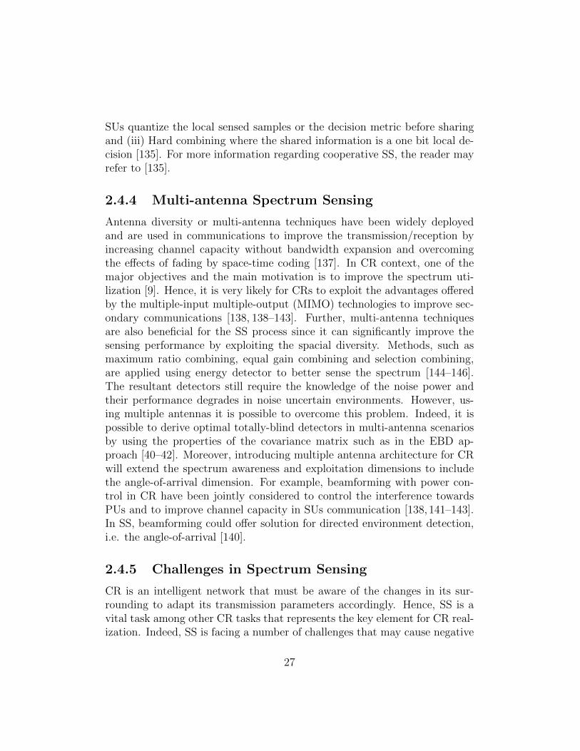
SUs quantize the local sensed samples or the decision metric before sharingand (iii) Hard combining where the shared information is a one bit local de-cision [135]. For more information regarding cooperative SS, the reader mayrefer to [135].
2.4.4 Multi-antenna Spectrum Sensing
Antenna diversity or multi-antenna techniques have been widely deployedand are used in communications to improve the transmission/reception byincreasing channel capacity without bandwidth expansion and overcomingthe effects of fading by space-time coding [137]. In CR context, one of themajor objectives and the main motivation is to improve the spectrum uti-lization [9]. Hence, it is very likely for CRs to exploit the advantages offeredby the multiple-input multiple-output (MIMO) technologies to improve sec-ondary communications [138, 138–143]. Further, multi-antenna techniquesare also beneficial for the SS process since it can significantly improve thesensing performance by exploiting the spacial diversity. Methods, such asmaximum ratio combining, equal gain combining and selection combining,are applied using energy detector to better sense the spectrum [144–146].The resultant detectors still require the knowledge of the noise power andtheir performance degrades in noise uncertain environments. However, us-ing multiple antennas it is possible to overcome this problem. Indeed, it ispossible to derive optimal totally-blind detectors in multi-antenna scenariosby using the properties of the covariance matrix such as in the EBD ap-proach [40–42]. Moreover, introducing multiple antenna architecture for CRwill extend the spectrum awareness and exploitation dimensions to includethe angle-of-arrival dimension. For example, beamforming with power con-trol in CR have been jointly considered to control the interference towardsPUs and to improve channel capacity in SUs communication [138, 141–143].In SS, beamforming could offer solution for directed environment detection,i.e. the angle-of-arrival [140].
2.4.5 Challenges in Spectrum Sensing
CR is an intelligent network that must be aware of the changes in its sur-rounding to adapt its transmission parameters accordingly. Hence, SS is avital task among other CR tasks that represents the key element for CR real-ization. Indeed, SS is facing a number of challenges that may cause negative
27
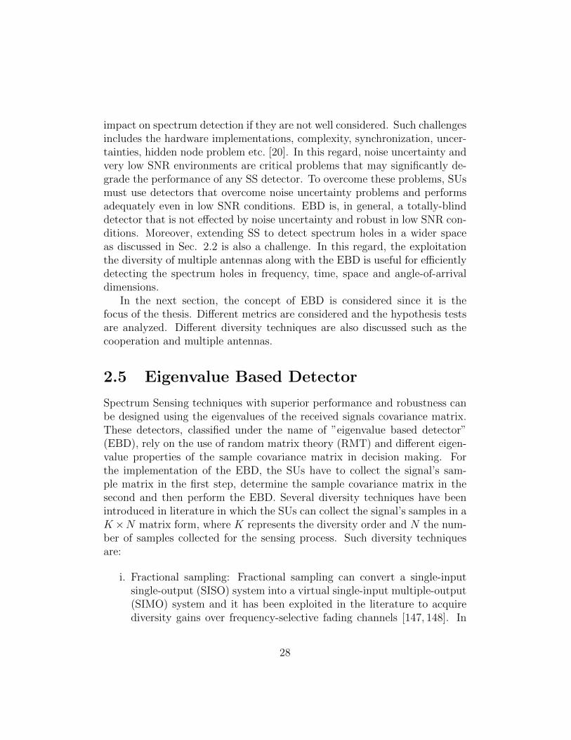
impact on spectrum detection if they are not well considered. Such challengesincludes the hardware implementations, complexity, synchronization, uncer-tainties, hidden node problem etc. [20]. In this regard, noise uncertainty andvery low SNR environments are critical problems that may significantly de-grade the performance of any SS detector. To overcome these problems, SUsmust use detectors that overcome noise uncertainty problems and performsadequately even in low SNR conditions. EBD is, in general, a totally-blinddetector that is not effected by noise uncertainty and robust in low SNR con-ditions. Moreover, extending SS to detect spectrum holes in a wider spaceas discussed in Sec. 2.2 is also a challenge. In this regard, the exploitationthe diversity of multiple antennas along with the EBD is useful for efficientlydetecting the spectrum holes in frequency, time, space and angle-of-arrivaldimensions.
In the next section, the concept of EBD is considered since it is thefocus of the thesis. Different metrics are considered and the hypothesis testsare analyzed. Different diversity techniques are also discussed such as thecooperation and multiple antennas.
2.5 Eigenvalue Based Detector
Spectrum Sensing techniques with superior performance and robustness canbe designed using the eigenvalues of the received signals covariance matrix.These detectors, classified under the name of ”eigenvalue based detector”(EBD), rely on the use of random matrix theory (RMT) and different eigen-value properties of the sample covariance matrix in decision making. Forthe implementation of the EBD, the SUs have to collect the signal’s sam-ple matrix in the first step, determine the sample covariance matrix in thesecond and then perform the EBD. Several diversity techniques have beenintroduced in literature in which the SUs can collect the signal’s samples in aK×N matrix form, where K represents the diversity order and N the num-ber of samples collected for the sensing process. Such diversity techniquesare:
i. Fractional sampling: Fractional sampling can convert a single-inputsingle-output (SISO) system into a virtual single-input multiple-output(SIMO) system and it has been exploited in the literature to acquirediversity gains over frequency-selective fading channels [147, 148]. In
28
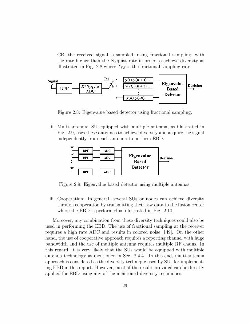
CR, the received signal is sampled, using fractional sampling, withthe rate higher than the Nyquist rate in order to achieve diversity asillustrated in Fig. 2.8 where TFS is the fractional sampling rate.
Figure 2.8: Eigenvalue based detector using fractional sampling.
ii. Multi-antenna: SU equipped with multiple antenna, as illustrated inFig. 2.9, uses these antennas to achieve diversity and acquire the signalindependently from each antenna to perform EBD.
Figure 2.9: Eigenvalue based detector using multiple antennas.
iii. Cooperation: In general, several SUs or nodes can achieve diversitythrough cooperation by transmitting their raw data to the fusion centerwhere the EBD is performed as illustrated in Fig. 2.10.
Moreover, any combination from these diversity techniques could also beused in performing the EBD. The use of fractional sampling at the receiverrequires a high rate ADC and results in colored noise [149]. On the otherhand, the use of cooperative approach requires a reporting channel with hugebandwidth and the use of multiple antenna requires multiple RF chains. Inthis regard, it is very likely that the SUs would be equipped with multipleantenna technology as mentioned in Sec. 2.4.4. To this end, multi-antennaapproach is considered as the diversity technique used by SUs for implement-ing EBD in this report. However, most of the results provided can be directlyapplied for EBD using any of the mentioned diversity techniques.
29

Figure 2.10: Eigenvalue based detector using cooperative technique.
2.5.1 Concept of EBD
Consider a multi-antenna CR system equipped with K receiving antennasaiming to detect the presence/absence of a single PU in a narrowband channelB with the central carrier frequency fc. The received signal at the SR issampled at the sampling frequency fs and denote by N the number of samplesacquired at each antenna for the sensing process. Hence, the sensing time,Ts, is given by: Ts = N/fs and the received signal matrix, Y , is given by:
Y =
y1(1) y1(2) · · · y1(N)y2(1) y2(2) · · · y2(N)
......
. . ....
yK(1) yK(2) · · · yK(N)
, (2.16)
where yk(n) is the baseband sample at antenna k = 1 · · ·K and instantn = 1 · · ·N .
For this detection problem, the received vector, at instant n, under bothhypotheses, H0 and H1, is given by:
H0 : yk(n) = ηk(n),
H1 : yk(n) = hk(n)s(n) + ηk(n),(2.17)
with ηk(n) is a complex circular white Gaussian noise with zero mean andunknown variance σ2
η, hk(n) is the channel coefficient between the PU and
30
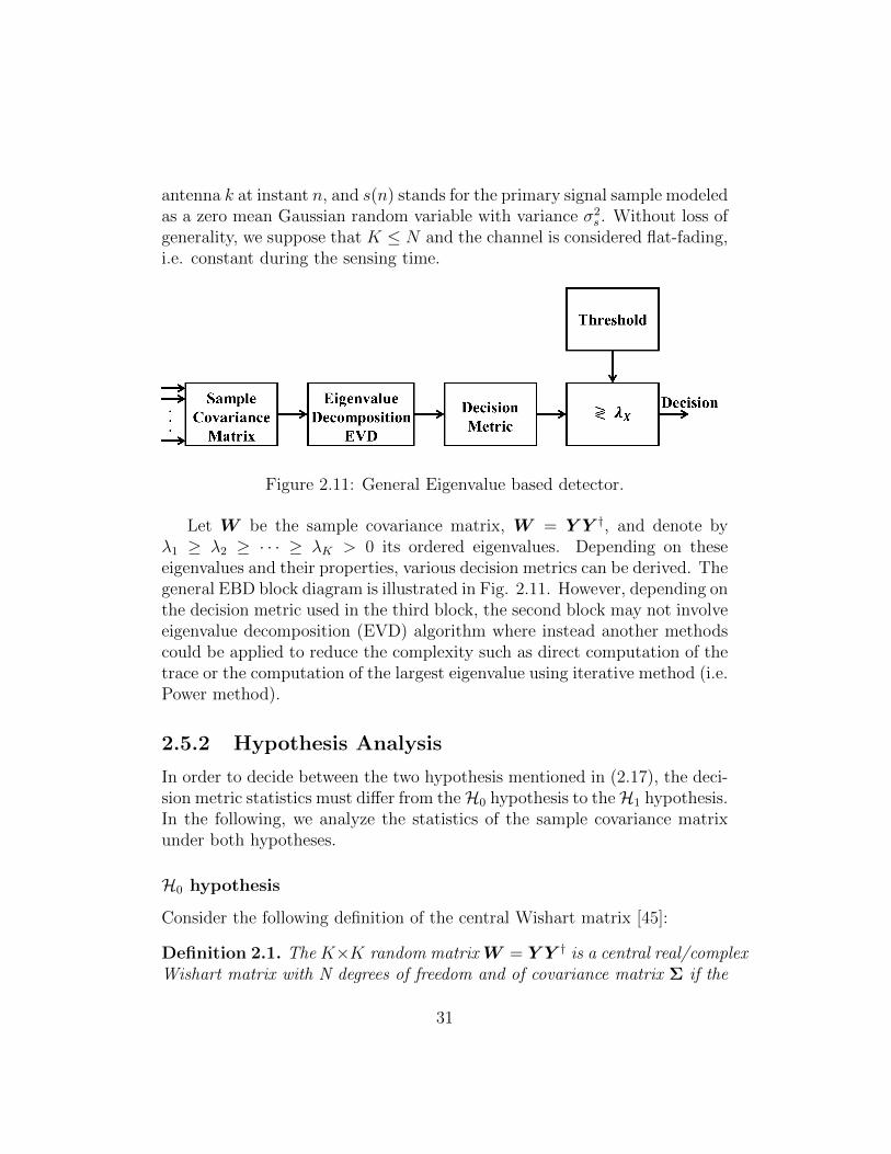
antenna k at instant n, and s(n) stands for the primary signal sample modeledas a zero mean Gaussian random variable with variance σ2
s . Without loss ofgenerality, we suppose that K ≤ N and the channel is considered flat-fading,i.e. constant during the sensing time.
Figure 2.11: General Eigenvalue based detector.
Let W be the sample covariance matrix, W = Y Y †, and denote byλ1 ≥ λ2 ≥ · · · ≥ λK > 0 its ordered eigenvalues. Depending on theseeigenvalues and their properties, various decision metrics can be derived. Thegeneral EBD block diagram is illustrated in Fig. 2.11. However, depending onthe decision metric used in the third block, the second block may not involveeigenvalue decomposition (EVD) algorithm where instead another methodscould be applied to reduce the complexity such as direct computation of thetrace or the computation of the largest eigenvalue using iterative method (i.e.Power method).
2.5.2 Hypothesis Analysis
In order to decide between the two hypothesis mentioned in (2.17), the deci-sion metric statistics must differ from theH0 hypothesis to theH1 hypothesis.In the following, we analyze the statistics of the sample covariance matrixunder both hypotheses.
H0 hypothesis
Consider the following definition of the central Wishart matrix [45]:
Definition 2.1. The K×K random matrixW = Y Y † is a central real/complexWishart matrix with N degrees of freedom and of covariance matrix Σ if the
31
columns of the K × N matrix Y are zero-mean independent real/complexGaussian vectors with covariance matrix Σ.
Under H0 hypothesis, the entries of matrix Y are complex Gaussian withzero mean and variance σ2
η. The interest of the Wishart matrix is primarilydue to the sample covariance matrix, W , associated with the receiver signalrandom matrix Y . Consequently, and with particular importance of thecase where Σ = σ2
ηIK , W , is a K×K central uncorrelated complex Wishartmatrix and is denoted by:
W ∼ CWK(N, σ2ηIK). (2.18)
H1 hypothesis
Under H1 hypothesis, an unknown single PU is considered and its signalamplitude is independently drawn from a Gaussian process for every sample.The channel is considered flat-fading during the sensing time. Accordingly,the mean matrix, M , of the received signal matrix is given by [150,151]:
M = hsT , (2.19)
where h = [h1h2 · · ·hK ]T and s = [s(1)s(2) · · · s(N)]T .In this regard, the definition of the non-central Wishart matrix is an
extension of that of the central Wishart matrix when it is originated from amatrix with non-central (i.e. nonzero-mean) Gaussian entries as follows:
Definition 2.2. The K × K random matrix W = Y Y † is a non-centralreal/complex Wishart matrix with N degrees of freedom, covariance matrix Σand non-centrality matrix Ω if the columns of the K × N matrix Y arenonzero-mean independent real/complex Gaussian vectors with covariancematrix Σ.
Hence, by considering the special case when Σ = σ2ηIK then the sam-
ple covariance matrix, W , under the H1 hypothesis follows a non-centraluncorrelated complex Wishart distribution which is denoted as:
W ∼ CWK(N, σ2ηIK ,Ω), (2.20)
then the non-centrality matrix can be derived by:
Ω = Σ−1MM † =1
σ2η
‖s‖2hh†, (2.21)
32
where Σ is the covariance matrix of Y , defined as Σ = E[(Y −M )(Y −M )†] = σ2
ηIK , and M is the mean matrix given by (2.19). Obviously, Ω is arank-1 matrix where the nonzero eigenvalue is denoted by ω1. The averagesignal to noise ratio (SNR) is defined by:
ρ =σ2sσ
2h
σ2η
, (2.22)
where the PU signal power, σ2s , could be estimated by1 (‖s‖2/N), and the
channel power σ2h = (‖h‖2/K). As a result, and by using the property that
the trace of a matrix equals the sum of its eigenvalues, then ω1 could bewritten as:
ω1 = tr(Ω) =1
σ2η
‖s‖2tr(hh†) =1
σ2η
‖s‖2‖h‖2
= NKρ. (2.23)
2.5.3 EBD decision metrics
Various decision metrics can be derived from the eigenvalues of the samplecovariance matrix. In the following, existing approaches are described.
1. Standard Condition Number Detector: Standard condition num-ber (SCN) detector, also known as maximum-to-minimum eigenvaluedetector or the condition number detector, is the ratio of the largesteigenvalue, λ1, to the smallest eigenvalue, λK , of the sample covariancematrix and it is given by:
XSCN =λ1
λK. (2.24)
It is another total-blind detector from the EBD class where no a prioriinformation is required [36, 37]. Let λSCN be the decision threshold ofthe SCN detector, then the decision is expressed as follows:
DSCN =
H0 if XSCN ≤ λSCN
H1 else. (2.25)
1The norm of the PU signal, ‖s‖2, is still a random variable, however, this randomnessdecreases fast as N increases and (‖s‖2/N) can be well approximated by σ2
s for sufficientN.
33
This detector has received a great attention in literature and an enor-mous work has been done in its analysis. The detailed description ofthis detector is provided in Ch. 3
2. Scaled Largest Eigenvalue Detector: Scaled largest eigenvalue(SLE) detector is the ratio of the largest eigenvalue, λ1, to the normal-ized trace of the sample covariance matrix and is expressed as follows:
XSLE =λ1
1K
∑Ki=1 λi
. (2.26)
It is a total-blind detector as no a priori information regarding the PUor the noise power is required. In noise uncertainty environments, SLEis proved to be the optimal detector under the generalized likelihoodratio (GLR) criterion [40, 41]. Let λSLE be the decision threshold ofthe SLE detector, then the decision is expressed as follows:
DSLE =
H0 if XSLE ≤ λSLE
H1 else. (2.27)
A more detailed description of the SLE detector is provided in Ch. 4
3. Largest Eigenvalue Detector: Largest eigenvalue (LE) detector,also known as Roy’s Largest Root test, is the largest eigenvalue of thesample covariance matrix normalized by the noise power as follows:
XLE =λ1
σ2η
. (2.28)
It is a semi-blind detector as it requires the noise power knowledge,however, if perfect knowledge is available then LE is the optimal de-tector [36, 42]. Let λLE be the decision threshold of the LE detector,then the decision is expressed as follows:
DLE =
H0 if XLE ≤ λLE
H1 else. (2.29)
A more detailed description of the LE detector is provided in Ch. 5
34
4. Other Total-blind EBD metrics:
4.1 Spherical Test: Spherical test (ST) detector, or the sphericity test, isthe ratio of the geometric mean to the arithmetic mean of the eigen-values of the sample covariance matrix [39, 43, 152]. It is a total-blinddetector and its decision metric is expressed as follows:
XST =(det(W ))
1/K
1Ktr(W )
=(ΠK
i=1λi)1/K
1K
∑Ki=1 λi
. (2.30)
4.2 Energy with Minimum Eigenvalue: Energy with minimum eigenvalue(EME) detector is based on the ratio of the average of all eigenvaluesof the sample covariance matrix to the minimum eigenvalues whichresults a total-blind detector [38]. Since the average of the eigenvaluesis almost the same as the signals energy [38], then the decision metricis given by:
XEME =1KN
∑Kk=1
∑Nn=1 |yk(n)|2
λK. (2.31)
4.3 John’s Detector: John’s detector (JD) is the ratio of the quadratic meanto the arithmetic mean of the eigenvalues of the sample covariancematrix [43,153]. The decision metric is given by:
XJD =
∑Kk=1 λ
2i
(∑K
k=1 λk)2. (2.32)
4.4 Demmel Condition Number Detector: Demmel condition number (DCN)detector is defined by the ratio of the trace to the minimum eigenvalueof the sample covariance matrix [117, 154–158]. The decision metric isgiven by:
XDCN =tr(W )
λK=
∑Kk=1 λkλK
. (2.33)
2.6 Conclusion
CR users use the spectral opportunities as they are not causing harmful inter-ference to the PUs. In this regard, several spectrum exploitation techniques
35
exist as provided by Sec. 2.3. Interweave approach is the exploitation tech-nique that allows the SUs to dynamically access the spectrum holes whereverand whenever detected in the transmission hyperspace and provide an effi-cient and effective way in utilizing the spectrum. To do so, SUs must beaware of their surrounding environment and the changes in the spectrumusage instantaneously. Various spectrum awareness approaches exist in theliterature as mentioned. In passive awareness, the behavior of the SUs istotally dependent on the outside agent that is responsible of providing theSU by spectrum hyperspace information. This results a static SU that relieson information that might not be up-to-date and may not be useful in thesense of time received. Moreover, the realization of any passive awareness ap-proach requires the establishment of a costly infrastructure, cooperation withthe primary network and a dedicated communication channel or an accessmethod to the information source. Likewise, the realization of active aware-ness approach based on receiver detection, assuming no PU-SU cooperation,may not be applicable as it requires PR position knowledge, a dedicatedsensor network and a communication channel. Spectrum sensing, the activePT detection approach, is a powerful approach that does not necessitate thementioned requirements as it, may only, requires the capability to sense atarget channel.
Several SS techniques were proposed in literature as provided in sec. 2.4.2.These techniques are facing challenges such as noise uncertainty, very lowSNR, complexities and sensing time that may degrade their performanceand shorten the transmission time of the ST. From knowledge perspective,some of these techniques rely on a priori PU information, others rely on noiseinformation and few techniques do not require any a priori knowledge, de-noted as ”Totally-blind detectors”. Totally-blind detectors are applicable inany situation and could effectively be used in detecting spectrum holes with-out being affected by noise uncertainty. Moreover, under non-cooperativedetection assumption, most of the mentioned SS techniques do not exploitthe spatial diversity on one hand and on the other hand cannot be extendedto new dimensions other than the time-frequency-space dimensions. In thisregard, EBD is a multi-antenna based blind detector that is efficient in lowSNR environments and could be used for detecting spectrum holes in thetime-frequency-space-angle-of-arrival transmission hyperspace without any aprior knowledge regarding the PU and the noise variance. However, the maindisadvantage of the EBD is the complexity of its performance probabilitiesand its decision threshold which cannot be evaluated on the fly. In this re-
36

gard, the following chapters considers this complexity problem and providessimple and accurate approximations for the SCN, SLE and LE detectors.Moreover, the concept of large multiple-antenna CR systems (i.e. massiveMIMO) is considered in Ch. 5 using the EBD to study the efficient way ofantenna exploitation.
37
Chapter 3
Standard Condition Number
Detector: Performance
Probabilities and Threshold
This chapter considers the performance probabilities and the decision thresh-old of the SCN detector in finite and asymptotic cases. Consequently, it dis-cusses the statistics of the SCN decision metric of the SCN detector. To thisend, the concept of joint distribution of the ordered eigenvalues is presentedin Sec. 3.2 where our contribution is provided. Then the contributions forthe SCN in the finite case is illustrated in Sec. 3.3. The contributions regard-ing the SCN in the asymptotic case is illustrated in Sec. 3.4. The problemand the general contributions of this work is illustrated in Fig. 3.1.
3.1 Standard Condition Number Detector
In the last few years, EBD has been proposed as a precious totally-blinddetector that exploits the spacial diversity, overcome noise uncertainty chal-lenges and performs adequately even in low SNR conditions. Several EBDdecision metrics were proposed in the literature as provided in Sec. 2.5.Among these metrics, the SCN ratio has been extensively studied and hasmany applications mainly in the context of MIMO systems and SS for CRsystems [36–38,44,159–163].
Recall that the SU is equipped with K antennas and is acquiring N
38
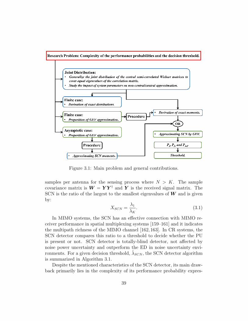
Figure 3.1: Main problem and general contributions.
samples per antenna for the sensing process where N > K. The samplecovariance matrix is W = Y Y † and Y is the received signal matrix. TheSCN is the ratio of the largest to the smallest eigenvalues of W and is givenby:
XSCN =λ1
λK. (3.1)
In MIMO systems, the SCN has an effective connection with MIMO re-ceiver performance in spatial multiplexing systems [159–161] and it indicatesthe multipath richness of the MIMO channel [162, 163]. In CR systems, theSCN detector compares this ratio to a threshold to decide whether the PUis present or not. SCN detector is totally-blind detector, not affected bynoise power uncertainty and outperform the ED in noise uncertainty envi-ronments. For a given decision threshold, λSCN , the SCN detector algorithmis summarized in Algorithm 3.1.
Despite the mentioned characteristics of the SCN detector, its main draw-back primarily lies in the complexity of its performance probability expres-
39
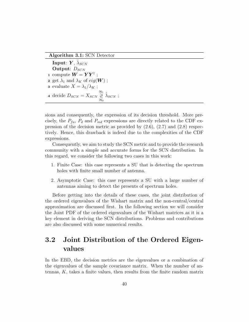
Algorithm 3.1: SCN Detector
Input: Y , λSCNOutput: DSCN
1 compute W = Y Y † ;2 get λ1 and λK of eig(W ) ;3 evaluate X = λ1/λK ;
4 decide DSCN = XSCN
H1
≷H0
λSCN ;
sions and consequently, the expression of its decision threshold. More pre-cisely, the Pfa, Pd and Pmd expressions are directly related to the CDF ex-pression of the decision metric as provided by (2.6), (2.7) and (2.8) respec-tively. Hence, this drawback is indeed due to the complexities of the CDFexpressions.
Consequently, we aim to study the SCN metric and to provide the researchcommunity with a simple and accurate forms for the SCN distribution. Inthis regard, we consider the following two cases in this work:
1. Finite Case: this case represents a SU that is detecting the spectrumholes with finite small number of antenna.
2. Asymptotic Case: this case represents a SU with a large number ofantennas aiming to detect the presents of spectrum holes.
Before getting into the details of these cases, the joint distribution ofthe ordered eigenvalues of the Wishart matrix and the non-central/centralapproximation are discussed first. In the following section we will considerthe Joint PDF of the ordered eigenvalues of the Wishart matrices as it is akey element in deriving the SCN distributions. Problems and contributionsare also discussed with some numerical results.
3.2 Joint Distribution of the Ordered Eigen-
values
In the EBD, the decision metrics are the eigenvalues or a combination ofthe eigenvalues of the sample covariance matrix. When the number of an-tennas, K, takes a finite values, then results from the finite random matrix
40
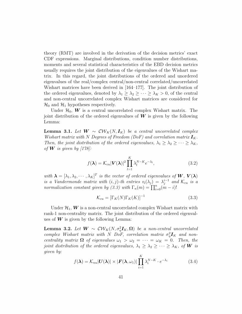
theory (RMT) are involved in the derivation of the decision metrics’ exactCDF expressions. Marginal distributions, condition number distributions,moments and several statistical characteristics of the EBD decision metricsusually requires the joint distribution of the eigenvalues of the Wishart ma-trix. In this regard, the joint distributions of the ordered and unorderedeigenvalues of the real/complex central/non-central correlated/uncorrelatedWishart matrices have been derived in [164–177]. The joint distribution ofthe ordered eigenvalues, denoted by λ1 ≥ λ2 ≥ · · · ≥ λK > 0, of the centraland non-central uncorrelated complex Wishart matrices are considered forH0 and H1 hypotheses respectively.
Under H0, W is a central uncorrelated complex Wishart matrix. Thejoint distribution of the ordered eigenvalues of W is given by the followingLemma:
Lemma 3.1. Let W ∼ CWK(N, IK) be a central uncorrelated complexWishart matrix with N Degrees of Freedom (DoF) and correlation matrix IK.Then, the joint distribution of the ordered eigenvalues, λ1 ≥ λ2 ≥ · · · ≥ λK,of W is given by [178]:
f(λ) = Kcu|V (λ)|2K∏l=1
λN−Kl e−λl , (3.2)
with λ = [λ1, λ2, · · · , λK ]T is the vector of ordered eigenvalues of W , V (λ)is a Vandermonde matrix with (i, j)-th entries vi(λj) = λi−1
j and Kcu is anormalization constant given by (3.3) with Γn(m) =
∏ni=0(m− i)!
Kcu = [ΓK(N)ΓK(K)]−1 (3.3)
Under H1, W is a non-central uncorrelated complex Wishart matrix withrank-1 non-centrality matrix. The joint distribution of the ordered eigenval-ues of W is given by the following Lemma:
Lemma 3.2. Let W ∼ CWK(N, σ2ηIK ,Ω) be a non-central uncorrelated
complex Wishart matrix with N DoF, correlation matrix σ2ηIK and non-
centrality matrix Ω of eigenvalues ω1 > ω2 = · · · = ωK = 0. Then, thejoint distribution of the ordered eigenvalues, λ1 ≥ λ2 ≥ · · · ≥ λK, of W isgiven by:
f(λ) = Knu|U(λ)| × |F (λ, ω1)|K∏i=1
λN−Ki · e−λi (3.4)
41
where U(λ) and F (λ, ω1) are K ×K matrices of (i, j)-th entries given re-spectively by ui(λj) = λK−ij and (3.5). In (3.5), 0F1(., .) is the generalizedhypergeometric function defined in [179, Eq. 9.14.1]. Knu is defined in (3.6).
fi(λj) =
0F1(N −K + 1, ω1λj) i = 1λK−ij ·(N−K)!
(N−i)! i = 2, · · · , K(3.5)
Knu =e−ω1 · [(N −K)!]−K
ΓK−1(K − 1) · ωK−11
(3.6)
Proof. Particularize [180, App. I] with Ω is a rank-1 matrix.
Under H1 hypothesis, one can sometimes obtain explicit solutions for thedistributional properties of the non-central Wishart matrices. However, theseexpressions are usually more complicated than that of the central Wishartmatrices. For example, the exact general form of the distribution of SCNof the non-central uncorrelated complex Wishart matrix with full rank non-centrality matrix is derived in [157], however, further numerical evaluationwould either require Nuttall-Q function which could be replaced by Mar-cum Q-function and a finite weighted sum of Bessel functions [181] or byhypergeometric functions that could be expanded to an infinite sum (See, forexample, [182] for K = 2 and N = 2) [157]. In this regard, using certainmethod that approximates a non-central Wishart distribution by a centralWishart distribution would be practical. In this light, consider the followingLemma that approximate the non-central Wishart distribution with a centralWishart distribution by modifying its correlation matrix.
Lemma 3.3. [183] The non-central uncorrelated complex Wishart matrixW ∼ CWK(N, σ2
ηIK ,Ω) and the central semi-correlated complex Wishart
matrix W ∼ CWK(N, Σ) with effective correlation matrix Σ = σ2ηIK + Ω/N
have the same first and second-order moments differing by Ω/N .
Yet, Lemma 3.3 was used in the approximation of several marginal dis-tributions and condition numbers such as the LE, SCN and DCN where theRicean fading MIMO channel matrix has been studied [157,184]. It has beenreported that the accuracy of this approximation deteriorates at high RiceanK-factors [157]. From SS perspective, this approximation has been also usedto replace the CDF of the SCN of the dual non-central Wishart matrices by
42
that of the dual central Wishart matrices under H1 hypothesis [44]. How-ever, the impact of CR system parameters, such as the SNR, N and K, onthe accuracy of this approximation for Pd or Pmd has not been studied.
Moreover, work done on the joint distribution of the ordered eigenval-ues of the central semi-correlated Wishart matrices has considered that theeigenvalues of the correlation matrix, Σ, are all distinct [157]. Indeed, theseeigenvalues may coincide as the case in SS. Recall that under H1 hypothesisthe non-centrality matrix, Ω, is a rank-1 matrix where the nonzero eigenvalueis denoted by ω1 and is given by:
ω1 = NKρ. (3.7)
Consequently, the correlation matrix of the corresponding central semi-correlated Wishart matrix, due to Lemma 3.3, is given by:
Σ = σ2ηIK +
1
NΩ. (3.8)
Accordingly, all but one eigenvalue of the eigenvalues of Σ are equal to σ2η
while σ1, the remaining eigenvalue, is given by:
σ1 = σ2η +
ω1
N. (3.9)
Therefore, by considering the non-central/central approximation, resultsbased on assuming all the eigenvalues of the correlation matrix are distinctcould not be used. Next, we consider the joint distribution of the orderedeigenvalues of the central semi-correlated complex Wishart matrices wherethe correlation matrix have some coincide eigenvalues. Moreover, the im-pact of the SNR, K and N on the non-central/central approximation is alsostudied via simulations.
3.2.1 Central Semi-correlated Wishart Case
As mentioned, all but one of the eigenvalues of the correlation matrix areequal. In this section, we generalize the joint distribution of the orderedeigenvalues of the central semi-correlated Wishart matrix. This new formconsiders any number L of equal eigenvalues positioned anywhere in vectorof eigenvalues of the correlation matrix σ and is given in Theorem 3.1 below.
43

Theorem 3.1. Let W be a central semi-correlated complex Wishart matrixW ∼ CWK(N,Σ), and denote by σ1 > σ2 > · · · > σp = · · · = σq >· · · > σK > 0 the ordered eigenvalues of Σ assumed full rank with L equaleigenvalues (from p to q with q = p+ L− 1), then the joint PDF of λ couldbe written as:
f(λ) = Kcc1|V (λ)| × |E(λ,σ)|K∏i=1
λN−Ki , (3.10)
where Kcc1 is a normalization constant given by:
Kcc1 =
∏Ki<j σiσj
K∏i=1
(N − i)!σNiK∏i<jσi 6=σj
(σj − σi) ΓL(L)
, (3.11)
and E(λ,σ) is a K ×K matrix with (i, j)-th entry:
E(λ,σ)i,j =
∂q−i(e
−λjσp )
∂σq−ipp ≤ i ≤ q
e−λjσi otherwise
, (3.12)
where the n-th partial derivative in (3.12) is given by (3.13) and the Lahnumber is defined by L(n, k) =
(nk
)(n−1k−1
)(n− k)!.
∂n(e−λjσp )
∂σnp=
e−λjσp
n∑k=1
(−1)k+n·L(n,k)·λkjσn+kp
if n > 0
e−λjσp if n = 0
(3.13)
Proof. See Appendix A.1.
It can be easily shown that by taking L = 1, the parameters in theorem 3.1will be equivalent to the case of all distinct eigenvalues in the literature [157,Table I].
3.2.2 Numerical Results and Discussion
In this section, we discuss the analytical results through Monte-Carlo sim-ulations. We, firstly, validate the theoretical analysis presented in Theorem
44
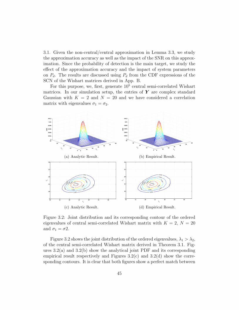
3.1. Given the non-central/central approximation in Lemma 3.3, we studythe approximation accuracy as well as the impact of the SNR on this approx-imation. Since the probability of detection is the main target, we study theeffect of the approximation accuracy and the impact of system parameterson Pd. The results are discussed using Pd from the CDF expressions of theSCN of the Wishart matrices derived in App. B.
For this purpose, we, first, generate 105 central semi-correlated Wishartmatrices. In our simulation setup, the entries of Y are complex standardGaussian with K = 2 and N = 20 and we have considered a correlationmatrix with eigenvalues σ1 = σ2.
010
2030
4050
60
0
10
20
30
400
0.002
0.004
0.006
0.008
0.01
0.012
λ1
λ2
PD
F
(a) Analytic Result.
010
2030
4050
60
0
10
20
30
400
0.002
0.004
0.006
0.008
0.01
0.012
λ1
λ2
PD
F
(b) Empirical Result.
0.00
2
0.002
0.00
2
0.002
0.00
4
0.004
0.004
0.004
0.00
6
0.006
0.006
0.00
8
0.00
8
0.01
0.01
0.012
λ1
λ 2
10 15 20 25 30 35 405
10
15
20
25
30
(c) Analytic Result.
0.00
2
0.002
0.00
2
0.002
0.00
4
0.004
0.004
0.004
0.00
6
0.006
0.006
0.008
0.00
8
0.01
0.01
0.012
λ1
λ 2
10 15 20 25 30 35 405
10
15
20
25
30
(d) Empirical Result.
Figure 3.2: Joint distribution and its corresponding contour of the orderedeigenvalues of central semi-correlated Wishart matrix with K = 2, N = 20and σ1 = σ2.
Figure 3.2 shows the joint distribution of the ordered eigenvalues, λ1 > λ2,of the central semi-correlated Wishart matrix derived in Theorem 3.1. Fig-ures 3.2(a) and 3.2(b) show the analytical joint PDF and its correspondingempirical result respectively and Figures 3.2(c) and 3.2(d) show the corre-sponding contours. It is clear that both figures show a perfect match between
45
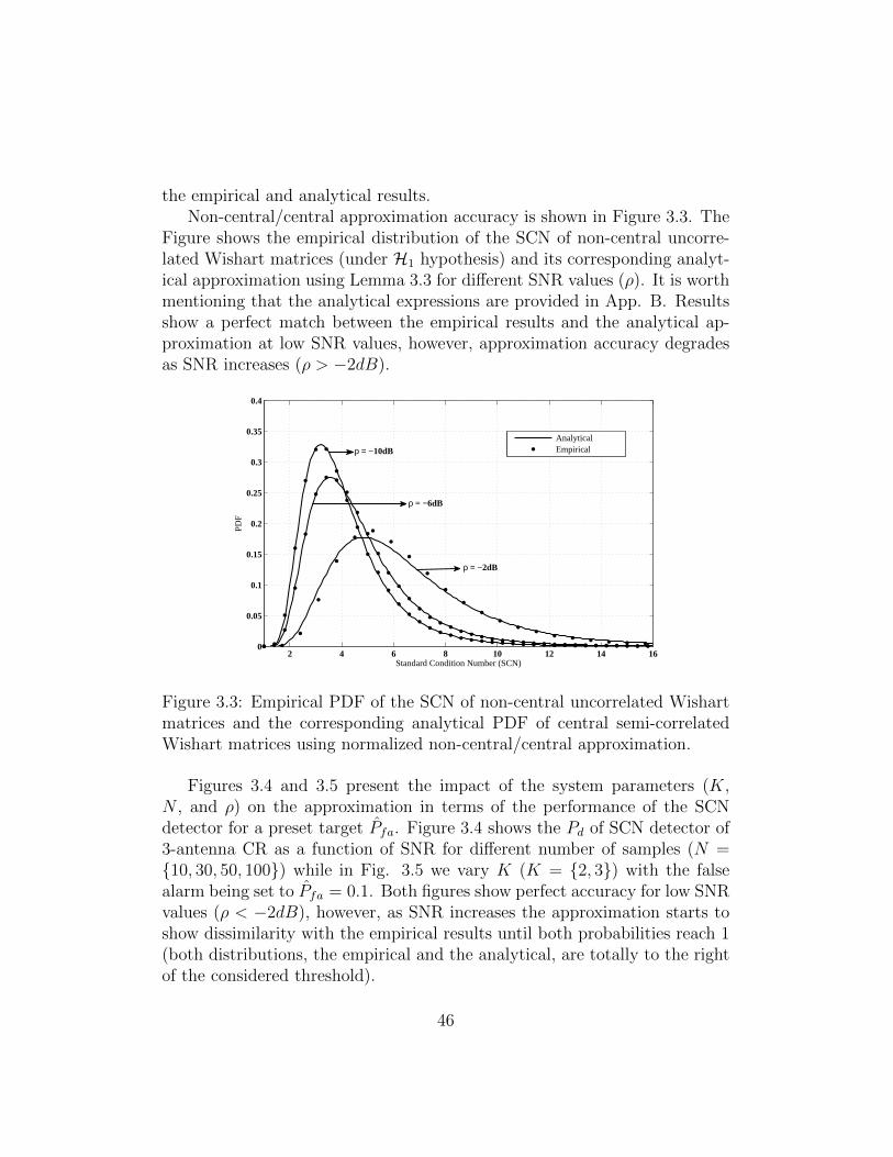
the empirical and analytical results.Non-central/central approximation accuracy is shown in Figure 3.3. The
Figure shows the empirical distribution of the SCN of non-central uncorre-lated Wishart matrices (under H1 hypothesis) and its corresponding analyt-ical approximation using Lemma 3.3 for different SNR values (ρ). It is worthmentioning that the analytical expressions are provided in App. B. Resultsshow a perfect match between the empirical results and the analytical ap-proximation at low SNR values, however, approximation accuracy degradesas SNR increases (ρ > −2dB).
2 4 6 8 10 12 14 160
0.05
0.1
0.15
0.2
0.25
0.3
0.35
0.4
Standard Condition Number (SCN)
AnalyticalEmpiricalρ = −10dB
ρ = −6dB
ρ = −2dB
Figure 3.3: Empirical PDF of the SCN of non-central uncorrelated Wishartmatrices and the corresponding analytical PDF of central semi-correlatedWishart matrices using normalized non-central/central approximation.
Figures 3.4 and 3.5 present the impact of the system parameters (K,N , and ρ) on the approximation in terms of the performance of the SCNdetector for a preset target Pfa. Figure 3.4 shows the Pd of SCN detector of3-antenna CR as a function of SNR for different number of samples (N =10, 30, 50, 100) while in Fig. 3.5 we vary K (K = 2, 3) with the falsealarm being set to Pfa = 0.1. Both figures show perfect accuracy for low SNRvalues (ρ < −2dB), however, as SNR increases the approximation starts toshow dissimilarity with the empirical results until both probabilities reach 1(both distributions, the empirical and the analytical, are totally to the rightof the considered threshold).
46
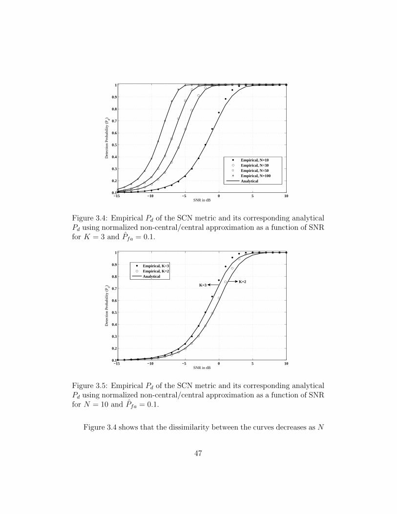
−15 −10 −5 0 5 100.1
0.2
0.3
0.4
0.5
0.6
0.7
0.8
0.9
1
SNR in dB
Det
ectio
n Pr
obab
ility
(P d)
Empirical, N=10Empirical, N=30Empirical, N=50Empirical, N=100Analytical
Figure 3.4: Empirical Pd of the SCN metric and its corresponding analyticalPd using normalized non-central/central approximation as a function of SNRfor K = 3 and Pfa = 0.1.
−15 −10 −5 0 5 100.1
0.2
0.3
0.4
0.5
0.6
0.7
0.8
0.9
1
SNR in dB
Det
ectio
n Pr
obab
ility
(P d)
Empirical, K=3Empirical, K=2Analytical
K=2K=3
Figure 3.5: Empirical Pd of the SCN metric and its corresponding analyticalPd using normalized non-central/central approximation as a function of SNRfor N = 10 and Pfa = 0.1.
Figure 3.4 shows that the dissimilarity between the curves decreases as N
47
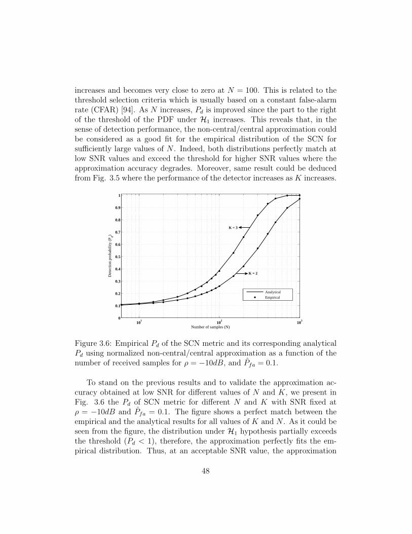
increases and becomes very close to zero at N = 100. This is related to thethreshold selection criteria which is usually based on a constant false-alarmrate (CFAR) [94]. As N increases, Pd is improved since the part to the rightof the threshold of the PDF under H1 increases. This reveals that, in thesense of detection performance, the non-central/central approximation couldbe considered as a good fit for the empirical distribution of the SCN forsufficiently large values of N . Indeed, both distributions perfectly match atlow SNR values and exceed the threshold for higher SNR values where theapproximation accuracy degrades. Moreover, same result could be deducedfrom Fig. 3.5 where the performance of the detector increases as K increases.
101
102
103
0
0.1
0.2
0.3
0.4
0.5
0.6
0.7
0.8
0.9
1
Number of samples (N)
Det
ectio
n pr
obab
ility
(P d)
Analytical
Empirical
K = 2
K = 3
Figure 3.6: Empirical Pd of the SCN metric and its corresponding analyticalPd using normalized non-central/central approximation as a function of thenumber of received samples for ρ = −10dB, and Pfa = 0.1.
To stand on the previous results and to validate the approximation ac-curacy obtained at low SNR for different values of N and K, we present inFig. 3.6 the Pd of SCN metric for different N and K with SNR fixed atρ = −10dB and Pfa = 0.1. The figure shows a perfect match between theempirical and the analytical results for all values of K and N . As it could beseen from the figure, the distribution under H1 hypothesis partially exceedsthe threshold (Pd < 1), therefore, the approximation perfectly fits the em-pirical distribution. Thus, at an acceptable SNR value, the approximation
48
doesn’t show any degradation as N and K values change.
3.2.3 Section Conclusion
Through this section, we have considered the joint distribution of the or-dered eigenvalue of different Wishart matrices. Under H1 hypothesis, thenon-central/central approximation is considered as a practical solution toavoid the difficult manipulation and the complicated analytical results whenusing the non-central uncorrelated Wishart matrix statistical properties. Inthis regard, we have derived the expression of the joint PDF of the orderedeigenvalues of the central semi-correlated complex Wishart matrices when thecorrelation matrix exhibit equal eigenvalues. Based on these results, we studythe impact of system parameters on Pd when using the non-central/centralapproximation. Results have shown that this approximation has perfect ac-curacy for low SNR values and could be considered as a good fit for Pd forsufficiently large values of N when the SNR is high.
3.3 Finite Case
Herein, we consider the SCN detector in the finite case where K > 1 takessmall values. In literature, the authors in [157] provided the exact genericform of the distribution of the SCN based on the joint distribution of theordered eigenvalues of Wishart matrices. Consequently, [44] provides theexact forms of the Pfa of the SCN detector for CR with two antenna (i.e.dual case). In addition, the Pd for 2-dimensional systems was approximatedusing the non-central/central approximation and provided in [44] followingthe results in [157].
In this section, we first derive the exact distribution of the SCN metricusing the joint distributions provided by Sec. 3.2. A general nested form forthe CDF and the PDF of the SCN of the central uncorrelated, non-centraluncorrelated and central semi-correlated complex Wishart matrices are de-rived. Consequently, it could be easily deduced that lookup tables (LUT)must be constructed and used to avoid computational complexity. In thisregard, we provide an alternative solution as we propose a new approxima-tion for the SCN based on the generalized extreme value (GEV) distribution.For this purpose, we derive the exact form of the p-th moment of the SCNto match the first three moments of the GEV distribution. This approxi-
49
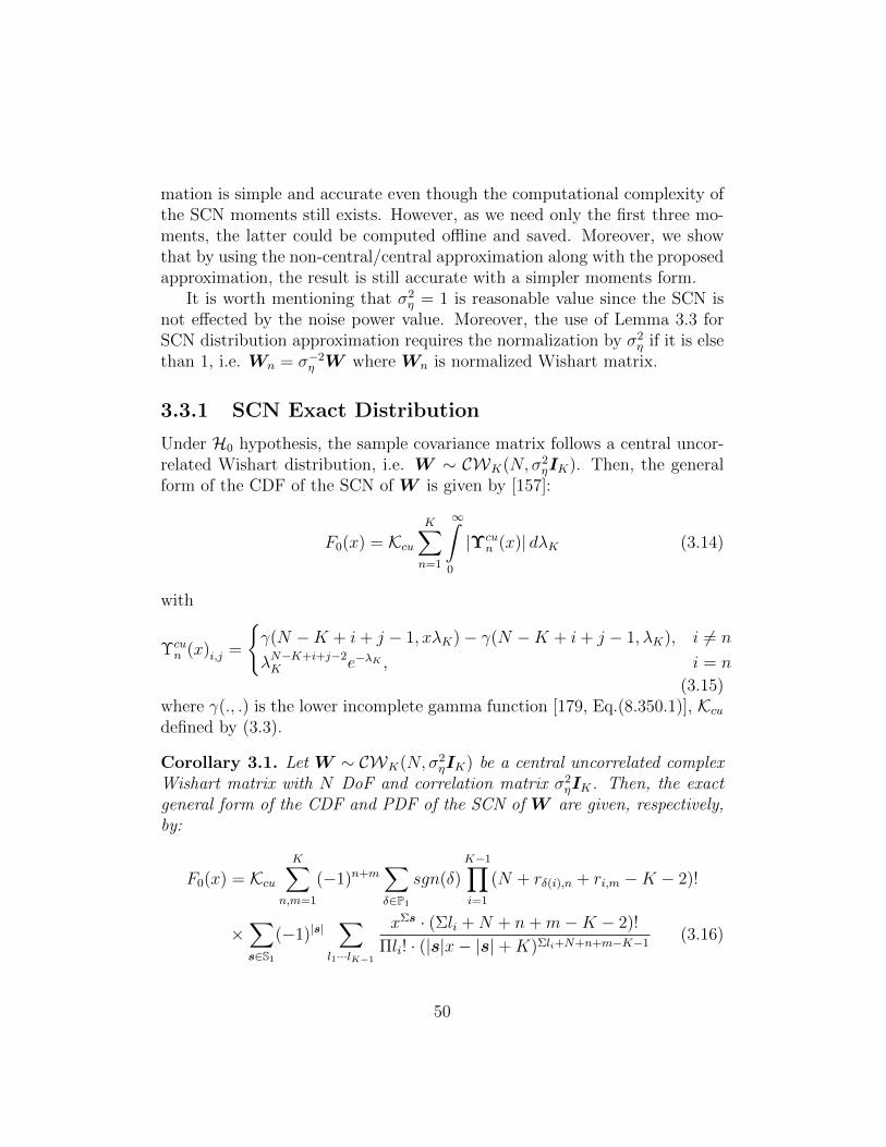
mation is simple and accurate even though the computational complexity ofthe SCN moments still exists. However, as we need only the first three mo-ments, the latter could be computed offline and saved. Moreover, we showthat by using the non-central/central approximation along with the proposedapproximation, the result is still accurate with a simpler moments form.
It is worth mentioning that σ2η = 1 is reasonable value since the SCN is
not effected by the noise power value. Moreover, the use of Lemma 3.3 forSCN distribution approximation requires the normalization by σ2
η if it is elsethan 1, i.e. Wn = σ−2
η W where Wn is normalized Wishart matrix.
3.3.1 SCN Exact Distribution
Under H0 hypothesis, the sample covariance matrix follows a central uncor-related Wishart distribution, i.e. W ∼ CWK(N, σ2
ηIK). Then, the generalform of the CDF of the SCN of W is given by [157]:
F0(x) = KcuK∑n=1
∞∫0
|Υcun (x)| dλK (3.14)
with
Υcun (x)i,j =
γ(N −K + i+ j − 1, xλK)− γ(N −K + i+ j − 1, λK), i 6= n
λN−K+i+j−2K e−λK , i = n
(3.15)where γ(., .) is the lower incomplete gamma function [179, Eq.(8.350.1)], Kcudefined by (3.3).
Corollary 3.1. Let W ∼ CWK(N, σ2ηIK) be a central uncorrelated complex
Wishart matrix with N DoF and correlation matrix σ2ηIK. Then, the exact
general form of the CDF and PDF of the SCN of W are given, respectively,by:
F0(x) = KcuK∑
n,m=1
(−1)n+m∑δ∈P1
sgn(δ)K−1∏i=1
(N + rδ(i),n + ri,m −K − 2)!
×∑s∈S1
(−1)|s|∑
l1···lK−1
xΣs · (Σli +N + n+m−K − 2)!
Πli! · (|s|x− |s|+K)Σli+N+n+m−K−1(3.16)
50
f0(x) = KcuK∑
n,m=1
(−1)n+m∑δ∈P1
sgn(δ)K−1∏i=1
(N + rδ(i),n + ri,m −K − 2)!∑s∈S1
(−1)|s|
×∑
l1···lK−1
xΣs[Σsx−1(|s|x− |s|+K)− |s|(Σli +N + n+m−K − 1)]
Πli! · [(Σli +N + n+m−K − 2)!]−1 · (|s|x− |s|+K)Σli+N+n+m−K
(3.17)
where P1 and S1 are, respectively, the set of all possible permutations andsubsets of the vector [1, · · · , K−1]. sgn(δ) is the permutation sign and |s| is
the cardinality.∑
l1···lK−1=∑L1
l1· · ·∑LK−1
lK−1with Lj = N+rδ(j),n+rj,m−K−2;
Σs, Σli and Πli! are, respectively, the sum of the values of li ∈ s, the sumof the values of l1≤i≤K−1 and the product of the factorial of the values ofl1≤i≤K−1. Finally, ri,j is defined as:
ri,j =
i i < j
i+ 1 i ≥ j(3.18)
Proof. Refer to Appendix A.2.
Under H1 hypothesis, the sample covariance matrix follows a non-centraluncorrelated Wishart distribution, W ∼ CWK(N, σ2
ηIK ,Ω), with rank-1non-centrality matrix Ω. Then, the exact generic form of the SCN CDFunder H1 hypothesis is given by the following Theorem:
Theorem 3.2. Let W ∼ CWK(N, σ2ηIK ,Ω) be a non-central uncorrelated
complex Wishart matrix with N DoF, correlation matrix σ2ηIK and non-
centrality matrix Ω of eigenvalues ω1 > ω2 = · · · = ωK = 0. Then, theCDF of the SCN of W is given by:
F1(x) = KnuK∑n=1
∞∫0
|Υnun (x)| dλK (3.19)
with
Υnun (x)i,j =
Inui,j =
xλK∫λK
fj(u)uN−ie−udu, i 6= n
fj(λK)λN−iK e−λK , i = n
(3.20)
51
where fj(.) is given in (3.5) and the integral in (3.20) has analytical solutiongiven by:
Inui,j =
∞∑l=0
ωl1(N−K+1)ll!
[γ(N − i+ l + 1, xλK)− γ(N − i+ l + 1, λK)
]j = 1
(N−K)!(N−j)!
[γ(N +K − i− j + 1, xλK)− γ(N +K − i− j + 1, λK)
]j = 2, · · · , K
(3.21)
Proof. Refer to Appendix A.3.
Corollary 3.2. Let W ∼ CWK(N, σ2ηIK ,Ω) be a non-central uncorrelated
complex Wishart matrix with N DoF, correlation matrix σ2ηIK and non-
centrality matrix Ω of eigenvalues ω1 > ω2 = · · · = ωK = 0. Then, theexact general form of the CDF and PDF of the SCN of W is given, respec-tively, by:
F1(x) = K′nuK∑
n,m=1
(−1)n+m
∞∑h=0
ωh1(N −K + h)!h!
∑δ∈P1
sgn(δ)K−1∏i=1
(N − rδ(i),n + gri,m,1(h,K))!
×∑s∈S1
(−1)|s|∑
l1···lK−1
xΣs · (Σli +N − n+ gm,1(h,K))!
Πli! · (|s|x− |s|+K)Σli+N−n+gm,1(h,K)+1(3.22)
f1(x) = K′nuK∑
n,m=1
(−1)n+m
∞∑h=0
ωh1(N −K + h)!h!
∑δ∈P1
sgn(δ)K−1∏i=1
(N − rδ(i),n + gri,m,1(h,K))!
×∑s∈S1
(−1)|s|∑
l1···lK−1
xΣs[Σsx−1(|s|x− |s|+K)− |s|(Σli +N − n+ gm,1(h,K) + 1)]
Πli! · [(Σli +N − n+ gm,1(h,K))!]−1 · (|s|x− |s|+K)Σli+N−n+gm,1(h,K)+2
(3.23)
with
K′nu =
[ΓK−1(K − 1)
K∏i=2
(N − i)!ωK−11 eω1
]−1
, (3.24)
and∑
l1···lK−1=∑L1
l1· · ·∑LK−1
lK−1with Lj = N − rδ(j),n + grj,m,1(h,K) and we
define gi,j(a, b) as:
gi,j(a, b) =
a i = j
b− i i 6= j(3.25)
52
Proof. Refer to Appendix A.2.
Under H1 hypothesis and using Lemma 3.1, the sample covariance matrixcould be approximated by a central semi-correlated Wishart distribution,W ∼ CWK(N,Σ), with correlation matrix having K − 1 equal eigenvalues.The exact generic form of the SCN CDF for the H1 hypothesis is given bythe following Theorem:
Theorem 3.3. Let W ∼ CWK(N,Σ) be a Central Semi-Correlated Wishartmatrix with N DoF and correlation matrix Σ of eigenvalues σ1 > σ2 = · · · =σK. Then, the CDF of the SCN of W is given by:
F1(x) = KccK∑n=1
∞∫0
|Υccn (x)| dλK (3.26)
with
Υccn (x)i,j =
Icci,j =
xλK∫λK
ej(u)uN+i−K−1du, i 6= n
ej(λK)λN+i−K−1K , i = n
(3.27)
where ej(.) is given in (A.6) and the integral in (3.27) has an analyticalsolution given by:
Icci,j =
[γ(N + i−K, xλK
σ1)− γ(N + i−K, λK
σ1)]· σN+i−K
1 j = 1
(−1)K−j[γ(N + i− j, xλK
σ2)− γ(N + i− j, λK
σ2)]σN+i−j
2 j = 2, · · · , K(3.28)
Proof. Refer to Appendix A.3.
Corollary 3.3. Let W ∼ CWK(N,Σ) be a Central Semi-Correlated Wishartmatrix with N DoF and correlation matrix Σ of eigenvalues σ1 > σ2 = · · · =σK. Then, the exact general form of the CDF and PDF of the SCN of W isgiven, respectively, by:
F1(x) = K′ccK∑
n,m=1
(−1)n+m∑δ∈P1
sgn(δ)K−1∏i=1
(N + rδ(i),n − gri,m,1(K, 2i)− 1)!
σ−(N+rδ(i),n−gri,m,1(K,2i))ri,m
×∑s∈S1
(−1)|s|∑
l1···lK−1
xΣs · (Σli +N + n− gm,1(K, 2i)− 1)!
Πli! · Πσliri,m · (Σs xσsi,m
+ Σs1
σsi,m+ 1
σm)Σli+N+n−gm,1(K,2i)
(3.29)
53
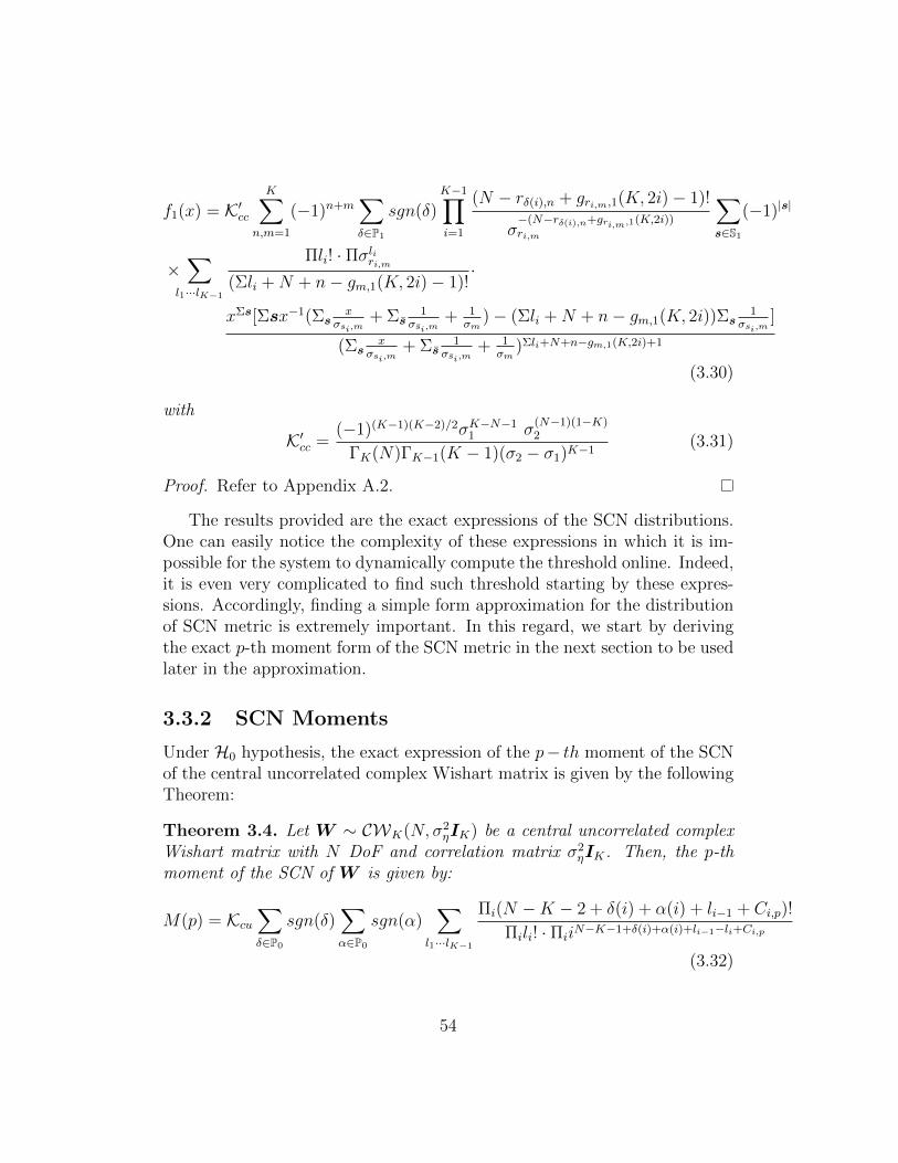
f1(x) = K′ccK∑
n,m=1
(−1)n+m∑δ∈P1
sgn(δ)K−1∏i=1
(N − rδ(i),n + gri,m,1(K, 2i)− 1)!
σ−(N−rδ(i),n+gri,m,1(K,2i))ri,m
∑s∈S1
(−1)|s|
×∑
l1···lK−1
Πli! · Πσliri,m(Σli +N + n− gm,1(K, 2i)− 1)!
·
xΣs[Σsx−1(Σsx
σsi,m+ Σs
1σsi,m
+ 1σm
)− (Σli +N + n− gm,1(K, 2i))Σs1
σsi,m]
(Σsx
σsi,m+ Σs
1σsi,m
+ 1σm
)Σli+N+n−gm,1(K,2i)+1
(3.30)
with
K′cc =(−1)(K−1)(K−2)/2σK−N−1
1 σ(N−1)(1−K)2
ΓK(N)ΓK−1(K − 1)(σ2 − σ1)K−1(3.31)
Proof. Refer to Appendix A.2.
The results provided are the exact expressions of the SCN distributions.One can easily notice the complexity of these expressions in which it is im-possible for the system to dynamically compute the threshold online. Indeed,it is even very complicated to find such threshold starting by these expres-sions. Accordingly, finding a simple form approximation for the distributionof SCN metric is extremely important. In this regard, we start by derivingthe exact p-th moment form of the SCN metric in the next section to be usedlater in the approximation.
3.3.2 SCN Moments
Under H0 hypothesis, the exact expression of the p− th moment of the SCNof the central uncorrelated complex Wishart matrix is given by the followingTheorem:
Theorem 3.4. Let W ∼ CWK(N, σ2ηIK) be a central uncorrelated complex
Wishart matrix with N DoF and correlation matrix σ2ηIK. Then, the p-th
moment of the SCN of W is given by:
M(p) = Kcu∑δ∈P0
sgn(δ)∑α∈P0
sgn(α)∑
l1···lK−1
Πi(N −K − 2 + δ(i) + α(i) + li−1 + Ci,p)!
Πili! · ΠiiN−K−1+δ(i)+α(i)+li−1−li+Ci,p
(3.32)
54
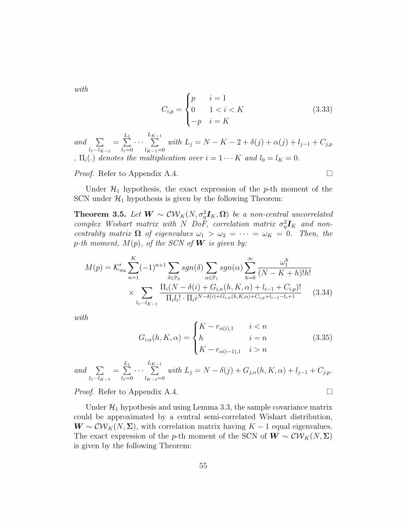
with
Ci,p =
p i = 1
0 1 < i < K
−p i = K
(3.33)
and∑
l1···lK−1
=L1∑l1=0
· · ·LK−1∑lK−1=0
with Lj = N −K − 2 + δ(j) + α(j) + lj−1 + Cj,p
, Πi(.) denotes the multiplication over i = 1 · · ·K and l0 = lK = 0.
Proof. Refer to Appendix A.4.
Under H1 hypothesis, the exact expression of the p-th moment of theSCN under H1 hypothesis is given by the following Theorem:
Theorem 3.5. Let W ∼ CWK(N, σ2ηIK ,Ω) be a non-central uncorrelated
complex Wishart matrix with N DoF, correlation matrix σ2ηIK and non-
centrality matrix Ω of eigenvalues ω1 > ω2 = · · · = ωK = 0. Then, thep-th moment, M(p), of the SCN of W is given by:
M(p) = K′nuK∑n=1
(−1)n+1∑δ∈P0
sgn(δ)∑α∈P1
sgn(α)∞∑h=0
ωh1(N −K + h)!h!
×∑
l1···lK−1
Πi(N − δ(i) +Gi,n(h,K, α) + li−1 + Ci,p)!
Πili! · ΠiiN−δ(i)+Gi,n(h,K,α)+Ci,p+li−1−li+1(3.34)
with
Gi,n(h,K, α) =
K − rα(i),1 i < n
h i = n
K − rα(i−1),1 i > n
(3.35)
and∑
l1···lK−1
=L1∑l1=0
· · ·LK−1∑lK−1=0
with Lj = N − δ(j) +Gj,n(h,K, α) + lj−1 + Cj,p.
Proof. Refer to Appendix A.4.
Under H1 hypothesis and using Lemma 3.3, the sample covariance matrixcould be approximated by a central semi-correlated Wishart distribution,W ∼ CWK(N,Σ), with correlation matrix having K − 1 equal eigenvalues.The exact expression of the p-th moment of the SCN of W ∼ CWK(N,Σ)is given by the following Theorem:
55
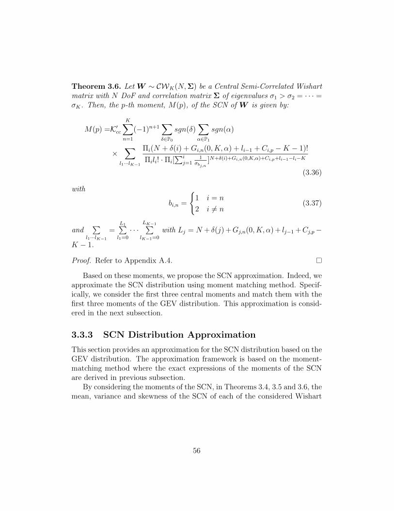
Theorem 3.6. Let W ∼ CWK(N,Σ) be a Central Semi-Correlated Wishartmatrix with N DoF and correlation matrix Σ of eigenvalues σ1 > σ2 = · · · =σK. Then, the p-th moment, M(p), of the SCN of W is given by:
M(p) =K′ccK∑n=1
(−1)n+1∑δ∈P0
sgn(δ)∑α∈P1
sgn(α)
×∑
l1···lK−1
Πi(N + δ(i) +Gi,n(0, K, α) + li−1 + Ci,p −K − 1)!
Πili! · Πi[∑i
j=11
σbj,n]N+δ(i)+Gi,n(0,K,α)+Ci,p+li−1−li−K
(3.36)
with
bi,n =
1 i = n
2 i 6= n(3.37)
and∑
l1···lK−1
=L1∑l1=0
· · ·LK−1∑lK−1=0
with Lj = N + δ(j) +Gj,n(0, K, α) + lj−1 +Cj,p−
K − 1.
Proof. Refer to Appendix A.4.
Based on these moments, we propose the SCN approximation. Indeed, weapproximate the SCN distribution using moment matching method. Specif-ically, we consider the first three central moments and match them with thefirst three moments of the GEV distribution. This approximation is consid-ered in the next subsection.
3.3.3 SCN Distribution Approximation
This section provides an approximation for the SCN distribution based on theGEV distribution. The approximation framework is based on the moment-matching method where the exact expressions of the moments of the SCNare derived in previous subsection.
By considering the moments of the SCN, in Theorems 3.4, 3.5 and 3.6, themean, variance and skewness of the SCN of each of the considered Wishart
56
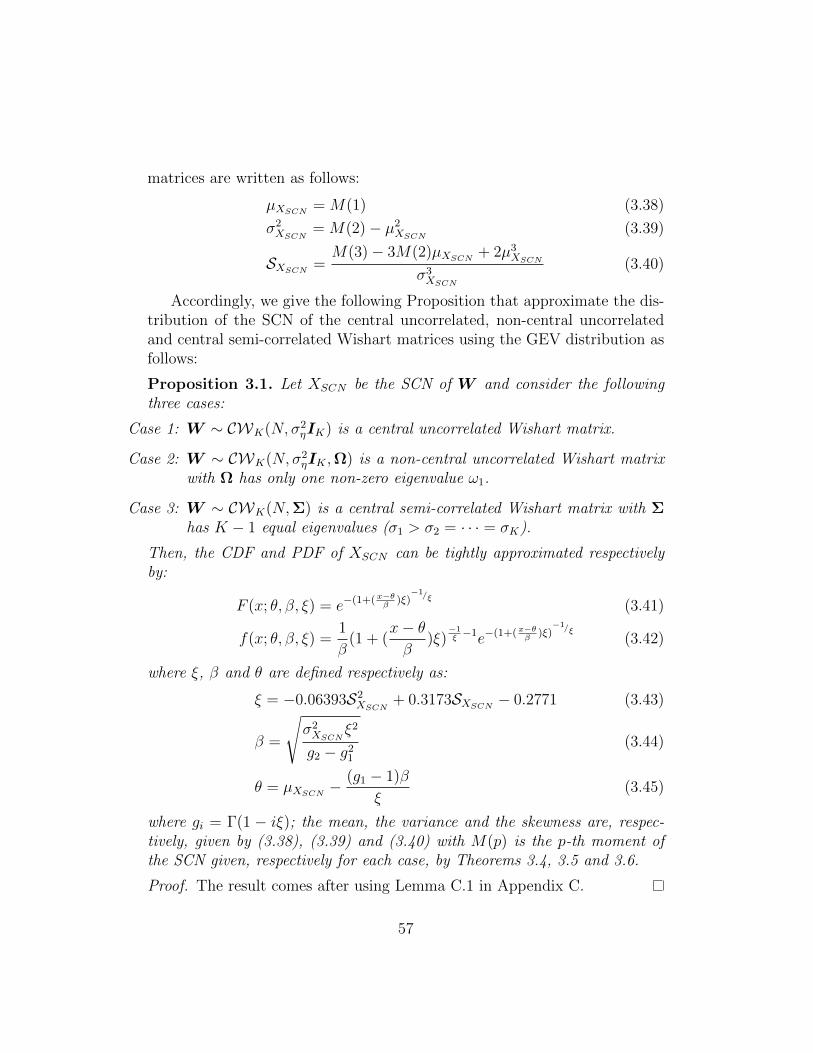
matrices are written as follows:
µXSCN = M(1) (3.38)
σ2XSCN
= M(2)− µ2XSCN
(3.39)
SXSCN =M(3)− 3M(2)µXSCN + 2µ3
XSCN
σ3XSCN
(3.40)
Accordingly, we give the following Proposition that approximate the dis-tribution of the SCN of the central uncorrelated, non-central uncorrelatedand central semi-correlated Wishart matrices using the GEV distribution asfollows:
Proposition 3.1. Let XSCN be the SCN of W and consider the followingthree cases:
Case 1: W ∼ CWK(N, σ2ηIK) is a central uncorrelated Wishart matrix.
Case 2: W ∼ CWK(N, σ2ηIK ,Ω) is a non-central uncorrelated Wishart matrix
with Ω has only one non-zero eigenvalue ω1.
Case 3: W ∼ CWK(N,Σ) is a central semi-correlated Wishart matrix with Σhas K − 1 equal eigenvalues (σ1 > σ2 = · · · = σK).
Then, the CDF and PDF of XSCN can be tightly approximated respectivelyby:
F (x; θ, β, ξ) = e−(1+(x−θβ
)ξ)−1/ξ
(3.41)
f(x; θ, β, ξ) =1
β(1 + (
x− θβ
)ξ)−1ξ−1e−(1+(x−θ
β)ξ)−1/ξ
(3.42)
where ξ, β and θ are defined respectively as:
ξ = −0.06393S2XSCN
+ 0.3173SXSCN − 0.2771 (3.43)
β =
√σ2XSCN
ξ2
g2 − g21
(3.44)
θ = µXSCN −(g1 − 1)β
ξ(3.45)
where gi = Γ(1 − iξ); the mean, the variance and the skewness are, respec-tively, given by (3.38), (3.39) and (3.40) with M(p) is the p-th moment ofthe SCN given, respectively for each case, by Theorems 3.4, 3.5 and 3.6.
Proof. The result comes after using Lemma C.1 in Appendix C.
57
3.3.4 Performance Probabilities and Decision Thresh-old
According to cases 1 and 2 of Proposition 3.1 and using (2.6), (2.7) and (2.8),then Pfa, Pd and Pmd are, respectively, given by:
Pfa = 1− e−(1+(λSCN−θ0
β0)ξ0)−1/ξ0
(3.46)
Pmd = 1− Pd = e−(1+(
λSCN−θ1β1
)ξ1)−1/ξ1
(3.47)
where ξ0, β0 and θ0 are the shape, scale and location parameters respec-tively under H0 hypothesis and are evaluated using (3.43), (3.44) and (3.45)respectively by considering the moments in Theorem 3.4; ξ1, β1 and θ1 arethe shape, scale and location parameters respectively under H1 hypothesisand are evaluated using (3.43), (3.44) and (3.45) respectively by consideringthe moments in Theorem 3.5.
An alternative approximation could be provided for Pmd and Pd usingboth Lemma 3.3 and case 3 of Proposition 3.1 which we refer to by the2-step approximation. In this approach, we first approximate the SCN ofthe non-central uncorrelated Wishart matrix by the SCN of central semi-correlated Wishart matrix due to Lemma 3.3 and then we approximate thelater using GEV approximation. Then, Pmd and Pd is still given by (3.47);however, the moments used in calculating θ1, β1 and ξ1 are given by Theorem3.6.
Accordingly, the threshold could be calculated. For example, for a CFAR,the threshold is given by:
λSCN = θ0 +β0
ξ0
(− 1 +
[− ln(1− Pfa)
]−ξ0) (3.48)
3.3.5 Comments on the Complexity
In practice, channel conditions are not stable and K and N may frequentlychange. Consequently, the implementation of the decision threshold must bedynamic and may rely on real-time computations rather than using LUTs.
The real-time computations are satisfied using the proposed thresholdin (3.48). However, the complexity still exists in the computation of theGEV parameters due to the complexity of the exact SCN moments. Thiscomplexity could be avoided by an offline computations of these parameters.
58
As a comparison; the exact SCN distribution needs a 1-D LUT for every(K,N) value under H0 hypothesis whereas only three values are needed inthe proposed GEV approximation (i.e. the 3 parameters). Further step isto approximate the SCN central moments using a simple formulation, andthus no need for the offline computation. This approach is provided in theAsymptotic case section.
3.3.6 Numerical Results and Discussion
In this section, the analytical results provided by Sections 3.3.1, 3.3.2, 3.3.3and 3.3.4 are discussed and validated through Monte-Carlo simulations. Thesimulation results are obtained by generating 105 random realizations of Y .To validate the results of central semi-correlated Wishart matrices, we haveconsidered a correlated complex Gaussian noise with zero mean and correla-tion matrix as defined in Lemma 3.3.
Figure 3.7 validates the analytical form of the distribution of the SCN ofthe three considered Wishart cases derived in Section 3.3.1. Figures 3.7(a),3.7(b) and 3.7(c) plot the empirical CDF of the SCN of central uncorrelated,non-central uncorrelated and central semi-correlated complex Wishart ma-trices respectively with the corresponding analytical form given by Theorems3.2 and 3.3 and by Corollaries 3.1, 3.2 and 3.3. The simulations are given fordifferent number of antennas (K = 2, 3, 4), N = 10 and SNR = −10dB.Results show a perfect match between the empirical SCN distribution andthe corresponding analytical form in each case.
Table 3.3.6 validates the analytical expressions of the p-th moment ofthe SCN of the central uncorrelated, non-central uncorrelated and centralsemi-correlated Wishart matrices provided in Theorems 3.4, 3.5 and 3.6 byconsidering the first moment. The SNR value is set to −10dB. Table 3.3.6shows a perfect accuracy in the analytical representation in each case. More-over, from the table and Figures 3.7(b) and 3.7(c), results also show a highaccuracy in the non-central/central approximation presented in Lemma 3.3.
Figure 3.8 shows the accuracy of the GEV approximation of the SCN ofthe three considered Wishart cases in Proposition 3.1. Figures 3.8(a), 3.8(b)and 3.8(c) plot the empirical CDF of the SCN and its corresponding GEVapproximations for different number of antennas (K = 2, 3, 4), N = 10 andSNR = −10dB. The results show high accuracy in the GEV approximationin all cases for different number of sensors.
The performance of the cognitive radio system is considered in Figures
59
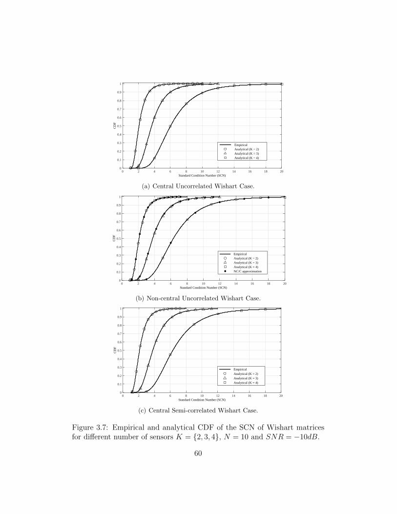
Standard Condition Number (SCN)0 2 4 6 8 10 12 14 16 18 20
CD
F
0
0.1
0.2
0.3
0.4
0.5
0.6
0.7
0.8
0.9
1
Empirical Analytical (K = 2) Analytical (K = 3) Analytical (K = 4)
(a) Central Uncorrelated Wishart Case.
Standard Condition Number (SCN)0 2 4 6 8 10 12 14 16 18 20
CD
F
0
0.1
0.2
0.3
0.4
0.5
0.6
0.7
0.8
0.9
1
Empirical Analytical (K = 2) Analytical (K = 3) Analytical (K = 4) NC/C approximation
(b) Non-central Uncorrelated Wishart Case.
Standard Condition Number (SCN)0 2 4 6 8 10 12 14 16 18 20
CD
F
0
0.1
0.2
0.3
0.4
0.5
0.6
0.7
0.8
0.9
1
Empirical Analytical (K = 2) Analytical (K = 3) Analytical (K = 4)
(c) Central Semi-correlated Wishart Case.
Figure 3.7: Empirical and analytical CDF of the SCN of Wishart matricesfor different number of sensors K = 2, 3, 4, N = 10 and SNR = −10dB.
60
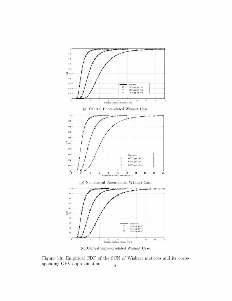
Standard Condition Number (SCN)0 2 4 6 8 10 12 14 16 18 20
CD
F
0
0.1
0.2
0.3
0.4
0.5
0.6
0.7
0.8
0.9
1
Empirical GEV app. (K = 2) GEV app. (K = 3) GEV app. (K = 4)
(a) Central Uncorrelated Wishart Case.
0 2 4 6 8 10 12 14 16 18 200
0.1
0.2
0.3
0.4
0.5
0.6
0.7
0.8
0.9
1
Standard Condition Number (SCN)
CD
F
Empirical
GEV app. (K=2)
GEV app. (K=3)
GEV app. (K=4)
(b) Non-central Uncorrelated Wishart Case.
Standard Condition Number (SCN)0 2 4 6 8 10 12 14 16 18 20
CD
F
0
0.1
0.2
0.3
0.4
0.5
0.6
0.7
0.8
0.9
1
Empirical GEV app. (K=2) GEV app. (K=3) GEV app. (K=4)
(c) Central Semi-correlated Wishart Case.
Figure 3.8: Empirical CDF of the SCN of Wishart matrices and its corre-sponding GEV approximation. 61
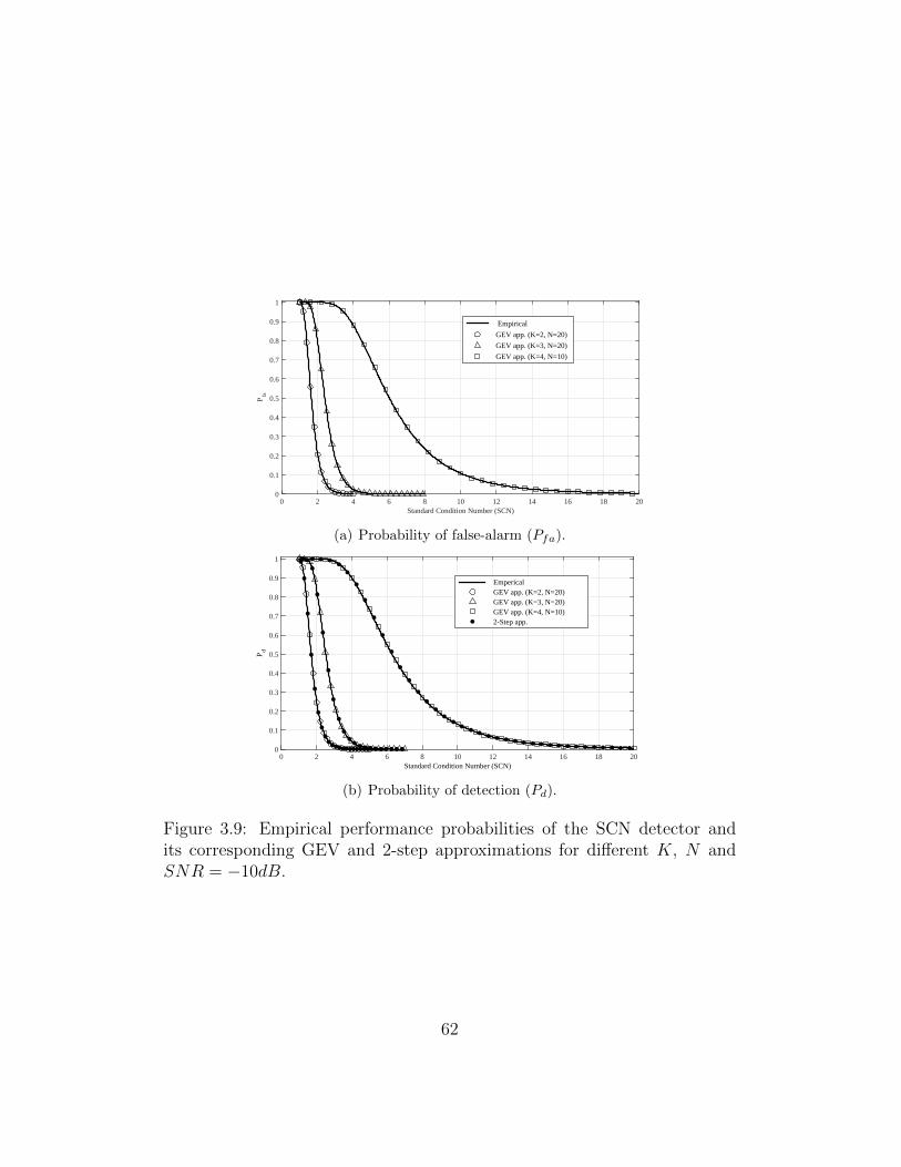
Standard Condition Number (SCN)0 2 4 6 8 10 12 14 16 18 20
Pfa
0
0.1
0.2
0.3
0.4
0.5
0.6
0.7
0.8
0.9
1
Empirical
GEV app. (K=2, N=20)
GEV app. (K=3, N=20)
GEV app. (K=4, N=10)
(a) Probability of false-alarm (Pfa).
Standard Condition Number (SCN)0 2 4 6 8 10 12 14 16 18 20
Pd
0
0.1
0.2
0.3
0.4
0.5
0.6
0.7
0.8
0.9
1
Emperical GEV app. (K=2, N=20) GEV app. (K=3, N=20) GEV app. (K=4, N=10) 2-Step app.
(b) Probability of detection (Pd).
Figure 3.9: Empirical performance probabilities of the SCN detector andits corresponding GEV and 2-step approximations for different K, N andSNR = −10dB.
62
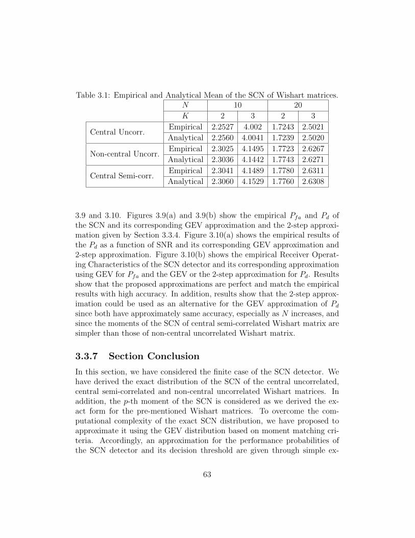
Table 3.1: Empirical and Analytical Mean of the SCN of Wishart matrices.N 10 20
K 2 3 2 3
Central Uncorr.Empirical 2.2527 4.002 1.7243 2.5021
Analytical 2.2560 4.0041 1.7239 2.5020
Non-central Uncorr.Empirical 2.3025 4.1495 1.7723 2.6267
Analytical 2.3036 4.1442 1.7743 2.6271
Central Semi-corr.Empirical 2.3041 4.1489 1.7780 2.6311
Analytical 2.3060 4.1529 1.7760 2.6308
3.9 and 3.10. Figures 3.9(a) and 3.9(b) show the empirical Pfa and Pd ofthe SCN and its corresponding GEV approximation and the 2-step approxi-mation given by Section 3.3.4. Figure 3.10(a) shows the empirical results ofthe Pd as a function of SNR and its corresponding GEV approximation and2-step approximation. Figure 3.10(b) shows the empirical Receiver Operat-ing Characteristics of the SCN detector and its corresponding approximationusing GEV for Pfa and the GEV or the 2-step approximation for Pd. Resultsshow that the proposed approximations are perfect and match the empiricalresults with high accuracy. In addition, results show that the 2-step approx-imation could be used as an alternative for the GEV approximation of Pdsince both have approximately same accuracy, especially as N increases, andsince the moments of the SCN of central semi-correlated Wishart matrix aresimpler than those of non-central uncorrelated Wishart matrix.
3.3.7 Section Conclusion
In this section, we have considered the finite case of the SCN detector. Wehave derived the exact distribution of the SCN of the central uncorrelated,central semi-correlated and non-central uncorrelated Wishart matrices. Inaddition, the p-th moment of the SCN is considered as we derived the ex-act form for the pre-mentioned Wishart matrices. To overcome the com-putational complexity of the exact SCN distribution, we have proposed toapproximate it using the GEV distribution based on moment matching cri-teria. Accordingly, an approximation for the performance probabilities ofthe SCN detector and its decision threshold are given through simple ex-
63
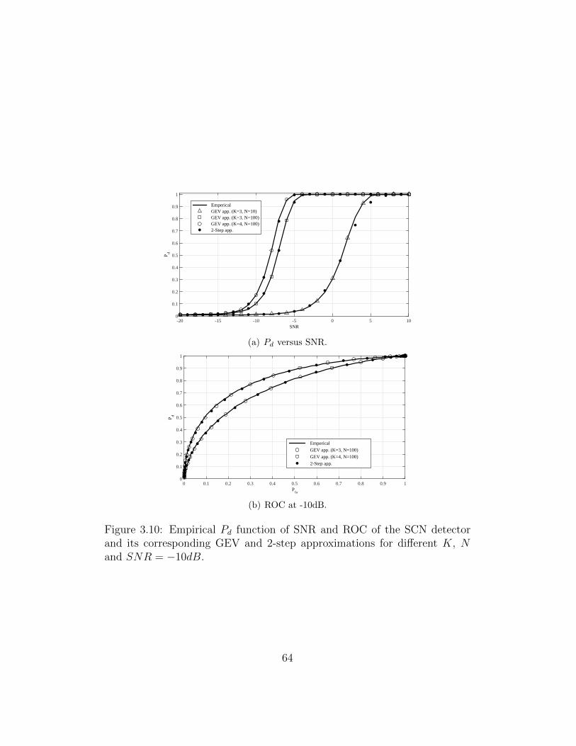
SNR-20 -15 -10 -5 0 5 10
Pd
0
0.1
0.2
0.3
0.4
0.5
0.6
0.7
0.8
0.9
1
Emperical GEV app. (K=3, N=10) GEV app. (K=3, N=100) GEV app. (K=4, N=100) 2-Step app.
(a) Pd versus SNR.
Pfa
0 0.1 0.2 0.3 0.4 0.5 0.6 0.7 0.8 0.9 1
Pd
0
0.1
0.2
0.3
0.4
0.5
0.6
0.7
0.8
0.9
1
Emperical
GEV app. (K=3, N=100)
GEV app. (K=4, N=100)
2-Step app.
(b) ROC at -10dB.
Figure 3.10: Empirical Pd function of SNR and ROC of the SCN detectorand its corresponding GEV and 2-step approximations for different K, Nand SNR = −10dB.
64
pressions. Moreover, and using the non-central/central approximation wehave proposed a 2-step approximation for the detection probability of theSCN detector which provides analogous accuracy with simpler moment com-plexity. The analytical results are validated through extensive Monte-Carlosimulations with different system parameters. Results have shown that theproposed GEV approximation perfectly fits the empirical results.
3.4 Asymptotic Case
In literature, the SCN metric was studied asymptotically in [36] and thethreshold was presented according to Marchenko-Pastur (MP) law [185]. Ifthe size of the receiver’s matrix is K×N , then MP law proves that the largestand the smallest eigenvalues of the receiver’s covariance matrix converge toconstants as (K,N) → ∞ with c = K/N [46]. These constants are simplydetermined by the constant c and the noise and signal powers. In [38], theauthors improved the accuracy of the asymptotic statistical distribution ofthe SCN by using the Tracy-Widom (TW) distribution to model the largesteigenvalue [186] while maintaining the MP representation of the smallest one.TW distribution is a limiting distribution of the largest eigenvalue of a cen-tral Wishart matrix as (K,N)→∞ [187]. This approximation of the SCN,by TW distribution for the numerator and MP law for the denominator,results in an approximated relation between the decision threshold and thePfa. This work was further extended in [37, 188] by using Curtiss formulafor the distribution of the ratio of random variables [189] where both thelargest and the smallest eigenvalues converge to Tracy-Widom distributionswhen (K,N) → ∞ as shown in [186, 190]. Moreover, by the exploitationof the normal and TW distributions and using the Curtiss formula, the au-thors in [191] provided an analytical expression for the probability of Pmd forsufficiently large values of K and N . However, all these expressions includeTW distribution and Curtiss formula that are hard to evaluate numericallyonline.
The importance of the GEV approximation provided by the previoussection is indeed due to its accuracy and simplicity. However, the exactexpressions of the moments are still complicated and need to be computedoffline. In this section, we will show that a simple form approximation forthese moments could be derived under certain conditions. We will first con-sider some statistical properties of the extreme eigenvalues of W and analyze
65

these properties under both detection hypothesis in Sec. 3.4.1.Since SCN is not affected by the noise power, let σ2
η = 1 and we definethe Asymptotic Condition (AC) and the Critical Condition (CC) as follows:
AC : (K,N)→∞ with K/N → c ∈ (0, 1), (3.49)
CC : ρ > ρc =1√KN
. (3.50)
3.4.1 Assymptotic Moments of Extreme Eigenvalues
This section considers the statistical analysis of the extreme eigenvalues, λ1
and λK , of the sample covariance matrix, W , by considering both hypothesesH0 and H1.
H0 hypothesis
Let λH01 be the largest eigenvalue of W under H0 and denote the centered
and scaled version of λH01 of the central uncorrelated complex Wishart matrix
W ∼ CWK(N, IK) by:
λ′1 =λH0
1 − a1(K,N)
b1(K,N)(3.51)
with a1(K,N) and b1(K,N), the centering and scaling coefficients respec-tively, are defined by:
a1(K,N) = (√K +
√N)2 (3.52)
b1(K,N) = (√K +
√N)(K−1/2 +N−1/2)
13 (3.53)
then, as AC is satisfied, λ′1 follows a TW distribution of order 2 (TW2) [192].Now let λH0
K be the smallest eigenvalue ofW underH0 and denote the cen-tered and scaled version of λH0
K of the central uncorrelated complex Wishartmatrix W ∼ CWK(N, IK) by:
λ′K =λH0K − a2(K,N)
b2(K,N)(3.54)
with a2(K,N) and b2(K,N), the centering and scaling coefficients respec-tively, are defined by:
a2(K,N) = (√K −
√N)2 (3.55)
b2(K,N) = (√K −
√N)(K−1/2 −N−1/2)
13 (3.56)
66
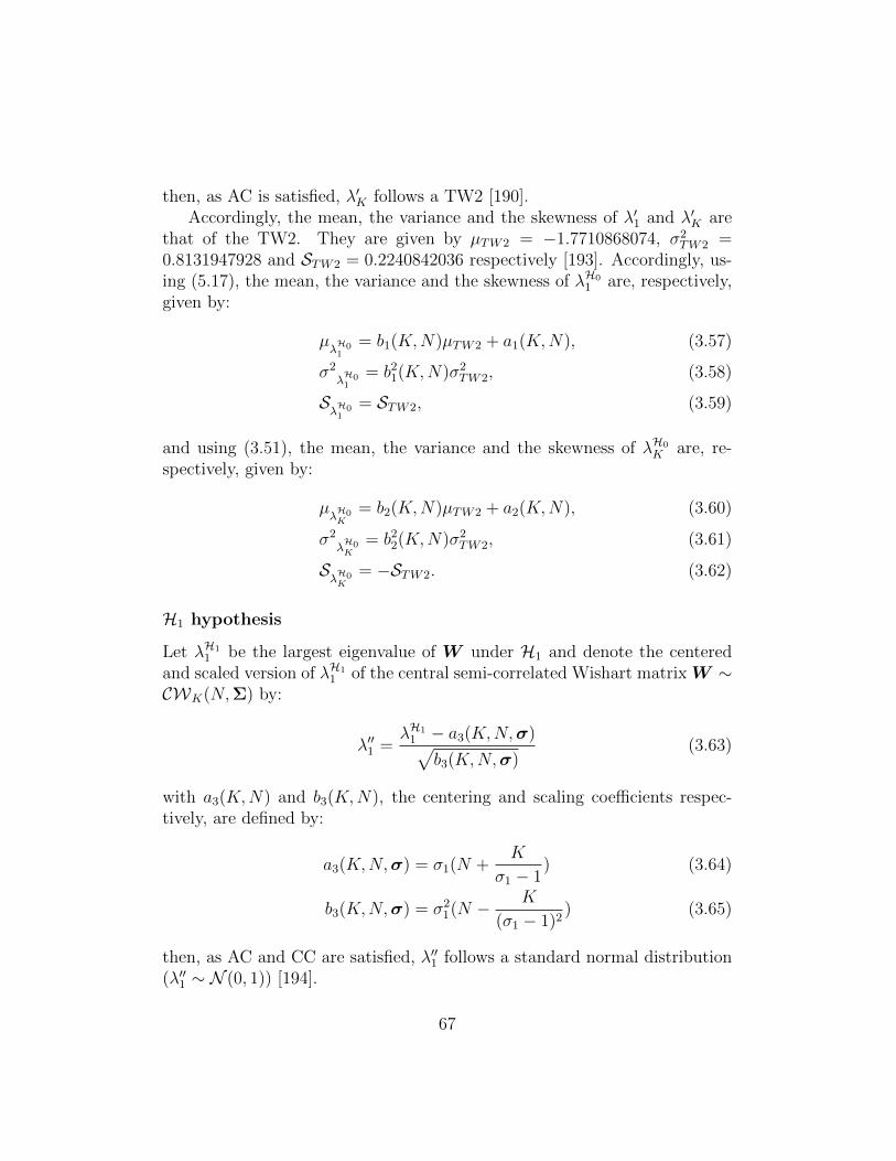
then, as AC is satisfied, λ′K follows a TW2 [190].Accordingly, the mean, the variance and the skewness of λ′1 and λ′K are
that of the TW2. They are given by µTW2 = −1.7710868074, σ2TW2 =
0.8131947928 and STW2 = 0.2240842036 respectively [193]. Accordingly, us-ing (5.17), the mean, the variance and the skewness of λH0
1 are, respectively,given by:
µλH01
= b1(K,N)µTW2 + a1(K,N), (3.57)
σ2λH01
= b21(K,N)σ2
TW2, (3.58)
SλH01
= STW2, (3.59)
and using (3.51), the mean, the variance and the skewness of λH0K are, re-
spectively, given by:
µλH0K
= b2(K,N)µTW2 + a2(K,N), (3.60)
σ2λH0K
= b22(K,N)σ2
TW2, (3.61)
SλH0K
= −STW2. (3.62)
H1 hypothesis
Let λH11 be the largest eigenvalue of W under H1 and denote the centered
and scaled version of λH11 of the central semi-correlated Wishart matrix W ∼
CWK(N,Σ) by:
λ′′1 =λH1
1 − a3(K,N,σ)√b3(K,N,σ)
(3.63)
with a3(K,N) and b3(K,N), the centering and scaling coefficients respec-tively, are defined by:
a3(K,N,σ) = σ1(N +K
σ1 − 1) (3.64)
b3(K,N,σ) = σ21(N − K
(σ1 − 1)2) (3.65)
then, as AC and CC are satisfied, λ′′1 follows a standard normal distribution(λ′′1 ∼ N (0, 1)) [194].
67
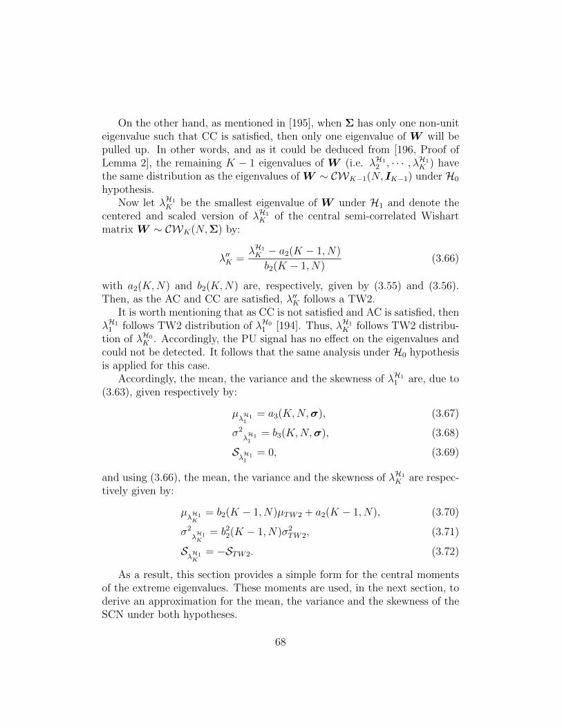
On the other hand, as mentioned in [195], when Σ has only one non-uniteigenvalue such that CC is satisfied, then only one eigenvalue of W will bepulled up. In other words, and as it could be deduced from [196, Proof ofLemma 2], the remaining K − 1 eigenvalues of W (i.e. λH1
2 , · · · , λH1K ) have
the same distribution as the eigenvalues of W ∼ CWK−1(N, IK−1) under H0
hypothesis.Now let λH1
K be the smallest eigenvalue of W under H1 and denote thecentered and scaled version of λH1
K of the central semi-correlated Wishartmatrix W ∼ CWK(N,Σ) by:
λ′′K =λH1K − a2(K − 1, N)
b2(K − 1, N)(3.66)
with a2(K,N) and b2(K,N) are, respectively, given by (3.55) and (3.56).Then, as the AC and CC are satisfied, λ′′K follows a TW2.
It is worth mentioning that as CC is not satisfied and AC is satisfied, thenλH1
1 follows TW2 distribution of λH01 [194]. Thus, λH1
K follows TW2 distribu-tion of λH0
K . Accordingly, the PU signal has no effect on the eigenvalues andcould not be detected. It follows that the same analysis under H0 hypothesisis applied for this case.
Accordingly, the mean, the variance and the skewness of λH11 are, due to
(3.63), given respectively by:
µλH11
= a3(K,N,σ), (3.67)
σ2λH11
= b3(K,N,σ), (3.68)
SλH11
= 0, (3.69)
and using (3.66), the mean, the variance and the skewness of λH1K are respec-
tively given by:
µλH1K
= b2(K − 1, N)µTW2 + a2(K − 1, N), (3.70)
σ2λH1K
= b22(K − 1, N)σ2
TW2, (3.71)
SλH1K
= −STW2. (3.72)
As a result, this section provides a simple form for the central momentsof the extreme eigenvalues. These moments are used, in the next section, toderive an approximation for the mean, the variance and the skewness of theSCN under both hypotheses.
68
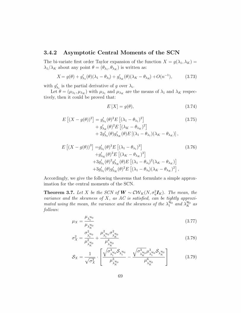
3.4.2 Asymptotic Central Moments of the SCN
The bi-variate first order Taylor expansion of the function X = g(λ1, λK) =λ1/λK about any point θ = (θλ1 , θλK ) is written as:
X= g(θ) + g′λ1(θ)(λ1 − θλ1) + g′λK (θ)(λK − θλK) +O(n−1), (3.73)
with g′λi is the partial derivative of g over λi.Let θ = (µλ1 , µλK ) with µλ1 and µλK are the means of λ1 and λK respec-
tively, then it could be proved that:
E [X] = g(θ), (3.74)
E[(X − g(θ))2
]= g′λ1
(θ)2E[(λ1 − θλ1)2
](3.75)
+ g′λK (θ)2E[(λK − θλK )2
]+ 2g′λ1
(θ)g′λK (θ)E [(λ1 − θλ1)(λK − θλK )] ,
E[(X − g(θ))3] =g′λ1
(θ)3E[(λ1 − θλ1)3
](3.76)
+g′λK (θ)3E[(λK − θλK )3
]+3g′λ1
(θ)2g′λK (θ)E[(λ1 − θλ1)
2(λK − θλK )]
+3g′λ1(θ)g′λK (θ)2E
[(λ1 − θλ1)(λK − θλK )2
],
Accordingly, we give the following theorems that formulate a simple approx-imation for the central moments of the SCN.
Theorem 3.7. Let X be the SCN of W ∼ CWK(N, σ2ηIK). The mean, the
variance and the skewness of X, as AC is satisfied, can be tightly approxi-mated using the mean, the variance and the skewness of the λH0
1 and λH0K as
follows:
µX =µλH01
µλH0K
(3.77)
σ2X =
σ2
λH01
µ2
λH0K
+µ2
λH01
σ2
λH0K
µ4
λH0K
(3.78)
SX =1√σ3X
·
√σ3
λH01
SλH01
µ3
λH0K
−
√σ3
λH0K
µ3
λH01
SλH0K
µ6
λH0K
(3.79)
69
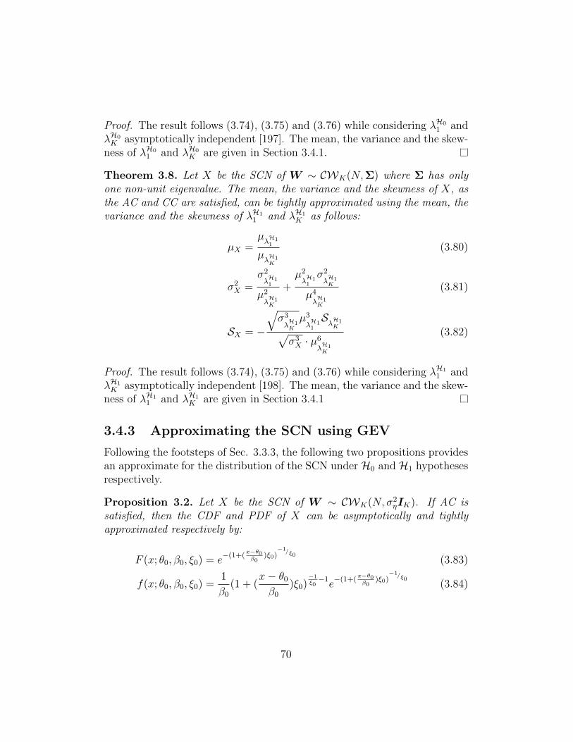
Proof. The result follows (3.74), (3.75) and (3.76) while considering λH01 and
λH0K asymptotically independent [197]. The mean, the variance and the skew-
ness of λH01 and λH0
K are given in Section 3.4.1.
Theorem 3.8. Let X be the SCN of W ∼ CWK(N,Σ) where Σ has onlyone non-unit eigenvalue. The mean, the variance and the skewness of X, asthe AC and CC are satisfied, can be tightly approximated using the mean, thevariance and the skewness of λH1
1 and λH1K as follows:
µX =µλH11
µλH1K
(3.80)
σ2X =
σ2
λH11
µ2
λH1K
+µ2
λH11
σ2
λH1K
µ4
λH1K
(3.81)
SX = −
√σ3
λH1K
µ3
λH11
SλH1K√
σ3X · µ6
λH1K
(3.82)
Proof. The result follows (3.74), (3.75) and (3.76) while considering λH11 and
λH1K asymptotically independent [198]. The mean, the variance and the skew-
ness of λH11 and λH1
K are given in Section 3.4.1
3.4.3 Approximating the SCN using GEV
Following the footsteps of Sec. 3.3.3, the following two propositions providesan approximate for the distribution of the SCN under H0 and H1 hypothesesrespectively.
Proposition 3.2. Let X be the SCN of W ∼ CWK(N, σ2ηIK). If AC is
satisfied, then the CDF and PDF of X can be asymptotically and tightlyapproximated respectively by:
F (x; θ0, β0, ξ0) = e−(1+(
x−θ0β0
)ξ0)−1/ξ0
(3.83)
f(x; θ0, β0, ξ0) =1
β0
(1 + (x− θ0
β0
)ξ0)−1ξ0−1e−(1+(
x−θ0β0
)ξ0)−1/ξ0
(3.84)
70
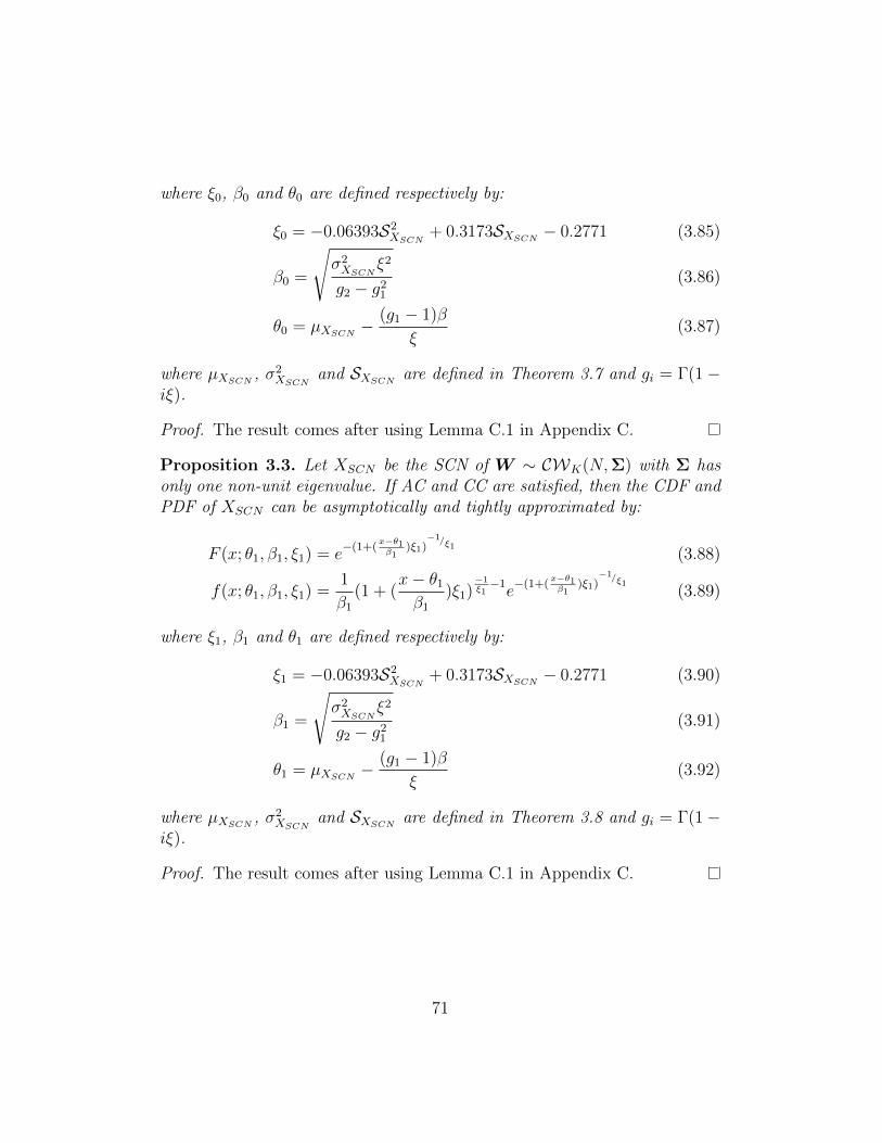
where ξ0, β0 and θ0 are defined respectively by:
ξ0 = −0.06393S2XSCN
+ 0.3173SXSCN − 0.2771 (3.85)
β0 =
√σ2XSCN
ξ2
g2 − g21
(3.86)
θ0 = µXSCN −(g1 − 1)β
ξ(3.87)
where µXSCN , σ2XSCN
and SXSCN are defined in Theorem 3.7 and gi = Γ(1−iξ).
Proof. The result comes after using Lemma C.1 in Appendix C.
Proposition 3.3. Let XSCN be the SCN of W ∼ CWK(N,Σ) with Σ hasonly one non-unit eigenvalue. If AC and CC are satisfied, then the CDF andPDF of XSCN can be asymptotically and tightly approximated by:
F (x; θ1, β1, ξ1) = e−(1+(
x−θ1β1
)ξ1)−1/ξ1
(3.88)
f(x; θ1, β1, ξ1) =1
β1
(1 + (x− θ1
β1
)ξ1)−1ξ1−1e−(1+(
x−θ1β1
)ξ1)−1/ξ1
(3.89)
where ξ1, β1 and θ1 are defined respectively by:
ξ1 = −0.06393S2XSCN
+ 0.3173SXSCN − 0.2771 (3.90)
β1 =
√σ2XSCN
ξ2
g2 − g21
(3.91)
θ1 = µXSCN −(g1 − 1)β
ξ(3.92)
where µXSCN , σ2XSCN
and SXSCN are defined in Theorem 3.8 and gi = Γ(1−iξ).
Proof. The result comes after using Lemma C.1 in Appendix C.
71
3.4.4 Performance Probabilities and Decission Thresh-old
Based on Propositions 3.2 and 3.3, and using (2.6), (2.7) and (2.8), the Pfaand Pd are respectively expressed as:
Pfa = 1− e−(1+(λSCN−θ0
β0)ξ0)−1/ξ0
, (3.93)
Pmd = 1− Pd = e−(1+(
λSCN−θ1β1
)ξ1)−1/ξ1
. (3.94)
The threshold could be computed using (3.93) and (3.94) according to arequired error constraint. For example, for a target false alarm probability,the threshold is given by:
λSCN = θ0 +β0
ξ0
(− 1 +
[− ln(1− Pfa)
]−ξ0). (3.95)
3.4.5 Numerical Results and Discussion
In this section, we verify the analytical derivation results through Monte-Carlo simulations. We validate the theoretical analysis presented in sections3.4.1, 3.4.2, 3.4.3 and 3.4.4.
Table 3.2 shows the accuracy of the analytical approximation of the mean,the variance and the skewness of the SCN provided by Theorems 3.7 and 3.8.It can be easily seen that these Theorems provide a good approximation forthe statistics of the SCN, however, it could be noticed that the skewness isnot perfectly approximated. In fact, the skewness is affected by the slow con-vergence of the skewness of λK that must converge to −STW2 (i.e. −0.2241)as AC is satisfied. For example, for K = 50, the empirical skewness increasesfrom SλK = −0.1504 to SλK = −0.1819 as the number of samples increasesfrom N = 500 to N = 1000. Comparing these results with SCN results inTable 3.2, one can notice that the empirical and approximated SCN skew-ness become closer as λK skewness converges to that of TW2. Accordingly,Theorems 3.7 and 3.8 are good approximations for the mean, the varianceand the skewness of the SCN under both hypotheses. It is worth notingthat one could approximate the SCN moments using second order bi-variateTaylor series to get a slightly higher accuracy, however, this will cost highercomplexity and it is not necessary as shown in Table 3.2 and the rest of thissection.
72
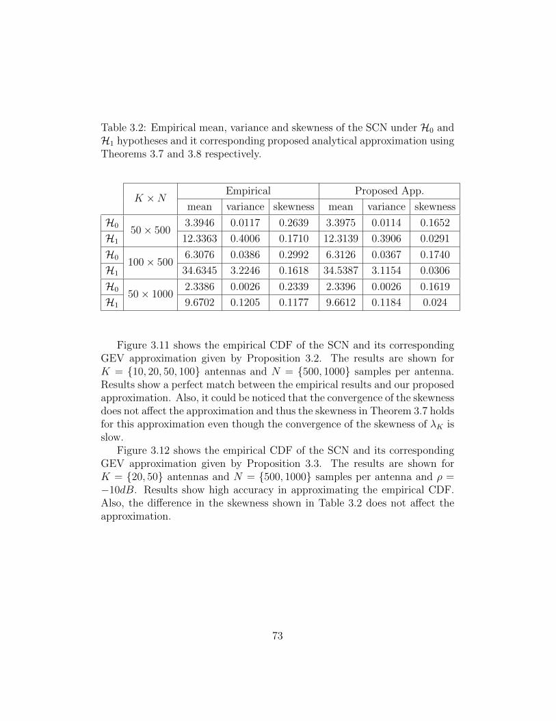
Table 3.2: Empirical mean, variance and skewness of the SCN under H0 andH1 hypotheses and it corresponding proposed analytical approximation usingTheorems 3.7 and 3.8 respectively.
K ×N Empirical Proposed App.
mean variance skewness mean variance skewness
H050× 500
3.3946 0.0117 0.2639 3.3975 0.0114 0.1652
H1 12.3363 0.4006 0.1710 12.3139 0.3906 0.0291
H0100× 500
6.3076 0.0386 0.2992 6.3126 0.0367 0.1740
H1 34.6345 3.2246 0.1618 34.5387 3.1154 0.0306
H050× 1000
2.3386 0.0026 0.2339 2.3396 0.0026 0.1619
H1 9.6702 0.1205 0.1177 9.6612 0.1184 0.024
Figure 3.11 shows the empirical CDF of the SCN and its correspondingGEV approximation given by Proposition 3.2. The results are shown forK = 10, 20, 50, 100 antennas and N = 500, 1000 samples per antenna.Results show a perfect match between the empirical results and our proposedapproximation. Also, it could be noticed that the convergence of the skewnessdoes not affect the approximation and thus the skewness in Theorem 3.7 holdsfor this approximation even though the convergence of the skewness of λK isslow.
Figure 3.12 shows the empirical CDF of the SCN and its correspondingGEV approximation given by Proposition 3.3. The results are shown forK = 20, 50 antennas and N = 500, 1000 samples per antenna and ρ =−10dB. Results show high accuracy in approximating the empirical CDF.Also, the difference in the skewness shown in Table 3.2 does not affect theapproximation.
73
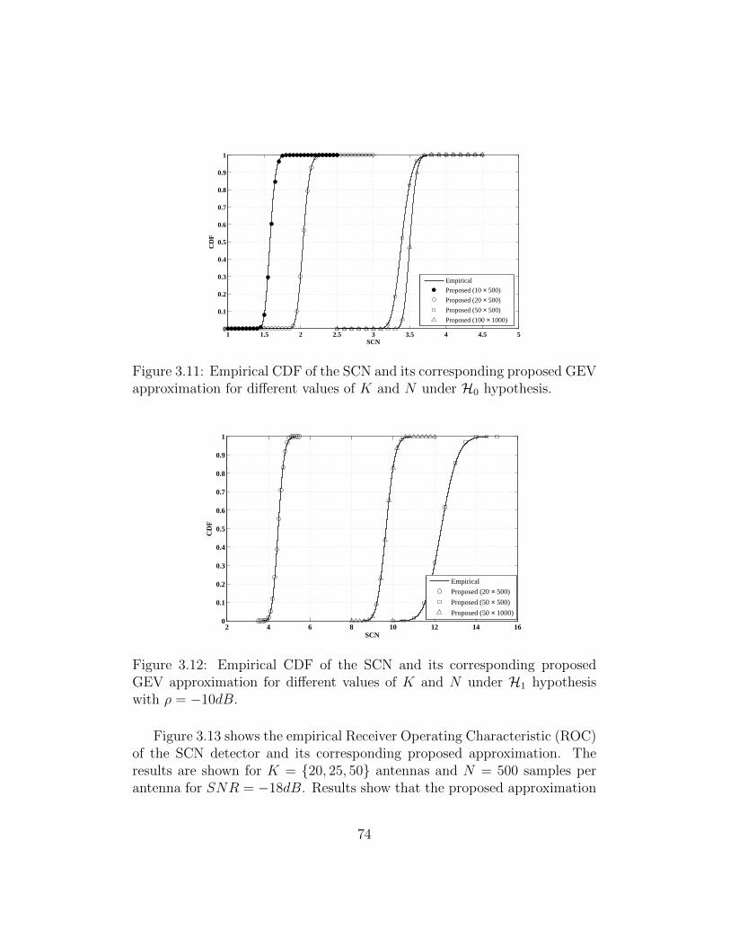
1 1.5 2 2.5 3 3.5 4 4.5 50
0.1
0.2
0.3
0.4
0.5
0.6
0.7
0.8
0.9
1
SCN
CD
F
Empirical
Proposed (10 × 500)
Proposed (20 × 500)
Proposed (50 × 500)
Proposed (100 × 1000)
Figure 3.11: Empirical CDF of the SCN and its corresponding proposed GEVapproximation for different values of K and N under H0 hypothesis.
2 4 6 8 10 12 14 160
0.1
0.2
0.3
0.4
0.5
0.6
0.7
0.8
0.9
1
SCN
CD
F
Empirical
Proposed (20 × 500)
Proposed (50 × 500)
Proposed (50 × 1000)
Figure 3.12: Empirical CDF of the SCN and its corresponding proposedGEV approximation for different values of K and N under H1 hypothesiswith ρ = −10dB.
Figure 3.13 shows the empirical Receiver Operating Characteristic (ROC)of the SCN detector and its corresponding proposed approximation. Theresults are shown for K = 20, 25, 50 antennas and N = 500 samples perantenna for SNR = −18dB. Results show that the proposed approximation
74
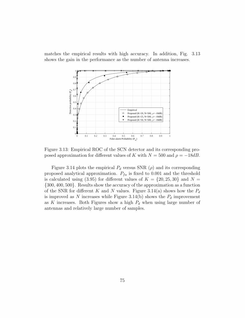
matches the empirical results with high accuracy. In addition, Fig. 3.13shows the gain in the performance as the number of antenna increases.
False-alarm Probability (Pfa
)0 0.1 0.2 0.3 0.4 0.5 0.6 0.7 0.8 0.9 1
Det
ectio
n pr
obab
ility
(P d)
0
0.1
0.2
0.3
0.4
0.5
0.6
0.7
0.8
0.9
1
Empirical
Proposed (K=20, N=500, ρ= -18dB)
Proposed (K=25, N=500, ρ= -18dB)
Proposed (K=50, N=500, ρ= -18dB)
Figure 3.13: Empirical ROC of the SCN detector and its corresponding pro-posed approximation for different values of K with N = 500 and ρ = −18dB.
Figure 3.14 plots the empirical Pd versus SNR (ρ) and its correspondingproposed analytical approximation. Pfa is fixed to 0.001 and the thresholdis calculated using (3.95) for different values of K = 20, 25, 30 and N =300, 400, 500. Results show the accuracy of the approximation as a functionof the SNR for different K and N values. Figure 3.14(a) shows how the Pdis improved as N increases while Figure 3.14(b) shows the Pd improvementas K increases. Both Figures show a high Pd when using large number ofantennas and relatively large number of samples.
75
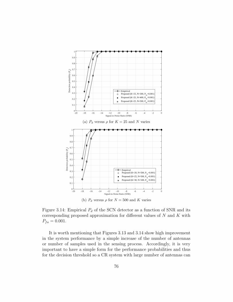
Signal-to-Noise Ratio (SNR)-20 -18 -16 -14 -12 -10 -8 -6 -4 -2 0
Det
ectio
n pr
obab
ility
(P d)
0
0.1
0.2
0.3
0.4
0.5
0.6
0.7
0.8
0.9
1
Empirical Proposed (K=25, N=300, P
fa=0.001)
Proposed (K=25, N=400, Pfa
=0.001)
Proposed (K=25, N=500, Pfa
=0.001)
(a) Pd versus ρ for K = 25 and N varies
Signal-to-Noise Ratio (SNR)-20 -18 -16 -14 -12 -10 -8 -6 -4 -2 0
Det
ectio
n pr
obab
ility
(P d)
0
0.1
0.2
0.3
0.4
0.5
0.6
0.7
0.8
0.9
1
EmpiricalProposed (K=20, N=500, P
fa=0.001)
Proposed (K=25, N=500, Pfa
=0.001)
Proposed (K=30, N=500, Pfa
=0.001)
(b) Pd versus ρ for N = 500 and K varies
Figure 3.14: Empirical Pd of the SCN detector as a function of SNR and itscorresponding proposed approximation for different values of N and K withPfa = 0.001.
It is worth mentioning that Figures 3.13 and 3.14 show high improvementin the system performance by a simple increase of the number of antennasor number of samples used in the sensing process. Accordingly, it is veryimportant to have a simple form for the performance probabilities and thusfor the decision threshold so a CR system with large number of antennas can
76
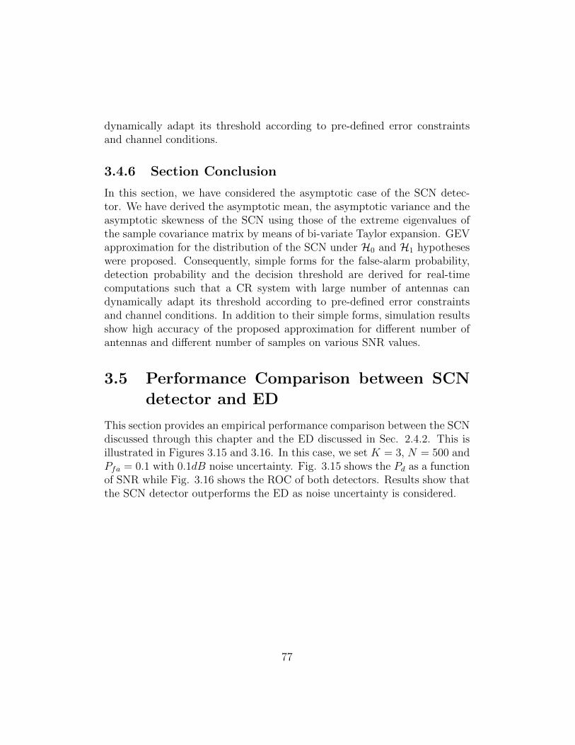
dynamically adapt its threshold according to pre-defined error constraintsand channel conditions.
3.4.6 Section Conclusion
In this section, we have considered the asymptotic case of the SCN detec-tor. We have derived the asymptotic mean, the asymptotic variance and theasymptotic skewness of the SCN using those of the extreme eigenvalues ofthe sample covariance matrix by means of bi-variate Taylor expansion. GEVapproximation for the distribution of the SCN under H0 and H1 hypotheseswere proposed. Consequently, simple forms for the false-alarm probability,detection probability and the decision threshold are derived for real-timecomputations such that a CR system with large number of antennas candynamically adapt its threshold according to pre-defined error constraintsand channel conditions. In addition to their simple forms, simulation resultsshow high accuracy of the proposed approximation for different number ofantennas and different number of samples on various SNR values.
3.5 Performance Comparison between SCN
detector and ED
This section provides an empirical performance comparison between the SCNdiscussed through this chapter and the ED discussed in Sec. 2.4.2. This isillustrated in Figures 3.15 and 3.16. In this case, we set K = 3, N = 500 andPfa = 0.1 with 0.1dB noise uncertainty. Fig. 3.15 shows the Pd as a functionof SNR while Fig. 3.16 shows the ROC of both detectors. Results show thatthe SCN detector outperforms the ED as noise uncertainty is considered.
77
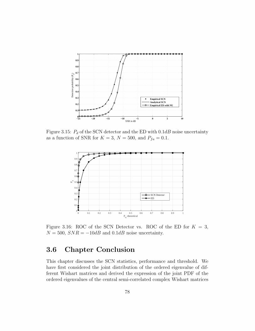
−25 −20 −15 −10 −5 0 5 100
0.1
0.2
0.3
0.4
0.5
0.6
0.7
0.8
0.9
1
SNR in dB
Det
ectio
n pr
obab
ility
(P d)
Empirical SCNAnalytical SCNEmpirical ED with NU
Figure 3.15: Pd of the SCN detector and the ED with 0.1dB noise uncertaintyas a function of SNR for K = 3, N = 500, and Pfa = 0.1.
Pfa
-theoretical0 0.1 0.2 0.3 0.4 0.5 0.6 0.7 0.8 0.9 1
Pd
0
0.1
0.2
0.3
0.4
0.5
0.6
0.7
0.8
0.9
1
SCN DetectorED
Figure 3.16: ROC of the SCN Detector vs. ROC of the ED for K = 3,N = 500, SNR = −10dB and 0.1dB noise uncertainty.
3.6 Chapter Conclusion
This chapter discusses the SCN statistics, performance and threshold. Wehave first considered the joint distribution of the ordered eigenvalue of dif-ferent Wishart matrices and derived the expression of the joint PDF of theordered eigenvalues of the central semi-correlated complex Wishart matrices
78
when the correlation matrix exhibit equal eigenvalues. The non-central/centralapproximation is empirically studied and results show that it has perfect ac-curacy in low SNR regions and could be considered as a good fit for Pd forsufficiently large values of N when the SNR is high. Moreover, in the fi-nite case, We have derived the exact distribution of the SCN of the centraluncorrelated, central semi-correlated and non-central uncorrelated Wishartmatrices. In addition, the p-th moment of the SCN is considered as wederived the exact form for the pre-mentioned Wishart matrices. To over-come the computational complexity of the exact SCN distribution, we haveproposed to approximate it using the GEV distribution based on momentmatching criteria. Accordingly, an approximation for the performance prob-abilities of the SCN detector and its decision threshold are given throughsimple expressions. Moreover, and using the non-central/central approxima-tion we have proposed a 2-step approximation for the detection probability ofthe SCN detector which provides analogous accuracy with simpler momentcomplexity. Finally, in the asymptotic case, We have derived the asymptoticmean, the asymptotic variance and the asymptotic skewness of the SCN usingthose of the extreme eigenvalues of the sample covariance matrix by meansof bi-variate Taylor expansion. GEV approximation for the distribution ofthe SCN under H0 and H1 hypotheses were proposed. Consequently, simpleforms for the false-alarm probability, detection probability and the decisionthreshold are derived for real-time computations such that a CR system withlarge number of antennas can dynamically adapt its threshold according topre-defined error constraints and channel conditions. The analytical resultsare validated through extensive Monte-Carlo simulations with different sys-tem parameters. Results show high accuracy of the proposed approximationfor different number of antennas and different number of samples on variousSNR values.
79
Chapter 4
Scaled largest Eigenvalue
Detector: A Simple
Formulation Approach
This chapter considers the performance probabilities and the decision thresh-old of the SLE detector. Consequently, it discusses the statistical distributionof the SLE decision metric of the SLE detector. First, the distribution of thelargest eigenvalue and the trace of the Wishart matrix are considered andour contributions are presented in Sec. 4.2. Subsequently, the distribution ofthe SLE decision metric is derived in Sec. 4.3. The performance probabilitiesand the decision threshold are also considered. The correlation between thelargest eigenvalue and the trace is then considered in Sec. 4.4. Finally, allour contributions are validated in Sec. 4.5 using numerical simulations.
4.1 Scaled Largest Eigenvalue
In the literature, several eigenvalue ratios have been considered as discussedin Sec. 2.5. The SCN ratio has been extensively studied and has manyapplications mainly in the context of MIMO systems and SS as mentionedin Ch. 3. On the other hand, Scaled Largest Eigenvalue detector (SLE) isanother eigenvalue ratio measure that recently received an important atten-tion. SLE detector is an efficient technique that is proved to be the optimaldetector under the Generalized Likelihood Ratio (GLR) criterion and noise
80
uncertainty environments [40, 41]. Indeed, it is a practical scenario since inpractical systems the noise power may not be perfectly known. Moreover,since Spectrum Sensing (SS) is the task of obtaining awareness about thespectrum usage, as presented in Chapter 2, then it mainly concerns two sce-narios of detection: (i) detecting the absence of the Primary User (PU) ina licensed spectrum in order for the Secondary User (SU) to use it and (ii)detecting the presence of the PU so the SU avoid the channel, stop transmis-sion or switch to another channel to avoid any interference to the PrimaryReceiver (PR). Hence, SS plays a major role in the performance of the CRas well as in the performance of the PU network. In this context, an extremeimportance for a CR network is to have an optimal SS technique with highaccuracy in uncertain environments.
Recall the SLE decision metric from (2.26):
XSLE =λ1
1K
∑Ki=1 λi
(4.1)
Before it was introduced to CR [199], the SLE previously appeared insignal processing [200] and statistics literature [201, 202]. SLE detector is atotally-blind detector, which is not effected by noise power uncertainty andwhich stands out as the optimal single-PU detector as mentioned. For agiven decision threshold, λSLE, the SLE detector algorithm could be done byusing one of Algorithms 4.1 and 4.2 given below.
Algorithm 4.1: SLE Detector using EVD
Input: Y , λSLEOutput: DSLE
1 compute W = Y Y † ;2 get λ1≤i≤K of W in descending order;
3 evaluate XSLE = λ11K
∑λi
;
4 decide DSLE = XSLE
H1
≷H0
λSLE ;
The results on the statistics of the SLE, in the literature, are relativelylimited. They are based on tools from Random Matrix Theory (RMT)[40, 203, 204] and Mellin transform [204–206]. SLE was considered, asymp-totically, to follow the LE distribution (i.e. TW distribution) [40]. However,
81
Algorithm 4.2: SLE Detector using Power method
Input: Y , λSLEOutput: DSLE
1 compute W = Y Y † ;2 compute tr(W ) ;3 get λ1 of W using Power method;
4 evaluate XSLE = λ11Ktr(W )
;
5 decide DSLE = XSLE
H1
≷H0
λSLE ;
a non-negligible error still exists and a new form was derived based on theTW distribution and its second derivative [203]. Using Mellin transform, Thedistribution of the SLE was derived by the exploitation of the distributionof LE and the distribution of the trace [204–206]. However, all the findingson SLE are too complex to be considered in real-environments and hence arenot easily scalable. This is due to either a complexity in the original distri-butions used to model the SLE (e.g. the TW distribution) or in the methodsused to derive the thresholds. Hence, there is a necessity to propose novelyet simple forms in both SS cases (presence and absence of PU activity).
In this chapter, we tackle this problem by considering simple solutiondeduced from the properties of the LE and trace of the Wishart matrices. Inthis regard, we start by considering the LE of the Wishart matrices underH0 and H1 hypothesis. After that the distribution of the trace is consideredto end up with a new form distribution of the SLE decision metric.
4.2 LE and Trace Distributions
This section considers the distributions of the LE and of the trace under H0
and H1 hypothesis. We prove that the LE and the trace follow Gaussiandistributions for which the means and variances are formulated. Since theSLE does not depend on the noise power, we suppose, in this section, thatσ2η = 1. Based on the results of this section, we derive the distribution of the
SLE in the next section.
82
4.2.1 Largest Eigenvalue Distribution
It has been shown that, for a fixed K and as N →∞, λH01 follows a normal
distribution under H0 hypothesis [150, 207]. The mean and the variance ofλH0
1 could be approximated using TW2 and they are, respectively, given by :
µλH01
= b1(K,N)µTW2 + a1(K,N), (4.2)
σ2λH01
= b21(K,N)σ2
TW2, (4.3)
where µTW2 = −1.7710868074 and σ2TW2 = 0.8131947928 are, respectively,
the mean and variance of TW2 distribution; a1(K,N) and b1(K,N) are re-spectively given by (3.52) and (3.53) as follows:
a1(K,N) = (√K +
√N)2, (4.4)
b1(K,N) = (√K +
√N)(K−1/2 +N−1/2)
13 . (4.5)
This approximation is very efficient and it achieves high accuracy for Kas small as 2 [150].
On the other hand, Recall that the Asymptotic Condition (AC) and theCritical Condition (CC) are defined as follows:
AC : (K,N)→∞ with K/N → c ∈ (0, 1), (4.6)
CC : ρ > ρc =1√KN
, (4.7)
then as mentioned in Sec. 3.4.1, as AC and CC are satisfied, λH11 follows a
normal distribution under H1 hypothesis [194]. The mean and the varianceof λH1
1 are due to (3.64) and (3.65) given respectively by:
µλH11
= σ1(N +K
σ1 − 1), (4.8)
σ2λH11
= σ21(N − K
(σ1 − 1)2). (4.9)
4.2.2 Distribution of the Trace
As shown earlier, the distributions of λH01 and λH1
1 converge to Gaussiandistribution. On the other hand, let T =
∑λi be the trace of the Wishart
matrix W then the following theorem holds:
83
Theorem 4.1. Let T be the trace of central semi-correlated complex Wishartmatrix W ∼ CWK(N,Σ) where the vector of eigenvalues of Σ, not necessaryequal, is given by [σ1, σ2, · · · , σK ]. Then, as N → ∞, T follows a Gaussiandistribution as follows:
P (T −N
∑Ki=1 σi√
N∑K
i=1 σ2i
≤ x) =1√2π
∫ x
−∞e−
u2
2 du, (4.10)
Proof. Let D be an orthogonal matrix that diagonalizes Σ, then we write:
T = tr(Y Y †) = tr(DDTY Y †) = tr(DTY Y †D)
= tr(ZZ†) =K∑i=1
[N∑j=1
|zi,j|2]
(4.11)
with zi,j is the (i, j)-th element of matrix Z = DTY . Let Z = [z1 z2 · · · zN ]with zj = [z1j z2j · · · zKj]T . Since the vectors z1, z2, · · · zN are independentand zj ∼ CNK(0,DTΣD) then the elements zij are independent and forma circularly symmetric complex normal random variable (zi,j ∼ CN (0, σi)).Accordingly, the square of the norm, |zi,j|2, is exponentially distributed withparameter σ−1
i and hence, the mean and variance are σi and σ2i respectively.
According to CLT, as N → ∞ the term in the square bracket of (4.11)follows the Gaussian distribution with mean and variance given by Nσi andNσ2
i respectively.
To the best of our knowledge, the result in Theorem 4.1 is new. Thedistribution of the trace T ofW underH0 is given by the following Corollary:
Corollary 4.1. Let T be the trace of central uncorrelated complex Wishartmatrix W ∼ CWK(N, σ2
ηIK). Then, as N →∞, T follows Gaussian distri-bution as follows:
P (T −NKσ2
η√NKσ4
η
≤ x) =1√2π
∫ x
−∞e−
u2
2 du, (4.12)
Proof. It follows from Theorem 4.1.
Under H1 hypothesis, after using the non-central/central approximationin Lemma 3.3, the distribution of the trace T of W is given by the followingCorollary:
84
Corollary 4.2. Let T be the trace of central semi-correlated Wishart matrixW ∼ CWK(N,Σ) where the eigenvalues of Σ are given by σ1 > σ2 = · · · =σK . Then, as N →∞, T follows Gaussian distribution as follows:
P (T −N(σ1 + (K − 1)σ2)√
N(σ21 + (K − 1)σ2
2)≤ x) =
1√2π
∫ x
−∞e−
u2
2 du, (4.13)
Proof. All the eigenvalues of Σ are equal except σ1. Then, the result followsfrom Theorem 4.1.
4.2.3 Normalized Trace
Let Tn = 1KT be the normalized trace. Then Tn, following Theorem 4.1, is
normally distributed.Denote the normalized trace of W under H0 hypothesis by TH0
n , then,following Corollary 4.1, TH0
n is normally distributed with mean and variancegiven respectively, when σ2
η = 1, by
µTH0n
= N, (4.14)
σ2TH0n
= N/K, (4.15)
Denote the normalized trace of W under H1 hypothesis by TH1n , then,
following Corollary 4.2, TH1n is normally distributed with mean and variance
given respectively, when σ2η = 1, by:
µTH1n
=N
K(σ1 +K − 1), (4.16)
σ2TH1n
=N
K2(σ2
1 +K − 1), (4.17)
4.3 Scaled Largest Eigenvalue Detector
This section provides a new formulation for the SLE distribution for H0 andH1 hypotheses as follows:
4.3.1 H0 Hypothesis
Under H0 hypothesis, both the largest eigenvalue and the normalized tracefollow the Gaussian distribution as N → ∞ which is realistic in practical
85
spectrum sensing scenarios. Herein, we show that the SLE could be formu-lated using standard Gaussian function as stated by the following theorem:
Theorem 4.2. Let XSLE be the SLE of central uncorrelated complex Wishartmatrix W ∼ CWK(N, σ2
ηIK). Then, for a fixed K and as N →∞, the CDFand the PDF of XSLE are, respectively, given by:
Fi(x) = Φ(xµ
THin− µ
λHi1√
σ2λHi1− 2xci + x2σ2
THin
) (4.18)
fi(x) =µTHinσ2
λHi1− ciµλHi1
+ (µλHi1σ2
THin− ciµTHin
)x
(σ2λHi1− 2xci + x2σ2
THin
)32
× φ(xµ
THin− µ
λHi1√
σ2λHi1− 2xci + x2σ2
THin
) (4.19)
with
Φ(v) =
∫ v
−∞φ(u)du and φ(u) =
1√2πe−
u2
2 (4.20)
where i = 0 denoting the H0 hypothesis; thus, µλH01
, µTH0n
and σ2λH01
, σ2TH0n
are, respectively, the means and the variances of λH01 and TH0
n given by (4.2),(4.14) and (4.3), (4.15) respectively. The parameter c0 is given by c0 =σλH01σTH0nr0 where r0 is the correlation coefficient between λH0
1 and TH0n .
Proof. Let λ1 and Tn be two normally distributed random variables withmeans µλ1 , µTn , and variances σ2
λ1 and σ2Tn receptively and let % be their
correlation coefficient. Since W is positive definite then Pr(Tn > 0) = 1 andthe CDF of X could be written as:
FX(x) = Pr(λ/t < x) = Pr(λ1 − xt < 0) (4.21)
Accordingly, its CDF is given by (4.18) and the PDF is its derivative in(4.19) [208].
4.3.2 H1 Hypothesis
Under H1 hypothesis, both the largest eigenvalue and the normalized tracefollow the Gaussian distribution as AC and CC are satisfied. Accordingly,the distribution of the SLE is given by the following Theorem:
86

Theorem 4.3. Let XSLE be the SLE of central semi-correlated complexWishart matrix W ∼ CWK(N,Σ). Then, as AC and CC satisfied, the CDFand PDF of XSLE are, respectively, given by (4.18) and (4.19) where i = 1denoting the H1 hypothesis; thus, µ
λH11
, µTH1n
and σ2λH11
, σ2TH1n
are, respec-
tively, the means and the variances of λH11 and TH1
n given by (4.8), (4.16) and(4.9), (4.17) respectively. The parameter c1 is defined by c1 = σ
λH11σTH1nr1
where r1 is the correlation coefficient between λH11 and TH1
n .
Proof. Same as the proof of Theorem 4.2.
4.3.3 Performance Probabilities and Threshold
Using (2.6) and (4.18), then Pfa is given by:
Pfa(λSLE) = Q(λSLEµTH0
n− µ
λH01√
σ2λH01− 2λSLEc0 + λSLEσ2
TH0n
) (4.22)
where Q(.) is the Q-function. Pd can be derived the same way using H1
hypothesis.Using Pfa and Pd, the threshold could be set according to a required error
constraint. For example, and based on (4.22), we can derive a simple andaccurate form for the threshold as a function of the means and variances ofthe λ1 and Tn and the correlation coefficient between them as well as thefalse alarm probability. That is, for a CFAR, the equation of the thresholdof the SLE detector will be:
λSLE =µH0
12 −∆2r0σH012 + ∆
√mH0v − 2r0µ
H012 σ
H012 + ∆2[σH0
12 ]2(r20 − 1)
µ2
TH0n
−∆2σ2
TH0n
(4.23)
where µH012 = µ
λH01µTH0n
, σH012 = σ
λH01σTH0n
, mH0v = µ2
TH0nσ2
λH01
+ µ2
λH01
σ2
TH0n
and
∆ = Q−1(Pfa) with Q−1(.) is the inverse Q-function.
4.4 Correlation Coefficients ri
Theorems 4.2 and 4.3 give the form of the distribution of the SLE as afunction of the mean and the variance of λHi1 and THin as well as the correlation
87
coefficient between them (ri). Consequently, Pfa, Pd, Pmd and the thresholdare functions of these same parameters.
The mean and the variance of λ1 and Tn are provided in Sections 4.2.1and 4.2.3. In this section, we will give a simple analytical form to calculatethe correlation coefficient ri between the largest eigenvalue and the trace ofWishart matrix based on the mean of the SLE. In the following, we calculatethe mean of SLE in two different ways such that a simple form for ri couldbe derived.
4.4.1 Mean of SLE using λ1 and Tn
Under both hypotheses (H0 andH1), the mean of the SLE could be computedusing the means of λ1 and Tn as follows:
H0 case: using independent property
Under H0, the SLE and the trace of central uncorrelated Wishart matricesare proved to be independent [200]. Accordingly, and using (2.26), the meanof λH0
1 could be written as:
E[λH01 ] = E
[XH0SLE × T
H0n
]= E[XH0
SLE] · E[TH0n ] (4.24)
Recall that the mean of λH01 and the mean of TH0
n are given respectivelyby (4.2) and (4.14), then based on (4.24), the mean of the SLE is given by:
µXH0SLE
=µλH01
µTH0n
=b1(K,N) · µTW2 + a1(K,N)
N(4.25)
H1 case: using Taylor series
Using Taylor series, discussed in Sec. 3.4.2, then the mean of the SLE underH1 hypothesis could be approximated by:
µXH1SLE
=µλH11
µTH1n
=σ1(N + K
σ1−1)
NK
(σ1 +K − 1), (4.26)
It is worth mentioning that it is more accurate to use higher order Taylorseries. However, this will increase the complexity for a slightly more accuratevalues which is not necessary.
88
4.4.2 Mean of SLE using variable transformation
Using SLE distribution, it is difficult to find numerically the mean of theSLE, however, it turns out that a simple and accurate approximation couldbe found.
An approximation of the mean of the ratio (u + Z1)/(v + Z2) could befound when u and v are positive constants and Z1 and Z2 are two independentstandard normal random variables. It is based on approximating formula forE[1/(v + Z2)] when v + Z2 is normal variate conditioned by Z2 > −4 andv + Z2 is not expected to approach zero as follows [208]:
E
[1
v + Z2
]=
1
1.01v − 0.2713(4.27)
By using the transformation of the general ratio of two jointly normalrandom variable λ1/Tn into the ratio (u+ Z1)/(v + Z2), which has the samedistribution, we have:
λ1
Tn∼ 1
q(u+ Z1
v + Z2
) + s (4.28)
with s = rσλ1
σTn, v =
µTnσTn
and
u =µλ1 − %
µTn ·σλ1
σTn
(±σλ1
√1− %2)
(4.29)
q =σTn
(±σλ1
√1− %2)
(4.30)
where the ± sign (in both u and q) are chosen such that u and v have thesame sign (i.e. positive). As the left-side and the right-side of (4.28) musthave the same mean, we can write:
E[λ1
Tn] =
u
qE[
1
v + Z2
] + s (4.31)
therefore the mean of the SLE could be approximated as follows:
µXHiSLE
=µλHi1− si µTHin
θi+ si (4.32)
with θi = 1.01µTHin− 0.2713σ
THin
and si = riσλHi1
σTHin
.
This practical approximation shows high accuracy; however, it could benoticed from (4.31) that as the factor u increases the error due to this ap-proximation increases.
89
4.4.3 Deduction of the Correlation coefficients ri
Based on these results, the correlation coefficient under H0 and H1 hypothe-ses is considered as follows:
H0 case
Using (4.32), then r0, after some algebraic manipulation, is given by:
r0 =σTH0n
σλH01
·θ0 µXH0 − µλH0
1
θ0 − µTH0n
(4.33)
where µλH01
, µTH0n
and µXH0 are respectively the means of the λH01 , the nor-
malized trace and the SLE given by (4.2), (4.14) and (4.25) respectively.σλH01
and σTH0n
are respectively the standard deviations of the λH01 and the
normalized trace and are the square root of (4.3) and (4.15) respectively.
H1 case
Under H1 hypothesis, results show the u increases as K or N increases be-cause of the high correlation between λH1
1 and TH1n . Accordingly, results show
a small error in the value of the mean of SLE with respect to the true value.Consequently, and using (4.32), then r1 is given by:
r1 =σTH1n
σλH11
·θ1 (µH1
X + ε)− µλH11
θ1 − µTH1n
(4.34)
where µλH11
, µTH1n
and µXH1 are respectively the means of the λH11 , the nor-
malized trace and the SLE given by (4.8), (4.16) and (4.26) respectively.σλH11
and σTH1n
are respectively the standard deviations of the λH11 and the
normalized trace and are the square root of (4.9) and (4.17) respectively.Finally, ε is a variable used to model the mean error.
4.5 Numerical Results and Discussion
In this section, we discuss the analytical results through Monte-Carlo sim-ulations. We validate the theoretical analysis presented in sections 4.2, 4.3
90
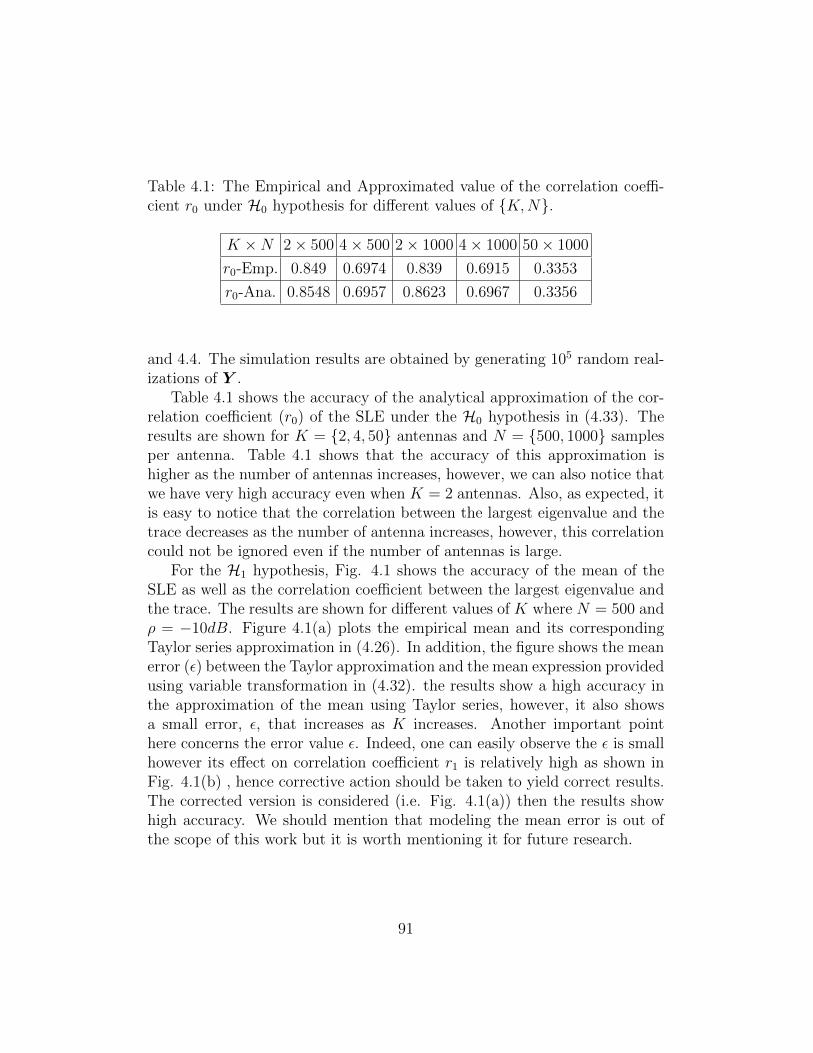
Table 4.1: The Empirical and Approximated value of the correlation coeffi-cient r0 under H0 hypothesis for different values of K,N.
K ×N 2× 500 4× 500 2× 1000 4× 1000 50× 1000
r0-Emp. 0.849 0.6974 0.839 0.6915 0.3353
r0-Ana. 0.8548 0.6957 0.8623 0.6967 0.3356
and 4.4. The simulation results are obtained by generating 105 random real-izations of Y .
Table 4.1 shows the accuracy of the analytical approximation of the cor-relation coefficient (r0) of the SLE under the H0 hypothesis in (4.33). Theresults are shown for K = 2, 4, 50 antennas and N = 500, 1000 samplesper antenna. Table 4.1 shows that the accuracy of this approximation ishigher as the number of antennas increases, however, we can also notice thatwe have very high accuracy even when K = 2 antennas. Also, as expected, itis easy to notice that the correlation between the largest eigenvalue and thetrace decreases as the number of antenna increases, however, this correlationcould not be ignored even if the number of antennas is large.
For the H1 hypothesis, Fig. 4.1 shows the accuracy of the mean of theSLE as well as the correlation coefficient between the largest eigenvalue andthe trace. The results are shown for different values of K where N = 500 andρ = −10dB. Figure 4.1(a) plots the empirical mean and its correspondingTaylor series approximation in (4.26). In addition, the figure shows the meanerror (ε) between the Taylor approximation and the mean expression providedusing variable transformation in (4.32). the results show a high accuracy inthe approximation of the mean using Taylor series, however, it also showsa small error, ε, that increases as K increases. Another important pointhere concerns the error value ε. Indeed, one can easily observe the ε is smallhowever its effect on correlation coefficient r1 is relatively high as shown inFig. 4.1(b) , hence corrective action should be taken to yield correct results.The corrected version is considered (i.e. Fig. 4.1(a)) then the results showhigh accuracy. We should mention that modeling the mean error is out ofthe scope of this work but it is worth mentioning it for future research.
91
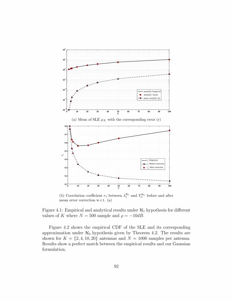
0 10 20 30 40 50 60 70 80 90 10010
−4
10−3
10−2
10−1
100
101
102
K
mean(X): Empirical
mean(X): Taylor
mean−error(X) (ε)
(a) Mean of SLE µX with the corresponding error (ε)
0 10 20 30 40 50 60 70 80 90 1000.1
0.2
0.3
0.4
0.5
0.6
0.7
0.8
K
r 1
r1: Empirical
r1: Before correction
r1: After correction
(b) Correlation coefficient r1 between λH11 and TH1
n before and aftermean error correction w.r.t. (a)
Figure 4.1: Empirical and analytical results underH1 hypothesis for differentvalues of K where N = 500 sample and ρ = −10dB.
Figure 4.2 shows the empirical CDF of the SLE and its correspondingapproximation under H0 hypothesis given by Theorem 4.2. The results areshown for K = 2, 4, 10, 20 antennas and N = 1000 samples per antenna.Results show a perfect match between the empirical results and our Gaussianformulation.
92
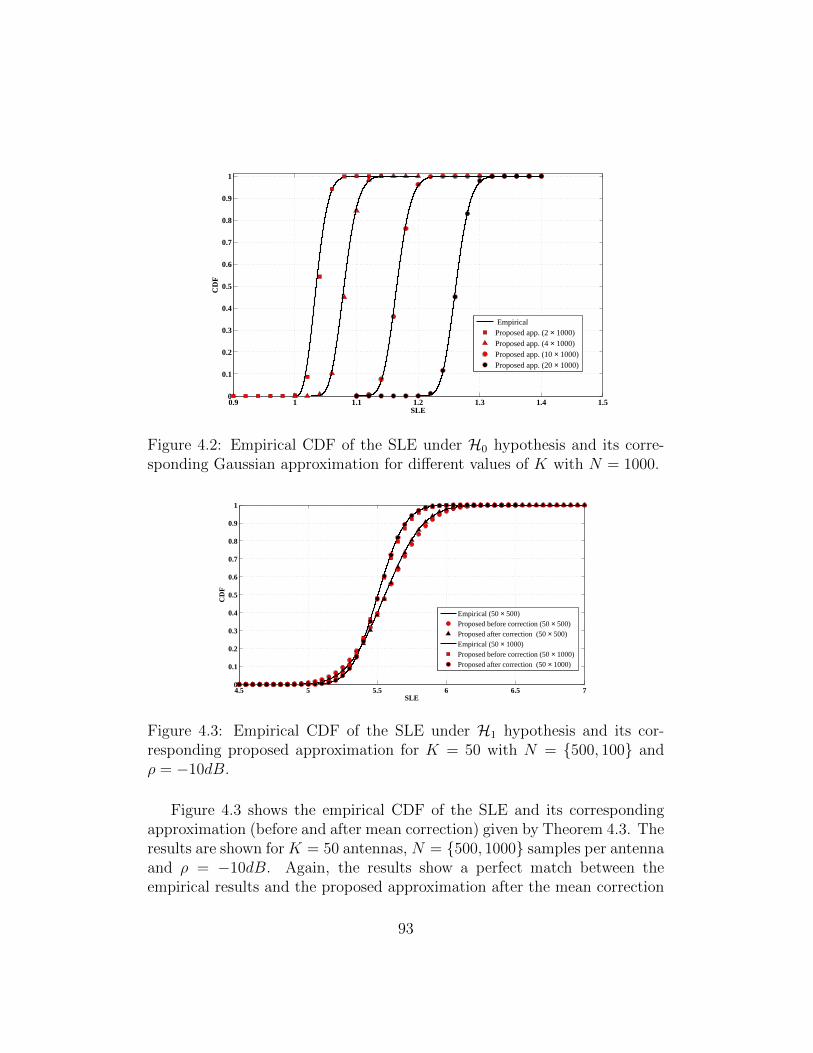
0.9 1 1.1 1.2 1.3 1.4 1.50
0.1
0.2
0.3
0.4
0.5
0.6
0.7
0.8
0.9
1
SLE
CD
F
EmpiricalProposed app. (2 × 1000)Proposed app. (4 × 1000)Proposed app. (10 × 1000)Proposed app. (20 × 1000)
Figure 4.2: Empirical CDF of the SLE under H0 hypothesis and its corre-sponding Gaussian approximation for different values of K with N = 1000.
4.5 5 5.5 6 6.5 70
0.1
0.2
0.3
0.4
0.5
0.6
0.7
0.8
0.9
1
SLE
CD
F
Empirical (50 × 500)Proposed before correction (50 × 500)Proposed after correction (50 × 500)Empirical (50 × 1000)Proposed before correction (50 × 1000)Proposed after correction (50 × 1000)
Figure 4.3: Empirical CDF of the SLE under H1 hypothesis and its cor-responding proposed approximation for K = 50 with N = 500, 100 andρ = −10dB.
Figure 4.3 shows the empirical CDF of the SLE and its correspondingapproximation (before and after mean correction) given by Theorem 4.3. Theresults are shown for K = 50 antennas, N = 500, 1000 samples per antennaand ρ = −10dB. Again, the results show a perfect match between theempirical results and the proposed approximation after the mean correction
93
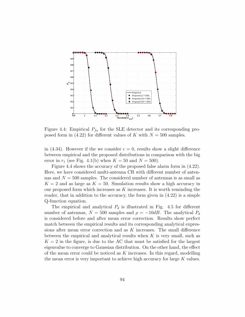
0.9 1 1.1 1.2 1.3 1.4 1.5 1.6 1.7 1.80
0.1
0.2
0.3
0.4
0.5
0.6
0.7
0.8
0.9
1
Threshold (λSLE
)
Pfa
EmpiricalProposed (2 × 500)Proposed (10 × 500)Proposed (50 × 500)
Figure 4.4: Empirical Pfa for the SLE detector and its corresponding pro-posed form in (4.22) for different values of K with N = 500 samples.
in (4.34). However if the we consider ε = 0, results show a slight differencebetween empirical and the proposed distributions in comparison with the bigerror in r1 (see Fig. 4.1(b) when K = 50 and N = 500).
Figure 4.4 shows the accuracy of the proposed false alarm form in (4.22).Here, we have considered multi-antenna CR with different number of anten-nas and N = 500 samples. The considered number of antennas is as small asK = 2 and as large as K = 50. Simulation results show a high accuracy inour proposed form which increases as K increases. It is worth reminding thereader, that in addition to the accuracy, the form given in (4.22) is a simpleQ-function equation.
The empirical and analytical Pd is illustrated in Fig. 4.5 for differentnumber of antennas, N = 500 samples and ρ = −10dB. The analytical Pdis considered before and after mean error correction. Results show perfectmatch between the empirical results and its corresponding analytical expres-sions after mean error correction and as K increases. The small differencebetween the empirical and analytical results when K is very small, such asK = 2 in the figure, is due to the AC that must be satisfied for the largesteigenvalue to converge to Gaussian distribution. On the other hand, the effectof the mean error could be noticed as K increases. In this regard, modellingthe mean error is very important to achieve high accuracy for large K values.
94
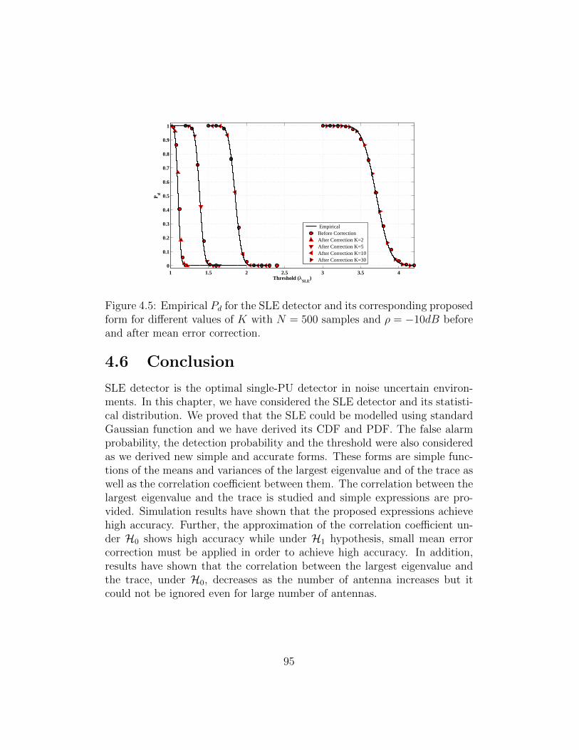
1 1.5 2 2.5 3 3.5 40
0.1
0.2
0.3
0.4
0.5
0.6
0.7
0.8
0.9
1
Threshold (λSLE
)
Pd
EmpiricalBefore CorrectionAfter Correction K=2After Correction K=5After Correction K=10After Correction K=30
Figure 4.5: Empirical Pd for the SLE detector and its corresponding proposedform for different values of K with N = 500 samples and ρ = −10dB beforeand after mean error correction.
4.6 Conclusion
SLE detector is the optimal single-PU detector in noise uncertain environ-ments. In this chapter, we have considered the SLE detector and its statisti-cal distribution. We proved that the SLE could be modelled using standardGaussian function and we have derived its CDF and PDF. The false alarmprobability, the detection probability and the threshold were also consideredas we derived new simple and accurate forms. These forms are simple func-tions of the means and variances of the largest eigenvalue and of the trace aswell as the correlation coefficient between them. The correlation between thelargest eigenvalue and the trace is studied and simple expressions are pro-vided. Simulation results have shown that the proposed expressions achievehigh accuracy. Further, the approximation of the correlation coefficient un-der H0 shows high accuracy while under H1 hypothesis, small mean errorcorrection must be applied in order to achieve high accuracy. In addition,results have shown that the correlation between the largest eigenvalue andthe trace, under H0, decreases as the number of antenna increases but itcould not be ignored even for large number of antennas.
95
Chapter 5
Multi-Antenna Based
Spectrum Sensing:
Approaching Massive MIMOs
This chapter considers a cognitive radio (CR) equipped with massive MIMOtechnology that uses the EBD for SS. Sec. 5.1 introduces the problem anddiscusses the different scenarios and cases considered in this chapter. TheLE detector in the finite case is considered in Sec. 5.2 where we derive exactexpressions and approximated ones. The full exploitation of the antennasare discussed in 5.3 and the partial exploitation is discussed in 5.4 for LE,SCN and SLE detectors. Finally, the conclusion is derived in Sec. 5.6.
5.1 Introduction
The fifth generation (5G) of mobile network is expected to be deployed by2020. As 5G has to accommodate new demands and high data-rates growingat an unprecedented pace, a large amount of radio frequency resources isstill under-utilized. For instance, by exploiting the spatial domain, massiveMIMO is introduced to increase the network capacity for the next generationwireless systems [209–211]. A massive MIMO system uses up to few hundredof antennas to gain all the benefits of the conventional MIMO but on a muchlarger scale. As such, CR could be combined with massive MIMO throughthe additional degree of freedom offered by the large number of antennas
96

to identify the unused channels while achieving a significant increase in theperformance of the SS detector. In this regard, it is very likely to considerthe EBD to detect the spectrum holes in CR with massive MIMO technology.
In fact, a CR system with massive MIMO technology could use all anten-nas for the SS and achieve an enormous performance enhancement. Howeverit might be enough to use a fewer number of antennas for the sensing processand thus define a more efficient way for antenna exploitation. In this regard,two scenarios could be considered:
1. Full antenna exploitation scenario: Therein, the CR module may use allof its antennas in the SS and hence may reduce the number of samplesrequired for SS.
2. Partial antenna exploitation scenario: In this scenario, the CR may fixcertain number of antennas to a given SS process and use the othersfor other purposes (such as transmission) or it may dynamically changethe number of antennas K and/or the number of samples N accordingto predefined performance and also use the rest for other purposes.
In this chapter, the EBD is used due to its importance in multi-antennaSS. Specifically, we will consider the LE detector which is proved to be theoptimal if noise power is perfectly known. Accordingly, we suppose that thenoise power is perfectly known. Moreover, LE detector could be evaluatedwithout the need of the EVD and thus avoid some computational complexityby using the power method. From here, let us differentiate between thefollowing cases:
Case 1: Finite K and finite N : In this case, the CR module utilizes a smallfinite number of antennas K and a relatively small finite number ofsamples N for partial exploitation.
Case 2: Finite K and asymptotic N : Here, the CR module utilizes a finitenumber of antennas K and a relatively large number of samples N forpartial exploitation.
Case 3: Asymptotic K and asymptotic N : In this case, the CR uses a Largenumber of antennas K and a large number of samples N such thatN > K for full antenna exploitation.
It is worth mentioning that in case 1, the performance analysis and thedecision threshold selection could not rely on any asymptotic approximations.
97
Indeed, the use of finite RMT analysis to study the statistics of the LEdetector is the best solution. On the other hand, in cases 2 and 3 the use ofapproximations related to large number of antenna and/or large number ofsamples are extremely beneficial.
On the other hand, when noise power is not perfectly known then theSCN and SLE detectors discussed in previous chapters could be considered.Accordingly, an extension to the SCN and SLE detectors is done by usingthe results derived in Chapters 3 and 4. The dynamic antenna exploitationcase is considered for the mentioned three detectors (i.e. LE, SCN and SLEdetectors) and the minimum requirements needed to achieve a target perfor-mance is considered. Accordingly, a comparison between these detectors isprovided in terms of sensing performance and minimum requirements.
5.2 LE Detector in Finite Case: Small num-
ber of antennas and samples
In this section, we will consider the LE detector in the finite case (i.e. Case1). The CDF of the LE decision metric is considered since it is directly re-lated to the performance probabilities as provided by (2.6), (2.7) and (2.8).Consequently, we show that the computational complexity of these expres-sions increases as K or N increases. Moreover, it is difficult to derive athreshold using such expressions. Accordingly and since we are dealing withthe extreme eigenvalue, we propose to approximate the distribution of theLE decision metric using the GEV approximation described in AppendixC. Based on this approximation, a simple expression of the decision thresh-old is provided by which a CR system using small number of antennas andrelatively small number of samples for SS can compute the threshold valueonline.
5.2.1 LE Detector in Finite Case
The Largest eigenvalue detector is a semi-blind detector since it requires theknowledge of noise power, however, if perfect knowledge is available thenLE is the optimal detector [42]. LE is the largest eigenvalue of the samplecovariance matrix and its exact distribution is derived in literature (see, forinstance, [178, 212]) in the form of matrix determinant whose complexityincreases as the number of antenna increases. Asymptotically, LE is proved
98
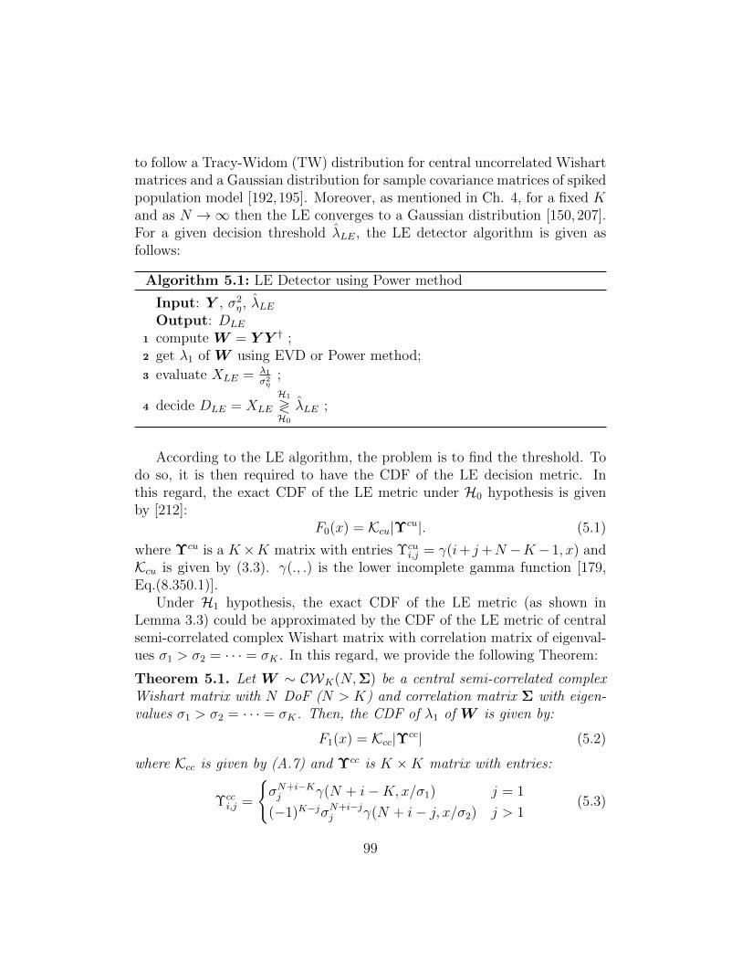
to follow a Tracy-Widom (TW) distribution for central uncorrelated Wishartmatrices and a Gaussian distribution for sample covariance matrices of spikedpopulation model [192,195]. Moreover, as mentioned in Ch. 4, for a fixed Kand as N →∞ then the LE converges to a Gaussian distribution [150,207].For a given decision threshold λLE, the LE detector algorithm is given asfollows:
Algorithm 5.1: LE Detector using Power method
Input: Y , σ2η, λLE
Output: DLE
1 compute W = Y Y † ;2 get λ1 of W using EVD or Power method;
3 evaluate XLE = λ1
σ2η
;
4 decide DLE = XLE
H1
≷H0
λLE ;
According to the LE algorithm, the problem is to find the threshold. Todo so, it is then required to have the CDF of the LE decision metric. Inthis regard, the exact CDF of the LE metric under H0 hypothesis is givenby [212]:
F0(x) = Kcu|Υcu|. (5.1)
where Υcu is a K×K matrix with entries Υcui,j = γ(i+ j+N −K− 1, x) and
Kcu is given by (3.3). γ(., .) is the lower incomplete gamma function [179,Eq.(8.350.1)].
Under H1 hypothesis, the exact CDF of the LE metric (as shown inLemma 3.3) could be approximated by the CDF of the LE metric of centralsemi-correlated complex Wishart matrix with correlation matrix of eigenval-ues σ1 > σ2 = · · · = σK . In this regard, we provide the following Theorem:
Theorem 5.1. Let W ∼ CWK(N,Σ) be a central semi-correlated complexWishart matrix with N DoF (N > K) and correlation matrix Σ with eigen-values σ1 > σ2 = · · · = σK. Then, the CDF of λ1 of W is given by:
F1(x) = Kcc|Υcc| (5.2)
where Kcc is given by (A.7) and Υcc is K ×K matrix with entries:
Υcci,j =
σN+i−Kj γ(N + i−K, x/σ1) j = 1
(−1)K−jσN+i−jj γ(N + i− j, x/σ2) j > 1
(5.3)
99
Proof. Starting from the joint distribution in (A.5), the CDF of the largesteigenvalue, using [176, Corollary 2], is given by:
F1(x) =
∫ x
0
· · ·∫ x
0
f(λ)dλ (5.4)
= Kcc∣∣∣∣∫ x
0
vi(u)ej(u)uN−Kdu
∣∣∣∣i,j=1,··· ,K
, (5.5)
then, the integral of (5.5) is evaluated using [179, Eq. 3.351.1].
Note that γ(n, x) = (n − 1)!e−x∑n−1
m=0xm
m![179], then the evaluation of
these exact CDFs is more complicated as K or N increases. However, thetarget is to find a simple threshold form which is not straightforward sinceit requires the inverse of the CDF function. Next, we show that the LEdistribution could be perfectly approximated using the GEV distributionand thus a simple threshold form could be derived.
5.2.2 Approximating LE
Herein, the approximation of the LE distribution is considered. First, themoments of the LE are derived and then an approximation of the LE distri-bution with the GEV distribution will follow using Lemma C.1. We shouldmention that this approximation is feasible if the moments are derived. Thus,the exact form of the p-th moment of the LE under hypothesis H0 is providedby the following Theorem.
Theorem 5.2. Let W ∼ CWK(N, σ2ηIK) be a central uncorrelated complex
Wishart matrix with N DoF and correlation matrix σ2ηIK. Then, the p-th
moment of the LE of W is given by:
M(p) = pKcu∑δ∈P0
sgn(δ)K∏i=1
(δ(i) + i+N −K − 2)!
×∑s∈S∗0
(−1)|s|+1(Σs+ p− 1)!
Πs! · |s|Σs+p(5.6)
with P0 is the set of all possible permutations of the vector [1, · · · , K] and thesum is taken over all possible permutations. sgn(δ) is the permutation signof the permuted vector δ. S∗0 is the set of all subsets of the vector [l1, · · · , lK ]
100
and the sum is taken over all possible subsets except the null subset such
that∑s∈S∗0
=∑L1
l1· · ·∑L|s|
l|s|with |s| is the cardinality of the subset s and
Lj = δ(j) + j +N −K − 2.
Proof. See App. A.5.
Under H1 hypothesis and following the results in Ch. 3, the use of themoments of the central semi-correlated Wishart matrices provide good ap-proximation for the LE. Hence, the exact form of the p-th moment of thelargest eigenvalue of the central semi-correlated Wishart matrices of spikedpopulation is provided by the following Theorem:
Theorem 5.3. Let W ∼ CWK(N,Σ) be a central semi-correlated complexWishart matrix with N DoF (N > K) and correlation matrix Σ with eigen-values σ1 > σ2 = · · · = σK. Then, the p-th moment of λ1 of W is givenby:
M(p) = pK′cu∑δ∈P0
sgn(δ)K∏i=1
(N + δ(i)− bi,K − 1)!
σbi,K−δ(i)−Ni
×∑s∈S∗0
(−1)|s|+1(Σs+ p− 1)!
Πs! · Πσss · |Σ 1σs|Σs+p
, (5.7)
with K′cu is a modified normalization constant as follows:
K′cc =(−1)
(K−1)(K−2)2 σK−N−1
1 σ(N−1)(1−K)2
ΓK(N)ΓK−1(K − 1)(σ2 − σ1)K−1, (5.8)
and we define bn,m as:
bn,m =
m n = 1
n n 6= 1(5.9)
Proof. See App. A.5.
Same as for the CDF case, the p-th moment of the LE metric is providedby (5.7) after the normalization of W by σ2
η. Now by exploiting the mo-ments of the LE given by Theorems 5.2 and 5.3, we can approximate the LEdistribution by the GEV distribution as given by the following proposition.
101
Proposition 5.1. The CDF and PDF of the LE, under hypotheses H0 andH1, can be accurately approximated by:
F (x; θ, β, ξ) = e−(1+(x−θβ
)ξ)−1/ξ
(5.10)
f(x; θ, β, ξ) =1
β(1 + (
x− θβ
)ξ)−1ξ−1e−(1+(x−θ
β)ξ)−1/ξ
(5.11)
where the shape, scale and location parameters are defined by (3.43), (3.44)and (3.45) with the mean, variance and skewness of LE given by:
µLE = M(1) (5.12)
σ2LE = M(2)− µ2
LE (5.13)
SLE =M(3)− 3M(2)µLE + 2µ3
LE
σ3/2LE
(5.14)
with M(p) is the p-th moments of the LE given by Theorems 5.2 and 5.3 forH0 and H1 cases respectively.
Using (5.10), the performance probabilities and the decision thresholdcould be derived as in Sec. 3.3.4. It should be noted that the computationalcomplexity of the moments of the LE in (5.6) and (5.7) is higher than thatof the CDF in (5.1) and (5.2). This is obvious since the determinant couldbe calculated using LU decomposition algorithm (O(K3)) and we use theLeibniz formula which requires n!n operations. However, as mentioned inCh. 3, this approximation only requires the values of the location, scale andshape parameters of the GEV distribution that could be computed off-line.
We should here mention that the approximation of the LE using GEV isfor any K and N (i.e. finite and asymptotic). However, in the particular casewhen K is finite and N asymptotic, the LE could be modelled as a GaussianRV, as mentioned in Ch. 4, which is simple and useful as discussed later inthis chapter.
102
5.3 LE Detector with Asymptotic Regime:
Full antenna exploitation
In this scenario, the CR will use all of its antennas for the SS process. Ac-cordingly, recall the asymptotic and critical conditions as follows:
AC : (K,N)→∞ with K/N → c ∈ (0, 1), (5.15)
CC : ρ > ρc =1√KN
, (5.16)
Again, in asymptotic regime, the problem turns out to find the distribu-tion and the threshold. By considering the AC, then under H0 hypothesis,LE, properly centered and scaled, follows a TW distribution of order 2 (TW2)as follows [192]:
LE ′ =LE − a1(K,N)
b1(K,N)∼ TW2, (5.17)
where a1(K,N) and b1(K,N) are respectively the centering and scaling co-efficients defined by (3.52) and (3.53).
The CDF of the TW2, first considered in [186], is given by (5.18) whereq(x) is the solution to the Painleve II differential equation q′′(x) = xq(x) +2q3(x) satisfying the boundary condition q(x) ∼ Ai(x) as x → ∞ whereAi(x) is the Airy function.
FTW2(y) = e−∫∞y (x−y)q2(x)dx. (5.18)
On the other hand, if both AC and CC are met then LE under H1 hy-pothesis and using Lemma 3.3 follows a normal distribution as follows [195]:
P (LE − a3(K,N,σ)√
b3(K,N,σ)≤ x) =
1√2π
∫ x
−∞e−
u2
2 du, (5.19)
with a3(K,N,σ) and b3(K,N,σ) are defined in (3.64) and (3.65) respectivelywith σ2
η = 1.It is worth mentioning that the TW2 distribution could not be evaluated
numerically online. In fact, the cognitive radio system needs to evaluate thethreshold which requires the inverse of the CDF. In the next subsection, weapproximate the LE distribution with the GEV distribution in the asymptoticregime.
103
5.3.1 Approximating LE in asymptotic regime
Under H0 hypothesis and when AC is satisfied, the distribution of the LEmetric could be approximated through GEV using the mean, the variance andthe skewness provided in (3.57), (3.58) and (3.59) respectively. Accordingly,we give the following proposition:
Proposition 5.2. Let N and K obey AC in (5.15), then the CDF and PDFof the LE under H0 hypothesis can be accurately approximated by (5.10) and(5.11) respectively. The shape, scale and location parameters are defined by(3.43), (3.44) and (3.45) where the mean, the variance and the skewness ofLE are given by (3.57), (3.58) and (3.59) respectively.
It follows from Proposition 5.2 that the GEV approximation could alsobe used to approximate the TW2 distribution by considering the mean, thevariance and the skewness of TW2 given by µTW2 = −1.7710868074, σ2
TW2 =0.8131947928 and STW2 = 0.2240842036 respectively.
Based on Proposition 5.2, the threshold expression is simple and have thesame form of (3.95) for CFAR. On the other hand under H1 hypothesis, thedistribution is Gaussian and it is indeed simple and any approximation inthis case is useless.
5.4 Partial Exploitation of Massive MIMO
antennas
This scenario could be decomposed into two different options; The first isthe fixed number of antenna approach where the CR will fix a predefinednumber of antennas for the SS and thus uses the rest for other purposesas it will be discussed in this section. The other approach is the dynamicapproach in which the CR does not fix a predefined number of antennas butit dynamically allocates a certain number of antennas for SS according tocertain constraints such as a target performance. The rest of the antennas isused for other purposes.
The division in this case into approaches could be simply justified bythe simple fact that a tradeoff between SS performance and exploitation ofavailable of antennas for other use could exist. This depends on the differentmetrics and outcomes expected in this case. For instance, fixing predefinednumber of antennas for the SS or knowing the minimum number of antennas
104

necessary to reach a prescribed performance within a given time has manyadvantages such as:
• Sensing multi-channels simultaneously: in this case, the antennas areclustered and each cluster of antennas is ordered to sense certain chan-nel and/or certain direction. Accordingly, several spectrum holes couldbe found at the same time which results in a more efficient utiliza-tion of the spectrum bands. Moreover, several techniques have beenproposed in literature to sense a wide-band channel such as the filter-bank, compressive sensing, wavelet decomposition as mentioned in Ch.2. Alternatively, massive MIMO could be used to sense a wide-bandchannel by dedicating the clusters to sense several narrow-band chan-nels simultaneously.
• Sense and transmit simultaneously: conventional SS could be eitherdone in a periodic sensing approach or in a simultaneous sensing andtransmission approach. In periodic sensing, the CR operates in a time-slots model where it senses for a short time duration and transmits datain the remaining time of total frame duration [213]. On the other hand,simultaneous sensing and transmission approach could be considered asa full duplex approach in which two RF chains are required at the CRreceiver [214]. Likewise, the CR could maintain a set antennas for SSand the others for the transmission in a full duplex scenario.
• Green radio: green radio concept has received a great attention in re-cent years. It is one of the most important considerations in the presentscenario of global warming. From an energy efficiency perspective, itmakes sense to put inactive antenna elements into sleep mode and thusreduce energy consumption [215].
• Reduce the sensing time: sensing time is the time required for the CRto make a decision. It indeed includes the required sampling durationand the time the sensing algorithm needs to make a decision. Accord-ingly, the full antenna exploitation scenario may not be the optimal forsensing time reduction. Indeed, if a trade-off between the complexity ofthe algorithm and the required number of samples to make a decisionis done this may decrease the total sensing time.
• Increase system throughput: In general, using some or all of thesemethods, i.e. sense multi-channels simultaneously, sense and transmit
105
simultaneously and reducing the sensing time, would increase the totalsystem throughput.
Consequently, the use of a fixed number or dynamic number of antennasfor SS is extremely important for CR with massive MIMO technology. Infixed number case, the CR may define any number of antenna K and samplesN for SS. Accordingly, and based on our derivations for LE, SLE and SCNdetector through this thesis, the threshold could be computed according tomaintain a CFAR or an optimized threshold could be used as to minimize thetotal error probabilities. The threshold optimization criteria is considered forthe LE detector in Sec. 5.4.2. On the other hand, the minimum number ofantennas and/or the minimum number of samples required to reach a targetperformance is very important for the dynamic approach. These values aredirectly related to the statistics of the SS decision metric being used and theenvironmental information. This is considered in Sec. 5.4.3 while using theLE detector and in Sec. 5.4.4 for the SCN and SLE detectors.
5.4.1 Performance Probabilities
To model the system, we should first define the performance probabilities ofthe detector used. In the partial antenna exploitation scenario, we considerthe following:
• Fixed number of antenna approach: in this case, the CR will use certainfixed number K and N > K. If K is large, then N is obviouslylarge and hence the results of asymptotic regime, in previous section,could be applied. On the other hand, if K is small, then N may berelatively small and hence the results of finite case in Sec. 5.2 areapplied. However, it is more likely that N will be relatively large.
• Dynamic number of antenna approach: here, the CR will use dynamicnumber of antenna K and N > K. If K is large, then N is obviouslylarge and the asymptotic results are applied. Also, if K is small and Nis relatively small then the results of finite case are applied. However,it is more likely to have certain number K and relatively large N .
Consequently, we will consider the case in which K is finite and N isrelatively large which is more practical. Hence the LE metric could be mod-eled as Gaussian RV under H0 hypothesis. Under H1 hypothesis, results
106
in [150] shows that LE metric could be approximated by Gaussian even ifK is small and N is relatively large and CC is satisfied. Accordingly, if wedenote the decision threshold of the LE detector by λLE, then Pfa, Pd andPmd are expressed as follows:
Pfa = 1− Φ(λLE − µ0
σ0
) (5.20)
Pmd = 1− Pd = Φ(λLE − µ1
σ1
) (5.21)
where Φ(.) is the CDF of the standard normal distribution; µ0, σ0 are themean and the standard deviation of the LE metric under H0 hypothesis andare given by (5.22) and (5.23) (recalled from Ch. 3); µ1, σ1 are the mean andthe standard deviation of the LE metric under H1 hypothesis and are givenby (5.24) and (5.25) (recalled from Ch. 3).
µ0 = b1(K,N)µTW2 + a1(K,N), (5.22)
σ20 = b2
1(K,N)σ2TW2, (5.23)
µ1 = σ1(N +K
σ1 − 1), (5.24)
σ21 = σ2
1(N − K
(σ1 − 1)2), (5.25)
where µTW2 = −1.7710868074, σ2TW2 = 0.8131947928 and
a1(K,N) = (√K +
√N)2, (5.26)
b1(K,N) = (√K +
√N)(K−1/2 +N−1/2)
13 . (5.27)
5.4.2 Optimal Threshold
The performance probabilities depend on the decision threshold (λLE), andhence it is necessary to choose an appropriate value based on system require-ments. The typical approach for setting the threshold is given by the CFARstrategy in which the threshold is chosen in order to guarantee a target false-alarm rate (Pfa). Hence, for finite K and relatively large N and based onthe CFAR scenario, the decision threshold is expressed using the inverse ofPfa as follows:
λLE = µ0 + σ0Φ−1(1− Pfa) (5.28)
107
It is worth mentioning that the threshold for other cases (i.e. asymptoticand finite) is previously derived and given by (3.95). Another thresholdoptimization approach would be to minimize the total error probability of thesystem. Accordingly, the optimized threshold could be expressed as follows:
λLE = argminλLE
(p0Pfa + p1Pmd) (5.29)
where p0 and p1 are weighting coefficients that are chosen according to sys-tem priority. To solve this minimization problem, one can simply take thederivative equals to zero and the second derivative positive (i.e. concave).One can choose p0 = 0 or p1 = 0 to minimize one of the error probabili-ties. However, it is typical to choose p0 = p1 = 0.5 to minimize the sum ofthe error probabilities. Then λLE should be selected such that it minimizesPfa + Pmd, i.e. its derivative equal to zero such that:
(1
2σ20
− 1
2σ21
)λ2LE + (
µ1
σ21
− µ0
σ20
)λLE + (µ2
0
2σ20
− µ21
2σ21
− ln(σ1
σ0
)) = 0 (5.30)
and finally the optimal threshold is given by:
λLE =
µ1σ20 − µ0σ
21 +
√σ2
0σ21
((µ0 − µ1)2 − 2(σ2
0 − σ21)ln(σ1
σ0))
σ20 − σ2
1
(5.31)
The same derivation procedure could be done for any value p0 and p1. Theoptimal threshold in (5.31) requires the knowledge of the SNR value. It couldbe used in any of the scenarios to minimize the error probabilities. However,in the dynamic case, i.e. when K and/or N are to be selected dynamically,the designer should set up the target Pfa and Pmd to be obtained while theoptimization will consist in finding the minimal K and N . Accordingly, wechoose a fixed (Pfa, Pd) performance to evaluate the required K and N toachieve this performance. This will be discussed next.
5.4.3 Minimum Requirements
For a target (Pfa, Pd) and at a given SNR, the CR system should optimizecertain number of antennas for a certain number of samples. By eliminatingλLE from Pfa and Pd in (5.20) and (5.21) respectively, one can solve for K(or N) the following equation:
σ0Φ−1(1− Pfa)− σ1Φ−1(1− Pd) + µ0 − µ1 = 0 (5.32)
108

Now, let us substitute µ0, µ1, σ0 and σ1 to get a single equation involving theparameters: K, N , Pfa, Pd and ρ. Hence, at a certain SNR value and for a
target detection performance (Pfa, Pd) the system can dynamically choose thecouple (K,N) that most enhances its global performance (i.e. throughput,power saving etc.). In is worth mentioning that finding a general solution for(5.32) is not straightforward and thus we solve for numerical values. Considerthe following example:
Example 1: Consider the following example, Pfa = 0.1, Pd = 0.9 andρ = −15dB, then we get Tables 5.1 and 5.2.
Table 5.1: Required K for a given N in Example 1.
N 200 300 350 400 450 500 600 1000K 14 10 8 8 7 6 5 4
Table 5.2: Required N for a given K in Example 1.
K 20 18 15 10 8N 132 147 177 273 349
Table 5.1 shows different values of N and its corresponding required num-ber of antennas K that should be involved in the sensing process to achievethe performance illustrated in Example 1. On the other hand, Table 5.2shows different values of K and its corresponding required number of sam-ples N that should be acquired by each antenna in the sensing process toachieve the considered performance. It is worth mentioning that the valuesof K and N evaluated using (5.32) are real valued numbers and thus arerounded to +∞. Consequently, for a target performance as illustrated inExample 1 it is enough for a CR to use K = 8 and N = 350. However, usinga greater number of antennas is inefficient and a waste of resources.
The system may also be expected to have dynamic behaviour in case ofthe change of the SNR values. This could be also achieved using (5.32). Thiskind of dynamical behaviour is extremely important to any multi-antennasystem. This will be considered in the simulations.
109
5.4.4 Extension to SCN and SLE
In this subsection, we use the results provided in Chapters 3 and 4 to extendthis work for both SCN and SLE detectors. Let us consider the SCN detectorand by eliminating λSCN from both (3.93) and (3.94) we get:
θ0−β0
ξ0
− θ1 +β1
ξ1
+β0
ξ0
[− ln(1− Pfa)
]−ξ0 − β1
ξ1
[− ln(1− Pd)
]−ξ1 = 0 (5.33)
where Pfa and Pd are target false-alarm and detection probabilities; θi, βiand ξi are the location, scale and shape parameters of the GEV distributionwhere i = 0 refers to H0 hypothesis and i = 1 refers to H1 hypothesis. Theirexpressions are provided by Theorems 3.2 and 3.3.
For the SLE detector, the probability of detection could be derived in asimilar manner used for the derivation of Pfa in Sec. 4.3.3. Accordingly, byeliminating λSLE from the performance probabilities we get:
µH012 −∆2r0σ
H012
µ2
TH0n
−∆2σ2
TH0n
− µH112 − Λ2r1σ
H112
µ2
TH1n
− Λ2σ2
TH1n
+∆√mH0v − 2r0µ
H012 σ
H012 + ∆2[σH0
12 ]2(r20 − 1)
µ2
TH0n
−∆2σ2
TH0n
−Λ√mH1v − 2r1µ
H112 σ
H112 + Λ2[σH1
12 ]2(r21 − 1)
µ2
TH1n
− Λ2σ2
TH1n
= 0 (5.34)
where ∆ = Q−1(Pfa) and Λ = Q−1(Pd); the expressions of the parameters in(5.34) are provided in Ch. 4.
Similar to the LE detector case, using (5.33) and (5.34) we can determinethe minimum requirements of the system that could be used to achieve targetperformance.
5.5 Simulation and Discussion
In this section, we verify the analytical derivation results through Monte-Carlo simulations. We validate the theoretical analysis presented in sections5.2, 5.3 and 5.4. The simulation results are obtained by generating 105
random realizations of Y . In addition, we compare the results of differentscenarios of antenna exploitation for different considered detectors. More-over, a comparison between the LE, SCN and SLE detectors is consideredfrom the performance perspective and the minimum requirements needed toachieve target performance.
110
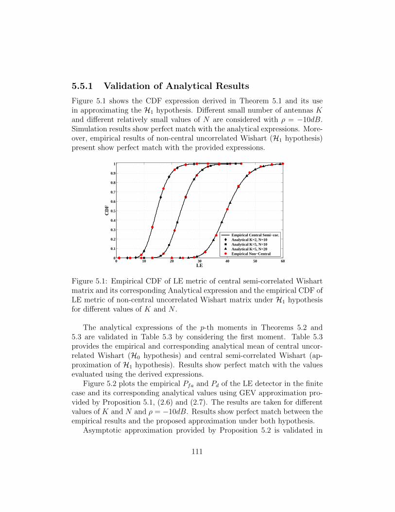
5.5.1 Validation of Analytical Results
Figure 5.1 shows the CDF expression derived in Theorem 5.1 and its usein approximating the H1 hypothesis. Different small number of antennas Kand different relatively small values of N are considered with ρ = −10dB.Simulation results show perfect match with the analytical expressions. More-over, empirical results of non-central uncorrelated Wishart (H1 hypothesis)present show perfect match with the provided expressions.
0 10 20 30 40 50 600
0.1
0.2
0.3
0.4
0.5
0.6
0.7
0.8
0.9
1
LE
CD
F
Empirical Central Semi−cor. Analytical K=2, N=10 Analytical K=5, N=10 Analytical K=5, N=20 Empirical Non−Central
Figure 5.1: Empirical CDF of LE metric of central semi-correlated Wishartmatrix and its corresponding Analytical expression and the empirical CDF ofLE metric of non-central uncorrelated Wishart matrix under H1 hypothesisfor different values of K and N .
The analytical expressions of the p-th moments in Theorems 5.2 and5.3 are validated in Table 5.3 by considering the first moment. Table 5.3provides the empirical and corresponding analytical mean of central uncor-related Wishart (H0 hypothesis) and central semi-correlated Wishart (ap-proximation of H1 hypothesis). Results show perfect match with the valuesevaluated using the derived expressions.
Figure 5.2 plots the empirical Pfa and Pd of the LE detector in the finitecase and its corresponding analytical values using GEV approximation pro-vided by Proposition 5.1, (2.6) and (2.7). The results are taken for differentvalues of K and N and ρ = −10dB. Results show perfect match between theempirical results and the proposed approximation under both hypothesis.
Asymptotic approximation provided by Proposition 5.2 is validated in
111
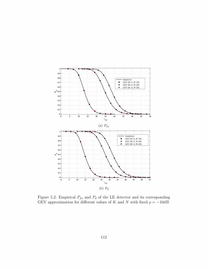
λLE
0 5 10 15 20 25 30 35 40 45 50
Pfa
0
0.1
0.2
0.3
0.4
0.5
0.6
0.7
0.8
0.9
1
Empirical GEV (K=2, N=10) GEV (K=2, N=20) GEV (K=3, N=20)
(a) Pfa
λLE
0 5 10 15 20 25 30 35 40 45 50 55
Pd
0
0.1
0.2
0.3
0.4
0.5
0.6
0.7
0.8
0.9
1
Analytical GEV (K=2, N=10) GEV (K=2, N=20) GEV (K=3, N=20)
(b) Pd
Figure 5.2: Empirical Pfa and Pd of the LE detector and its correspondingGEV approximation for different values of K and N with fixed ρ = −10dB.
112
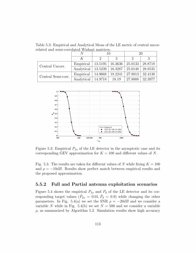
Table 5.3: Empirical and Analytical Mean of the LE metric of central uncor-related and semi-correlated Wishart matrices.
N 10 20
K 2 3 2 3
Central Uncorr.Empirical 13.5195 16.3636 25.0133 28.8718
Analytical 13.5239 16.3287 25.0148 28.8535
Central Semi-corr.Empirical 14.9668 18.2241 27.8013 32.4138
Analytical 14.9718 18.19 27.8008 32.3977
λLE
500 600 650-850 900 1000
Pfa
0
0.1
0.2
0.3
0.4
0.5
0.6
0.7
0.8
0.9
1
Empirical GEV (K=100, N=200) GEV (K=100, N=500)
Figure 5.3: Empirical Pfa of the LE detector in the asymptotic case and itscorresponding GEV approximation for K = 100 and different values of N .
Fig. 5.3. The results are taken for different values of N while fixing K = 100and ρ = −10dB. Results show perfect match between empirical results andthe proposed approximation.
5.5.2 Full and Partial antenna exploitation scenarios
Figure 5.4 shows the empirical Pfa and Pd of the LE detector and its cor-
responding target values (Pfa = 0.01, Pd = 0.9) while changing the otherparameters. In Fig. 5.4(a) we set the SNR ρ = −20dB and we consider avariable N while in Fig. 5.4(b) we set N = 500 and we consider a variableρ, as summarized by Algorithm 5.2. Simulation results show high accuracy
113
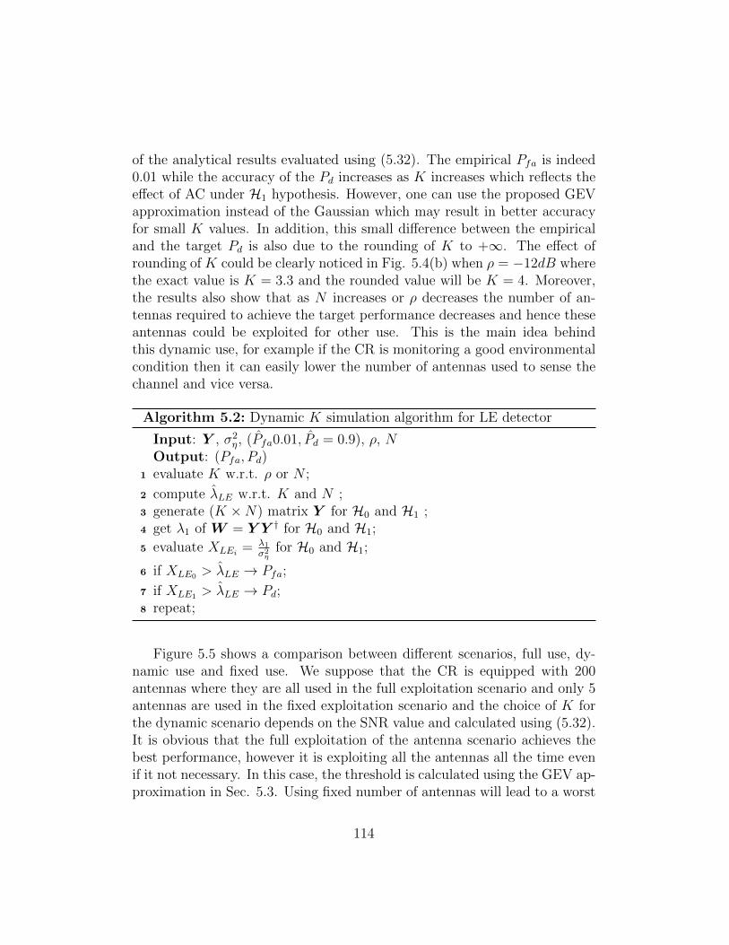
of the analytical results evaluated using (5.32). The empirical Pfa is indeed0.01 while the accuracy of the Pd increases as K increases which reflects theeffect of AC under H1 hypothesis. However, one can use the proposed GEVapproximation instead of the Gaussian which may result in better accuracyfor small K values. In addition, this small difference between the empiricaland the target Pd is also due to the rounding of K to +∞. The effect ofrounding of K could be clearly noticed in Fig. 5.4(b) when ρ = −12dB wherethe exact value is K = 3.3 and the rounded value will be K = 4. Moreover,the results also show that as N increases or ρ decreases the number of an-tennas required to achieve the target performance decreases and hence theseantennas could be exploited for other use. This is the main idea behindthis dynamic use, for example if the CR is monitoring a good environmentalcondition then it can easily lower the number of antennas used to sense thechannel and vice versa.
Algorithm 5.2: Dynamic K simulation algorithm for LE detector
Input: Y , σ2η, (Pfa0.01, Pd = 0.9), ρ, N
Output: (Pfa, Pd)1 evaluate K w.r.t. ρ or N ;
2 compute λLE w.r.t. K and N ;3 generate (K ×N) matrix Y for H0 and H1 ;4 get λ1 of W = Y Y † for H0 and H1;
5 evaluate XLEi = λ1
σ2η
for H0 and H1;
6 if XLE0 > λLE → Pfa;
7 if XLE1 > λLE → Pd;8 repeat;
Figure 5.5 shows a comparison between different scenarios, full use, dy-namic use and fixed use. We suppose that the CR is equipped with 200antennas where they are all used in the full exploitation scenario and only 5antennas are used in the fixed exploitation scenario and the choice of K forthe dynamic scenario depends on the SNR value and calculated using (5.32).It is obvious that the full exploitation of the antenna scenario achieves thebest performance, however it is exploiting all the antennas all the time evenif it not necessary. In this case, the threshold is calculated using the GEV ap-proximation in Sec. 5.3. Using fixed number of antennas will lead to a worst
114
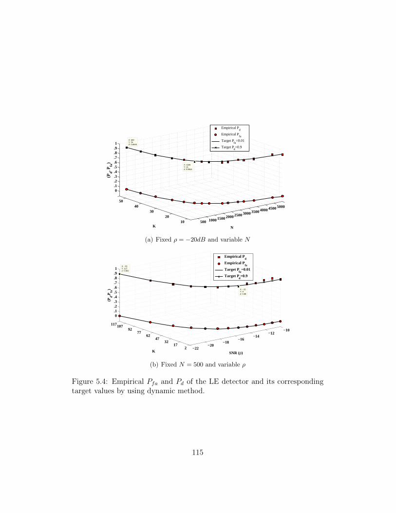
500 1000 1500 2000 2500 3000 3500 4000 4500 5000
1020
3040
50
0.1.2.3.4.5.6.7.8.91
N
X: 1500Y: 21Z: 0.8815
K
X: 500Y: 54Z: 0.8945
(Pd, P
fa)
Empirical Pd
Empirical Pfa
Target Pfa
=0.01
Target Pd=0.9
(a) Fixed ρ = −20dB and variable N
−22−20
−18−16
−14−12
−10
217
3247
6277
92107117
0.1.2.3.4.5.6.7.8.91
X: −15Y: 9Z: 0.88
SNR (ρ)K
X: −22Y: 117Z: 0.902
(Pd,P
fa)
Empirical Pd
Empirical Pfa
Target Pfa
=0.01
Target Pd=0.9
(b) Fixed N = 500 and variable ρ
Figure 5.4: Empirical Pfa and Pd of the LE detector and its correspondingtarget values by using dynamic method.
115
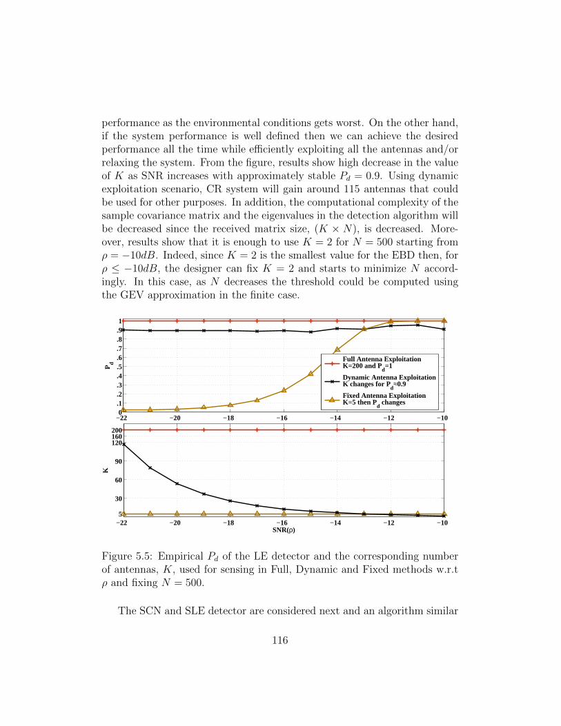
performance as the environmental conditions gets worst. On the other hand,if the system performance is well defined then we can achieve the desiredperformance all the time while efficiently exploiting all the antennas and/orrelaxing the system. From the figure, results show high decrease in the valueof K as SNR increases with approximately stable Pd = 0.9. Using dynamicexploitation scenario, CR system will gain around 115 antennas that couldbe used for other purposes. In addition, the computational complexity of thesample covariance matrix and the eigenvalues in the detection algorithm willbe decreased since the received matrix size, (K × N), is decreased. More-over, results show that it is enough to use K = 2 for N = 500 starting fromρ = −10dB. Indeed, since K = 2 is the smallest value for the EBD then, forρ ≤ −10dB, the designer can fix K = 2 and starts to minimize N accord-ingly. In this case, as N decreases the threshold could be computed usingthe GEV approximation in the finite case.
−22 −20 −18 −16 −14 −12 −100.1.2.3.4.5.6.7.8.91
Pd
−22 −20 −18 −16 −14 −12 −105
30
60
90
120160200
SNR(ρ)
K
Full Antenna Exploitation K=200 and P
d=1
Dynamic Antenna Exploitation K changes for P
d≈0.9
Fixed Antenna Exploitation K=5 then P
d changes
Figure 5.5: Empirical Pd of the LE detector and the corresponding numberof antennas, K, used for sensing in Full, Dynamic and Fixed methods w.r.tρ and fixing N = 500.
The SCN and SLE detector are considered next and an algorithm similar
116
to Algorithm 5.2 is applied. The results are shown in Figures 5.6, 5.7, 5.8 and5.9. Figures 5.6 and 5.8 show the Pd and Pfa of the SCN and SLE detectorsrespectively for different values of K which is changed according to the target(Pfa = 0.01, Pd = 0.9) and the variation of SNR or N . Figures 5.7 and 5.9show the variation of Pd with respect to SNR and K in the aforementionedscenarios for SCN and SLE detectors respectively. In the SLE detector case,we suppose that the mean error ε = 0. Results show high accuracy of theanalytical results evaluated using (5.33) and (5.34). Like the LE case, whenK takes small values, the difference between the empirical and target Pd isdue to both the AC and the rounding of K. Moreover, it could be noticedfrom Fig. 5.7 that at ρ = −22dB and using N = 500 then the required valueof K is 203. In this case and since the CR is equipped with 200 antennas,then the designer must fix K = 200 and starts to increase N accordinglyto achieve the target performance. Finally, these expressions are very usefuland accurate to make a dynamic system in which the antennas are efficientlyutilized.
5.5.3 LE, SCN and SLE comparison
In this section, we provide a comparison between the considered detectors.For the LE detector, the noise power is supposed to be perfectly known whileSCN and SLE detectors are totally-blind and do not require this knowledge.Figure 5.10 plots the ROC of these detectors for N = 500, K = 5 andρ = −15dB. Simulation results show that the LE detector outperforms theSLE detector and the SLE detector in turn outperforms the SCN detector.However, if noise power is not perfectly known, the performance of the LEdetector will degrades and it might be worst than the performance of SLEand SCN detectors as shown in Fig. 5.10 where 0.2dB noise uncertainty isconsidered. These results are expected as discussed through this thesis.
Figures 5.11 and 5.12 show the minimum required number of antenna Kfor the LE, SCN and SLE detectors to achieve a target (Pfa = 0.01, Pd =0.9) when changing ρ and N respectively. As expected, due to the superiorperformance of the LE detector followed by the SLE detector and the SCNdetector, the required K to acheive the target performance for LE detector issmaller than that for the SLE detector which in turn is also smaller than thatfor the SCN detectors. In addition, it is also noticeable that the difference inK for LE and SLE are close whereas K required of the SCN detector is larger.Indeed, LE and SLE detectors are optimal when the noise power is perfectly
117
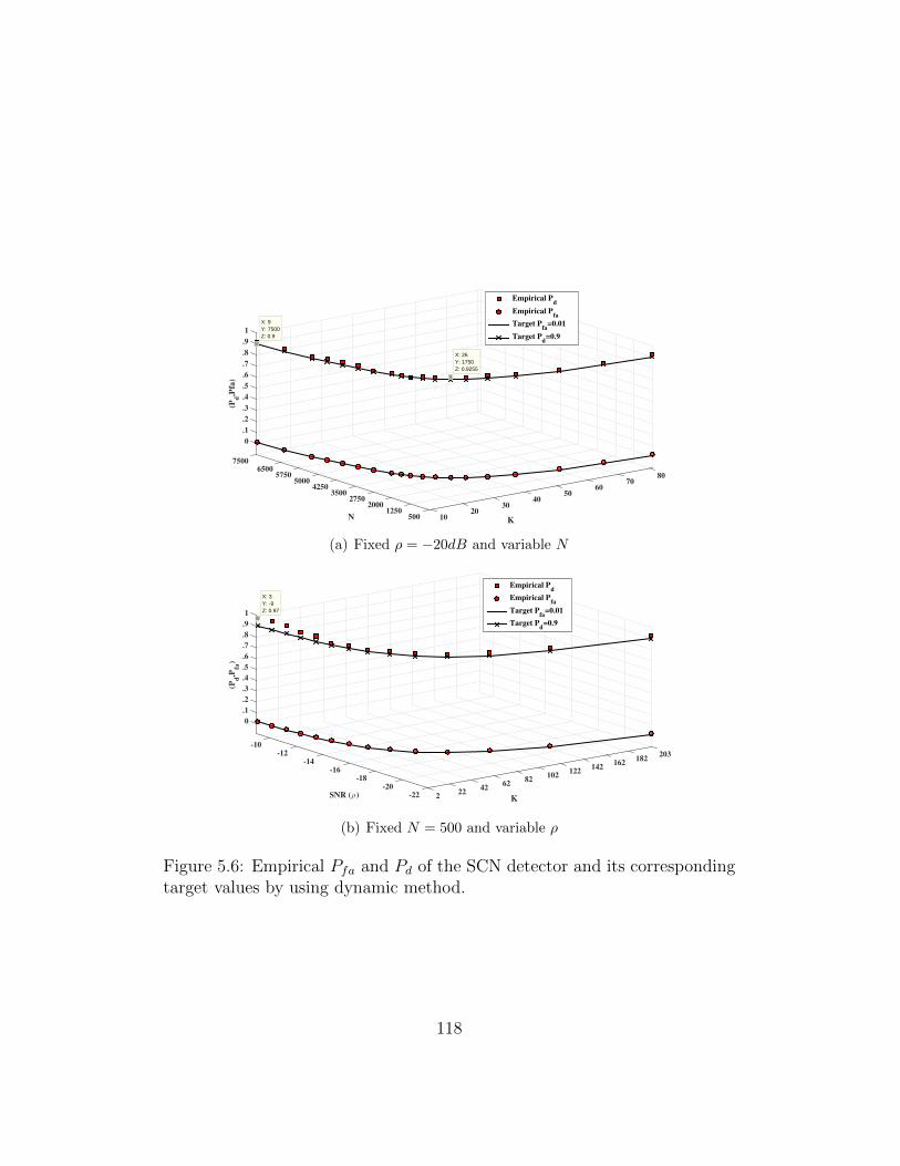
8070
6050
40
K
3020
105001250
20002750
N
35004250
50005750
6500
.1
.2
.6
0
1
.7
.5
.4
.9
.3
.8
7500
(Pd,P
fa)
Empirical Pd
Empirical Pfa
Target Pfa
=0.01
Target Pd=0.9
X: 9Y: 7500Z: 0.9
X: 26Y: 1750Z: 0.9255
(a) Fixed ρ = −20dB and variable N
203182
162142
122102
82
K
6242
222-22
-20-18
SNR (ρ)
-16-14
-12-10
.4
.5
.6
.7
.8
.9
1
0
.1
.3
.2
(Pd,P
fa)
Empirical Pd
Empirical Pfa
Target Pfa
=0.01
Target Pd=0.9
X: 3Y: -9Z: 0.97
(b) Fixed N = 500 and variable ρ
Figure 5.6: Empirical Pfa and Pd of the SCN detector and its correspondingtarget values by using dynamic method.
118
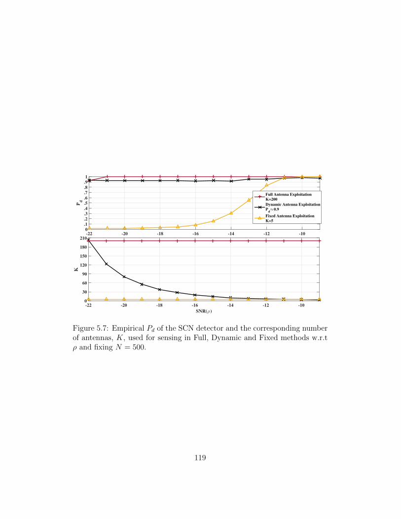
-22 -20 -18 -16 -14 -12 -10
Pd
0
.1
.2
.3
.4
.5
.6
.7
.8
.9
1
Full Antenna Exploitation
K=200
Dynamic Antenna Exploitation
Pd≈0.9
Fixed Antenna Exploitation
K=5
SNR(ρ)
-22 -20 -18 -16 -14 -12 -10
K
0
30
60
90
120
150
180
210
Figure 5.7: Empirical Pd of the SCN detector and the corresponding numberof antennas, K, used for sensing in Full, Dynamic and Fixed methods w.r.tρ and fixing N = 500.
119
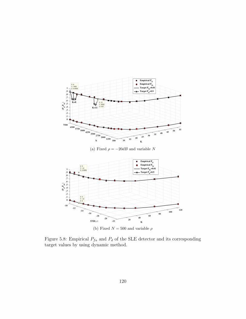
5550
4540
3530
25
K
2015
105001250
20002750
N
35004250
50005750
6500
.8
.7
.5
.9
.3
.2
.1
.6
0
.4
1
7500
(Pd,P
fa)
Empirical Pd
Empirical Pfa
Target Pfa
=0.01
Target Pd=0.9
X: 11Y: 4000Z: 0.87
X: 8Y: 7500Z: 0.9358
K=8
K=11
(a) Fixed ρ = −20dB and variable N
120100
8060
K
4020
-22
-20
-18
SNR(ρ)
-16
-14
-12
.1
0
.2
.3
.4
.5
.6
.7
.8
.9
1
-10
(Pd,P
fa)
Empirical Pd
Empirical Pfa
Target Pfa
=0.01
Target Pd=0.9
X: 5Y: -12Z: 0.9956
X: 5Y: -12Z: 0
(b) Fixed N = 500 and variable ρ
Figure 5.8: Empirical Pfa and Pd of the SLE detector and its correspondingtarget values by using dynamic method.
120
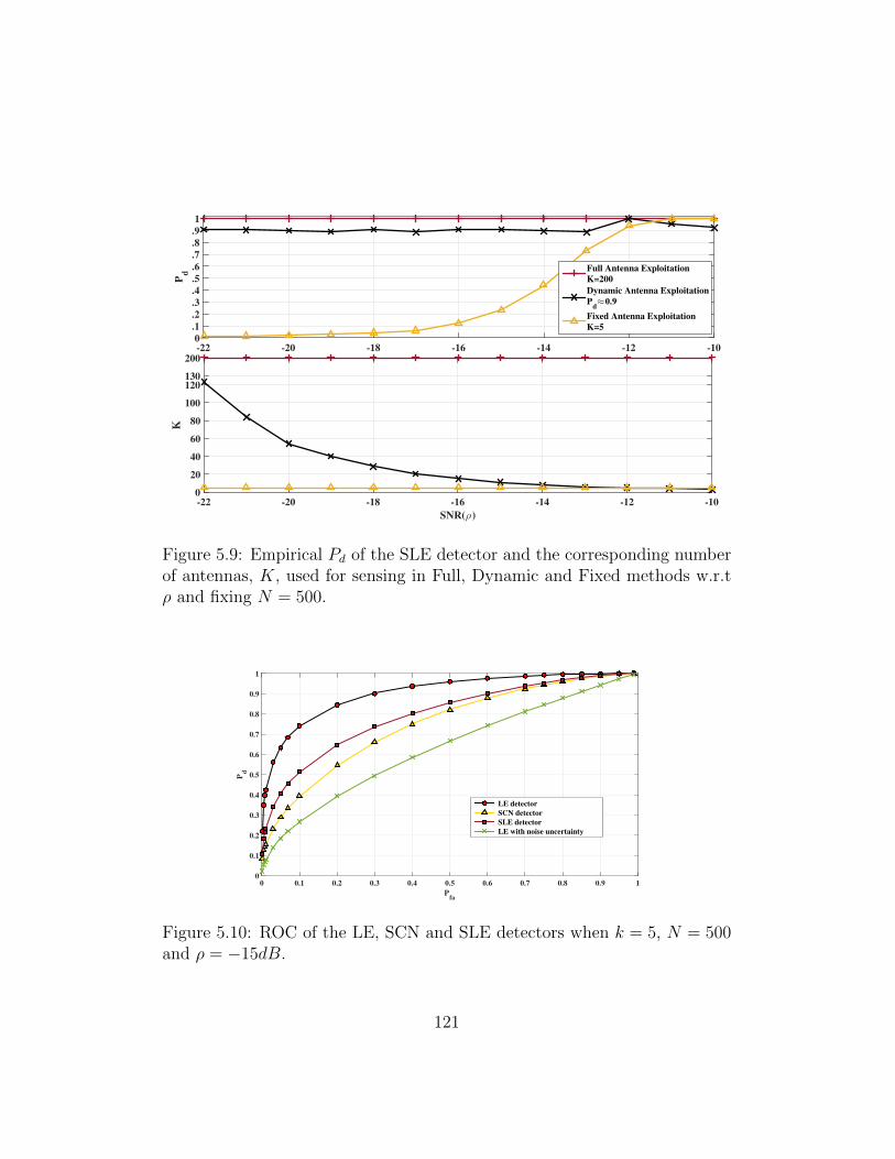
-22 -20 -18 -16 -14 -12 -10
Pd
0
.1
.2
.3
.4
.5
.6
.7
.8
.9
1
Full Antenna Exploitation
K=200
Dynamic Antenna Exploitation
Pd≈0.9
Fixed Antenna Exploitation
K=5
SNR(ρ)
-22 -20 -18 -16 -14 -12 -10
K
0
20
40
60
80
100
120130
200
Figure 5.9: Empirical Pd of the SLE detector and the corresponding numberof antennas, K, used for sensing in Full, Dynamic and Fixed methods w.r.tρ and fixing N = 500.
Pfa
0 0.1 0.2 0.3 0.4 0.5 0.6 0.7 0.8 0.9 1
Pd
0
0.1
0.2
0.3
0.4
0.5
0.6
0.7
0.8
0.9
1
LE detector
SCN detector
SLE detector
LE with noise uncertainty
Figure 5.10: ROC of the LE, SCN and SLE detectors when k = 5, N = 500and ρ = −15dB.
121
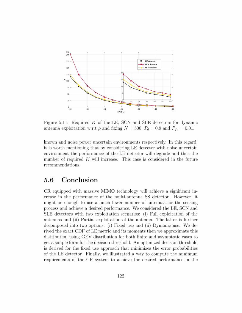
SNR (ρ)
-22 -20 -18 -16 -14 -12 -10
K
0
25
50
75
100
125
150
175
200
210
LE detector
SCN detector
SLE detector
-16 -15 -14 -13 -12 -11 -100
5
10
15
20
Figure 5.11: Required K of the LE, SCN and SLE detectors for dynamicantenna exploitation w.r.t ρ and fixing N = 500, Pd = 0.9 and Pfa = 0.01.
known and noise power uncertain environments respectively. In this regard,it is worth mentioning that by considering LE detector with noise uncertainenvironment the performance of the LE detector will degrade and thus thenumber of required K will increase. This case is considered in the futurerecommendations.
5.6 Conclusion
CR equipped with massive MIMO technology will achieve a significant in-crease in the performance of the multi-antenna SS detector. However, itmight be enough to use a much fewer number of antennas for the sensingprocess and achieve a desired performance. We considered the LE, SCN andSLE detectors with two exploitation scenarios: (i) Full exploitation of theantennas and (ii) Partial exploitation of the antenna. The latter is furtherdecomposed into two options: (i) Fixed use and (ii) Dynamic use. We de-rived the exact CDF of LE metric and its moments then we approximate thisdistribution using GEV distribution for both finite and asymptotic cases toget a simple form for the decision threshold. An optimized decision thresholdis derived for the fixed use approach that minimizes the error probabilitiesof the LE detector. Finally, we illustrated a way to compute the minimumrequirements of the CR system to achieve the desired performance in the
122
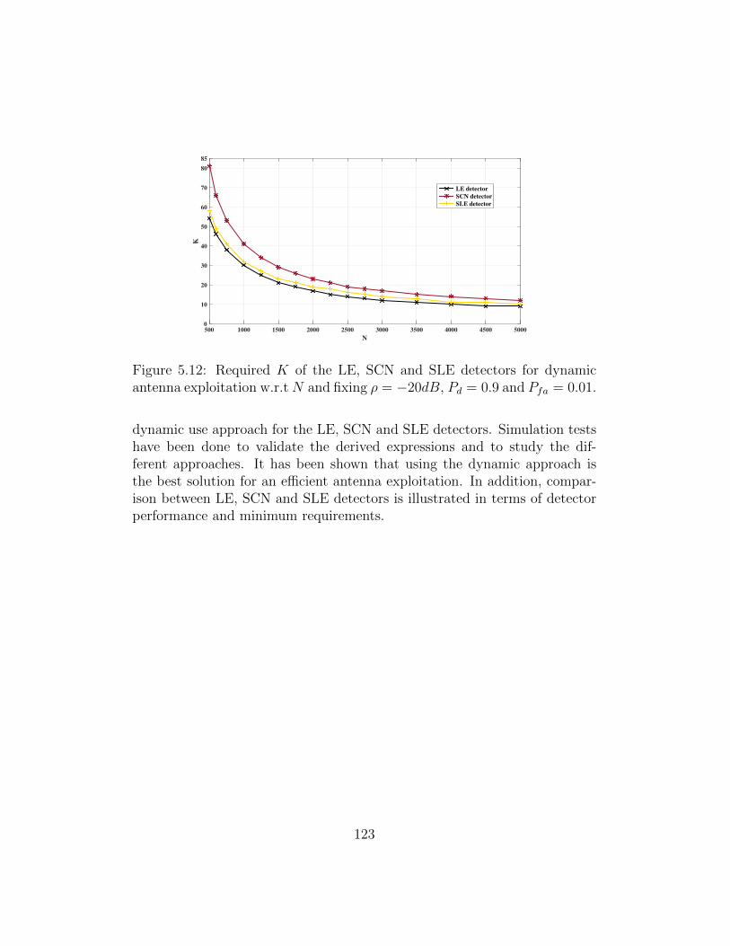
N
500 1000 1500 2000 2500 3000 3500 4000 4500 5000
K
0
10
20
30
40
50
60
70
80
85
LE detector
SCN detector
SLE detector
Figure 5.12: Required K of the LE, SCN and SLE detectors for dynamicantenna exploitation w.r.tN and fixing ρ = −20dB, Pd = 0.9 and Pfa = 0.01.
dynamic use approach for the LE, SCN and SLE detectors. Simulation testshave been done to validate the derived expressions and to study the dif-ferent approaches. It has been shown that using the dynamic approach isthe best solution for an efficient antenna exploitation. In addition, compar-ison between LE, SCN and SLE detectors is illustrated in terms of detectorperformance and minimum requirements.
123
Chapter 6
Conclusions and Future
Recommendations
In this thesis, we have considered the EBD in a multiple-antenna CR systems.EBD is usually a blind detector that overcomes noise uncertainty problemsand is efficient in low SNR environments. Moreover, the use of multi-antennatechnology in CR further extends the detection of spectrum holes from theconventional frequency-time-space dimensions to a wider space that includesthe angle-of-arrival dimension. However, the main disadvantage of the EBDis the complexity of its performance probabilities and the threshold whichcannot be evaluated on the fly. Moreover, the concept of massive MIMO inSS and CRs still needs to be explored. There are various contributions in theareas presented in this thesis and detailed in [J1-J5, C1-C3] and summarizedas follows:
In Chapter 3, we considered the SCN detector and discussed the com-plexity of its decision metric distribution expressions, i.e. PDF and CDF.This would result in complicated forms for the probability and the deci-sion threshold which could not be computed online. In this regard, we havestarted by deriving the analytical expression of the joint distribution of theordered eigenvalues of the central semi-correlated Wishart matrices when thesome of the eigenvalues of the correlation matrix are equal. We studied thenon-central/central approximation empirically and showed that it has per-fect accuracy for low SNR values and could be considered as a good fit forPd for sufficiently large values of N when the SNR is high. The finite caseof the SCN detector is considered next. We derived the exact distribution of
124
the SCN of the central uncorrelated, central semi-correlated and non-centraluncorrelated Wishart matrices. In addition, the p-th moment of the SCNis considered as we derived the exact form for the pre-mentioned Wishartmatrices. To overcome the computational complexity of the exact SCN dis-tribution, we proposed to approximate it using the GEV distribution basedon moment matching criteria. Accordingly, an approximation for the perfor-mance probabilities of the SCN detector and its decision threshold are giventhrough simple expressions. Moreover, and using the non-central/centralapproximation we have proposed a 2-step approximation for the detectionprobability of the SCN detector which provides similar accuracy with sim-pler moment complexity. Finally, in the asymptotic case, We derived theasymptotic mean, the asymptotic variance and the asymptotic skewness ofthe SCN using those of the extreme eigenvalues of the sample covariancematrix by means of bi-variate Taylor expansion. GEV approximation forthe distribution of the SCN under H0 and H1 hypotheses were proposed.Consequently, simple forms for the false-alarm probability, detection proba-bility and the decision threshold are derived for real-time computations suchthat a CR system with large number of antennas can dynamically adapt itsthreshold according to pre-defined error constraints and channel conditions.
In Chapter 4, we considered the SLE detector which is an optimal detectorfor detecting a single-PU in uncertain noise environments. We discussed thecomplexity of its decision metric distribution expressions in literature thatare based on TW2 distribution or derived using Mellin transform. We provedthat the SLE could be modeled using standard Gaussian function under someconstraints. We showed that the trace is a Gaussian RV using the CLT. Wederived the CDF and the PDF of the SLE based on the distributions of thelargest eigenvalue and the trace. The false alarm probability, the detectionprobability and the decision threshold were also considered as we derived newsimple and accurate forms. These forms are simple functions of the meansand variances of the largest eigenvalue and the trace as well as the correlationcoefficient between them. The correlation between the largest eigenvalue andthe trace is studied and simple expressions are provided.
In Chapter 5, we considered a CR equipped with massive MIMO tech-nology. We discussed different scenarios for SS using these large numberof antennas. In the first scenario, we considered that the CR will use allthese antennas for SS and thus we approximate the LE using the GEV ap-proximation under H0 hypothesis while keeping the Gaussian approximationunder H1 hypothesis. Accordingly, the threshold could be set. In the second
125
scenario, we considered two approaches: (i) fixed resource and (ii) dynamicresources. For this scenario, an optimal threshold for the LE detector wasderived and the minimum required resources are discussed for the LE detec-tor if noise power is perfectly known and for SCN and SLE detectors whennoise uncertainty exists. we showed that the dynamic approach is the bestsolution for an efficient antenna exploitation while maintaining on a targetperformance. We showed the importance of this scenario from different as-pects.
Finally, we present open research problems and future recommendationsrelated to the topics discussed in this thesis:
1. Noise power uncertainty: In practical scenarios, the cognitive receiveris affected by several factors such as interference, noise uncertainty,channel uncertainty etc.. It is still an open challenge to model the LEdetector in noise uncertain environments.
2. Noise correlation: In practice, the noise is never white and noise correla-tion is indeed a big challenge for EBD. Modelling the noise correlationand studying their effect on different decision metrics of the EBD ishighly recommended for future work.
3. Hardware implementation and real scenario comparison: As mentioned,several factors will affect the detection performance for any detectorin practical scenarios. Hence, it would be interesting to implementthe mentioned detectors using USRPs and study their performancesin real scenario. Moreover, performance comparison of these detectorsand others, like ED and CFD, in real environments is very importantfor future use of any of the mentioned detectors.
4. Massive MIMO:
– Antenna Selection: as discussed in Ch. 5, dynamic antenna ex-ploitation is very important for an efficient exploitation of the hugenumber of antenna that a CR is equipped with. Thus, the antennaselection criteria is worth considered in future work. Moreover, theexploitation of beam-forming for detecting the angle-of-arrival ofthe signal must be considered in the antenna clustering or selectioncriteria.
126
5. Hybrid Cooperative Detectors: As discussed in Ch. 2, cooperative spec-trum sensing has several benefits such as avoiding HNP and increasingthe sensing performance. On the other hand, different devices may havedifferent capabilities and may face different environmental conditions.Here, according to device capability, to the amount of knowledge andenvironmental conditions, the SU may use different detector for spec-trum sensing. For example, if the SU device is equipped with singleantenna then it may use ED whereas a multi-antenna device with per-fect noise power knowledge may use LE detector and so on. Then, thecooperation between different SUs using different detectors is worthconsidered and modeled.
127
Appendix A
Proofs
A.1 Proof of Theorem 3.1
Before we start the proof, it is required to give the following Lemma present-ing the nth derivative of any function of the form e−
ax with respect to the
variable x.
Lemma A.1. let us define the function f(x) = e−ax , then the nth derivative
of f(x) is given by:
f (n)(x) =a
x2n· e−
ax ·[ n∑k=1
(−1)k+nL(n, k)xn−kak−1
](A.1)
where the Lah number defined by L(n, k) =(nk
)(n−1k−1
)(n− k)!.
Proof. It should be noted that, for any value of n, the nth derivative of e−ax
will result into the function e−ax multiplied by sum of (a/x) with different
powers for a and x. Regardless of the sign, it is found that the number mul-tiplied by each component of this sum is exactly equals to the Lah number.
Following the pattern seen by calculating the derivative of f(x) for smallvalues of n, and matching the numbers at each derivative level, ”n”, with theLah number L(n, k), it can be proved, by recurrence, that the nth derivativeof the function f(x) of the form e−
ax is given by (A.1).
Now, we proceed in proving theorem A.2. If we have L equal eigenvalues(σp = · · · = σq), we must generalize the result of central semi-correlated
128
Wishart with distinct correlation eigenvalues for arbitrary number of coinci-dent eigenvalues by taking the limit of joint distribution given by [157, Eq.6] as follows:
limσp,q→σp
f(λ)= |Φ(λ)|K∏i=1
ξ(λi) limσp,q→σp
(C×|E(λ,σ)|) (A.2)
= |Φ(λ)|K∏i=1
ξ(λi) limσp,q→σp
∏K
i<j σiσjK∏i=1
σNi (N − i)!· |E(λ,σ)|K∏i<j
σj − σi
with σp,q = [σp, · · · , σq], and C the normalization constant, Φ(λ) is a Van-
dermonde matrix of entries λi−1j , E(λ,σ) is matrix of entries e
−λj/σi , and
ξ(λi) = λN−Ki [157, Table I]. To evaluate the limit in (A.2) we apply lemma2 from [216] to obtain:
limσp,q→σp
|E(λ,σ)|K∏i<j
σj − σi=
∣∣∣∣∣∣∣∣∣∣∣∣∣∣∣∣∣∣∣∣
e(λ1, σ1) · · · · · · e(λK , σ1)...
. . . . . ....
e(λ1, σp−1) · · · · · · e(λK , σp−1)e(L−1)(λ1, σp) · · · · · · e(L−1)(λK , σp)
.... . . . . .
...e(0)(λ1, σp) · · · · · · e(0)(λK , σp)e(λ1, σq+1) · · · · · · e(λK , σq+1)
.... . . . . .
...e(λ1, σK) · · · · · · e(λK , σK)
∣∣∣∣∣∣∣∣∣∣∣∣∣∣∣∣∣∣∣∣K∏i<jσi 6=σj
(σj − σi) · ΓL(L)
(A.3)
with e(λi, σj) = e− λiσj , the required derivatives are evaluated using (A.1) and
Γs(l) =∏s
i=1(l − i)!. Then, the result is obtained by substituting (A.1) and(A.3) into (A.2) and simplifying.
In the case we have several coincidence (eg. σp,q = σp, σt,s = σs, etc.),the same analysis could be applied and the limit must be taken over allcoincidence cases.
129

A.2 Proof of Equations 3.16-3.17, 3.22-3.23,
3.29-3.30.
Consider the equations (3.14), (3.19) and (3.26) and apply Laplace expansionfollowed by Leibniz formula of the determinant [217] we get:
F (x) = K.K∑
n,m=1
(−1)n+m∑δ∈P1
sgn(δ)
∫ ∞0
Υ.n,m(λK)K−1∏i=1
∫ xλK
λK
Υ.rδi,n,ri,m(u)du dλK
(A.4)where . refers to one of these cases (cu: central uncorrelated, nu: non-central uncorrelated, or cc: central semi-correlated).
Knowing that γ(n, λ) = (n − 1)!(
1− e−λ∑n−1
l=0λl
l!
)and 0F1(n, λ) =∑∞
l=0λl
(n)ll!, then (3.16), (3.22) and (3.29) are derived as follows:
• substitute (3.15), (3.20) or (3.27) in (A.4) for (3.16), (3.22) and (3.29)respectively.
• algebraic manipulation and integrate.
Equations (3.17), (3.23) and (3.30) are, respectively, the derivatives of(3.16), (3.22) and (3.29).
A.3 Proof of Theorems 3.2 and 3.3
Starting by particularizing the joint distribution of the ordered eigenvaluesof the central semi-correlated Wishart matrices when the correlation matrixhas K − 1 equal eigenvalues, then we have the following Lemma:
Lemma A.2. Let W ∼ CWK(N,Σ) be a central semi-correlated complexWishart matrix with correlation matrix Σ of eigenvalues σ1 > σ2 = · · · = σK.Then, the joint distribution of the ordered eigenvalues of W is given by:
f(λ) = Kcc|V (λ)||E(λ,σ)|K∏l=1
λN−Kl , (A.5)
with (i, j)-th entries of E(λ,σ) and Kcc are given respectively by:
ei(λj) =
e−λjσ1 i = 1
(−λj)K−ie−λjσ2 1 < i ≤ K
(A.6)
130

Kcc =σK−N−1
1 σ(N−1)(1−K)2
ΓK(N)ΓK−1(K − 1)(σ2 − σ1)K−1(A.7)
Now, Using joint distribution in (3.4) and (A.5), then the result in (3.19)and (3.26) follows the analytical derivation of (3.14) while considering thedifferent cases of fi(λj) and ei(λj). Finally, substitute the hypergeometricfunction for the non-central case and integrate using [179, Eq.(3.351.1)].
A.4 Proof of Theorems 3.4, 3.5 and 3.6.
The pth moment of the SCN is given by:
M(p) =
∫ ∞0
∫ ∞λK
· · ·∫ ∞λ2
(λ1
λK)p · f(λ) dλ1 · · · dλK (A.8)
then the result is derived as follows:
• substitute the joint distribution of the ordered eigenvalues for the cen-tral uncorrelated, non-central uncorrelated, and central semi-correlatedWishart cases.
• apply Laplace expansion.
• apply Leibniz formula
• algebraic manipulation to transform the product into sum then collectcommon terms
• integrate using [179, Eq.(3.351.2)] and [179, Eq.(3.351.3)] and watchthe recurrence.
A.5 Proof of Theorems 5.2 and 5.3.
Using integration by parts, the p-th moment of the LE could be written asfollows:
MLEp =
∫ +∞
0
xpd(FLE(x))
= xpFLE(x)
∣∣∣∣+∞0
−∫ +∞
0
pxp−1FLE(x)dx, (A.9)
131
now, using the alternative sum of determinant (Leibniz formula) [217] andthe definition of lower incomplete gamma function [179, Eq. 8.352.1], thenFLE(x) of central uncorrelated and central semi-correlated Wishart matrices,after some algebraic manipulation, could be written, respectively, as follows:
F cuλ1
(x) =Kcu∑δ∈P0
sgn(δ)K∏i=1
(δ(i) + i+N −K − 2)!
×∑s∈S0
(−1)|s|e−|s|xxΣls
Πls!(A.10)
F ccλ1
(x) =K′cc∑δ∈P0
sgn(δ)K∏i=1
(N + δ(i)− bi,K − 1)!
σbi,K−δ(i)−Ni
×∑s∈S0
(−1)|s|e−Σ 1σsxxΣs
Πs! · Πσss(A.11)
Finally, equations (5.6) and (5.7) results after substituting (A.10) and(A.11), respectively, in (A.9) and integrate using [179, Eq. 3.351.3].
132
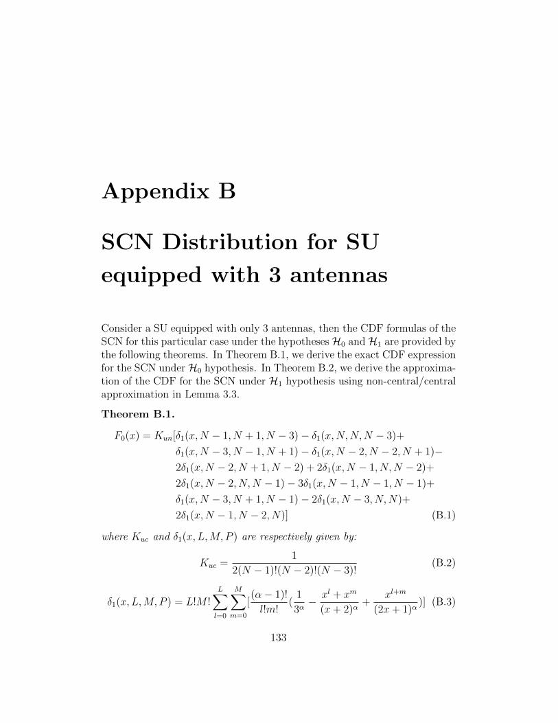
Appendix B
SCN Distribution for SU
equipped with 3 antennas
Consider a SU equipped with only 3 antennas, then the CDF formulas of theSCN for this particular case under the hypothesesH0 andH1 are provided bythe following theorems. In Theorem B.1, we derive the exact CDF expressionfor the SCN under H0 hypothesis. In Theorem B.2, we derive the approxima-tion of the CDF for the SCN under H1 hypothesis using non-central/centralapproximation in Lemma 3.3.
Theorem B.1.
F0(x) = Kun[δ1(x,N − 1, N + 1, N − 3)− δ1(x,N,N,N − 3)+
δ1(x,N − 3, N − 1, N + 1)− δ1(x,N − 2, N − 2, N + 1)−2δ1(x,N − 2, N + 1, N − 2) + 2δ1(x,N − 1, N,N − 2)+
2δ1(x,N − 2, N,N − 1)− 3δ1(x,N − 1, N − 1, N − 1)+
δ1(x,N − 3, N + 1, N − 1)− 2δ1(x,N − 3, N,N)+
2δ1(x,N − 1, N − 2, N)] (B.1)
where Kuc and δ1(x, L,M, P ) are respectively given by:
Kuc =1
2(N − 1)!(N − 2)!(N − 3)!(B.2)
δ1(x, L,M, P ) = L!M !L∑l=0
M∑m=0
[(α− 1)!
l!m!(
1
3α− xl + xm
(x+ 2)α+
xl+m
(2x+ 1)α)] (B.3)
133
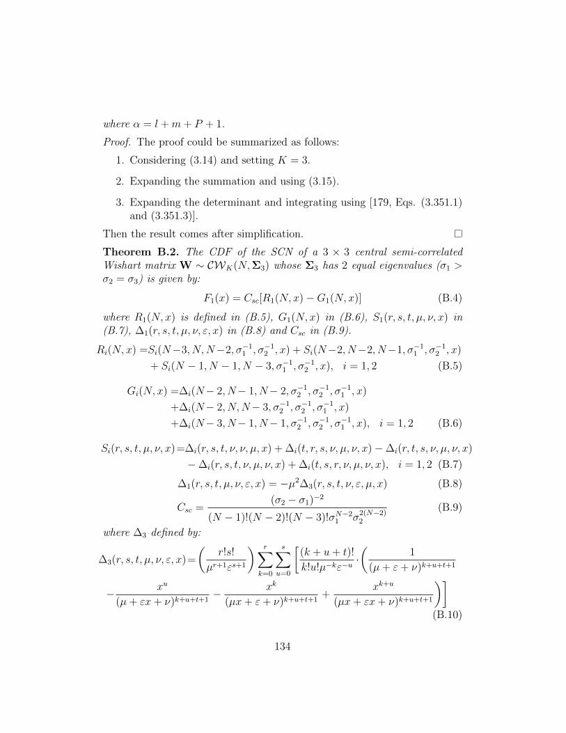
where α = l +m+ P + 1.
Proof. The proof could be summarized as follows:
1. Considering (3.14) and setting K = 3.
2. Expanding the summation and using (3.15).
3. Expanding the determinant and integrating using [179, Eqs. (3.351.1)and (3.351.3)].
Then the result comes after simplification.
Theorem B.2. The CDF of the SCN of a 3 × 3 central semi-correlatedWishart matrix W ∼ CWK(N,Σ3) whose Σ3 has 2 equal eigenvalues (σ1 >σ2 = σ3) is given by:
F1(x) = Csc[R1(N, x)−G1(N, x)] (B.4)
where R1(N, x) is defined in (B.5), G1(N, x) in (B.6), S1(r, s, t, µ, ν, x) in(B.7), ∆1(r, s, t, µ, ν, ε, x) in (B.8) and Csc in (B.9).
Ri(N, x) =Si(N−3, N,N−2, σ−11 , σ−1
2 , x) + Si(N−2, N−2, N−1, σ−11 , σ−1
2 , x)
+ Si(N − 1, N − 1, N − 3, σ−11 , σ−1
2 , x), i = 1, 2 (B.5)
Gi(N, x) =∆i(N− 2, N− 1, N− 2, σ−12 , σ−1
2 , σ−11 , x)
+∆i(N− 2, N,N− 3, σ−12 , σ−1
2 , σ−11 , x)
+∆i(N− 3, N− 1, N− 1, σ−12 , σ−1
2 , σ−11 , x), i = 1, 2 (B.6)
Si(r, s, t, µ, ν, x)=∆i(r, s, t, ν, ν, µ, x) + ∆i(t, r, s, ν, µ, ν, x)−∆i(r, t, s, ν, µ, ν, x)
−∆i(r, s, t, ν, µ, ν, x) + ∆i(t, s, r, ν, µ, ν, x), i = 1, 2 (B.7)
∆1(r, s, t, µ, ν, ε, x) = −µ2∆3(r, s, t, ν, ε, µ, x) (B.8)
Csc =(σ2 − σ1)−2
(N − 1)!(N − 2)!(N − 3)!σN−21 σ
2(N−2)2
(B.9)
where ∆3 defined by:
∆3(r, s, t, µ, ν, ε, x)=
(r!s!
µr+1εs+1
) r∑k=0
s∑u=0
[(k + u+ t)!
k!u!µ−kε−u·(
1
(µ+ ε+ ν)k+u+t+1
− xu
(µ+ εx+ ν)k+u+t+1− xk
(µx+ ε+ ν)k+u+t+1+
xk+u
(µx+ εx+ ν)k+u+t+1
)](B.10)
134

Proof. The proof could be summarized as follows:
1. Considering (3.26) and setting K = 3.
2. Substituting the parameters from Lemma A.2.
3. Expanding the summation and using (3.28).
4. Expanding the determinant and integrating using [179, Eqs. (3.351.1)and (3.351.3)].
Then the result comes after simplification.
It is worth mentionning that the PDF expressions are the derivative ofthe CDF expressions w.r.t x.
135

Appendix C
Generalized Extreme Value
Distribution
Generalized Extreme Value (GEV) is a flexible 3-parameter distribution usedto model the extreme events of a sequence of i.i.d random variables. The GEVparameters are the location parameter (µ εR), the scale parameter (σ > 0),and the shape parameter (ξ εR). Various values of the shape parameter yieldto a type of the extreme value distributions [218].
Let X be a GEV distributed random variable, then the CDF and thePDF of X are given by [218]:
F (x;µ, σ, ξ) = e−t(x), (C.1)
f(x;µ, σ, ξ) =1
σt(x)ξ+1e−t(x), (C.2)
with t(x) given by (C.3).
t(x) =
e−
x−µσ ξ = 0
(1 + (x−µσ
)ξ)−1/ξ ξ 6= 0
. (C.3)
The mean, variance and skewness of the X are given in Table C.1 wheregk = Γ(1− kξ), γ is Euler’s constant, and ζ(.) is the Riemann zeta function,with Γ(.) is the gamma function [219].
Finding the inverse function of the skewness in Table C.1 is not straight-forward, thus, applying non-linear least squares change this inversion into
136
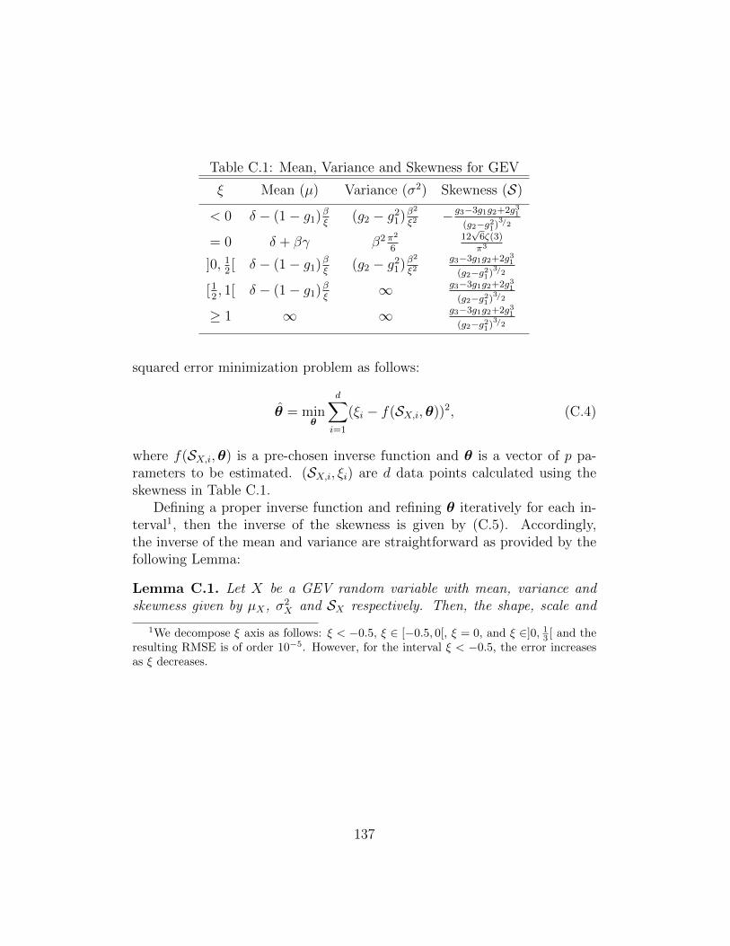
Table C.1: Mean, Variance and Skewness for GEV
ξ Mean (µ) Variance (σ2) Skewness (S)
< 0 δ − (1− g1)βξ
(g2 − g21)β
2
ξ2 −g3−3g1g2+2g31
(g2−g21)
3/2
= 0 δ + βγ β2 π2
612√
6ζ(3)π3
]0, 12[ δ − (1− g1)β
ξ(g2 − g2
1)β2
ξ2
g3−3g1g2+2g31
(g2−g21)
3/2
[12, 1[ δ − (1− g1)β
ξ∞ g3−3g1g2+2g3
1
(g2−g21)
3/2
≥ 1 ∞ ∞ g3−3g1g2+2g31
(g2−g21)
3/2
squared error minimization problem as follows:
θ = minθ
d∑i=1
(ξi − f(SX,i,θ))2, (C.4)
where f(SX,i,θ) is a pre-chosen inverse function and θ is a vector of p pa-rameters to be estimated. (SX,i, ξi) are d data points calculated using theskewness in Table C.1.
Defining a proper inverse function and refining θ iteratively for each in-terval1, then the inverse of the skewness is given by (C.5). Accordingly,the inverse of the mean and variance are straightforward as provided by thefollowing Lemma:
Lemma C.1. Let X be a GEV random variable with mean, variance andskewness given by µX , σ2
X and SX respectively. Then, the shape, scale and
1We decompose ξ axis as follows: ξ < −0.5, ξ ∈ [−0.5, 0[, ξ = 0, and ξ ∈]0, 13 [ and theresulting RMSE is of order 10−5. However, for the interval ξ < −0.5, the error increasesas ξ decreases.
137

location of X are given, respectively, by:
ξ =
a1 ln(b1S2
X + c1SX + d1) SX < −0.63
a2S2X + b2SX + c2 −0.63 ≤ SX < 1.14
0 SX = 1.14a3S2
X+b3SX+c3S2X+d3SX+e3
SX > 1.14
(C.5)
β =
√
σ2Xξ
2
g2−g21SX 6= 1.14√
6σ2X
πSX = 1.14
(C.6)
δ =
µX − (g1−1)σ
ξSX 6= 1.14
µX − σγ SX = 1.14(C.7)
where the constants in (C.5) are given in Table C.2.
Table C.2: Constants of Eq. (C.5), Lemma C.1
i ai bi ci di ei
1 −0.43544 2.3227 −0.97563 1.3781 −2 −0.06393 0.3173 −0.2771 − −3 0.333 −0.09862 −0.3195 0.9553 1.599
138
Bibliography
[1] K. Patil, R. Prasad, and K. Skouby, “A survey of worldwide spec-trum occupancy measurement campaigns for cognitive radio,” in De-vices and Communications (ICDeCom), 2011 International Conferenceon, pp. 1–5, Feb 2011.
[2] D. Datla, A. M. Wyglinski, and G. J. Minden, “A spectrum surveyingframework for dynamic spectrum access networks,” IEEE Transactionson Vehicular Technology, vol. 58, pp. 4158–4168, Oct 2009.
[3] K. Patil, K. E. Skouby, and R. Prasad, “Spectrum measurement andanalysis of tv band support of cognitive radio operation in india,” inWireless Communications, Vehicular Technology, Information Theoryand Aerospace Electronic Systems (VITAE), 2013 3rd InternationalConference on, pp. 1–5, June 2013.
[4] D. Das and S. Das, “A survey on spectrum occupancy measurementfor cognitive radio,” Wireless Personal Communications, vol. 85, no. 4,pp. 2581–2598, 2015.
[5] FCC, “Et docket no 02-135: spectrum policy task force report,” Nov.2002.
[6] FCC, “Et docket no. 03-108: Facilitating opportunities for flexible,efficient, and reliable spectrum use employing cognitive radio technolo-gies,” March 2005.
[7] L. Berlemann and S. Mangold, Cognitive Radio and Dynamic SpectrumAccess. WILEY, 1st ed., 2009.
[8] Q. Zhao and B. M. Sadler, “A survey of dynamic spectrum access,”IEEE Signal Processing Magazine, vol. 24, pp. 79–89, May 2007.
139
[9] J. Mitola and G. Q. Maguire, “Cognitive radio: making software radiosmore personal,” IEEE Personal Communications, vol. 6, pp. 13–18,Aug 1999.
[10] B. Wang and K. J. R. Liu, “Advances in cognitive radio networks: Asurvey,” IEEE Journal of Selected Topics in Signal Processing, vol. 5,pp. 5–23, Feb 2011.
[11] C. R. Stevenson, G. Chouinard, Z. Lei, W. Hu, S. J. Shellhammer, andW. Caldwell, “Ieee 802.22: The first cognitive radio wireless regionalarea network standard,” IEEE Communications Magazine, vol. 47,pp. 130–138, January 2009.
[12] “Standard for cognitive wireless regional area networks (ran) for oper-ation in tv bands,” July 2011.
[13] ETSI-RRS, “Mobile broadband services in the 23002400 mhz frequencyband under licensed shared access regime,” tr 103.113, ETSI, 2013.
[14] ETSI-RRS, “System reference document; mobile broadband services inthe 2300 mhz 2400 mhz frequency band under licensed shared accessregime,” ts 103.154, ETSI, 2014.
[15] ETSI-RRS, “System architecture and high level procedures for opera-tion of licensed shared access (lsa) in the 2300 mhz-2400 mhz band,”ts 103.235, ETSI, 2015.
[16] FCC, “Third memorandum opinion and order,” FCC 12-36, April 2012.
[17] OFCOM, “Regulatory requirements for white space device in the uhftv band,” tech. rep., OFCOM, July 2012.
[18] C. S. Sum, G. P. Villardi, M. A. Rahman, T. Baykas, H. N. Tran,Z. Lan, C. Sun, Y. Alemseged, J. Wang, C. Song, C. W. Pyo, S. Filin,and H. Harada, “Cognitive communication in tv white spaces: Anoverview of regulations, standards, and technology [accepted from opencall],” IEEE Communications Magazine, vol. 51, pp. 138–145, July2013.
140

[19] M. Nekovee, “Cognitive radio access to tv white spaces: Spectrumopportunities, commercial applications and remaining technology chal-lenges,” in New Frontiers in Dynamic Spectrum, 2010 IEEE Sympo-sium on, pp. 1–10, April 2010.
[20] T. Yucek and H. Arslan, “A survey of spectrum sensing algorithms forcognitive radio applications,” IEEE Communications Surveys Tutori-als,, vol. 11, no. 1, pp. 116–130, 2009.
[21] D. Cabric, A. Tkachenko, and R. W. Brodersen, “Spectrum sensingmeasurements of pilot, energy, and collaborative detection,” in MIL-COM 2006 - 2006 IEEE Military Communications conference, pp. 1–7,Oct 2006.
[22] S. P. Herath, N. Rajatheva, and C. Tellambura, “Energy detection ofunknown signals in fading and diversity reception,” IEEE Transactionson Communications, vol. 59, pp. 2443–2453, September 2011.
[23] C. H. Lim, “Adaptive energy detection for spectrum sensing in un-known white gaussian noise,” IET Communications, vol. 6, pp. 1884–1889, Sept 2012.
[24] M. Gautier, V. Berg, and D. Noguet, “Wideband frequency domaindetection using Teager-Kaiser energy operator,” in IEEE 5th Interna-tional Conference on Cognitive Radio Oriented Wireless Networks andCommunications (Crowncom’12), (Stockholm, Sweden), June 2012.
[25] J. Palicot and C. Roland, “A new concept for wireless reconfigurablereceivers,” IEEE Communications Magazine, vol. 41, pp. 124–132, July2003.
[26] R. Chen and J. M. Park, “Ensuring trustworthy spectrum sensing incognitive radio networks,” in Networking Technologies for Software De-fined Radio Networks, 2006. SDR ’06.1st IEEE Workshop on, pp. 110–119, Sept 2006.
[27] Z. Khalaf, A. Nafkha, and J. Palicot, “Blind cyclostationary featuredetector based on sparsity hypotheses for cognitive radio equipment,”in 2011 IEEE 54th International Midwest Symposium on Circuits andSystems (MWSCAS), pp. 1–4, Aug 2011.
141
[28] Z. Khalaf, J. Palicot, A. Nafkha, and H. Zhang, “Blind free band de-tector based on the sparsity of the cyclic autocorrelation function,” inEUSIPCO, (Morocco), Sep. 2013.
[29] M. Kosunen, V. Turunen, K. Kokkinen, and J. Ryynnen, “Survey andanalysis of cyclostationary signal detector implementations on fpga,”IEEE Journal on Emerging and Selected Topics in Circuits and Sys-tems, vol. 3, pp. 541–551, Dec 2013.
[30] J. Riba, J. Font-Segura, J. Villares, and G. Vzquez, “Frequency-domainglr detection of a second-order cyclostationary signal over fading chan-nels,” IEEE Transactions on Signal Processing, vol. 62, pp. 1899–1912,April 2014.
[31] P. Urriza, E. Rebeiz, and D. Cabric, “Multiple antenna cyclostation-ary spectrum sensing based on the cyclic correlation significance test,”IEEE Journal on Selected Areas in Communications, vol. 31, pp. 2185–2195, November 2013.
[32] R. Tandra and A. Sahai, “Fundamental limits on detection in low snrunder noise uncertainty,” in in WirelessCom 2005, Maui, HI, 2005.
[33] C. Jiang, Y. Li, W. Bai, Y. Yang, and J. Hu, “Statistical matchedfilter based robust spectrum sensing in noise uncertainty environment,”in Communication Technology (ICCT), 2012 IEEE 14th InternationalConference on, pp. 1209–1213, Nov 2012.
[34] D. Bhargavi and C. R. Murthy, “Performance comparison of energy,matched-filter and cyclostationarity-based spectrum sensing,” in Sig-nal Processing Advances in Wireless Communications (SPAWC), 2010IEEE Eleventh International Workshop on, pp. 1–5, June 2010.
[35] S. Kapoor, S. Rao, and G. Singh, “Opportunistic spectrum sensing byemploying matched filter in cognitive radio network,” in Communica-tion Systems and Network Technologies (CSNT), 2011 InternationalConference on, pp. 580–583, June 2011.
[36] L. Cardoso, M. Debbah, P. Bianchi, and J. Najim, “Cooperative spec-trum sensing using random matrix theory,” in in Proc. IEEE Int. Symp.Wireless Pervasive Comput. (ISWPC), (Greece), pp. 334–338, May2008.
142
[37] F. Penna, R. Garello, and M. Spirito, “Cooperative spectrum sensingbased on the limiting eigenvalue ratio distribution in wishart matrices,”IEEE Commun. Letters,, vol. 13, pp. 507–509, July 2009.
[38] Y. Zeng and Y.-C. Liang, “Eigenvalue-based spectrum sensing algo-rithms for cognitive radio,” IEEE Trans. Commun., vol. 57, pp. 1784–1793, June 2009.
[39] R. Zhang, T. J. Lim, Y.-C. Liang, and Y. Zeng, “Multi-antenna basedspectrum sensing for cognitive radios: A glrt approach,” IEEE Trans.Comm., vol. 58, pp. 84–88, January 2010.
[40] P. Bianchi, M. Debbah, M. Maida, and J. Najim, “Performance of sta-tistical tests for single-source detection using random matrix theory,”IEEE Trans. Inform. Theory,, vol. 57, pp. 2400–2419, April 2011.
[41] P. Wang, J. Fang, N. Han, and H. Li, “Multiantenna-assisted spectrumsensing for cognitive radio,” Vehicular Technology, IEEE Transactionson, vol. 59, pp. 1791–1800, May 2010.
[42] B. Nadler, F. Penna, and R. Garello, “Performance of eigenvalue-basedsignal detectors with known and unknown noise level,” in Communi-cations (ICC), 2011 IEEE International Conference on, pp. 1–5, June2011.
[43] L. Wei and O. Tirkkonen, “Spectrum sensing in the presence of mul-tiple primary users,” IEEE Transactions on Communications, vol. 60,pp. 1268–1277, May 2012.
[44] W. Zhang, G. Abreu, M. Inamori, and Y. Sanada, “Spectrum sensingalgorithms via finite random matrices,” IEEE Trans. Commun., vol. 60,pp. 164–175, January 2012.
[45] A. M. Tulino and S. Verd?, Random Matrix Theory and Wireless Com-munications. now Publishers Inc., 2004.
[46] R. Couillet and M. Debbah, Random Matrix Theory for Wireless Com-munications. Cambridge University Press, Sep. 2011.
[47] H. Venkataraman and G.-M. Muntean, eds., COGNITIVE RADIOAND ITS APPLICATION FOR NEXT GENERATION CELLULARAND WIRELESS NETWORKS. Springer, 2012.
143
[48] J. Neel, Analysis and Design of Cognitive Radio Networks and Dis-tributed Radio Resource Management Algorithms. PhD thesis, VirginiaPolytechnic Institute and State University, September 2006.
[49] R. S. Groups, “Working document towards a preliminary draft newreport: Software defined radio in land mobile services (question 230-1/8),” Tech. Rep. 8A/121-E, ITU, Sept. 2004.
[50] I. Joseph Mitola, Cognitive Radio Architecture: The Engineering Foun-dations of Radio XML. 1st ed., Oct. 2006.
[51] A. L. Drozd, I. P. Kasperovich, C. E. Carroll, and A. C. Blackburn,“Computational electromagnetics applied to analyzing the efficient uti-lization of the rf transmission hyperspace,” in IEEE/ACES Interna-tional Conference on Wireless Communications and Applied Computa-tional Electromagnetics, 2005., pp. 1077–1085, April 2005.
[52] A. Gorcin and H. Arslan, “Signal identification for adaptive spec-trum hyperspace access in wireless communications systems,” CoRR,vol. abs/1501.05819, 2015.
[53] “Multiple access techniques: Fdma, tdma, cdma; system capacity com-parisons,” in Mobile Wireless Communications: (M. Schwartz, ed.),pp. 137–160, Cambridge: Cambridge University Press, 12 2004.
[54] N. Seifi, R. W. Heath, M. Coldrey, and T. Svensson, “Adaptive multi-cell 3-d beamforming in multiantenna cellular networks,” IEEE Trans-actions on Vehicular Technology, vol. 65, pp. 6217–6231, Aug 2016.
[55] B. Cao, H. Liang, J. W. Mark, and Q. Zhang, “Exploiting orthogo-nally dual-polarized antennas in cooperative cognitive radio network-ing,” IEEE Journal on Selected Areas in Communications, vol. 31,pp. 2362–2373, November 2013.
[56] Q. Zhang, B. Cao, Y. Wang, N. Zhang, X. Lin, and L. Sun, “On exploit-ing polarization for energy-harvesting enabled cooperative cognitive ra-dio networking,” IEEE Wireless Communications, vol. 20, pp. 116–124,August 2013.
144
[57] D. N. Hatfield and P. J. Weiser, “Property rights in spectrum: takingthe next step,” in First IEEE International Symposium on New Fron-tiers in Dynamic Spectrum Access Networks, 2005. DySPAN 2005.,pp. 43–55, Nov 2005.
[58] L. Xu, R. Tonjes, T. Paila, W. Hansmann, M. Frank, and M. Albrecht,“Drive-ing to the internet: Dynamic radio for ip services in vehicularenvironments,” in Local Computer Networks, 2000. LCN 2000. Pro-ceedings. 25th Annual IEEE Conference on, pp. 281–289, 2000.
[59] R. Etkin, A. Parekh, and D. Tse, “Spectrum sharing for unlicensedbands,” IEEE Journal on Selected Areas in Communications, vol. 25,pp. 517–528, April 2007.
[60] W. Lehr and J. Crowcroft, “Managing shared access to a spectrumcommons,” in First IEEE International Symposium on New Frontiersin Dynamic Spectrum Access Networks, 2005. DySPAN 2005., pp. 420–444, Nov 2005.
[61] A. Goldsmith, S. A. Jafar, I. Maric, and S. Srinivasa, “Breaking spec-trum gridlock with cognitive radios: An information theoretic perspec-tive,” Proceedings of the IEEE, vol. 97, pp. 894–914, May 2009.
[62] FCC, “Establishment of an interference temperature metric to quantifyand manage interference and to expand available unlicensed operationin certain fixed, mobile and satellite frequency bands,” FCC 03-289,November 2003.
[63] H. Du, T. Ratnarajah, M. Pesavento, and C. B. Papadias, “Jointtransceiver beamforming in mimo cognitive radio network via second-order cone programming,” IEEE Transactions on Signal Processing,vol. 60, pp. 781–792, Feb 2012.
[64] M. Vu, N. Devroye, and V. Tarokh, “On the primary exclusive region ofcognitive networks,” IEEE Transactions on Wireless Communications,vol. 8, pp. 3380–3385, July 2009.
[65] Z. Wei, Z. Feng, Q. Zhang, and W. Li, “Three regions for space-timespectrum sensing and access in cognitive radio networks,” IEEE Trans-actions on Vehicular Technology, vol. 64, pp. 2448–2462, June 2015.
145
[66] S. Chatzinotas and B. Ottersten, “Cognitive interference alignmentbetween small cells and a macrocell,” in Telecommunications (ICT),2012 19th International Conference on, pp. 1–6, April 2012.
[67] S. A. Jafar, Interference Alignment: A New Look at Signal Dimensionsin a Communication Network. Now Publishers Inc, 2011.
[68] M. Chiani and A. Giorgetti, “Coexistence between uwb and narrow-band wireless communication systems,” Proceedings of the IEEE,vol. 97, pp. 231–254, Feb 2009.
[69] J. Sachs, I. Maric, and A. Goldsmith, “Cognitive cellular systemswithin the tv spectrum,” in New Frontiers in Dynamic Spectrum, 2010IEEE Symposium on, pp. 1–12, April 2010.
[70] T. Fujii and Y. Suzuki, “Ad-hoc cognitive radio - development to fre-quency sharing system by using multi-hop network,” in First IEEEInternational Symposium on New Frontiers in Dynamic Spectrum Ac-cess Networks, 2005. DySPAN 2005., pp. 589–592, Nov 2005.
[71] M. M. Buddhikot, P. Kolodzy, S. Miller, K. Ryan, and J. Evans, “Dim-sumnet: new directions in wireless networking using coordinated dy-namic spectrum,” in Sixth IEEE International Symposium on a Worldof Wireless Mobile and Multimedia Networks, pp. 78–85, June 2005.
[72] A. P. Hulbert, “Spectrum sharing through beacons,” in 2005 IEEE16th International Symposium on Personal, Indoor and Mobile RadioCommunications, vol. 2, pp. 989–993 Vol. 2, Sept 2005.
[73] S. Mangold, A. Jarosch, and C. Monney, “Operator assisted cognitiveradio and dynamic spectrum assignment with dual beacons - detailedevaluation,” in 2006 1st International Conference on CommunicationSystems Software Middleware, pp. 1–6, 2006.
[74] ITU, “Introduction to cognitive radio systems in the land mobile ser-vice.,” techreport, International Telecommunication Union., 2011.
[75] O. Sallent, J. Perez-Romero, R. Agusti, and P. Cordier, “Cognitive pi-lot channel enabling spectrum awareness,” in 2009 IEEE InternationalConference on Communications Workshops, pp. 1–6, June 2009.
146
[76] M. Filo, A. Hossain, A. R. Biswas, and R. Piesiewicz, “Cognitive pi-lot channel: Enabler for radio systems coexistence,” in Cognitive Radioand Advanced Spectrum Management, 2009. CogART 2009. Second In-ternational Workshop on, pp. 17–23, May 2009.
[77] ETSI, “Reconfigurable radio systems (rrs); cognitive pilot channel(cpc),” techreport 102 683, European Telecommunications StandardsInstitute, 2009.
[78] P. Cordier, P. Houze, S. B. Jemaa, O. Simon, D. Bourse, D. Grand-blaise, K. Moessner, J. Luo, C. Kloeck, K. Tsagkaris, R. Agusti,N. Olaziregi, Z. Boufidis, E. Buracchini, P. Goria, and A. Trogolo,“E2r cognitive pilot channel concept,” in 15th IST Mobile and Wire-less Communications Summit, (Mykonos, Greece), June 2006.
[79] FCC, “Second report and order and memorandum opinion and order,”FCC 08-260, November 2008.
[80] OFCOM, “Implementing geolocation,” tech. rep., OFCOM, September2011.
[81] V. Chen, S. Das, L. Zhu, J. Malyar, and P. McCann, “Protocol toaccess white-space (paws) databases,” Internet Engineering Task Force(IETF), May 2015.
[82] T. X. Brown, “An analysis of unlicensed device operation in licensedbroadcast service bands,” in First IEEE International Symposium onNew Frontiers in Dynamic Spectrum Access Networks, 2005. DySPAN2005., pp. 11–29, Nov 2005.
[83] S. Mangold, Z. Zhong, K. Challapali, and C.-T. Chou, “Spectrum ag-ile radio: radio resource measurements for opportunistic spectrum us-age,” in Global Telecommunications Conference, 2004. GLOBECOM’04. IEEE, vol. 6, pp. 3467–3471 Vol.6, Nov 2004.
[84] B. Wild and K. Ramchandran, “Detecting primary receivers for cog-nitive radio applications,” in First IEEE International Symposium onNew Frontiers in Dynamic Spectrum Access Networks, 2005. DySPAN2005., pp. 124–130, Nov 2005.
147
[85] T. C. Clancy, “Formalizing the interference temperature model,” Wire-less Communications and Mobile Computing, vol. 7, no. 9, pp. 1077–1086, 2007.
[86] S. M. Kay, Fundamentals of Statistical Signal Processing: DetectionTheory. Prentice Hall, 1st ed., 1998.
[87] H. Sun, A. Nallanathan, C. X. Wang, and Y. Chen, “Wideband spec-trum sensing for cognitive radio networks: a survey,” IEEE WirelessCommunications, vol. 20, pp. 74–81, April 2013.
[88] E. Axell, G. Leus, E. G. Larsson, and H. V. Poor, “Spectrum sensingfor cognitive radio : State-of-the-art and recent advances,” IEEE SignalProcessing Magazine, vol. 29, pp. 101–116, May 2012.
[89] R. Umar and A. U. Sheikh, “A comparative study of spectrum aware-ness techniques for cognitive radio oriented wireless networks,” PhysicalCommunication, vol. 9, pp. 148 – 170, 2013.
[90] H. Urkowitz, “Energy detection of unknown deterministic signals,”Proceedings of the IEEE, vol. 55, pp. 523–531, April 1967.
[91] A. Mariani, A. Giorgetti, and M. Chiani, “Effects of noise power es-timation on energy detection for cognitive radio applications,” IEEETransactions on Communications, vol. 59, pp. 3410–3420, December2011.
[92] M. Gautier, M. Laugeois, and D. Noguet, “Teager-kaiser energy de-tector for narrowband wireless microphone spectrum sensing,” in 2010Proceedings of the Fifth International Conference on Cognitive RadioOriented Wireless Networks and Communications, pp. 1–5, June 2010.
[93] G. Taricco, “On the accuracy of the gaussian approximation with linearcooperative spectrum sensing over rician fading channels,” IEEE SignalProcessing Letters, vol. 17, pp. 651–654, July 2010.
[94] J. J. Lehtomaki, M. Juntti, H. Saarnisaari, and S. Koivu, “Thresholdsetting strategies for a quantized total power radiometer,” IEEE SignalProcessing Letters, vol. 12, pp. 796–799, Nov 2005.
148
[95] R. Tandra and A. Sahai, “Snr walls for signal detection,” IEEE Journalof Selected Topics in Signal Processing, vol. 2, pp. 4–17, Feb 2008.
[96] S. Bahamou and A. Nafkha, “Noise uncertainty analysis of energy de-tector: Bounded and unbounded approximation relationship,” in 21stEuropean Signal Processing Conference (EUSIPCO 2013), pp. 1–4,Sept 2013.
[97] Z. Ye, G. Memik, and J. Grosspietsch, “Energy detection using esti-mated noise variance for spectrum sensing in cognitive radio networks,”in 2008 IEEE Wireless Communications and Networking Conference,pp. 711–716, March 2008.
[98] Z. Khalaf, A. Nafkha, and J. Palicot, “Enhanced hybrid spectrum sens-ing architecture for cognitive radio equipment,” in General Assemblyand Scientific Symposium, 2011 XXXth URSI, pp. 1–4, Aug 2011.
[99] H. Teager, “Some observations on oral air flow during phonation,”IEEE Transactions on Acoustics, Speech, and Signal Processing,vol. 28, pp. 599–601, Oct 1980.
[100] J. F. Kaiser, “On a simple algorithm to calculate the ‘energy’ of asignal,” in Acoustics, Speech, and Signal Processing, 1990. ICASSP-90., 1990 International Conference on, pp. 381–384 vol.1, Apr 1990.
[101] D. Dimitriadis, A. Potamianos, and P. Maragos, “A comparison ofthe squared energy and teager-kaiser operators for short-term energyestimation in additive noise,” IEEE Transactions on Signal Processing,vol. 57, pp. 2569–2581, July 2009.
[102] W. A. Gardner, “Exploitation of spectral redundancy in cyclostation-ary signals,” IEEE Signal Processing Magazine, vol. 8, pp. 14–36, April1991.
[103] D. Cabric, S. M. Mishra, and R. W. Brodersen, “Implementation is-sues in spectrum sensing for cognitive radios,” in Signals, Systems andComputers, 2004. Conference Record of the Thirty-Eighth AsilomarConference on, vol. 1, pp. 772–776, Nov 2004.
[104] A. Fehske, J. Gaeddert, and J. H. Reed, “A new approach to signalclassification using spectral correlation and neural networks,” in First
149
IEEE International Symposium on New Frontiers in Dynamic Spec-trum Access Networks, 2005. DySPAN 2005., pp. 144–150, Nov 2005.
[105] G. Huang and J. K. Tugnait, “On cyclostationarity based spectrumsensing under uncertain gaussian noise,” IEEE Transactions on SignalProcessing, vol. 61, pp. 2042–2054, April 2013.
[106] L. Safatly, B. Aziz, A. Nafkha, Y. Louet, Y. Nasser, A. El-Hajj, andK. Y. Kabalan, “Blind spectrum sensing using symmetry property ofcyclic autocorrelation function: from theory to practice,” EURASIPJournal on Wireless Communications and Networking, vol. 2014, no. 1,pp. 1–13, 2014.
[107] Y. Li and S. K. Jayaweera, “Dynamic spectrum tracking using energyand cyclostationarity-based multi-variate non-parametric quickest de-tection for cognitive radios,” IEEE Transactions on Wireless Commu-nications, vol. 12, pp. 3522–3532, July 2013.
[108] Y. Zeng and Y. C. Liang, “Robustness of the cyclostationary detec-tion to cyclic frequency mismatch,” in 21st Annual IEEE InternationalSymposium on Personal, Indoor and Mobile Radio Communications,pp. 2704–2709, Sept 2010.
[109] L. Ma, Y. Li, and A. Demir, “Matched filtering assisted energy detec-tion for sensing weak primary user signals,” in 2012 IEEE InternationalConference on Acoustics, Speech and Signal Processing (ICASSP),pp. 3149–3152, March 2012.
[110] M. Iqbal and A. Ghafoor, “Analysis of multiband joint detection frame-work for waveform-based sensing in cognitive radios,” in VehicularTechnology Conference (VTC Fall), 2012 IEEE, pp. 1–5, Sept 2012.
[111] G. Vazquez-Vilar, R. Lopez-Valcarce, and J. Sala, “Multiantenna spec-trum sensing exploiting spectral a priori information,” IEEE Transac-tions on Wireless Communications, vol. 10, pp. 4345–4355, December2011.
[112] S. Bokharaiee, H. H. Nguyen, and E. Shwedyk, “Blind spectrum sens-ing for ofdm-based cognitive radio systems,” IEEE Transactions onVehicular Technology, vol. 60, pp. 858–871, March 2011.
150
[113] H. s. Chen, W. Gao, and D. G. Daut, “Spectrum sensing for ofdmsystems employing pilot tones,” IEEE Transactions on Wireless Com-munications, vol. 8, pp. 5862–5870, December 2009.
[114] A. Sahai, R. Tandra, S. M. Mishra, and N. Hoven, “Fundamental de-sign tradeoffs in cognitive radio systems,” in Proceedings of the FirstInternational Workshop on Technology and Policy for Accessing Spec-trum, TAPAS ’06, (New York, NY, USA), ACM, 2006.
[115] Y. Zeng and Y. C. Liang, “Spectrum-sensing algorithms for cognitiveradio based on statistical covariances,” IEEE Transactions on Vehicu-lar Technology, vol. 58, pp. 1804–1815, May 2009.
[116] M. Jin, Y. Li, and H. G. Ryu, “On the performance of covariancebased spectrum sensing for cognitive radio,” IEEE Transactions onSignal Processing, vol. 60, pp. 3670–3682, July 2012.
[117] C. Zhong, M. R. McKay, T. Ratnarajah, and K. K. Wong, “Distri-bution of the demmel condition number of wishart matrices,” IEEETransactions on Communications, vol. 59, pp. 1309–1320, May 2011.
[118] E. J. Candes and M. B. Wakin, “An introduction to compressive sam-pling,” IEEE Signal Processing Magazine, vol. 25, pp. 21–30, March2008.
[119] J. Fang, J. Li, Y. Shen, H. Li, and S. Li, “Super-resolution compressedsensing: An iterative reweighted algorithm for joint parameter learningand sparse signal recovery,” IEEE Signal Processing Letters, vol. 21,pp. 761–765, June 2014.
[120] F. Fazel, M. Fazel, and M. Stojanovic, “Random access compressedsensing over fading and noisy communication channels,” IEEE Trans-actions on Wireless Communications, vol. 12, pp. 2114–2125, May2013.
[121] Y. Kim, M. S. Nadar, and A. Bilgin, “Wavelet-based compressed sens-ing using a gaussian scale mixture model,” IEEE Transactions on Im-age Processing, vol. 21, pp. 3102–3108, June 2012.
151
[122] A. M. Madni, “A systems perspective on compressed sensing and itsuse in reconstructing sparse networks,” IEEE Systems Journal, vol. 8,pp. 23–27, March 2014.
[123] X. Yang, X. Tao, E. Dutkiewicz, X. Huang, Y. J. Guo, and Q. Cui,“Energy-efficient distributed data storage for wireless sensor networksbased on compressed sensing and network coding,” IEEE Transactionson Wireless Communications, vol. 12, pp. 5087–5099, October 2013.
[124] Z. Tian and G. B. Giannakis, “A wavelet approach to wideband spec-trum sensing for cognitive radios,” in 2006 1st International Conferenceon Cognitive Radio Oriented Wireless Networks and Communications,pp. 1–5, June 2006.
[125] B. Farhang-Boroujeny and R. Kempter, “Multicarrier communicationtechniques for spectrum sensing and communication in cognitive ra-dios,” IEEE Communications Magazine, vol. 46, pp. 80–85, April 2008.
[126] T. Erpek, A. Leu, and B. L. Mark, “Spectrum sensing performancein tv bands using the multitaper method,” in 2007 IEEE 15th SignalProcessing and Communications Applications, pp. 1–4, June 2007.
[127] Q. T. Zhang, “Theoretical performance and thresholds of the multi-taper method for spectrum sensing,” IEEE Transactions on VehicularTechnology, vol. 60, pp. 2128–2138, Jun 2011.
[128] X. Liu, X. Tan, and A. A. Anghuwo, “Spectrum detection of cognitiveradio based on blind signal separation,” in Information, Computingand Telecommunication, 2009. YC-ICT ’09. IEEE Youth Conferenceon, pp. 166–169, Sept 2009.
[129] C. han Lee and W. Wolf, “Blind signal separation for cognitive radio,”Journal of Signal Processing Systems, vol. 63, pp. 67–81, April 2011.
[130] N. Khajavi, S. Sadeghi, and S. Sadough, “An improved blind spectrumsensing technique for cognitive radio systems,” in 5th InternationalSymposium on Telecommunications, pp. 13–17, December 2010.
[131] F. Benedetto, G. Giunta, E. Guzzon, and M. Renfors, “Effective mon-itoring of freeloading user in the presence of active user in cognitive
152
radio networks,” IEEE Transactions on Vehicular Technology, vol. 63,pp. 2443–2450, Jun 2014.
[132] T. E. Bogale and L. Vandendorpe, “Moment based spectrum sensingalgorithm for cognitive radio networks with noise variance uncertainty,”in Information Sciences and Systems (CISS), 2013 47th Annual Con-ference on, pp. 1–5, March 2013.
[133] K. Cao and H. Shao, “Compressive wideband spectrum sensing usinghigh-order statistics for cognitive radio,” in Global High Tech Congresson Electronics (GHTCE), 2013 IEEE, pp. 187–190, Nov 2013.
[134] X. Chen, H. H. Chen, and W. Meng, “Cooperative communications forcognitive radio networks - from theory to applications,” IEEE Com-munications Surveys Tutorials, vol. 16, pp. 1180–1192, Third 2014.
[135] I. F. Akyildiz, B. F. Lo, and R. Balakrishnan, “Cooperative spectrumsensing in cognitive radio networks: A survey,” Phys. Commun., vol. 4,pp. 40–62, Mar. 2011.
[136] I. F. Akyildiz, W.-Y. Lee, M. C. Vuran, and S. Mohanty, “Next gen-eration/dynamic spectrum access/cognitive radio wireless networks: Asurvey,” COMPUTER NETWORKS JOURNAL (ELSEVIER, vol. 50,pp. 2127–2159, 2006.
[137] E. G. Larsson and P. Stoica, Space-Time Block Coding for WirelessCommunications. Cambridge University Press, 2008.
[138] R. Zhang and Y. C. Liang, “Exploiting multi-antennas for opportunis-tic spectrum sharing in cognitive radio networks,” IEEE Journal ofSelected Topics in Signal Processing, vol. 2, pp. 88–102, Feb 2008.
[139] L. Bixio, G. Oliveri, M. Ottonello, M. Raffetto, and C. S. Regazzoni,“Cognitive radios with multiple antennas exploiting spatial opportuni-ties,” IEEE Transactions on Signal Processing, vol. 58, pp. 4453–4459,Aug 2010.
[140] H. Sarvanko, M. Hyhty, M. Matinmikko, and A. Mmmel, “Exploitingspatial dimension in cognitive radios and networks,” in 2011 6th Inter-national ICST Conference on Cognitive Radio Oriented Wireless Net-works and Communications (CROWNCOM), pp. 360–364, June 2011.
153
[141] H. Islam, Y. c. Liang, and A. T. Hoang, “Joint power control and beam-forming for cognitive radio networks,” IEEE Transactions on WirelessCommunications, vol. 7, pp. 2415–2419, July 2008.
[142] R. Zhang, F. Gao, and Y. C. Liang, “Cognitive beamforming madepractical: Effective interference channel and learning-throughputtradeoff,” in 2009 IEEE 10th Workshop on Signal Processing Advancesin Wireless Communications, pp. 588–592, June 2009.
[143] T. Chen, H. Yuan, T. Zhao, Z. Zhang, and X. Ao, “Joint beamform-ing and power allocation for secure communication in cognitive radionetworks,” IET Communications, vol. 10, no. 10, pp. 1156–1162, 2016.
[144] A. Pandharipande and J. P. M. G. Linnartz, “Performance analysis ofprimary user detection in a multiple antenna cognitive radio,” in 2007IEEE International Conference on Communications, pp. 6482–6486,June 2007.
[145] J. Ma and Y. G. Li, “Soft combination and detection for cooperativespectrum sensing in cognitive radio networks,” in IEEE GLOBECOM2007 - IEEE Global Telecommunications Conference, pp. 3139–3143,Nov 2007.
[146] S. H. Hwang, J. H. Baek, and O. A. Dobre, “Spectrum sensing us-ing multiple antenna-aided energy detectors for cognitive radio,” inElectrical and Computer Engineering, 2009. CCECE ’09. CanadianConference on, pp. 209–212, May 2009.
[147] C. Tepedelenlioglu and R. Challagulla, “Low-complexity multipath di-versity through fractional sampling in ofdm,” IEEE Transactions onSignal Processing, vol. 52, pp. 3104–3116, Nov 2004.
[148] H. Nishimura, M. Inamori, and Y. Sanada, “Sampling rate selection forfractional sampling in ofdm,” in 2007 IEEE 18th International Sympo-sium on Personal, Indoor and Mobile Radio Communications, pp. 1–5,Sept 2007.
[149] B. Li, Q. Wang, G. Lu, Y. Chang, and D. Yang, “Linear mmse fre-quency domain equalization with colored noise,” in 2007 IEEE 66thVehicular Technology Conference, pp. 1152–1156, Sept 2007.
154
[150] O. Tirkkonen and L. Wei, Foundation of Cognitive Radio Systems,ch. Exact and Asymptotic Analysis of Largest Eigenvalue Based Spec-trum Sensing. InTech, 2012.
[151] L. Wei and O. Tirkkonen, “Cooperative spectrum sensing of ofdm sig-nals using largest eigenvalue distributions,” in IEEE 20th InternationalSymposium on Personal, Indoor and Mobile Radio Communications,,pp. 2295–2299, Sept 2009.
[152] J. W. Mauchly, “Significance test for sphericity of a normal n-variatedistribution,” The Annals of Mathematical Statistics, vol. 11, pp. 204–209, June 1940.
[153] S. John, “Some optimal multivariate tests,” Biometrika, vol. 58, no. 1,1971.
[154] S. Qin, W. Zhang, H. Xiong, and D. Chen, “Cooperative spectrumsensing using finite demmel condition numbers,” Wireless PersonalCommunications, vol. 80, no. 1, pp. 335–346, 2015.
[155] J. W. Demmel, “The probability that a numerical analysis problem isdifficult,” Mathematics of Computation, vol. 50, pp. 449–480, APRIL1988.
[156] L. Wei, M. R. McKay, and O. Tirkkonen, “Exact demmel conditionnumber distribution of complex wishart matrices via the mellin trans-form,” IEEE Communications Letters, vol. 15, pp. 175–177, February2011.
[157] M. Matthaiou, M. McKay, P. Smith, and J. Nossek, “On the condi-tion number distribution of complex wishart matrices,” IEEE Trans.Commun., vol. 58, pp. 1705–1717, June 2010.
[158] A. Edelman, “On the distribution of a scaled condition number,” Math-ematics of Computation, vol. 58, pp. 185–190, 1992.
[159] H. Artes, D. Seethaler, and F. Hlawatsch, “Efficient detection algo-rithms for mimo channels: a geometrical approach to approximate mldetection,” IEEE Trans. Signal Processing, vol. 51, pp. 2808–2820, Nov2003.
155
[160] D. Wubben, R. Bohnke, V. Kuhn, and K. Kammeyer, “Mmse-basedlattice-reduction for near-ml detection of mimo systems,” in in Proc.ITG Work. Smart Antennas (WSA), (Germany), pp. 106–113, March2004.
[161] J. Maurer, G. Matz, and D. Seethaler, “Low-complexity and full-diversity mimo detection based on condition number thresholding,”in IEEE Int. Conf. A.S.S.P., vol. 3, pp. 61–64, April 2007.
[162] M. Batariere, T. Blankenship, J. Kepler, T. Krauss, I. Lisica, S. Muk-thavaram, J. Porter, T. Thomas, and F. W. Vook, “Wideband mimomobile impulse response measurements at 3.7 ghz,” in in Proc. 55thIEEE Veh. Tech. Conf. (VTC), vol. 1, pp. 26–30, 2002.
[163] V. Erceg, P. Soma, D. Baum, and A. J. Paulraj, “Capacity obtainedfrom multiple-input multiple-output channel measurements in fixedwireless environments at 2.5 ghz,” in in Proc. IEEE Int. Conf. Com-mun. (ICC), vol. 1, (New York), pp. 396–400, May 2002.
[164] E. Telatar, “Capacity of multi-antenna gaussian channels,” EuropeanTrans. Telecom., vol. 10, no. 6, pp. 585–595, 1999.
[165] G. Alfano, A. Lozano, A. M. Tulino, and S. Verdu, “Mutual informationand eigenvalue distribution of mimo ricean channels,” in In Proc. Int.Sym. Inf. Theory Applic., (Italy), Oct. 2004.
[166] X. Cui, Q. Zhang, and Z. Feng, “Generic procedure for tightly boundingthe capacity of mimo correlated rician fading channels,” IEEE Trans.Commun., vol. 53, pp. 890–898, May 2005.
[167] M. Kang and M.-S. Alouini, “Capacity of mimo rician channels,” IEEETrans. Wireless Commun., vol. 5, pp. 112–122, Jan 2006.
[168] M. McKay and I. Collings, “General capacity bounds for spatially cor-related rician mimo channels,” IEEE Trans. Inform. Theory, vol. 51,pp. 3121–3145, Sept 2005.
[169] H. Shin, M. Win, J. H. Lee, and M. Chiani, “On the capacity of doublycorrelated mimo channels,” IEEE Trans. Wireless Commun., vol. 5,pp. 2253–2265, Aug 2006.
156
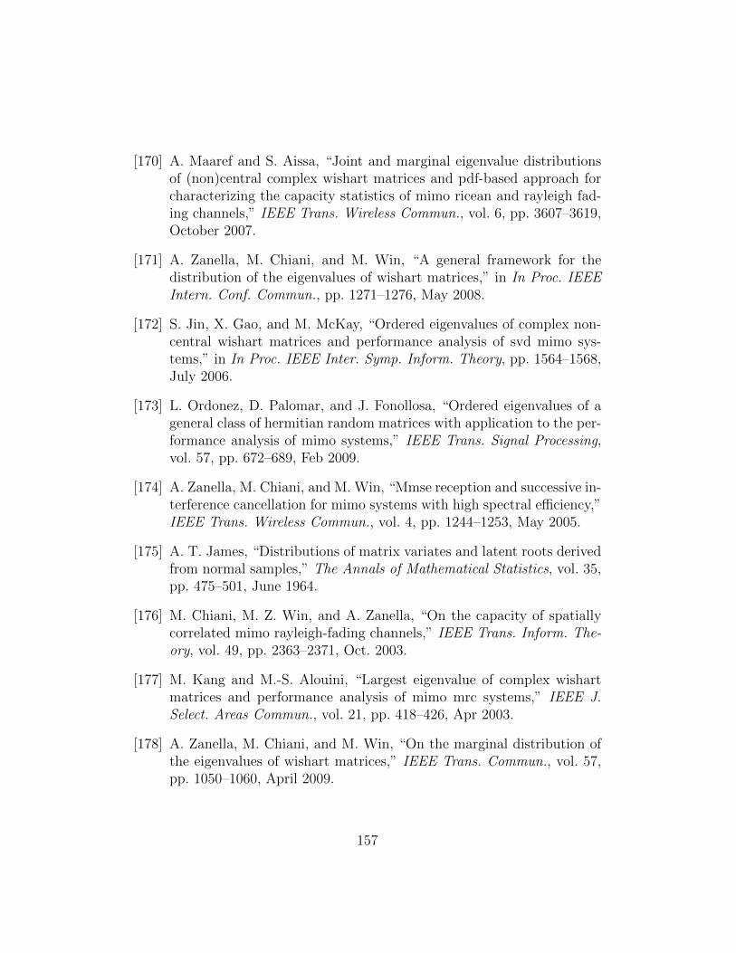
[170] A. Maaref and S. Aissa, “Joint and marginal eigenvalue distributionsof (non)central complex wishart matrices and pdf-based approach forcharacterizing the capacity statistics of mimo ricean and rayleigh fad-ing channels,” IEEE Trans. Wireless Commun., vol. 6, pp. 3607–3619,October 2007.
[171] A. Zanella, M. Chiani, and M. Win, “A general framework for thedistribution of the eigenvalues of wishart matrices,” in In Proc. IEEEIntern. Conf. Commun., pp. 1271–1276, May 2008.
[172] S. Jin, X. Gao, and M. McKay, “Ordered eigenvalues of complex non-central wishart matrices and performance analysis of svd mimo sys-tems,” in In Proc. IEEE Inter. Symp. Inform. Theory, pp. 1564–1568,July 2006.
[173] L. Ordonez, D. Palomar, and J. Fonollosa, “Ordered eigenvalues of ageneral class of hermitian random matrices with application to the per-formance analysis of mimo systems,” IEEE Trans. Signal Processing,vol. 57, pp. 672–689, Feb 2009.
[174] A. Zanella, M. Chiani, and M. Win, “Mmse reception and successive in-terference cancellation for mimo systems with high spectral efficiency,”IEEE Trans. Wireless Commun., vol. 4, pp. 1244–1253, May 2005.
[175] A. T. James, “Distributions of matrix variates and latent roots derivedfrom normal samples,” The Annals of Mathematical Statistics, vol. 35,pp. 475–501, June 1964.
[176] M. Chiani, M. Z. Win, and A. Zanella, “On the capacity of spatiallycorrelated mimo rayleigh-fading channels,” IEEE Trans. Inform. The-ory, vol. 49, pp. 2363–2371, Oct. 2003.
[177] M. Kang and M.-S. Alouini, “Largest eigenvalue of complex wishartmatrices and performance analysis of mimo mrc systems,” IEEE J.Select. Areas Commun., vol. 21, pp. 418–426, Apr 2003.
[178] A. Zanella, M. Chiani, and M. Win, “On the marginal distribution ofthe eigenvalues of wishart matrices,” IEEE Trans. Commun., vol. 57,pp. 1050–1060, April 2009.
157
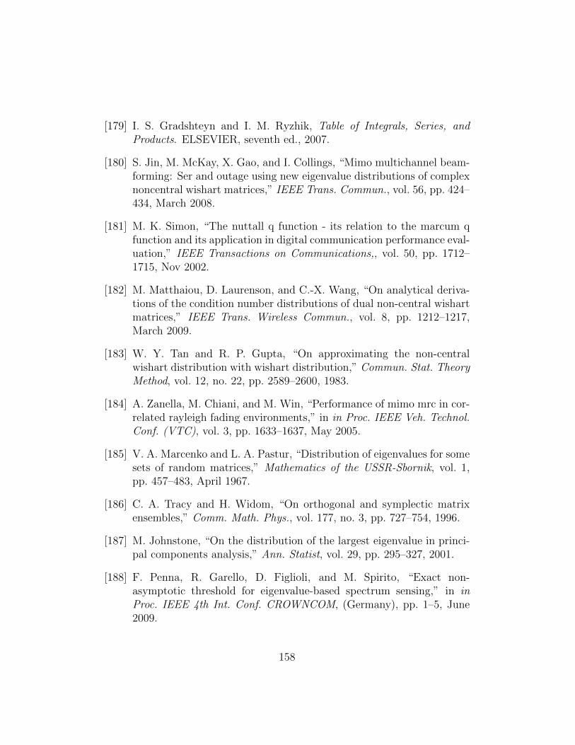
[179] I. S. Gradshteyn and I. M. Ryzhik, Table of Integrals, Series, andProducts. ELSEVIER, seventh ed., 2007.
[180] S. Jin, M. McKay, X. Gao, and I. Collings, “Mimo multichannel beam-forming: Ser and outage using new eigenvalue distributions of complexnoncentral wishart matrices,” IEEE Trans. Commun., vol. 56, pp. 424–434, March 2008.
[181] M. K. Simon, “The nuttall q function - its relation to the marcum qfunction and its application in digital communication performance eval-uation,” IEEE Transactions on Communications,, vol. 50, pp. 1712–1715, Nov 2002.
[182] M. Matthaiou, D. Laurenson, and C.-X. Wang, “On analytical deriva-tions of the condition number distributions of dual non-central wishartmatrices,” IEEE Trans. Wireless Commun., vol. 8, pp. 1212–1217,March 2009.
[183] W. Y. Tan and R. P. Gupta, “On approximating the non-centralwishart distribution with wishart distribution,” Commun. Stat. TheoryMethod, vol. 12, no. 22, pp. 2589–2600, 1983.
[184] A. Zanella, M. Chiani, and M. Win, “Performance of mimo mrc in cor-related rayleigh fading environments,” in in Proc. IEEE Veh. Technol.Conf. (VTC), vol. 3, pp. 1633–1637, May 2005.
[185] V. A. Marcenko and L. A. Pastur, “Distribution of eigenvalues for somesets of random matrices,” Mathematics of the USSR-Sbornik, vol. 1,pp. 457–483, April 1967.
[186] C. A. Tracy and H. Widom, “On orthogonal and symplectic matrixensembles,” Comm. Math. Phys., vol. 177, no. 3, pp. 727–754, 1996.
[187] M. Johnstone, “On the distribution of the largest eigenvalue in princi-pal components analysis,” Ann. Statist, vol. 29, pp. 295–327, 2001.
[188] F. Penna, R. Garello, D. Figlioli, and M. Spirito, “Exact non-asymptotic threshold for eigenvalue-based spectrum sensing,” in inProc. IEEE 4th Int. Conf. CROWNCOM, (Germany), pp. 1–5, June2009.
158
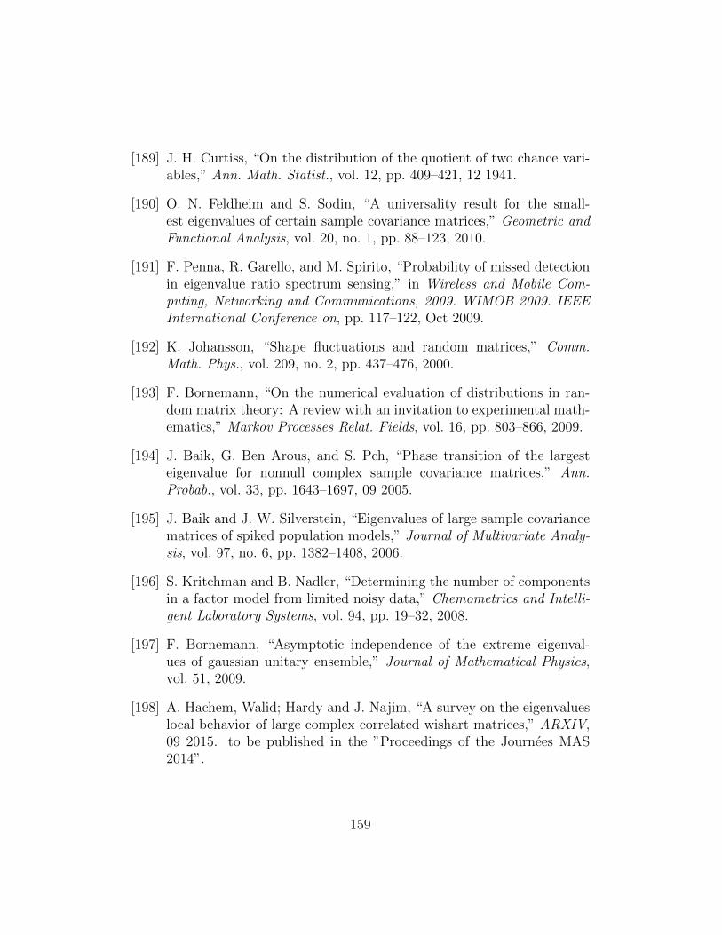
[189] J. H. Curtiss, “On the distribution of the quotient of two chance vari-ables,” Ann. Math. Statist., vol. 12, pp. 409–421, 12 1941.
[190] O. N. Feldheim and S. Sodin, “A universality result for the small-est eigenvalues of certain sample covariance matrices,” Geometric andFunctional Analysis, vol. 20, no. 1, pp. 88–123, 2010.
[191] F. Penna, R. Garello, and M. Spirito, “Probability of missed detectionin eigenvalue ratio spectrum sensing,” in Wireless and Mobile Com-puting, Networking and Communications, 2009. WIMOB 2009. IEEEInternational Conference on, pp. 117–122, Oct 2009.
[192] K. Johansson, “Shape fluctuations and random matrices,” Comm.Math. Phys., vol. 209, no. 2, pp. 437–476, 2000.
[193] F. Bornemann, “On the numerical evaluation of distributions in ran-dom matrix theory: A review with an invitation to experimental math-ematics,” Markov Processes Relat. Fields, vol. 16, pp. 803–866, 2009.
[194] J. Baik, G. Ben Arous, and S. Pch, “Phase transition of the largesteigenvalue for nonnull complex sample covariance matrices,” Ann.Probab., vol. 33, pp. 1643–1697, 09 2005.
[195] J. Baik and J. W. Silverstein, “Eigenvalues of large sample covariancematrices of spiked population models,” Journal of Multivariate Analy-sis, vol. 97, no. 6, pp. 1382–1408, 2006.
[196] S. Kritchman and B. Nadler, “Determining the number of componentsin a factor model from limited noisy data,” Chemometrics and Intelli-gent Laboratory Systems, vol. 94, pp. 19–32, 2008.
[197] F. Bornemann, “Asymptotic independence of the extreme eigenval-ues of gaussian unitary ensemble,” Journal of Mathematical Physics,vol. 51, 2009.
[198] A. Hachem, Walid; Hardy and J. Najim, “A survey on the eigenvalueslocal behavior of large complex correlated wishart matrices,” ARXIV,09 2015. to be published in the ”Proceedings of the Journees MAS2014”.
159
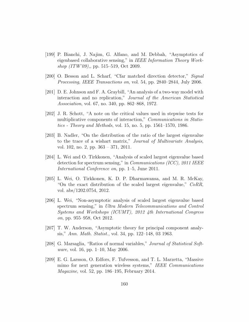
[199] P. Bianchi, J. Najim, G. Alfano, and M. Debbah, “Asymptotics ofeigenbased collaborative sensing,” in IEEE Information Theory Work-shop (ITW’09),, pp. 515–519, Oct 2009.
[200] O. Besson and L. Scharf, “Cfar matched direction detector,” SignalProcessing, IEEE Transactions on, vol. 54, pp. 2840–2844, July 2006.
[201] D. E. Johnson and F. A. Graybill, “An analysis of a two-way model withinteraction and no replication,” Journal of the American StatisticalAssociation, vol. 67, no. 340, pp. 862–868, 1972.
[202] J. R. Schott, “A note on the critical values used in stepwise tests formultiplicative components of interaction,” Communications in Statis-tics - Theory and Methods, vol. 15, no. 5, pp. 1561–1570, 1986.
[203] B. Nadler, “On the distribution of the ratio of the largest eigenvalueto the trace of a wishart matrix,” Journal of Multivariate Analysis,vol. 102, no. 2, pp. 363 – 371, 2011.
[204] L. Wei and O. Tirkkonen, “Analysis of scaled largest eigenvalue baseddetection for spectrum sensing,” in Communications (ICC), 2011 IEEEInternational Conference on, pp. 1–5, June 2011.
[205] L. Wei, O. Tirkkonen, K. D. P. Dharmawansa, and M. R. McKay,“On the exact distribution of the scaled largest eigenvalue,” CoRR,vol. abs/1202.0754, 2012.
[206] L. Wei, “Non-asymptotic analysis of scaled largest eigenvalue basedspectrum sensing,” in Ultra Modern Telecommunications and ControlSystems and Workshops (ICUMT), 2012 4th International Congresson, pp. 955–958, Oct 2012.
[207] T. W. Anderson, “Asymptotic theory for principal component analy-sis,” Ann. Math. Statist., vol. 34, pp. 122–148, 03 1963.
[208] G. Marsaglia, “Ratios of normal variables,” Journal of Statistical Soft-ware, vol. 16, pp. 1–10, May 2006.
[209] E. G. Larsson, O. Edfors, F. Tufvesson, and T. L. Marzetta, “Massivemimo for next generation wireless systems,” IEEE CommunicationsMagazine, vol. 52, pp. 186–195, February 2014.
160

[210] F. Boccardi, R. W. Heath, A. Lozano, T. L. Marzetta, and P. Popovski,“Five disruptive technology directions for 5g,” IEEE CommunicationsMagazine, vol. 52, pp. 74–80, February 2014.
[211] W. H. Chin, Z. Fan, and R. Haines, “Emerging technologies and re-search challenges for 5g wireless networks,” IEEE Wireless Communi-cations, vol. 21, pp. 106–112, April 2014.
[212] C. G. Khatri, “Distribution of the largest or the smallest characteris-tic root under null hypothesis concerning complex multivariate normalpopulations,” Ann. Math. Statist., vol. 35, pp. 1807–1810, 12 1964.
[213] Y. C. Liang, Y. Zeng, E. C. Y. Peh, and A. T. Hoang, “Sensing-throughput tradeoff for cognitive radio networks,” IEEE Transactionson Wireless Communications, vol. 7, pp. 1326–1337, April 2008.
[214] E. Ahmed, A. M. Eltawil, and A. Sabharwal, “Rate gain region and de-sign tradeoffs for full-duplex wireless communications,” IEEE Transac-tions on Wireless Communications, vol. 12, pp. 3556–3565, July 2013.
[215] E. Bjrnson, M. Kountouris, and M. Debbah, “Massive mimo and smallcells: Improving energy efficiency by optimal soft-cell coordination,”in Telecommunications (ICT), 2013 20th International Conference on,pp. 1–5, May 2013.
[216] M. Chiani, M. Win, and H. Shin, “Capacity of mimo systems in thepresence of interference,” in In Proc. IEEE GLOBECOM, (San Fran-cisco), pp. 1–6, Nov 2006.
[217] R. A. Horn and C. R. Johnson, Matrix Analysis. Cambridge UniversityPress, 2nd ed., Oct 2012.
[218] S. Kotz and S. Nadarajah, Extreme Value Distributions: Theory andApplications. Imperial College Press, 2000.
[219] G. Muraleedharan, C. G. Soares, and C. Lucas, Characteristic and Mo-ment Generating Functions of Generalised Extreme Value Distribution(GEV), ch. 14, pp. 269–276. Nova Science, 2011.
161