central difference solutions of the kinematic model of ...€¦polydisperse suspensions and...

Journal of Engineering Mathematics 41: 167–187, 2001.© 2001 Kluwer Academic Publishers. Printed in the Netherlands.

Central difference solutions of the kinematic model of settling ofpolydisperse suspensions and three-dimensional particle-scalesimulations

R. BÜRGER, K.-K. FJELDE1, K. HÖFLER2 and K. HVISTENDAHL KARLSEN3

1Institute of Mathematics A, University of Stuttgart, Pfaffenwaldring 57, 70569 Stuttgart, Germany([email protected])1RF-Rogaland Research, Thormøhlensgt. 55, N-5008 Bergen, Norway ([email protected])2Institute for Computer Applications 1, University of Stuttgart, Pfaffenwaldring 27, 70569 Stuttgart, Germany([email protected])3Department of Mathematics, University of Bergen, Johs. Brunsgt. 12, N-5008 Bergen, Norway([email protected])

Received 11 April 2000; accepted in revised form 13 September 2000

Abstract. The extension of Kynch’s kinematic theory of sedimentation of monodisperse suspensions to poly-disperse mixtures leads to a nonlinear system of conservation laws for the volume fractions of each species.In this paper, we show that a second-order central (Riemann-solver-free) scheme for the solution of systems ofconservation laws can be employed as an efficient tool for the simulation of the settling and the separation ofpolydisperse suspensions. This is demonstrated by comparison with a published experimental study of the settlingof a bidisperse suspension. In addition, we compare the prediction of the one-dimensional kinematic sedimentationmodel with a three-dimensional particle-scale simulation.

Key words: Central difference scheme, particle-scale simulation, polydisperse suspension, sedimentation, systemof conservation laws.

1. Introduction

Mathematical models for the settling of suspensions are of great theoretical and practicalinterest in numerous applications such as mineral processing [1], wastewater treatment [2]and blood centrifugation [3]. A well-known theory of one-dimensional sedimentation of idealsuspensions [4] is due to Kynch [5]. The essential assumption of this kinematic theory is thatthe solid-fluid relative velocity, or slip velocity, is a given function of the local volumetricsolids concentration. The local solids mass balance then turns into a scalar conservation law.While Kynch’s model and its extension to flocculated monodisperse suspensions are wellunderstood now and have been validated for numerous real materials (see [1] for details), mostimplications of kinematic models for polydisperse suspensions (with particles differing in sizeor density) still remain to be explored. Exact entropy weak solutions, even of the apparentlysimple problem of settling of a bidisperse, initially homogeneous suspension, have not yetbeen determined, due to the nonlinear character of the system of the two first-order partialdifferential equations involved. However, as we will show here, modern entropy-satisfyingshock capturing numerical schemes can be successfully employed to solve this problem.

Although there is a large list of authors who have proposed extensions of Kynch’s theoryto the polydisperse case (see [6] for an overview), only a few of them have embedded their

168 R. Bürger et al.

equations in the appropriate mathematical framework of nonlinear systems of conservationlaws [7, 8]. The essential property of solutions of these systems is the formation of disconti-nuities, which appear here in the concentrations of the different particle species. The presenceof discontinuities requires the concept of weak solutions, which are not unique. Thus, anadditional selection principle or entropy condition is necessary to determine the physicallyrelevant weak solution, the entropy weak solution. Discontinuities of entropy weak solutionsare called shocks.

Consequently, it is a desirable property of any numerical scheme suitable for the solutionof the kinematic model of sedimentation of polydisperse suspensions to approximate the en-tropy weak solution, and to detect shocks automatically. Such schemes, which will produceaccurate approximations of discontinuous solutions without explicitly using jump conditionsand shock tracking techniques, are called shock-capturing. The last three decades have seentremendous progress in the development of shock-capturing schemes for nonlinear systems ofconservation laws. We refer, among others, to the books [9, 10, 11] (see also the lecture notes[12]) for a concise introduction to these schemes.

Unfortunately, shock-capturing schemes have so far seldom been employed to sedimenta-tion problems. This may in part be due to the fact that mathematical problems related to theanalysis of the systems of equations arising from the kinematic approach are far from beingwell understood. On the other hand, we believe that researchers, for example in chemical engi-neering, assume the difficulties associated with the presence of shocks to be much greater thanthey actually are, and instead of solving the conservation equations, they construct solutionsof settling problems, e.g., by assuming that the suspension forms a finite number of zones inwhich the settling velocities of each particle species are constant. A typical view seems to bethat expressed by Stamatakis and Tien [13, p. 115]:

The particle concentration profiles, in principle, can be found from the solution of theconservation equations of particles of the various types, applying appropriate initial andboundary conditions. The numerical effort involved in solving conservation equations isoften excessive (with the main difficulty being the need of adequately taking care of themoving-boundary nature of the suspension/sediment interface). Therefore, it is impracticalto examine the dynamics of batch sedimentation using this approach...

In this paper, we show that batch sedimentation can easily and, in our view, efficiently beexamined by a shock-capturing scheme.

Roughly speaking, the shock-capturing schemes may be classified into two categories: cen-tral schemes and upwind schemes. The main disadvantage of upwind schemes is the difficultyof solving the Riemann problem exactly or approximately, especially for complex systemsof conservation laws. We point out that the (exact or approximate) solution of the Riemannproblem for the system of conservation laws that we study in this paper is not known at themoment.

For this reason, we have turned our attention to central schemes. In the 1990s, this class ofschemes has received a considerable amount of (renewed) interest, following Nessyahu andTadmor [14] and their introduction of the second-order sequel to the Lax–Friedrichs scheme.We refer to the lecture notes by Tadmor [12] for a general introduction to central schemes andlist of relevant references.

The second-order central schemes can be viewed as a direct extension of the first-orderLax–Friedrichs central scheme, which is known to be robust but at the same time suffers fromexcessive dissipation. To resolve this latter problem, the second order central schemes are

Sedimentation of polydisperse suspensions 169

based on reconstructing, in each time step, a (MUSCL type) piecewise-linear interpolant fromthe cell averages computed in the previous time step. The interpolant is exactly evolved in timeand then projected onto its staggered averages, resulting in the staggered cell averages for thenext time step. To guarantee the non-oscillatory behaviour of the scheme, the reconstructionuses nonlinear limiters. Unlike upwind schemes, central schemes avoid approximate Riemannsolvers, projections along characteristic directions, and the splitting of the flux vector in up-wind and downwind directions. This should in principle make this scheme a good candidatefor solving complex systems of conservation laws such as the system that we consider in thispaper.

In this paper, we shall not use the original central scheme [14] but rather a modified(non-staggered) version introduced recently by Kurganov and Tadmor in [15]. This modifiedcentral scheme has a smaller numerical viscosity and is better suited for nearly steady-statecalculations which are of interest in the simulation of sedimentation processes. We refer toSection 3 for further details.

The rest of this paper is organized as follows: in Section 2, we recall the kinematic modelof settling of polydisperse ideal suspensions, consider two different constitutive approachesfor the slip velocity of each solid species, and derive the respective governing systems ofequations. In Section 3 the central schemes are described in detail. In Section 4 one of theseschemes is applied to two different test cases: first, we consider the settling of a bidispersesuspension of large and small spheres where the parameters are chosen in such a way that ournumerical results can be compared with the experimental and theoretical results of Schneideret al. [16]. Second, we consider a three-dimensional particle-scale simulation of the settlingof a different bidisperse suspension. In the second case, averaging over each horizontal cross-section of the hypothetical settling columns yields concentration profiles for each speciesthat depend only on height, which we compare with the numerical solution of the kinematicmodel with appropriately chosen parameters. Conclusions that can be drawn from this studyare summarized in Section 5.

2. Kinematic model of sedimentation of polydisperse suspensions

For simplicity, we restrict ourselves to an ideal suspension of a fluid with spherical particlesof N species of different radii r1 > r2 > · · · > rN (see [6] for the general case in which theparticles are also allowed to have different densities). If we denote by vi and φi = φi(x, t) thephase velocity and the local volumetric concentration of particle species i, respectively, themass balances for the solids can be written as

∂φi

∂t+ ∂fi

∂x= 0, i = 1, . . . , N, (1)

where fi = φivi . These balances lead to a solvable system of N scalar equations if either thesolid phase velocities vi or the solid-fluid relative velocities ui = vi − vf, where vf denotesthe fluid-phase velocity, are given as functions of φ1 to φN . The former approach is due toBatchelor and Wen [17, 18], while the latter has been advocated by Masliyah [20]; see alsoBürger et al. [6] and Concha et al. [7].

In both cases, we see that the settling of a polydisperse suspension in a column of heightL can be described by a system of N conservation laws

∂�

∂t+ ∂f(�)

∂x= 0, 0 ≤ x ≤ L, t > 0; f(�) = (

f1(�), . . . , fN(�))T, (2)


where � = (φ1, . . . ,φN)T denotes the vector of concentration values, together with pre-

scribed initial concentrations

φi(x, 0) = φ0i (x), 0 ≤ x ≤ L; 0 ≤ φ0

1(x)+ · · · + φ0N(x) ≤ φmax, (3)

and the zero flux conditions

f|x=0 = 0, f|x=L = 0. (4)

It is well known that solutions of Equation (2) are discontinuous in general. The propaga-tion speed of a discontinuity in the concentration field φi is given by the Rankine-Hugoniotcondition

σi(�+,�−) := fi(�

+)− fi(�−)φ+i − φ−

i

, i = 1, . . . , N, (5)

where �+, φ+i , �− and φ−

i denote the limits of � and φ above and below the discontinuity,respectively. This condition can readily be derived from first principles by considering theflows to and from the interface.

2.1. BATCHELOR’S EQUATION

Batchelor showed that, in a dilute suspension, the phase velocity of spheres of species i isgiven by the expression

vi = vi(�) = u∞i(

1 +N∑j=1

Sijφj

), (6)

where u∞i denotes the Stokes settling velocity of a single particle of radius ri in pure fluid ofdensity �f and dynamic viscosity µf,

u∞i = −2��gr2i

9µf, i = 1, . . . , N; �� = �s − �f, (7)

and the coefficients

Sij = −3.52 − 1.04rj

ri− 1.03

r2j

r2i

, i, j = 1, . . . , N

are given by a fit to data from Batchelor and Wen [18], which in turn represent numericalevaluations of integrals derived [17], i.e., the coefficients Sij are deduced from first principles.

In order to make vi = 0 when the cumulative solids concentration φ := φ1 + · · · + φNattains a maximum value φmax, we replace Batchelor’s equation (6) by the expression (see[19])

vi = u∞i exp

( N∑j=1

Sijφj + 2φ

φmax

)(1 − φ

φmax

)2

, (8)

which vanishes for φ = φmax and has the same partial derivatives for � = 0 as (6). Definingthe parameters

µ = −2��gr21

9µf; δi = r2

i

r21

, i = 1, . . . , N, (9)


we obtain

fi(�) = f Bi (�) = µδiφi exp

( N∑j=1

Sijφj + 2φ

φmax

)(1 − φ

φmax

)2

. (10)

2.2. MASLIYAH’S APPROACH

While formula (6) is based on a postulate for each solid-species phase velocity, the followingapproach essentially involves constitutive equations for the solid-fluid relative velocities vi −vf, where vf denotes the phase velocity of the fluid.

For batch sedimentation in a closed column, the volume-averaged velocity q := (1−φ)vf+φ1v1 +· · ·+φNvN vanishes, which we can easily see by summing equation Equation (1) overi = 1, . . . , N and by taking into account the continuity equation of the fluid,

∂φ

∂t− ∂

∂x

((1 − φ)vf

) = 0,

and that q = 0 at x = 0. In terms of the relative velocities ui := vi − vf, i = 1, · · · , N , wecan rewrite q = 0 as vf = −(φ1u1 + · · · + φNuN). Noting that fi = φi(ui + vf), we obtain

fi = fi(�) = φi(ui − (φ1u1 + · · · + φNuN)

).

Including in his analysis the momentum equations for each particle species and that of the fluidand using equilibrium considerations, Masliyah [20] derived that the constitutive equation forthe solid-fluid relative velocity ui should be of the type

ui = u∞iV (φ), (11)

where u∞i denotes the Stokes settling velocity of a single particle of species i with respect toa fluid of density �(φ) = φ�s + (1 − φ)�f, i.e.,

u∞i = −2(�s − �(φ))gr2i

9µf= −2(1 − φ)��gr2

i

9µf, i = 1, . . . , N, (12)

and where V (φ) can be chosen as one of the hindered settling functions known in the monodis-perse case, for example as the well-known Richardson and Zaki [21] formula

V (φ) = V RZ(φ) = (1 − φ)n, n > 1, 0 ≤ φ ≤ φmax. (13)

With the parameters µ and δi from (9), we finally obtain

fi(�) = fMi (�) = µ(1 − φ)V (φ)

(φi

N∑j=1

δjφj − δiφi

). (14)


2.3. SPECIAL CASE N = 2

In the case of just two particle species, the system of Equations (2) reduces to

∂

∂t

(φ1

φ2

)+ µ

∂

∂x

((1 − φ

φmax

)2

exp

(2φ

φmax

) (φ1 exp (S11φ1 + S12φ2)

δ2φ2 exp (S21φ1 + S22φ2)

))= 0 (15)

in the case of f1 and f2 given by (10) and to

∂

∂t

(φ1

φ2

)+ µ

∂

∂x

(V (φ)(1 − φ)

(δ2φ1φ2 − φ1(1 − φ1)

φ1φ2 − δ2φ2(1 − φ2)

))= 0 (16)

for f1 and f2 given by (14).

3. Second-order central schemes

We shall solve the system of conservation laws (2) by a second-order shock-capturing schemeintroduced first by Nessyahu and Tadmor [14] and later modified by Kurganov and Tadmor[15]. It is the modified version of the scheme that we use here. To make this paper relativelyself-contained, we shall state, as well as briefly derive, this scheme below, starting with theoriginal scheme [14], and then we proceed by explaining the modifications needed to obtainthe scheme in [15]. The reader may therefore consider this section as a short introduction(primer) to central schemes. We refer to [14, 15] and the lecture notes by Tadmor [12] for amore extensive discussion of central schemes.

To approximate the solution � of (2), we introduce a mesh in the (x, t)-plane where thespatial grid points are denoted by xj and the time levels by tn. We denote the length of thespace and time steps by �x and �t , respectively, i.e., xj = j�x and tn = n�t . We chooseintegers J and N such that J�x = L and N�t = T . Moreover, we let λ = �t/�x. We shallalways assume that �x and �t are related through an appropriate CFL condition [14, 15].

In what follows, we derive briefly the central scheme. In doing so, we do not take intoaccount the boundary conditions in (4), which need special care. The boundary scheme willbe described in detail towards the end of this section.

At time level tn, given the cell averages {�nj = (φn1,j , . . . , φnN,j )

T}, we introduce a piecewise-linear reconstruction �(x, tn),

�(x, tn) =∑j

(�n

j + 1

�x�′j

(x − xj

))χ[xj−1/2, xj+1/2](x), (17)

where �′j = (φ′

1,j , . . . ,φ′N,j )

T is the slope vector defined by

φ′�,j = MM

(θ[φn�,j − φn�,j−1

],

1

2

[φn�,j+1 − φn�,j−1

], θ

[φn�,j+1 − φn�,j

]), (18)

for � = 1, . . . , N and θ ∈ [0, 2]. Here, MM(a, b, c) is the minmod function which equalsmin(a, b, c) if a, b, c > 0, max(a, b, c) if a, b, c < 0, and zero otherwise. In particular, thischoice of slope vector satisfies (see [14])

1

�x�′j = ∂

∂x�(x = xj , tn)+ O(�x),


which ensures second-order accuracy wherever the components of � are smooth. In addition,this choice ensures that the approximation is non-oscillatory.

Now integration of (2) over the space-time volume [xj , xj+1]× [tn, tn+1] yields the follow-

ing exact equation for the cell averages {�n+1j+1/2}:

�n+1j+1/2 := 1

�x

∫ xj+1

xj

�(x, tn+1) dx (19)

= �n

j+1/2 − 1

�x

[∫ tn+1

tn

f(�(xj+1, t)

)dt −

∫ tn+1

tn

f(�(xj , t)

)dt

],

where exact integration of (17) gives

�n

j+1/2 := 1

�x

∫ xj+1

xj

�(x, tn) dx = 1

2

(�n

j + �nj+1

) + 1

8

(�′j −�′

j+1

).

Although the piecewise-linear interpolant �(·, tn)may be discontinuous at the points {xj+1/2},the solution�(·, t ≥ tn) remains smooth near each xj for t ≤ tn+1 provided the CFL conditionλSnmax < 1/2 holds, where Snmax denotes the maximum propagation speed throughout thedomain at time tn.

Thus, the time integrals in (19) only involve smooth integrands and they can be computedwithin second-order accuracy by the mid-point rule:

1

�x

∫ tn+1

tn

f(�(xj , t)) dt ≈ λf(�(xj , tn+1/2)

), (20)

where the point-values at the half-time steps are evaluated by Taylor expansion,

�n+1/2j := �(xj , tn+1/2) ≈ �(xj , tn)+ �t

2

∂

∂t�(xj , t = tn) = �

n

j − λ

2f′j . (21)

Here, the slope vector f′j = (f ′1,j , . . . , f

′N,j )

T is defined by

f ′j,� = MM

(θ[f�

(�n

j

) − f�(�n

j−1

)], (22)

1

2

[f�

(�n

j+1

) − f�(�n

j−1

)], θ

[f�

(�n

j+1

) − f�(�n

j

)]),

for � = 1, . . . , N and θ ∈ [0, 2]. In particular, this choice of slope vector ensures second-orderaccuracy in smooth regions, i.e.,

1

�xf′j = ∂

∂xf(�(x = xj , tn))+ O(�x),

and that the numerical approximation is non-oscillatory, see [14].Summing up, we end up with a scheme that consists of a first-order predictor step followed

by a second-order corrector step:Predictor step:

�n+1/2j = �

n

j − λ

2f′j . (23)


Corrector step:

�n+1j+1/2 = 1

2

(�n

j + �nj+1

) + 1

8

(�′j −�′

j+1

) − λ[f(�n+1/2j+1

) − f(�n+1/2j

)]. (24)

We point out that under a suitable CFL condition (see [14]), the central scheme (23)–(24)is TVD (Total Variation Diminishing) for a scalar equation and thus converges to a weaksolution. Moreover, it satisfies a cell entropy inequality for a scalar equation with strictlyconvex flux function and thus converges to the physically correct solution in this case; see[14] for further details.

We note that although the predictor-corrector scheme (23)–(24) uses staggered grid cells(i.e., cells that alternate every other time step), the modified version of the scheme (see below)uses a non-staggered grid.

Note that if we use piecewise-constant instead of piecewise-linear reconstruction in (17),we recover the staggered version of the Lax–Friedrichs scheme. The good resolution of thesecond-order central scheme is because the numerical dissipation is considerably lower thanin the Lax–Friedrichs scheme, which is due to the use of a second-order MUSCL type recon-struction.

The dissipation in the central scheme (23)–(24) is O((�x)4/�t). Nevertheless, as can beseen from this expression for the dissipation, the central scheme does not admit a semi-discreteversion, i.e., we cannot send �t to zero for fixed �x. Hence the scheme is not appropriate forsmall time-step calculations or steady-state calculations as t → ∞. However, the latter areimportant in the context of sedimentation processes. In a previous paper [6], we applied thecentral scheme to the kinematic sedimentation model (2), and indeed it turned out that thisscheme yielded diffusive results for the (nearly) steady-state examples (see [6] for furtherdetails).

Next we describe a modification of the central scheme proposed by Kurganov and Tadmor[15] which reduces the dissipation to O(�x3) and hence makes the scheme better suited forsteady-state calculations. In particular, this scheme remains second-order accurate indepen-dent of O(1/�t) and, letting �t → 0, one obtains even a semi-discrete central scheme. Thebasic idea behind the modified central scheme is to use more accurate information about thelocal speed of propagation of the discontinuities.

Assume that we have reconstructed a piecewise-linear interpolant (17) from the cell av-erages {�nj } at time tn. We then estimate the local propagation speeds {anj+1/2} at the cellboundaries {xj+1/2}. To this end, let

�−j+1/2 := �(xj+1/2−, tn) = �

n

j +�′j /2,

�+j+1/2 := �(xj+1/2+, tn) = �

n

j+1 −�′j+1/2

be the left and right intermediate values of the interpolant �(x, tn) at x = xj+1/2. We thendefine the local speed of propagation

anj+1/2 = max

{ρ( ∂f∂�

(�−j+1/2

)), ρ

( ∂f∂�

(�+j+1/2

))}, (25)

where ρ(A) := max |µi(A)| and {µi(A)} are the eigenvalues of A.Although it is possible (and sometimes necessary) to use “approximate eigenvalues” here,

we have used in this paper the analytical expressions for the eigenvalues to compute the localspeeds {anj+1/2}.


Given the piecewise-linear interpolant �(·, tn) defined in (17) and the local speeds {anj+1/2},the construction of the cell averages {�n+1

j } at time tn+1 proceeds in two steps:

Step 1. The original central scheme is based on averaging over the (staggered) control vol-ume [xj , xj+1] of fixed size �x. Instead, let us integrate over the narrower (and non-uniform)control volume

[xnj+1/2,l, x

nj+1/2,r

] ⊂ [xj , xj+1], where

xnj+1/2,l = xj+1/2 − anj+1/2�t, xnj+1/2,r = xj+1/2 + anj+1/2�t.

For t ≤ tn+1, the solution �(·, t ≥ tn) of (2) with piecewise-linear initial data (17) prescribedat t = tn can be non-smooth only inside the control volume [xnj+1/2,l, x

nj+1/2,r] of width

�xnj+1/2 := xnj+1/2,r − xnj+1/2,l = 2anj+1/2�t.

As in (19), we proceed with exact evaluation of the new cell averages

{ n+1j+1/2 = (

ψn+11,j+1/2, . . . , ψ

n+1N,j+1/2

)T}at tn+1, which yields

n+1j+1/2 := 1

�xnj+1/2

∫ xnj+1/2,r

xnj+1/2,l

�(x, tn+1) dx = �n

j + �nj+1

2+ 1 − anj+1/2λ

4

(�′j −�′

j+1

)

− 1

2anj+1/2�t

[∫ tn+1

tn

f(�(xnj+1/2,r, t)

)dt −

∫ tn+1

tn

f(�(xnj+1/2,l, t)

)dt

].

As we did in (20), using the mid-point rule to approximate the time integrals enables us towrite

n+1j+1/2 = �

n

j + �nj+1

2+ 1 − anj+1/2λ

4

(�′j −�′

j+1

)

− 1

2anj+1/2

[f(�n+1/2j+1/2,r

) − f(�n+1/2j+1/2,l

)], (26)

where the mid-point values are obtained by Taylor expansions (similar to what we did in (21)):

�n+1/2j+1/2,l = �nj+1/2,l −

λ

2f(�nj+1/2,l

)′,

�nj+1/2,l = �n

j +�′j

(1/2 − λanj+1/2

),

�n+1/2j+1/2,r = �nj+1/2,r − λ

2f(�nj+1/2,r

)′,

�nj+1/2,r = �n

j+1 −�′j+1

(1/2 − λanj+1/2

), (27)

where the slope vectors f(�nj+1/2,l

)′, f

(�nj+1/2,r

)′are defined (with obvious changes) as in

(22).Similarly, let

�xnj = xnj+1/2,l − xnj−1/2,r = �x −�t(anj−1/2 + anj+1/2)


denote the width of the (narrow) interval [xnj−1/2,r, xnj+1/2,l] around xj (which is free of neigh-

bouring Riemann fans). As before, integrating exactly and then approximating the resulting(two) time integrals by the mid-point rule, we get the following equation for cell averages{ n+1

j = (ψn+11,j , . . . , ψ

n+1N,j )

T} :

n+1j := 1

�xnj

∫ xnj+1/2,l

xnj−1/2,r

�(x, tn+1) dx

= �n

j − λ

2

(anj+1/2 − anj−1/2

)�′j

− λ

1 − λ(anj−1/2 + anj+1/2

)[f(�n+1/2j+1/2,l

) − f(�n+1/2j−1/2,r

)], (28)

where �n+1/2j+1/2,l and �n+1/2

j−1/2,r are defined in (27).

Step 2. In the second (and final) step, we convert the non-uniform cell averages { n+1j },

{ n+1j+1/2} into cell averages over the non-staggered grid cells

{[xj−1/2, xj+1/2]}. To this end,

we consider a piecewise-linear reconstruction over the non-uniform grid cells at time tn+1 andthen we project its averages onto the original grid. The required piecewise-linear reconstruc-tion takes the form

(x, tn+1) =∑j

( n+1j+1/2 + ′

j+1/2(x − xj+1/2))χ[xnj+1/2,l, x

nj+1/2,r](x)

+∑j

n+1j χ[xnj−1/2,r, x

nj+1/2,l](x), (29)

where the discrete derivative ′j+1/2 = (ψ′

1,j+1/2, . . . ,ψ′N,j+1/2)

T is defined by

ψ′�,j+1/2 = 2

�xMM

(θ

ψn+1�,j+1/2 − ψn+1

�,j

1 + λ(anj+1/2 − anj−1/2

) , (30)

ψn+1�,j+1 − ψn+1

�,j

2 + λ(2anj+1/2 − anj−1/2 − anj+3/2

) ,

θψn+1�,j+1 − ψn+1

�,j+1/2

1 + λ(anj+1/2 − anj+3/2

)), θ ∈ [0, 2],

for � = 1, . . . , N . Here, one should keep in mind that n+1j and

n+1j+1/2 are averages over grid

cells centered around

x = 12(x

nj−1/2,r + xnj+1/2,l)= 1

2(xj−1/2 + xj+1/2)+ �t

2

(anj−1/2 − anj+1/2

)

and x = xj+1/2, respectively.Note that simple averaging over [xj−1/2, xj+1/2] reduces the accuracy of the (resulting)

scheme to first order. It is therefore necessary to use the piecewise-linear reconstruction (29) inorder to not loose the second-order accuracy in the process of converting the non-uniform cellaverages { n+1

j }, { nj+1/2} into cell averages over the non-staggered cells{[xj−1/2, xj+1/2]

}.


Moreover, note that it is not necessary to reconstruct on the intervals{[xnj−1/2,r, x

nj+1/2,l

]}since the solution is smooth there.

Finally, the cell averages {�n+1j } are obtained by averaging (29):

�n+1j := 1

�x

∫ xj+1/2

xj−1/2

(x, tn+1) dx

= λanj−1/2 n+1j−1/2 + λanj+1/2

n+1j+1/2 + [

1 − λ(anj−1/2 + anj+1/2

)] n+1j

+ �x

2

[(λanj−1/2

)2 ′j−1/2 − (

λanj+1/2

)2 ′j+1/2

], (31)

where n+1j−1/2,

n+1j ,

n+1j+1/2 are defined in (26) and (28).

It is the scheme (31) that is used in the numerical examples presented in this paper, whilethe original central scheme (23)–(24) has been applied to (2) in our previous paper [6]. Fora discussion of the mathematical properties of the modified central scheme (31), we refer to[15] (see also [14]).

Before we can apply (31), it remains to describe the treatment of the boundary conditionsin (4). We apply the interior scheme (31) when the index j runs over 3/2, 5/2, . . . , J − 3/2.Next we present the boundary scheme, i.e., the updating formulas for j = 1/2,J − 1/2. Tothis end, we note that the central scheme (31) can be written in conservative form:

�n+1j = �

n

j − λ[F nj+1/2 − F n

j−1/2

], (32)

where the numerical flux F nj+1/2 is defined as

F nj+1/2 = 1

2

(f(�n+1/2j+1/2,r

) + f(�n+1/2j+1/2,l

)) − 1

2anj+1/2

(�n

j+1 − �nj)

+ 1

4anj+1/2

(1 − λanj+1/2

)(�′j +�′

j+1

) + �x

2λ(anj+1/2

)2 ′j+1/2,

where �n+1/2j+1/2,l, �

n+1/2j+1/2,r are defined in (27); anj+1/2 is defined in (25); �′

j , �′j+1 are defined in

(18); and ′j+1/2 is defined in (30).

Roughly speaking, the boundary treatment consists in setting the numerical fluxes to zeroat the boundaries according to the boundary conditions (4). For j = 1/2 and j = J − 1/2,(32) then reads

�n+11/2 = �

n

1/2 − λF n1 , �

n+1J−1/2 = �

n

J−1/2 + λF nJ−1.

To compute F n1 and F n

J−1, we set respectively �′1/2 = ′

1 = 0 and �′J−1/2 = ′

J−1 = 0.In the numerical calculations shown later, we used 0.6 as the CFL number and 400 grid

cells for the spatial discretization. Moreover, in calculating the numerical derivatives we usedθ = 2.

4. Numerical examples

We consider two different cases of settling of a homogeneous suspension with solid particlesof two different sizes. It is customary to use the radius of the smallest particles as a length


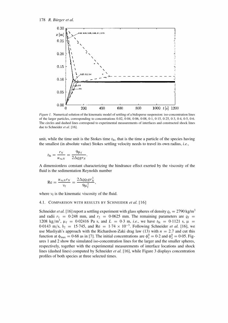
Figure 1. Numerical solution of the kinematic model of settling of a bidisperse suspension: iso-concentration linesof the larger particles, corresponding to concentrations 0.02, 0·04, 0·06, 0·08, 0·1, 0·15, 0·25, 0·3, 0·4, 0·5, 0·6.The circles and dashed lines correspond to experimental measurements of interfaces and constructed shock linesdue to Schneider et al. [16].

unit, while the time unit is the Stokes time tSt, that is the time a particle of the species havingthe smallest (in absolute value) Stokes settling velocity needs to travel its own radius, i.e.,

tSt = rN

u∞N= 9µf

2��grN.

A dimensionless constant characterizing the hindrance effect exerted by the viscosity of thefluid is the sedimentation Reynolds number

Re = u∞NrNνf

= 2��fgr3N

9µ2f

,

where νf is the kinematic viscosity of the fluid.

4.1. COMPARISON WITH RESULTS BY SCHNEIDER et al. [16]

Schneider et al. [16] report a settling experiment with glass spheres of density �s = 2790 kg/m3

and radii r1 = 0·248 mm, and r2 = 0·0625 mm. The remaining parameters are �f =1208 kg/m3, µf = 0·02416 Pa s, and L = 0·3 m, i.e., we have tSt = 0·1121 s, µ =0·0143 m/s, δ2 = 15·745, and Re = 1·74 × 10−3. Following Schneider et al. [16], weuse Masliyah’s approach with the Richardson-Zaki drag law (13) with n = 2.7 and cut thisfunction at φmax = 0·68 as in [7]. The initial concentrations are φ0

1 = 0·2 and φ02 = 0·05. Fig-

ures 1 and 2 show the simulated iso-concentration lines for the larger and the smaller spheres,respectively, together with the experimental measurements of interface locations and shocklines (dashed lines) computed by Schneider et al. [16], while Figure 3 displays concentrationprofiles of both species at three selected times.


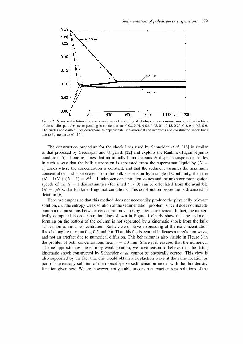
Figure 2. Numerical solution of the kinematic model of settling of a bidisperse suspension: iso-concentration linesof the smaller particles, corresponding to concentrations 0·02, 0·04, 0·06, 0·08, 0·1, 0·15, 0·25, 0·3, 0·4, 0·5, 0·6.The circles and dashed lines correspond to experimental measurements of interfaces and constructed shock linesdue to Schneider et al. [16].

The construction procedure for the shock lines used by Schneider et al. [16] is similarto that proposed by Greenspan and Ungarish [22] and exploits the Rankine-Hugoniot jumpcondition (5): if one assumes that an initially homogeneous N-disperse suspension settlesin such a way that the bulk suspension is separated from the supernatant liquid by (N −1) zones where the concentration is constant, and that the sediment assumes the maximumconcentration and is separated from the bulk suspension by a single discontinuity, then the(N − 1)N + (N − 1) = N2 − 1 unknown concentration values and the unknown propagationspeeds of the N + 1 discontinuities (for small t > 0) can be calculated from the available(N + 1)N scalar Rankine–Hugoniot conditions. This construction procedure is discussed indetail in [6].

Here, we emphasize that this method does not necessarily produce the physically relevantsolution, i.e., the entropy weak solution of the sedimentation problem, since it does not includecontinuous transitions between concentration values by rarefaction waves. In fact, the numer-ically computed iso-concentration lines shown in Figure 1 clearly show that the sedimentforming on the bottom of the column is not separated by a kinematic shock from the bulksuspension at initial concentration. Rather, we observe a spreading of the iso-concentrationlines belonging to φ1 = 0·4, 0·5 and 0·6. That this fan is centred indicates a rarefaction wave,and not an artefact due to numerical diffusion. This behaviour is also visible in Figure 3 inthe profiles of both concentrations near x = 50 mm. Since it is ensured that the numericalscheme approximates the entropy weak solution, we have reason to believe that the risingkinematic shock constructed by Schneider et al. cannot be physically correct. This view isalso supported by the fact that one would obtain a rarefaction wave at the same location aspart of the entropy solution of the monodisperse sedimentation model with the flux densityfunction given here. We are, however, not yet able to construct exact entropy solutions of the


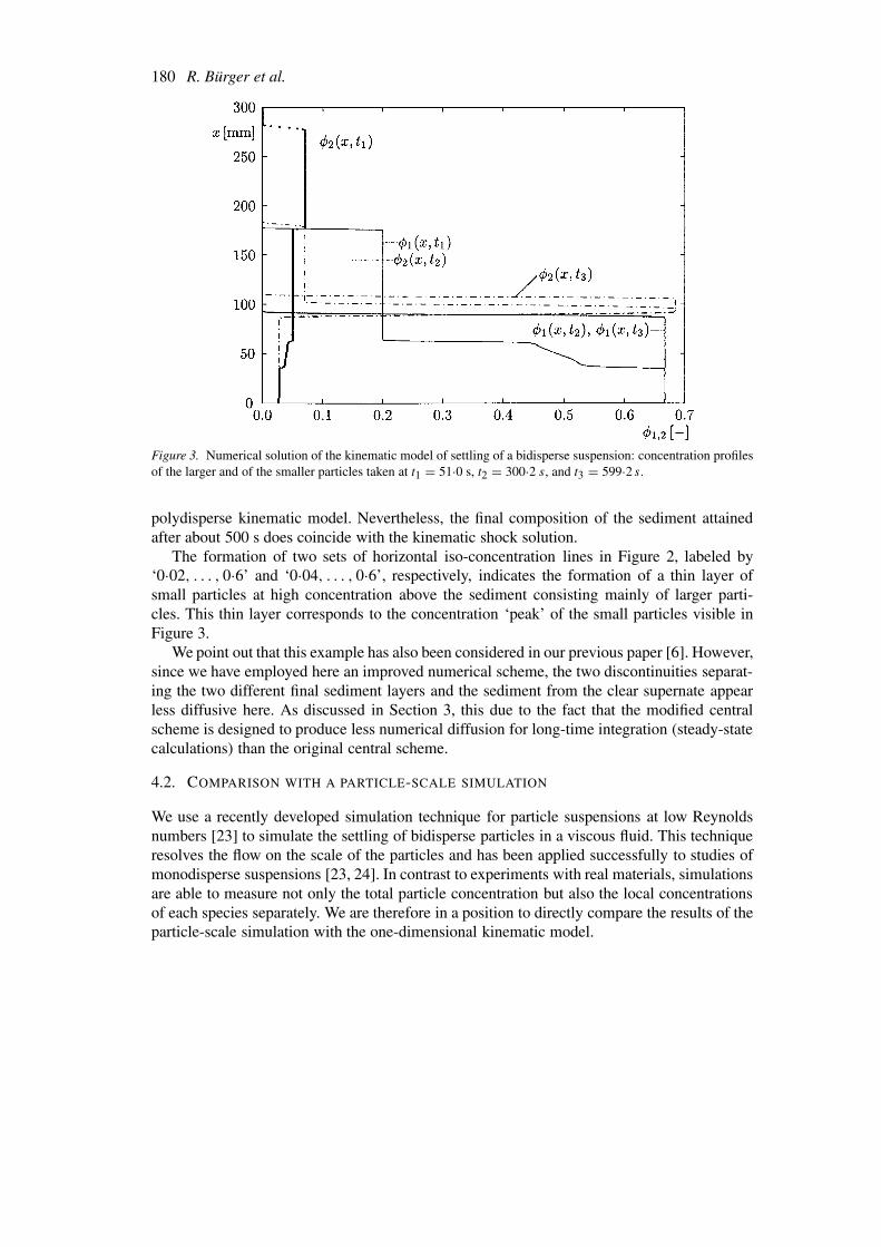
Figure 3. Numerical solution of the kinematic model of settling of a bidisperse suspension: concentration profilesof the larger and of the smaller particles taken at t1 = 51·0 s, t2 = 300·2 s, and t3 = 599·2 s.

polydisperse kinematic model. Nevertheless, the final composition of the sediment attainedafter about 500 s does coincide with the kinematic shock solution.

The formation of two sets of horizontal iso-concentration lines in Figure 2, labeled by‘0·02, . . . , 0·6’ and ‘0·04, . . . , 0·6’, respectively, indicates the formation of a thin layer ofsmall particles at high concentration above the sediment consisting mainly of larger parti-cles. This thin layer corresponds to the concentration ‘peak’ of the small particles visible inFigure 3.

We point out that this example has also been considered in our previous paper [6]. However,since we have employed here an improved numerical scheme, the two discontinuities separat-ing the two different final sediment layers and the sediment from the clear supernate appearless diffusive here. As discussed in Section 3, this due to the fact that the modified centralscheme is designed to produce less numerical diffusion for long-time integration (steady-statecalculations) than the original central scheme.

4.2. COMPARISON WITH A PARTICLE-SCALE SIMULATION

We use a recently developed simulation technique for particle suspensions at low Reynoldsnumbers [23] to simulate the settling of bidisperse particles in a viscous fluid. This techniqueresolves the flow on the scale of the particles and has been applied successfully to studies ofmonodisperse suspensions [23, 24]. In contrast to experiments with real materials, simulationsare able to measure not only the total particle concentration but also the local concentrationsof each species separately. We are therefore in a position to directly compare the results of theparticle-scale simulation with the one-dimensional kinematic model.


4.2.1. Simulation techniqueThe fluid motion is represented by the incompressible Navier-Stokes equations,

∂vf

∂t+ (vf · ∇)vf = −∇p + 1

Re∇2vf + f l , (33)

∇ · vf = 0, (34)

where vf is the fluid velocity measured in units of some typical velocity U , Re = aU/ν is theparticle Reynolds number, a the radius of the spherical particles considered, and ν the dynamicviscosity of the fluid. The pressure p is measured in units of �fU

2,where �f is the fluid density.The point force f l usually represents body forces like gravity, but local force distributions maybe used to model boundary conditions as well (see below). It is convenient to eliminate gravityfrom the equations since it cancels the induced constant hydrostatic pressure gradient; we thenhave to add buoyancy when we consider the forces acting on particles.

In order to solve the fluid equations (33) and (34), we use a fixed, regular grid — astaggered marker and cell mesh — for a second-order spatial discretization [25]. Moreover,we employ a simple explicit Euler time-stepping for the discretization of Equation (33) andan implicit determination of the pressure in an operator-splitting approach to satisfy the in-compressibility constraint at all times. The resulting pressure Poisson equation is solved bymultigrid techniques. For more details, see [25, 26].

Physically, the suspended particles are moving boundaries in the Navier-Stokes equationwhich are not easy to represent. We therefore use the point force term in Equation (33) tomodel the interaction between the fluid and the particles. To this end, we imagine that thephysical particles in the fluid are decomposed as follows. We need (i) a rigid particle templateendowed with a certain mass mti and moment of inertia I ti , which complements (ii) mass andmoment of inertia of the volume Vi of liquid covered — but not replaced — by the template.We must require mti + �fVi = mi and I ti + If = Ii , i.e., that template plus liquid volumeelements together yield the correct mass mi and moment of inertia Ii of the physical particle.

In order to achieve the coupling, we distribute reference points j with coordinates rij overthe particle templates with respect to the center of particle i at xi . These reference points movedue to the translation and rotation of the particle template and follow trajectories xrij (t),

xrij (t) = xi (t)+ Oi(t)rij ,

where Oi(t) is a matrix describing the orientation of the template. Each reference point isassociated with one tracer particle (superscript m) at xmij which is passively advected by theflow field, xmij = vf(xmij ). Whenever the reference point and the tracer are not at the sameposition, forces arise (see below) to make the tracer follow the reference point, i.e., the liquidmotion coincides with the particle motion.

Between a tracer and its reference point we introduce a damped spring which gives rise toa force density in the liquid:

f lij (xmij ) = h−d(−kξij − 2γξij )δ(x

mij ). (35)

In this equation, ξij = xmij − xrij denotes the distance between the tracer and the referencepoint, k is the spring constant, γ is the damping constant, δ(x) the Dirac distribution, and hd

the volume of liquid associated with one marker particle. It should be clear that this force lawis largely arbitrary. We have verified that its choice does not significantly influence the motion


of the physical particle as a whole, provided that k is chosen sufficiently large to ensure thatξij remains always small and the density of markers is about 1/hd [27].

4.2.2. Simulation setupWe consider rigid spheres of radii r1 = 1·41 and r2 = 1·0 in a settling column with cross-section of size (width × height × depth) = 36 × 576 × 36 with walls at the bottom and topand periodic boundary conditions in the other directions. The densities are �f = 1 for the fluidand �s = 2·5 for the particles, and the gravity constant is g = 30. We choose νf = 10 so thatthe Stokes velocities are u∞1 = 2 for the larger and u∞2 = 1 for the smaller particles. Dueto the finite size of the container, the single-particle settling velocity is less than the Stokesvelocity [28]. We account for this effect by scaling the parameter µ in Equation (10) with theappropriate value of 0·85 by substitution of µ with µ′ = 0·85µ.

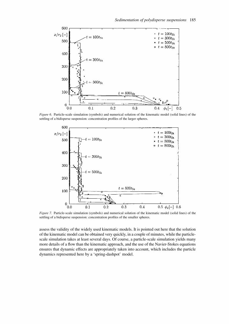
The Reynolds number is Re = 0·1 and tSt = 1. The initial concentrations are φ01 = φ0

2 =0·05. Figures 3 and 4 show the iso-concentration lines for the larger and smaller particles,respectively, obtained from the three-dimensional simulation compared to those determinedby numerical solution of the one-dimensional kinematic model. In Figures 5 and 6, the cor-responding concentration profiles for t = 100tSt, t = 300tSt, t = 500tSt and t = 800tSt arecompared. In the kinematic sedimentation model, we employ the modified Batchelor formula(8). From the given radii, we obtain the coefficients

S11 = S22 = −5·6, S12 = −7·05, S21 = −4·77·The remaining parameters are µ′ = 1·7 and δ2 = 1/2.

4.2.3. Discussion of numerical resultsIn Figures 4 and 5, we compare the iso-concentration lines calculated by numerical solu-tion of the kinematic one-dimensional model with those obtained from the three-dimensionalparticle-scale simulation, while Figures 6 and 7 show the same result as a selection of con-centration profiles. The agreement between the ‘kinematic’ and the ‘particle-scale’ types ofresults visible in these figures indicates that the kinematic model describes fairly well theglobal behaviour of the suspension and predicts correctly the location of fronts.

As a first conclusion, this illustrates that the use of periodic lateral boundary conditions incombination with a global correction of settling velocities in the three-dimensional simulationis the correct way to represent the ‘bulk’ situation, i.e., sedimentation in which all effectsare not appreciable. The importance of this observation lies, of course, in the fact that three-dimensional particle-scale simulations can be performed only in a column of relatively small(compared to the particle size) cross-sectional area.

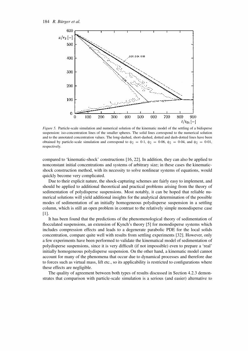
The numerical iso-concentration lines always represent shock lines, i.e. concentration dis-continuities in this example. Their location agrees well with those of the particle-scale ap-proach. This is valid in particular for the interfaces separating the sediment from the super-natant suspension or clear liquid. Moreover, we observe that the kinematic model predicts veryaccurately the thickness and concentration of the thin layer of the smaller particles formingabove the sediment of mixed composition, as visible in Figure 7.

Of course, effects referring to a length scale of particle size such as those described byhydrodynamic diffusion are neglected in the kinematic approach. This becomes apparent inthe smearing of sharp interfaces visible in all figures, and in part in concentration fluctuationsin zones where the kinematic model predicts constant concentrations. A similar spreading ofdiscontinuities by hydrodynamic diffusion is shown in Figure 4 (p. 669) of the very recent


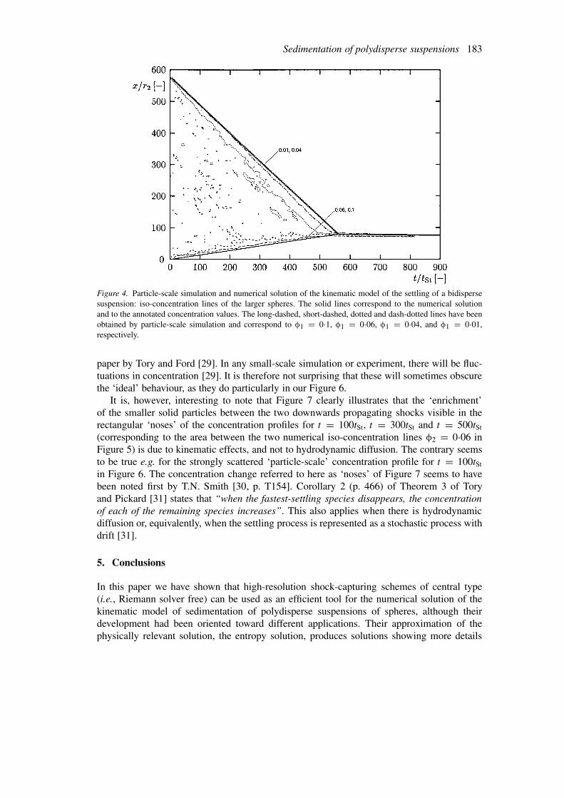
Figure 4. Particle-scale simulation and numerical solution of the kinematic model of the settling of a bidispersesuspension: iso-concentration lines of the larger spheres. The solid lines correspond to the numerical solutionand to the annotated concentration values. The long-dashed, short-dashed, dotted and dash-dotted lines have beenobtained by particle-scale simulation and correspond to φ1 = 0·1, φ1 = 0·06, φ1 = 0·04, and φ1 = 0·01,respectively.

paper by Tory and Ford [29]. In any small-scale simulation or experiment, there will be fluc-tuations in concentration [29]. It is therefore not surprising that these will sometimes obscurethe ‘ideal’ behaviour, as they do particularly in our Figure 6.

It is, however, interesting to note that Figure 7 clearly illustrates that the ‘enrichment’of the smaller solid particles between the two downwards propagating shocks visible in therectangular ‘noses’ of the concentration profiles for t = 100tSt, t = 300tSt and t = 500tSt

(corresponding to the area between the two numerical iso-concentration lines φ2 = 0·06 inFigure 5) is due to kinematic effects, and not to hydrodynamic diffusion. The contrary seemsto be true e.g. for the strongly scattered ‘particle-scale’ concentration profile for t = 100tSt

in Figure 6. The concentration change referred to here as ‘noses’ of Figure 7 seems to havebeen noted first by T.N. Smith [30, p. T154]. Corollary 2 (p. 466) of Theorem 3 of Toryand Pickard [31] states that “when the fastest-settling species disappears, the concentrationof each of the remaining species increases”. This also applies when there is hydrodynamicdiffusion or, equivalently, when the settling process is represented as a stochastic process withdrift [31].

5. Conclusions

In this paper we have shown that high-resolution shock-capturing schemes of central type(i.e., Riemann solver free) can be used as an efficient tool for the numerical solution of thekinematic model of sedimentation of polydisperse suspensions of spheres, although theirdevelopment had been oriented toward different applications. Their approximation of thephysically relevant solution, the entropy solution, produces solutions showing more details


Figure 5. Particle-scale simulation and numerical solution of the kinematic model of the settling of a bidispersesuspension: iso-concentration lines of the smaller spheres. The solid lines correspond to the numerical solutionand to the annotated concentration values. The long-dashed, short-dashed, dotted and dash-dotted lines have beenobtained by particle-scale simulation and correspond to φ2 = 0·1, φ2 = 0·06, φ2 = 0·04, and φ2 = 0·01,respectively.

compared to ‘kinematic-shock’ constructions [16, 22]. In addition, they can also be applied tononconstant initial concentrations and systems of arbitrary size; in these cases the kinematic-shock construction method, with its necessity to solve nonlinear systems of equations, wouldquickly become very complicated.

Due to their explicit nature, the shock-capturing schemes are fairly easy to implement, andshould be applied to additional theoretical and practical problems arising from the theory ofsedimentation of polydisperse suspensions. Most notably, it can be hoped that reliable nu-merical solutions will yield additional insights for the analytical determination of the possiblemodes of sedimentation of an initially homogeneous polydisperse suspension in a settlingcolumn, which is still an open problem in contrast to the relatively simple monodisperse case[1].

It has been found that the predictions of the phenomenological theory of sedimentation offlocculated suspensions, an extension of Kynch’s theory [5] for monodisperse systems whichincludes compression effects and leads to a degenerate parabolic PDE for the local solidsconcentration, compare quite well with results from settling experiments [32]. However, onlya few experiments have been performed to validate the kinematical model of sedimentation ofpolydisperse suspensions, since it is very difficult (if not impossible) even to prepare a ‘real’initially homogeneous polydisperse suspension. On the other hand, a kinematic model cannotaccount for many of the phenomena that occur due to dynamical processes and therefore dueto forces such as virtual mass, lift etc., so its applicability is restricted to configurations wherethese effects are negligible.

The quality of agreement between both types of results discussed in Section 4.2.3 demon-strates that comparison with particle-scale simulation is a serious (and easier) alternative to


Figure 6. Particle-scale simulation (symbols) and numerical solution of the kinematic model (solid lines) of thesettling of a bidisperse suspension: concentration profiles of the larger spheres.

Figure 7. Particle-scale simulation (symbols) and numerical solution of the kinematic model (solid lines) of thesettling of a bidisperse suspension: concentration profiles of the smaller spheres.

assess the validity of the widely used kinematic models. It is pointed out here that the solutionof the kinematic model can be obtained very quickly, in a couple of minutes, while the particle-scale simulation takes at least several days. Of course, a particle-scale simulation yields manymore details of a flow than the kinematic approach, and the use of the Navier-Stokes equationsensures that dynamic effects are appropriately taken into account, which includes the particledynamics represented here by a ‘spring-dashpot’ model.


However, as the preceding brief discussion of ‘enrichment’ of small particles has shown,the solution of a kinematic model with a reliable, i.e. entropy satisfying shock-capturingscheme may help to interpret results obtained from three-dimensional simulations and to drawadditional conclusions from a given simulation, for example which phenomena would persist,even if the ratio of particle size and vessel dimensions tend to zero. Therefore, we believethat the kinematic approach and its particular numerical discretization outlined here are avaluable tool even in applications where the fully three-dimensional particle-scale approachis essential.

Acknowledgements

We acknowledge financial support by the Sonderforschungsbereich 404 at the University ofStuttgart and by the Applied Mathematics in Industrial Flow Problems (AMIF) programme ofthe European Science Foundation (ESF). We would like thank the Norwegian Research Coun-cil for financial support of Kjell Kåre Fjelde and Kenneth Hvistendahl Karlsen through theStrategic Institute Program ‘Complex Wells’; and Professor E.M. Tory for valuable commentsand suggestions.

References

1. M.C. Bustos, F. Concha, R. Bürger and E.M. Tory, Sedimentation and Thickening. Dordrecht: KluwerAcademic Publishers (1999) 304 pp.

2. G.A. Ekama, J.L. Barnard, F.W. Günthert, P. Krebs, J.A. McCorquodale, D.S. Parker and E.J. Wahlberg,Secondary Settling Tanks. London: International Association on Water Quality (1997) 232 pp.

3. W.K. Sartory, Three-component analysis of blood sedimentation by the method of characteristics, Math.Biosci. 33 (1977) 145–165.

4. P.T. Shannon, E. Stroupe and E.M. Tory, Batch and continuous thickening, Ind. Eng. Chem. Fund. 2 (1963)203–211.

5. G.J. Kynch, A theory of sedimentation, Trans. Faraday Soc. 48 (1952) 166–176.6. R. Bürger, F. Concha, K.-K. Fjelde and K.H. Karlsen, Numerical simulation of the settling of polydisperse

suspensions of spheres. Powder Technol. 113 (2000) 30–54.7. F. Concha, C.H. Lee and L.G. Austin, Settling velocities of particulate systems: 8. Batch sedimentation of

polydispersed suspensions of spheres, Int. J. Mineral Process. 35 (1992) 159–175.8. Y.T. Shih, D. Gidaspow and D.T. Wasan, Hydrodynamics of sedimentation of multisized particles, Powder

Technol. 50 (1987) 201–215.9. E. Godlewski and P.-A. Raviart, Numerical Approximation of Hyperbolic Systems of Conservation Laws.

New York: Springer Verlag (1996) 509 pp.10. R. J. LeVeque, Numerical Methods for Conservation Laws. (2nd ed.) Basel: Birkhäuser Verlag (1992) 214 pp.11. E. F. Toro, Riemann Solvers and Numerical Methods for Fluid Dynamics. Berlin: Springer Verlag (1997)

610 pp.12. E. Tadmor, Approximate solutions of nonlinear conservation laws, in A. Quarteroni (ed.), Advanced Numer-

ical Approximation of Nonlinear Hyperbolic Equations, Lecture Notes in Mathematics 1697, 1997 C.I.M.E.Course in Cetraro, Italy, June 1997. Berlin: Springer Verlag (1998) pp. 1–149.

13. K. Stamatakis and C. Tien, Dynamics of batch sedimentation of polydispersed suspensions, Powder Technol.56 (1988) 105–117.

14. H. Nessyahu and E. Tadmor, Nonoscillatory central differencing for hyperbolic conservation laws, J. Comp.Phys. 87 (1990) 408–463.

15. A. Kurganov and E. Tadmor, New high resolution central schemes for nonlinear conservation laws andconvection-diffusion equations, J. Comp. Phys. 160 (2000) 241–282.

16. W. Schneider, G. Anestis and U. Schaflinger, Sediment composition due to settling of particles of differentsizes, Int. J. Multiphase Flow 11 (1985) 419–423.


17. G.K. Batchelor, Sedimentation in a dilute polydisperse system of interacting spheres. Part1. General theory,J. Fluid Mech. 119 (1982) 379–408.

18. G.K. Batchelor and C.S. Wen, Sedimentation in a dilute polydisperse system of interacting spheres. Part 2.Numerical results, J. Fluid Mech. 124 (1982) 495–528.

19. K. Höfler and S. Schwarzer, The structure of bidisperse suspensions at low Reynolds numbers. In: A.-M. Sändig, W. Schiehlen and W.L. Wendland (eds.), Multifield Problems: State of the Art. Berlin: SpringerVerlag (2000) pp. 42–49.

20. J.H. Masliyah, Hindered settling in a multiple-species particle system, Chem. Eng. Sci. 34 (1979) 1166–1168.21. J.F. Richardson and W.N. Zaki, Sedimentation and fluidization I, Trans. Instn. Chem. Engrs. (London) 32

(1954) 35–53.22. H.P. Greenspan and M. Ungarish, On hindered settling of particles of different sizes, Int. J. Multiphase Flow

8 (1982) 587–604.23. K. Höfler and S. Schwarzer, Navier-Stokes simulation with constraint forces: Finite-difference method for

particle-laden flows and complex geometries, Phys. Rev. E 61 (2000) 7146–7160.24. B. Wachmann and S. Schwarzer, Three-dimensional massively parallel computing of suspensions, Int. J.

Mod. Phys. C 9 (1998) 759–775.25. R. Peyret and T. D. Taylor, Computational Methods for Fluid Flow. New York: Springer-Verlag (1983)

338 pp.26. W. Kalthoff, S. Schwarzer and H. Herrmann, Algorithm for the simulation of particle suspensions with inertia

effects. Phys. Rev. E 56 (1997) 2234–2242.27. K. Höfler, Räumliche Simulation von Zweiphasenflüssen. Stuttgart: Diploma Thesis, Institute for Computer

Applications I, University of Stuttgart (1997) 82 pp.28. H. Hasimoto, On the periodic fundamental solutions of the Stokes equations and their application to viscous

flow past a cubic array of spheres, J. Fluid Mech. 5 (1959) 317–328.29. E.M. Tory and R.A. Ford, Stochastic simulation of sedimentation, in M. Rahman and C.A. Brebbia (eds.),

Advances in Fluid Mechanics III. Southampton: WIT Press (2000) 663–672.30. T.N. Smith, The sedimentation of particles having a dispersion of sizes, Trans. Instn. Chem. Engrs. (London)

44 (1966) T153–T157.31. E.M. Tory and D. Pickard, Extensions and refinements of a Markov model of sedimentation, J. Math. Anal.

Appl. 86 (1982) 442–470.32. R. Bürger, F. Concha and F.M. Tiller, Applications of the phenomenological theory to several published

experimental cases of sedimentation processes. Chem. Eng. J. 80 (2000) 105–117.

central difference solutions of the kinematic model of ...€¦polydisperse suspensions and...

Documents