central bank policy impacts on the distribution of future...
TRANSCRIPT
Duke University, Fuqua School of BusinessUniversity of Pennsylvania, Wharton School of Business
Central Bank Policy Impacts on the Distribution of Future Interest Rateson the Distribution of Future Interest Rates
Douglas T. Breeden* and Robert H. Litzenberger**g gSeptember 20, 2013
Notes for presentation at the Federal Reserve Bank of New York/Notes for presentation at the Federal Reserve Bank of New York/New York University Conference on “Risk Neutral Densities”
*William W. Priest Professor of Finance, Duke University, Fuqua School of Business, and Co-Founder and Senior Consultant, Smith Breeden Associates. Email: [email protected] and Website: dougbreeden.net.
**Edward Hopkinson Professor of Investment Banking Emeritus, The Wharton School, University of Pennsylvania.
We thank Robert Merton Robert Litterman Michael Brennan Francis Longstaff David Shimko Stephen Ross andWe thank Robert Merton, Robert Litterman, Michael Brennan, Francis Longstaff, David Shimko, Stephen Ross and Stephen Figlewski for helpful comments and discussions. We thank Lina Ren of Smith Breeden Associates, B.J. Whisler of Harrington Bank, Layla Zhu of MIT and Matthew Heitz of Duke for excellent research assistance. Of course, all remaining errors are our own.

I. State Prices and Risk Neutral Densities Implicit in Prices of InterestDensities Implicit in Prices of Interest
Rate Caps and Floors

Disadvantages of Many Prior Approaches for Estimating Risk Neutral Densitiesg
• 1. Short-term option prices used.Most options mature in 3 months to 18 months, as p ,many markets only have active markets for those maturities. Often there are not options actively traded for a large number of standardized striketraded for a large number of standardized strike prices.
• 2. Parametric vs. nonparametric approach.Applications often parameterize option prices with 3 4 t ( i k3 or 4 parameters (mean, variance, skewness, kurtosis) and estimate implied volatility surfaces and entire risk-neutral densities. It is well-known among practitioners that these methods can be off significantly in estimating tail risks. 3

State Prices Implicit in Interest Rate Cap and Floor PricesInterest Rate Cap and Floor Prices
• Interest rate caps and floors are portfolios of long-term put and call options on 3-month LIBOR No option on first quarter rate so 19options on 3 month LIBOR. No option on first quarter rate, so 19 quarterly options on 5-yr floor, and 11 quarterly options on 3-year floor. Caps and floors are portfolios of long-term options and are traded in large volumes by many portfolio managers and financial i tit ti t h d / ti i kinstitutions to hedge/manage option risk.
• Difference between 5-yr floor price and 4-year floor price is value of 4 quarterly options on LIBOR in year 5 a “floorlet ” Similar for “caplets ”quarterly options on LIBOR in year 5, a floorlet. Similar for caplets.
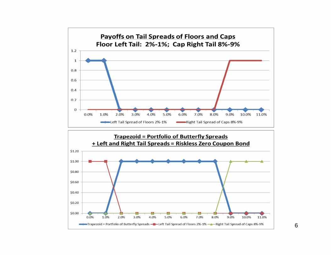
• Approach: Compute butterfly spreads of option prices with various strike rates per Breeden-Litzenberger 1978 to get prices of (trianglesstrike rates, per Breeden-Litzenberger 1978, to get prices of (triangles of) state contingent claims, proportional to the “risk neutral density.”
• Example: Long 1 floor with strike rate of 2% short 2 for 3% long 1 forExample: Long 1 floor with strike rate of 2%, short 2 for 3%, long 1 for 4% gives payoff only between 2% and 4%, peaking at 3%.
4

5
6

Butterfly Spread and Tail Spread Costs and Ri k N t l P b bilitRisk Neutral Probabilites
Figure 6F
Spread Cost “Risk-Neutral Probability”“0%” = Left tail spread: Long 1%, Short 0% floorlet $0.290 0.297 1% Butterfly spread (Long 0%, Short 2 1%, Long 2%) $0.320 0.328 2% Butterfly spread (Long 1%, Short 2 2%, Long 3%) $0.180 0.1843% Butterfly spread $0.080 0.082 4% Butterfly spread $0.037 0.038 5% B fl d $0 028 0 0285% Butterfly spread $0.028 0.0286% Butterfly spread $0.014 0.014 7% Butterfly spread $0.007 0.007 8% B tt fl d $0 007 0 0078% Butterfly spread $0.007 0.0079%+ = Right tail spread: Long 8%, Short 9% caplet $0.015 0.015 Totals $0.977 1.000
7

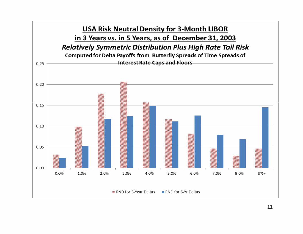
II. Estimates of USA State Prices Implicit in Prices of Interest Rate CapsImplicit in Prices of Interest Rate Caps
and Floors, 2003-2012.

9

10
11

12
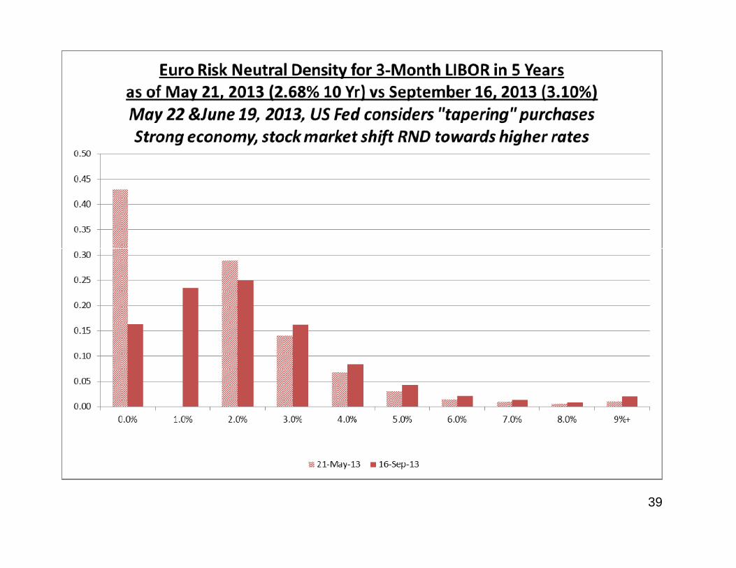
III. Risk Neutral Densities for 6-Month Euro LIBOR from Dec 2003 to Dec 2012
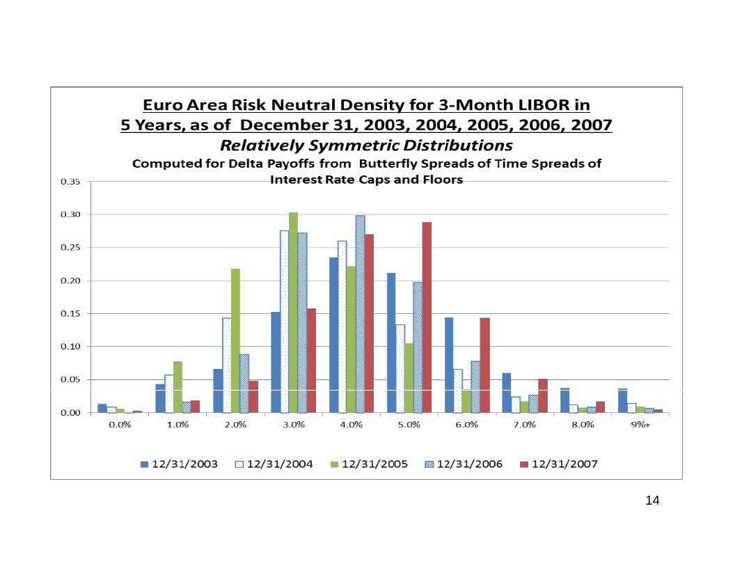
14

15

16

17

IV. Impact of pUSA Federal Reserve Policy
Announcements on State Prices andAnnouncements on State Prices and Risk Neutral Densities for Future
Levels of 3 Month LIBORLevels of 3-Month LIBOR
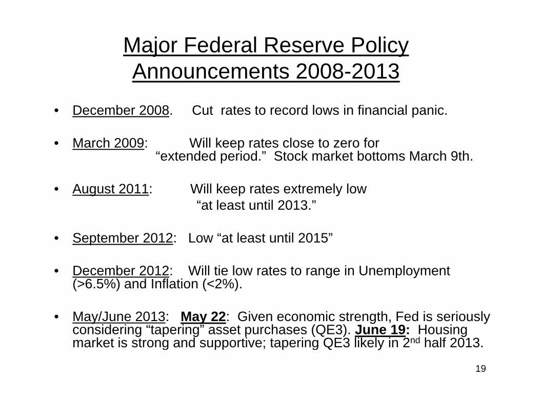
Major Federal Reserve Policy Announcements 2008-2013Announcements 2008 2013
• December 2008. Cut rates to record lows in financial panic.
• March 2009: Will keep rates close to zero for “extended period.” Stock market bottoms March 9th.
• August 2011: Will keep rates extremely low“at least until 2013.”
S t b 2012 L “ t l t til 2015”• September 2012: Low “at least until 2015”
• December 2012: Will tie low rates to range in Unemployment (>6.5%) and Inflation (<2%).( 6.5%) and Inflation ( 2%).
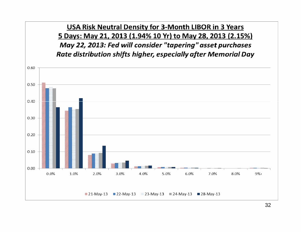
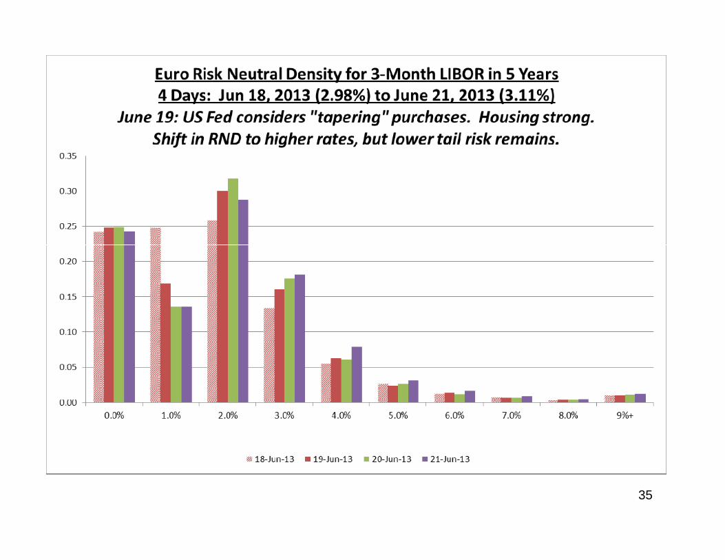
• May/June 2013: May 22: Given economic strength, Fed is seriously considering “tapering” asset purchases (QE3). June 19: Housing market is strong and s pporti e tapering QE3 likel in 2nd half 2013market is strong and supportive; tapering QE3 likely in 2nd half 2013.
19

20
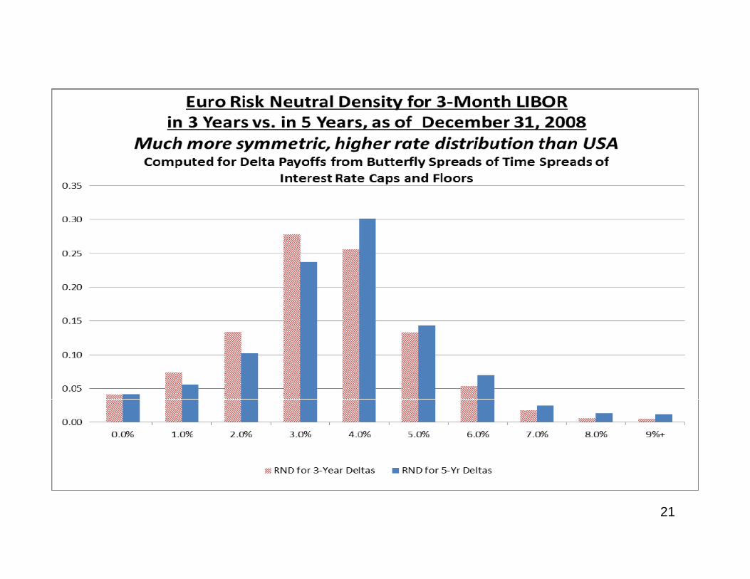
21

22

23

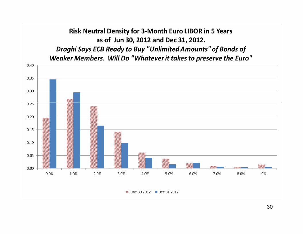
V. Risk Neutral Densities for Euro LIBOR During the Sovereign Debt Crisis 2010-During the Sovereign Debt Crisis 2010
2013

Key Events in the European Sovereign Debt Crisis European Central Bank 2010-2012Crisis European Central Bank 2010 2012
Source: BBC, Reuters• January 2010. Greek deficit revised upward from 3.7% to 12.7%. “Severe
irregularities” in accounting.• April, May 2010, EU agrees to $30 billion, then $110 billion bailout of Greece.
Ireland bailed out in November 2010.
• July 2011: Talk of Greek exit from Euro. Second bailout agreed.• August 2011: European Commission President Barroso warns sovereign
debt crisis spreading. Spain, Italy yields surge.• November 1 2011: Mario Draghi takes over European Central Bank fromNovember 1, 2011: Mario Draghi takes over European Central Bank from
Jean-Claude Trichet. Draghi cuts rates twice quickly.
• July, 2012: ECB cuts rates again.• September 2012: ECB ready to buy “unlimited amounts” of bonds of weaker• September, 2012: ECB ready to buy unlimited amounts of bonds of weaker
member countries. Draghi says ECB will do “whatever it takes to preserve the Euro.” “…and believe me, it will be enough.”
• May/June 2013: U S Fed considers “tapering” asset purchases as economy• May/June 2013: U.S.Fed considers tapering asset purchases, as economy strengthens. Long term interest rates move up sharply.
25

26
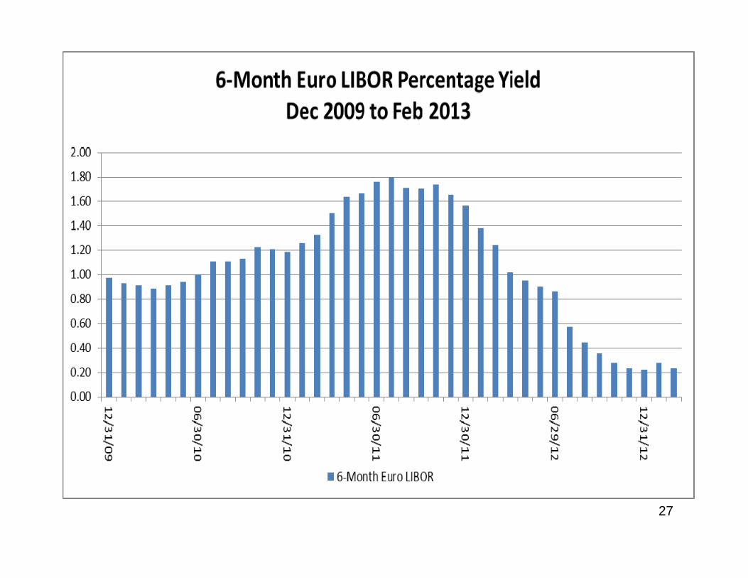
27

28

29
30
VI. May-September 2013U S Federal Reserve ConsidersU.S. Federal Reserve Considers
“Tapering” Asset Purchases
31
32

33

34
35

36

37

38
39

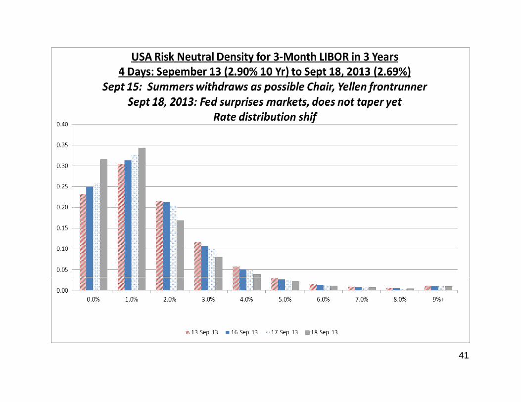
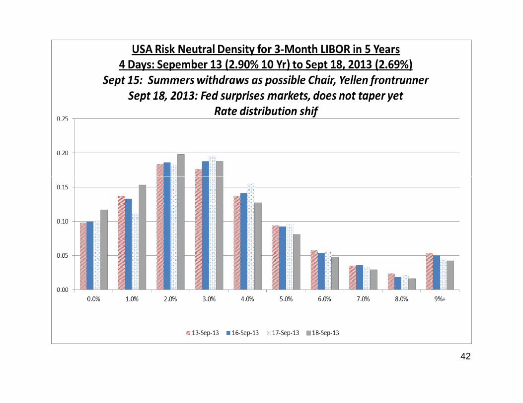
P t i tPostscript:September 15-18, 2013 Events
September 15: Larry Summers withdraws from p yconsideration as new Fed Chair. Janet Yellen presumed frontrunner, believed proponent of easy money longer.
September 18: Fed surprises markets and does not start “taper.” Reduces growth forecasts.
40
41
42

VIII. Conclusions1. The approach of Breeden-Litzenberger 1978 is being used to
estimate tail risks and risk neutral densities in practice.
2. Time spreads of interest rate caps and floors give prices for long-term call and put options (e.g., 4-5 year maturities) on 3-month LIBOR. State prices and risk neutral densities implicit in cap and floor prices are realistic and recently have been highly non normalfloor prices are realistic and recently have been highly non-normal (very positively skewed), as near-zero interest rates occurred.
3. This approach is non-parametric, using only cap and floor prices pp p , g y p pthat are generally observable. No parameter estimation needed.
3. Before and after state prices/risk neutral densities implicit in interest rate floors and caps demonstrate the efficacy (andinterest rate floors and caps demonstrate the efficacy (and sometimes the lack thereof) of Federal Reserve and European Central Bank policy actions on interest rate probability distributions. Distributions have changed shape quite dramatically in the past 10 yearsyears.
43
Appendix 1
R i f Th d R t UR i f Th d R t U
Appendix 1
Review of Theory and Recent Uses:Review of Theory and Recent Uses:Prices of State Contingent Claims Prices of State Contingent Claims
Implicit in Option PricesImplicit in Option Prices
Stephen Ross (Yale/MIT) (1976, QJE), Stephen Ross (Yale/MIT) (1976, QJE), Douglas BreedenDouglas Breeden--Robert Robert LitzenbergerLitzenberger(Stanford/Chicago 1978 J Business)(Stanford/Chicago 1978 J Business)(Stanford/Chicago, 1978, J Business)(Stanford/Chicago, 1978, J Business)
44

State Prices (Arrow Securities) Implicit in Option PricesBreeden-Litzenberger 1978, Journal of Business, following Ross 1976 QJE.
In general, any derivative asset with payoffs )~(Pf can be priced by arbitrage from the prices of $1
“elementary claims” on P~ . An elementary claim on P~has a payoff of $1 contingent upon
.~,~,~21 NPPPPPP === With these, we can price all payoffs of the form )~(Pf .,, 21 N , p p y )(f
The following construction shows that elementary claims can be created from call or put options:
Call Option PortfoliosPayoffs on Call Options Port A Port B Port C=A‐B “ButterflyPayoffs on Call Options Port. A Port. B Port.C=A‐B
P C(X=2) C(X=3) C(X=4) C(2)‐C(3) C(3)‐C(4) C(2)‐2C(3)+C(4)1 0 0 0 0 0 02 0 0 0 0 0 03 1 0 0 1 0 14 2 1 0 1 1 0
ySpreads”of OptionsGive State Prices 4 2 1 0 1 1 0
5 3 2 1 1 1 06 4 3 2 1 1 0. . . . . . .. . . . . . .. . . . . . .
and Risk NeutralDensities
Generally, Δ
Δ+−−−Δ−==
)]()([)]()([)~( xcxcxcxcxPe
N N‐2 N‐3 N‐4 1 1 0
45===
Δ=
→Δ)~()~(lim
0PxcxPe
xx 2nd partial of call price w.r.t. exercise price, evaluated at .~Px =

46
Selected Academic Articles and ExtensionsSelected Academic Articles and Extensions
Articles estimating risk neutral densities and/or applying them to price more complex securitiesapplying them to price more complex securities include academic works by Banz and Miller (1978), Shimko (1993), Rubinstein (1994), Longstaff (1995), Jackwerth and Rubinstein (1996), Ait-Sahalia and Lo (1998), Ait-Sahalia, Wang and Yared (2001),
Longstaff, Santa-Clara and Schwartz (2001), Ait-Sahalia and Duarte (2003), Carr (1998, 2004, 2012) Bates (2000) Li and Zhao (2006) Figlewski2012), Bates (2000), Li and Zhao (2006), Figlewski(2008), Zitzewitz (2009), Birru and Figlewski(20010a,b), Kitsul and Wright (2012), Ross (2013),
47
and Martin (2013), to name a few.
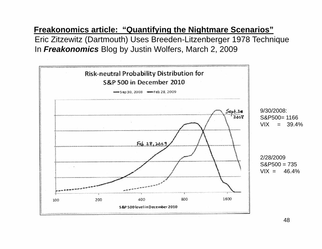
Freakonomics article: “Quantifying the Nightmare Scenarios”Eric Zitzewitz (Dartmouth) Uses Breeden-Litzenberger 1978 Technique
f 2 2009In Freakonomics Blog by Justin Wolfers, March 2, 2009
9/30/20089/30/2008:S&P500= 1166VIX = 39.4%
2/28/2009S&P500 = 735VIX = 46 4%VIX = 46.4%
48

Central Bank ApplicationsCentral banks have also estimated “option implied (risk-Central banks have also estimated option implied (riskneutral) probability distributions” using these techniques. Central bank applications are discussed in articles of B h (1996 1997) Cl P i i t l dBahra (1996, 1997), Clews, Panigirtzoglous and Proudman (2000), and Smith (2012) of the Bank of England,; Malz (1995,1997) of the Federal Reserve Board of New York; and Durham (2007) and Kim (2008) of the Federal Reserve Bank of Washington.
Kocherlakota’s (2013) research group at the Federal Reserve Bank of Minneapolis use Shimko’s (1993) statistical method applying the Breeden Litzenbergerstatistical method applying the Breeden-Litzenbergerformula to regularly estimate and publish RNDs and tail risks (e.g., risk neutral probabilities of moves of +/- 20% or
49
more) for many assets, such as stocks, crude oil, wheat, real estate, and foreign exchange.

Federal Reserve Bank of Minneapolis Uses Breeden-Litzenberger Method to Estimate “Tail Risk” Every 2
W k F St k C diti C i R l E t tWeeks For Stocks, Commodities, Currencies, Real Estate.
50Source: Excerpts from “Methodology” tab of Federal Reserve Bank of Minneapolis
website, February 1, 2013. President: Dr. Narayana Kocherlakota.

51

European Central Bank ArticleECB Monthly Bulletin, February 2011C o t y u et , eb ua y 0Distributions for Euribor in 3 Months
52

European Central Bank Article (cont.)ECB Monthly Bulletin, February 2011C o t y u et , eb ua y 0Distributions for Euribor in 3 Months
53

Appendix 2
True Probabilities vs. Risk Neutral ProbabilitiesRisk Neutral Probabilities (Normalized State Prices)

In a general state preference model:In a general state preference model: Inserting eq. 6 for the zero coupon bond gives:
[ ]]~[
~*
t
jts
tr uEruE
j
jtr
′
′=
π
φ (12)
j
Thus, we see that the risk-neutral probability to true probability ratio at the optimum for rj is
equal to the expected marginal utility of consumption, conditional upon the interest rate being at
the specified level, divided by the unconditional expected marginal utility of consumption at time
t. So if we are looking at butterfly spreads or digital options centered upon LIBOR = 2%, we
need to compute the conditionally expected marginal utility of consumption, given that 2% rate.
55
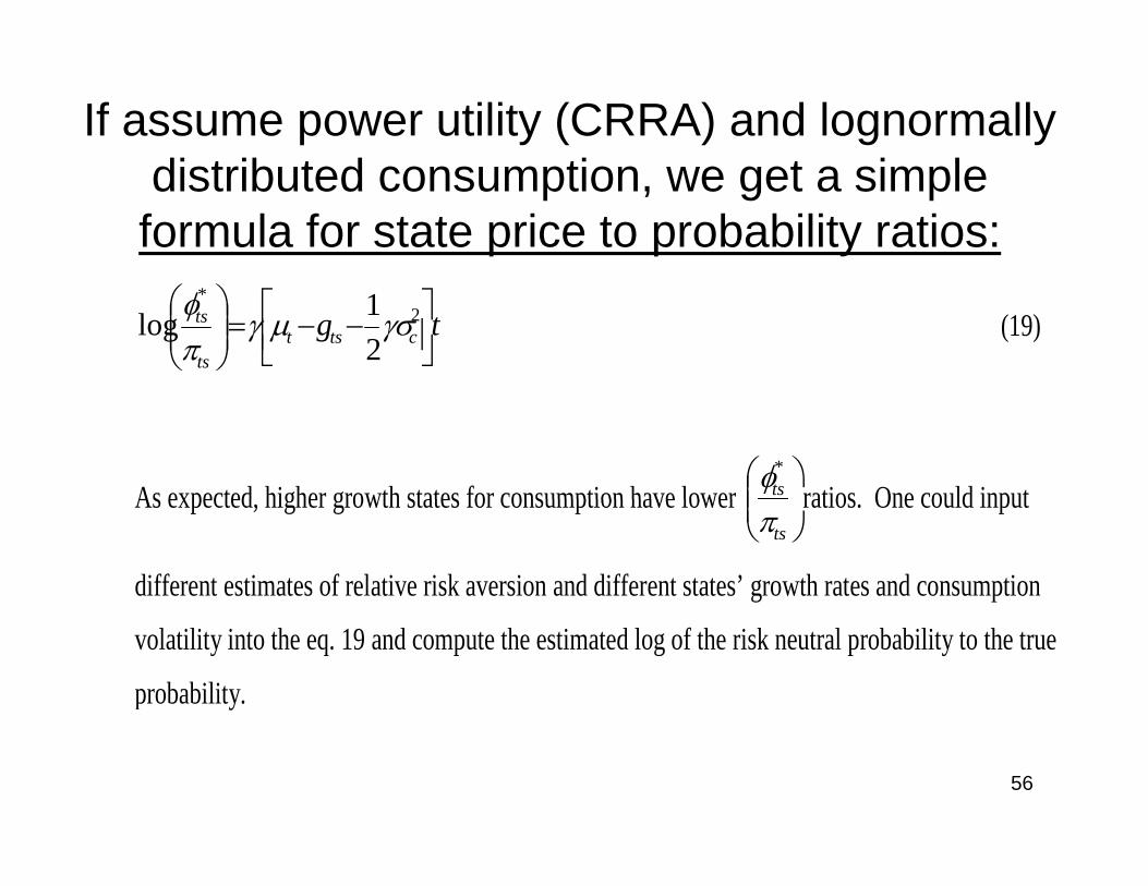
If assume power utility (CRRA) and lognormallydi t ib t d ti t i ldistributed consumption, we get a simple formula for state price to probability ratios:
tg ctstts
ts⎥⎦⎤
⎢⎣⎡ −−=⎟⎟
⎠
⎞⎜⎜⎝
⎛ 2*
21log γσμγ
πφ
(19)
As expected higher growth states for consumption have lower ⎟⎟⎞
⎜⎜⎛ tsφ
*
ratios One could inputAs expected, higher growth states for consumption have lower ⎟⎟⎠
⎜⎜⎝ tsπ
ratios. One could input
different estimates of relative risk aversion and different states’ growth rates and consumption
volatility into the eq. 19 and compute the estimated log of the risk neutral probability to the true
probability.
56

57
58

Illustration of True Probabilities Related to Risk Neutral ProbabilitiesTrue probability = K*Risk Neutral x exp(Gamma*(gts ‐ mu)) Assumes: CRRA‐Lognormal real growth modelReal Growth on Nominal Rate: 1998 to 2011 Data Real Growth on Nominal Rate: 1977 to 1997 DataIntercept 3 71 (t 2 2) Intercept 4 11 (t 3 2)Intercept ‐3.71 (t= ‐2.2) Intercept 4.11 (t= 3.2)Slope 1.42 (t= 3.8) Slope ‐0.12 (t= ‐0.8)
MuCgrow 3 MuCgrowt 3
Relative Risk Aversion (Gamma) Relative Risk Aversion (Gamma)Nominal Real 2 4 8 Nominal Real 2 4 8
Rate Growth Ratio of True Probability to Risk Neutral* Rate Growth Ratio of True Probability to Risk Neutral*1 ‐2.29 0.90 0.81 0.65 1 3.99 1.02 1.04 1.082 0 87 0 93 0 86 0 73 2 3 87 1 02 1 04 1 072 ‐0.87 0.93 0.86 0.73 2 3.87 1.02 1.04 1.073 0.55 0.95 0.91 0.82 3 3.75 1.02 1.03 1.064 1.97 0.98 0.96 0.92 4 3.63 1.01 1.03 1.055 3.39 1.01 1.02 1.03 5 3.51 1.01 1.02 1.046 4.81 1.04 1.08 1.16 6 3.39 1.01 1.02 1.036 4.81 1.04 1.08 1.16 6 3.39 1.01 1.02 1.037 6.23 1.07 1.14 1.29 7 3.27 1.01 1.01 1.028 7.65 1.10 1.20 1.45 8 3.15 1.00 1.01 1.019 9.07 1.13 1.27 1.63 9 3.03 1.00 1.00 1.0010 10.49 1.16 1.35 1.82 10 2.91 1.00 1.00 0.99
11 2.79 1.00 0.99 0.9812 2.67 0.99 0.99 0.9713 2.55 0.99 0.98 0.9614 2.43 0.99 0.98 0.9615 2 31 0 99 0 97 0 95
59
15 2.31 0.99 0.97 0.95*=Up to a scalar multiple 16 2.19 0.98 0.97 0.94