cellular neural network as a non-linear filter of impulse noise · · 2017-04-19cellular neural...

Cellular Neural Network as a Non-linear Filter of Impulse Noise

Elena Solovyeva Saint-Petersburg Electrotechnical University “LETI”

Saint-Petersburg, Russia [email protected]

Abstract—Feedforward discrete-time cellular neural network for filtering of impulse noise from two-dimensional (image) signals is represented. The parameters of mathematical filter model result from approximation problem solution in mean-square norm. It is shown that the cellular neural network surpasses median filter, Volterra filter and perceptron neural network in accuracy of image restoration and in simplicity of filter implementation.

I. INTRODUCTION One of major problems in the communication theory is

non-linear filtering of non-Gaussian noise. The impulse noise relates to non-Gaussian noise. This noise emerges during the switching of different electronic devices, in cases of mechanical damages of surfaces of the data storage devices, during the operation of internal-combustion engines, under the impact of various atmospheric phenomena, etc. Non-Gaussian noise distorts the working signals. Its emerging leads to the impairment of data transmission in communication channels [1–4].

Non-Gaussian noise is not cancelled by the methods of linear signal processing, so the methods of non-linear signal processing are used for non-Gaussian noise suppression, in particular, the methods within the framework of the “black box” principle. In view of this principle, the methods of building multidimensional polynomials and neural networks for non-linear devices, such as transformers, filters, compensators etc., are developed [5–7].

In recent years numerous non-linear filters are synthesized in the form of neural networks, which are universal approximators, and in some cases, they are simpler in comparison with multidimensional polynomials [6], [7].

The solving of an approximation problem results in establishing mapping between the input and output signals of a device and gaining high accuracy independently of computational cost (time, memory and et .)

In this paper, the cellular neural network is considered as a model of non-linear filters for cancelling non-Cassian noise (for instance, impulse noise). The synthesis of combined filters based on the cascade connection of a median filter and neural network is proposed. The mathematical model of combined filter, containing the cellular neural network, is compared with the models of combined filters, including the perceptron

network and Volterra series. The numerical results of impulse noise filtering from distorted images show the advantage of using the cellular neural network over the perceptron network and Volterra series.

The rest of the paper is summarized as follows. In Section II, the problem for impulse noise filtering is introduced. Section III presents the concept of cellular neural networks. Section IV highlights the cellular neural network difference from the commonly used neural networks and the description of image signals and impulse noise. Section IV consists of numerical results of image restoring by various non-linear filters. The conclusions are drawn in the last section.

II. THE PROBLEM OF IMPULSE NOISE FILTERING FOR IMAGE RESTORATION

The problem of synthesizing the digital impulse noise filters can be solved within the framework of the “black box” principle [2], [5], [6], when filter operator sF establishes a unique relationship between the set of input ( )s n ( ( )s n S )

and output ( )oy n ( ( )o oy n Y ) signals of device

( ) ( )osy n F s n .

For nonlinear dynamic system modeling it is required to approximate nonlinear operator sF by nonlinear operator F

which reflects the input set X on the output set oY with error , 0 , that is

)()( nxFny

where 0, nn G is the normalized discrete time, nG is the duration of input signals.

The digital filter synthesis a consists in building a mathematical model in the form of operator equation

( ) ( )y n F s n ,

where ( )y n is the output signal of the filter model, F is

operator approximating sF on sets S and oY under the condition

______________________________________________________PROCEEDING OF THE 20TH CONFERENCE OF FRUCT ASSOCIATION

ISSN 2305-7254

( ) ( )oy n y n

for all ( )s n S , ( )o oy n Y . Here is the assigned error of simulation.

The parameters of nonlinear operator F are determined by solving the approximation problem

( ) ( ) minoD

y n F s n , (1)

where D is the parameter set of operator F . In practice, the approximation error is usually estimated in the mean-square norm.

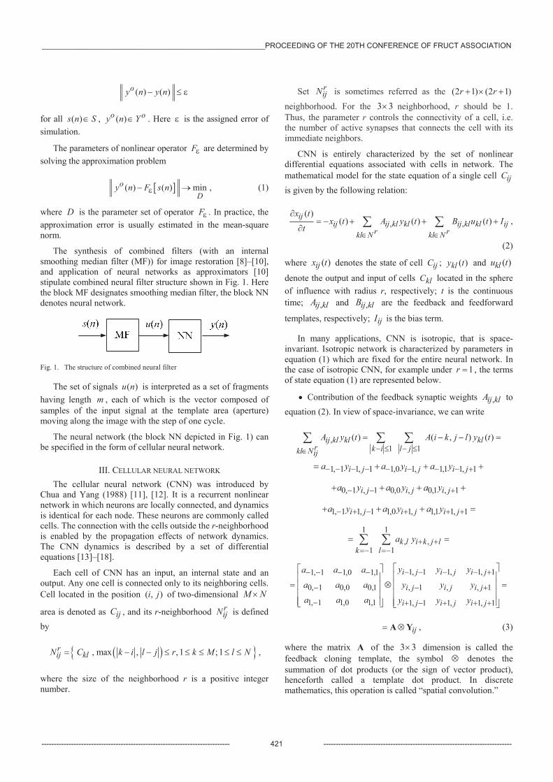
The synthesis of combined filters (with an internal smoothing median filter (MF)) for image restoration [8]–[10], and application of neural networks as approximators [10] stipulate combined neural filter structure shown in Fig. 1. Here the block MF designates smoothing median filter, the block NN denotes neural network.

Fig. 1. The structure of combined neural filter

The set of signals ( )u n is interpreted as a set of fragments having length m , each of which is the vector composed of samples of the input signal at the template area (aperture) moving along the image with the step of one cycle.

The neural network (the block NN depicted in Fig. 1) can be specified in the form of cellular neural network.

III. CELLULAR NEURAL NETWORK The cellular neural network (CNN) was introduced by

Chua and Yang (1988) [11], [12]. It is a recurrent nonlinear network in which neurons are locally connected, and dynamics is identical for each node. These neurons are commonly called cells. The connection with the cells outside the r-neighborhood is enabled by the propagation effects of network dynamics. The CNN dynamics is described by a set of differential equations [13]–[18].

Each cell of CNN has an input, an internal state and an output. Any one cell is connected only to its neighboring cells. Cell located in the position ( , )i j of two-dimensional M N

area is denoted as ijC , and its r-neighborhood rijN is defined

by

, max , ,1 ;1rij klN C k i l j r k M l N ,

where the size of the neighborhood r is a positive integer number.

Set rijN is sometimes referred as the (2 1) (2 1)r r

neighborhood. For the 3 3 neighborhood, r should be 1. Thus, the parameter r controls the connectivity of a cell, i.e. the number of active synapses that connects the cell with its immediate neighbors.

CNN is entirely characterized by the set of nonlinear differential equations associated with cells in network. The mathematical model for the state equation of a single cell ijC is given by the following relation:

, ,( )

( ) ( ) ( )ijij ij kl kl ij kl kl ij

r rkl N kl N

x tx t A y t B u t I

t,

(2)

where ( )ijx t denotes the state of cell ijC ; ( )kly t and ( )klu t

denote the output and input of cells klC located in the sphere of influence with radius r, respectively; t is the continuous time; ,ij klA and ,ij klB are the feedback and feedforward

templates, respectively; ijI is the bias term.

In many applications, CNN is isotropic, that is space-invariant. Isotropic network is characterized by parameters in equation (1) which are fixed for the entire neural network. In the case of isotropic CNN, for example under 1r , the terms of state equation (1) are represented below.

Contribution of the feedback synaptic weights ,ij klA to equation (2). In view of space-invariance, we can write

,1 1

( ) ( , ) ( )ij kl kl klr k i l jkl Nij

A y t A i k j l y t

1, 1 1, 1 1,0 1, 1,1 1, 1i j i j i ja y a y a y

0, 1 , 1 0,0 , 0,1 , 1i j i j i ja y a y a y

1, 1 1, 1 1,0 1, 1,1 1, 1i j i j i ja y a y a y 1 1

, ,1 1

k l i k j lk l

a y

1, 1 1, 1, 11, 1 1,0 1,1

0, 1 0,0 0,1 , 1 , , 1

1, 1 1,0 1,1 1, 1 1, 1, 1

i j i j i j

i j i j i j

i j i j i j

y y ya a a

a a a y y y

a a a y y y

ijA Y , (3)

where the matrix A of the 3 3 dimension is called the feedback cloning template, the symbol denotes the summation of dot products (or the sign of vector product), henceforth called a template dot product. In discrete mathematics, this operation is called “spatial convolution.”


---------------------------------------------------------------------------- 421 ----------------------------------------------------------------------------

The 3 3 matrix ijY in (2) can be obtained by moving an

opaque mask with the 3 3 window to the position ( , )i j of the M N output image Y , henceforth called the output image at ( , )C i j .

An element kla is called the center (respectively, surround) element, the weight or coef cient, of the feedback template A , if and only if ( , ) (0, 0)k l (respectively, ( , ) (0, 0)k l ).

Contribution of the input synaptic weights ,ij klB to equation (2). Following the above notes, we can write

,1 1

( ) ( , ) ( )ij kl kl klr k i l jkl Nij

B u t B i k j l u t

1 1, ,

1 1k l i k j l

k lb u

1, 1 1, 1, 11, 1 1,0 1,1

0, 1 0,0 0,1 , 1 , , 1

1, 1 1,0 1,1 1, 1 1, 1, 1

i j i j i j

i j i j i j

i j i j i j

u u ub b b

b b b u u u

b b b u u u

ijB U , (4)

where the 3 3 matrix B is called the feedforward or input cloning template, and ijU is the translated masked input image.

Contribution of the threshold term to equation (2). In view of space-invariance, denote ijI z .

Using the above notations in (3), (4), space-invariant CNN is completely described by state equation

ij ij ij ijx x zA Y B U . (5)

The output signal of cell ijC is given by the following equation

( ) ( ( ))ij ijy t f x t , (6)

where ( )ijy t denotes the output value of cell ijC , ( )f is the non-linear activation function which is usually specified as the unity gain piecewise linear saturation function described by expression

1( ) ( ( )) ( ) 1 ( ) 12ij ij ij ijy t f x t x t x t

and shown in Fig. 2.

The properties of the piecewise linear saturation function shown in Fig. 2 are the following:

an uniform gain for low and high input signal amplitudes,

quickness of signal conversion,

implementation simplicity in the analog and digital fields using operational amplifiers and VLSI technology respectively.

)(txij

)(tyij

Fig. 2. The piecewise linear saturation function

A signi cant CNN feature is that CNN has two independent input capabilities: the generic input and the initial state of cells. They are normally bounded by ( ) 1iju t and

(0) 1ijx . Similarly, if ( ) 1f then ( ) 1ijy t .

CNN is uniquely de ned by three terms of the cloning templates , , zA B , which consist of 19 real numbers for the 3 3 neighborhood ( 1r ).

One of the simplest CNN subclasses is zero-feedback (feedforward) CNN. CNN belongs to the zero-feedback subclass if and only if all the feedback template elements are zero, i.e., 0A . In view of (5) each cell of the zero-feedback CNN is described by expression

ij ij ijx x zB U . (7)

The discrete CNN model is used for image processing. The feedforward CNN description in discrete time domain results from expression (7) after following transformations:

– the approximation of derivative

( ) ( ) ( )( ) ( 1)ij ij ij

ij ijdx t x t x t t

x n x ndt t

where n is the discrete normalized time. Let us suppose, that 1t ;

– the transition from differential equation (6) to recursive difference equation

( ) ( 1) ( 1)ij ij i ijjx n x n x n zB U .

Eventually, on the bases of (6) and (7) the model of cell ijC in feedforward discrete-time CNN (DTCNN) is described

as

( ) jij ix n zB U ,


---------------------------------------------------------------------------- 422 ----------------------------------------------------------------------------

( ) ( )ij ijy n f x n . (8)

The structure of cell ijC in feedforward DTCNN is depicted in Fig. 3.

( 1)klu n

( )ijx n ( )ijy n

rijkl N

Fig. 3. The structure of cell ijC in feedforward DTCNN

Expressions (8) are transformed into the isotropic model of DTCNN cell if the parameters of model are fixed for entire neural network.

IV. THE SIGNALS OF IMAGES AND THE CRITERION OF FILTRATION ACCURACY ESTIMATION

Combined neural filters are synthesized on the class of bit-map (dot element) half-tone images at the resolution measured by 256 gray levels, i.e., image is the matrix of integers (elements of brightness, pixels) in the interval [0; 255]. In the case under consideration, the pixel format is unit8.

The impulse noise represents switched on and switched off pixels (white and black dots in the picture), the emergence of which does not depend on the presence of noise spikes in adjacent dots. The addition of impulse interference to image implies that value q of the signal sample with probability aP is replaced with value 0z (black), with probability bP is replaced with value 255z (white), and with probability 1 ( )a bP P remains unchanged. Thus, the probability

density of the impulse noise is described by the following expression

at 0;( ) at 255;

0 in other cases

a

b

P qp q P q

or

( ) ( ) ( )a bp q P q a P q b ,

where ( ) is the -function. Let us assume that a bP P . The impulse noise model described above is referred to as “salt and pepper” [4], [9], [10].

In building operator F of nonlinear filter, the “unit8”

format of signals ( )u n U and ( )o oy n Y is transformed into the “double” format (samples of signals are normalized floating-point numbers of double precision in the range

1;1 ).

The synthesis of combined neural filter (Fig. 1) with internal isotropic feedforward DTCNN, including some neurons in hidden layer and referred to as combined DTCNN (CDTCNN), is performed in the MATLAB system environment. This synthesis involves solving the approximation problem (1) in the mean-square norm using the error back propagation algorithm [6]. Activation function f is specified in the form of piecewise linear saturation one (Fig. 2). The distorted image “Tigers” having the size of 220 148 pixels is a learning signal.

The results of CDTCNN filtration are compared with the results of combined neural filtration (Fig. 1) with internal two-layer perceptron network (TLPN), including the hyperbolic tangent activation functions, referred to as combined TLPN (CTLPN) [10], of combined Volterra filtration [5], [6] and of median filtration performed at the 3x3 square aperture [4].

The TLPN model is described by equation

01 0

( ) ( )I m

d dg gd g

y n G c c G w u n ,

where model input signal is the vector

0 1 2, , , ..., mu n u n u n u n ,

containing 0 ( ) 1u n , as well as elements, corresponding matrix ijU in (4), from the 3 3 window located around cell

( , )C i j ; 9m ; G is the hyperbolic tangent activation function; I is the number of neurons.

The structure of two-layer perceptron network is shown in Fig. 4.

mu n

)(ny

0u n

1u n

10w

20w

0Iw

1Iw

Imw

21w

mw2

11wmw1

1c

2c

Ic

0c

Fig. 4. The structure of two-layer perceptron network


---------------------------------------------------------------------------- 423 ----------------------------------------------------------------------------

Combined Volterra filter (CVF) is the cascade connection of two units: MF with the 3x3 square aperture and Volterra filter. The CVF structure has the similar form depicted in Fig. 1, but the block NN is replaced with Volterra filter. The CVF model is the truncated Volterra series [5], [6]:

1 1 11 2

1 0 0 0 11 2 ... , , ...,

L J J Jr

j j j ry n h j j j u n j ,

(9) where 1 2, , ... , h j j j is the Volterra kernel of order , ( 1)J is the CVF memory length, L is the degree of Volterra model. The set of signals ( )u n U is formed at the output of smoothing MF and consists of J-length fragments, each of which is built at the aperture moving along the picture with a step of one cycle.

Parameters of the VCF model (9) are defined as a result of solving the approximation problem (1) in the mean-square norm while using learning image with the size of 220 148 pixels. The length of learning sequence ( )u n amounts to 32560 samples.

CDTCNN and CTLPN comprise different activation functions. The properties of the piecewise linear saturation function shown in Fig. 2 are considered above.

The properties of the hyperbolic tangent activation function, which is shown in Fig. 5 and contained in CTLPN, are the following:

– gain control for the input signals of different levels. The central function part corresponding to the region of low input signal amplitudes has a large slope and a maximum of the derivative, so the gain is maximum here. Moving from the function central to large absolute values of inputs, the slope of the curve and its derivative is decreased, as well as the gain is reduced;

the function is continuous and differentiable over the entire range of argument, that is convenient on using this function in the gradient algorithms of learning network when multiple operations of differentiation are required; the slow conversion of signal; more complicated implementation of the hyperbolic tangent activation function as compared with the piecewise linear function.

1

1

0

( ( ))G x n

( )x n

Fig. 5. The hyperbolic tangent activation function

The rate of impulse noise suppression by different filters is estimated with the help of error computed after the restoration of a test image having the size of 220 148 pixels by the following formula

2

1

1 ( ) ( )Q

o

ny n y n

Q, (10)

where ( )y n is the output signal of non-linear filter, ( )oy n is desirable signal, 32 560Q . The test images differ from learning one.

V. IMPULSE NOISE CANCELLING BY NON-LINEAR FILTERS The filtration results (error calculated from (10)) obtained

by synthesized devices are summarized in the Table I, the Table II, Fig. 6 and Fig. 7 under various densities p of the impulse noise. “Tigers”, “Building” and “Fence” are the names of learning and two test images, correspondently. All the images have the size of 220 148 pixels.

Neural filters built on the base of CDTCNN and CTLPN comprise two and five neurons in hidden layer under the impulse noise density 0.3p and 0.5p correspondingly. The filtration errors are decreased very slowly at neuron numbers higher than mentioned ones.

CVF model is applied in the form of Volterra polynomial (9) of the second degree.

The number of parameters in neural and polynomial models is indicated in the Table III.

TABLE I. FILTRATION ERROR UNDER P=0.3

Image CDTCNN CTLPN CVF MF

Tigers 514 516 534 739

Building 786 804 835 1039

Fence 1142 1138 1153 1434

TABLE II. FILTRATION ERROR UNDER P=0.5

Image CDTCNN CTLPN CVF MF

Tigers 771 841 1206 2759

Building 1083 1186 1712 3014

Fence 1558 1800 2214 3735

TABLE III. NUMBER OF MODEL PARAMETERS

Model Impulse noise density 0.3 0.5

CDTCNN 23 56

CVF 54 54

The following inferences can be made from the Table I, the Table II and Fig. 6.

At the middle noise density ( 0.3p ), CDTCNN and CTLPN comprise two neurons in hidden layer and 23 parameters. These filters ensure virtually identical accuracy of filtration. Thus, differences in the activation functions of these filters are not revealed in the case of low neuron number.


---------------------------------------------------------------------------- 424 ----------------------------------------------------------------------------

a b

c d

e f

Fig. 6. Learning image and filtration results: a – initial image, b – distorted image, c – CDTCNN result, d – CTLPN result, e – CVF result, f – MF result

CDTCNN and CTLPN yield higher quality of image restoration (Fig. 6, c, d) than CVF model of the second degree (Fig. 6, e) and MF (Fig. 6, f).

a b

c d

e f

Fig. 7. Test image and filtration results: a – initial image, b – distorted image, c – CDTCNN result, d – CTLPN result, e – CVF result, f – MF result

In practice, CDTCNN is more preferable in comparison with CTLPN since its hardware implementation is simple due to using the piecewise linear saturation functions.


---------------------------------------------------------------------------- 425 ----------------------------------------------------------------------------

From the Table II, the Table III and Fig. 7, it should be added the following notes.

At the high noise density ( 0.5p ), when CDTCNN and CTLPN contain five neurons in hidden layer, CDTCNN with the piecewise linear activation function yields higher filtration precision (Fig. 7, c), than CTLPN with the hyperbolic tangent activation functions (Fig. 7, d), CVF model of the second degree (Fig. 7, e) and MF (Fig. 7, f).

It should be observed that CDTCNN, CTLPN and CVF provide different accuracy at the nearly equal complexity of these filters (56 parameters of CDTCNN and CTLPN, 54 parameters of CVF).

The use of the hyperbolic tangent activation functions in CTLPN negatively affects the image quality (white color turns to gray one, as well as there is a bit ripple i.e. image loses its smoothness (Fig. 7, d)).

Indeed, at an equal probability of the impulse noise (for instance, white and black dots on images) occurrence, the filtration with different gains at low and high amplitudes of signals (in the case of the hyperbolic tangent and the logistic activation function) is not expedient.

VI. CONCLUSION The problem of non-Gaussian noise filter synthesis is often

effectively solved within the framework of the "black box" principle. According to this principle, the mathematical filter model describes the relationship between the sets of input and output signals. The model parameters are determined by solving the approximation problem using the subsets of input and output signals. Considered approach to the synthesis of nonlinear filters is general, because it can be applied at various kinds of non-Gaussian noise sources.

Neural filters such as a feedforward cellular neural network and a two-layer perceptron network surpass Volterra filter and median filter in the accuracy of impulse noise filtration on half-tone images. The above-mentioned neural filters yield equal accuracy at the middle noise density. The feedforward cellular neural network in the standard version (with the piecewise linear saturation functions) carries out more accurate restoration of images as compared with two-layer perceptron network (with the hyperbolic tangent or the logistic activation function) at the high noise density.

It should be emphasized that the hardware implementation of the cellular neural network is simpler in comparison with two-layer perceptron network since the piecewise linear saturation functions used in the cellular network are simpler than the hyperbolic tangent activation functions included in perceptron network.

ACKNOWLEDGMENT This work was supported by Saint Petersburg

Electrotechnical University “LETI” according to the base part of the state scientific work from the Russian Education Ministry.

REFERENCES [1] S.V. Vaseghi, Advanced digital signal processing and noise

reduction. New York: John Wiley & Sons, Ltd, 2008. [2] I. Pitas and A. N. Venetsanopoulos, Nonlinear digital filters:

principles and applications. Kluver Academic Publishers, 1990.

[3] S. Haykin, Digital communication systems. New York: John Wiley & Sons Inc., 2013.

[4] R.C. Gonzalez and R.E. Woods, Digital image processing. Higher Education, 2008.

[5] V.J. Mathews and G.L. Sicuranza, Polynomial signal processing. New York: John Wiley & Sons, Inc., 2000.

[6] A. Janczak, Identification of nonlinear systems using neural networks and polynomial models. A Block-Oriented Approach. Springer-Verlag Berlin Heidelberg, 2005.

[7] Speech, audio, image and biomedical signal processing using neural networks / Editors: Bhanu Prasad, S.R. Mahadeva Prasanna. Springer-Verlag Berlin Heidelberg, 2008.

[8] A.A. Lanne and E.B. Solovyeva, “Nonlinear filtration of images with pulse interferences (theoretical principles)”, Radioelectronics and Communications Systems, vol.43, no. 3, 2000, pp. 546-553.

[9] A.A. Lanne and E.B. Solovyeva, “Nonlinear filtration of images with pulse interferences (examples of realization)”, Radioelectronics and Communications Systems, vol.43, no. 4, 2000, pp. 546-553.

[10] E.B. Solovyeva and S.A. Degtyarev, “Synthesis of neural pulse interference filters for image restoration”, Radioelectronics and Communications Systems, vol. 51, no. 12, 2008, pp. 661-668.

[11] L.O. Chua and L. Yang, “Cellular neural networks: Theory”. IEEETransactions on Circuits and Systems, vol. 35, no. 10, 1988, pp. 1257-1272.

[12] L.O. Chua and L. Yang, “Cellular neural networks: Applications”. IEEE Transactions on Circuits and Systems, vol. 35, no. 10, 1988, pp. 1273-1290.

[13] Chaos, CNN, Memristors and Beyond. A Festschrift for Leon Chua / Edited by: A. Adamatzky , G. Chen. Singapur: World Scientific Publishing Co. Pte. Ltd., 2013.

[14] L.O. Chua and T. Roska, Cellular Neural Networks and Visual Computing: foundations and applications. Cambridge: Cambridge Univ. Press, 2002.

[15] M.E. Yalcin, J.A.K Suykens, and J.P.L. Vandewalle, Cellular Neural Networks, Multi-Scroll Chaos And Synchronization. World Scientific Publishing Co. Pte. Ltd., 2005.

[16] J. Kung, D. Kim, and S. Mukhopadhyay, “On the impact of energy-accuracy tradeoff in a digital cellular neural network for image processing”, IEEE Transactions on Computer-Aided Design of Integrated Circuits and Systems, vol. 34, no. 7, 2015, pp. 1070-1081.

[17] S. Duan, X. Hu, Z. Dong, L. Wang, and P. Mazumder, “Memristor-based cellular nonlinear/neural network: design, analysis, and applications”, IEEE Transactions on Neural Networks and Learning Systems, vol. 26, no. 6, 2015, pp. 1202-1213.

[18] J. Muller, Jan Muller, R. Braunschweig, and R. Tetzlaff, “A cellular network architecture with polynomial weight functions”, IEEETransactions on Very Large Scale Integration (VLSI) Systems, vol. 24, no. 1, 2016, pp. 353-357.


---------------------------------------------------------------------------- 426 ----------------------------------------------------------------------------

cellular neural network as a non-linear filter of impulse noise · · 2017-04-19cellular neural...

Documents