Chapter 7Chapter 7 Finite Impulse Response(FIR) Finite Impulse Response(FIR)

Filter DesignFilter Design

2/74

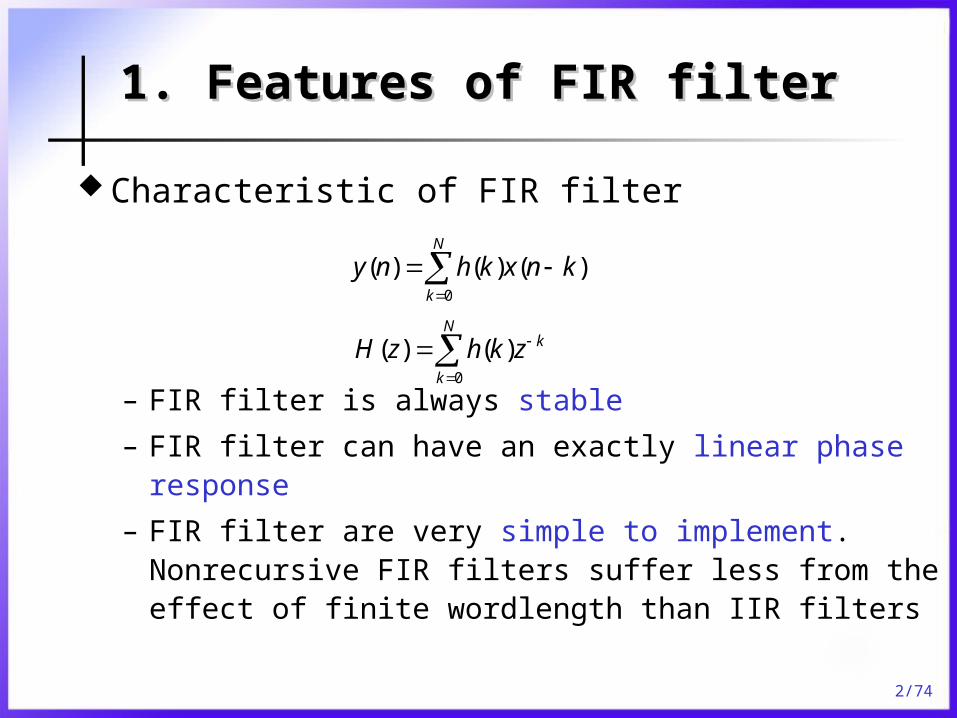
Characteristic of FIR filter

– FIR filter is always stable

– FIR filter can have an exactly linear phase response

– FIR filter are very simple to implement. Nonrecursive FIR filters suffer less from the effect of finite wordlength than IIR filters

1. Features of FIR filter1. Features of FIR filter

0

( ) ( ) ( )N

k

y n h k x n k

0

( ) ( )N

k

k

H z h k z

3/74

Phase response of FIR filter

– Phase delay and group delay

2. Linear phase response2. Linear phase response

0

( )

( ) ( )

= ( )

Nj T j kT

k

j T j

H e h k e

H e e

where ( ) arg ( )j TH e

p g( )

p

( )g

d

d

(1)

(2)

4/74

– Condition of linear phase response

( )

( )

Where and is constant Constant group delay and phase delay response

(3)

(4)

5/74

• If a filter satisfies the condition given in equation (3)

– From equation (1) and (2)

1 0

0

( )

( )sin = tan

( )cos

N

nN

n

h n nT

h n nT

thus

0

0

( )sintan =

( ) cos

N

nN

n

h n nT

h n nT

6/74

– It is represented in Fig 7.1 (a),(b)

0

( ) cos sin sin cos 0N

n

h n nT nT

0

( )sin( ) 0N

n

h n nT

( ) ( 1), 0h n h N n n N

/ 2NT

7/74

• When the condition given in equation (4) only

– The filter will have a constant group delay only

– It is represented in Fig 7.1 (c),(d)

( ) ( )h n h N n

/ 2NT

/ 2

8/74

Center of symmetry

Fig. 7-1.

9/74

Table 7.1 A summary of the key point about the four types of linear phase FIR filters

10/74

Example 7-1(1) Symmetric impulse response for linear phase response.

No phase distortion

(2)

( ) ( ) or ( ) ( )h n h N n h n h N n

( ) ( ), 0 , 10h n h N n n N N

(0) (10)

(1) (9)

(2) (8)

(3) (7)

(4) (6)

h h

h h

h h

h h

h h

11/74

• Frequency response ( )H

10

0

2 3 4 5

6 7 8 9 10

5

( ) ( )

= ( )

= (0) (1) (2) (3) (4) (5)

+ (6) (7) (8) (9) (10)

= [ (0)

j T

jk T

k

j T j T j T j T j T

j T j T j T j T j T

j T

H H e

h k e

h h e h e h e h e h e

h e h e h e h e h e

e h

5 4 3 2

2 3 4 5

(1) (2) (3) (4) (5)

+ (6) (7) (8) (9) (10) ]

j T j T j T j T j T

j T j T j T j T j T

e h e h e h e h e h

h e h e h e h e h e

5 5 5 4 4 3 3

2 2

5

( )= [ (0)( ) (1)( ) (2)( )

(3)( ) (4)( ) (5)]

[2 (0)cos(5 ) 2 (1)cos(4 ) 2 (2)cos(3 )

2 (3)c

j T j T j T j T j T j T j T

j T j T j T j T

j T

H e h e e h e e h e e

h e e h e e h

e h T h T h T

h

os(2 ) 2 (4)cos( ) (5)]T h T h 5

5 ( )

0

( )= ( )cos( ) ( )j T j

k

H a k k T e H e

where 5

0

( ) = ( )cos( )k

H a k k T

( ) 5 T

12/74

(3) 9N (0) (9)

(1) (8)

(2) (7)

(3) (6)

(4) (5)

h h

h h

h h

h h

h h

9 /2 9 9 7 7 5 3

3 3

9 /2

( )= [ (0)( ) (1)( ) (2)( )

(3)( ) (4)( )]

[2 (0)cos(9 / 2) 2 (1)cos(7 / 2) 2 (2)cos(5 / 2)

2

j T j T j T j T j T j T j T

j T j T j T j T

j T

H e h e e h e e h e e

h e e h e e

e h T h T h T

( )

(3)cos(3 / 2) 2 (4)cos( / 2)]

= ( ) j

h T h T

H e

5

1

( )= ( )cos[ ( 1/ 2) ]k

H b k k T

where

( ) (9 / 2) T 1 1

( ) 2 ( ), 1, 2, ,2 2

N Nb k h k k

13/74

Transfer function for FIR filter

3. Zero distribution of FIR filters3. Zero distribution of FIR filters

0

( ) ( )N

k

k

H z h k z

0

0

1

( ) ( )

= ( )

= ( )

Nk

k

k N

k N

N

H z h N k z

h k z z

z H z

14/74

Four types of linear phase FIR filters– have zero at ( )H z 0z z

0jz re

1 10

jz r e

is real and is imaginary( )h n 0z*

0jz re

* 1 10( ) jz r e

1 1 1 1 1 1(1 )(1 )(1 )(1 )j j j jre z re z r e z r e z

15/74

– If zero on unit circle

– If zero not exist on the unit circle

– If zeros on

1, 1/ 1r r

0jz e

1 *0 0

jz e z

1 1(1 )(1 )j je z e z

1 1 1(1 )(1 )rz r z

1z 1(1 )z

16/74

Necessary zero

Necessary zero

Necessary zero

Necessary zero

Fig. 7-2.

17/74

Filter specifications

4. FIR filter specifications4. FIR filter specifications

peak passband deviation (or ripples)

stopband deviation

passband edge frequency

stopband edge frequency

sampling frequency

p

r

p

r

s

18/74

ILPF

Satisfies spec’s

Fig. 7-3.

19/74

Characterization of FIR filter

– Most commonly methods for obtaining • Window, optimal and frequency sampling methods

0

( ) ( ) ( )N

k

y n h k x n k

0

( ) ( )N

k

k

H z h k z

( )h k

20/74

FIR filter– Frequency response of filter

– Corresponding impulse response

– Ideal lowpass response

5. Window method5. Window method

( )IH

( )Ih n

1( ) ( )

2j n

I Ih n H e d

1 1( ) 1

2 22 sin( )

, 0, - =

2 , 0

c

c

j n j nI

c c

c

c

h n e d e d

f nn n

n

f n

21/74

Fig. 7-4.

22/74

Truncation to FIR

– Rectangular Window

( ) ( ) ( ) "windowing"Ih n h n w n

12

( )12

) ) )

) )

j j jI

j jI

H(e H (e W(e

H (e W(e d

1 , 0,1,...,( )

0 ,

n Nw n

elsewhere

23/74

Fig. 7-5.

24/74

Fig. 7-6.

25/74

Fig. 7-7.

26/74

Table 7.2 summary of ideal impulse responses for standard frequency selective filters

and are the normalized passband or stopband edge frequencies; N is the length of filter

1, cf f2 f

( )Ih n

( )Ih n

( )Ih n

27/74

Common window function types– Hamming window

0.54 0.46cos 2 / , 0

0 ,

n N n Nw n

elsewhere

3.32 /F N

where N is filter length and

is normalized transition widthF

28/74

– Characteristics of common window functions

Fig. 7-8.

29/74

Table 7.3 summary of important features of common window functions

30/74

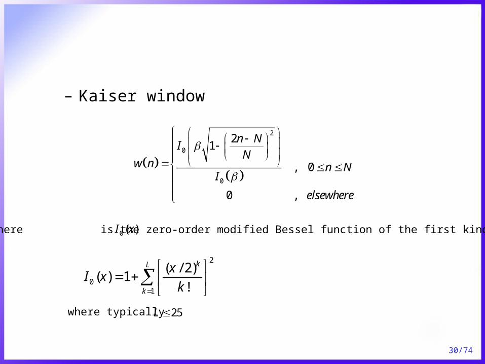
– Kaiser window

2

0

0

21

, 0

0 ,

n NI

Nw n n N

I

elsewhere

2

01

( / 2)( ) 1

!

kL

k

xI x

k

where typically

where is the zero-order modified Bessel function of the first kind0 ( )I x

25L

31/74

• Kaiser Formulas – for LPF design

10

0.4

20log ( )

min( , )

0, if 21dB

0.5842( 21) 0.07886( 21), if 21dB 50dB

0.1102( 8.7) if

p s

A

A

A A A

A A

50dB

7.95

14.36

AN

F

32/74

Example 7-2– Obtain coefficients of FIR lowpass using hamming

window

• Lowpass filter

Passband cutoff frequency

Transition width

Stopband attenuation

Sampling frequency

: 1.5pf kHz

: 0.5f kHz

: 8sf kHz

50dB

sin

2 , 0

2 , 0

cc

I c

c

nf n

h n n

f n

/ 0.5 / 8 0.0625sF f f

3.32 / 3.32 / 0.0625 53.12N F

54N

33/74

• Using Hamming window

( ) ( ) ( )Ih n h n w n 0 54n

( ) 0.54 0.46cos(2 / 54)w n n 0 54n ' / 2 (1.5 0.25) 1.75[ ]c pf f f kHz

' / 1.75 / 8 0.21875c c sf f f

2 sin ( )2

, , 02( ) ( )

2

2 ,2

c c

I c

c

Nf n

Nn n N

Nh n n

Nf n

34/74

2 0.218750 : (0) sin( 27 2 0.21875)

27 2 0.218750.00655

(0) 0.54 0.46cos(0) 0.08

(0) (0) (0) 0.00052398

I

I

n h

w

h h w

2 0.218751 : (1) sin( 26 2 0.21875)

26 2 0.218750.011311

(1) 0.54 0.46cos(2 / 54)

0.08311

(1) (1) (1) 0.00094054

I

I

n h

w

h h w

35/74

2 0.218752 : (2) sin( 25 2 0.21875)

25 2 0.218750.00248397

(2) 0.54 0.46cos(2 2 / 54)

0.092399

(2) (2) (2) 0.000229516

2 0.2187526 : (26) sin( 1 2 0.21875)

1 2 0.218750.312936

I

I

I

n h

w

h h w

n h

36/74

(26) 0.54 0.46cos(2 26 / 54)

0.9968896

(26) (26) (26) 0.3112226I

w

h h w

27 : (27) 2 2 0.21875

0.4375

(27) 0.54 0.46cos(2 27 / 54)

1

(27) (27) (27) 0.4375

I c

I

n h f

w

h h w

37/74

Fig. 7-9.

38/74

Example 7-3– Obtain coefficients using Kaiser or Blackman window

Passband cutoff frequency

Transition region

Sampling frequency

: 1200pf Hz

: 500f Hz

: 10sf kHz

Stopband attenuation : 40dB

passband attenuation : 0.01dB

20log(1 ) 0.01 , 0.00115p pdB

20log( ) 40 , 0.01r rdB

0.00115r p

39/74

• Using Kaiser window

7.95 58.8 7.9570.82

14.36 14.36(500 /10000)

AN

F

71N

0.1102(58.8 8.7) 5.52 ' / 1, 450 /10,000 0.145c c sf f f

2 sin2

( ) , 0

2

c c

I

c

Nf n

h n n NN

n

40/74

( ) ( ) ( )Ih n h n w n

2 0.1450 : (0) sin( 35.5 2 0.145)

35.5 2 0.145

0.00717

In h

2

0

0

0 0

21

(0)(0) 0.023

( ) (5.52)

n NI

N Iw

I I

(0) (0) (0) 0.000164935Ih h w

41/74

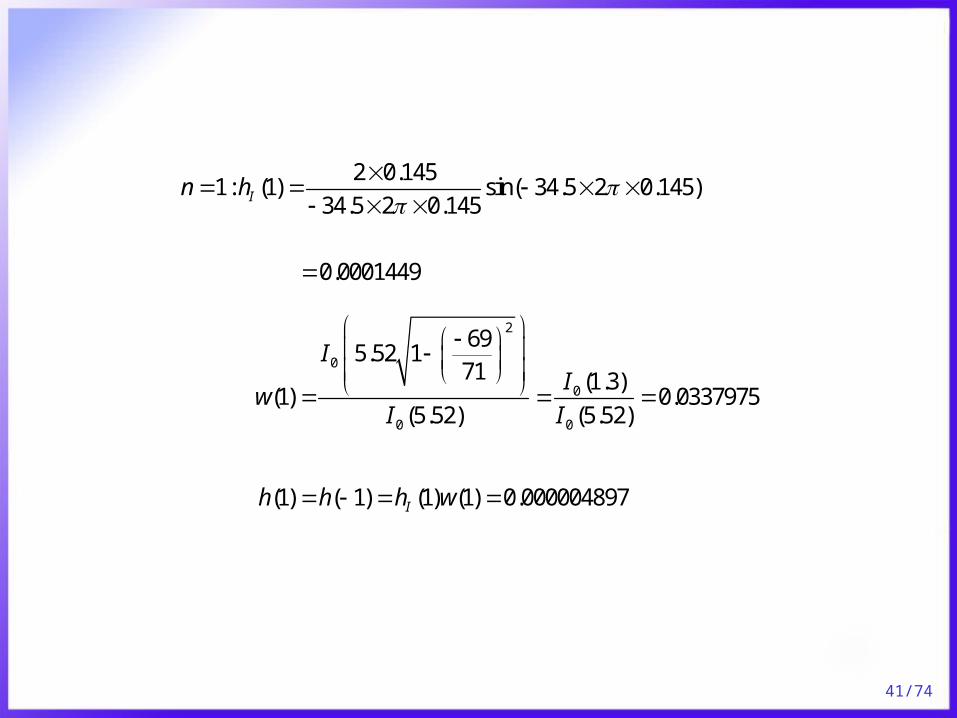
2 0.1451: (1) sin( 34.5 2 0.145)

34.5 2 0.145

0.0001449

In h

2

0

0

0 0

695.52 1

71 (1.3)(1) 0.0337975

(5.52) (5.52)

II

wI I

(1) ( 1) (1) (1) 0.000004897Ih h h w

42/74

2 0.1452 : (2) sin( 34.5 2 0.145)

33.5 2 0.145

0.007415484

In h

2

0

0

0 0

695.52 1

71 (1.8266)(2) 0.04657999

(5.52) (5.52)

II

wI I

(2) ( 2) (2) (2) 0.000345413Ih h h w

43/74

2 0.14535 : (35) sin( 0.5 2 0.145)

0.5 2 0.145

0.280073974

In h

2

0

0

0 0

15.52 1

71 (5.51945)(35) 0.999503146

(5.52) (5.52)

II

wI I

(35) ( 35) (35) (35) 0.279934818Ih h h w

44/74

Fig. 7-10.

45/74

Summary of window method1. Specify the ‘ideal’ or desired frequency response of filter,

2. Obtain the impulse response, , of the desired filter by

evaluating the inverse Fourier transform

3. Select a window function that satisfies the passband or

attenuation specifications and then determine the number of filter coefficients

4. Obtain values of for the chosen window function and the values of the actual FIR coefficients, , by multiplying

by

( )IH

( )Ih n

( )h n

( )w n

( )w n

( )Ih n( ) ( ) ( )Ih n h n w n

46/74

Advantages and disadvantages– Simplicity

– Lack of flexibility

– The passband and stopband edge frequencies cannot be precisely specified

– For a given window(except the Kaiser), the maximum ripple amplitude in filter response is fixed regardless of how large we make N

47/74

Basic concepts– Equiripple passband and stopband

• For linear phase lowpass filters– m+1 or m+2 extrema(minima and maxima)

6. The optimal method6. The optimal method

( ) ( )[ ( ) ( )]IE W H H

min[max ( ) ]E

where m=(N+1)/2 (for type1 filters) or m =N/2 (for type2 filters)

Weighted

Approx. error

Weighting

functionIdeal desired

response

Practical

response

48/74

Ideal response

Practical response

Fig. 7-11.

49/74

Fig. 7-12.

50/74

– Optimal method involves the following steps• Use the Remez exchange algorithm to find the optimum set of

extremal frequencies

• Determine the frequency response using the extremal frequencies

• Obtain the impulse response coefficients

51/74

Optimal FIR filer design

0

( ) ( )N

k

k

H z h k z

where ( ) ( )h n h n

/2 /2

1 0

( ) (0) 2 ( )cos ( )cosN N

k k

H h h k k T a k k T

where and , (0) (0)a h ( ) 2 ( )a k h k 1,2, , / 2k N

Let / 2 / 2sf f T

1

1 , 0

0 , 0.5p

r

f fH f

f f

1

, 0

1 , 0.5

p

r

f fW f k

f f

This weighting function permits different peak error in the two band

52/74

/22

0

( ) ( ) ( ) cos 2N

j f

k

H f H e a k k f

min[max ( ) ]E f

Find ( )a k

( ) ( )[ ( ) ( )]IE f W f H f H f

where are and 0, pf f ,0.5rf

53/74

– Alternation theorem

0, ,0.5p rF f f Let

If has equiripple inside bands and more than m+2 extremal point ( )E f F

then

1( ) ( ) , 0,1, , 1i iE f E f e i l

0 1 ( 1)lf f f l m

,0.50, &max ( )

p rf f fe E f

where

( ) ( )IH f H f

54/74

• From equation (7-33) and (7-34)

• Equation (7-35) is substituted equation (7-32)

• Matrix form

( ) ( ) ( ) ( 1) , 0,1,2, , 1ii i I iW f H f H f e i m

0

( ) cos 2 ( ) ( 1) , 0,1,2, , 1( )

mi

i I ik i

ea k kf H f i m

W f

0 0 0 0 0

1 1 1 1

!1 1 1 1

1 cos 2 cos 4 cos 2 1/ ( ) ((0)

1 cos 2 cos 4 cos 2 1/ ( ) (1)

1 cos 2 cos 4 cos 2 ( 1) / ( ) ( )

1 cos 2 cos 4 cos 2 ( 1) / ( )

I

mm m m m

mm m m m

f f mf W f H fa

f f mf W f a

f f mf W f a m

f f mf W f e

1

1

)

( )

( )

( )

I

I m

I m

H f

H f

H f

55/74

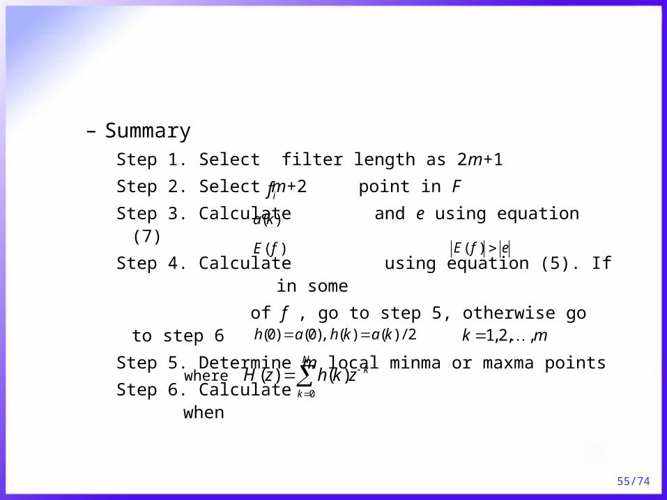
– SummaryStep 1. Select filter length as 2m+1

Step 2. Select m+2 point in F

Step 3. Calculate and e using equation (7)

Step 4. Calculate using equation (5). If in some

of f , go to step 5, otherwise go to step 6

Step 5. Determine m local minma or maxma points

Step 6. Calculate when

if

( )a k

( )E f ( )E f e

(0) (0), ( ) ( ) / 2h a h k a k 1,2, ,k m

where 0

( ) ( )N

k

k

H z h k z

56/74

– Example 7-4• Specification of desired filter

– Ideal low pass filter

– Filter length : 3

–

–

• Normalized frequency

1[rad],pT 1.2[rad]rT

2k

0 1 20.5 / 2 , 1/ 2 , 1.2 / 2f f f

57/74

• From

• Cutoff frequency

1 0.8776 2 (0) 1

1 0.5403 2 (1) 1

1 0.3624 1 0

a

a

e

0 1 2 0 1( ) ( ) 1, ( ) 0, ( ) ( ) 1/ 2I I IH f H f H f W f W f 2and ( ) 1W f

( ) 0.645 2.32cos 2H f f : not the optimal filter

0 1 2

1 1.20.5

2 2f f f

0 1 2 0( ) 1, ( ) ( ) 0, ( ) 0.5,I I IH f H f H f W f 1 2and ( ) ( ) 1W f W f

(0) 0.645, (1) 2.32,a a 0.196e

58/74

1 0.5403 2 (0) 1

1 0.3624 1 (1) 0

1 1 1 0

a

a

e

(0) 0.144, (1) 0.45,a a 0.306e

( ) 0.144 0.45cos 2H f f : has the minimum

(N=3)

max ( )E f

59/74

Fig. 7-13.

60/74

Optimization using MATLAB– Park-McClellan

– Remez

remez( )b N,F, M

remez( )b N,F, M, WT

where N is the filter order (N+1 is the filter length)

F is the normalized frequency of border of pass band

M is the magnitude of frequency response

WT is the weight between ripples

61/74

– Example 7-5• Specification of desired filter

– Band pass region : 0 – 1000Hz

– Transition region : 500Hz

– Filter length : 45

– Sampling frequency : 10,000Hz

• Normalized frequency of border of passband

• Magnitude of frequency response

[0, 0.2, 0.3, 1]F

[11 0 0]M

62/74

Table 7-4.

63/74

Fig.7-14.

64/74

– Example 7-6• Specification of desired filter

– Band pass region : 3kHz – 4kHz

– Transition region : 500Hz

– Pass band ripple : 1dB

– Rejection region : 25dB

– Sampling frequency : 20kHz

• Frequency of border of passband

[2500, 3000, 4000, 4500]F

[0 1 0]M

65/74

• Transform dB to normal value

• Filter length

– Remezord (MATLAB command)

20

20

10 1

10 1

p

p

A

p A

2010

rA

r

where and ripple value(dB) of pass band and rejection band

pA

rA

66/74

Table 7-5.

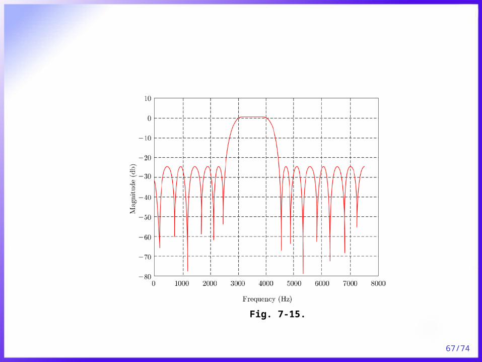
67/74

Fig. 7-15.

68/74

Frequency sampling filters– Taking N samples of the frequency response at intervals

of

– Filter coefficients

7. Frequency sampling method7. Frequency sampling method

/skF N 0,1, , 1k N

( )h n

1(2 / )

0

1( ) ( )

Nj N nk

k

h n H k eN

where are samples of the ideal or target frequency response( ), 0,1, , 1H k k N

69/74

– For linear phase filters (for N even)

– For N odd• Upper limit in summation is

12

1

1( ) 2 ( ) cos[2 ( ) / ] (0)

N

k

h n H k k n N HN

where ( 1) / 2N

( 1) / 2N

70/74

Fig. 7-16.

71/74

– Example 7-7(1) Show the

• Expanding the equation

/2 1

1

1( ) 2 ( ) cos[2 ( ) / ] (0)

N

k

h n H k k n N HN

12 /

0

12 / 2 /

0

12 ( ) /

0

1

0

1

0

1( ) ( )

1( )

1( )

1( ) cos[2 ( ) / ] sin[2 ( ) / ]

1( ) cos[2 ( ) / ]

Nj nk N

k

Nj k N j kn N

k

Nj n k N

k

N

k

N

k

h n H k eN

H k e eN

H k eN

H k k n N j k n NN

H k k n NN

( )h n is real value

72/74

(2) Design of FIR filter

– Band pass region : 0 – 5kHz

– Sampling frequency : 18kHz

– Filter length : 9

Fig. 7-17.

73/74

Table 7-6.

1, 0,1,2( )

0, 3,4

kH k

k

• Samples of magnitude in frequency

74/74

– Window method• The easiest, but lacks flexibility especially when passband and

stopband ripples are different

– Frequency sampling method• Well suited to recursive implementation of FIR filters

– Optimal method• Most powerful and flexible

8. Comparison of most commonly 8. Comparison of most commonly methodmethod