* Corresponding author. Tel/Fax.: +98-21-88008838, +98-21-82084567, +98-912-5032335. E-mail address: o.asghari@ut.ac.ir.

Journal Homepage: ijmge.ut.ac.ir

Categorical fracture orientation modeling: Application on an Iranian oil field

Mohsen Nazari Ostad a, Omid Asghari a, *, Ali Rafiee b, Mehran Azizzadeh c, Farhad Khoshbakht c a Simulation and Data Processing Laboratory, School of Mining Engineering, University of Tehran, Tehran, Iran b Mining Engineering Department, Faculty of Engineering, University of Zanjan, Zanjan, Iran c Research Institute of Petroleum Industry, Tehran, Iran

A B S T R A C T

Fracture orientation is an important factor in determining the reservoir fluid flow direction in a formation because fractures are the major paths through which fluid flow occurs. Hence, a true modeling of orientation leads to a reliable prediction of fluid flow. Traditionally various distributions are used for orientation modeling in fracture networks. Although they offer a fairly suitable estimation of fracture orientation, they would not consider any spatial structure for simulated fracture orientations, and would not be able to properly reproduce the histograms and the stereogram of dip and azimuth. Respect to this geostatistical and statistical parameters, a new approach has been presented in this paper in which the observed fractures on the image log are firstly clustered, and the major fracture groups are categorically simulated over the study area. Afterwards, azimuths are simulated using the probability field obtained from categorical simulation and dips are conditionally simulated to azimuths. The method is illustrated through a case study. The results show that the histograms and stereograms are completely reproduced. In addition, the connectivity of modeled fracture network using the presented method is surveyed in comparison with modeled fracture network using Kent distribution.

Keywords : Fracture orientation, Geostatistical modeling, Categorical simulation, Fracture set, Fracture connectivity

1. Introduction

Although in most cases fractures contain low capacity for fluid storage, they control the main fluid stream process in a fractured reservoir [1]. Thus, detailed knowledge and prediction of fractured media are main priorities to modelers, therefore numerous methods have been developed to model fracture network in a medium accurately. In order to achieve this purpose, models need to be able to give a suitable prediction of fractures different attributes such as aperture, length, density and orientation (among which modeling would be conducted). As the degree of percolation [2] in different layers highly depends on the orientation of fractures in porous media the Orientation is important to be modeled precisely.

From a geostatistical point of view, fracture parameters as well as most of variables in geology such as porosity and permeability tend to demonstrate reservoir’s spatial structure [3, 4]. Olarewaju et al. (1997) have generated a 3D density field using variograms, and developed fracture permeability description conditioned to density field [3]. Rafiee and Vinches (2008) have analyzed variograms in a 2D fracture network, and use it for 3D fracture network modelling [4]. Liu et al. (2009) have suggested a multiple-point statistics based method to simulate fracture network [5]. Fadlelmula et al. (2015) have employed multiple-point geostatistics to model a discrete fractured-vuggy network of a core sample using a micro-CT scan image of the core. Their results have preserved continuity and structure of the reference model [6]. In addition, some authors have tried to model fracture network conditioned to other either dynamic or static data [7, 8]. Stochastic

object-based modeling is another way implemented by Haddad et al (2015) to generate natural fracture network [9].

The approach traditionally used for fracture orientation modeling is sampling from distributions. The major distributions employed by geomodelers are Fisher von Mises, and Bingham and Kent models, which are probability distributions in two-dimensional unit sphere (S2) [10-14]. In Fisher von Mises distribution two major parameters are μ and κ which are known as mean direction and concentration, respectively. The higher the value of κ, the more the concentration of data around μ. Bingham model, on the other hand, describes an orientation distribution which is annular axisymmetric. Kent model also describes an anisotropic distribution around an interested orientation [15]. Using these distributions, geomodelers aim to reproduce the statistical parameters of each fracture set extracted from borehole image log data. Furthermore, Michelena et al. (2013) have extracted dispersion in orientation of natural fractures from seismic data [16]. Mahmoudian et al. (2013) have determined fracture orientation and intensity from P-wave data [17]. The effect of fracture orientation on induction logs also is studied by Hu et al (2010) [18].

In this paper a combination of geostatistical and statistical techniques is used to model fracture orientation in a specific area of a reservoir, based on the data taken from Formation Microimager (FMI). This is assumed that fracture intensity, aperture and length are previously modeled throughout the region. Therefore, this study is constructed on an area previously studied by Nazari Ostad et al. (2016) [19]. For this purpose, the fracture data of a single well are classified to different fracture sets, employing spectral clustering technique. Then indicator variogram calculated and modeled for two major fracture sets,

Article History: Received: 14 November 2016, Revised: 16 May 2017, Accepted: 10 September 2017.

140 M. Nazari Ostad et al. / Int. J. Min. & Geo-Eng. (IJMGE), 51-2 (2017) 139-146

by which a fracture orientation field is modeled. The results used for conditional dip and azimuth modeling.

2. Case Presentation

The study is performed on a fractured field located in south of Iran (Fig. 1) in which the major part of oil production relates from the existed fractures. An area of 360 meters between two wells considered to demonstrate the method this paper aimed to model, as shown in Fig. 2. Fig. 2 Well logs are taken from the Pabdeh formation which dominantly is formed by silicate-carbonate deposits and enrolls in oil production.

Besides, the thickness of simulated area is about 230 meters. The two wells are positioned in southern ridge of the structure on an identical depth contour line. The number of grid cells is 73×1×47, and the cell grid size is 5×10×5m^3. The characteristics of fracture network, except orientation, such as fracture aperture, length and density are formerly modeled using the FMI data from well No.1 and the conventional well logs from well No.1 and well No.2. T The method is completely explained by Nazari et al. (2016). Using a more systematic method, fracture orientations are modeled in this section. The orientations are measured by FMI taken from well No.1 as illustrated in Fig. 3, orientations are projected in lower hemisphere system.

Fig. 1. Map of the field and position of wells.

Fig. 2 Schematic of study area.

3. Data processing method

The suggested method in this paper lies on the following structure: 1. Identification of fracture sets based on the concentration of

fracture poles on stereonet. To do this, the stereonet should be first contoured using conventional software, through which the number of fracture concentration centers are supposed to be distinguished. Secondly, the observed fractures are divided to different fracture sets using clustering algorithms.

2. Distinct fracture sets take specific Identity Numbers (ID). Therefore, if the fracture belongs to set number 1 the fracture ID would be 1 and if belongs to set number 2 the fracture ID would be 2, and so on.

3. Categorically simulation of fracture sets, which result a probability field for each fracture set.

4. Azimuth modeling using the estimated probability fields. 5. Dip, at the end, is modeled conditioned to the azimuth value

for each fracture.

Fig. 3. The stereogram of orientation data, projected on lower hemisphere

system.

3.1. Fracture clustering

Characterization of fracture networks is a difficult process. To reduce the difficulties, geologists and geomodelers cluster them into fracture sets, each of which is considered to be formed in a distinct tectonic process such as faulting and folding [20]. Among different algorithms presented for clustering [21-24], in this research the spectral method suggested by Jimenez-Rodrigueza and Sitar (2006) is implemented for this purpose, based on the fracture orientations. For clustering, firstly, the orientation data are transformed to a three dimensional Cartesian coordinate system. Secondly, a similarity matrix is defined using the transformed data which their spectrum is employed for dimension reduction and a better clustering. K-means clustering, thirdly, ascribe the fractures to different sets. More detailed explanation could be found in Jimenez-Rodriguez and Sitar paper (2006).

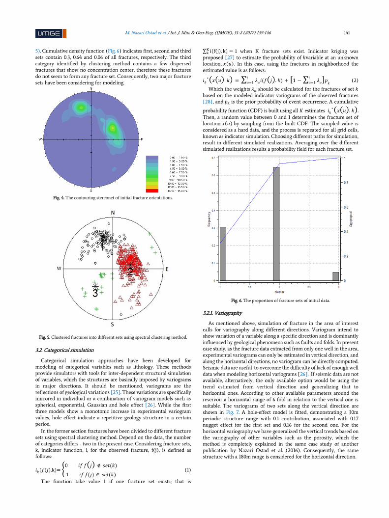
One problem associated with this method is that all fractures are allocated to the fracture sets, while in each set some of fractures do not seem to belong to that set. Therefore, the method should be modified to ignore outlier fractures. In the presented case, although according to the contour diagram (Fig. 4) two distinct fracture concentration centers exist, using spectral method fractures are clustered in 3 categories (Fig.

M. Nazari Ostad et al. / Int. J. Min. & Geo-Eng. (IJMGE), 51-2 (2017) 139-146 141

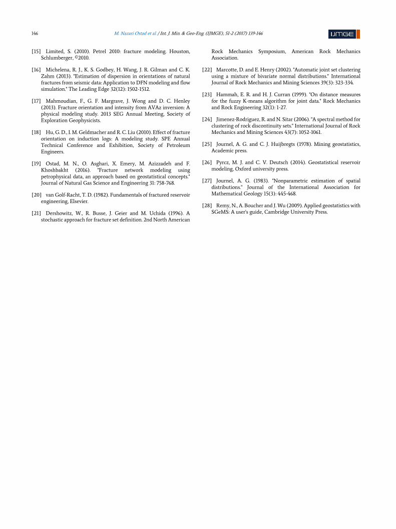
5). Cumulative density function (Fig. 6) indicates first, second and third sets contain 0.3, 0.64 and 0.06 of all fractures, respectively. The third category identified by clustering method contains a few dispersed fractures that show no concentration center, therefore these fractures do not seem to form any fracture set. Consequently, two major fracture sets have been considering for modeling.

Fig. 4. The contouring stereonet of initial fracture orientations.

Fig. 5. Clustered fractures into different sets using spectral clustering method.

3.2. Categorical simulation

Categorical simulation approaches have been developed for modeling of categorical variables such as lithology. These methods provide simulators with tools for inter-dependent structural simulation of variables, which the structures are basically imposed by variograms in major directions. It should be mentioned, variograms are the reflections of geological variations [25]. These variations are specifically mirrored in individual or a combination of variogram models such as spherical, exponential, Gaussian and hole effect [26]. While the first three models show a monotonic increase in experimental variogram values, hole effect indicate a repetitive geology structure in a certain period.

In the former section fractures have been divided to different fracture sets using spectral clustering method. Depend on the data, the number of categories differs - two in the present case. Considering fracture sets, k, indicator function, i, for the observed fracture, f(j), is defined as follows:

𝑖𝑘(𝑓(𝑗),k)= {0 𝑖𝑓 𝑓(𝑗) ∉ 𝑠𝑒𝑡(𝑘)

1 𝑖𝑓 𝑓(𝑗) ∈ 𝑠𝑒𝑡(𝑘) (1)

The function take value 1 if one fracture set exists; that is

∑ i(f(j). k) = 1Kk when K fracture sets exist. Indicator kriging was

proposed [27] to estimate the probability of 𝑘variable at an unknown location, 𝑥(𝑢). In this case, using the fractures in neighborhood the estimated value is as follows:

𝑖𝑘∗(𝑥(𝑢). 𝑘) = ∑ 𝜆𝛼𝑖(𝑓(𝑗). 𝑘)

𝑙𝛼=1 + [1 − ∑ 𝜆𝛼

𝑙𝛼=1

]𝑝𝑘 (2)

Which the weights 𝜆𝛼 should be calculated for the fractures of set 𝑘 based on the modeled indicator variograms of the observed fractures [28], and 𝑝𝑘 is the prior probability of event occurrence. A cumulative

probability function (CDF) is built using all 𝐾 estimates 𝑖𝑘∗(𝑥(𝑢). 𝑘).

Then, a random value between 0 and 1 determines the fracture set of location 𝑥(𝑢) by sampling from the built CDF. The sampled value is considered as a hard data, and the process is repeated for all grid cells, known as indicator simulation. Choosing different paths for simulation, result in different simulated realizations. Averaging over the different simulated realizations results a probability field for each fracture set.

Fig. 6. The proportion of fracture sets of initial data.

3.2.1. Variography

As mentioned above, simulation of fracture in the area of interest calls for variography along different directions. Variogram intend to show variation of a variable along a specific direction and is dominantly influenced by geological phenomena such as faults and folds. In present case study, as the fracture data extracted from only one well in the area, experimental variograms can only be estimated in vertical direction, and along the horizontal directions, no variogram can be directly computed. Seismic data are useful to overcome the difficulty of lack of enough well data when modeling horizontal variograms [26]. If seismic data are not available, alternatively, the only available option would be using the trend estimated from vertical direction and generalizing that to horizontal ones. According to other available parameters around the reservoir a horizontal range of 6 fold in relation to the vertical one is suitable. The variograms of two sets along the vertical direction are shown in Fig. 7. A hole-effect model is fitted, demonstrating a 30m periodic structure range with 0.1 contribution, associated with 0.17 nugget effect for the first set and 0.16 for the second one. For the horizontal variography we have generalized the vertical trends based on the variography of other variables such as the porosity, which the method is completely explained in the same case study of another publication by Nazari Ostad et al. (2016). Consequently, the same structure with a 180m range is considered for the horizontal direction.

142 M. Nazari Ostad et al. / Int. J. Min. & Geo-Eng. (IJMGE), 51-2 (2017) 139-146

Fig. 7. The variogram plots of 1st and 2nd fracture sets.

3.2.2. Sequential Indicator Simulation

The employed simulation process is Sequential Indicator Simulation (SIS). In this method each cell of gridded area take a value corresponding to the fracture set. Usually, numerous simulations are run (50 in this case), which their average over the individual cells results in a probability map of the study area. Note that each cell take a value between 0 and 1 representing the probability of the cell attachment to the simulated fracture set 𝑘. The same probability map could be gained for all sets. Here, because there are only 2 fracture sets, probability maps could be integrated in a single map (Fig. 8). The values near to 0 suggest higher probability for set 1, and the values near to 1 suggest higher probability for set 2.

Fig. 8. The probability map of fracture set; values close to 0 indicate higher

probability for 1st fracture set, and values close to 1 indicate higher probability for 2nd fracture set.

3.3. Orientation modeling

Orientation of a plane (fracture) could be specified by its Azimuth (ϕ) and dip (θ). Each one of fracture sets lies in a particular range of azimuth and dip. Using this characteristic, and what is obtained from the former sections, and regarding there are N cells in the grid, If ith cell contains n_i fracture, the following procedure is suggested for orientation modeling:

Plotting the azimuth cumulative probability function CDF(ϕ) according to the initial data and the proportions estimated in the former section in ith cell grid 1. Generating a random value; R(j)=rand[0,1] 2. Simulating azimuth value using R(j) and CDF(ϕ) 3. Simulating dip conditioned to the azimuth value 4. While j≤n_i, go to step 2 5. While i≤N, go to step 1

In the following subsection step 1 and 3 are explained in detail.

3.3.1. Azimuth and dip modeling in cells

CDF of azimuth in each cell grid is obtained using the initial data and the proportions simulated for each fracture set in section 3.2. The CDF of fracture azimuth in kth set can be describe in form of:

CDF(ϕk) = P(ϕmink < ϕ < ϕmax

k ) (3)

Therefore, If the estimated proportions of 1𝑠𝑡. 2𝑛𝑑. … fracture sets be denoted by 𝑝1. 𝑝2. … The CDF of azimuth in the cell would be:

𝐶𝐷𝐹(𝜙) = 𝑃(0 < 𝜙 < 360) = 𝑝1𝑃(𝜙𝑚𝑖𝑛1 < 𝜙 < 𝜙𝑚𝑎𝑥

1 ) + (𝑝1 +

𝑝2𝑃(𝜙𝑚𝑖𝑛2 < 𝜙 < 𝜙𝑚𝑎𝑥

2 )) + ⋯ = 𝑝1𝐶𝐷𝐹(𝜙1) + (𝑝1 + 𝑝2𝐶𝐷𝐹(𝜙2)) +

⋯ (4) Once 𝐶𝐷𝐹(𝜙) is calculated, the corresponding value to a random

number 𝑅(𝑗) is considered as the simulated value of fracture azimuth. In the present case, if the probabilities of the cell be 1, 0.65, 0.35 and 0, the CDF used for simulation would be as shown in Fig. 9. Using constructed CDFs corresponding azimuth value to 𝑅(𝑗) = 0.6 , for example, would be 82.1, 124.7, 338 and 343, respectively. When the azimuth of a fracture is simulated, dip thereupon is simulated conditioned to azimuth. For that, a dip value from 𝐶𝐷𝐹(𝜃 ∨ 𝜙) is generated using a random value.

Fig. 9. Blue lines: The CDF used for azimuth simulation when obtaining

different proportions equal to a) 1 b) 0.65 c) 0.35 d) 0; red lines: estimated azimuth corresponding to probability equal to 0.6.

3.3.2. Result of modeling

Stereonet and contour plots which are depicted in Fig. 10 and Fig. 11, respectively, illustrate the final scatter plots of simulated orientation. In comparison to the initial data stereonet and contour plots, it can be said that scatter plots of orientation are remarkably reproduced. Note that, as mentioned before only the major fracture sets are modeled, which means fracture set 3 is not modeled here.

Furthermore, this modeling procedure shows the capability of reproducing the proportions of main fracture sets. Fig. 12 compares the initial and simulated proportion of each fracture set, which are completely identical. In addition, quantile-quantile plot of initial dip versus simulated dip and also initial azimuth versus simulated azimuth depicted in Fig. 13a and Fig. 14a, respectively, show an accurate reproducing of dip and azimuth data. Finally, the fracture network that has been developed for the intra-well location is shown in Fig. 15a.

Fig. 10. The stereonet plot of simulated fractures.

M. Nazari Ostad et al. / Int. J. Min. & Geo-Eng. (IJMGE), 51-2 (2017) 139-146 143

Fig. 11. The contour stereonet diagram of simulated fractures.

Fig. 12. a) Initial proportion of main fracture sets; b) simulated proportion of main fracture set.

a) b)

Fig. 13. a) Q-Q plot of initial azimuth versus simulated azimuth, indicating an appropriate fracture azimuth reproducing by simulation; b) initial and simulated

azimuth histograms.

0 50 100 150 200 250 300 3500

50

100

150

200

250

300

350

simulated azimuth quantiles

initia

l azim

uth

quantile

s

Q-Q plot of initial azimuth vs simulated azimuth

0 100 200 300 4000

0.1

0.2

0.3

0.4

histogram of initial fracture azimuth

PD

F

Azimuth

0 100 200 300 4000

0.1

0.2

0.3

0.4

histogram of simulated fracture azimuth

PD

F

Azimuth

144 M. Nazari Ostad et al. / Int. J. Min. & Geo-Eng. (IJMGE), 51-2 (2017) 139-146

a) b)

Fig. 14. a) Q-Q plot of initial dip versus simulated dip, indicating an appropriate fracture dip reproducing by simulation; b) initial and simulated azimuth histograms.

3.4. Orientation modeling using Kent distribution

Fracture orientation is usually modeled through different distributions. One of the most useful models is Kent distribution which is a complicated model of Fisher-Bingham distribution in polar coordinates [11]. The pdf of Kent distribution when 𝜃 is the average of fracture set dip, and 𝜙 is the average of fracture azimuth is given by [14]: 𝐹(𝜃. 𝜙) = 𝑠𝑖𝑛𝜃𝑒𝑥𝑝 [𝜅𝑐𝑜𝑠𝜃 + 𝛽𝑠𝑖𝑛2𝜃(𝑐𝑜𝑠2𝜙 − 𝑠𝑖𝑛2𝜙)] (5)

𝐾 is concentration parameter which ranges between 0 and 100. A small value of 𝜅 results a wide scatter distribution and a high value of 𝜅 results a focused one. 𝛽 specifies the amount of anisotropy and its range is between 0 and 𝜅 2⁄ .

Also the orientation of fracture network is modeled in this paper, Using Kent distribution in order to compare its results with the results of proposed method. All of the fracture related variables including fracture length, density, and aperture are deemed identical, and it is only orientation that varies. The parameters for modeling two recognized fracture sets are summarized in Table 1. The stereonet plot of orientation values is illustrated in Fig. 16, which shows a weak reproducing of initial data.

Table 1. The parameters used for fracture orientation modeling.

𝑴𝒆𝒂𝒏(𝜽) 𝑴𝒆𝒂𝒏(𝝓) 𝜿 𝜷

𝑺𝒆𝒕𝟏 60 338.8 20 5

𝑺𝒆𝒕𝟐 40.4 77.8 20 10 a)

(a)

(b)

Fig. 15 The fracture network simulated by a) the suggested workflow, b) Kent distribution.

Fig. 16. The stereonet plot of simulated fractures using Kent distribution.

4. Connectivity

Fractures transfer the major part of fluid flow in fractured reservoirs. The transfer capacity is greatly influenced by the number of intersections occurs between fractures and thereby the orientation of them. These intersections make connections among different areas of reservoir, which in turn ease the transfer of stream toward producing wells. Therefore, estimating a true fracture network connectivity model

30 40 50 60 70 80 9030

40

50

60

70

80

90

simulated dip quantiles

init

ial d

ip q

uan

tile

sQ-Q plot of initial dip vs simulated dip

20 40 60 80 1000

0.05

0.1

0.15

0.2

histogram of initial fracture dip

PD

F

Dip

20 40 60 80 1000

0.05

0.1

0.15

0.2

histogram of simulated fracture dip

PD

F

Dip

M. Nazari Ostad et al. / Int. J. Min. & Geo-Eng. (IJMGE), 51-2 (2017) 139-146 145

is the ultimate function of a fracture network that reflects in a proper prediction of fluid flow.

In Fig. 17 the number of intersections in both developed method and modeling by Kent distribution is illustrated. By using Kent distribution the number of intersections increased dramatically which results in highly inter-connected fracture network. On the other hand, the developed method results a less inter-connected network. Although the authenticity investigation of them is not possible, the reconstruction of statistical parameters of our method shows that it may suggest a better prediction of fracture network connectivity.

(a)

(b)

Fig. 17. The number of intersections in grid cells using: a) the suggested

workflow, b) Kent distribution.

5. Conclusion

Orientation modeling highly influences the percolation degree in porous media. Applying a suitable model would change the paths of which the main stream happens, and even more would influence the amount of production in a reservoir. In this paper, a new approach for fracture orientation modeling is presented. Variograms, representing spatial structure in a geological medium, is modeled by a hole effect model, which shows repeatability in fracture sets. Afterwards, realizations of sequential indicator simulation employed for allocation of probability to each fracture set orientation on the cell grids. These probabilities thereafter used for construction of azimuth CDF through which azimuth could be simulated as a respond to a random number between 0 and 1. Following that, Dip angle is simulated conditioned to azimuth. The orientation model of suggested work-flow in comparison with built model using Kent distribution shows an accurate reproduction of initial data stereonet and histograms. In addition, the connectivity, a prominent factor in fluid flow simulation, of suggested method was less than the connectivity of modeling based on Kent distribution. The suggested method not only honors the statistical parameters but also could respect spatial parameters. In theory, SIS has shortcomings in producing high quality results, especially in case of 3 or more fracture sets. Therefore, for future studies it could be suggested to study the application of more robust techniques for geostatistical simulation of indicators which might produce more satisfactory result. In the case of azimuth and dip modeling in cells, one may produce numerous realizations to be able to measure the uncertainty of azimuth and dip simulation.

Acknowledgement

The authors are grateful to all professors whose constructive comments helped us to improve the manuscript.

REFRENCE

[1] Nelson, R. (2001). Geologic analysis of naturally fractured reservoirs, Gulf Professional Publishing.

[2] Sahimi, M. (2011). Flow and transport in porous media and fractured rock: from classical methods to modern approaches, John Wiley & Sons.

[3] Olarewaju, J., S. Ghori, A. Fuseni and M. Wajid (1997). Stochastic Simulation of fracture density for permeability field estimation. Middle East Oil Show and Conference, Society of Petroleum Engineers.

[4] Rafiee, A. and M. Vinches (2008). "Application of geostatistical characteristics of rock mass fracture systems in 3D model generation." International Journal of Rock Mechanics and Mining Sciences 45(4): 644-652.

[5] Liu, X., C. Zhang, Q. Liu and J. Birkholzer (2009). "Multiple-point statistical prediction on fracture networks at Yucca Mountain." Environmental geology 57(6): 1361-1370.

[6] Fadlelmula F, M. M., M. Fraim, J. He and J. E. Killough (2015). Discrete Fracture-Vug Network Modeling in Naturally Fractured Vuggy Reservoirs Using Multiple-Point Geostatistics: A Micro-Scale Case. SPE Annual Technical Conference and Exhibition, Society of Petroleum Engineers.

[7] Gauthier, B., A. Zellou, A. Toublanc, M. Garcia and J. Daniel (2000). Integrated fractured reservoir characterization: a case study in a North Africa field. SPE European Petroleum Conference, Society of Petroleum Engineers.

[8] Bourbiaux, B., R. Basquet, J. M. Daniel, L. Y. Hu, S. Jenni, G. Lange and P. Rasolofosaon (2005). "Fractured reservoirs modelling: a review of the challenges and some recent solutions." First Break 23(9): 33-40.

[9] Haddad, M., S. Srinivasan and K. Sepehrnoori (2015). Modeling natural fracture network using object-based simulation. 49th US Rock Mechanics/Geomechanics Symposium, American Rock Mechanics Association.

[10] Cacas, M. C., E. Ledoux, G. de Marsily, B. Tillie, A. Barbreau, E. Durand, B. Feuga and P. Peaudecerf (1990). "Modeling fracture flow with a stochastic discrete fracture network: Calibration and validation: 1. The flow model." Water Resources Research 26(3): 479-489.

[11] Kent, J. T. (1982). "The Fisher-Bingham distribution on the sphere." Journal of the Royal Statistical Society. Series B (Methodological): 71-80.

[12] Kent, J. T. and T. Hamelryck (2005). "Using the Fisher-Bingham distribution in stochastic models for protein structure." Quantitative Biology, Shape Analysis, and Wavelets 24: 57-60.

[13] Priest, S. D. (1993). Discontinuity analysis for rock engineering, Springer Science & Business Media.

[14] Peel, D., W. J. Whiten and G. J. McLachlan (2001). "Fitting mixtures of Kent distributions to aid in joint set identification." Journal of the American Statistical Association 96(453): 56-63.

146 M. Nazari Ostad et al. / Int. J. Min. & Geo-Eng. (IJMGE), 51-2 (2017) 139-146

[15] Limited, S. (2010). Petrel 2010: fracture modeling. Houston, Schlumberger, ©2010.

[16] Michelena, R. J., K. S. Godbey, H. Wang, J. R. Gilman and C. K. Zahm (2013). "Estimation of dispersion in orientations of natural fractures from seismic data: Application to DFN modeling and flow simulation." The Leading Edge 32(12): 1502-1512.

[17] Mahmoudian, F., G. F. Margrave, J. Wong and D. C. Henley (2013). Fracture orientation and intensity from AVAz inversion: A physical modeling study. 2013 SEG Annual Meeting, Society of Exploration Geophysicists.

[18] Hu, G. D., I. M. Geldmacher and R. C. Liu (2010). Effect of fracture orientation on induction logs: A modeling study. SPE Annual Technical Conference and Exhibition, Society of Petroleum Engineers.

[19] Ostad, M. N., O. Asghari, X. Emery, M. Azizzadeh and F. Khoshbakht (2016). "Fracture network modeling using petrophysical data, an approach based on geostatistical concepts." Journal of Natural Gas Science and Engineering 31: 758-768.

[20] van Golf-Racht, T. D. (1982). Fundamentals of fractured reservoir engineering, Elsevier.

[21] Dershowitz, W., R. Busse, J. Geier and M. Uchida (1996). A stochastic approach for fracture set definition. 2nd North American

Rock Mechanics Symposium, American Rock Mechanics Association.

[22] Marcotte, D. and E. Henry (2002). "Automatic joint set clustering using a mixture of bivariate normal distributions." International Journal of Rock Mechanics and Mining Sciences 39(3): 323-334.

[23] Hammah, E. R. and H. J. Curran (1999). "On distance measures for the fuzzy K-means algorithm for joint data." Rock Mechanics and Rock Engineering 32(1): 1-27.

[24] Jimenez-Rodriguez, R. and N. Sitar (2006). "A spectral method for clustering of rock discontinuity sets." International Journal of Rock Mechanics and Mining Sciences 43(7): 1052-1061.

[25] Journel, A. G. and C. J. Huijbregts (1978). Mining geostatistics, Academic press.

[26] Pyrcz, M. J. and C. V. Deutsch (2014). Geostatistical reservoir modeling, Oxford university press.

[27] Journel, A. G. (1983). "Nonparametric estimation of spatial distributions." Journal of the International Association for Mathematical Geology 15(3): 445-468.

[28] Remy, N., A. Boucher and J. Wu (2009). Applied geostatistics with SGeMS: A user's guide, Cambridge University Press.