1

CASE STUDY ON SEISMIC TUNNEL RESPONSE

By Stavroula Kontoe1

, Lidija Zdravkovic1, David M. Potts

1 and

Christopher O. Menkiti2

1 Imperial College, London

2 Geotechnical Consulting Group

Correspondence to:

Stavroula Kontoe

Department of Civil and Environmental Engineering

Skempton Building

South Kensington Campus, London, SW7 2AZ

Tel: +44(0)20 7594 5996, Fax: +44(0)20 7594 5934

Email: stavroula.kontoe@imperial.ac.uk

2

ABSTRACT:

This paper presents a case study of the Bolu highway twin tunnels that experienced a

wide range of damage during the 1999 Duzce earthquake in Turkey. Attention is

focused on a particular section of the left tunnel that was still under construction when

the earthquake struck and that experienced extensive damage during the seismic event.

Static and dynamic plane strain finite element (FE) analyses were undertaken to

investigate the seismic tunnel response at two sections and to compare the results with

the post-earthquake field observations. The predicted maximum total hoop stress

during the earthquake exceeds the strength of shotcrete in the examined section. The

occurrence of lining failure and the predicted failure mechanism compare very

favourably with field observations. The results of the dynamic FE analyses are also

compared with those obtain by simplified methodologies (i.e. two analytical elastic

solutions and quasi-static elasto-plastic FE analyses). For this example, the quasi-

static racking analysis gave thrust and bending moment distributions around the lining

that differed significantly from those obtained from full dynamic analyses. However,

the resulting hoop stress distributions were in reasonable agreement.

Key words: Bolu tunnels, Duzce earthquake, soil-structure-interaction, finite element

analysis

3

1.0 Introduction

Until recently, it was widely believed that underground structures are not

particularly vulnerable to earthquakes. However, this perception changed after the

severe damage and even collapse of a number of underground structures that occurred

during recent earthquakes (e.g. the 1995 Kobe, Japan earthquake, the 1999 Chi-Chi,

Taiwan earthquake and the 1999 Duzce, Turkey earthquake).

The present study considers the case of the Bolu highway twin tunnels that

experienced a wide range of damage during the 1999 Duzce earthquake in Turkey.

The Bolu tunnels establish a well-documented case, as there is information available

regarding the ground conditions, the design of the tunnels, the ground motion and the

earthquake induced damage. The focus in the present study is placed on a part of the

Bolu tunnels that was still under construction when the earthquake struck and that

suffered extensive damage.

The seismic response of circular tunnels has been the subject of a number of

studies. Owen and Scoll (1981) suggest that the response of circular tunnels to seismic

shaking can be described by the following types of deformation: axial compression or

extension, longitudinal bending and ovaling. Clearly, to describe all three modes of

tunnel deformation a three-dimensional model would be required. However, Penzien

(2000), among others, suggests that the most critical deformation of a circular tunnel

is the ovaling of the cross-section caused by shear waves propagating in planes

perpendicular to the tunnel axis. Hence, a number of simplified methods have been

developed to quantify the seismic ovaling effect on circular tunnels, which is

commonly simulated as a two-dimensional plane strain condition. The so called “free-

field deformation” approach ( e.g. St. John and Zahrah 1987) is based on the theory of

wave propagation in an infinite, homogeneous, isotropic, elastic medium and it

ignores any soil-structure interaction. Besides, there are various closed form solutions

(e.g. Hoeg 1968 and Schwartz and Einstein 1980, Penzien 2000), based on the theory

of an elastic beam on an elastic foundation, that consider the soil-structure-interaction

(SSI) effects in a quasi-static way, ignoring though any inertial interaction effects.

4

Both quasi-static and truly dynamic numerical modelling techniques (i.e. finite

differences, finite element and boundary element methods) are also widely used to

examine the seismic response of tunnels. An extensive review of the abovementioned

methods can be found in Hashash et al (2001).

In the present study, dynamic finite element analyses are employed to

investigate the seismic response of two sections of the Bolu tunnels. The results of the

dynamic FE analyses are then compared with field observations and with results

obtained by simplified methodologies (i.e. analytical elastic solutions and quasi-static

elasto-plastic FE analyses).

1.1 Construction details

The tunnels of interest are part of the Trans-European Motorway that links

Europe to the Middle East. They lie within the Gumusova-Gerede section, which is

between Ankara and Istanbul, where the motorway exists as a series of viaducts,

tunnels and embankments. The 23.7 km long Gumusova-Gerede section, which

crosses the Bolu Mountain, is constructed in complex ground conditions and includes

the 3.3 km long Bolu twin tunnels.

The construction of the Bolu twin tunnels started at the Asarsuyu (west) portal

in 1993 and at the Elmalik (east) portal in 1994. The twin tunnels were constructed as

four drives, two from each portal. The tunnel alignment is roughly “S” shaped in plan,

with the majority of the tunnel running north-south (Figure 1). Their cross-sections

range from 133m2 to 260m

2 to accommodate the changing ground conditions and they

are separated by a 50m wide rock/soil pillar. The maximum overburden cover is

250m, with most of the cross-sections under a cover of 100-150m. The ground

conditions along the tunnels alignment are highly variable, consisting of extremely

tectonised and sheared mudstones, siltstones and limestones, with thick layers of stiff

highly plastic fault gouge clay.

The initial design of the tunnels, based on the standard Austrian rock

classification system, adopted the New Austrian Tunnelling Method (NATM). This

technique is also known as the Sprayed Concrete Lining (SCL) method. With this

5

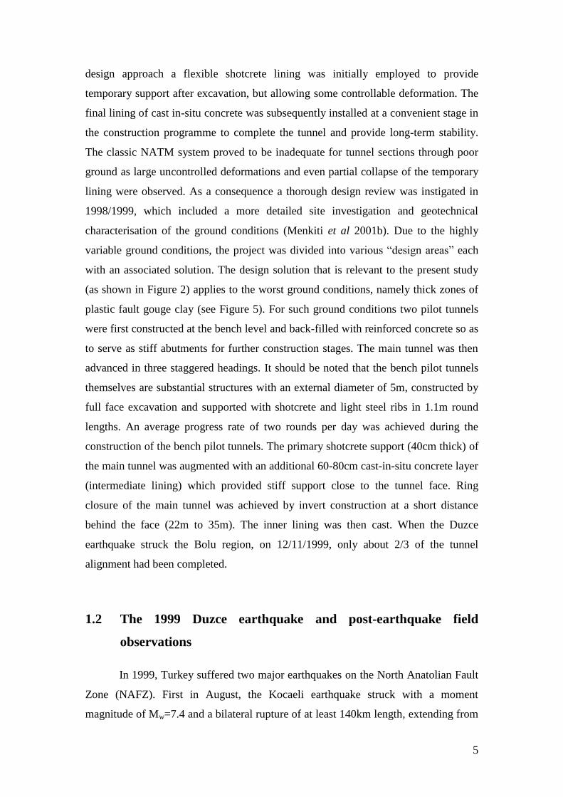
design approach a flexible shotcrete lining was initially employed to provide

temporary support after excavation, but allowing some controllable deformation. The

final lining of cast in-situ concrete was subsequently installed at a convenient stage in

the construction programme to complete the tunnel and provide long-term stability.

The classic NATM system proved to be inadequate for tunnel sections through poor

ground as large uncontrolled deformations and even partial collapse of the temporary

lining were observed. As a consequence a thorough design review was instigated in

1998/1999, which included a more detailed site investigation and geotechnical

characterisation of the ground conditions (Menkiti et al 2001b). Due to the highly

variable ground conditions, the project was divided into various “design areas” each

with an associated solution. The design solution that is relevant to the present study

(as shown in Figure 2) applies to the worst ground conditions, namely thick zones of

plastic fault gouge clay (see Figure 5). For such ground conditions two pilot tunnels

were first constructed at the bench level and back-filled with reinforced concrete so as

to serve as stiff abutments for further construction stages. The main tunnel was then

advanced in three staggered headings. It should be noted that the bench pilot tunnels

themselves are substantial structures with an external diameter of 5m, constructed by

full face excavation and supported with shotcrete and light steel ribs in 1.1m round

lengths. An average progress rate of two rounds per day was achieved during the

construction of the bench pilot tunnels. The primary shotcrete support (40cm thick) of

the main tunnel was augmented with an additional 60-80cm cast-in-situ concrete layer

(intermediate lining) which provided stiff support close to the tunnel face. Ring

closure of the main tunnel was achieved by invert construction at a short distance

behind the face (22m to 35m). The inner lining was then cast. When the Duzce

earthquake struck the Bolu region, on 12/11/1999, only about 2/3 of the tunnel

alignment had been completed.

1.2 The 1999 Duzce earthquake and post-earthquake field

observations

In 1999, Turkey suffered two major earthquakes on the North Anatolian Fault

Zone (NAFZ). First in August, the Kocaeli earthquake struck with a moment

magnitude of Mw=7.4 and a bilateral rupture of at least 140km length, extending from

6

Gölcük to Melen Lake. Three months later (12/11/1999), a second earthquake, known

as the Duzce earthquake, struck with a moment magnitude of Mw=7.2. The surface

rupture associated with the second event also propagated bilaterally in an east-west

direction, but was significantly smaller (40km) (Barka and Altunel, 2000). However,

GPS studies and radar interferometry studies suggest that the sub-surface slip

extended north-eastwards, beyond the eastern limits of the mapped surface rupture

(shown as dotted lines in Figure 1) (Lettis and Barka 2000).

The Bolu tunnels did not suffer any damage during the first event. Conversely,

due to the close proximity of the tunnels to the Duzce rupture, extensive damage in

various sections of the tunnels was observed after the second event. The west portals

of the Bolu tunnels are located within 3km from the east tip of the Duzce rupture and

within 20km from the earthquake’s epicenter. Ground motion records from the

November event close to the project site and to the causative fault are available from

the Duzce and the Bolu strong motion stations.

Due to the proximity of the project to the fault rupture, the ground motion at

the tunnels was presumably influenced by near fault effects. Although the Bolu

station motion is located at a distance of 18.3km from the surface rupture, it has some

features which are characteristic of near-field motions. In particular, Akkar and

Gülkan (2002) identified a strong pulse fling in the E-W Bolu accelerogram.

Furthermore, Sucuoğlu (2002) suggests that the short duration of the strong motion at

the Duzce station compared to Bolu indicates that the Bolu station was in the forward

directivity of the ruptured segment of the fault. The Bolu station is the closest

recording station to the Bolu Tunnels and its digital seismograph is mounted on an

isolated concrete pillar founded 2m into the sub-soil, reflecting the ground motion of a

soil layer with Vs=580m/s. It probably also very closely reflects the bedrock

(sandstone layer with Vs=1178m/s at a depth of 6.6m) ground motions. Taking also

into account the bilateral mechanism of the rupture and the relative positions of the

stations with respect to the project and the rupture (see Figure 1), it can be concluded

that the ground motion of the Bolu station is the most representative for the case

study. Since the causative fault generally runs in an east-west direction, the E-W and

N-S accelerograms represent the fault parallel and normal components of the motion

7

respectively. Furthermore, as one would expect for a lateral strike-slip fault, the

vertical component of the motion is significantly smaller (PGA=0.2g).

Due to the Duzce earthquake the Bolu tunnels experienced a wide range of

damage, depending on the ground conditions, the construction method and the

construction phase. Completed tunnels performed well, but in poor ground partly

completed tunnels, where only the initial support had been installed, suffered severe

damage and even collapse. Menkiti et al (2001a) and O’Rourke et al (2001) provide a

detailed description of the tunnels’ performance during the earthquake. The focus of

this paper is a zone of poor fault gouge clay where collapses occurred over a length

of 30m in both bench pilot tunnels (BPTs) of the Asarsuyu left drive (see Figure 4).

The BPTs were of 5m external diameter and provide a useful example for back-

analysis due to the completeness of the available information. The BPTs were in

pristine condition before the earthquake, having been constructed between 16th

October and 12 November 1999, with the Duzce earthquake occurring on the evening

of 12th

November 1999. When the Duzce earthquake struck, the BPTs of the Asarsuyu

left tunnel had not yet been back-filled with concrete and were only supported by

30cm thick shotcrete and HEB 100 steel ribs set at 1.1m longitudinal spacing. Figure

3a shows a picture of the partially collapsed left bench pilot tunnel (LBPT) during

post-earthquake repairs. The collapse is described as partial in the sense that although

the lining was very heavily damaged and deformed, it was not breached such that the

tunnel became in-filled with surrounding ground. Tunnel repairs comprised re-

excavating the damaged tunnel together with a surrounding annulus of soil, followed

by construction of a new pilot tunnel in the space created. Prior to commencement of

repairs, the damaged tunnel was carefully inspected and then stabilized by backfilling

it with foam concrete. This also served to preserve the structure of the damaged

tunnel, as shown in Figure 3, allowing further study during re-excavation. Excessive

deformation of the cross-section induced by the earthquake involved crushing of the

shotcrete and buckling of the steel ribs at shoulder and knee locations and invert uplift

up to 0.5m-1.0m. At some locations the buckled steel ribs shortened by up to 0.3-

0.4m. Figure 4 shows a plan view of the Asarsuyu left tunnel progress when the

earthquake struck. The bench pilot tunnels have a center-to-center separation of 19.0

8

m, and were being progressed with the left BPT leading the right one. The post-

earthquake investigations showed several interesting features of damage:

1. Damage was limited to the zone of fault gouge clay.

2. Severe damage and partial collapses were limited to the zone in which the two

BPTs overlap.

3. Damage was generally found to be more pronounced in the LBPT.

4. Interestingly, the leading portion of the LBPT in the same material (i.e. fault

gouge clay) did not collapse.

The present study employs two dimensional dynamic FE analyses to examine the soil-

structure interaction response at Sections A-B and C-D in Figure 4, with the objective

of explaining some of the observed damage.

1.3 Ground conditions

As noted previously, the design reassessment in 1998/1999 included a detailed

site investigation and geotechnical characterisation of the ground conditions. An

exploratory pilot tunnel was driven from each portal, which allowed detailed

characterisation of the ground conditions ahead of the main drives. Furthermore, the

ground investigation included sub-surface boreholes drilled from the pilot tunnels as

well as surface boreholes. The derived ground conditions for cross-sections AB and

CD are presented in Figure 5. The water table was established at a depth of 62m

below the ground surface.

Table 1 summarizes a description of the various geotechnical units and their

index properties. The strength properties (the angle of shearing resistance ΄, the

cohesion c΄ and the undrained strength Su) and the estimated maximum elastic shear

modulus (Gmax) values are listed in Table 2.

The strength properties of the two clay layers and the metasediments are based

on laboratory shear strength tests, as reported by Menkiti et al (2001a), while the

calcareous sandstone and the sandstone overlaying the bedrock were assumed to have

the same drained strength properties as the metasediments. Moreover, the estimated

9

maximum shear modulus (Gmax) values of the two clay layers and metasediments are

based on pressuremeter tests, as reported by Menkiti et al (2001a), while the Gmax

values of the two sandstones are based on the values published by O’Rourke et al

(2001).

1.4 Description of the numerical model

Plane strain analyses of the Bolu bench pilot tunnels (BPTs) were undertaken

for the cross sections AB (chainage 62+850) and CD (chainage 62+870) with the

finite element program ICFEP (Potts and Zdravkovic 1999). Figure 6 illustrates the

finite element mesh used in the analyses of the cross-section AB, which consists of

5574 8-noded quadrilateral solid elements and 62 3-noded beam elements. The FE

mesh models the ground stratigraphy down to the interface of the sandstone with the

quartzic rock (see Figure 5), which is a very stiff formation. The two-surface

kinematic hardening model (M2-SKH) of Grammatikopoulou et al (2006) was

employed to simulate the soil behavior in all the FE analyses. The M2-SKH model is

an extension of the Modified Cam Clay (MCC) model, as it introduces a small

kinematic yield surface within the MCC bounding surface and can therefore

reproduce soil hysteretic behaviour, which is important for dynamic analysis. The

model requires in total 7 parameters and their adopted values are given in the

Appendix.

To accurately represent the wave transmission through the finite element mesh,

it is necessary to ensure that the element size is small relative to the transmitted

wavelengths. Accordingly, the element side length (Δl) was chosen based on the

recommendation by Kuhlemeyer and Lysmer (1973) that:

[1] max

minS

f8

VΔl

where minSV is the lowest shear wave velocity that is of interest in the simulation and

maxf is the highest frequency of the input wave. Since in nonlinear problems the soil

stiffness changes during the analysis, an estimate of the minimum shear wave velocity

for each layer was obtained by undertaking equivalent linear analyses with the

10

software EERA (Bardet et al 2000), while the highest frequency was taken equal to

15Hz. The Fourier amplitude values of the uncorrected Bolu record in the high

frequency limit (e.g. greater than 10Hz) are almost zero and thus the choice of the

maximum cut-off frequency does not significantly affect the accuracy of the process.

The adopted shear stiffness-shear strain and damping-shear strain curves are presented

in the Appendix.

As previously mentioned various analytical studies suggest that the most

critical deformation of a circular tunnel is the ovaling of the transverse cross-section

caused by shear waves propagating in planes perpendicular to the tunnel’s axis. The

alignment of the Bolu tunnels is approximately perpendicular to the fault rupture.

Therefore, the Ε-W component of the ground motion, which is parallel to the fault

rupture, is the one responsible for the shear deformation of the tunnels' transverse

cross-section and was employed in all dynamic FE analyses.

As shown in Figure 5 the bedrock is located at a considerable depth from the

ground surface (193m and 185m for chainages 62+850 and 62+870 respectively).

Since there is no bedrock strong motion record in the vicinity of the tunnels, the

surface accelerogram was scaled to 70% to account for strong motion attenuation with

depth. The scaling factor (i.e. 0.7) adopted in this study is in agreement with the

recommendations of the Federal Highway Agency (FHWA, 2000) for depths of more

than 30m and is an upper bound for data collected from down-hole arrays (e.g.

Archuleta et al, 2000). Deconvolution analyses, assuming linear elastic soil behaviour,

were also performed both for the site of the Bolu station and for the site of the BPTs,

showing reduction factors of 0.85 and 0.5 respectively. However, since the bedrock at

the two sites differs, it was decided to finally adopt the FHWA, (2000)

recommendation of 0.7 which is close to the average value of the two deconvolution

analyses. In any case there is a degree of uncertainty in this approach which cannot be

avoided. A fourth order band-pass Butterworth filter was used to remove the extreme

low (below 0.1 Hz) and the high frequency components (above 15Hz) of the record.

Furthermore, there is no need to use the full duration of the seismic motion, as the

important shaking is limited to the time interval of 5sec-40sec. Figure 7 illustrates the

processed and scaled acceleration time history that was employed in all the dynamic

analyses, and the corresponding Fourier spectrum. The peak value of the input

11

acceleration time history is 0.57g (5.61m/sec2) and it occurs approximately 5.8 sec

after the onset of the excitation.

The width of the mesh and the lateral boundary conditions should be such that

free-field conditions (i.e. one-dimensional soil response) occur near to the lateral

boundaries of the mesh. After conducting a series of numerical tests (for details see

Kontoe, 2006), comparing the far-field 2D (i.e. with tunnels) response with the one

obtained from a 1D FE analysis (without any tunnels), the width of the mesh was

selected to be 219m and the tied degrees of freedom (TDOF) boundary condition was

applied along the vertical sides of the mesh. This boundary condition constrains nodes

of the same elevation on the two side boundaries to deform identically. In Kontoe

(2006) two more boundary conditions were examined for the lateral sides of the mesh:

the standard viscous boundary of Lysmer and Kuhlemeyer (1969) and the domain

reduction method in conjunction with the standard viscous boundary (Bielak et al

2003, Kontoe et al 2008b). The former method failed to reproduce the free-field

response and led to a serious underestimation of the response in the near field for a

mesh width of 219m. The latter method, which allows quantification of any wave

reflection from the lateral boundaries, showed that there were no significant wave

reflections from the lateral boundaries. Therefore it was concluded that the simple tied

degrees of freedom boundary condition could be used as it can successfully reproduce

the free-field response. The acceleration time history of Figure 7 was applied

incrementally in the horizontal direction to all nodes along the bottom boundary of the

FE model (i.e. along the bedrock-sandstone interface), while the corresponding

vertical displacements were restricted. The time integration was performed with the

Generalised-α method (Chung and Hulbert 1993) which is an unconditionally stable,

second order accurate scheme with controllable algorithmic dissipation (Kontoe et al

2008a). After conducting a series of numerical tests comparing 1D FE analyses with

equivalent linear EERA analyses the time step was selected to be t=0.01sec.

1.5 Modelling of construction sequence

When the earthquake struck, considerable static stresses were acting on the

tunnel linings due to the overburden pressure and the construction process. Hence,

12

prior to all 2D dynamic analyses presented in this study, a static analysis was

undertaken to establish the initial stresses acting on the lining. During the static

analysis displacements were restricted in both directions along the bottom mesh

boundary and horizontal displacements were restricted along the side boundaries.

Undrained behaviour was assumed for the clay units and drained conditions were

assumed for the rock layers.

As noted previously when the earthquake struck the BPTs were under

construction and they were therefore only supported by a 30cm thick preliminary

shotcrete lining with HEB 100 steel ribs set at 1.1m longitudinal spacing. While in a

3-dimensional model it is sensible to model the steel ribs, in plane strain analyses the

moment of inertia contribution from the steel ribs is very small compared to that

provided by the shotcrete. Therefore the steel ribs were ignored in all the analyses. It

should also be noted that at the time of the earthquake, the shotcrete had not yet

developed its full operational strength. Based on measured strength for the insitu

shotcrete development curves, the estimated strength and stiffness properties of the

tunnel linings at the instant of the earthquake at chainage 62+850 are listed in Tables

3 and 4 respectively.

The lining was modelled with beam elements, without using any interface

elements, and for all the analyses it was assumed to behave in a linear elastic manner.

The beam elements were generated within the mesh but deactivated at the beginning

of the analysis (i.e. in increment 0 which corresponds to the mesh generation stage).

The tunnel construction was modelled using the convergence-confinement method

which is described in detail by Potts and Zdravkovic (2001). Starting from a green-

field profile, the excavation of the tunnels causes stress relief in the ground. To model

this excavation process, equivalent nodal forces along the tunnel boundary, which

represent the stresses exerted by the excavated soil, are calculated and are then

removed over several increments of the analysis. During this process the elements

representing the excavated soil are non active. These forces are assumed to vary

linearly with the number of increments over which the excavation is to take place.

The excavation of the two BPTs was performed simultaneously in ten increments and

during the analysis the tunnels’ linings were activated, at the increment corresponding

to required stress relaxation, prior to the completion of excavation. In particular the

13

LBPT lining was constructed at 50% of stress relaxation (i.e. increment 5), whereas

the RBPT lining was constructed at 60% of stress relaxation (i.e. increment 6). The

higher value of stress relaxation assumed for the RBPT was used to account for the

fact that this tunnel was constructed after the LBPT and consequently in de-stressed

ground. For both tunnels an initial Young’s modulus of 5GPa was assigned which was

increased to 28GPa and to 21GPa for the LBPT and RBPT linings (see ) respectively

after the completion of excavation (i.e. increment 11). All the geometrical and

material properties of the BPTs linings are summarized in Table 5 and the coefficient

of earth pressure at rest profile is given in the Appendix (Figure A.1).

The static stresses acting on the tunnels’ lining caused an elliptical deformed

shape, which was slightly more pronounced in the RBPT. The amount by which the

tunnels deformed is summarized in Table 6. Measurements from monitoring the

exploratory pilot tunnel in a flyschoid clay (not at the sections considered herein)

reported by Menkiti et al (2001b) indicate a horizontal convergence of 15mm-25mm,

which is lower than the FE predictions of Table 6.. However, it is also reported that

the exploratory pilot tunnel experienced much larger movements in the fault gouge

clay. Furthermore, measurements from a completed section of the left tunnel (main

tunnel) in the gouge clay show a horizontal diametral convergence of the BPT

concrete beams of 0.9% (Menkiti et al, 2001b). Therefore, the FE results are generally

in good agreement with the observed static behaviour of the tunnels. The FE analysis

also indicates that the RBPT, which was constructed at 60% stress relaxation but is

more flexible than the LBPT (see ), experienced larger deformations. Figure 8 shows

the accumulated thrust (compression positive), bending moment and maximum hoop

stress distribution in the beam elements around the tunnels’ lining. The maximum

hoop stress distribution corresponding to the hoop stress at the extreme fibre of the

lining reflects the combined effect of the compressive thrust (T) and bending moment

(M) and it was calculated as follows:

[2] I

yM

A

TσH

where y is the distance from the neutral axis to the extreme fibre of the lining cross-

section and A is the area per unit width of the lining cross-section.

14

The thrust distribution is more or less uniform around the tunnel linings, while

the bending moment values are quite low and show a fluctuation around the lining.

Furthermore, the thrust and hoop stress distribution indicate that the LBPT attracted

higher loads than the RBPT. Menkiti et al (2001b), based on the performance of the

exploratory tunnel, estimated the immediate ground loads as being 40-65% of the

overburden, which corresponds to hoop stresses of 7450-12120kPa in the tunnels’

lining. The predicted hoop stresses for the RBPT lie within this range, while the ones

for the LBPT are marginally above the upper limit of this range. Figure 9 presents

contours of the pore water pressure distribution in the vicinity of the tunnels at the end

of the static analysis. The FE results show that the excavation process causes the

generation of pore water suctions. The contours of this tensile pressure are

concentrically aligned around the tunnels and they gradually decay with distance, so

that a compressive pore pressure is recovered at a distance from the tunnel linings

approximately equal to D/2 (i.e. D is the tunnel diameter).

1.6 2D nonlinear dynamic analyses

Once the static stresses acting on the tunnel linings were established, dynamic

analyses at chainages 62+850 and 62+870 were undertaken assuming that all

materials behaved in an undrained manner.

1.6.1 Chainage 62+850

Figure 10 compares the maximum shear strain profiles (caused only by the

dynamic excitation) at various distances x from the axis of symmetry of the 2D FE

model (i.e. x=0.0m, 13.0m and 50.0m) with the response of the corresponding 1D FE

model. It appears that the free-field response is recovered at a distance x=50.0m, as

the maximum shear strain profiles agrees well with the 1D results. Furthermore, the

response at the level of the tunnels (the centre of the tunnels is at z=160.0m) is

significantly de-amplified with respect to the free-field response at a distance

x=13.0m, while it is amplified in the pillar (i.e. x=0.0m).

The ovaling tunnel deformation suggested by various analytical studies was

verified by the FE analysis. Figure 11 illustrates an enlarged view of the deformed

15

mesh shortly after the peak of the excitation (i.e. at t=8.0sec). The ovaling

deformation is evident in both BPTs and it implies a stress concentration at the

shoulder and knee locations of the lining. Figure 12 illustrates contours of deviatoric

stress (J) in the vicinity of the tunnels (i.e. for the area indicated in Figure 11) at

various instances before and after the peak of the earthquake (i.e. at t=5.0, 6.0, 7.0 and

8.0 sec). Initially (i.e. at t=5.0) the stress contours have an almost vertical distribution,

later they gradually concentrate around the shoulder and knee locations of the linings.

Interestingly, shear planes at 45˚ seem to form in the pillar at t=8.0sec. Figure 13

presents the mobilised shear strength ratio (i.e. the ratio of the mobilised over the

available strength) distribution in the soil along the perimeter of the two BPTs for

t=5.0sec and for t=10.0sec. While the maximum mobilised strength ratio at t=5.0sec is

only 0.15, it reaches a value of 0.37 in the RBPT after the peak of the earthquake (i.e.

t=10.0sec). In any case it was observed that the mobilised strength ratio in the ground

around both BPTs was well below 1 throughout the analysis.

Figure 14 presents the accumulated pore water pressure and shear strain time

histories recorded at two integration points E (x=9.1m, z=157.4m) and F (x=-9.9m,

z=157.4m) adjacent to the crowns of the LBPT and the RBPT respectively. As

discussed in the previous section, the excavation process caused the generation of

pore water suction around the tunnel linings. During the first seconds of the

earthquake, the tensile pore pressure is maintained around both tunnels, but

approximately at the peak of the input excitation (see Figure 7a) an abrupt jump is

observed in Figure 14a, which results in a compressive pore pressure. Subsequently,

the compressive pore pressure continues to build up for a few more seconds

(approximately until t=10.0sec) and then stabilizes. It should be noted that for both

tunnels these stabilised values are lower than the prior to construction hydrostatic

pore pressure at the crown level (i.e. 936.0kPa). Furthermore the intense period of the

shaking generates significant permanent strains. The maximum shear strain adjacent

to the crown is 0.52% and 0.46% for the LBPT and the RBPT respectively. These

values are more than twice the maximum free-field shear strain at the same level (i.e.

at z=157.4m) which is 0.19% (see Figure 10).

Figure 15 shows the accumulated thrust (compression positive), bending

moment and maximum hoop stress distribution, due to the combined effects of static

16

and dynamic loading, in the beam elements around the BPTs’ lining at t=10.0sec. In

all three plots the distribution is highly non-uniform around the tunnel linings and the

maxima of the thrust, bending moment and maximum hoop stress occur at shoulder

and knee locations (i.e. θ=137˚ and 317˚ respectively). This is in exact agreement with

the post-earthquake field observations at the collapsed section of the LBPT, which

showed crushing of shotcrete and buckling of the steel ribs at shoulder (θ=137˚) and

knee (θ=317˚) locations of the lining (see Figure 3). Note that the photograph in

Figure 3 shows the view looking south. The plots in Figures 8, 12 and 14 show the

view looking North as indicated in section lines AB and CD in Figure 4. In Figure 14,

the hoop stresses at θ=137˚, 317˚ are approximately three times larger than the

corresponding static stresses in Figure 8, while in other locations the stresses are on

average two times larger. The thrust and bending moment time histories at θ=137˚ of

both BPTs are presented in Figure 16. In both tunnels, the axial forces start from an

initial value, induced by the static loading, and during the most intense period of

shaking they significantly increase. In a similar fashion to the pore pressure time

histories (see Figure 14), when the shaking intensity reduces the loads stabilise. While

the thrust developed in the RBPT is initially lower than that in the LBPT, during the

intense period of the shaking the thrust curves of the two BPTs become

indistinguishable. While the bending moment variations start from a very small initial

value, they significantly increase during the intense period of the earthquake and

finally stabilize to a relatively large value. It should be noted that the maximum and

stabilised values of bending moment in the RBPT are considerably lower than those

observed in the LBPT. Overall, the dynamic analysis results indicate that the LBPT

attracted higher loads than the RBPT. This is in agreement with post-earthquake field

observations suggesting that the LBPT experienced more severe damage than the

RBPT.

Table 7 summarizes the values of maximum hoop stress recorded at shoulder

and knee locations (i.e. at θ=137˚, 317˚) of the lining due to static and dynamic

loading. The predicted maximum total hoop stresses exceed the strength of the

shotcrete in both tunnels, which is 40MPa and 30MPa for the LBPT and RBPT

respectively (see ), and they thus match favourably with the observed failure.

However, it should be noted that the beam elements were assumed to behave as a

linear elastic material. Therefore the present FE analysis cannot actually model the

17

cracking of the lining and thus the predicted loads may differ to some extent from the

loads that were actually acting on it.

1.6.2 Chainage 62+870

As previously discussed, the Duzce earthquake caused striking damage to the

BPTs in the area that the two tunnels overlapped, but the leading portion of the LBPT

in the same material (i.e. fault gouge clay) did not suffer extensive damage (see

Figure 4). Two possible explanations were identified:

1. During the seismic event the BPTs presumably interacted, as the pillar

between the tunnels is small. Thus, wave reflections in the pillar possibly

caused amplification of the ground motion in the area where the BPTs

overlap.

2. The different stratigraphy of the cross section CD (i.e. at chainage 62+870)

resulted in lower seismic loads at the LBPT at this location compared to

those acting on it at the cross section AB (i.e. chainage 62+850).

To investigate these two postulations, two sets of analyses were undertaken. In the

first set of analyses, denoted in future discussions as 1BPT-AB, the analyses of the

cross-section AB at chainage 62+850 (denoted in future discussions as 2BPTs-AB)

were simply repeated without the RBPT (the stratigraphy is illustrated in Figure 5a

and only the LBPT was excavated). The purpose of this is to investigate whether the

two tunnels interacted during the seismic event by comparing the 1BPT-AB dynamic

analysis results with those previously obtained by the dynamic analysis 2BPTs-AB.

The second set of analyses, denoted in future discussions as 1BPT-CD,

concerns dynamic analyses of the stratigraphy of cross-section CD (see Figure 5b).

The purpose of this set of analyses is to examine whether the different stratigraphy

resulted in lower seismic loads in the LBPT at chainage 62+870 compared with those

predicted by the analysis 1BPT-AB. The finite element mesh used in the second set of

analyses, consists of 5274 8-noded quadrilateral solid elements and 31 3-noded beam

elements. The depth of the mesh for the cross section CD is 183.0m, while the width

was taken the same as before (i.e. 219.0m).

18

It should be noted that when the earthquake struck, the shotcrete at chainage

62+870 was 8 days old. In this set of analyses (i.e.1BPT-CD) the LBPT was

constructed at 60% stress relaxation and at the end of the excavation process was

assigned the material properties that correspond to the RBPT in Table 5 (as the

RBPT’s shotcrete at chainage 62+850 had similar age when the earthquake struck).

All other analysis arrangements (i.e. boundary conditions, time integration e.t.c.) were

kept the same as those used in the analyses of the cross section AB.

Figure 17 compares the maximum shear strain profiles (caused only by the

dynamic excitation) predicted by the three analyses (i.e. 2BPTs-AB, 1BPT-AB and

1BPT-CD) at x=70.0m and at x=0.0m. The free-field response (i.e. at x=70.0m)

obtained by the 2BPT-AB and 1BPT-AB analyses is very similar. This is not

surprising, since if the width of the mesh and the lateral boundaries have been

appropriately chosen, the free field response should not be affected by the structure.

On the other hand, the 1BPT-CD analysis predicts lower free-field response for the

fault gouge clay (i.e. layer 4) than the other two analyses. Hence, although the

thickness of the fault gouge clay layer is the same in all analyses, the response of the

gouge clay seems to be affected by the thickness of the overlaying layer (i.e.

metasediments). Conversely, the response of the other materials does not seem to be

significantly affected by the stratigraphy. Furthermore, in all analyses, the maximum

shear strain profile in the pillar at the level of the tunnel (i.e. the centre of the tunnel is

at z=160.0m and the centre of the pillar is at x=0m) is amplified with respect to the

corresponding free-field profile. However, the 1BPT-AB analysis predicts lower

amplification than the 2BPTs-AB analysis. This difference is quite small, but it

indicates that some interaction between the tunnels takes place in the 2BPTs-AB

analysis. Besides, the amplification is even lower in the 1BPT-CD analysis,

suggesting that the stratigraphy rather than the interaction of the tunnels is the crucial

parameter.

Figure 18 illustrates the first 20 seconds of the shear strain time histories

recorded at the integration points R (x=69.26m, z=160.7m, i.e. free-field location) and

S (x=0.235m, z=160.7m, i.e. pillar location) for the three analyses. Figure 18a shows

that the 1BPT-CD analysis gives consistently the lowest response, while the 1BPT-

AB and 2BPTs-AB analyses predict almost identical response. In the pillar, the

19

maximum shear strain predicted by the 2BPTs-AB analysis is 17% higher than the

one predicted by the 1BPT-AB analysis and 33% higher than the one predicted by the

1BPT-CD analysis. It should be noted that all analyses gave approximately the same

value of permanent shear strain at the end of the analysis.

Table 8 summarizes the predicted maximum hoop stress at the LBPT from the

three analyses. It is interesting to note that the 2BPTs-AB and 1BPT-AB analyses

predict the same total maximum hoop stress while that obtained by the 1BPT-CD

analysis is only 10% lower. Overall the 1BPT-CD analysis results show that the

LBPT was subjected to lower loads at chainage 62+870. However, the predicted

maximum hoop stress exceeds the 8-days shotcrete strength which is estimated to be

30.0 MPa. As discussed earlier, since the lining is modelled as a linear elastic

material, it is expected that all three analyses overestimate to some extent the loads

that were actually acting on it.

In conclusion, it was shown that the interaction of the BPTs and any potential

wave reflections in the pillar had only a minor effect on the seismic tunnel

performance. On the other hand, comparison of the 1BPTs-AB and 1BPT-CD

analyses showed that the differences in stratigraphy considerably affect the tunnel

response. However, these differences cannot fully explain the lack of serious damage

in the cross section CD. To further investigate this, a full 3D model and a more

realistic modelling of the tunnel linings would be needed.

1.7 Comparison with simplified methods of analysis

Due to the complexity and the high computational cost of dynamic FE

analyses, it is often preferred to employ simplified analytical solutions and/or quasi-

static FE methods to investigate the seismic response of tunnels. Although such

simplified methods cannot properly model the changes in soil stiffness and strength

that take place during an earthquake and they ignore any dynamic SSI effects, they

often give a reasonable estimate of the seismic loads. Commonly, dynamic SSI effects

are important for cases in which the dimensions of the cross-section are comparable

with the dominant wavelengths of the ground motion, for shallow burial depths and in

cases of stiff structures in soft soil. The dimensions and the burial depth in the

20

examined case study are such that the dynamic SSI effects are not expected to have

played a significant role in the collapse of the tunnels. Therefore, it is interesting to

examine how the results of these simplified methodologies compare with those

obtained by dynamic analysis presented for chainage 62+850 and with post-

earthquake field observations.

1.7.1 Comparison with analytical solutions

The extended Hoeg (Hoeg 1968 and Schwartz and Einstein 1980)3 and the

Penzien (2000) solutions, assuming either full-slip or non-slip conditions along the

interface between the ground and the lining, express the maximum thrust (Tmax) and

the maximum bending moment (Mmax) of the tunnel lining as a function of the

maximum free-field shear strain (γmax) at the level of the tunnel and properties of the

soil and the lining. The assumed parameters are listed in Table 9, while the γmax at the

level of the tunnels was taken from the 1D analysis with the M2-SKH model equal to

0.19% (see Figure 10). Furthermore, Tables 10 and 11 summarize the analytical

results for the LBPT and RBPT respectively.

The Penzien approach seems not to be so sensitive to the assumed condition

along the interface between the ground and the lining and in all cases predicts much

lower hoop stress values than those predicted by the extended Hoeg method. The field

observations indicated that the maximum hoop stress acting on the tunnels lining due

to static loading was on average 10MPa, the total hoop stress based on the Penzien

method is then 24.15MPa and 20.7MPa for the LBPT and the RBPT respectively.

These values are much lower than the estimated strength of shotcrete at the time of

the earthquake (40MPa and 30MPa for the LBPT and RBPT respectively).

Consequently, as failure was observed in the field, it can be concluded that the

Penzien (2000) methodology underestimates the maximum hoop stress developed due

to the earthquake in the BPTs. It should be noted that Hashash et al (2005) performed

quasi-static elastic FE analyses to validate the extended Hoeg and Penzien methods

3 The extended Hoeg solution was later summarised by Wang (1993) and it is often referred as the

Wang (1993) solution.

21

for non-slip conditions and they also concluded that the latter one significantly

underestimates the thrust in the tunnel lining for the condition of non-slip.

On the other hand, the extended Hoeg method gives much higher values of

maximum thrust for the no-slip assumption than for the full-slip assumption. The full-

slip condition is a reasonable approximation in cases of tunnels in soft soils, while for

tunnels in stiff soils (i.e. like the BPTs) it leads to underestimation of the maximum

thrust. It should be noted that the FE analyses presented herein are more consistent

with the no-slip assumption. This is because, as previously discussed, the mobilised

strength ratio of the soil at the tunnel-soil boundary was well below 1 throughout the

dynamic analysis (see Figure 13). For both BPTs the predicted seismic hoop stresses

by the extended Hoeg method under the no-slip assumption compare reasonably well

to those predicted by the FE analysis in Table 7 (i.e. compare earthquake values).

Furthermore, since the static hoop stress was on average 10MPa, the total

hoop stress acting on the lining based on the extended Hoeg method for the no-slip

assumption is then 36.8MPa and 32.8MPa for the LBPT and the RBPT respectively.

In conclusion, the extended Hoeg method, for the no-slip assumption, predicts hoop

stresses that match quite well with the post-earthquake field observations. On the

other hand the use of the Penzien solution for non-slip conditions should be avoided

as it severely underestimates the seismically induced maximum thrust

1.7.2 Quasi-static FE analyses

Usually, a quasi-static analysis approximates the earthquake induced inertia

forces as a constant horizontal body force applied throughout the mesh. In the present

study however, a different approach was followed. Initially a conventional static

analysis, as previously described, was undertaken to establish the static loads acting

on the tunnels. Once the construction sequence was modelled, the mesh was subjected

to simple shear conditions, as shown schematically in Figure 19. During the quasi-

static analysis the vertical displacements were restricted along all mesh boundaries,

while the horizontal displacements were restricted along the bottom boundary.

Furthermore, a uniform displacement us and a triangular displacement distribution, as

illustrated in Figure 19, were applied over 200 increments along the top and the lateral

boundaries of the mesh respectively. The displacement us was calculated as follows:

22

Hγu maxs =0.0019x195.0m=0.3705m

where H is the depth of the mesh and γmax is the maximum free-field shear strain at

the level of the tunnels calculated by the 1D dynamic analysis (see Figure 10).

Figure 20 illustrates the maximum (i.e. calculated at the last increment)

accumulated thrust, bending moment and hoop stress distribution around the tunnel

linings computed with the M2-SKH model. In a similar fashion to the results of the

corresponding dynamic analysis (see Figure 15) the load distribution is highly non-

uniform around the tunnel linings and the maxima of the thrust, bending moment and

hoop stress variations occur at shoulder and knee locations. Comparison of Figures 15

and 20 shows that the quasi-static analysis predicts lower values of thrust than the

dynamic analysis. Conversely, the quasi-static analysis predicts much higher bending

moments. The predicted hoop stress variation by the two analyses, which combines

the effect of the axial force and the bending moment, is fairly similar especially at

shoulder and knee locations.

While it is difficult to draw general conclusions from this set of analyses, it

seems that the quasi-static analysis’ results in terms of hoop stresses compare

reasonably well with those obtained by the corresponding dynamic analysis.

1.8 Conclusions

This paper presents a case study of the Bolu highway twin tunnels that

experienced a wide range of damage during the 1999 Duzce earthquake in Turkey.

Attention was focused on a particular section of the left tunnel that was still under

construction when the earthquake struck and that experienced extensive damage

during the seismic event. At the time of the earthquake only the two shotcrete

supported bench pilot tunnels (BPTs) had been constructed. The post-earthquake

investigations showed that the damage was limited to a zone of fault gouge clay

where the two tunnels overlapped. In the same material, the leading portion of the left

BPT (LBPT), where the adjacent RBPT had not been constructed, did not suffer

extensive damage.

23

Static and dynamic plane strain FE analyses were undertaken to investigate the

seismic tunnel response at two sections and to compare the results with the post-

earthquake field observations. The analyses of the first section (section AB) refer to

the area that the two BPTs overlap, while the analyses of the second section (section

CD) refer to the area where the leading portion of the LBPT did not experience severe

damage (Figure 4). The main purpose of the second set of analyses (i.e. section CD)

was to investigate why the leading portion of the LBPT tunnel did not experience

severe damage.

In the last part of the study the results of the dynamic analyses of section AB

were compared with those obtained by the simplified analytical elastic solutions using

the extended Hoeg (Hoeg 1968 and Schwartz and Einstein 1980) and Penzien (2000)

methods and those obtained by quasi-static FE elasto-plastic analyses in which free-

field racking deformation was imposed.

Several conclusions can be drawn from the results of the present study:

1. The tunnels deformed predominantly in an oval shape, with the maxima of the

thrust, bending moment and hoop stress occurring at shoulder and knee

locations of the lining. This is in agreement with post-earthquake field

observations at the severely damaged section of the LBPT (see Figure 3).

2. The numerical model depicted the observed failure at section AB, as the

maximum total hoop stress values exceed the strength of the shotcrete in both

tunnels. However, since the cracking of the lining was not modelled in the

present study, the predicted loads might deviate to some extent from the loads

that were actually acting on it.

3. It was shown that the interaction of the two BPTs and any wave reflections in

the pillar in between them only had a minor effect on their seismic

performance.

4. The observed differences in the seismic performance of the LBPT in sections

AB and CD can be partly attributed to the differences in stratigraphy between

the two locations.

24

5. The 2D FE analyses cannot fully explain the lack of serious damage in the

cross section CD, as the predicted maximum hoop stress exceeded the

shotcrete strength. To further investigate this, a full 3D model and a more

realistic modelling of the tunnel linings would be needed.

6. The extended Hoeg method, assuming no-slip between soil and lining,

predicts hoop stresses that match quite well with the dynamic FE analyses and

the post-earthquake field observations.

7. The Penzien (2000) method underestimated the maximum hoop stress

developed due to the earthquake in the BPTs. The use of the Penzien solution

for non-slip conditions should be avoided as it severely underestimates the

seismically induced maximum thrust. This is in agreement with the findings

of Hashash et al (2005).

8. The comparison of the quasi-static analysis results with those obtained from

the dynamic analyses showed significant differences in the thrust and bending

moment distributions around the lining, but the resulting hoop stress

distributions were in reasonable agreement.

25

1.9 Acknowledgements

The many contributors to the construction of Bolu Tunnels are acknowledged. The

Contractor was Astaldi-Bayindir JV, advised by Geoconsult and Lombardi S.A. The

Engineer was Yuksel-Rendel JV with input from GCG. The Employer was KGM. The

authors are also indebted to Profs Mair and O' Rourke who were colleagues on the

project.

1.10 References

Akkar, S., and Gülkan, P. 2002. A critical examination of near-field accelerograms

from the sea Marmara region earthquakes. Bulletin of the Seismological

Society of America, 92(1): 428-447.

Archuleta, R.J., Steidl, J.H., and Bonilla L.F. 2000. Engineering insights from data

recorded on vertical arrays. In Proceedings of the 12th World Conference in

Earthquake Engineering, 30 January- 4 February 2000, New Zealand, Paper

2681.

Bardet J.P., Ichii K., and Lin C.H. 2000). EERA, A computer program for Equivalent

linear Earthquake site Response Analysis of layered soils deposits. Report of

the University of Southern California, Los Angeles.

Barka A., and Altunel E. 2000. Preliminary report on whether the Asarsu valley is

active fault controlled. Report prepared for Astaldi-Bayindir Joint Venture.

Bielak J., Loukakis K., Hisada Y., and Yoshimura C. 2003. Domain Reduction

Method for Three-Dimensional Earthquake Modelling in Localized Regions,

Part I: Theory. Bulletin of the Seismological Society of America, 93(2):817-

824.

Chung J., and Hulbert, G.M. 1993. A time integration algorithm for structural

dynamics with improved numerical dissipation: the generalized-α method.

Journal of Applied Mechanics, 60: 371–375.

26

Federal Highway Administration (FHWA), 2000. Seismic retrofitting manual for

highway structures, part II. Report prepared by the Multidisciplinary Centre

for Earthquake and Engineering Research, Buffalo, New York.

Grammatikopoulou A. 2004. Development, implementation and application of

kinematic hardening models for overconsolidated clays. PhD thesis,

Department of Civil and Environmental Engineering, Imperial College,

London.

Grammatikopoulou A., Zdravkovic L., and Potts, D.M. 2006. General formulation of

two kinematic hardening constitutive models with a smooth elastoplastic

transition. International Journal of Geomechanics, 6 (5): 291-302.

Hashash Y.M.A., Hook J.J., Schmidt B., and Yao J.I-C., 2001. Seismic design and

analysis of underground structures. Tunnelling and Underground Space

Technology, 16(4): 247-293.

Hashash Y.M.A., Park D. and Yao J.I-C., 2005. Ovaling deformations of circular

tunnels under seismic loading, an update on seismic design and analysis of

underground structures. Tunnelling and Underground Space Technology,

20(5): 435-441.

Hoeg, K. 1968. Stresses against underground structural cylinders. Journal of Soil

Mechanics and Foundation Division, ASCE, 94(4): 833-858.

Kontoe S. 2006. Development of time integration schemes and advanced boundary

conditions for dynamic geotechnical analysis. PhD thesis, Department of Civil

and Environmental Engineering, Imperial College, London.

Kontoe S., Zdravković L., and Potts D.M. 2008a. An assessment of time integration

schemes for dynamic geotechnical problems. Computers and Geotechnics,

35(2): 253-264.doi:10.1016/j.compgeo.2007.05.001

Kontoe S., Zdravković L., and Potts D.M. 2008b. An assessment of the Domain

Reduction Method as an advanced boundary condition and some pitfalls in the

use of conventional absorbing boundaries. Accepted for publication in the

27

International Journal for Numerical and Analytical Methods in Geomechanics,

in press. doi:10.1002/nag.713

Kuhlemeyer R.L., and Lysmer J. 1973. Finite element method accuracy for wave

propagation problems. Technical Note, Journal of Soil Mechanics and

Foundation Division, ASCE, 99(5):421-427.

Lettis, W., and Barka A. 2000. Geologic characterisation of fault rupture hazard,

Gumusova-Gerede Motorway. Report prepared for the Astaldi-Bayindir Joint

Venture.

Lysmer J. and Kuhlemeyer R.L. 1969. Finite dynamic model for infinite media.

Journal of the Engineering Mechanics Division, ASCE, 95 (4): 859-877.

Menkiti C.O., Mair R.J., and Miles R. 2001b. Tunneling in complex ground

conditions in Bolu, Turkey. In the Proceedings of the Underground

Construction 2001 Symposium, London. pp.546-558.

Menkiti C.O., Sanders P., Barr J., Mair R.J., Cilingir, M. and James S. 2001a. Effects

of the 12th

November 1999 Duzce earthquake on the stretch 2 the Gumusova-

Gerede Motorway in Turkey. In the Proceedings of the International Road

Federation 14th

World Road Congress, Paris.

O’Rourke T.D., Goh S.H., Menkiti, C.O., and Mair R.J., 2001. Highway tunnel

performance during the 1999 Duzce earthquake. In the Proceedings of the

Fifteenth International Conference on Soil Mechanics and Geotechnical

Engineering, 27-31 August 2001, Istanbul, Turkey. Vol.2, pp. 1365-1368.

Balkema.

Owen G.N., and Scholl R.E., 1981. Earthquake engineering of large underground

structures. Report no. FHWA/RD-80/195, Federal Highway Administration

and National Science Foundation.

Penzien, J. 2000. Seismically induced racking of tunnel linings. International Journal

of Earthquake Engineering and Structural Dynamics, 29(5): 683-691.

28

Potts D.M., and Zdravković L.T. 1999. Finite element analysis in geotechnical

engineering: theory. Thomas Telford, London.

Potts D.M., and Zdravković L.T. 2001. Finite element analysis in geotechnical

engineering: application. Thomas Telford, London.

Schwartz, C.W., and Einstein, H.H. 1980. Improved Design of Tunnel Supports:

Vol.1- Simplified Analysis for Ground–structure Interaction in Tunneling.

UMTA-MA-06-0100-80-4, Urban Mass Transit Transportation

Administration, MA.

Seed H. B., Wong R. T., Idriss I. M., and Tokimatsu K. 1986. Moduli and damping

factors for dynamic analyses of cohesionless soils. Journal of the Geotechnical

Engineering Division, ASCE, 112(1): 1016-1032.

St. John C.M., and Zahrah T.F. 1987. Aseismic design of underground structures.

Tunnelling and Underground Space Technology, 2(2):165-197.

Sucuoğlu H., 2002. Engineering characteristics of the near-field strong motions from

the 1999 Kocaeli and Düzce Earthquakes in Turkey. Journal of Seismology.

6(1): pp. 347-355.

Vucetic M., and Dobry R., 1991. Effect of soil plasticity on cyclic response. Journal

of Geotechnical Engineering, ASCE, 117(1): 89-107.

Wang J.N. 1993. Seismic Design of Tunnels: A State-of-the-Art Approach.

Monograph 7, Parsons, Brinckerhoff, Quade and Douglas Inc, New York.

29

1.11 List of Figures

Figure 1: The surface rupture of the November 1999 Düzce earthquake and active

faults around Bolu

Figure 2: Design solution for the thick zones of fault gouge clay (after Menkiti et al

2001b)

Figure 3a: View of the damaged 5m diameter LBPT, stabilised by backfilling with

foam concrete. Picture taken during re-excavation and construction of a

replacement lining.

Figure 3b: Typical detail at location X between Ch 62+835 and 62+865 showing

damage to steel ribs within the shotcrete lining

Figure 4: Plan view of the Asarsuyu left drive showing the main tunnel and two bench

pilot tunnels under construction at the time of the earthquake

Figure 5: Ground profiles at chainage 62+850 (cross-section AB) (a) and at chainage

62+870 (cross-section CD) (b).

Figure 6: FE mesh configuration for chainage 62+850 after the excavation of the

tunnels

Figure 7: Scaled and truncated accelerogram used in the FE analyses (a) and

corresponding Fourier spectrum (b)

Figure 8: Accumulated thrust (a), bending moment (b) and maximum hoop stress (c)

distributions around the tunnels’ lining at the end of the static analysis

Figure 9: Contours of pore pressure distribution around the tunnels at the end of the

static analysis.

Figure 10: Maximum shear strain profile computed with the M2-SKH model for 1D

and 2D analyses

Figure 11: Enlarged view of the deformed mesh at t=8.0sec

30

Figure 12: Contours of deviatoric stress (J) (at t=5.0, 6.0, 7.0 and 8.0sec) in the

vicinity of the tunnels (for the area indicated in Figure 11)

Figure 13: Mobilised strength ratio along BPTs’ lining at t=5sec (a) and at t=10sec

Figure 14: Pore water pressure (a) and shear strain (b) time histories for integration

points adjacent to the crowns of the BPTs

Figure 15: Accumulated thrust (a), bending moment (b) and maximum hoop stress (c)

distribution around the tunnels’ lining at t=10.0sec

Figure 16: Thrust (a) and bending moment (b) time histories at θ=137˚ for both BPTs

Figure 17: Maximum shear strain profile computed with the 2BPTs-AB, the 1BPT-

AB and the 1BPT-CD model at x=70.0m (a) and at x=0.0m (b)

Figure 18: Shear strain time histories computed with the 2BPTs-AB, the 1BPT-AB

and the 1BPT-CD model at integration points R and S

Figure 19: Schematic representation of FE mesh configuration in quasi-static analysis

Figure 20: Accumulated thrust (a), bending moment (b) and maximum hoop stress (c)

distribution around the tunnels’ lining at the end of the quasi-static analysis

1.12 List of symbols

Bulk unit weight of soil.

max Maximum free-field shear strain.

A Area per unit width of the lining cross-section.

c’ Cohesion intercept of a soil.

E Young’s modulus.

maxf Maximum frequency of the input wave

31

G Shear modulus.

g(θ) Gradient of the yield function in the J- p΄ plane, as a function of

Lode’s angle.

gpp(θ) Gradient of the plastic potential function in the J- p΄ plane, as a

function of Lode’s angle.

I Moment of inertia.

J Deviatoric stress.

K0 Coefficient of earth pressure at rest.

M Bending moment in tunnel lining.

Mmax Maximum bending moment in tunnel lining.

p΄ Mean effective stress.

R Tunnel lining-soil racking ratio.

ρ Material density.

minSV Minimum shear wave velocity

Su Undrained strength

H Hoop stress

t Thickness of tunnel lining.

Thrust force in tunnel lining.

Tmax Maximum thrust in tunnel lining.

32

Δl Length of an element side.

Δt Incremental time step.

θ Lode’s angle.

ν Poisson’s ratio.

φ’ Angle of internal shearing resistance of a soil.

33

1.13 Figures

34

Figure 1: The surface rupture of the November 1999 Düzce earthquake and active faults around Bolu

35

Top heading

Shotcrete primary lining

Intermediate concrete lining

Inner concrete lining

Bench pilot tunnel with

infill concrete

Clearance

profile

Invert concrete

Bench

Invert

Scale

0 5m

Figure 2: Design solution for the thick zones of fault gouge clay (after Menkiti et al

2001b)

36

Figure 3b: Typical detail at location X between Ch 62+835 and 62+865 showing

damage to steel ribs within the shotcrete lining

Backfill

Foam Concrete

Previous Shotcrete

Shell

Buckled and sheared HEB

Steel Ribs

Invert heaved up to 0.5m

Detail X,

see Fig 3b

Figure 3a: View of the damaged 5m diameter LBPT, stabilised by backfilling

with foam concrete. Picture taken during re-excavation and construction of a

replacement lining.

Offset up to 0.4m

HEB Ribs

37

Figure 4: Plan view of the Asarsuyu left drive showing the main tunnel and two bench

pilot tunnels under construction at the time of the earthquake

38

83.0m

58.0m

37.0m

12.0m

5.0m

water table

Calcareous Sandstone

Metasediments

Fault Gouge Clay

Sandstone, Marl

Quarzitic Rock (bedrock)

Fault Breccia

and Fault Gouge Clay

19.0m

14.0m

RBPT LBPT

83.0m

44.0m

37.0m

14.0m

5.0m

water table

Calcareous Sandstone

Metasediments

Fault Gouge Clay

Sandstone, Marl

Quarzitic Rock (bedrock)

Fault Breccia

and Fault Gouge Clay

28.0m

LBPT

(a) (b)

Figure 5: Ground profiles at chainage 62+850 (cross-section AB) (a) and at chainage

62+870 (cross-section CD) (b).

20D=100m 20D=100m19m

195m

Calcareous Sandstone

Metasediments

Fault Gouge Clay

Sandstone, Marl

Fault Breccia

and Fault Gouge Clay

x

z

Figure 6: FE mesh configuration for chainage 62+850 after the excavation of the

tunnels

39

0 10 20 30 40

Time (sec)

-4

-2

0

2

4

6

Accele

ratio

n (

m/s

ec

2)

PGA=5.61m/sec2 at t=5.83sec

(a)

0.01 0.1 1 10

Frequency (Hz)

0

1

2

3

4

Fo

uri

er

Am

plit

ud

e (

m/s

ec)

(b)

Figure 7: Scaled and truncated accelerogram used in the FE analyses (a) and

corresponding Fourier spectrum (b)

0 60 120 180 240 300 360

Angle around tunnel lining,

10000

11000

12000

13000

14000

Ma

xim

um

Ho

op

Str

ess (

kP

a/m

)

0 60 120 180 240 300 360

Angle around tunnel lining,

-20

-10

0

10

20

Be

nd

ing M

om

en

t (k

Nm

/m)

0 60 120 180 240 300 360

Angle around tunnel lining,

2800

3200

3600

4000

Thru

st

(kN

/m)

LBPT

RBPT

(a)

(b)

(c)

Figure 8: Accumulated thrust (a), bending moment (b) and maximum hoop stress (c)

distributions around the tunnels’ lining at the end of the static analysis

40

CONTOUR LEVELSCOMPRESSION POSITIVE

875.0 kPa

426.0 kPa

-21.0 kPa

-471.0 kPa

-919.0 kPa

A

B

C

D

E

33.12m

18.7m RBPT

B

C

D

B

B

B

LBPTCC

B

B

B

B

BB

B BB B

B

C

B

D

E

EE

B

Figure 9: Contours of pore pressure distribution around the tunnels at the end of the

static analysis.

0 0.1 0.2 0.3

Maximum Shear Strain (%) (only due to e/q)

200

160

120

80

40

0

De

pth

(m

)

2D M2-SKH, x=50.0m

2D M2-SKH, x=13.0m

2D M2-SKH, x=0.0m

1D M2-SKH

Figure 10: Maximum shear strain profile computed with the M2-SKH model for 1D

and 2D analyses

41

26.0m

7.0m

Deformation scale: 0.08m

RBPT LBPT

Figure 11: Enlarged view of the deformed mesh at t=8.0sec

CONTOUR LEVELS

A

B

C

D

E

(a) t=5.0sec

CONTOUR LEVELS

A

B

C

D

E

(b) t=6.0sec

CONTOUR LEVELS

A

B

C

D

E

(c) t=7.0sec

CONTOUR LEVELS

A

B

C

D

E

(d) t=8.0sec

DD

D

C

D

D

D

C

C

BA

A

B

C

D

CD

D

C

C

D D

C

AA

B

BB

B

CD

B

B

CD

B

CD

B CC C

DB

B

B

B

C B CD

CCD

AB

C D C

B

A

A

B

C

C

C

BA

A

C

B

C

ABC

A

B CA B B

A

AB

C

A

A

BC

BC

A

A

BC

Figure 12: Contours of deviatoric stress (J) (at t=5.0, 6.0, 7.0 and 8.0sec) in the

vicinity of the tunnels (for the area indicated in Figure 11)

42

0 60 120 180 240 300 360

Angle around tunnel lining,

0

0.1

0.2

0.3

0.4

Mo

bili

se

d S

tre

ng

th R

atio

0 60 120 180 240 300 360

Angle around tunnel lining,

0

0.1

0.2

0.3

0.4

Mo

bili

se

d S

tre

ng

th R

atio

LBPT

RBPT

(a) t=5.0sec (b) t=10.0 sec

Figure 13: Mobilised strength ratio along BPTs’ lining at t=5sec (a) and at t=10sec

0 10 20 30 40

Time (sec)

-800

-400

0

400

800

Po

re P

ressure

(kP

a/m

)

LBPT

RBPT

0 10 20 30 40

Time (sec)

-0.6

-0.4

-0.2

0

0.2

0.4

Shea

r S

train

(%

)

LBPT

RBPT

(a) (b)

43

Figure 14: Pore water pressure (a) and shear strain (b) time histories for integration

points adjacent to the crowns of the BPTs

0 60 120 180 240 300 360

Angle around tunnel lining,

20000

24000

28000

32000

36000

40000

44000

Ma

xim

um

Ho

op

Str

ess (

kP

a/m

)

0 60 120 180 240 300 360

Angle around tunnel lining,

-300

-200

-100

0

100

200

Be

nd

ing M

om

en

t (k

Nm

/m)

0 60 120 180 240 300 360

Angle around tunnel lining,

6000

6400

6800

7200

7600

8000

Thru

st

(kN

/m)

LBPT

RBPT

(a)

(b)

(c)

Figure 15: Accumulated thrust (a), bending moment (b) and maximum hoop stress (c)

distribution around the tunnels’ lining at t=10.0sec

0 10 20 30 40

Time (sec)

2000

3000

4000

5000

6000

7000

8000

Thru

st (k

N/m

)

LBPT

RBPT

0 10 20 30 40

Time (sec)

-300

-200

-100

0

100

Ben

din

g m

om

en

t (k

Nm

/m)

=137°(a) (b)

44

Figure 16: Thrust (a) and bending moment (b) time histories at θ=137˚ for both BPTs

0 0.1 0.2 0.3

Maximum Shear Strain (%) (only due to e/q)

200

160

120

80

40

0D

epth

(m

)2BPTs-AB

1BPT-AB

1BPT-CD

(a) x=70.0m

0 0.1 0.2 0.3

Maximum Shear Strain (%) (only due to e/q)

200

160

120

80

40

0

Depth

(m

)

(b) x=0.0m

Figure 17: Maximum shear strain profile computed with the 2BPTs-AB, the 1BPT-

AB and the 1BPT-CD model at x=70.0m (a) and at x=0.0m (b)

0 4 8 12 16 20

Time (sec)

-0.3

-0.2

-0.1

0

0.1

0.2

Sh

ear

Str

ain

(%

)

2BPT-AB

1BPT-AB

1BPT-CD

0 4 8 12 16 20

Time (sec)

-0.3

-0.2

-0.1

0

0.1

0.2

She

ar

Str

ain

(%

)

2BPT-AB

1BPT-AB

1BPT-CD

(a) R (x=69.26m, z=160.7m) (b) S (x=0.2536m, z=160.7m)

Figure 18: Shear strain time histories computed with the 2BPTs-AB, the 1BPT-AB

and the 1BPT-CD model at integration points R and S

uff

usus

level of tunnels centre

Figure 19: Schematic representation of FE mesh configuration in quasi-static analysis

45

0 60 120 180 240 300 360

Angle around tunnel lining,

10000

20000

30000

40000

50000

Ma

xim

um

Ho

op

Str

ess (

kP

a/m

)

0 60 120 180 240 300 360

Angle around tunnel lining,

-400

-200

0

200

400

Be

nd

ing M

om

en

t (k

Nm

/m)

0 60 120 180 240 300 360

Angle around tunnel lining,

4000

5000

6000

7000

8000

Thru

st (k

N/m

)

LBPT

RBPT

(a)

(b)

(c)

Figure 20: Accumulated thrust (a), bending moment (b) and maximum hoop stress (c)

distribution around the tunnels’ lining at the end of the quasi-static analysis

0 400 800 1200 1600

200

160

120

80

40

0

Depth

(m

)

Su(kPa)

Calcareous Sandstone

Fault Breccia

Fault Gouge Clay

Metasediments

Fault Gouge Clay

Sandstone, Marl

Quartizic rock

(a) (b)

1 2 3 4 5

200

160

120

80

40

0

OCR

Ko

OC

Figure A.1: Undrained strength (Su) (a), overconsolidation ratio (OCR) and

coefficient of earth pressure at rest ( OC

OK ) (b) profiles.

46

0.001 0.01 0.1 1

Shear strain (%)

0

0.2

0.4

0.6

0.8

1

G/G

ma

x

Layer 1

Layer 2

Layer 3

Layer 4

Layer 5

Figure A.2: Shear stiffness-strain curves of different materials used in equivalent

linear analyses

0.0001 0.001 0.01 0.1 1 10

Shear strain (%)

0

4

8

12

16

20

Dam

pin

g r

atio (

%)

Seed et al (1986) (lower-bound)

Vucetic & Dobry (1991)

Figure A.3: Damping ratio-shear strain curves used in equivalent linear analyses

47

1.14 Tables

Table 1: Geotechnical description and index properties

Unit Consistency PI (%) CP

4 (%) &

Mineralogy

Calcareous

sandstone

Brown coloured slightly to

highly weathered/ fractured.

? ?

Fault breccia

and fault

gouge clay

heavily slicken-sided, highly

plastic, stiff to hard fault gouge

55 30-60

Metasediments Gravel, cobble and boulder

sized shear bodies in soil matrix.

10-15 5-25; illite

(58%),

smectite

(23%) Fault gouge

clay

Red to brown coloured, heavily

slicken-sided, highly plastic,

stiff to hard fault gouge

40-60 20-50,

smectite

Sandstone,

siltstone with

marl fragments

Gray sandstone with green,

weathered, medium strong to

weak marl fragments.

15 0-20

Bedrock Strong to very strong, faulted-

fractured quarzitic rock.

? ?

4 Clay percentage by weight.

48

Table 2: Estimated strength and stiffness parameters

Unit ΄ c΄ (kPa) Su

(kPa)

Gmax

(MPa) peak residual peak residual

Calcareous

sandstone 25˚-30˚ 20˚-25˚ 50 25 700 1000

Fault breccia

and fault gouge

clay

13˚-16˚ 9˚-12˚ 100 50 1000 750

Metasediments 25˚-30˚ 20˚-25˚ 50 25 1350 1500

Fault gouge clay 18˚-24˚ 6˚-12˚ 100 50 1000 850

Sandstone,

siltstone with

marl fragments

25˚-30˚ 20˚-25˚ 50 25 1500 2500

Table 3: Strength properties of the BPTs at the time of earthquake at chainage

62+850

Cube Strength

(fcu, MPa)

LBPT

(shotcrete15 days old )

RBPT

(shotcrete 7 days old )

40 30

49

Table 4: Stiffness properties of the BPTs just after construction and at the time of the

earthquake

LBPT RBPT

Age of shotcrete 1 day 15 days 1 day 7 days

Increment number 5 11 6 11

Young’s Modulus

(GPa) 5 28 5 21

Table 5: Geometrical and material properties of tunnel linings

t

(m)

I

(m4/m)

νl ρ

(Mg/m3)

C F

LBPT 0.3 0.00225

0.2 2.45 1.21 67.46

RBPT 0.3

0.00225

0.2 2.45 1.62 89.95

Table 6: Summary of the diametral movements and strains after the static analysis

Diametral

Convergence

LBPT RBPT

(mm) (%) (mm) (%)

Horizontal 40.72 0.81 51.86 1.03

Vertical 28.59 0.57 37.88 0.76

50

Table 7: Maximum hoop stress at shoulder and knee locations of the BPTs’ lining

computed with the M2-SKH model

Point

Maximum Hoop Stress ( Hσ ) (MPa)

Static Earthquake Total

LBPT, θ=137˚ 12.1 29.2 41.3

LBPT, θ=317˚ 12.5 29.0 41.5

RBPT, θ=137˚ 10.5 26.4 36.9

RBPT, θ=317˚ 10.5 29.6 40.1

Table 8: Maximum hoop stress developed at the LBPT for various analyses

Analysis

Maximum Hoop Stress ( Hσ ) (MPa)

Static Earthquake Total

2BPTs-AB 12.5 29.0 41.5

1BPT-AB 12.2 29.1 41.3

1BPT-CD 10.3 26.9 37.2

Table 9: Analytical methods parameters

Parameter Soil (layer 4) LBPT RBPT

Em (kPa) 2.21x106 - -

νm 0.3 - -

El (kPa) - 28.0 x106 21.0 x10

6

νl - 0.2 0.2

t (m) - 0.3 0.3

I (m4/m) - 0.00225 0.00225

51

r (m) - 5.0 5.0

Table 10: Summary of analytical results for the LBPT

LBPT Extended Hoeg Penzien (2000)

Full Slip No Slip Full Slip No Slip

Tmax (kN/m) 81.8 3959.2 81.9 163.2

Mmax (kNm/m) 204.6 204.6 204.6 204.0

Hσ max(MPa) 13.9 26.8 13.9 14.15

Table 11: Summary of analytical results for the RBPT

RBPT Extended Hoeg Penzien (2000)

Full Slip No Slip Full Slip No Slip

Tmax (kN/m) 61.7 3742.7 61.7 123.2

Mmax (kNm/m) 154.4 154.4 154.4 154.0

Hσ max(MPa) 10.5 22.8 10.5 10.7

Table A1: Material properties used for M2-SKH model

Layer λ κ v1 G

(MPa)

φ΄

1 0.2 0.02 3.2 1000.0 30˚

2 0.2 0.02 4.5 750.0 17˚

3 0.2 0.02 3.2 1500.0 30˚

4 0.2 0.02 4.5 850.0 17˚

5 0.2 0.02 3.2 2500.0 30˚

52

1.15 Appendix

1.15.1 Selection of M2-SKH model parameters

Five of the parameters required by the M2-SKH model have their origin in the

Modified Cam Clay (MCC) model. These are: three compression parameters (the

slope of the virgin compression line λ, the slope of the swelling line κ and the specific

volume at unit pressure v1 on the virgin compression line), one drained strength

parameter (φ΄) and one elastic parameter (the maximum shear modulus G). The values

of these parameters for the different layers are listed in Table A1. In the absence of

oedometer test data, typical values of compression parameters for stiff clays/ soft

rocks were chosen. Furthermore, the selected values of φ΄ are based both on the peak

strength variation of Table 2 and on geotechnical in-situ description of the different

units for the relevant cross-sections. Moreover, Potts and Zdravković, (1999) showed

that the above-mentioned input parameters of the MCC model and the initial state of

stress can be directly related to the undrained strength Su, as follows:

[A.1]

λ

κ

2NC

O

OC

O2NC

O

vi

u

B1OCRK21

K212B1K21

6

OCRθcosθg

σ

S

where viσ is the initial vertical effective stress, g(θ) is a function defining the shape of

the yield surface in the deviatoric plane, NC

OK is the value of the coefficient of earth

pressure at rest associated with normal consolidation, OC

OK is the current value of the

coefficient of earth pressure at rest, θ is the Lode’s angle, OCR is the

overconsolidation ratio defined as: vi

vm

σ

σOCR

, where vmσ is the maximum vertical

effective stress that the soil has been subjected to and B is defined as:

[A.2] NC

o

NC

o

K21)30g(

K13B

The estimated undrained strength for each layer is listed in Table 2. Employing

Equation [A.1] and the input parameters listed in Table A1 the initial stress state

53

parameters (OCR, Ko) can be selected to match the undrained strength values of Table

2 for the middle of each layer (assuming that the undrained strength varies linearly

with depth in each layer). Figure A.1 plots the assumed variation of Su with depth and

the resulting OCR and OC

OK profiles. It should also be noted that a linear variation of

suction is assumed above the water table.

The remaining 2 parameters (Rb, α) of the M2-SKH model define the

behaviour of the kinematic surface. To derive reliable values for the parameter Rb (i.e.

the ratio of the size of the bubble to that of the bounding surface), test data with

measurements of strains in the very small and small strain region are required. Since

no such data are available, the Rb is assumed to be 0.1 for the two clays and 0.15 for

the soft rock layers. Furthermore, the parameter α, which controls the decay of

stiffness, cannot be measured directly from the experimental data and is usually

determined by trial and error. However due to lack of data, a value of α equal to 15.0

was adopted for all layers based on Grammatikopoulou (2004).

1.15.2 Selection of equivalent linear elastic model parameters

Figure A.2 illustrates the shear stiffness degradation curves that were used for

each layer in the equivalent linear analyses. The shear stiffness variations of the clays

and metasediments were matched to data from pressuremeter tests. Since there was no

information available regarding the shear stiffness degradation of the sandstones (i.e.

layers 1 and 5), the two sandstones were assumed to have similar shear stiffness

degradation as the metasediments (i.e. layer 3). In addition the damping ratio curves

of Vucetic and Dobry (1991) for overconsolidated clays with a plasticity index of 50

were adopted for the two clay layers while for the remaining rock strata the lower

limit of the Seed et al’s (1986) range of damping ratio curves for sands was employed

(Figure A.3).