Cascadic Multilevel Methods

for Ill-Posed Problems

Lothar Reichel a,1,∗, Andriy Shyshkov a,1,

aDepartment of Mathematical Sciences, Kent State University, Kent, OH 44242,

USA.

Dedicated to Bill Gragg on the occasion of his 70th birthday.

Abstract

Multilevel methods are popular for the solution of well-posed problems, such ascertain boundary value problems for partial differential equations and Fredholmintegral equations of the second kind. However, little is known about the behav-ior of multilevel methods when applied to the solution of linear ill-posed problems,such as Fredholm integral equations of the first kind, with a right-hand side that iscontaminated by error. This paper shows that cascadic multilevel methods with aconjugate gradient-type method as basic iterative scheme are regularization meth-ods. The iterations are terminated by a stopping rule based on the discrepancyprinciple.

Key words: regularization, ill-posed problem, multilevel method, conjugategradient method

1 Introduction

Bill Gragg’s many contributions to scientific computing include work on ill-posed problems [9], iterative solution of symmetric, possibly indefinite linearsystems of equations [10], and Toeplitz matrices [1,2]. This paper is concernedwith all these topics.

∗ Corresponding author.Email addresses: reichel@math.kent.edu (Lothar Reichel),

ashyshko@math.kent.edu (Andriy Shyshkov).1 Research supported in part by an OBR Research Challenge Grant.

Preprint submitted to Elsevier Science 6 October 2008

Many problems in science and engineering can be formulated as a Fredholmintegral equation of the first kind

∫

Ω

κ(t, s)x(s)ds = b(t), t ∈ Ω. (1)

Here Ω denotes a compact Jordan measurable subset of R × . . . × R, andthe kernel κ and right-hand side b are smooth functions on Ω × Ω and Ω,respectively. The computation of the solution x of (1) is an ill-posed problembecause i) the integral equation might not have a solution, ii) the solutionmight not be unique, and iii) the solution – if it exists and is unique – does notdepend continuously on the right-hand side. The computation of a meaningfulapproximate solution of (1) in finite precision arithmetic therefore is delicate;see, e.g., Engl et al. [8] or Groetsch [11] for discussions on the solution ofill-posed problems. In the present paper, we assume that (1) is consistent andhas a solution in a Hilbert space X with norm ‖ · ‖. For instance, X may beL2(Ω). Often one is interested in determining the unique solution of minimalnorm. We denote this solution by x.

In applications, generally, not b, but a corrupted version, which we denote bybδ, is available. We assume that a constant δ > 0 is known, such that theinequality

‖bδ − b‖ ≤ δ (2)

holds. The difference bδ − b may, for instance, stem from measurement errorsand is referred to as “noise.”

Our task is to determine an approximate solution xδ of

∫

Ω

κ(t, s)x(s)ds = bδ(t), t ∈ Ω, (3)

such that xδ provides an accurate approximation of x. Equation (3) is notrequired to be consistent.

In operator notation, we express (1) and (3) as

Ax = b (4)

and

Ax = bδ, (5)

2

respectively. The operator A : X → Y is compact, where X and Y are Hilbertspaces. Thus, A has an unbounded inverse and may be singular. The right-hand side b is assumed to be in the range of A, denoted by R(A), but bδ

generally is not.

We seek to determine an approximation of the minimal-norm solution x of (4)by first replacing the operator A in (5) by an operator Areg that approximatesA and has a bounded inverse on Y , and then solving the modified equation soobtained,

Aregx = bδ. (6)

The replacement of A by Areg is referred to as regularization and Areg as aregularized operator. We would like to choose Areg so that the solution xδ of(6) is a meaningful approximation of x.

One of the most popular regularization methods is Tikhonov regularization,which in its simplest form is defined by

(A∗A + λI)x = A∗bδ, (7)

i.e., (Areg)−1 = (A∗A + λI)−1A∗. Here I is the identity operator and λ > 0 is

a regularization parameter. The latter determines how sensitive the solutionxδ of (7) is to perturbations in the right-hand side bδ and how close xδ is tothe solution x of (4); see, e.g., Engl et al. [8] and Groetsch [11] for discussionson Tikhonov regularization.

For any fixed λ > 0, equation (7) is a Fredholm integral equation of thesecond kind and, therefore, the computation of its solution is a well-posedproblem. Several two- and multi-level methods for the solution of the Tikhonovequation (7) have been described in the literature; see, e.g., Chen et al. [6],Hanke and Vogel [13], Huckle and Staudacher [15], Jacobsen et al. [16], andKing [17]. For a large number of ill-posed problems, these methods determineaccurate approximations of the solution of the Tikhonov equation (7) fasterthan standard (one-level) iterative methods.

The cascadic multilevel method of the present paper is applied to the un-regularized problem (5). Regularization is achieved by restricting the numberof iterations on each level using the discrepancy principle, defined in Section2. Thus, the operator Areg associated with the cascadic multilevel methodis defined implicitly. For instance, let the basic iterative scheme be CGNR(the conjugate gradient method applied to the normal equations). We applyCGNR on the coarsest discretization level until the computed approximatesolution satisfies the discrepancy principle. Then the coarsest-level solution isprolongated to the next finer discretization level and iterations with CGNR

3

are carried out on this level until the computed approximate solution satisfiesthe discrepancy principle. The computations are continued in this manner un-til an approximate solution on the finest discretization level has been foundthat satisfies the discrepancy principle. We remark that if the iterations arenot terminated sufficiently early, then the error in bδ may propagate to thecomputed approximate solution and render the latter a useless approxima-tion of x. We establish in Section 3 that the CGNR-based cascadic multilevelmethod is a regularization method in a well-defined sense.

The application of CGNR as basic iterative method in the multilevel methodis appropriate when A is not self-adjoint. The computed iterates live in R(A∗)and therefore are orthogonal to N (A), the null space of A. Here and through-out this paper A∗ denotes the adjoint of A.

When A is self-adjoint, the computational work often can be reduced by usingan iterative method of conjugate gradient (CG) type different from CGNR asbasic iterative method. Section 3 also describes multilevel methods for self-adjoint ill-posed problems based on a suitable minimal residual method.

The application of multigrid methods directly to the unregularized problem(5) recently also has been proposed by Donatello and Serra-Capizzano [7], whowith computed examples show the promise of this approach. The regulariza-tion properties of the multigrid methods used are not analyzed in [7].

Cascadic multilevel methods typically are able to determine an approximatesolution of (5) that satisfies the discrepancy principle with less arithmeticwork than application of the CG-type method, which is used for the basiciterations, on the finest level only. We refer to the latter method as a one-levelCG-type method, or simply as a CG-type method. A cascadic Landweber-based iterative method for nonlinear ill-posed problems has been analyzed byScherzer [22]. Numerical examples reported in [22] show this method to requiremany iterations.

Multilevel methods have for many years been applied successfully to the solu-tion of well-posed boundary value problems for partial differential equations;see, e.g., Trottenberg et al. [23] and references therein. In particular, a CG-based cascadic multigrid method has been analyzed by Bornemann and Deu-flhard [5]. However, the design of multilevel methods for this kind of problemsdiffers significantly from multilevel methods for ill-posed problems. This de-pends on that highly oscillatory eigenfunctions, which need to be damped,in the former problems are associated with eigenvalues of large magnitude,while they are associated with eigenvalues of small magnitude for the latterproblems.

This paper is organized as follows. Section 2 reviews CG-type methods and thediscrepancy principle. In particular, we discuss the regularization properties

4

of CG-type methods. Cascadic multilevel methods based on different CG-typemethods are described in Sections 3, where also regularization properties ofthese methods are shown. Section 4 presents a few computed examples andconcluding remarks can be found in Section 5.

2 CG-type methods and the discrepancy principle

Most of this section focuses on the CGNR method and its regularizing prop-erty. This method is suitable for the approximate solution of equation (5) whenA is not self-adjoint. At the end of this section, we review related results forCG-type methods for ill-posed problems with a self-adjoint operator A. Theregularization property of these methods is central for our proofs in Section 3of the fact that cascadic multilevel methods based on these CG-type methodsare regularization methods.

The CGNR method for the solution of (5) is the conjugate gradient methodapplied to the normal equations

A∗Ax = A∗bδ (8)

associated with (5). Let xδ0 denote the initial iterate and define the associated

residual vector rδ0 = bδ − Axδ

0. Introduce the Krylov subspaces

Kk(A∗A, A∗rδ

0) = spanA∗rδ0, (A

∗A)A∗rδ0, . . . , (A

∗A)k−1A∗rδ0 (9)

for k = 1, 2, 3, . . . . The kth iterate, xδk, determined by CGNR applied to (5)

with initial iterate xδ0 satisfies

‖Axδk − bδ‖ = min

x∈xδ0+Kk(A∗A,A∗rδ

0)‖Ax − bδ‖, xδ

k ∈ xδ0 + Kk(A

∗A, A∗rδ0), (10)

i.e., CGNR is a minimal residual method. Note that if xδ0 is orthogonal to

N (A), then so are all iterates xδk, k = 1, 2, 3, . . . . This is the case, e.g., when

xδ0 = 0. If in addition bδ is noise-free, i.e., if bδ is replaced by b in (10), then the

iterates xδk determined by CGNR converge to x, the minimal-norm solution of

(4).

Algorithm 1 describes CGNR. The computations can be organized so thateach iteration only requires the evaluation of one matrix-vector product withA and one with A∗. The algorithm is also referred to as CGLS; see Bjorck [4]for discussions on CGLS and LSQR, an alternate implementation.

5

Algorithm 1: CGNR

Input: A, bδ, xδ0, m ≥ 1 (Number of iterations);

Output: approximate solution xδm of (4);

rδ0 := bδ − Ax0; d := A∗rδ

0;k = 0;while k < m do

α := ‖A∗rδk‖

2/‖Ad‖2;xδ

k+1 := xδk + αd;

rδk+1 := rδ

k − αAd;β := ‖A∗rδ

k+1‖2/‖A∗rδ

k‖2;

d := A∗rδk+1 + βd;

k := k + 1;endwhile

The residual vector r = bδ − Ax is sometimes referred to as the discrepancyassociated with x. The discrepancy principle furnishes a criterion for choosingthe number of iterations, m, in Algorithm 1.

Definition (Discrepancy Principle). Let bδ satisfy (2) for some δ ≥ 0, andlet τ > 1 be a constant independent of δ. The vector x is said to satisfy thediscrepancy principle if ‖bδ − Ax‖ ≤ τδ.

We will be interested in reducing δ > 0, while keeping τ > 1 fixed, in theDiscrepancy Principle.

Stopping Rule 2.1 Let bδ, δ, and τ be the same as in the Discrepancy Prin-ciple. Terminate the iterations with Algorithm 1 when, for the first time,

‖bδ − Axδk‖ ≤ τδ. (11)

Denote the resulting stopping index by k(δ).

Note that generally k(δ) increases monotonically as δ decreases to zero withτ kept fixed. This depends on that the right-hand side bound in (11) getssmaller when δ decreases. Bounds for the growth of k(δ) as δ decreases areprovided by [12, Corollary 6.18].

An iterative method equipped with Stopping Rule 2.1 is said to be a regular-ization method if the computed iterates xδ

k(δ) satisfy

limδց0

sup‖b−bδ‖≤δ

‖x − xδk(δ)‖ = 0, (12)

where x is the minimal-norm solution of (4). We remark that the constantτ in Stopping Rule 2.1 is kept fixed as δ is decreased to zero. The followingresult, first proved by Nemirovskii [18], shows that CGNR is a regularization

6

method when applied to the solution of (5). A proof is also provided by Hanke[12, Theorem 3.12].

Theorem 2.2 Assume that equation (4) is consistent and that bδ satisfies(2) for some δ > 0. Terminate the iterations with Algorithm 1 according toStopping Rule 2.1, with τ > 1 a fixed constant. Let k(δ) denote the stoppingindex and xδ

k(δ) the associated iterate determined by CGNR. Then xδk(δ) → x

as δ ց 0, where x denotes the minimal-norm solution of (4).

We turn to the case when the operator A is self-adjoint. Let the kth iterate,xδ

k, be determined by a minimal residual method so as to satisfy

‖Axδk − bδ‖ = min

x∈xδ0+Kk(A,Arδ

0)‖Ax − bδ‖, xδ

k ∈ xδ0 + Kk(A, Arδ

0), (13)

with initial iterate xδ0 and rδ

0 = bδ −Axδ0. Note that the iterates are orthogonal

to N (A) provided that xδ0 is orthogonal to N (A). The following analog of

Theorem 2.2 holds.

Theorem 2.3 Let the operator A be self-adjoint, let equation (4) be consis-tent, and assume that bδ satisfies (2) for some δ > 0. Let the iterates xδ

k begenerated by a minimal residual method and satisfy (13). Terminate the iter-ations according to Stopping Rule 2.1, with τ > 1 a fixed constant. Let k(δ)denote the stopping index and xδ

k(δ) the associated iterate. Then xδk(δ) → x as

δ ց 0, where x denotes the minimal-norm solution of (4).

The above result is shown by Hanke [12, Theorem 6.15]. The case when A issemidefinite was first discussed by Plato [21]; see also Hanke [12, Chapter 3].

An implementation of a minimal residual method, referred to as MR-II, whichdetermines iterates xδ

k that satisfy (13) is provided by Hanke [12]. We use thisimplementation in computed examples of Section 4. The iterates (13) alsocan be determined by a simple modification of the MINRES algorithm byPaige and Saunders [19]. The computation of the iterate xδ

k defined by (13)requires k + 1 matrix-vector product evaluations with A. The exploitation ofself-adjointness of A generally reduces the number of matrix-vector productevaluations required to determine an iterate xδ

k that satisfies the discrepancyprinciple.

3 Multilevel methods based on CG-type iteration

In this section we present multilevel methods for the solution of (5). We firstdiscuss the use of CGNR as basic iterative method and show that with an

7

appropriate stopping rule, the multilevel method for the solution of (5) soobtained is a regularization method. The use of other CG-type methods asbasic iterative method in multilevel methods is discussed at the end of thissection.

Let S1 ⊂ S2 ⊂ . . . ⊂ Sℓ be a sequence of nested linear subspaces of L2(Ω)of increasing dimensions with Sℓ = L2(Ω). Each subspace is equipped with anorm, which we denote by ‖ · ‖. Introduce, for 1 ≤ i ≤ ℓ, the restriction andprolongation operators Ri : L2(Ω) → Si and Qi : Si → L2(Ω), respectively,with Rℓ and Qℓ identity operators, and define

bi = Rib, bδi

i = Ribδ, Ai = RiAQi.

When A is self-adjoint, it is convenient to choose Qi = R∗i , the adjoint of Ri.

Thus, Ai is the restriction of A to Si with Aℓ = A. It is convenient to considerthe noise in the restriction bδi

i of bδ to Si to be independent for 1 ≤ i ≤ ℓin the convergence proofs below. We therefore use the superscript δi for therestriction bδi

i of bδ. We require that there are constants ci, independent of δi,such that

‖bi − bδii ‖ ≤ ciδi, 1 ≤ i ≤ ℓ, (14)

for all δi ≥ 0, where ‖ · ‖ denotes the norm of Si. The coefficient ci dependson the norm of Si; this is illustrated by Remark 4.1 of Section 4. Below, wereduce the δi > 0, while keeping the ci fixed. We assume that the restrictionoperators Ri are such that δi = δi(δ) decrease as δ decreases with δi(0) = 0for 1 ≤ i ≤ ℓ. In the computations reported in Section 4, we let

δi = δ, 1 ≤ i ≤ ℓ. (15)

We also need prolongation operators Pi : Si−1 → Si for 1 < i ≤ ℓ. In thecomputed examples, we let the Pi be piecewise linear; see Section 4 for details.In addition, Algorithm 2 requires a mapping P1, such that P1(0) = 0 ∈ S1.

The “one-way” CGNR-based multilevel method of the present paper first de-termines an approximate solution of A1x = bδ1

1 in S1 by CGNR. The itera-tions with CGNR are terminated as soon as an iterate that satisfies a stoppingrule related to the discrepancy principle has been determined. This iterate ismapped from S1 into S2 by P2. We then apply CGNR to compute a correctionin S2 of this mapped iterate. Again, the CGNR-iterations are terminated by astopping rule related to the discrepancy principle. The approximate solutionin S2 determined in this fashion is mapped into S3 by P3. The computationsare continued in this manner until an approximation of x has been determinedin Sℓ. We refer to this scheme as Multilevel CGNR (ML-CGNR).

8

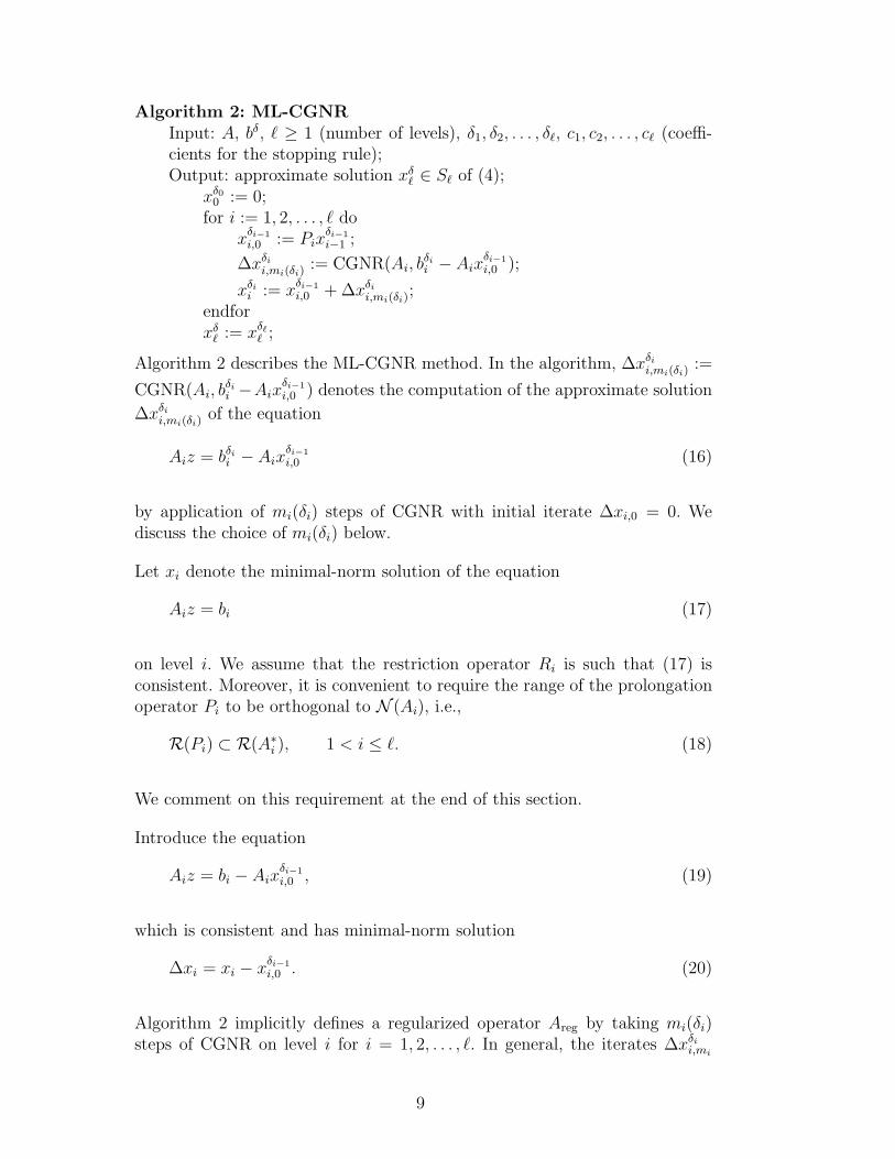
Algorithm 2: ML-CGNR

Input: A, bδ, ℓ ≥ 1 (number of levels), δ1, δ2, . . . , δℓ, c1, c2, . . . , cℓ (coeffi-cients for the stopping rule);Output: approximate solution xδ

ℓ ∈ Sℓ of (4);xδ0

0 := 0;for i := 1, 2, . . . , ℓ do

xδi−1

i,0 := Pixδi−1

i−1 ;

∆xδi

i,mi(δi):= CGNR(Ai, b

δii − Aix

δi−1

i,0 );

xδii := x

δi−1

i,0 + ∆xδi

i,mi(δi);

endforxδ

ℓ := xδℓ

ℓ ;

Algorithm 2 describes the ML-CGNR method. In the algorithm, ∆xδi

i,mi(δi):=

CGNR(Ai, bδii −Aix

δi−1

i,0 ) denotes the computation of the approximate solution

∆xδi

i,mi(δi)of the equation

Aiz = bδi

i − Aixδi−1

i,0 (16)

by application of mi(δi) steps of CGNR with initial iterate ∆xi,0 = 0. Wediscuss the choice of mi(δi) below.

Let xi denote the minimal-norm solution of the equation

Aiz = bi (17)

on level i. We assume that the restriction operator Ri is such that (17) isconsistent. Moreover, it is convenient to require the range of the prolongationoperator Pi to be orthogonal to N (Ai), i.e.,

R(Pi) ⊂ R(A∗i ), 1 < i ≤ ℓ. (18)

We comment on this requirement at the end of this section.

Introduce the equation

Aiz = bi − Aixδi−1

i,0 , (19)

which is consistent and has minimal-norm solution

∆xi = xi − xδi−1

i,0 . (20)

Algorithm 2 implicitly defines a regularized operator Areg by taking mi(δi)steps of CGNR on level i for i = 1, 2, . . . , ℓ. In general, the iterates ∆xδi

i,mi

9

do not converge to the minimal-norm solution (20) of (19) as the numberof iterations, mi, increases without bound; in fact, the norm ‖∆xi − ∆xδ

i,mi‖

typically grows with mi for mi sufficiently large. It is therefore important toterminate the iterations on each level after a suitable number of step.

Stopping Rule 3.1 Let the ci and δi be the same as in (14) and denote theiterates determined on level i by CGNR applied to the solution of (16) by∆xδi

i,mi, mi = 1, 2, . . . , with initial iterate ∆xi,0 = 0. Terminate the iterations

as soon as an iterate has been determined, such that

‖bδii − Aix

δi−1

i,0 − Ai∆xδii,mi

‖ ≤ τciδi, (21)

where τ > 1 is a constant independent of the ci and δi. We denote the termi-nation index by mi(δi) and the corresponding iterate by ∆xδi

i = ∆xδi

i,mi(δi).

The following theorem discusses convergence of the approximate solutions xδii

determined by Algorithm 2 on level i towards the minimal-norm solutions xi

of the noise-free projected problems (17). In particular, xδℓ

ℓ converges to x, theminimal-norm solution of the noise-free problem (4). A analogous result forequations (4) and (5) with a self-adjoint operator A, with CGNR replaced byMR-II in Algorithm 2 is shown towards the end of the section.

Theorem 3.2 Let Aℓ = A and bℓ = b. Assume that the equations (17) areconsistent for 1 ≤ i ≤ ℓ and that (18) holds. Let the projected contaminatedright-hand sides bδi

i satisfy (14). Terminate the iterations with CGNR in Al-gorithm 2 on levels 1, 2, . . . , ℓ according to Stopping Rule 3.1. This yields theiterates xδi

i for levels 1 ≤ i ≤ ℓ. Then the ML-CGNR method described byAlgorithm 2 is a regularization method on each level, i.e.,

limδiց0

sup‖bi−b

δii‖≤ciδi

‖xi − xδii ‖ = 0, 1 ≤ i ≤ ℓ, (22)

where xi is the minimal norm solution of (17) with xℓ = x.

Proof. We will show that for an arbitrary ǫ > 0, there are positive δ1, δ2, . . . , δℓ,depending on ǫ, such that

‖xi − xδii ‖ ≤ ǫ, 1 ≤ i ≤ ℓ. (23)

This then shows (22).

First consider level i = 1 and apply CGNR to the solution of

A1z = bδ11 .

10

By Theorem 2.2 there is a δ1 > 0, such that equation (23) holds for i = 1.

We turn to level i = 2. Since R(P2) is orthogonal to N (A2), the vector xδ12,0

has no component in N (A2). It follows from (14) that

‖b2 − A2xδ12,0 − (bδ2

2 − A2xδ12,0)‖ ≤ c2δ2.

Application of CGNR to (16) for i = 2 with initial iterate ∆x2,0 = 0 andStopping Rule 3.1 yields the approximate solution ∆xδ2

2 = ∆xδ22,m2(δ2). It follows

from Theorem 2.2 that we may choose δ2, so that

‖∆x2 − ∆xδ22 ‖ ≤ ǫ,

where ∆x2 is defined by (20). Using the definition of xδ22 in Algorithm 2, we

obtain (23) for i = 2. We now can proceed in this fashion for increasing valuesof i. This shows (23) for all i, and thereby the theorem. 2

Corollary 3.1 Let Aℓ = A, bℓ = b, bδℓ

ℓ = bδ, δℓ = δ, and cℓ = 1, where δ sat-isfies (2). Assume that R(Pℓ) ⊂ R(A∗). Let the products ciδi > 0, 1 ≤ i < ℓ,be fixed and large enough to secure that Stopping Rule 3.1 yields termina-tion of the iterations after finitely many steps on levels 1 ≤ i < ℓ. Thenthe ML-CGNR method described by Algorithm 2 with Stopping Rule 3.1 is aregularization method on level ℓ, i.e.,

limδց0

sup‖b−bδ‖≤δ

‖x − xδℓ‖ = 0, (24)

where xδℓ is the approximate solution determined by Algorithm 2 on level ℓ.

Proof. We first note that consistency of (17) holds for i = ℓ by the as-sumptions made in Section 1. The sole purpose of the computations on levels1 ≤ i < ℓ is to determine an initial approximate solution x

δℓ−1

ℓ,0 for level ℓ. We

are not concerned with how the iterates xδi

i on levels 1 ≤ i < ℓ relate to theminimal norm solutions of the systems (17) for 1 ≤ i < ℓ. Therefore property(18) only has to hold for i = ℓ. Since the systems (17) are not required to beconsistent for 1 ≤ i < ℓ, the right-hand sides in (21), i.e., the products ciδi,1 ≤ i < ℓ, have to be large enough to secure finite termination of the iterationson these levels. The corollary now follows from Theorem 2.2 or from the laststep (i = ℓ) of the proof of Theorem 3.2. 2

We turn to the situation when A is self-adjoint. Then CGNR is replaced byMR-II in Algorithm 2. We refer to the method so obtained as ML-MR-II.

Theorem 3.3 Let the conditions of Theorem 3.2 hold and assume that A isself-adjoint. Let the iterates xδi

i , 1 ≤ i ≤ ℓ, be generated by the ML-MR-

11

II method, i.e., by Algorithm 2 with CGNR replaced by MR-II. Terminate theiterations with MR-II in Algorithm 2 on levels 1, 2, . . . , ℓ according to StoppingRule 3.1 This yields the iterates xδi

i for levels 1 ≤ i ≤ ℓ. The ML-MR-II methodso defined is a regularization method on each level, i.e.,

limδiց0

sup‖bi−b

δii‖≤ciδi

‖xi − xδii ‖ = 0, 1 ≤ i ≤ ℓ,

where xi is the minimal norm solution of (17) with xℓ = x.

Proof. The result can be shown similarly as Theorem 3.2 by using the prop-erties of the iterates (13) collected in Theorem 2.3. 2

Corollary 3.2 Let Aℓ = A, bℓ = b, bδℓ

ℓ = bδ be as in Theorem 3.3 with δℓ = δ,and let the products ciδi, 1 ≤ i < ℓ, satisfy the conditions of Corollary 3.1.Assume that R(Pℓ) ⊂ R(A). Let the iterates xδi

i , 1 ≤ i ≤ ℓ, be generated bythe ML-MR-II method, i.e., by Algorithm 2 with CGNR replaced by MR-II.The ML-MR-II method so defined is a regularization method on level ℓ, i.e.,

limδց0

sup‖b−bδ‖≤δ

‖x − xδℓ‖ = 0, (25)

where xδℓ is the approximate solution determined by Algorithm 2 on level ℓ.

Proof. The result can be shown similarly as Corollary 3.1. 2

We conclude this section with a comment on the condition that R(Pℓ) beorthogonal to N (A). The other inclusions in (18) can be treated similarly.The conditions (18) are difficult to verify but have not been an issue in ac-tual computations; see Section 4 for further comments. Let PN (A) denote theorthogonal projector onto N (A). Then

xδℓ−1

ℓ,0 = (I − PN (A))xδℓ−1

ℓ,0 + PN (A)xδℓ−1

ℓ,0 .

The computation of xδℓ

ℓ from xδℓ−1

ℓ,0 in Algorithm 2 proceeds independently of

PN (A)xδℓ−1

ℓ,0 . We have

xδℓ

ℓ = (I − PN (A))xδℓ

ℓ + PN (A)xδℓ−1

ℓ,0 .

Hence,

limδց0

‖x − xδℓ

ℓ ‖ = ‖PN (A)xδℓ−1

ℓ,0 ‖,

12

CGNR ML-CGNR

δ‖b‖ m(δ)

‖xδ8,m(δ)

−x‖

‖x‖ mi(δ)‖xδ

8,m8(δ)−x‖

‖x‖

1 · 10−1 3 0.0934 2, 1, 1, 1, 1, 1, 1, 1 0.0842

1 · 10−2 4 0.0248 5, 5, 3, 2, 1, 1, 1, 1 0.0343

1 · 10−3 4 0.0243 8, 6, 6, 4, 3, 1, 1, 1 0.0243

1 · 10−4 11 0.0064 9, 13, 9, 9, 5, 4, 3, 2 0.0076

Table 1Example 4.1: Termination indices m(δ) for CGNR with Stopping Rule 2.1 deter-mined by δ and τ = 1.25, as well as relative errors in the computed approximatesolutions xδ

8,m(δ), and termination indices m1(δ),m2(δ), . . . ,mk(δ) for ML-CGNRwith Stopping Rule 3.1 determined by δ and c = 1.25, as well as relative errors inthe computed approximate solutions xδ

8,m8(δ).

i.e., we obtain an accurate approximation of x as δ ց 0 if PN (A)xδℓ−1

ℓ,0 is small.

We remark that in all computed examples of Section 4, PN (A)xδℓ−1

ℓ,0 is tiny.

4 Computed examples

This section compares ML-CGNR and ML-MR-II to one-level CGNR andMR-II, respectively. In the computed examples, the sets S1 ⊂ S2 ⊂ . . . ⊂ Sℓ

are used to represent discretizations of continuous functions in L2(Ω) withdim(Si) = ni. Specifically, in the first two examples Ω is an interval and Si isthe set of piecewise linear functions determined by interpolation at ni equidis-tant nodes. We may identify these functions with their values at the nodes,which we represent by vectors in R

ni equipped with the weighted Euclideannorm

‖v‖ =

1

ni

ni∑

j=1

(v(j))2

1/2

, v = [v(1), v(2), . . . , v(ni)]T ∈ Si. (26)

An inner product is defined similarly. Vectors with subscript i live in Rni . The

set Sℓ is used to represent functions on the finest level and is identified withR

nℓ . We let b = bℓ, x = xℓ, and A = Aℓ. The restriction operator Ri consists ofni rows of Iℓ, the identity matrix of order nℓ. It follows that RiR

∗i = Ii for all i.

All computations are carried out in Matlab with machine epsilon ǫ ≈ 2 ·10−16.

Example 4.1. Consider the Fredholm integral equation of the first kind

6∫

−6

κ(t, s)x(s)ds = b(t), −6 ≤ t ≤ 6, (27)

13

discussed by Phillips [20]. Its solution, kernel, and right-hand side are givenby

x(s) =

1 + cos(π3s), if |s| < 3,

0, otherwise,

κ(t, s) =x(t − s),

b(t) = (6 − |t|)(1 +1

2cos(

π

3t)) +

9

2πsin(

π

3|t|).

We discretize this integral equation by ℓ = 8 Nystrom methods based oncomposite trapezoidal quadrature rules with equidistant nodes. The numberof nodes on the ith level is ni = 4·2i+1; thus, there are 1025 nodes in the finestdiscretization. This yields the nonsymmetric matrix A = Aℓ ∈ R

1025×1025 andright-hand side b = bℓ ∈ R

1025. The condition number of the matrix A, definedby κ(A) = ‖A‖‖A−1‖ with ‖ · ‖ denoting the operator norm induced by thenorm (26) for i = ℓ, is about 1.9 · 1010, i.e., A is nearly numerically singular.There are only 9 nodes on the coarsest grid and the matrix A1 ∈ R

9×9 is notvery ill-conditioned; we have κ(A1) = 4.2 · 101.

In order to determine the “noisy” right-hand side bδ8 = bδ, we generate a vector

w with normally distributed entries with mean zero and variance one, definethe “noise-vector”

e = w‖b‖ · 10−η, (28)

for some η ≥ 0, and let

bδ = b + e. (29)

It follows from the strong law of large numbers that the noise level satisfies

‖b − bδ‖

‖b‖=

‖e‖

‖b‖≈ 1 · 10−η. (30)

We use the values

δ = δ1 = · · · = δℓ = ‖b‖ · 10−η (31)

in the Stopping Rules 2.1 and 3.1. Moreover, we let the coefficients ci in (21)be equal. Therefore, we generally omit the subscripts i of the δi and ci in (14)and (21) in this section.

14

Column 2 of Table 1 displays the number of iterations m(δ) required by (one-level) CGNR applied to A8x

δ8 = bδ

8 with initial iterate xδ8,0 = 0 to obtain

an approximate solution xδ8,m(δ) that satisfies Stopping Rule 2.1 for τ = 1.25

and different noise levels (30). Column 3 of the table shows the relative error‖xδ

8,m(δ)−x‖/‖x‖ in the computed approximate solutions. These columns showthe accuracy and the number of iterations to increase as the noise level isdecreased.

We turn to the ML-CGNR method implemented by Algorithm 2. The noisyright-hand side bδ is projected to the subspaces Si recursively to obtain thevectors bδ

i , 1 ≤ i ≤ 8. The jth component, (bδi )

(j), of bδi is given by

(bδi )

(j) = (bδi+1)

(2j−1), 1 ≤ j ≤ ni, 1 ≤ i ≤ 8. (32)

This defines the restriction operators Ri. The prolongation operators Pi aredefined by local averaging,

Pi =

1

1/2 1/2

1/4 1/2 1/4

1/2 1/2

1/4 1/2 1/4

1/2 1/2. . .

. . .. . .

1/4 1/2 1/4

1/2 1/2

1

∈ Rni×ni−1 .

The performance the ML-CGNR method implemented by Algorithm 2 withStopping Rule 3.1, determined by c = 1.25 and several values of δ, is illustratedby Table 1. The columns with header mi(δ) show, from left to right, thenumber of iterations required on the levels 1, 2, . . . , 8. Since for all i the matrixAi has four times as many entries as Ai−1, the dominating computational workis the evaluation of matrix-vector products on the finest discretization level.In this example, ML-CGNR reduces the number of iterations on the finestlevel to at most 1/3 of number of iterations required by one-level CGNR.

The last column of Table 1 displays the relative error in the computed ap-proximate solutions xδ

8,m8(δ) determined by Algorithm 2. The accuracy is seen

15

CGNR ML-CGNR

δ‖b‖ m(δ)

‖xδ8,m(δ)

−x‖

‖x‖ mi(δ)‖xδ

8,m8(δ)−x‖

‖x‖

1 · 10−1 2 0.3412 2, 1, 1, 1, 1, 1, 1, 1 0.2686

1 · 10−2 3 0.1662 2, 2, 1, 3, 1, 1, 1, 1 0.1110

1 · 10−3 3 0.1657 3, 3, 2, 1, 1, 1, 1, 1 0.1065

1 · 10−4 4 0.1143 4, 3, 3, 3, 2, 1, 1, 1 0.0669

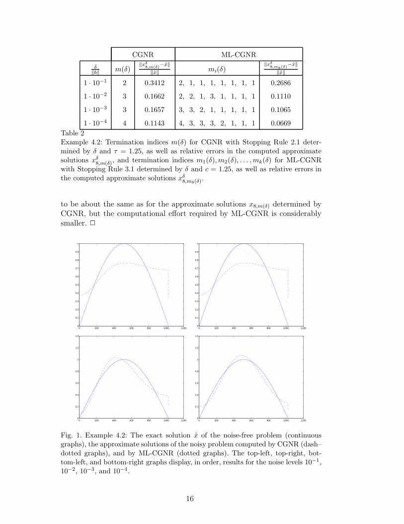
Table 2Example 4.2: Termination indices m(δ) for CGNR with Stopping Rule 2.1 deter-mined by δ and τ = 1.25, as well as relative errors in the computed approximatesolutions xδ

8,m(δ), and termination indices m1(δ),m2(δ), . . . ,mk(δ) for ML-CGNRwith Stopping Rule 3.1 determined by δ and c = 1.25, as well as relative errors inthe computed approximate solutions xδ

8,m8(δ).

to be about the same as for the approximate solutions x8,m(δ) determined byCGNR, but the computational effort required by ML-CGNR is considerablysmaller. 2

0 200 400 600 800 1000 12000

0.1

0.2

0.3

0.4

0.5

0.6

0.7

0.8

0.9

1

0 200 400 600 800 1000 12000

0.1

0.2

0.3

0.4

0.5

0.6

0.7

0.8

0.9

1

0 200 400 600 800 1000 12000

0.2

0.4

0.6

0.8

1

1.2

1.4

0 200 400 600 800 1000 12000

0.2

0.4

0.6

0.8

1

1.2

1.4

Fig. 1. Example 4.2: The exact solution x of the noise-free problem (continuousgraphs), the approximate solutions of the noisy problem computed by CGNR (dash–dotted graphs), and by ML-CGNR (dotted graphs). The top-left, top-right, bot-tom-left, and bottom-right graphs display, in order, results for the noise levels 10−1,10−2, 10−3, and 10−4.

16

Example 4.2. We consider the Fredholm integral equation of the first kind,

π/2∫

0

κ(s, t)x(s)ds = b(t), 0 ≤ t ≤ π, (33)

where κ(s, t) = exp(s cos(t)) and b(t) = 2 sinh(t)/t, discussed by Baart [3].The solution is given by x(t) = sin(t). We discretize (33) in the same wayas in Example 4.1 and use the same restriction and prolongation operatorsas in that example. Thus, the multilevel method uses eight levels, with thenonsymmetric matrix A = A8 ∈ R

1025×1025 representing the integral operatoron the finest discretization level. Matlab yield κ(A8) = 4.9 · 1021, i.e., thematrix A8 is numerically singular. The “noise” in bδ = bδ

8 is defined in thesame manner as in Example 4.1. Table 2 is analogous to Table 1 and showsthe performance of CGNR and ML-CGNR. The latter method is seen to yieldbetter approximations of x with less arithmetic effort.

Figure 1 displays the computed solutions for different noise levels. The con-tinuous graphs depict x, the dash-dotted graphs show approximate solutionsdetermined by CGNR, and the dotted graphs display approximate solutionsdetermined by ML-CGNR. The latter can be seen to furnish more accurateapproximations of x than the dash-dotted graphs for the same noise level.

The matrices Ai in the present example have “numerical null spaces” of co-dimension about eight. Hence, the matrices A2, A3, . . . , A8 have null spacesof large dimension. Nevertheless, accuracy of the computed solutions xδ

8 fordifferent noise levels is not destroyed by components in the null spaces of thematrices Ai; in fact, ML-MR-II is seen to yield higher accuracy than one-levelMR-II. 2

Remark 4.1 We are in a position to discuss the choice of constants ci = c in(14) and (21). Let the components of the vector w = [w(1), w(2), . . . , w(nk)]T ∈R

nk be normally distributed with mean zero and variance one. Then∑nk

j=1(w(j))2

has a Chi-square distribution with nk degrees of freedom.

Let the vector ei = bδi − bi consist of ni components of ek = bδ

k − bk. This isthe case in Examples 4.1 and 4.2, where ei = Riek. It follows from (28) thatthe components of ei can be expressed as

e(j)i = e

(ℓj)k = w(ℓj)‖bk‖ · 10−η, (34)

where w(ℓj) denotes an enumeration of the entries of w.

Let P· denote probability. Then it follows from (34) and the definition (31)of δ that

17

P‖bi − bδi‖ ≤ cδ=P‖ei‖

2 ≤ c2δ2

=P

1

ni

ni∑

j=1

(e(j)i )2 ≤ c2δ2

=P

ni∑

j=1

(w(ℓj))2 < c2ni

.

Using tables for Chi-square distribution, we find that on level i = 1 with 9nodes, the inequality (14) with c1 = c = 1.25 holds with a probability largerthan 74%. On level i = 2 with 17 nodes and c2 = c = 1.25, the inequality (14)holds with a probability larger than 78%. The probability of (14) being truefor i ≥ 3 with ci = c = 1.25 is much larger. We conclude that the probabilityof (14) to hold on every level can be increased by choosing more nodes on thecoarsest level and, of course, by increasing the values of the ci. 2

In Examples 4.1 and 4.2, we assumed that the error in the vectors bδi is caused

by the noise in bδ. This assumption is justified when there coarse level is fineenough to give a small discretization error. In the following example, this isnot the case.

Fig. 2. Example 4.3: The available blurred and noisy image.

Example 4.3. This example is concerned with image deblurring. This problemcan be thought of stemming from the discretization of an integral equation ofthe form (3) on a uniform grid by piecewise constant functions with Ω being

18

Fig. 3. Example 4.3: Image restored by ML-MR-II.

the unit square. The sets Si are made up of piecewise constant functions andare identified with vectors in R

ni.

The available blurred and noisy image, shown by Figure 2, is of size 817×817pixels. The blur is generated by the blurring operator A ∈ R

8172×8172defined by

the Matlab code blur.m from Regularization Tools by Hansen [14] with param-eters band= 33, sigma= 3. The block Toeplitz matrix A with banded Toeplitzblocks so obtained models blurring by a Gaussian point spread function withvariance sigma2 = 9. The parameter band specifies the half-bandwidth for theToeplitz blocks. The matrix A represents the blurring operator on the 4th andfinest grid, i.e., A4 = A. We also use the code blur.m to generate the matricesA1 ∈ R

1032×1032, A2 ∈ R

2052×2052, and A3 ∈ R

4092×4092that model the blurring

operator on coarser grids. We use different values of the parameter band inorder to get better approximation of A4 = A on the coarser grids. For A2 weuse band= 17, for A3 band= 9 and for A4 band= 5. All matrices Ai generatedare symmetric.

We define the perturbed right-hand side bδ4 by (29) with η = 1 · 10−2. The

projections bδi , i = 1, 2, 3, of bδ

4 onto the coarser grids are determined byconsidering each bδ

i a matrix with entries (bδi )

(s,t), i.e., (bδi )

(s,t) is the value ofpixel (s, t). The projections are now defined by

(bδi )

(s,t) = (bδi+1)

(2s−1,2t−1). (35)

19

This defines the restriction operators Ri.

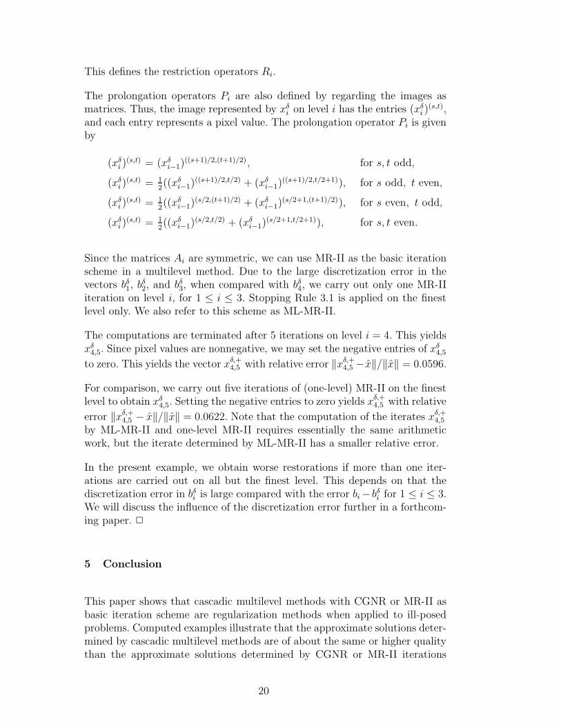
The prolongation operators Pi are also defined by regarding the images asmatrices. Thus, the image represented by xδ

i on level i has the entries (xδi )

(s,t),and each entry represents a pixel value. The prolongation operator Pi is givenby

(xδi )

(s,t) = (xδi−1)

((s+1)/2,(t+1)/2), for s, t odd,

(xδi )

(s,t) = 12((xδ

i−1)((s+1)/2,t/2) + (xδ

i−1)((s+1)/2,t/2+1)), for s odd, t even,

(xδi )

(s,t) = 12((xδ

i−1)(s/2,(t+1)/2) + (xδ

i−1)(s/2+1,(t+1)/2)), for s even, t odd,

(xδi )

(s,t) = 12((xδ

i−1)(s/2,t/2) + (xδ

i−1)(s/2+1,t/2+1)), for s, t even.

Since the matrices Ai are symmetric, we can use MR-II as the basic iterationscheme in a multilevel method. Due to the large discretization error in thevectors bδ

1, bδ2, and bδ

3, when compared with bδ4, we carry out only one MR-II

iteration on level i, for 1 ≤ i ≤ 3. Stopping Rule 3.1 is applied on the finestlevel only. We also refer to this scheme as ML-MR-II.

The computations are terminated after 5 iterations on level i = 4. This yieldsxδ

4,5. Since pixel values are nonnegative, we may set the negative entries of xδ4,5

to zero. This yields the vector xδ,+4,5 with relative error ‖xδ,+

4,5 −x‖/‖x‖ = 0.0596.

For comparison, we carry out five iterations of (one-level) MR-II on the finestlevel to obtain xδ

4,5. Setting the negative entries to zero yields xδ,+4,5 with relative

error ‖xδ,+4,5 − x‖/‖x‖ = 0.0622. Note that the computation of the iterates xδ,+

4,5

by ML-MR-II and one-level MR-II requires essentially the same arithmeticwork, but the iterate determined by ML-MR-II has a smaller relative error.

In the present example, we obtain worse restorations if more than one iter-ations are carried out on all but the finest level. This depends on that thediscretization error in bδ

i is large compared with the error bi − bδi for 1 ≤ i ≤ 3.

We will discuss the influence of the discretization error further in a forthcom-ing paper. 2

5 Conclusion

This paper shows that cascadic multilevel methods with CGNR or MR-II asbasic iteration scheme are regularization methods when applied to ill-posedproblems. Computed examples illustrate that the approximate solutions deter-mined by cascadic multilevel methods are of about the same or higher qualitythan the approximate solutions determined by CGNR or MR-II iterations

20

on the finest level only, but the computational effort required by multilevelmethods is lower.

Acknowledgment

We would like to thank Kazim Khan for discussions and comments.

References

[1] G. S. Ammar and W. B. Gragg, The generalized Schur algorithm for thesuperfast solution of Toeplitz systems, in Rational Approximation and itsApplications in Mathematics and Physics, J. Gilewicz, M. Pindor and W.Siemaszko, eds., Lecture Notes in Mathematics # 1237, Springer, Berlin, 1987315–330.

[2] G. S. Ammar and W. B. Gragg, Numerical experience with a superfast realToeplitz solver, Linear Algebra Appl. 121 (1989) 185–206.

[3] M. L. Baart, The use of auto-correlation for pseudo-rank determination in noisyill-conditioned least-squares problems, IMA J. Numer. Anal. 2 (1982) 241–247.

[4] A. Bjorck, Numerical Methods for Least Squares Problems, SIAM, Philadelphia,1996.

[5] F. A. Bornemann and P. Deuflhard, The cascadic multigrid method for ellipticproblems, Numer. Math. 75 (1996) 135–152.

[6] Z. Chen, Y. Xu, and H. Yang, A multilevel augmentation method for solvingill-posed operator equations, Inverse Problems 22 (2006) 155–174.

[7] M. Donatelli and S. Serra-Capizzano, On the regularization power of multigrid-type algorithms, SIAM. J. Sci. Comput. 27 (2006) 2053–2076.

[8] H. W. Engl, M. Hanke, and A. Neubauer, Regularization of Inverse Problems,Kluwer, Dordrecht, 1996.

[9] J. W. Evans, W. B. Gragg, and R. J. LeVeque, On the least squares exponentialsum approximation, Math. Comp. 34 (1980) 203–211.

[10] W. B. Gragg and L. Reichel, On the application of orthogonal polynomialsto the iterative solution of linear systems of equations with indefinite or non-Hermitian matrices, Linear Algebra Appl. 88–89 (1987) 349–371.

[11] C. W. Groetsch, The Theory of Tikhonov Regularization for FredholmEquations of the First Kind, Pitman, London, 1984.

21

[12] M. Hanke, Conjugate Gradient Type Methods for Ill-Posed Problems, Longman,Essex, 1995.

[13] M. Hanke and C. R. Vogel, Two-level preconditioners for regularized inverseproblems I: Theory, Numer. Math. 83 (1999) 385–402.

[14] P. C. Hansen, Regularization tools: A Matlab package for analysis and solutionof discrete ill-posed problems, Numer. Algorithms 6 (1994) 1–35.

[15] T. Huckle and J. Staudacher, Multigrid preconditioning and Toeplitz matrices,Electron. Trans. Numer. Anal. 13 (2002) 81–105.

[16] M. Jacobsen, P. C. Hansen, and M. A. Saunders, Subspace preconditionedLSQR for discrete ill-posed problems, BIT 43 (2003) 975–989.

[17] J. T. King, Multilevel algorithms for ill-posed problems, Numer. Math. 61(1992) 311–334.

[18] A. S. Nemirovskii, The regularization properties of the adjoint gradient methodin ill-posed problems, USSR Comput. Math. Math. Phys. 26(2) (1986) 7–16.

[19] C. C. Paige and M. A. Saunders, Solution of sparse indefinite systems of linearequations, SIAM J. Numer. Anal. 12 (1975) 617–629.

[20] D. L. Phillips, A technique for the numerical solution of certain integralequations of the first kind, J. ACM 9 (1962) 84–97.

[21] R. Plato, Optimal algorithms for linear ill-posed problems yield regularizationmethods, Numer. Funct. Anal. Optim. 11 (1990) 111–118.

[22] O. Scherzer, An iterative multi level algorithm for solving nonlinear ill-posedproblems, Numer. Math. 80 (1998) 579–600.

[23] U. Trottenberg, C. W. Osterlee, and A. Schuler, Multigrid, Academic Press,Orlando, 2001.

22