ill-posed inverse problems and regularization methods · ill-posed inverse problems and...

1

Ill-posed inverse problems and regularization methods

1. Inverse ill-posed problems: Examples

3. Theory of Regularization methods

2. Singular values and Pseudoinverse

4. Choosing the regularization parameters

5. Practical regularization methods

2

Examples of inverse problems

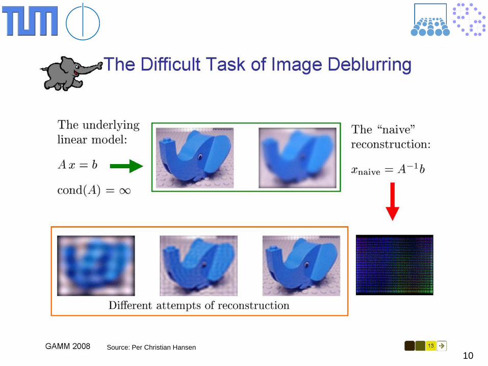
Image deblurring, image reconstruction

Ingredients: - Ill-conditioned (or singular) operator applied on data - added noise - recover original data as good as possible

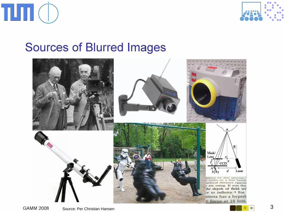
3 Source: Per Christian Hansen

4

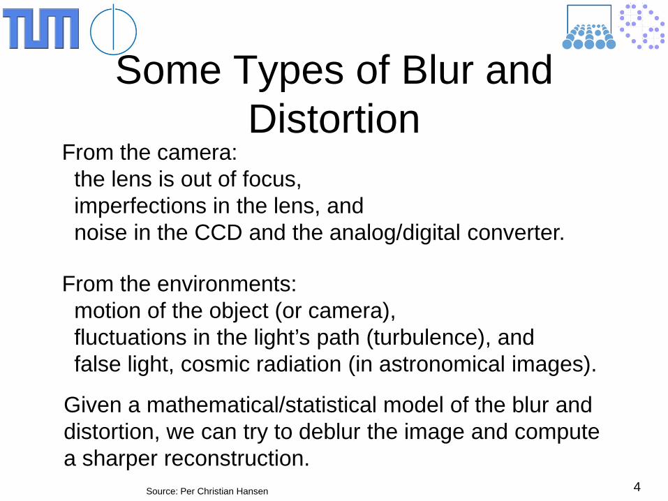
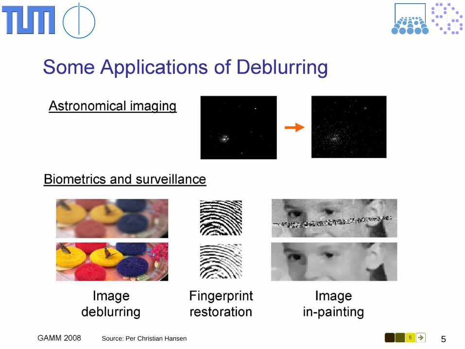
Some Types of Blur and Distortion

From the camera: the lens is out of focus, imperfections in the lens, and noise in the CCD and the analog/digital converter.

From the environments: motion of the object (or camera), fluctuations in the light’s path (turbulence), and false light, cosmic radiation (in astronomical images).

Given a mathematical/statistical model of the blur and distortion, we can try to deblur the image and compute a sharper reconstruction.

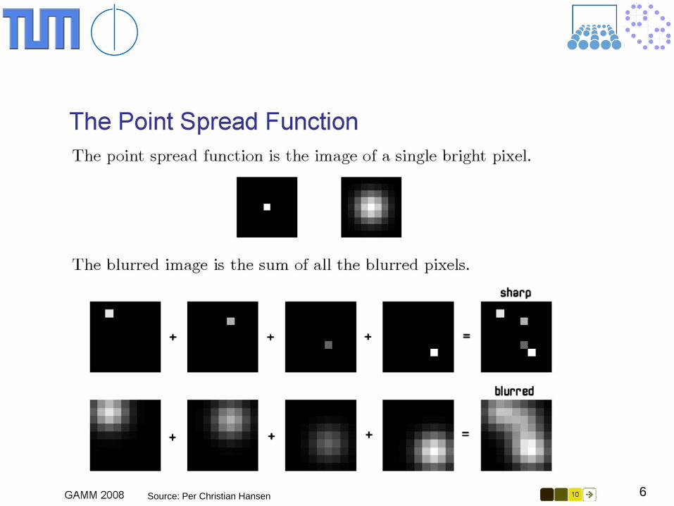
Source: Per Christian Hansen

7

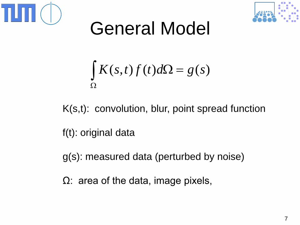
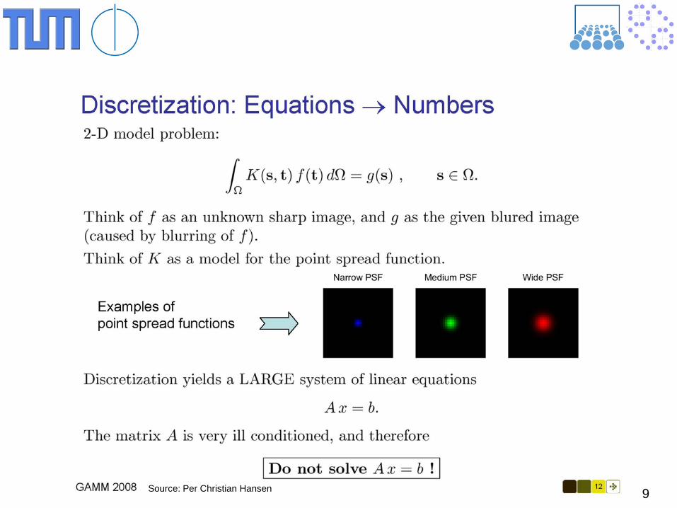
General Model

)()(),( sgdtftsK =Ω∫Ω

K(s,t): convolution, blur, point spread function f(t): original data g(s): measured data (perturbed by noise) Ω: area of the data, image pixels,

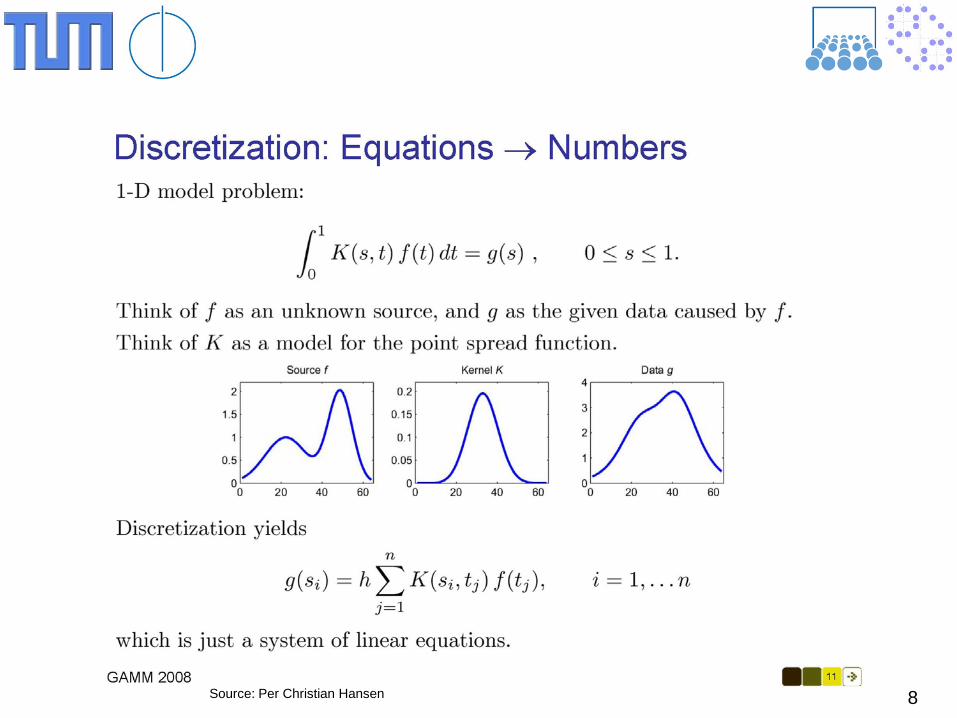
11

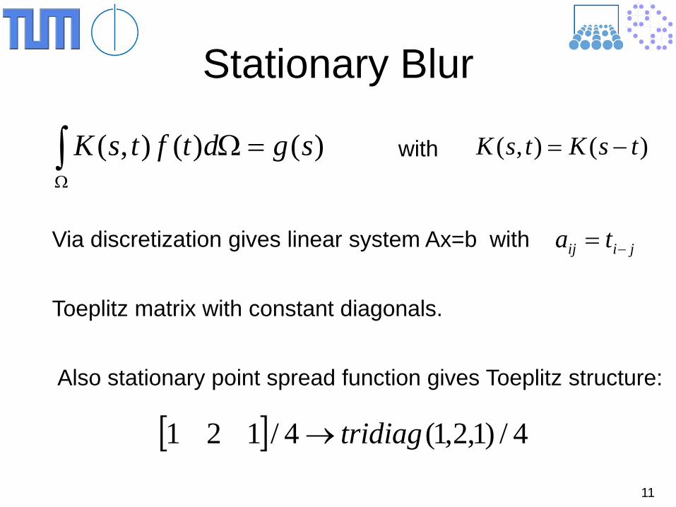
Stationary Blur

)()(),( sgdtftsK =Ω∫Ω

with )(),( tsKtsK −=

Via discretization gives linear system Ax=b with jiij ta −=

Toeplitz matrix with constant diagonals.

Also stationary point spread function gives Toeplitz structure:

[ ] 4/)1,2,1(4/121 tridiag→

−

−

−

−−

011

101

101

110

....

.....

....

tttttt

tttttt

n

n

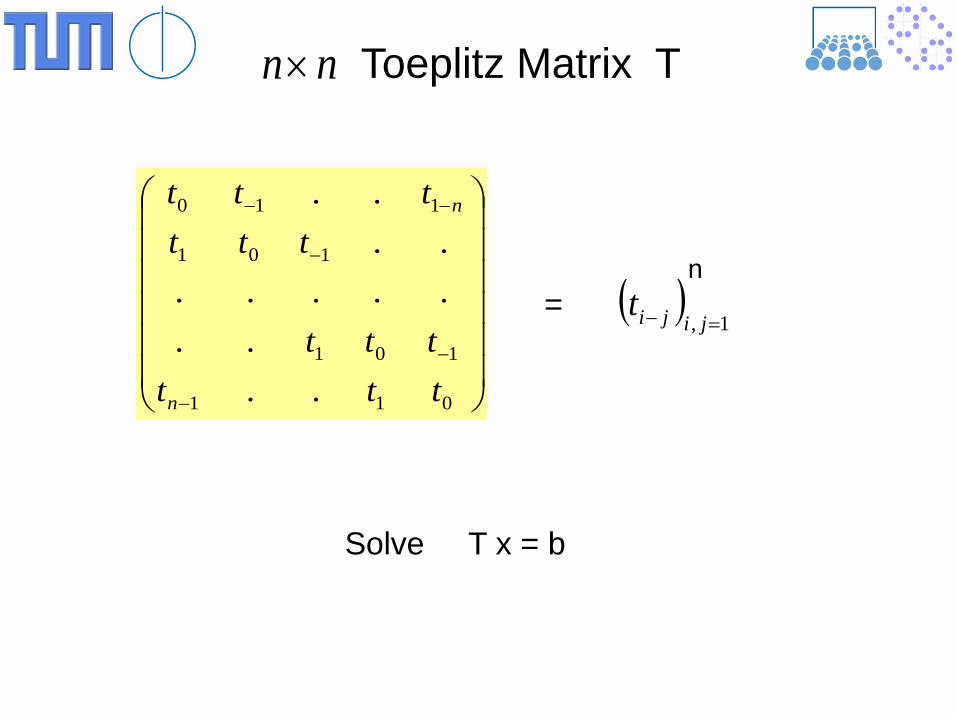
Toeplitz Matrix T nn×

Solve T x = b

( )1, =− jijit

n =

13

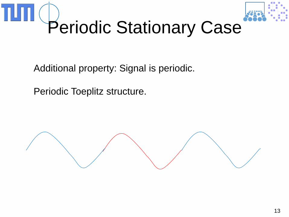
Periodic Stationary Case

Additional property: Signal is periodic. Periodic Toeplitz structure.

14

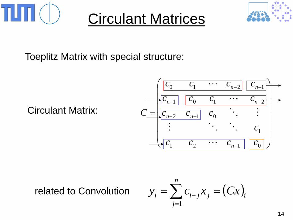
Circulant Matrices

Toeplitz Matrix with special structure:

=

−

−−

−−

−−

0121

1

012

2101

1210

ccccc

ccccccccccc

C

n

nn

nn

nn

related to Convolution ( )ij

n

jjii Cxxcy ==∑

=−

1

Circulant Matrix:

15

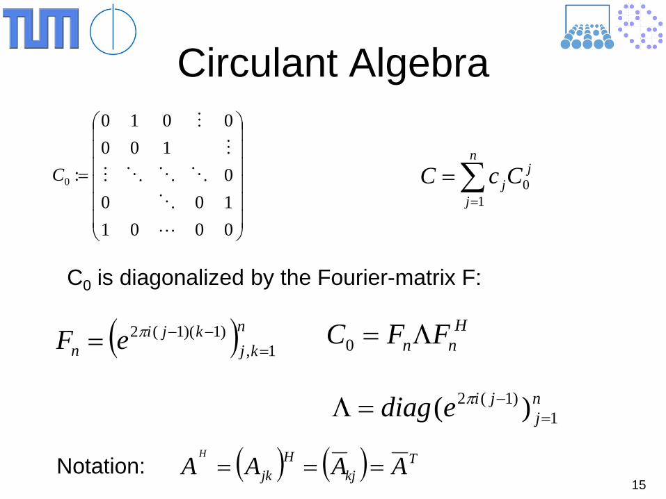
Circulant Algebra

=

00011000

1000010

:0

C ∑=

=n

j

jjCcC

10

C0 is diagonalized by the Fourier-matrix F:

( )n kjkji

n eF 1,)1)(1(2

=−−= π H

nn FFC Λ=0

nj

jiediag 1)1(2 )( =

−=Λ π

Notation: ( ) ( ) Tkj

Hjk AAAA

H

===

16

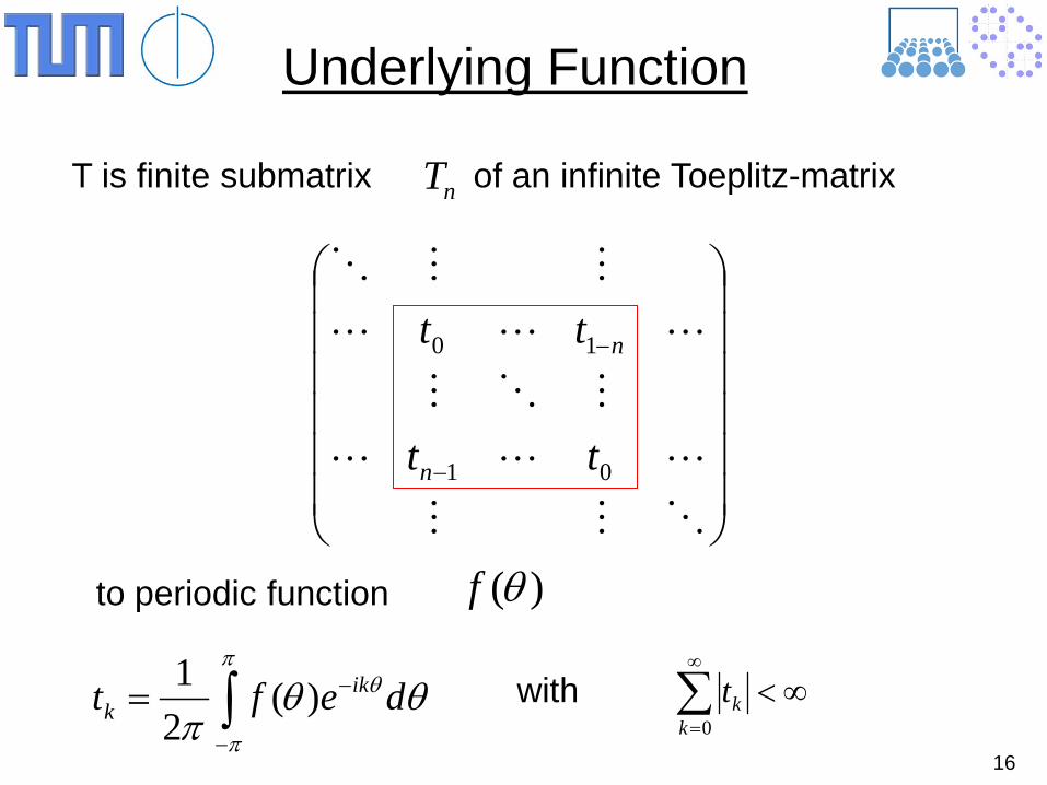
Underlying Function

T is finite submatrix of an infinite Toeplitz-matrix nT

−

−

01

10

tt

tt

n

n

to periodic function )(θf

∫−

−=π

π

θ θθπ

deft ikk )(

21 ∞<∑

∞

=0kktwith

17

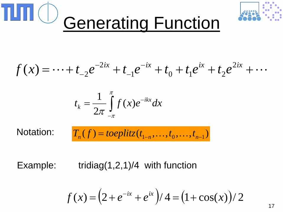
Generating Function

++++++= −−

−−

ixixixix etettetetxf 22101

22)(

∫−

−=π

ππdxexft ikx

k )(21

Example: tridiag(1,2,1)/4 with function

( ) ( ) 2/)cos(14/2)( xeexf ixix +=++= −

Notation: ),,,,()( 101 −−= nnn ttttoeplitzfT

18

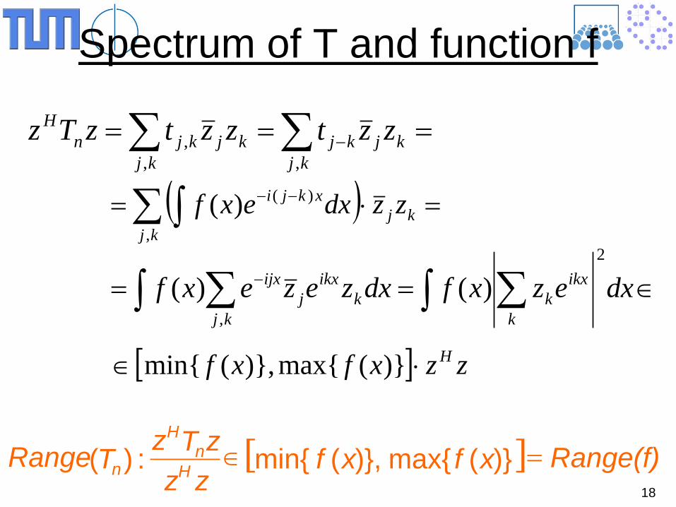
Spectrum of T and function f

=== ∑∑ − kjkj

kjkjkj

kjnH zztzztzTz

,,,

( ) =⋅=∑ ∫ −−kj

kj

xkji zzdxexf,

)()(

∈== ∫ ∑∑∫ − dxezxfdxzezexfk

ikxkk

ikxj

kj

ijx2

,)()(

[ ] zzxfxf H⋅∈ )(max),(min

[ ] ) ( max ), ( min : ) ( Range(f) x f x f z z z T z T Range H

n H

n = ∈

19

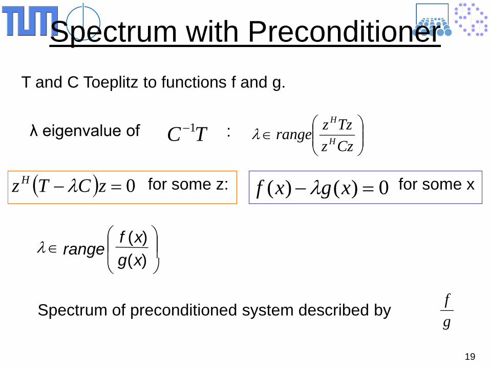
Spectrum with Preconditioner T and C Toeplitz to functions f and g.

∈

) ( ) (

x g x f

range λ

λ eigenvalue of TC 1−

∈

CzzTzzrange H

H

λ:

0)()( =− xgxf λ( ) 0=− zCTz H λ for some z:

Spectrum of preconditioned system described by gf

for some x

20

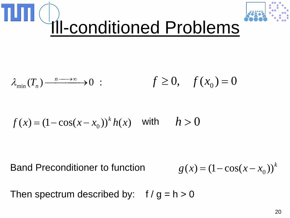
Ill-conditioned Problems

:0)(min → ∞→nnTλ 0)(,0 0 =≥ xff

Band Preconditioner to function kxxxg ))cos(1()( 0−−=

Then spectrum described by: f / g = h > 0

)())cos(1()( 0 xhxxxf k−−= 0>hwith

21

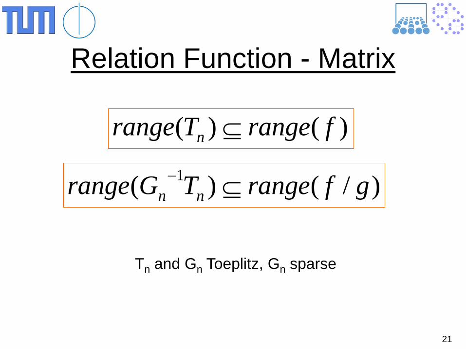
Relation Function - Matrix

)()( frangeTrange n ⊆

)/()( 1 gfrangeTGrange nn ⊆−

Tn and Gn Toeplitz, Gn sparse

22

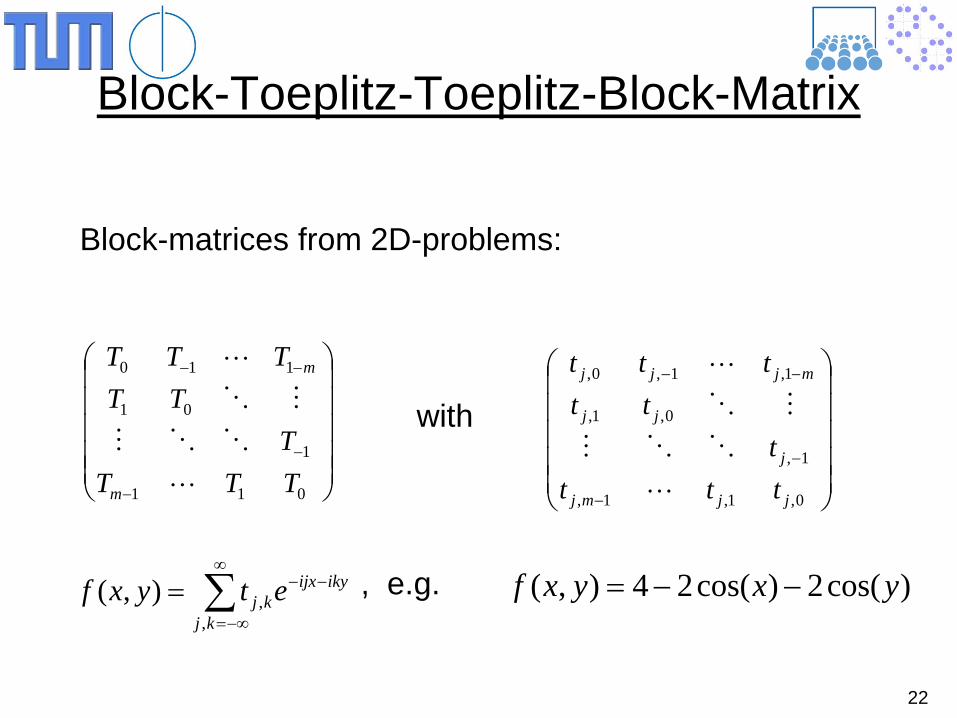
Block-Toeplitz-Toeplitz-Block-Matrix

Block-matrices from 2D-problems:

−

−

−−

011

1

01

110

TTTT

TTTTT

m

m

−

−

−−

0,1,1,

1,

0,1,

1,1,0,

jjmj

j

jj

mjjj

tttt

ttttt

with

ikyijx

kjkj etyxf −−

∞

−∞=∑=,

,),( )cos(2)cos(24),( yxyxf −−=, e.g.

23

Ill-posed Inverse Problems Further Examples

- Computer Tomography - Impedance Tomography - Supersonic Tomography - Inverse Heat Conduction

24

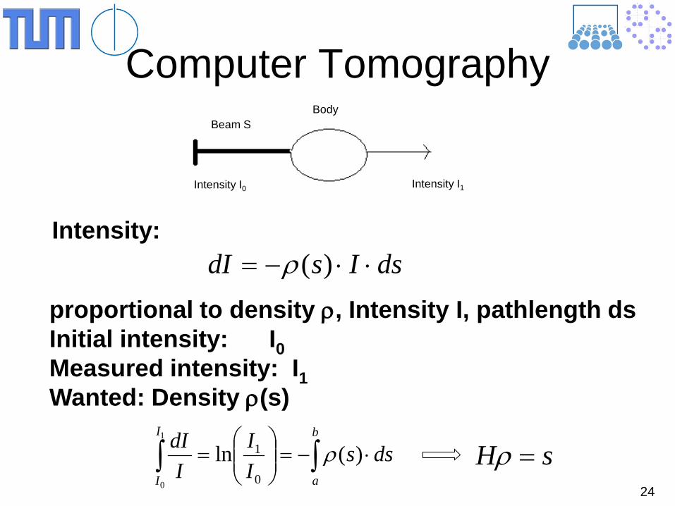
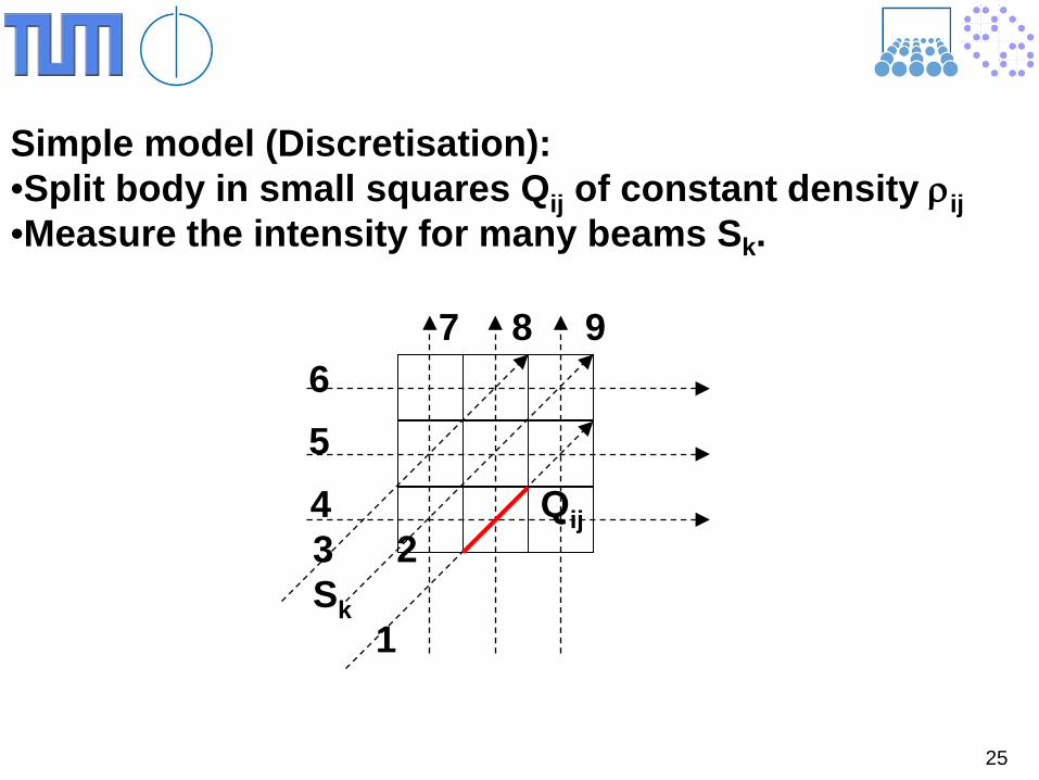
Computer Tomography

dsIsdI ⋅⋅−= )(ρ

∫∫ ⋅−=

=

b

a

I

I

dssII

IdI )(ln

0

11

0

ρ

Intensity:

proportional to density ρ, Intensity I, pathlength ds Initial intensity: I0 Measured intensity: I1 Wanted: Density ρ(s)

sH =ρ

Body Beam S

Intensity I0 Intensity I1

25

Simple model (Discretisation): •Split body in small squares Qij of constant density ρij •Measure the intensity for many beams Sk.

6 5

7 8 9

4 Qij 3 2 Sk 1

26

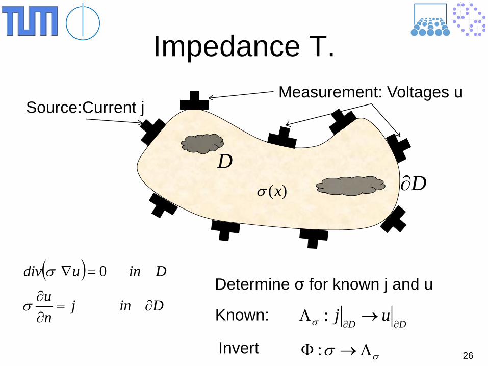
Impedance T.

Source:Current j Measurement: Voltages u

D)(xσ D∂

( )Dinj

nu

Dinudiv

∂=∂∂

=∇

σ

σ 0Determine σ for known j and u

DDuj

∂∂→Λ :σKnown:

σσ Λ→Φ :Invert

27

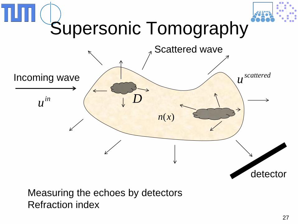
Supersonic Tomography

Incoming wave

Scattered wave

detector

inu

scattereduD

)(xn

Measuring the echoes by detectors Refraction index

28

Heat Conduction

1) Measuring the heat distribution at time T, determine the heat distribution at time t<T

2) From the heat conduction at the surface determine the heat distribution in the interior

3) Measuring the temperature on the surface, determine the thermal conductivity.

30

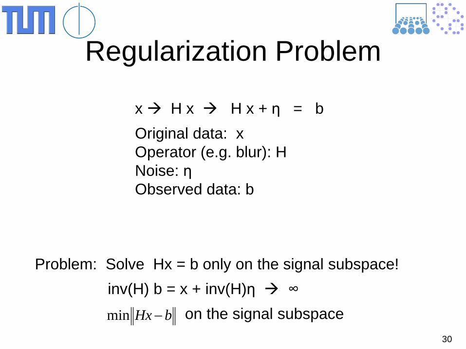
Regularization Problem

x H x H x + η = b

Original data: x Operator (e.g. blur): H Noise: η Observed data: b

Problem: Solve Hx = b only on the signal subspace!

inv(H) b = x + inv(H)η ∞

on the signal subspace bHx −min

31

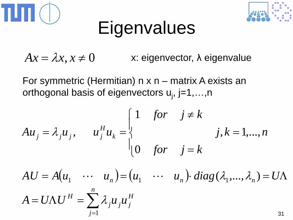
Eigenvalues 0, ≠= xxAx λ x: eigenvector, λ eigenvalue

For symmetric (Hermitian) n x n – matrix A exists an orthogonal basis of eigenvectors uj, j=1,…,n

nkjkjfor

kjforuuuAu k

Hjjjj ,...,1,

0

1, =

=

≠== λ

( ) ( ) Λ=⋅== UdiaguuuuAAU nnn ),...,( 111 λλ

∑=

=Λ=n

j

Hjjj

H uuUUA1λ

32

Computing Eigenpairs

Extreme eigenvalue: Power iteration, Lanczos, Arnoldi

Interior eigenvalues: Inverse Iteration, Jacobi Davidson, LOBPCG

All eigenpairs: Tridiagonalization + QR, Divide&Conquer, MR3,…

MATLAB: eig or eigs, LAPACK, ScaLAPACK,…

33

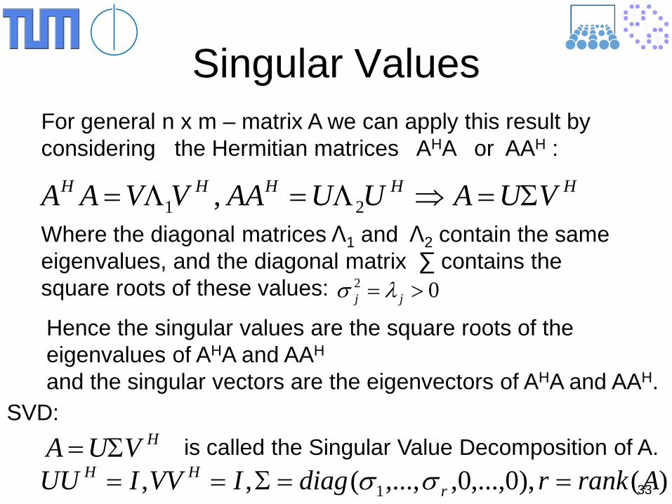
Singular Values For general n x m – matrix A we can apply this result by considering the Hermitian matrices AHA or AAH :

HHHHH VUAUUAAVVAA Σ=⇒Λ=Λ= 21 ,Where the diagonal matrices Λ1 and Λ2 contain the same eigenvalues, and the diagonal matrix ∑ contains the square roots of these values: 02 >= jj λσ

Hence the singular values are the square roots of the eigenvalues of AHA and AAH and the singular vectors are the eigenvectors of AHA and AAH.

HVUA Σ= is called the Singular Value Decomposition of A. )(),0,...,0,,...,(,, 1 ArankrdiagIVVIUU r

HH ==Σ== σσ

SVD:

34

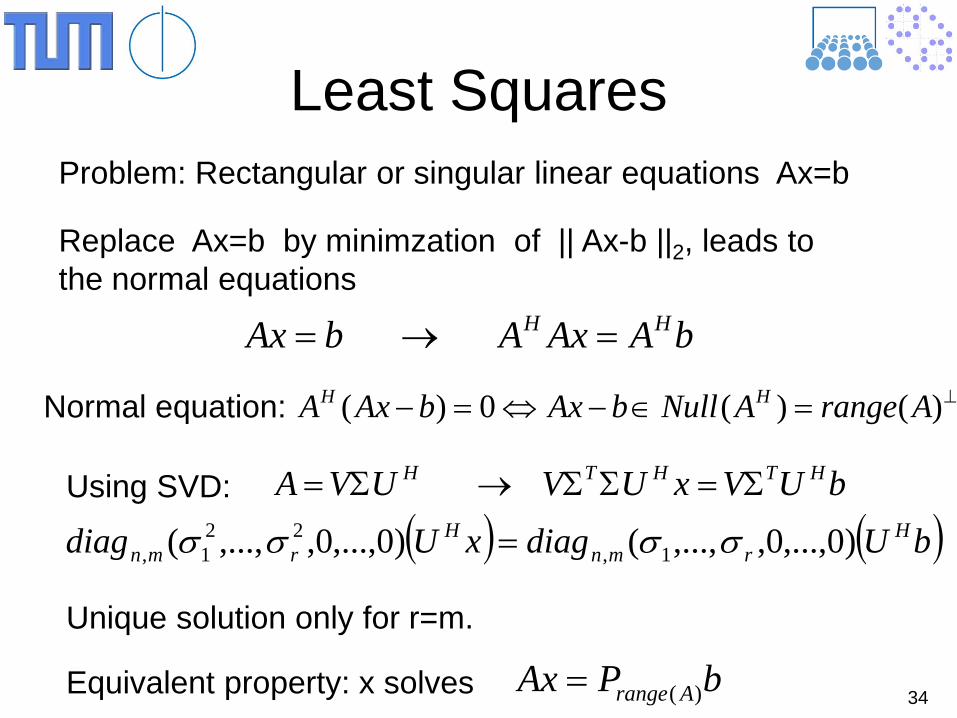
Least Squares Problem: Rectangular or singular linear equations Ax=b

Replace Ax=b by minimzation of || Ax-b ||2, leads to the normal equations

bAAxAbAx HH =→=

Using SVD: bUVxUVUVA HTHTH Σ=ΣΣ→Σ=

( ) ( )bUdiagxUdiag Hrmn

Hrmn )0,...,0,,...,()0,...,0,,...,( 1,22

1, σσσσ =

Unique solution only for r=m.

Equivalent property: x solves bPAx Arange )(=

Normal equation: ⊥=∈−⇔=− )()(0)( ArangeANullbAxbAxA HH

35

Linear Systems

Solving Ax=b: Gaussian Elimination Pivot, LU-factorization

QR-decomposition for ill-conditioned rectangular rank revealing

Regularization one step further for extremely ill-conditioned singular systems

(Iterative methods: Gauss-Seidel, Krylov)

36

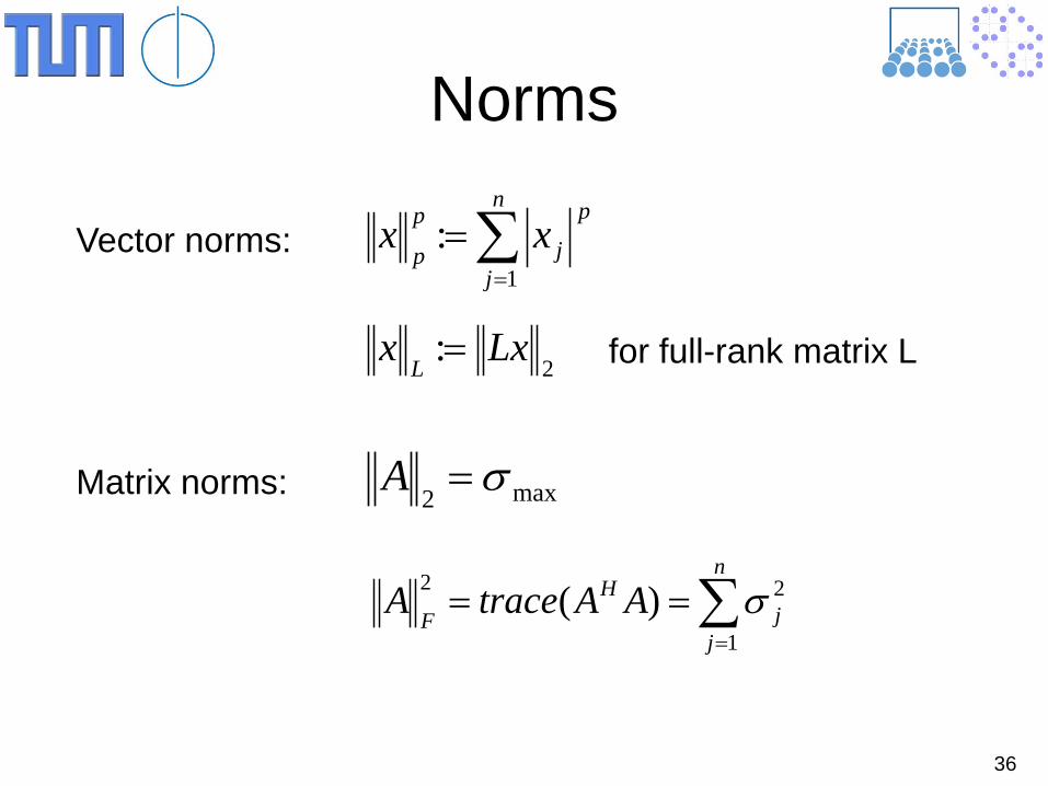
Norms

Vector norms: ∑=

=n

j

p

jp

pxx

1:

2: Lxx

L= for full-rank matrix L

Matrix norms: max2σ=A

∑=

==n

jj

HF

AAtraceA1

22 )( σ

37

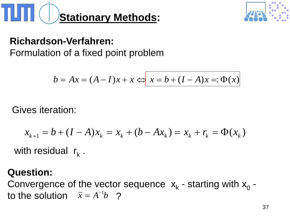
)(:)()( xxAIbxxxIAAxb Φ=−+=⇔+−==

Stationary Methods: Richardson-Verfahren: Formulation of a fixed point problem

Question: Convergence of the vector sequence xk - starting with x0 - to the solution bAx 1−= ?

)()()(1 kkkkkkk xrxAxbxxAIbx Φ=+=−+=−+=+

Gives iteration:

with residual rk .

38

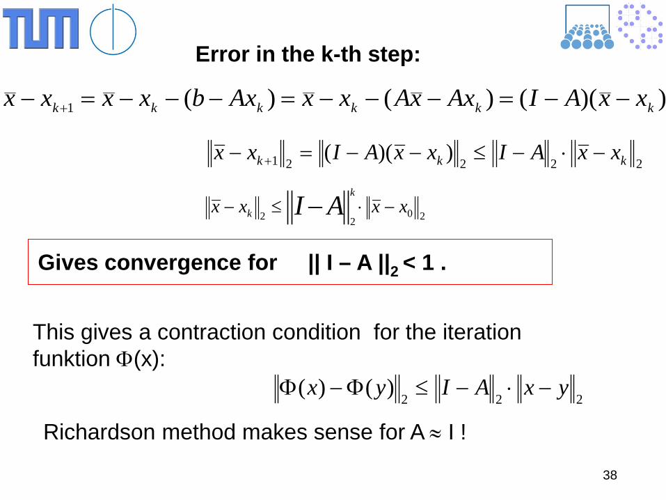
))(()()(1 kkkkkk xxAIAxxAxxAxbxxxx −−=−−−=−−−=− +

22221 ))(( kkk xxAIxxAIxx −⋅−≤−−=− +

2022

xxxx AIk

k −⋅≤− −

Error in the k-th step:

Gives convergence for || I – A ||2 < 1 .

222)()( yxAIyx −⋅−≤Φ−Φ

Richardson method makes sense for A ≈ I !

This gives a contraction condition for the iteration funktion Φ(x):

39

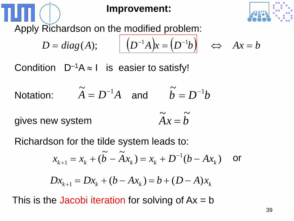
( ) ( ) bAxbDxADAdiagD =⇔== −− 11);(

Improvement:

Apply Richardson on the modified problem:

Condition D–1A ≈ I is easier to satisfy!

)()~~( 11 kkkkk AxbDxxAbxx −+=−+= −+

kkkk xADbAxbDxDx )()(1 −+=−+=+

Richardson for the tilde system leads to:

or

This is the Jacobi iteration for solving of Ax = b

ADA 1~ −= bDb 1~ −=

bxA ~~=

and

gives new system

Notation:

40

12

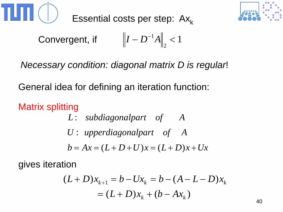
1 <− − ADI

Essential costs per step: Axk

Necessary condition: diagonal matrix D is regular!

UxxDLxUDLAxbAofnalpartupperdiagoUAoflpartsubdiagonaL

++=++== )()(

::

)()()()( 1

kk

kkk

AxbxDLxDLAbUxbxDL

−++=−−−=−=+ +

gives iteration

Matrix splitting

General idea for defining an iteration function:

Convergent, if

41

( ) k

kkk

xADLIbDLAxbDLxx

11

11

)()(

)()(−−

−+

+−++=

−++=

1)(2

1 <+− − ADLI

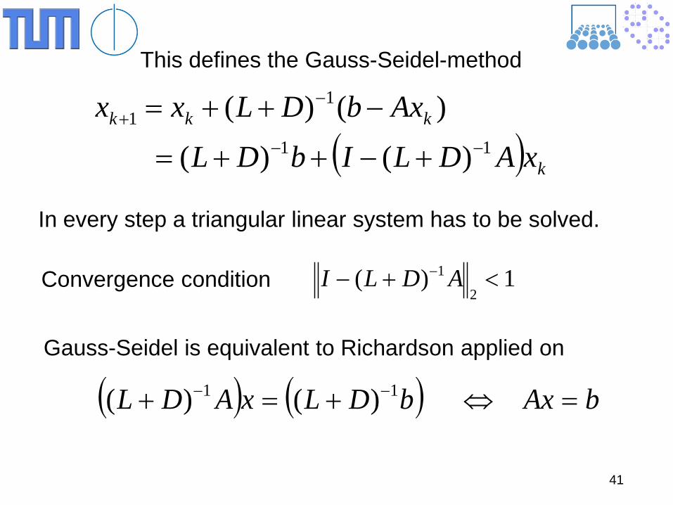
This defines the Gauss-Seidel-method

In every step a triangular linear system has to be solved.

( ) ( ) bAxbDLxADL =⇔+=+ −− 11 )()(

Gauss-Seidel is equivalent to Richardson applied on

Convergence condition

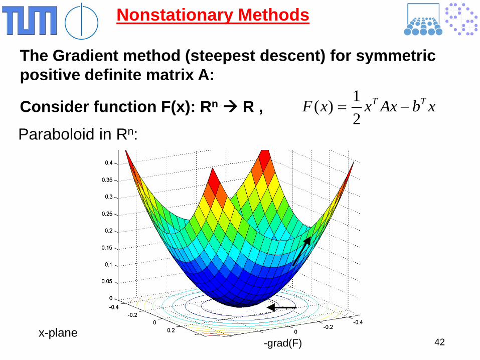
Nonstationary Methods The Gradient method (steepest descent) for symmetric positive definite matrix A: Consider function F(x): Rn R ,

42

xbAxxxF TT −=21)(

Paraboloid in Rn:

-grad(F) x-plane

43

bAxbAxxF =⇔=−=∇ 0)(

Minimum of this function is the point with horizontal tangent vector = the position with gradient zero:

x where the paraboloid takes its minimum is exactly the solution of the linear system!

Consider minimization! From actual position xk the next iterate xk+1 should be chosen in such a way, that it is closer to the minimum. xk+1 = xk + αkdk Search direction dk and stepsize αk. Find search direction, such that the function gets smaller:

Directional derivate in direction n is given by , and takes its maximum absolute value for .

Therefore, is locally the direction of the steepest descent towards the minimum.

44

nF ⋅∇Fn ∇=2F∇

Fn −∇=

Descent direction is given by the negative gradient!

)()(1 kkkkkkk AxbxxFxx −+=∇−=+ αα

Hence, the function values get smaller moving in this descent direction

Choose

It remains to determine the optimal stepsize αk, that leads as close as possible to the minimum!

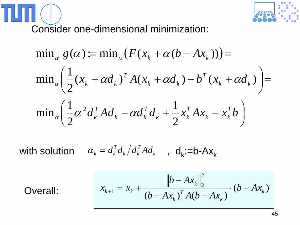
45

( )

−+−

=

+−++

=−+=

bxAxxddAdd

dxbdxAdx

AxbxFg

Tkk

Tkk

Tkk

Tk

kkT

kkT

kk

kk

21

21min

)()()(21min

))((min:)(min

2 αα

ααα

αα

α

α

αα

kTkk

Tkk Adddd=α

Consider one-dimensional minimization:

with solution , dk:=b-Axk

)()()(

2

21 k

kT

k

kkk Axb

AxbAAxbAxb

xx −⋅−−

−+=+Overall:

46

Method of steepest descent or gradient method. Disadvantage: In case of strongly distorted paraboloid: Very slow convergence.

47

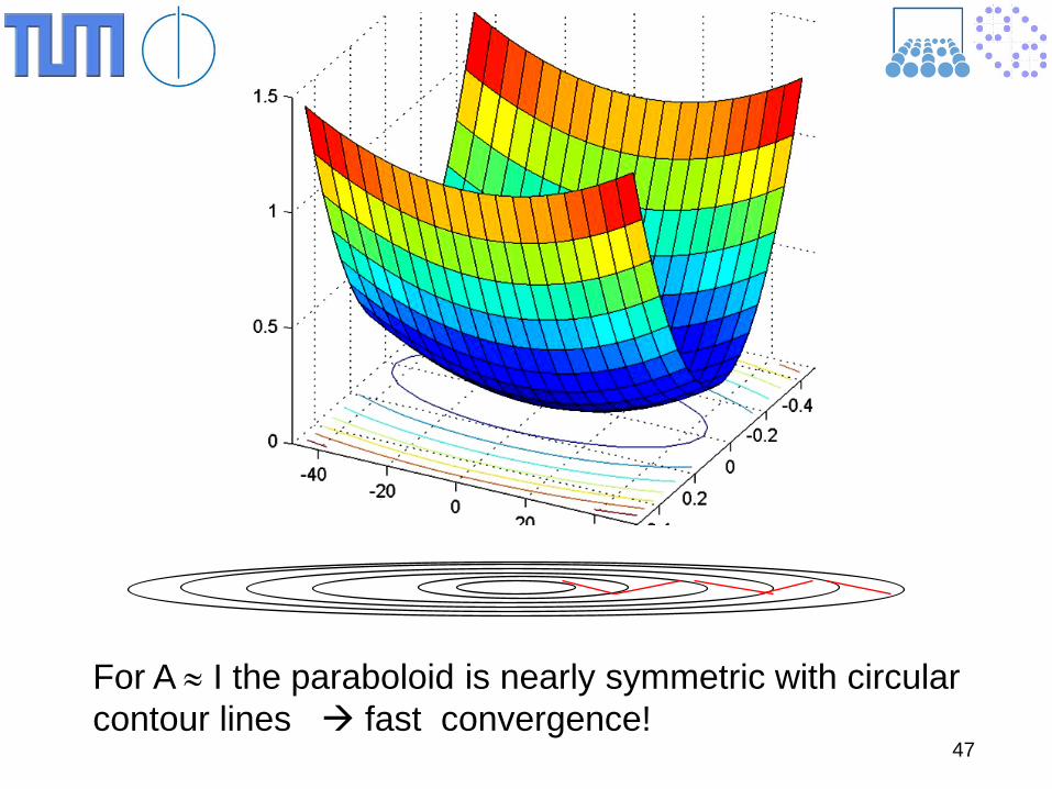
For A ≈ I the paraboloid is nearly symmetric with circular contour lines fast convergence!

48

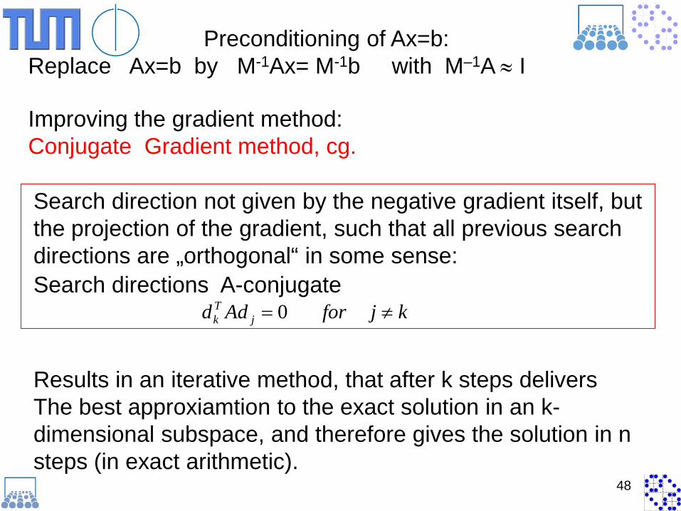
Preconditioning of Ax=b: Replace Ax=b by M-1Ax= M-1b with M–1A ≈ I

kjforAdd jTk ≠= 0

Search direction not given by the negative gradient itself, but the projection of the gradient, such that all previous search directions are „orthogonal“ in some sense: Search directions A-conjugate

Results in an iterative method, that after k steps delivers The best approxiamtion to the exact solution in an k-dimensional subspace, and therefore gives the solution in n steps (in exact arithmetic).

Improving the gradient method: Conjugate Gradient method, cg.

49

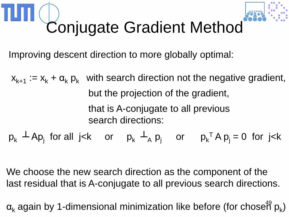
Conjugate Gradient Method

Improving descent direction to more globally optimal: xk+1 := xk + αk pk with search direction not the negative gradient,

but the projection of the gradient,

that is A-conjugate to all previous search directions:

pk Apj for all j<k or pk A pj or pkT A pj = 0 for j<k

We choose the new search direction as the component of the last residual that is A-conjugate to all previous search directions. αk again by 1-dimensional minimization like before (for chosen pk)

50

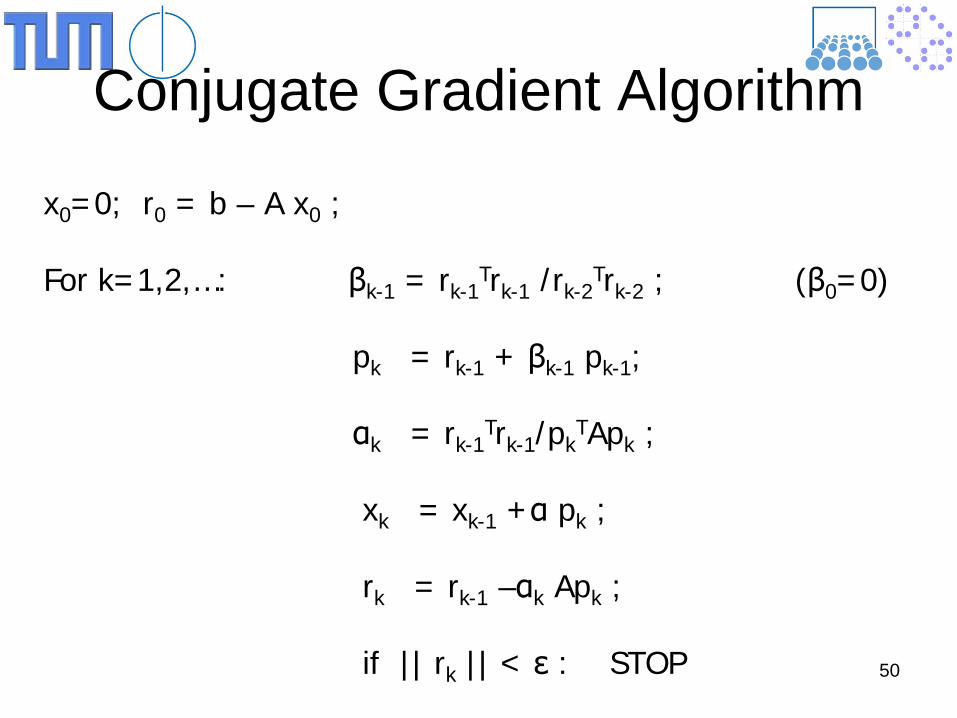
Conjugate Gradient Algorithm

x0=0; r0 = b – A x0 ; For k=1,2,…: βk-1 = rk-1

Trk-1 /rk-2Trk-2 ; (β0=0)

pk = rk-1 + βk-1 pk-1; αk = rk-1

Trk-1/pkTApk ;

xk = xk-1 +α pk ; rk = rk-1 –αk Apk ; if || rk || < ε : STOP

51

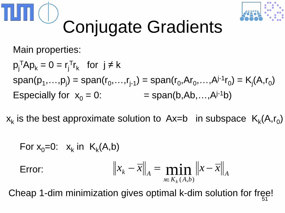
Conjugate Gradients

Main properties:

pjTApk = 0 = rj

Trk for j ≠ k

span(p1,…,pj) = span(r0,…,rj-1) = span(r0,Ar0,…,Aj-1r0) = Kj(A,r0)

Especially for x0 = 0: = span(b,Ab,…,Aj-1b)

xk is the best approximate solution to Ax=b in subspace Kk(A,r0)

AbAKx

Ak xxxxk

−=−∈min

),(

For x0=0: xk in Kk(A,b) Error:

Cheap 1-dim minimization gives optimal k-dim solution for free!

52

Conjugate Gradients

Consequence: After n steps Kn(A,b) = Rn and therefore

xn = A-1 b is the solution in exact arithmetic. Unfortunately this is not true in floating point arithmetic. Furthermore, also O(n) iteration steps would be too costly: costs: #iterations * matrix-vector-product Matrix-vector-product easy in parallel. But, how to get fast convergence and reduce the number of iterations?

53

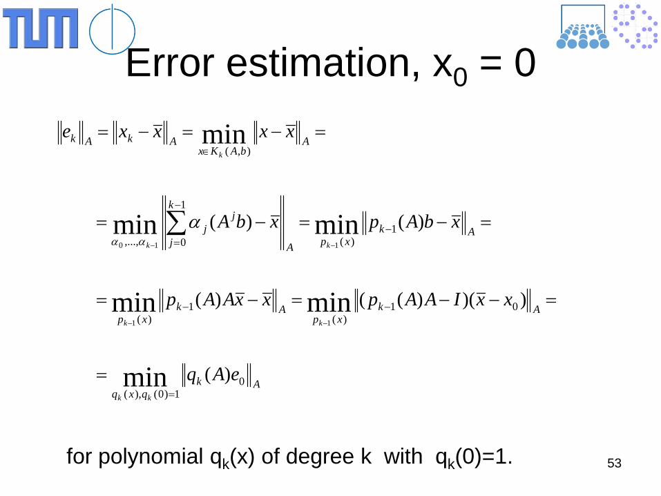
Error estimation, x0 = 0

Akqxq

Akxp

Akxp

AkxpA

k

j

jj

AbAKx

AkAk

eAq

xxIAApxxAAp

xbApxbA

xxxxe

kk

kk

kk

k

01)0(),(

01)(

1)(

1)(

1

0,...,

),(

)(

))()(()(

)()(

min

minmin

minmin

min

11

110

=

−−

−

−

=

∈

=

=−−=−=

=−=−=

=−=−=

−−

−−

∑ααα

for polynomial qk(x) of degree k with qk(0)=1.

54

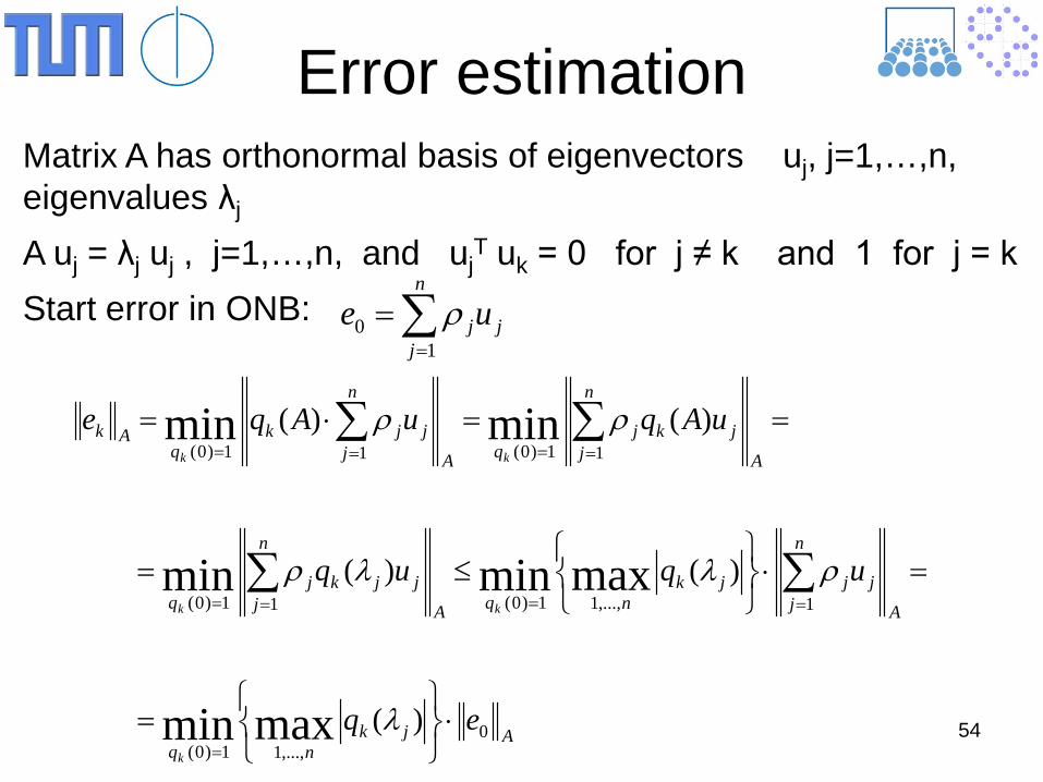
Error estimation

∑=

=n

jjjue

10 ρ

Matrix A has orthonormal basis of eigenvectors uj, j=1,…,n, eigenvalues λj

A uj = λj uj , j=1,…,n, and ujT uk = 0 for j ≠ k and 1 for j = k

Start error in ONB:

Ajknq

A

n

jjjjk

nqA

n

jjjkj

q

A

n

jjkj

qA

n

jjjk

qAk

eq

uquq

uAquAqe

k

kk

kk

0,...,11)0(

1,...,11)0(11)0(

11)0(11)0(

)(

)()(

)()(

maxmin

maxminmin

minmin

⋅

=

=⋅

≤=

==⋅=

=

====

====

∑∑

∑∑

λ

ρλλρ

ρρ

55

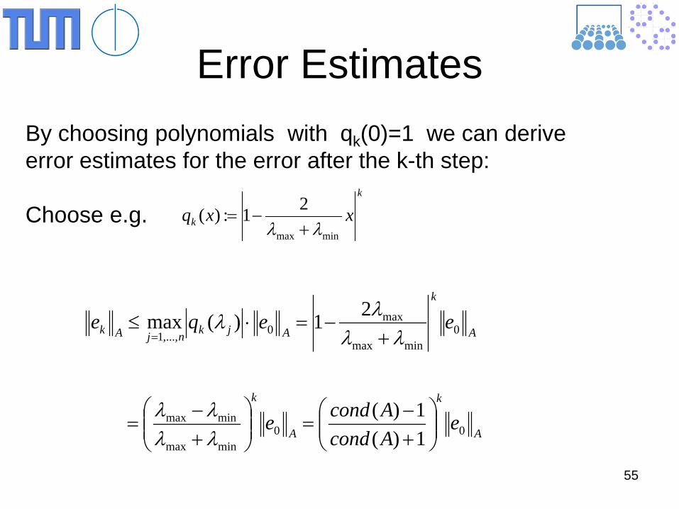
Error Estimates

k

k xxqminmax

21:)(λλ +

−=

By choosing polynomials with qk(0)=1 we can derive error estimates for the error after the k-th step: Choose e.g.

A

k

A

k

A

k

AjknjAk

eAcondAconde

eeqe

00minmax

minmax

0minmax

max0,...,1

1)(1)(

21)(max

+−

=

+−

=

+−=⋅≤

=

λλλλ

λλλλ

56

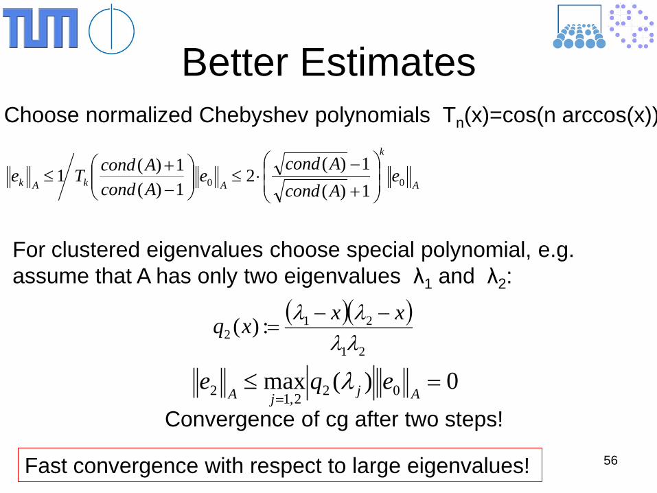
Better Estimates

A

k

AkAk eAcondAcond

eAcondAcondTe 00 1)(

1)(2

1)(1)(1

+−

⋅≤

−+

≤

Choose normalized Chebyshev polynomials Tn(x)=cos(n arccos(x))

For clustered eigenvalues choose special polynomial, e.g. assume that A has only two eigenvalues λ1 and λ2:

( )( )21

212 :)(

λλλλ xxxq −−

=

0)(max 022,12 =≤= AjjA

eqe λConvergence of cg after two steps!

Fast convergence with respect to large eigenvalues!

57

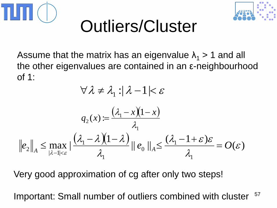
Outliers/Cluster

Assume that the matrix has an eigenvalue λ1 > 1 and all the other eigenvalues are contained in an ε-neighbourhood of 1:

( )( )1

12

1:)(λ

λ xxxq −−=

( )( ) )()1(||||1|max1

10

1

1

|1|2 ελ

εελλ

λλλελ

Oee AA=

+−≤

−−≤

<−

Very good approximation of cg after only two steps! Important: Small number of outliers combined with cluster

ελλλ <−≠∀ |1:|1

58

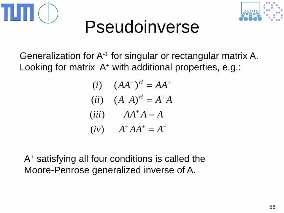
Pseudoinverse Generalization for A-1 for singular or rectangular matrix A. Looking for matrix A+ with additional properties, e.g.:

+++

+

++

++

====

AAAAivAAAAiii

AAAAiiAAAAi

H

H

)()(

)()()()(

A+ satisfying all four conditions is called the Moore-Penrose generalized inverse of A.

59

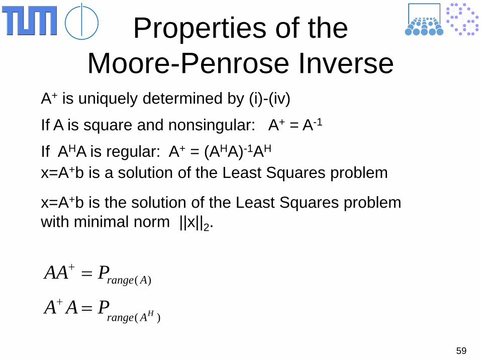
Properties of the Moore-Penrose Inverse

If A is square and nonsingular: A+ = A-1 A+ is uniquely determined by (i)-(iv)

x=A+b is a solution of the Least Squares problem

x=A+b is the solution of the Least Squares problem with minimal norm ||x||2.

If AHA is regular: A+ = (AHA)-1AH

)(

)(

HArange

Arange

PAA

PAA

=

=+

+

60

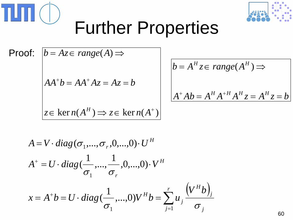
Further Properties

H

r

Hr

VdiagUA

UdiagVA

⋅⋅=

⋅⋅=

+ )0,...,0,1,...,1(

)0,...,0,,...,(

1

1

σσ

σσ

( )∑=

+ =⋅==r

j j

jH

jH bV

ubVdiagUbAx11

)0,...,1(σσ

Proof:

)(ker)(ker

)(

+

++

∈⇒∈

===

⇒∈=

AnzAnz

bAzAzAAbAA

ArangeAzb

H

bzAzAAAAbA

ArangezAb

HHHH

HH

===

⇒∈=

++

)(

61

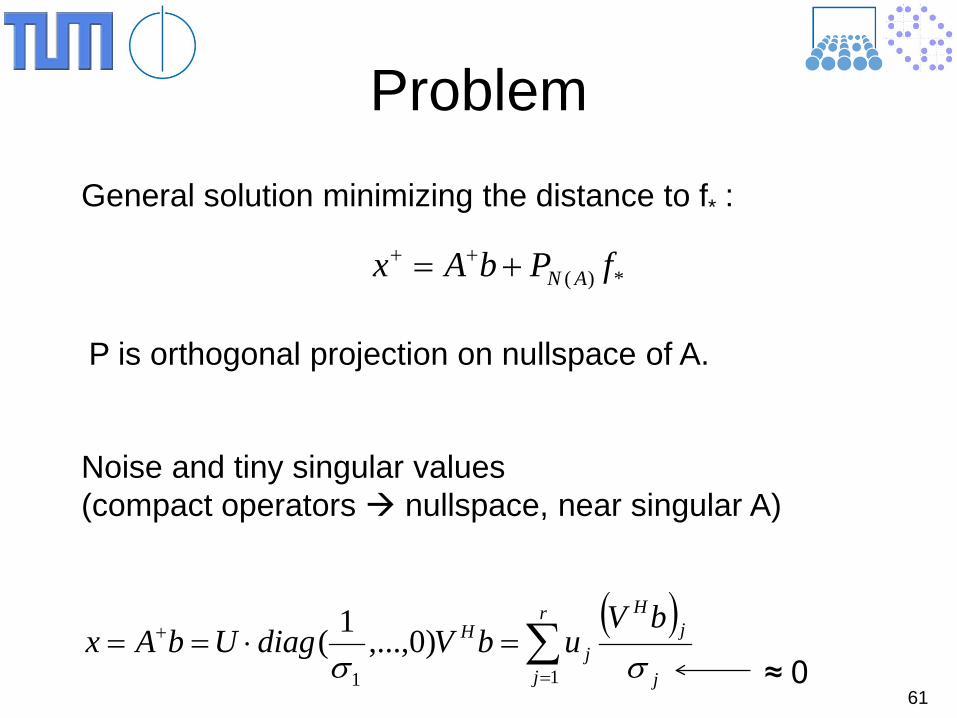
Problem General solution minimizing the distance to f* :

*)( fPbAx AN+= ++

P is orthogonal projection on nullspace of A.

Noise and tiny singular values (compact operators nullspace, near singular A)

( )∑=

+ =⋅==r

j j

jH

jH bV

ubVdiagUbAx11

)0,...,1(σσ ≈ 0

62

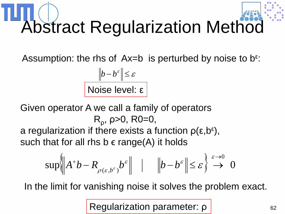
Abstract Regularization Method

Given operator A we call a family of operators Rρ, ρ>0, R0=0, a regularization if there exists a function ρ(ε,bε), such that for all rhs b ϵ range(A) it holds

0sup0

),(

→+ →≤−−

εεε

ερεε bbbRbA b

Assumption: the rhs of Ax=b is perturbed by noise to bε: εε ≤−bb

Noise level: ε

In the limit for vanishing noise it solves the problem exact.

Regularization parameter: ρ

63

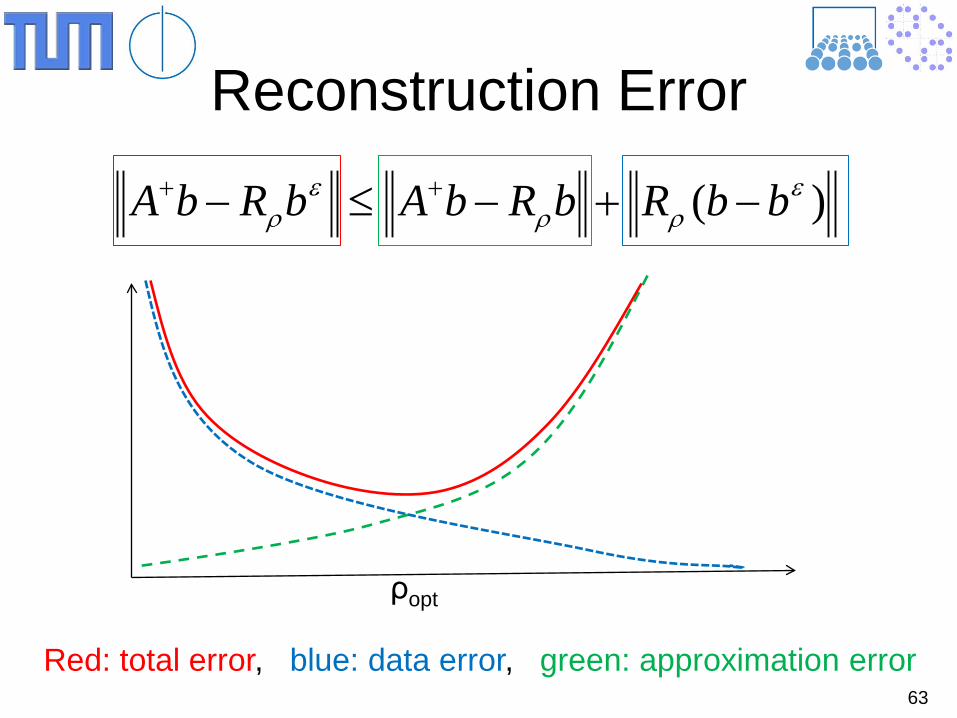
Reconstruction Error

)( ερρ

ερ bbRbRbAbRbA −+−≤− ++

Red: total error, blue: data error, green: approximation error

ρopt

64

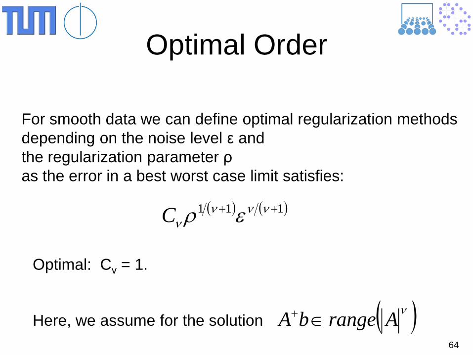
Optimal Order

For smooth data we can define optimal regularization methods depending on the noise level ε and the regularization parameter ρ as the error in a best worst case limit satisfies:

( ) ( )111 ++ νννν ερC

Optimal: Cν = 1.

Here, we assume for the solution ( )νArangebA ∈+

65

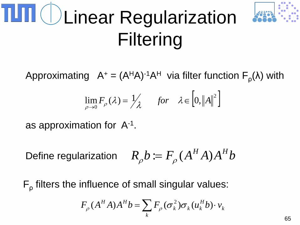
Linear Regularization Filtering

Approximating A+ = (AHA)-1AH via filter function Fρ(λ) with

[ ]2

0,01)(lim AforF ∈=

→λλλρρ

bAAAFbR HH )(: ρρ =Define regularization

as approximation for A-1.

Fρ filters the influence of small singular values:

kHkk

kk

HH vbuFbAAAF ⋅= ∑ )()()( 2 σσρρ

66

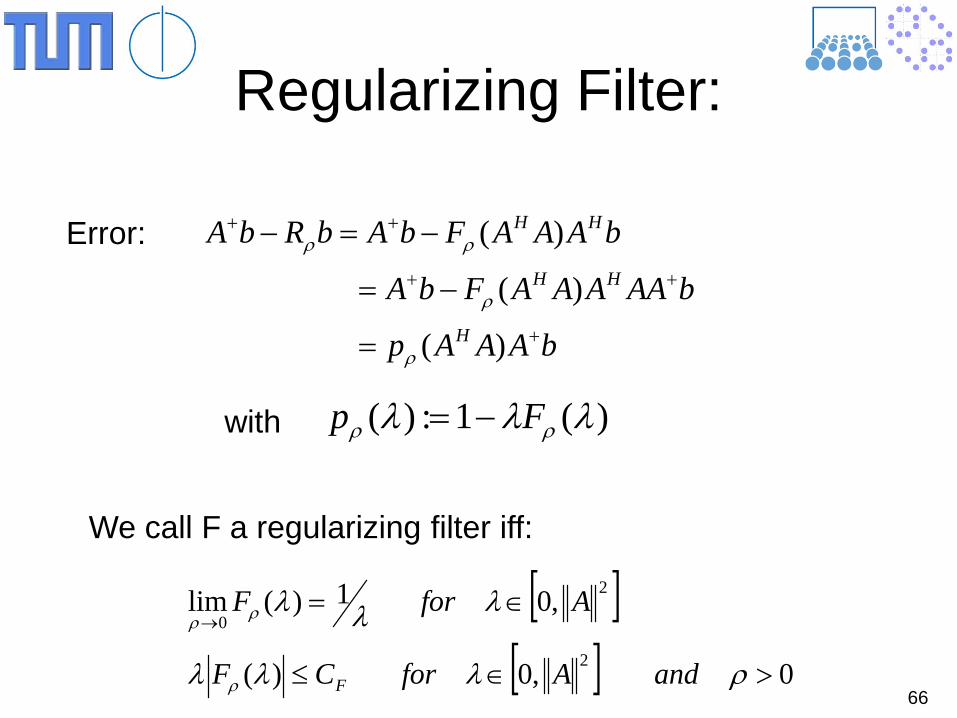
Regularizing Filter:

Error:

bAAAp

bAAAAAFbA

bAAAFbAbRbA

H

HH

HH

+

++

++

=

−=

−=−

)(

)(

)(

ρ

ρ

ρρ

)(1:)( λλλ ρρ Fp −=with

We call F a regularizing filter iff:

[ ][ ] 0,0)(

,01)(lim

2

2

0

>∈≤

∈=→

ρλλλ

λλλ

ρ

ρρ

andAforCF

AforF

F

67

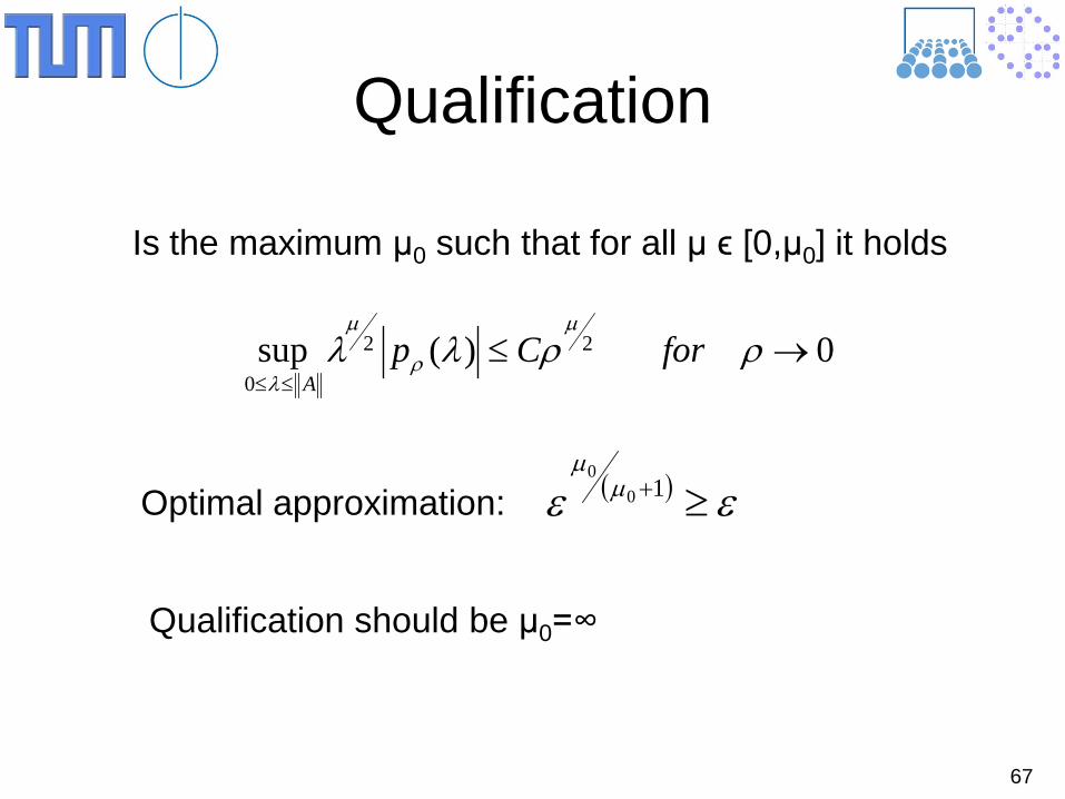
Qualification

Is the maximum μ0 such that for all μ ϵ [0,μ0] it holds

0)(sup 22

0→≤

≤≤ρρλλ

µ

ρ

µ

λforCp

A

Optimal approximation: ( ) εε µµ

≥+100

Qualification should be μ0=∞

68

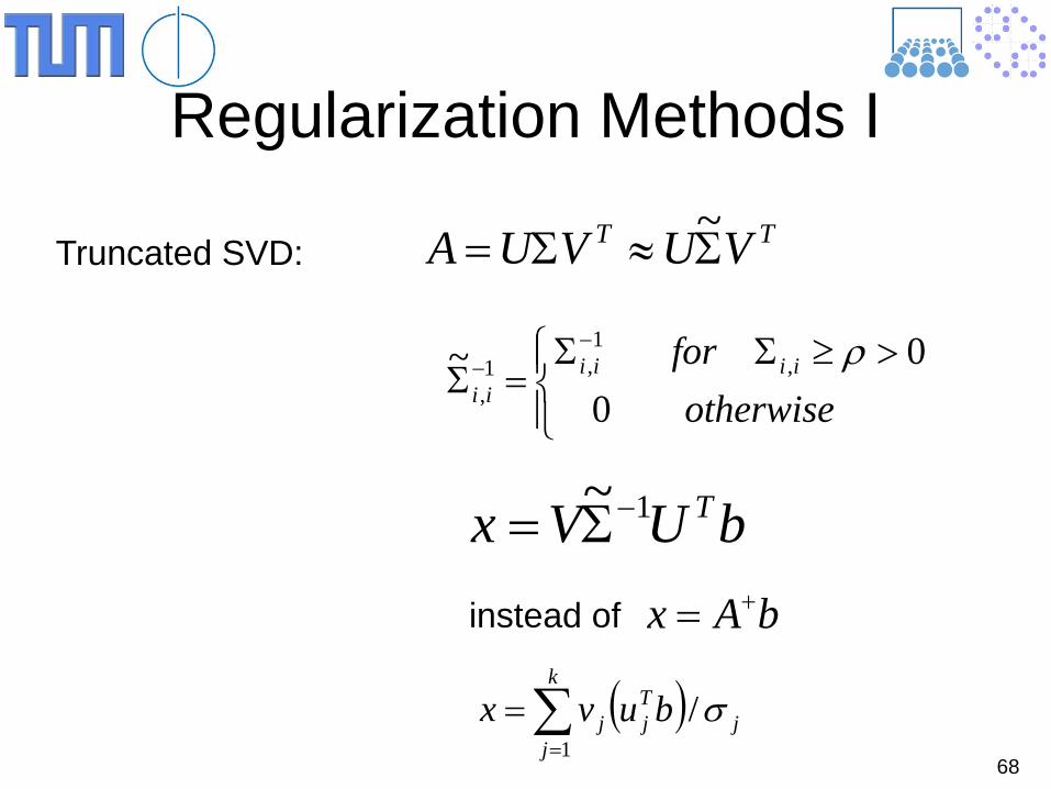
Regularization Methods I

Truncated SVD: TT VUVUA Σ≈Σ= ~

>≥ΣΣ

=Σ−

−

otherwisefor iiii

ii 00~ ,

1,1

,

ρ

bAx +=

bUVx T1~−Σ=

instead of

( )∑=

=k

jj

Tjj buvx

1/σ

69

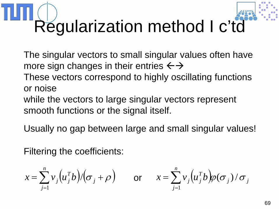
Regularization method I c’td The singular vectors to small singular values often have more sign changes in their entries These vectors correspond to highly oscillating functions or noise while the vectors to large singular vectors represent smooth functions or the signal itself.

Usually no gap between large and small singular values!

Filtering the coefficients:

( ) ( )∑=

+=n

jj

Tjj buvx

1/ ρσ ( )∑

=

=n

jjj

Tjj buvx

1/)( σσϕor

70

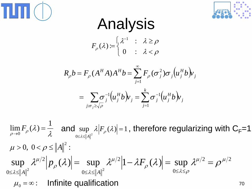
Analysis

<≥

=−

ρλρλλ

λρ :0:

:)(1

F

( )

( ) ( )∑∑

∑

=

−

≥

−

∞

=

==

==

k

jj

Hjj

jj

Hjj

jj

Hjjj

HH

vbuvbu

vbuFbAAAFbR

j 1

1

:

1

1

2 )()(

σσ

σσ

ρσ

ρρρ

λλρρ

1)(lim0

=→

F 1)(sup20

=≤≤

λλ ρλ

FA

and , therefore regularizing with CF=1

:0,0 2A≤<> ρµ22

0

2

0

2

0sup)(1sup)(sup

22

µµ

ρλρ

µ

λρ

µ

λρλλλλλλ ==−=

≤≤≤≤≤≤

FpAA

:0 ∞=µ Infinite qualification

71

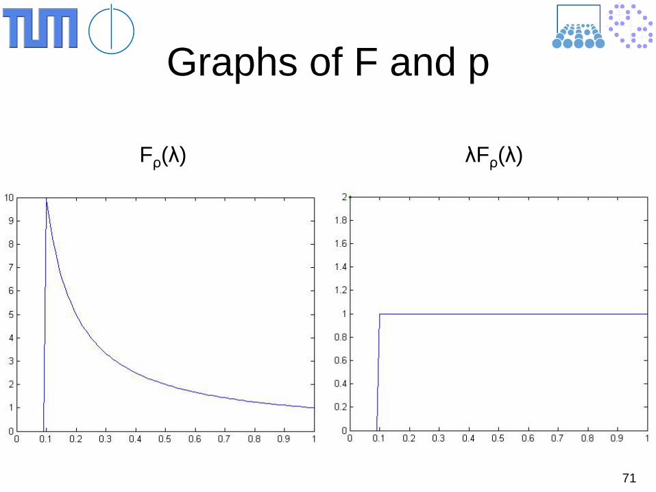
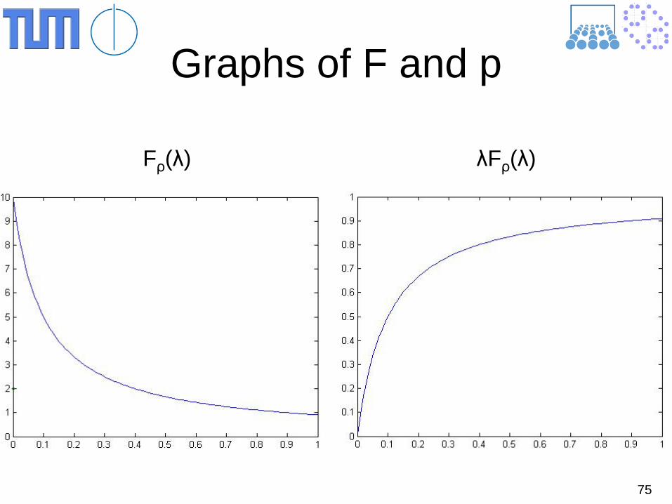
Graphs of F and p

Fρ(λ) λFρ(λ)

72

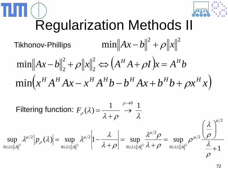
Regularization Methods II Tikhonov-Phillips

22min xbAx ρ+−

( ) bAxIAAxbAx HH =+⇔+− ρρ 2

2

2

2min

( )xxbbAxbbAxAxAx HHHHHHH ρ++−−min

Filtering function: λρλ

λρ

ρ11)(

0→

→+

=F

1supsup1sup)(sup

2

2

0

2

0

2

0

2

0 2222+

=+

=+

−=≤≤≤≤≤≤≤≤

ρλρλ

ρρλρλ

ρλλλλλ

µ

µ

λ

µ

λ

µ

λρ

µ

λ AAAAp

73

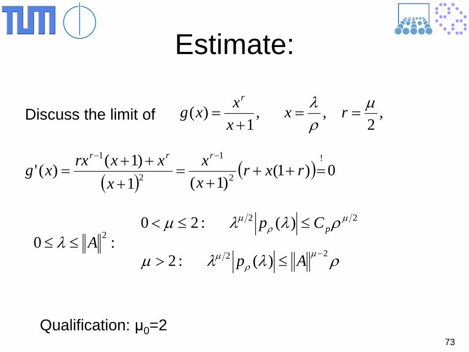
Estimate:

,2

,,1

)( µρλ

==+

= rxxxxg

r

Discuss the limit of

( )( ) 0)1(

)1(1)1()('

!

2

1

2

1

=+++

=+

++=

−−

rxrxx

xxxrxxg

rrr

22 )(:20 µρ

µ ρλλµ pCp ≤≤<

ρλλµ µρ

µ 22 )(:2 −≤> Ap:0 2A≤≤ λ

Qualification: μ0=2

74

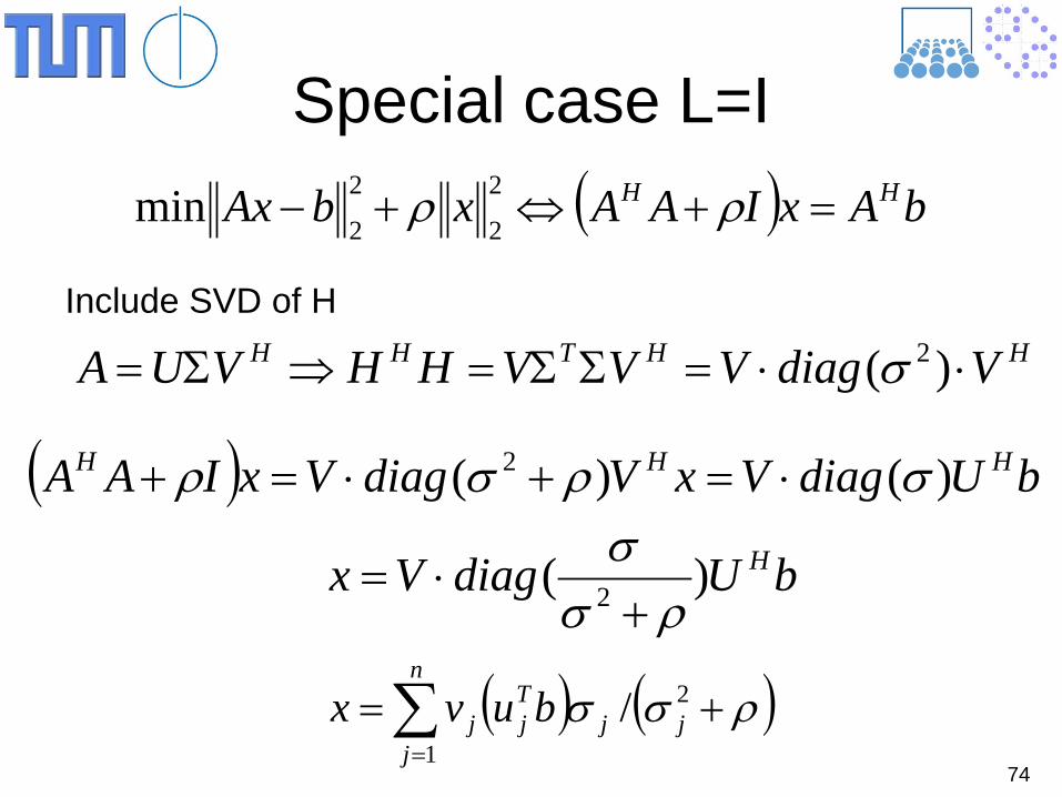
Special case L=I ( ) bAxIAAxbAx HH =+⇔+− ρρ 2

2

2

2min

Include SVD of H HHTHH VdiagVVVHHVUA ⋅⋅=ΣΣ=⇒Σ= )( 2σ

( ) bUdiagVxVdiagVxIAA HHH )()( 2 σρσρ ⋅=+⋅=+

bUdiagVx H)( 2 ρσσ+

⋅=

( ) ( )∑=

+=n

jjj

Tjj buvx

1

2/ ρσσ

75

Graphs of F and p

Fρ(λ) λFρ(λ)

76

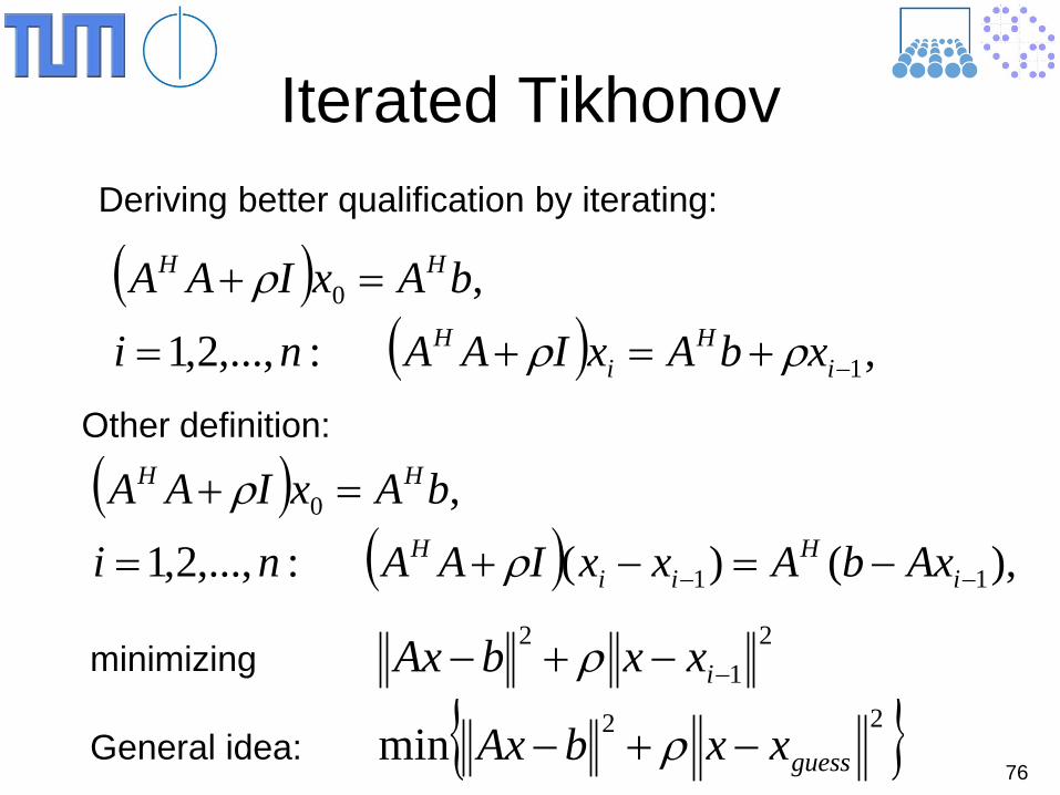
Iterated Tikhonov Deriving better qualification by iterating:

( )( ) ,:,...,2,1

,

1

0

−+=+=

=+

iH

iH

HH

xbAxIAAnibAxIAA

ρρ

ρ

Other definition:

( )( ) ),()(:,...,2,1

,

11

0

−− −=−+=

=+

iH

iiH

HH

AxbAxxIAAnibAxIAA

ρ

ρ

minimizing 2

12

−−+− ixxbAx ρ

General idea: 22min guessxxbAx −+− ρ

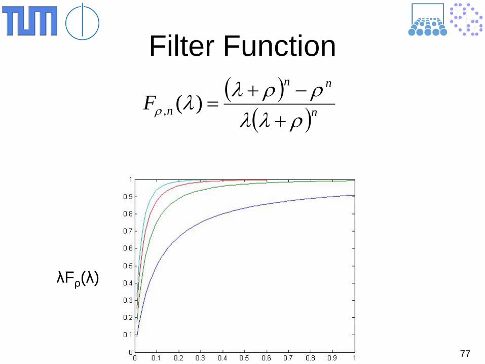
77

Filter Function ( )

( )nnn

nFρλλρρλλρ +

−+=)(,

λFρ(λ)

78

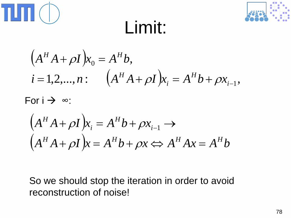
Limit: ( )

( ) ,:,...,2,1

,

1

0

−+=+=

=+

iH

iH

HH

xbAxIAAnibAxIAA

ρρ

ρ

For i ∞:

( )( ) bAAxAxbAxIAA

xbAxIAAHHHH

iH

iH

=⇔+=+

→+=+ −

ρρ

ρρ 1

So we should stop the iteration in order to avoid reconstruction of noise!

79

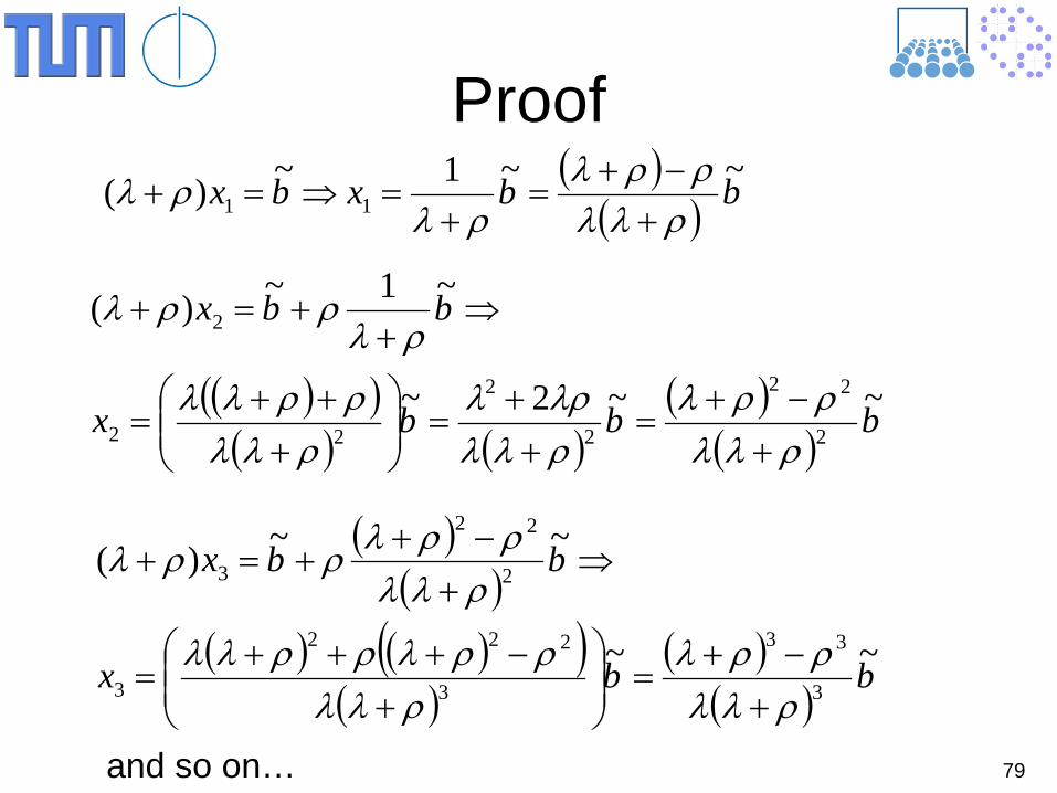
Proof ( )

( ) bbxbx ~~1~)( 11 ρλλρρλ

ρλρλ

+−+

=+

=⇒=+

( )( )( ) ( )

( )( )

bbbx

bbx

~~2~

~1~)(

2

22

2

2

22

2

ρλλρρλ

ρλλλρλ

ρλλρρλλ

ρλρρλ

+−+

=++

=

+++

=

⇒+

+=+

( )( )

( ) ( )( )( )

( )( )

bbx

bbx

~~

~~)(

3

33

3

222

3

2

22

3

ρλλρρλ

ρλλρρλρρλλ

ρλλρρλρρλ

+−+

=

+−+++

=

⇒+−+

+=+

and so on…

80

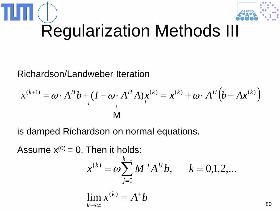
Regularization Methods III

Richardson/Landweber Iteration

( ))()()()1( )( kHkkHHk AxbAxxAAIbAx −⋅+=⋅−+⋅=+ ωωω

is damped Richardson on normal equations.

M

Assume x(0) = 0. Then it holds:

bAx k

k

+

∞→=)(lim

,...2,1,0,1

0

)( == ∑−

=

kbAMxk

j

Hjk ω

81

Proof

( )

( ) 01

0

1

0

1

0

∞→

++−

=

−

=

++−

=

+

→=

−−=

=−−=−

∑

∑∑

k

kk

j

HjH

k

j

HjHk

j

Hj

bMbAAAAII

AbAAAIbbAMb

ωω

ωωω

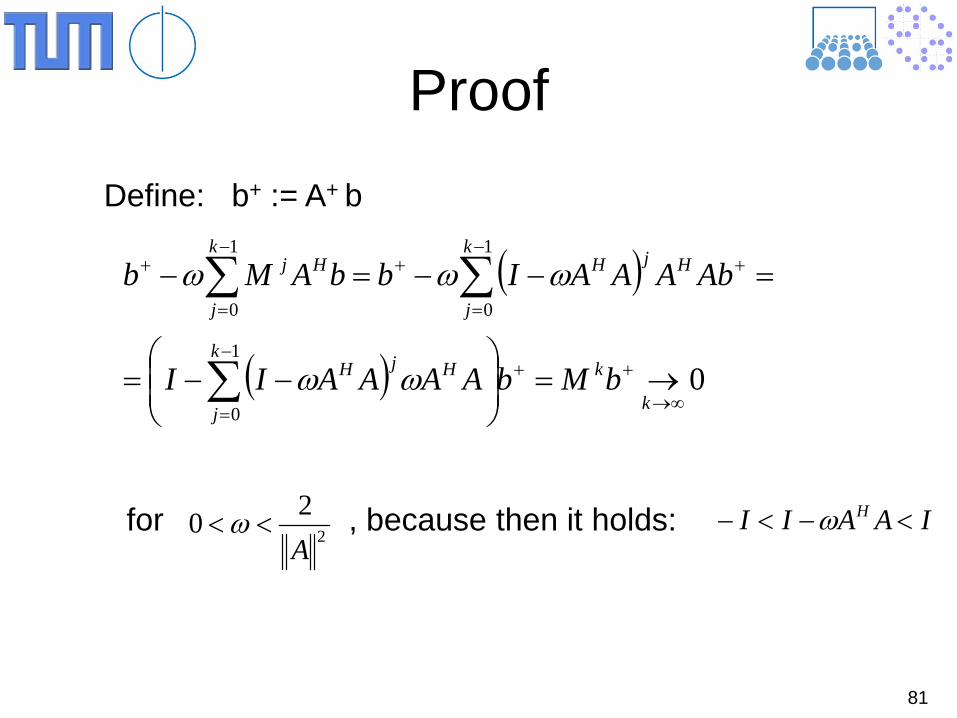
Define: b+ := A+ b

for , because then it holds: 2

20A

<<ω IAAII H <−<− ω

82

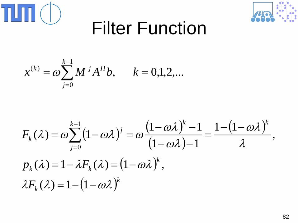
Filter Function

,...2,1,0,1

0

)( == ∑−

=

kbAMxk

j

Hjk ω

( ) ( )( )

( )

( )( )kk

kkk

kkk

j

jk

F

Fp

F

ωλλλ

ωλλλλ

λωλ

ωλωλωωλωλ

−−=

−=−=

−−=

−−−−

=−= ∑−

=

11)(

,1)(1)(

,1111111)(

1

0

83

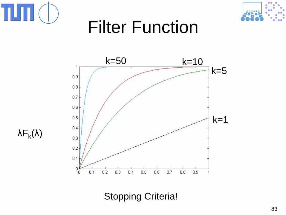
Filter Function

k=1

k=5 k=10 k=50

Stopping Criteria!

λFk(λ)

84

Projection Methods

Idea: If we know good approximate basis for signal subspace: Project linear system in this subspace and compute the solution of this projected linear system. Examples: Krylov subspace, Sine basis

Similarly: choose a set of smooth basis functions and consider the Galerkin projection of the original problem with these ansatz.

85

Regularization Methods IV Multigrid: Don‘t solve on high frequency components!

Conjugate Gradients:

In the first iteration steps: convergence relative to the large eigenvalues (signal subspace). Later iteration steps convergence relative to noise subspace! Stop!

86

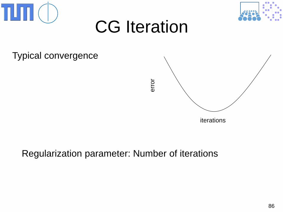
CG Iteration

Regularization parameter: Number of iterations

Typical convergence

erro

r

iterations

87

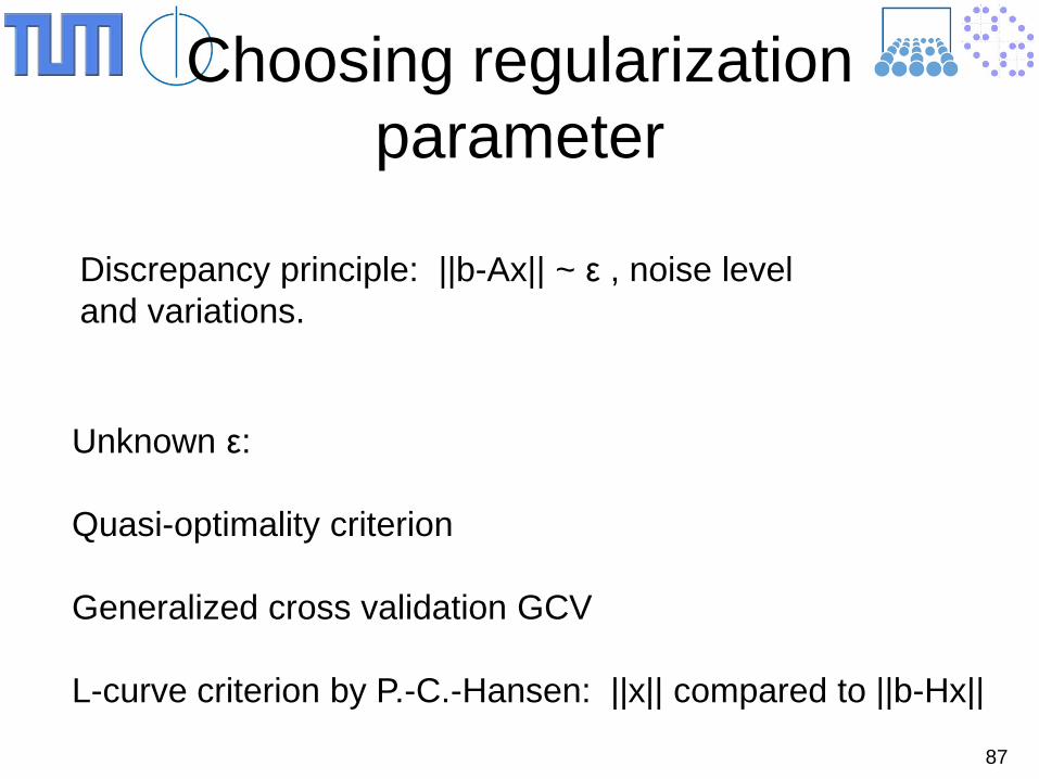
Choosing regularization parameter

Discrepancy principle: ||b-Ax|| ~ ε , noise level and variations.

Unknown ε: Quasi-optimality criterion Generalized cross validation GCV L-curve criterion by P.-C.-Hansen: ||x|| compared to ||b-Hx||

88

Discrepancy Principle

If we know the noise level ε , we know that is impossible to recover the original signal better than ε.

Consider monotonic sequence of regularization parameter ρk, that converges to 0 for k∞.

Compute the solution (Tikhonov, cg, …) starting with ρ1, ρ2,… until for the first time it holds ||Ax-b|| <≈ ε. Then stop and accept the related x as solution.

89

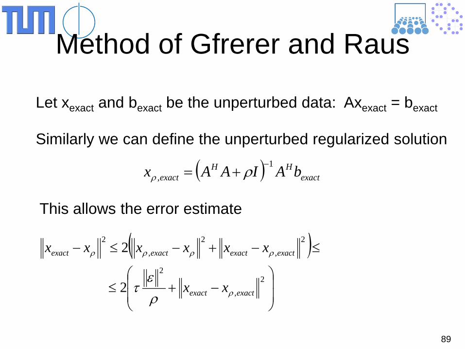
Method of Gfrerer and Raus

Let xexact and bexact be the unperturbed data: Axexact = bexact

Similarly we can define the unperturbed regularized solution

( ) exactHH

exact bAIAAx 1,

−+= ρρ

This allows the error estimate

( )

−+≤

≤−+−≤−

2,

2

2,

2,

2

2

2

exactexact

exactexactexactexact

xx

xxxxxx

ρ

ρρρρ

ρε

τ

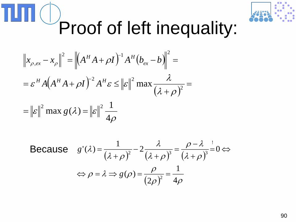
90

Proof of left inequality: ( ) ( )

( )( )

ρελε

ρλλεερε

ρρρ

41)(max

max

22

222

212,

==

=+

≤+=

=−+=−

−

−

g

AIAAA

bbAIAAxx

HHH

exHH

ex

Because ( ) ( ) ( )

( ) ρρρρλρ

ρλλρ

ρλλ

ρλλ

41

2)(

021)('

2

!

332

==⇒=⇔

⇔=+−

=+

−+

=

g

g

91

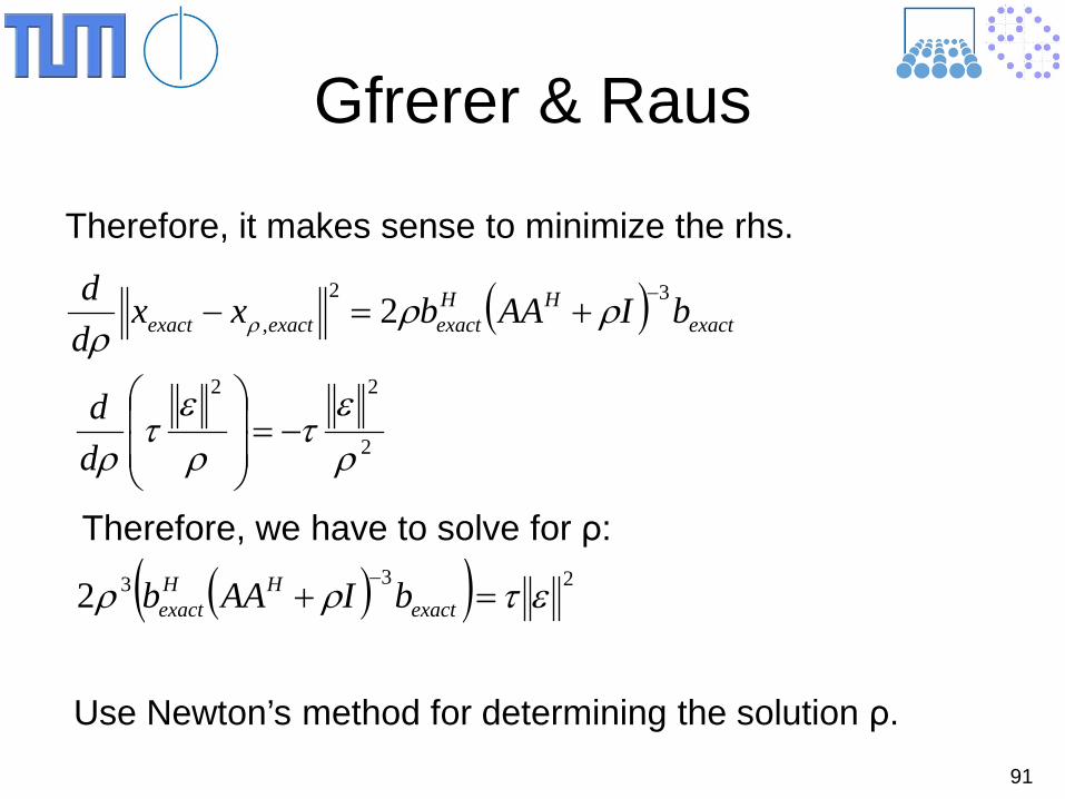
Gfrerer & Raus

Therefore, it makes sense to minimize the rhs.

( ) exactHH

exactexactexact bIAAbxxdd 32

, 2 −+=− ρρ

ρ ρ

2

22

ρε

τρε

τρ

−=

dd

Therefore, we have to solve for ρ:

( )( ) 2332 ετρρ =+−

exactHH

exact bIAAb

Use Newton’s method for determining the solution ρ.

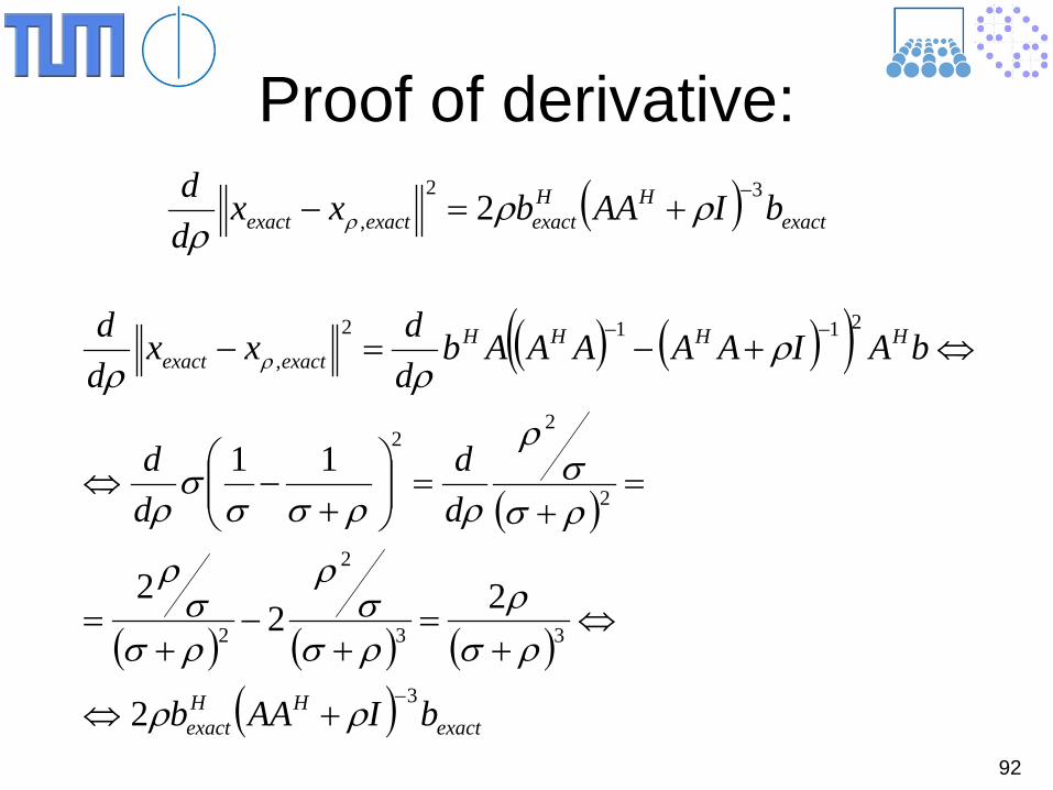
92

Proof of derivative: ( ) exact

HHexactexactexact bIAAbxx

dd 32

, 2 −+=− ρρ

ρ ρ

( ) ( )( )

( )

( ) ( ) ( )( ) exact

HHexact

HHHHexactexact

bIAAb

dd

dd

bAIAAAAAbddxx

dd

3

33

2

2

2

22

2112,

2

222

11

−

−−

+⇔

⇔+

=+

−+

=

=+

=

+

−⇔

⇔+−=−

ρρ

ρσρ

ρσσ

ρ

ρσσ

ρ

ρσσ

ρ

ρρσσσ

ρ

ρρρ ρ

93

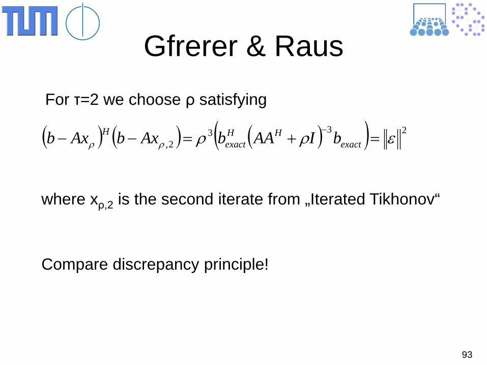
Gfrerer & Raus

( ) ( ) ( )( ) 2332, ερρρρ =+=−−

−

exactHH

exactH bIAAbAxbAxb

For τ=2 we choose ρ satisfying

where xρ,2 is the second iterate from „Iterated Tikhonov“

Compare discrepancy principle!

94

Proof: ( ) ( )

( )( ) ( ) ( )( )( )( )( ) ( ) ( )( )

( )

( )

( )( )( )exact

HHexact

HHHHHHH

HHHHH

HH

H

bIAAb

bAIAAAIAAAIAIAAAIb

bAIAAbAIAAAbbAIAAAb

AxbAxb

333

3

2

222

2

211

111

2,

2

11

−

−−−

−−−

+⇔+

=

=+

−−−++⋅

+=

=

+−

+−

+

−⇔

⇔+−+−+−=

=+++−+−=

=−−

ρρρσ

ρρσ

ρσρσσρρσσρσ

ρ

ρσσρ

ρσσ

ρσσ

ρρρρ

ρρρρ

ρρ

95

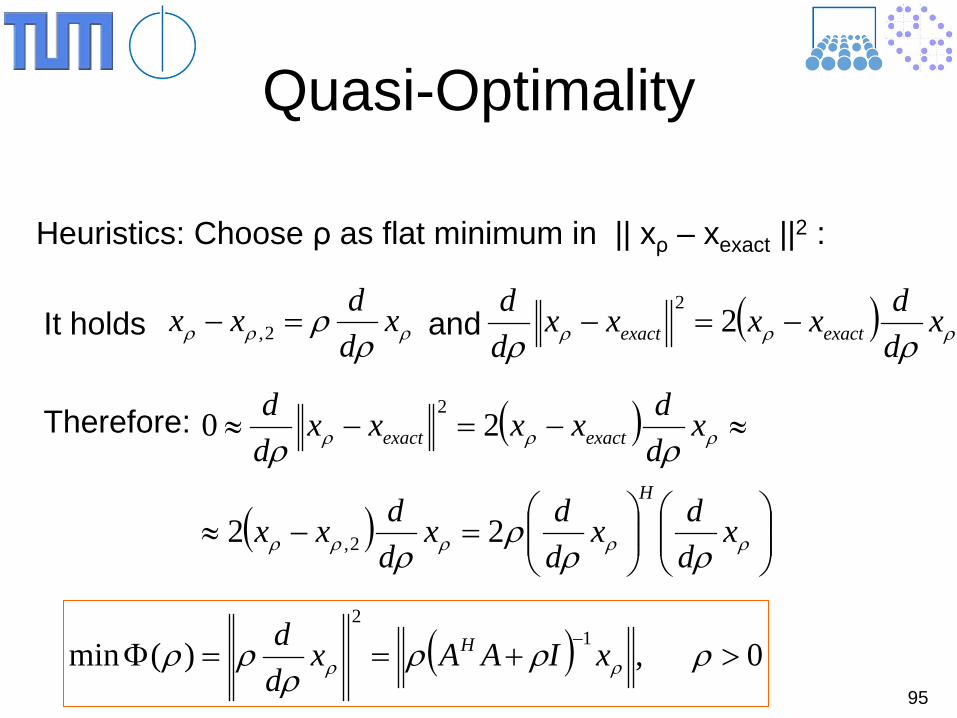
Quasi-Optimality

Heuristics: Choose ρ as flat minimum in || xρ – xexact ||2 :

( ) 0,)(min 12

>+==Φ−

ρρρρ

ρρ ρρ xIAAxdd H

It holds and ρρρ ρρ x

ddxx =− 2, ( ) ρρρ ρρ

xddxxxx

dd

exactexact −=− 22

Therefore: ( )

( )

=−≈

≈−=−≈

ρρρρρ

ρρρ

ρρρ

ρ

ρρ

xddx

ddx

ddxx

xddxxxx

dd

H

exactexact

22

20

2,

2

96

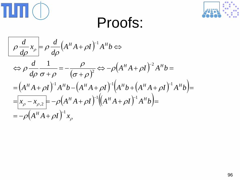
Proofs: ( )

( )( )

( ) ( ) ( )( )( ) ( )( )

( ) ρ

ρρ

ρ

ρρ

ρρρ

ρρρ

ρρρσ

ρρσρ

ρ

ρρ

ρρ

ρ

xIAA

bAIAAIAAxx

bAIAAbAIAAbAIAA

bAIAAdd

bAIAAddx

dd

H

HHH

HHHHHH

HH

HH

1

112,

111

2

2

1

1

−

−−

−−−

−

−

+−=

=++−=−=

=+++−+=

=+−⇔+

−=+

⇔

⇔+=

97

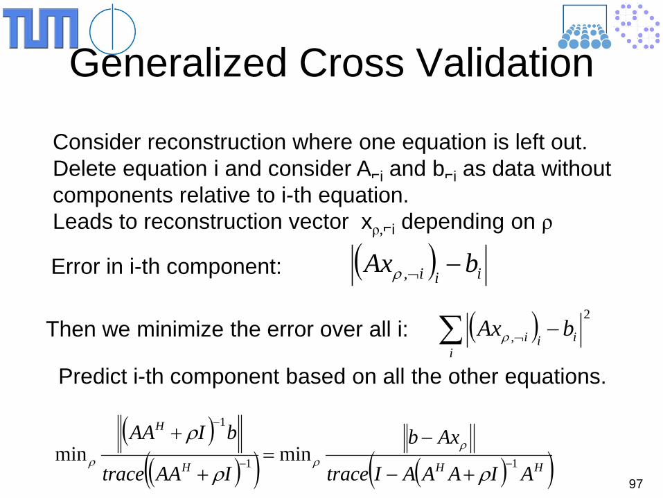
Generalized Cross Validation

Consider reconstruction where one equation is left out. Delete equation i and consider Ai and bi as data without components relative to i-th equation. Leads to reconstruction vector xρ,i depending on ρ

Then we minimize the error over all i: ( )∑ −¬i

iii bAx2

,ρ

( ) iii bAx −¬,ρError in i-th component:

( )( )( ) ( )( )HHH

H

AIAAAItrace

Axb

IAAtrace

bIAA11

1

minmin −−

−

+−

−=

+

+

ρρ

ρρ

ρρ

Predict i-th component based on all the other equations.

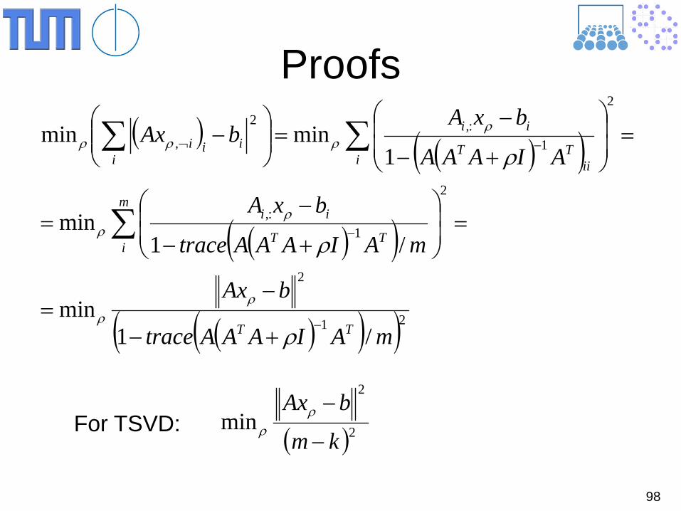
98

Proofs ( ) ( )( )

( )( )

( )( )( )21

2

2

1:,

2

1:,2

,

/1min

/1min

1minmin

mAIAAAtrace

bAx

mAIAAAtrace

bxA

AIAAA

bxAbAx

TT

m

iTT

ii

i iiTT

ii

iiii

−

−

−¬

+−

−=

=

+−

−=

=

+−

−=

−

∑

∑∑

ρ

ρ

ρ

ρρ

ρρ

ρρρρ

For TSVD: ( )22

minkm

bAx

−

−ρρ

99

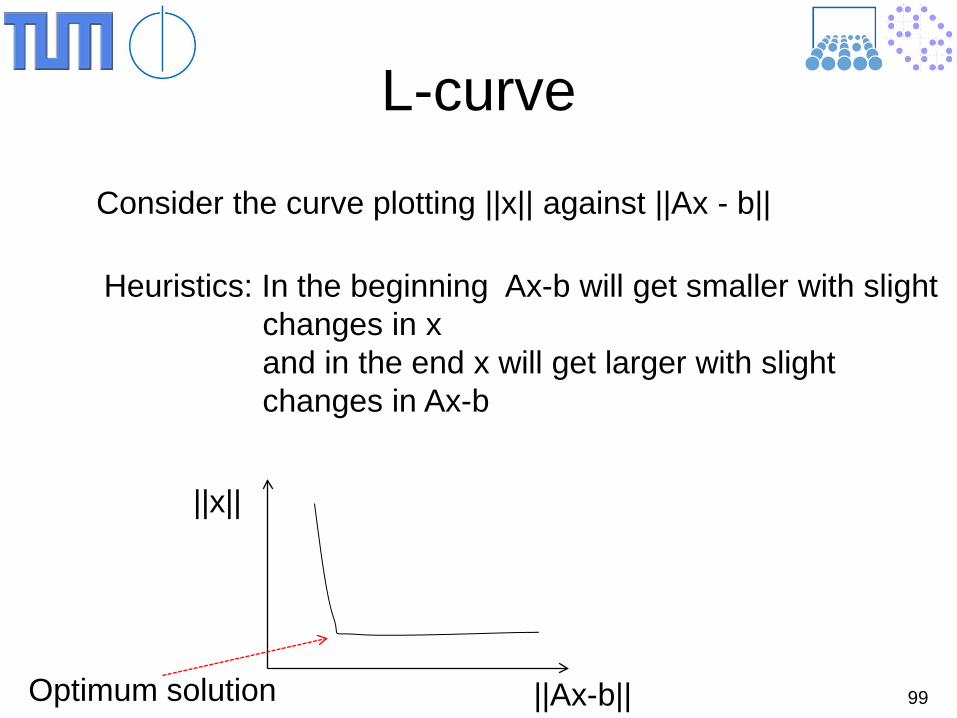
L-curve

Consider the curve plotting ||x|| against ||Ax - b||

Heuristics: In the beginning Ax-b will get smaller with slight changes in x and in the end x will get larger with slight changes in Ax-b

||Ax-b||

||x||

Optimum solution

100

L-curve practical To enforce the L-shape of the curve we use a log-log scaling.

Right side: horizontal part is related to dominating regularization, not all information extracted Left side: vertical part is dominated by perturbation error, noise destroys the signal Optimum in the corner balancing both.

To estimate corner: Approximate curve by Splines. Determine point with maximum curvature

101

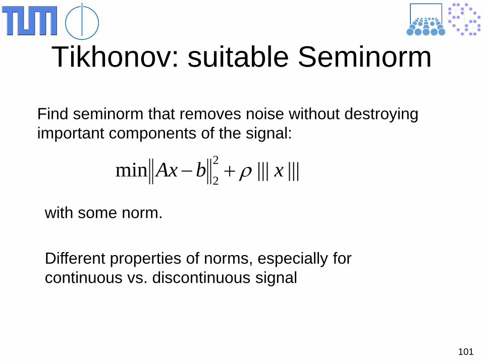
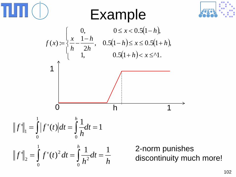
Tikhonov: suitable Seminorm

Find seminorm that removes noise without destroying important components of the signal:

||||||min 2

2xbAx ρ+−

with some norm.

Different properties of norms, especially for continuous vs. discontinuous signal

102

Example ( )

( ) ( )( )

≤<+

+≤≤−−

−

−<≤

=

.1^15.0,1

,15.015.0,2

1,15.00,0

:)(

xh

hxhhh

hx

hx

xf

h

1

1 0

11)(''0

1

01

=== ∫∫ dth

dttffh

hdt

hdttff

h 11)(''0

2

1

0

22

=== ∫∫2-norm punishes discontinuity much more!

103

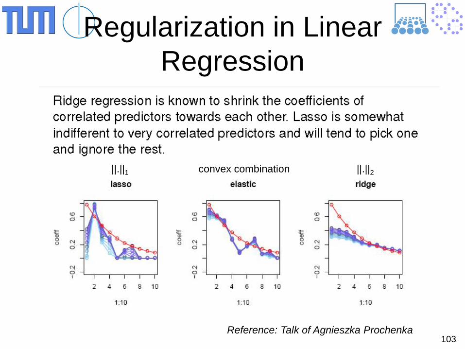
Regularization in Linear Regression

Reference: Talk of Agnieszka Prochenka

||.||1 convex combination ||.||2

104

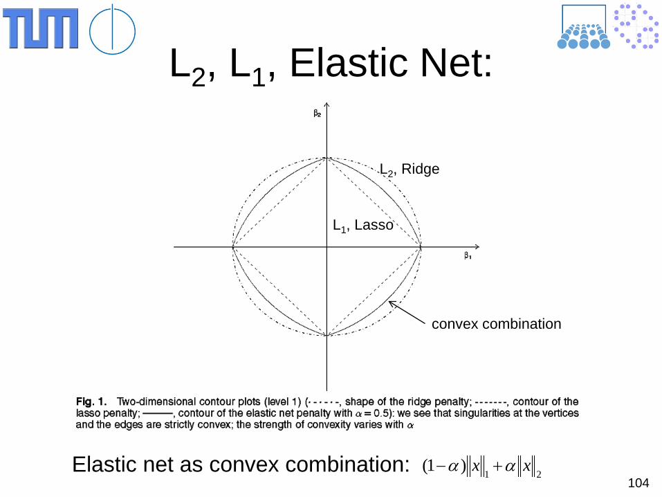
L2, L1, Elastic Net:

L2, Ridge

convex combination

L1, Lasso

Elastic net as convex combination: 21)1( xx αα +−

105

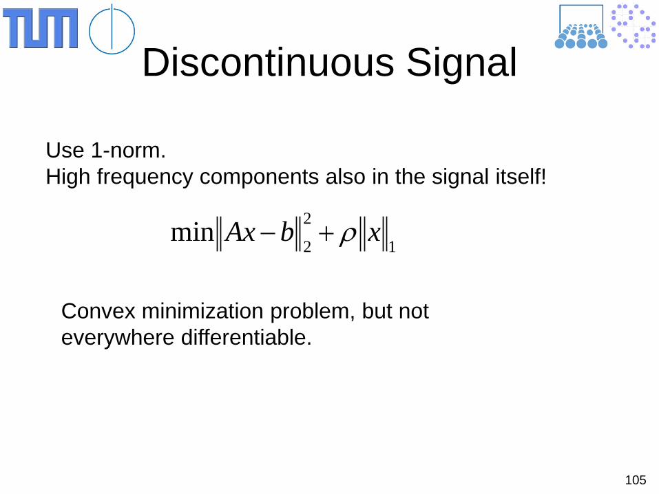
Discontinuous Signal

Use 1-norm. High frequency components also in the signal itself!

1

2

2min xbAx ρ+−

Convex minimization problem, but not everywhere differentiable.

106

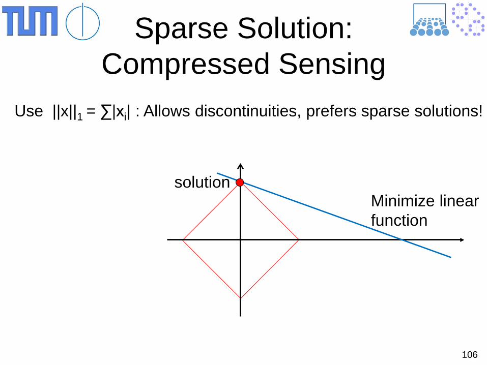
Sparse Solution: Compressed Sensing

Use ||x||1 = ∑|xi| : Allows discontinuities, prefers sparse solutions!

Minimize linear function

solution

107

Continuous Signal

The seminorm ||Lx|| should vanish near the signal Subspace but penalize the noise subspace.

Therefore, L should model the derivative!

108

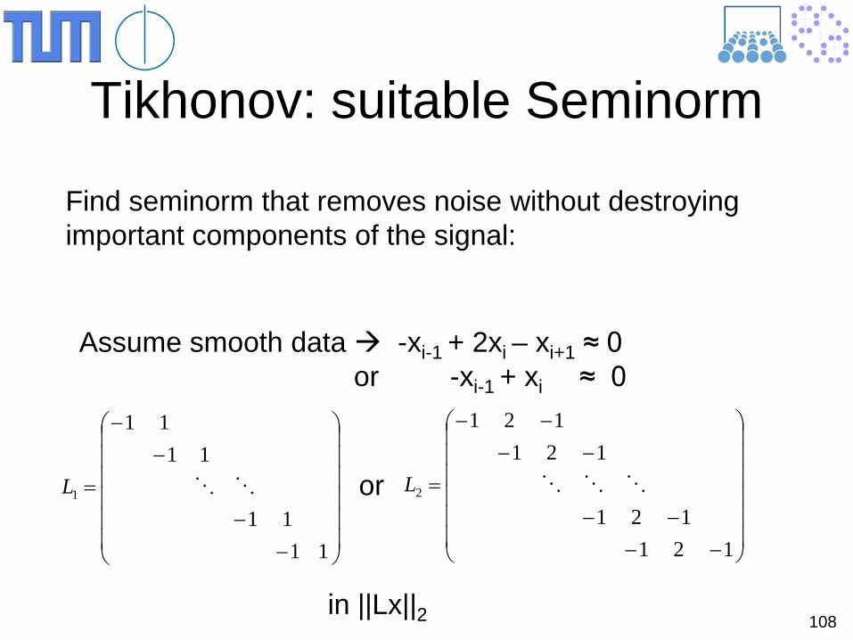
Tikhonov: suitable Seminorm

Find seminorm that removes noise without destroying important components of the signal:

Assume smooth data -xi-1 + 2xi – xi+1 ≈ 0 or -xi-1 + xi ≈ 0

−−−−

−−−−

=

121121

121121

2 L

−−

−−

=

1111

1111

1 L or

in ||Lx||2

109

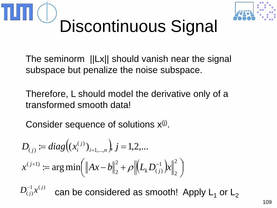
Discontinuous Signal

The seminorm ||Lx|| should vanish near the signal subspace but penalize the noise subspace.

Therefore, L should model the derivative only of a transformed smooth data!

( )( )

+−=

==

−+

=

2

2

1)(

2

2)1(

,...,1)(

)(

minarg:

,...2,1,)(:

xDLbAxx

jxdiagD

jkj

nij

ij

ρ

Consider sequence of solutions x(j).

)(1)(

jj xD−

can be considered as smooth! Apply L1 or L2

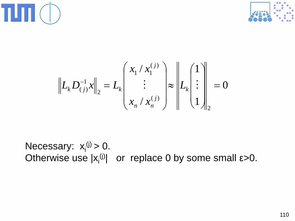
110

01

1

/

/

2)(

)(11

2

1)( =

≈

=− kj

nn

j

kjk Lxx

xxLxDL

Necessary: xi(j) > 0.

Otherwise use |xi(j)| or replace 0 by some small ε>0.

111

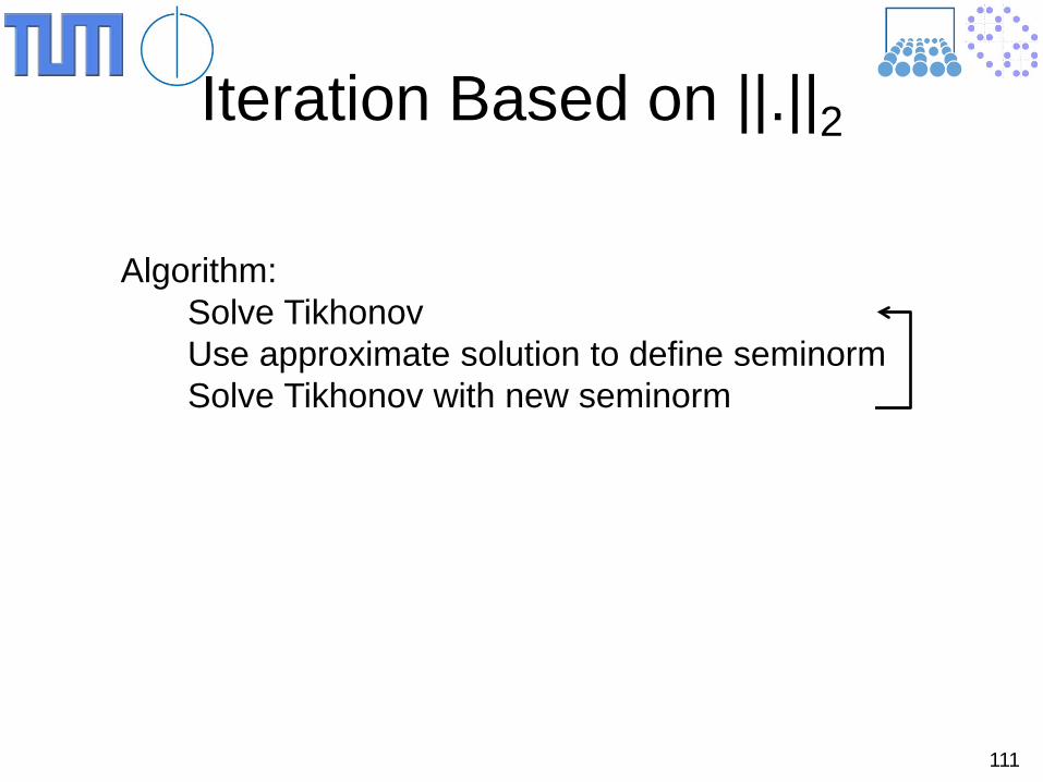
Iteration Based on ||.||2

Algorithm: Solve Tikhonov Use approximate solution to define seminorm Solve Tikhonov with new seminorm

112

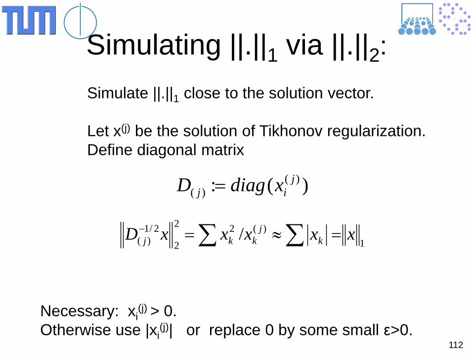
Simulating ||.||1 via ||.||2:

Simulate ||.||1 close to the solution vector. Let x(j) be the solution of Tikhonov regularization. Define diagonal matrix

)(: )()(

jij xdiagD =

1)(22

2

2/1)( / xxxxxD k

jkkj ∑∑ =≈=−

Necessary: xi(j) > 0.

Otherwise use |xi(j)| or replace 0 by some small ε>0.

113

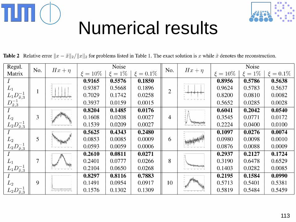
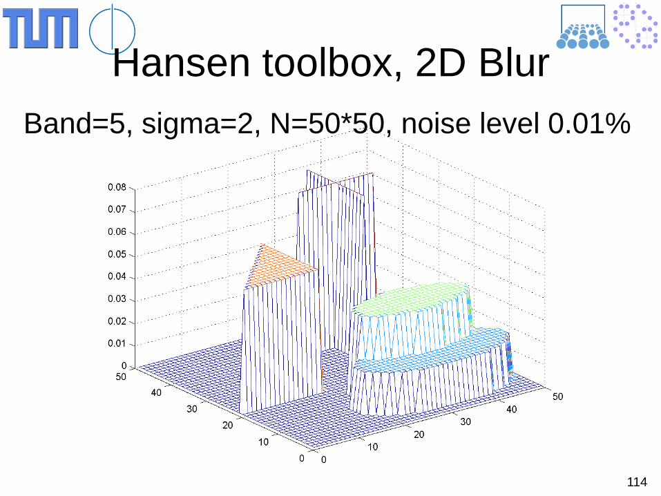
Numerical results

114

Hansen toolbox, 2D Blur Band=5, sigma=2, N=50*50, noise level 0.01%

115

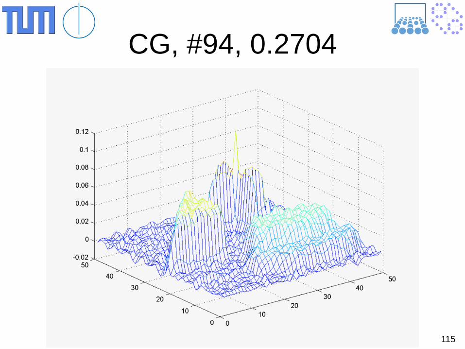
CG, #94, 0.2704

116

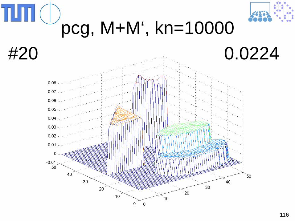
pcg, M+M‘, kn=10000 #20 0.0224

117

Idea for definition of L for nonsmooth signal: Compute approximate solution x(1). Define seminorm L(1), such that L(1)x(1)=0

Compute approximate solution x(2).

repeat

Advantage: on the signal subspace the seminorm has no influence

Similar Approach

118

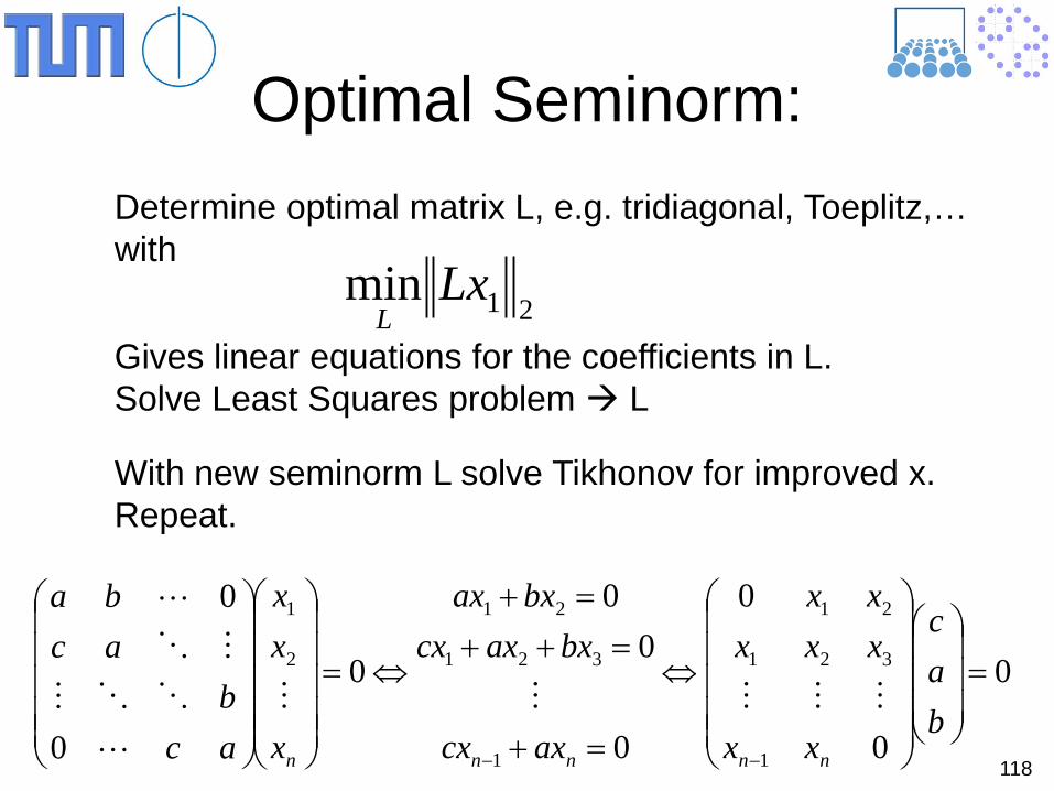
Optimal Seminorm: Determine optimal matrix L, e.g. tridiagonal, Toeplitz,… with

21min LxL

Gives linear equations for the coefficients in L. Solve Least Squares problem L

With new seminorm L solve Tikhonov for improved x. Repeat.

0

0

0

0

00

0

0

0

1

321

21

1

321

21

2

1

=

⇔

=+

=++=+

⇔=

−−

bac

xx

xxxxx

axcx

bxaxcxbxax

x

xx

acb

acba

nnnnn

119

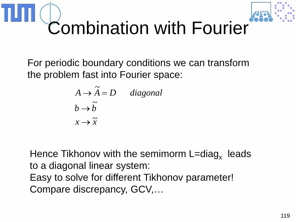
Combination with Fourier

For periodic boundary conditions we can transform the problem fast into Fourier space:

xxbb

diagonalDAA

~

~

~

→→

=→

Hence Tikhonov with the semimorm L=diagx leads to a diagonal linear system: Easy to solve for different Tikhonov parameter! Compare discrepancy, GCV,…

120

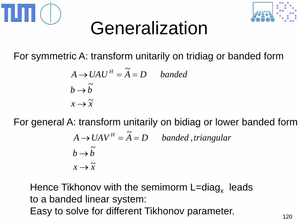
Generalization For symmetric A: transform unitarily on tridiag or banded form

xxbb

bandedDAUAUA H

~

~

~

→→

==→

Hence Tikhonov with the semimorm L=diagx leads to a banded linear system: Easy to solve for different Tikhonov parameter.

For general A: transform unitarily on bidiag or lower banded form

xxbb

triangularbandedDAUAVA H

~

~,~

→→

==→

121

Preconditioner vs Seminorm

( )( )

⇔=+−⇔

⇔=+⇔

⇔=+⇔

⇔+−

−

−−−

LxyybyAL

bALLxIALALbAxLLAA

LxbAx

TTTT

TTT

,min

)(

min

2

222

2

1

21

2

2

222

2

ρ

ρ

ρ

ρ

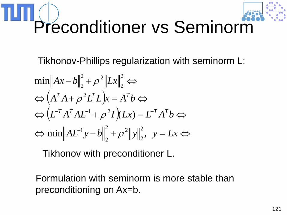
Tikhonov-Phillips regularization with seminorm L:

Tikhonov with preconditioner L.

Formulation with seminorm is more stable than preconditioning on Ax=b.

122

(2) Preconditioning relative to a subspace

Explicit preconditioners relative to A: - Jacobi - Gauss-Seidl - ILU - MILU

Implicit preconditioners relative to A-1: - Polynomial preconditioner - SPAI,FSAI - MSPAI

Probing, method of action Filtering decomposition

123

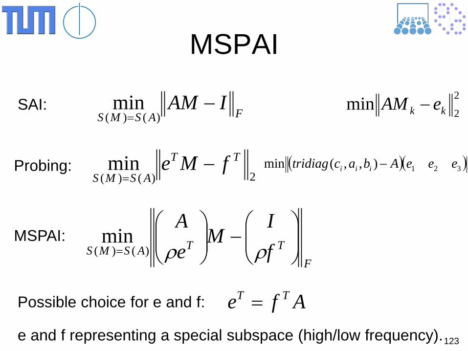
MSPAI

FASMSIAM −

= )()(minSAI:

2)()(min TT

ASMSfMe −

=Probing:

MSPAI:

FTTASMS f

IM

eA

−

= ρρ)()(

min

Possible choice for e and f: Afe TT =

e and f representing a special subspace (high/low frequency).

2

2min kk eAM −

( )( )321),,(min eeeAbactridiag iii −

124

MSPAI Probing

Advantage compared to classical probing / method of action: We don’t have to care about the unique solvability of the probing conditions.

Not necessarily 3 probing vectors for tridiagonal preconditioner!

Freedom to choose any vector and any matrix pattern!

125

Probing vectors

Vector f-=(1,-1,1,-1,..…) representing the high frequency part related to large eigenvalues/noise.

Vector f+=(1,1,1,1,..…) representing the low frequency part related to small eigenvalues/signal.

We are looking for a preconditioner esp. for large eigenvalues, resp. smooth probing vectors, that should be zero or I for noisy probing vectors.

126

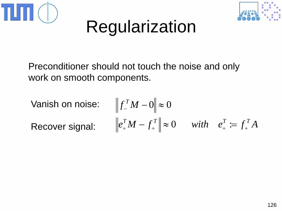
Regularization

Preconditioner should not touch the noise and only work on smooth components.

AfewithfMe

MfTTTT

T

++++

−

=≈−

≈−

:0

00Vanish on noise: Recover signal:

127

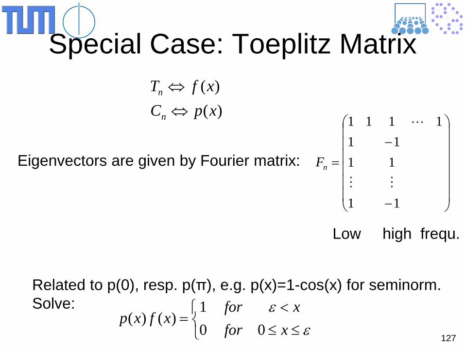
Special Case: Toeplitz Matrix

)()(

xpCxfT

n

n

⇔⇔

Eigenvectors are given by Fourier matrix:

−

−=

11

1111

1111

nF

Low high frequ.

Related to p(0), resp. p(π), e.g. p(x)=1-cos(x) for seminorm. Solve:

≤≤<

=ε

εxfor

xforxfxp

001

)()(

128

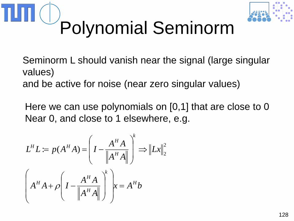
Polynomial Seminorm Seminorm L should vanish near the signal (large singular values) and be active for noise (near zero singular values)

Here we can use polynomials on [0,1] that are close to 0 Near 0, and close to 1 elsewhere, e.g.

bAxAAAAIAA

LxAAAAIAApLL

H

k

H

HH

k

H

HHH

=

−+

⇒

−==

ρ

2

2)(:

129

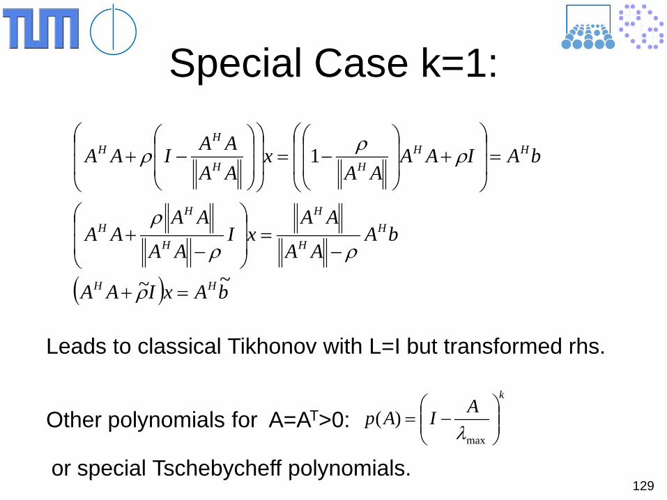
Special Case k=1:

( ) bAxIAA

bAAA

AAxI

AA

AAAA

bAIAAAA

xAAAAIAA

HH

HH

H

H

HH

HHHH

HH

~~

1

=+

−=

−+

=

+

−=

−+

ρ

ρρ

ρ

ρρρ

Leads to classical Tikhonov with L=I but transformed rhs.

Other polynomials for A=AT>0: k

AIAp

−=

max

)(λ

or special Tschebycheff polynomials.

ill-posed inverse problems and regularization methods · ill-posed inverse problems and...

Documents