carbon dioxide thickening agents for …carbon dioxide thickening agents for reduced co 2 mobility...
TRANSCRIPT
CARBON DIOXIDE THICKENING AGENTS FOR REDUCED CO2 MOBILITY
by
Jianhang Xu
B.S. in Ch.E., East China University of Science and Technology, 1992
M.S. in Ch.E., East China University of Science and Technology, 1995
Submitted to the Graduate Faculty of
the School of Engineering in partial fulfillment
of the requirements for the degree of
Doctor of Philosophy
University of Pittsburgh
2003
ii
UNIVERSITY OF PITTSBURGH
SCHOOL OF ENGINEERING
This dissertation was presented
by
Jianhang Xu
It was defended on
February, 20, 2003
and approved by
Eric Beckman, Professor, Department of Chemical Engineering
Badie Morsi, Professor, Department of Chemical Engineering
Patrick Smolinski, Professor, Department of Mechanical Engineering
Dissertation Director: Robert Enick, Professor, Department of Chemical Engineering

iii
ABSTRACT
CARBON DIOXIDE THICKENING AGENTS FOR REDUCED CO2 MOBILITY
Jianhang Xu, PhD
University of Pittsburgh, 2003
The objective of this work is to design, synthesize, and evaluate direct carbon dioxide
thickeners. The thickener must dissolve in CO2 without the introduction of a cosolvent. The
thickener, in dilute solution of less than one weight percent, should be capable of at least
doubling the viscosity of dense CO2 at temperature and pressure conditions characteristic of
CO2 EOR floods.
A bulk-polymerized, random copolymer of fluoroacrylate (71mol%) and styrene
(29mol%), Mn=540,000, has been identified as an efficient CO2 thickener using falling
cylinder viscometry and flow-through-porous-media viscometry. For example, a 0.5wt%
solute of the random copolymer in CO2 tripled the viscosity of liquid CO2 flowing through a
100md sandstone core at superficial velocities of 1~10ft/day.
Non-fluorous polymers are also investigated in an attempt to identify a less
expensive, more environmentally benign thickener. Our first step is to identify a highly CO2-
philic, hydrocarbon-based polymer. Among all commodity polymers, poly vinyl acetate,
PVAc, is identified as the most CO2 soluble, non-fluorous, hydrocarbon-based commercial
available polymer. Nonetheless, PVAc does not exhibit sufficient solubility in CO2 at
reservoir conditions to form the basis of a class of CO2 thickeners.

iv
ACKNOWLEDGMENTS
I want to express my gratitude to my research advisor Dr. Enick for his guidance
and encouragement throughout my studies at the University of Pittsburgh. He has been
more than an advisor, a friend and a mentor whom I have learned so much from. I would
also like to thank Dr. Beckman for his resourceful suggestion and endless
encouragement. I would also thank my committee members Dr. Morsi, and Dr. Smolinski
for their constructive criticism and suggestion.
I would like to thank Chemical Engineering Department at the University of
Pittsburgh for the fellowship for my PhD study here. I wish to express my appreciation to
U.S. Department of Energy for the financial support for this project.
I am very grateful to the faculty, staff and friends in the chemical engineering
department. Especially, I want to thank Ron Bartlett and Bob Maniet for their help in
setting up the experiment apparatus.
Finally, I would like to dedicate this work to my parents, who have been always
encouraging me in my education.
v
TABLE OF CONTENTS
1.0 INTRODUCTION .……………………………………………………………………...1
1.1. Enhanced Oil Recovery (EOR) ……………………………………………………..1
1.2 CO2 for Formation Fracturing ……………………………………………………….7
2.0 LITERATURE REVIEW AND BACKGROUND ..…………………………………….8
2.1 WAG …………………………………………………………………………………8
2.2 Previous attempts to increase the viscosity of CO2…………………………………..9
2.2.1 Entrainers (cosolvents) ……………………………………………………..9
2.2.2 In-situ polymerization of CO2 soluble monomers …………………………9
2.2.3 Small, Associating Compounds …………………………………………..10
2.2.4 Dissolution of conventional polymers into CO2 ………………………….12
2.3 Solubility of Polymers and Copolymers in Supercritical CO2 ……………………..15
3.0 APPROACH ..…………………………………………………………………………..19
3.1 Fluorous CO2 thickener ……………………………………………………………..19
3.2 Non-fluorous CO2 thickeners ……………………………………………………….20
3.3 Non-fluorous homopolymer ………………………………………………………...22
4.0 THICKENING CANDIDATES .………………………………………………………..24
4.1 Fluoroacrylate-styrene copolymer …………………………………………………..24
4.1.1 Material and methods ……………………………………………………...24
4.1.2 3M Fluoroacrylate styrene copolymer …………………………………….25

vi
4.1.3 Random Styrene-FA-x Copolymer ………………………………………..26
4.2 Butadiene-Acetate copolymers ……………………………………………………...26
4.3 Other non-fluorous polymers ………………………………………………………..29
4.3.1 Materials and Methods …………………………………………………….29
4.3.2 Characterization …………………………………………………………...31
5.0 SOLUBILITY APPARATUS….………………………………………………………..32
6.0 FALLING CYLINDER VISCOMETER ..……………………………………………...35
6.1 Friction factor ……………………………………………………………………….38
6.2 Reynolds number ……………………………………………………………………40
6.3 Theoretical and experimental calibration constants …………………………………40
7.0 FLOW-THROUGH-POROUS-MEDIA VISCOMETER .……………………………...44
7.1 Experimental apparatus ……………………………………………………………...44
7.2 Berea sandstone core ………………………………………………………………...48
7.3 Core holder …………………………………………………………………………..48
7.4 Pressure transducer ………………………………………………………………….49
8.0 FLUORINATED POLYMER RESULTS .……………………………………………..51
8.1 Solubility results …………………………………………………………………….51
8.1.1 Polyfluoroacrylate and polyfluoroacrylate-styrene copolymer …………...51
8.1.2 Styrene-FA-x copolymer solubility ……………………………………….52
8.1.3 Temperature effect on the fluoroacrylate-styrene copolymer
solubility ………………………………………………………………...55
8.2 Falling cylinder viscometer results ………………………………………………….57
8.2.1 Aldrich fluoroacrylate-styrene copolymer ………………………………...57
vii
8.2.2 3M fluoroacrylate-styrene copolymer ……………………………………59
8.2.3 Temperature effect on the fluoroacrylate-styrene copolymer
thickening ability ………………………………………………………60
8.2.4 Non-Newtonian fluid …………………………………………………….61
8.3 Flow-through-porous-media viscometer results …………………………………...65
9.0 NON-FLUOROUS POLYMER RESULTS ..………………………………………….72
9.1 Polypropylene oxide, PPO …………………………………………………………73
9.2 Polybutadiene ………………………………………………………………………74
9.3 Polyethoxyethyl acrylate ……………………………………………………………75
9.4 Polybutoxyethyl acrylate ……………………………………………………………76
9.5 Polyvinyl ester ( VeoVa 10 monomer ) ……………………………………………..76
9.6 Poly vinyl acetate, PVAc ……………………………………………………………77
9.7 Polymethyl acrylate, PMA …………………………………………………………..83
9.8 Poly vinyl formate, PVF …………………………………………………………….87
9.9 Methyl isobutyrate (MIB) and isopropyl acetate (IPA) …………………………….88
9.10 Poly dimethyl siloxane …………….……………………………………..………..90
10.0 CONCLUSION AND FUTURE WORK..……………………………………………..92
APPENDIX A. NEWTONIAN FLUID MODEL DEVELOPMENT..………….….………95
APPENDIX B. NON-NEWTONIAN FLUID MODEL DEVELOPMENT .……………..107
APPENDIX C. C++ PROGRAM FOR POWER-LAW MODEL…………………………113
APPENDIX D. MATLAB PROGRAM FOR FALLING CYLINDER VISCOMETER
CALIBRATION …………………………………………………………..117
BIBLIOGRAPHY …………………………………………………………………………121

viii
LIST OF TABLES Table No Page 6.1 Falling cylinder viscometer dimensions ……………………………………………36
8.1 Molecular weight of fluoropolymers ………………………………………………52
8.2 Temperature effect on the solution relative viscosity ……………………………...60
8.3 Experimental falling cylinder terminal velocity ……………………………………61
8.4 Power law model constants (m, s=1/n) …………………………………………….62
8.5 Berea core flooding results …………………………………………………………68
9.1 Molecular weight of PMA, PVAc and PPO ………………………………………..91

ix
LIST OF FIGURES Figure No Page 1.1 Minimum miscibility pressure (MMP) ……………………………………………4
1.2 Viscosity of carbon dioxide ………………………………………………………5
1.3 Viscous miscible fingering ……………………………………………………….6
4.1 Synthesis of the fluoroacrylate-styrene random copolymer ……………………..25
4.2 Synthesis of partly dihydroxylized polybutadiene ………………………………27
4.3 Synthesis of partly functionalized dihydroxylized polybutadiene ……………….28
4.4 Synthesis of partly epoxylized polybutadiene ……………………………………28
4.5 Synthesis of hydroxylized polybutadiene ………………………………………..28
4.6 Synthesis of partly acetated polybutadiene ………………………………………29
5.1 High pressure, variable volume, windowed cell (D.B. Robinson Cell) ………….34
6.1 Viscosity measurement …………………………………………………………..37
6.2 Friction factor vs. Reynolds number ……………………………………………..39
6.3 Experiment calibration constant vs. theoretical constant ………………………...43
7.1 Permeability apparatus …………………………………………………………...47
7.2 Berea sandstone core ……………………………………………………………..47
7.3 Core holder ……………………………………………………………………….50
8.1 Fluoroacrylate-styrene copolymer cloud point vs. concentration (T=297K) …….53
8.2 Solubility of polyFA and fluoroacrlate-styrene copolymer in carbon dioxide

x
at 298K……………………………………………………………………………54
8.3 Effect of temperature on the solubility of the fluoroacrylate-styrene copolymer
in carbon dioxide …………………………………………………………………56
8.4 Relative viscosity vs. shear rate ………………………………………………….58
8.5 Relative viscosity vs. shear rate (3M copolymer) ………………………………..59
8.6 Power law constant s, n(=1/s) (T=297K, P=34MPa) …………………………….63
8.7 Power law constant m (T=297K, P=34MPa) …………………………………….64
8.8 Relative viscosity vs. shear rate (power law) …………………………………….66
8.9 Relative viscosity increase vs. concentration at 298K, 20MPa,
flowing through ~100md Berea sandstone ………………………………………69
8.10 CO2 flooding at 3500psi and 1ft/day …………………………………………….70
8.11 CO2 flooding at 3500psi and 10ft/day …………………………………………...71
9.1 Propylene oxide monomer and homopolymer structure …………………………73
9.2 Cloud point curve for ~5wt% poly(propylene oxide)
(PPO, Mw=3500)-CO2 mixture …………………………………………………74
9.3 Butadiene monomer and homopolymer, and acetate end-capped polyBD ……...75
9.4 2-ethoxyethyl acrylate monomer and homopolymer ……………………………75
9.5 Butozyethyl acrylate monomer and homopolymer ……………………………...76
9.6 VeoVa 10 monomer and homopolymer …………………………………………77
9.7 Vinyl acetate monomer and homopolymer structure ……………………………77
9.8 Effect of polymer molecular weight on the cloud point curves
for ~5wt% poly(vinyl acetate) (PVAc)-CO2 mixtures ………………………….81
9.9 Phase behavior of PVA, PPO, and PMA at 298K ………………………………82

xi
9.10 Methyl acrylate monomer and homopolymer …………………………………..83
9.11 Pressure composition isotherms for the system CO2-poly(methyl acrylate) (PMA)
(Mw=2850) at 298, 313, 323K ……………………………………………………85
9.12 Cloud point pressure at ~5wt% polymer concentration and 298K for binary mixture
of CO2 with poly(methyl acrylate) (PMA), poly(lactide) (PLA), poly(vinyl acetate)
(PVAc), poly(dimethyl siloxane) (PDMS), and poly(fluoroalkyl acrylate) (PFA)
as a function of number of repeat units based on Mw ……………………………86
9.13 Vinyl formate monomer and hompolymer ………………………………………...87
9.14 Methyl isobutyrate and isopropyl acetate ………………………………………….88
9.15 Phase behavior of methyl isobutyrate and isopropyl acetate in CO2 (T=323K), critical
point in the 3-5wt% range …………………………………………………………89
9.16 Poly(dimethyl siloxane) structure …………………………………………………90

1
1.0 INTRODUCTION
Oil is an important energy source. All over the world, the demand for petroleum products
has continued to rise. In Europe and North America, most of the easily exploitable petroleum
reservoirs have already been found and overall production is in decline. Therefore, it is becoming
more important to get more oil with enhanced oil recovery from existing fields. Several
mechanisms are employed in the recovery of crude oil. Primary production, producing oil under
its own pressure and/or by the expansion of the dissolved gas, accounts the recovery of 5-20% of
the oil. Secondary production, the injection of water to displace the oil, can recover nearly 50%
of the oil. There are several tertiary methods employed after water flooding that may be
considered to recover the remaining oil.
1.1 Enhanced Oil Recovery (EOR)
Enhanced or improved oil recovery processes employ fluids other than water to recover
oil, and are referred to as tertiary processes if they are employed after water flooding. EOR
methods include hydrocarbon miscible flooding, CO2 flooding, polymer flooding, steam
flooding, immiscible gas injection. They inject different fluids to displace additiona l oil from
reservoir, via several mechanisms including: solvent extraction to achieve (or approach)
miscibility, interfacial-tension (IFT) reduction, improved sweep efficiency, pressure
maintenance, oil swelling, and viscosity reduction.[1]

2
Among these EOR methods, gas or vapor flooding dominates the EOR production. More
than 75% of the EOR projects in North America involve injection of steam, CO2, or light
hydrocarbon solvents. Due to the expense of hydrocarbon-based solvents, such as LPG, few
hydrocarbon miscible floods are currently conducted. Steam flooding is typically applied to
heavy, viscous crude oils that require substantial viscosity reduction. Carbon dioxide is typically
applied to post-water flooded oil fields that retain significant amount of light oils.[2] CO2
flooding has many advantages that have made it a widely employed EOR technique in the
southern US. CO2 is environmentally benign, available in large amount from natural reservoirs,
inexpensive, nonflammable, and non-toxic except as an asphyxiant. A large number of field
applications have been initiated in the past decade, especially in Texas and New Mexico.
Currently, roughly 1.2 billion SCF of CO2 are injected into domestic reservoirs each day.
The main disadvantage of CO2 flooding is its low viscosity, which can contribute to low
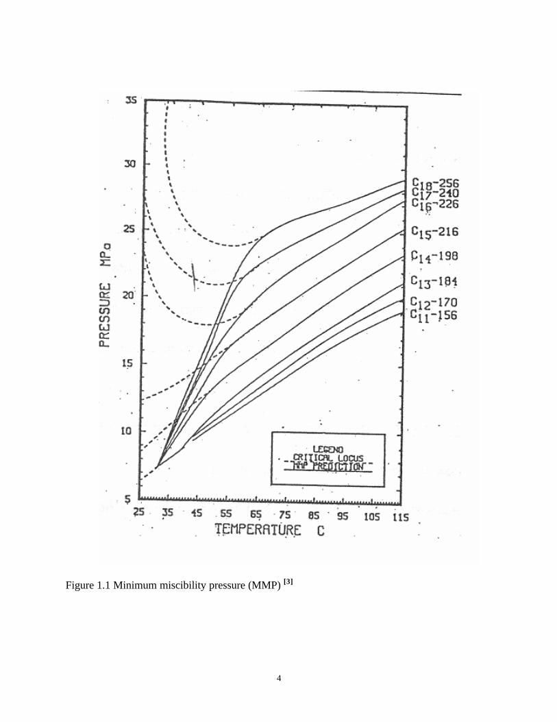
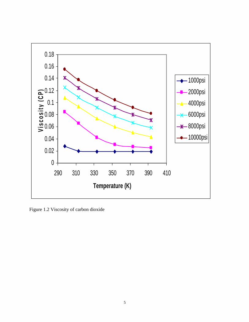
sweep efficiency. In a typical reservoir, temperature is usually between 80 and 250°F, and the
pressure will be kept over MMP, minimum miscibility pressure, Figure 1.1[3] At these
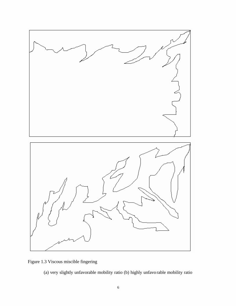
conditions, the CO2 has viscosity around 0.06cp, Figure 1.2. The reservoir oil has viscosity
between 0.1 and 50 cp. This viscosity ratio leads to a mobility ratio,
MK KCO
CO
oil
oil=
2
2µ µ
which is greater than unity, because the permeability of CO2 and oil are comparable in
magnitude. This unfavorable mobility ratio contributes to “miscible viscous fingering”, Figure
1.3. As a result, CO2 bypasses much of the oil in the reservoir, which reducing the areal sweep
efficiency. Low viscosity of CO2 also contributes to the low vertical sweep efficiency, especially
in stratified reservoirs. The highly mobile CO2 enter the most permeable zones, and the oil

3
residing in the low permeable zones cannot be efficiently displaced. Although the injection of
large volumes of CO2 will eventually lead to improved sweep efficiency, an increase in CO2
viscosity would result in an increased rate of oil recovery. Therefore, an increase in the viscosity
of CO2 could substantially increase economics of the oil recovery project. It has been estimated
by US DOE National Petroleum Technology Office that if the viscosity of the CO2 could be
increased by a factor of 2-10, the resultant oil production would increase from the current level
of 180,000 barrels per day (about 3% of domestic oil production) to 400,000 barrels per day.
4
Figure 1.1 Minimum miscibility pressure (MMP) [3]
5
0
0.02
0.04
0.06
0.08
0.1
0.12
0.14
0.16
0.18
290 310 330 350 370 390 410
Temperature (K)
Visc
osit
y (C
P)
1000psi
2000psi
4000psi
6000psi
8000psi
10000psi
Figure 1.2 Viscosity of carbon dioxide
6
Figure 1.3 Viscous miscible fingering
(a) very slightly unfavorable mobility ratio (b) highly unfavorable mobility ratio
7
1.2 CO2 for Formation Fracturing
Besides EOR, liquid CO2 is also widely used in fracturing formation as a proppant carrier
for sand fracturing. In this process, cold CO2 (-20°C) is delivered to a well site using tanker
trucks. Liquid CO2 is then rapidly injected into the tight gas formation, generating elevated
pressures. When this pressure (typically 5000~10000 psia) cause a vertical fracture to form
1/8~1/2” in width, a distinct pressure drop is observed at the wellhead. Sand is then slurried into
the CO2, and pumped into the fracture. Typically, the fracture collapses in less than one minute,
and the sand particles that flow into the fracture “prop” it open, providing a high permeability
flow path for the gas.
If the viscosity of CO2 could be increased, the efficiency of this process could be
increased in three ways: large proppant could be used, decreased leakoff of CO2 into the fracture
faces could occur, and an increased extent of the fracture would be achieved. The thickener
would cause skin damage as it precipitates when the CO2 is produced from the fracture.
8
2.0 BACKGROUND AND LITERATURE REVIEW
The high mobility of CO2 has a significant influence on flooding efficiency. Therefore,
much research has being done in order to increase the flooding efficiency. The only commonly
employed technique of CO2 mobility reduction is the water-alternating-gas technique, which
lowers CO2 mobility by reducing relative permeability to CO2 via increased water saturation.
CO2-foams (high volume fraction CO2 foams with continuous lamellae of aqueous surfactant
solutions) have such low mobility that they are used for profile modification (blocking high
permeability, watered-out zones). The mobility of these foams cannot be easily or reliably
controlled or moderated to the levels required for mobility control.
2.1 WAG
The use of the water-alternating-gas (WAG) procedure [4, 5] decreases the relative
permeability of CO2 by increasing the water saturation within the porous media. The main
advantage of this method is that both CO2 and water are inexpensive and readily available in
large volumes. However, this injection of large volumes of water prolongs the duration of the
CO2 flood. Further, there are concerns that the additional water in reservoir may shield residual
oil from CO2 flooding and increase the mass transfer resistance associated with the displacement.

9
2.2 Previous Attempts to Increase the Viscosity of CO2
2.2.1 Entrainers (cosolvents)
Llave and coworkers[6, 7] used entrainers (cosolvent s) to improve CO2 mobility control.
The definition of entrainer, based on this approach, is a chemical additive that enhances the
viscosity of CO2 and the solubility of crude oil components in the CO2-rich phase. The
cosolvents included n-decanol, ethoxylated alcohols, isooctane and 2-ethylhexanol. Even though
substantial viscosity increases were reached, large amounts of the entrainers were employed. For
example, viscosity increases of 243% were attained with isooctane and an increase of 1565%
was realized with 2-ethylhexanol. The entrainer concentrations of 13 mole% and 44 mole%,
respectively, were very high.
2.2.2 In- situ Polymerization of CO2 Soluble Monomers
Terry and coworkers[8] attempted to increase CO2 viscosity by in-situ polymerization of
monomers miscible with CO2. The polymerization is carried out while the monomer (solute) is in
the CO2 supercritical phase (solvent). The polymerizations were successfully carried out at
approximately 160°F and 1800 psi, the temperature and pressure are typical for oil reservoirs in
which CO2 is applied as a miscible fluid. The apparatus used for polymerization also allowed the
measurement of the viscosity of the resultant CO2/polymer system. However, even though the
polymers were made successfully, no apparent viscosity increases were detected because the
polymers were CO2-insoluble and precipitated during the reaction.

10
Lancaster and coworkers also tried in-situ “polymerization”, a reaction between organic
titanates with organic substrates, which include pyroga llol, resorcinol, silicic acid, phenol,
hydroquinone.[9, 10] A fast reaction did take place between organic substrate and titanate, but the
products were completely insoluble in liquid CO2. Noting the gelation of diesel oil after the
interaction of an amine with gaseous CO2 in diesel, they also hoped the reaction products of
liquid CO2 and mono n-butylamine would be soluble in liquid CO2. The product was CO2-
insoluble, however.
2.2.3 Small, Associating Compounds
Heller and coworkers considered organometallic compounds as CO2 viscosifiers. [11, 12]
They studied the solubility of organotin fluorides in various solvents including dense CO2. The
trialkyltin fluorides have structure R3SnF, and associate in the form of a penta co-ordinate
species. R represents alkyl, alkylaryl, or aryl group. Because of electronegativity differences
between tin and fluorine atoms, there exist dipole moment in these molecules, which cause weak
dipole-dipole interactions between adjacent molecules. Even at low concentrations (less than
1wt%), this transient polymer can increase the viscosity of non-polar solvents by several orders
of magnitude. Tri-n-butyltin fluoride is a representative example of these organometallic
viscosifiers. Although these polymers viscosified liquefied petroleum gas, they did not thicken
CO2 due to their low CO2 solubility.
The research in University of Pittsburgh began with surfactants, which contain a
hydrophilic and hydrophobic functional group. None of 70 commercially available surfactants
were soluble in CO2. Secondly, tributyltin fluoride, a well-known alkane-gelling agent in CO2

11
was investigated. Although it was able to increase the CO2 viscosity by several orders or
magnitude in low concentration, very large amounts of pentane cosolvent were required.
Polyfluoroether oils were also investigated. They all easily dissolved in liquid CO2 at relatively
low pressures, but no significant viscosity increase was detected, even at concentrations of 5-10
wt%.
Recently, a modified semifluorinated trialkyltin fluoride was evaluated as a direct CO2
thickener. Carbon dioxide solubility was enhanced by introducing the fluoroalkyl functionality
into the trialkyltin fluoride molecular structure. Tris(2-perfluorobutyl ethyl)tin fluoride was
highly soluble in liquid CO2 at moderate pressure. The solution viscosity was raised by only 3.3
times at a concentration of 4wt% with this low molecular weight compound, however. This
modest viscosity increase was attributed to strong solute-solvent interactions and/or competition
between the fluoroalkyl fluorine and the fluorine bonded to the tin for association with tin of the
adjacent molecule.
Fluoroalkyl aspartate bisureas and ureas were synthesized and evaluated as potential CO2
thickener. All samples were soluble in CO2 at pressure below 7000psi, and temperature below
100°C. The fluoroether bisureas and ureas were more soluble in CO2 than fluoroalkyl bisureas
and ureas, because the fluoroether functionality was more CO2-philic than fluoroalkyl
funcitonality. However, of all of ureas which were soluble in CO2 at room temperature and
pressure below 5,000psi, none increased the solution viscosity significantly.
12
2.2.4 Dissolution of Conventional Polymers into CO2
A polymeric direct CO2 thickener must be soluble enough in CO2 at reservoir conditions
that it can induce an increase in viscosity. Ideally, the thickener can increase viscosity 2-10 times
in concentration of 1wt% or less.
Heller and coworkers at the NMIMT tested about 40 commercially available polymers.
They found only about 30% of these polymers were slightly soluble in dense CO2. In general,
these were also soluble in light hydrocarbons and were completely insoluble in water. These oil-
soluble polymers are mostly based on straight-chain hydrocarbons, with low molecular weight,
and are atactic in their molecular structure. However, none of these polymers were able to
increase the viscosity of the resulting solution, because their MW and/or solubility in CO2 were
too low.
Heller and coworkers then synthesized poly-α-olefins. The method comprised of the
synthesis of homo-, co-, and ter-polymers of various α-olefins(1-olefins) in the C5 to C12 range.
The goal was to synthesize amorphous and atactic polymers of varying molecular weights and
with side chains, which vary in carbon numbers. The aim was to synthesize a polymer with high
entropy from irregularity and disorder, which would cause it to be easily dissolved in dense CO2.
They studied the Ziegler-Natta catalysts, the reaction conditions, and the effect on the structure.
The results were not promising, as these polymers did not induce a significant viscosity increase
due to their low CO2-solubility.
Heller and coworkers also considered telechelic ionomers. Ionomers are hydrocarbon
polymers containing relatively few ionic groups pendent to a hydrocarbon polymer chain. They
studied the possibility of using hydrocarbon-based telechelic ionomer as an effective thickener
13
for dense carbon dioxide in their evaluation of sulfonated polyisobutylene.[13] Due to its low
solubility in dense CO2, the ionomer did not enhance the viscosity of CO2 substantially.
Lancaster and coworkers[9, 10] also tried to increase the liquid CO2 viscosity via polymer
addition. They considered caprolactone polymers including either aliphatic alcohol or methoxy
acetic acid terminations, and the others were copolymer condensate products of caprolactone and
ethyleneimine. All polymers were insoluble in liquid CO2, and precipitated out of solution as
solids or oils.
Davis, Irani and coworkers[14-18] found a series of polymers which were useful in
increasing the viscosity of carbon dioxide. The polymers included polysilylenesiloxane,
polysilalkylenesilane, polyalkylsilsesquioxane and polydialkylsilalkylene polymers. An
extensive experimental program identified a number of polymer types that could be dissolved in
CO2 with the addition of cosolvents. They also studied suitable types of polymers and
cosolvents[19] They also investigated the CO2 flooding process in laboratory, using a sight glass
for solubility measurements and a core flood apparatus for mobility measurement. In their core
testing, oil recovery tests were also performed. Oil recovery was accelerated and CO2
breakthrough was delayed with viscosified CO2. The displacement efficiency was improved over
regular CO2 flooding. The disadvantage of their method is it required a significant amount of
cosolvent (e.g. 15% toluene) to dissolve a high molecular weight silicone polymer capable of
increasing the viscosity of carbon dioxide.
DeSimone and coworkers[20, 21] found amorphous (or low melting) fluoropolymers and
silicones are soluble in CO2 at readily accessible conditions(T<100C and P<450bar). These
soluble polymeric materials are termed as CO2-philic. They synthesized poly(1, 1-
dihydroperfluorooctyl acrylate)(PFOA), Mw~1.4*10(6), with free radical synthesis. PFOA was

14
synthesized in supercritical CO2, with AIBN initiator. The visual cloud point is 220 bar for 3.7
w/v%. The viscosity result indicated that PFOA significantly increased the CO2 viscosity. CO2
solutions with 3.7w/v% and 6.7w/v% PFOA have viscosity 0.25cp and 0.55cp in 360bar,
respectively, while the viscosity of neat CO2 is about 0.1cp. This was the first reported viscosity
enhancement of CO2 without the use of a cosolvent. Although the degree of thickening at dilute
concentrations was not as substantial as desired for EOR, this work demonstrated that CO2
thickeners could be made by designing the thickener specifically for dissolution in CO2.
Enick and coworkers also evaluated fluorinated telechelic disulfate, by introducing CO2-
philic fluoroether functionality into the structure of polyurethane telechelic disulfate. The
compound was highly soluble in liquid CO2 at pressure lower than 7000psi. There existed an
optimal molecular weight of about 19000, where the fluorinated disulfate exhibited the highest
solubility in CO2. Below this molecular weight, the CO2-philic fluoroether content diminished
and the disulfate became more polar and the CO2-solubility decreased. As the molecular weight
increases above 19000, the effect of unfavorable entropy of mixing decreases the solubility in
CO2. The CO2-phobic disulfate end groups promoted intermolecular association in CO2
environment more effectively than high molecular weight CO2-soluble polymers. These
relatively low molecular weight ionomers were more effective than high molecular weight
random polymers, such as poly(heptadecafluorodecyl acrylate), in solution viscosity increase at
comparable weight concentrations. The increases in viscosity were only 2-3 fold at concentration
up to 5wt%, were still not significant enough for EOR applications.
Fluorinated asparate methacrylate urea/ fluoroacrylate copolymers were synthesized and
evaluated as potential CO2 thickener. The concentration and the composition of the copolymer
have significant effect on the polymer solubility and solution viscosity. A CO2-philic

15
functionality such as fluroacrylate was necessary to impart CO2 solubility of the polymer; on the
other hand, the content of hydrogen bonding functionality was required in order to increase the
solution viscosity. The copolymer with an acryl/urea molar ratio of 19.5 was able to increase
solution viscosity by 9 times at 5wt%.
2.3 Solubility of Polymers and Copolymers in Supercritical CO2
In order to use a polymer or copolymer as a direct thicker for CO2 viscosity, it must be
designed to dissolve in CO2. Carbon dioxide is a good solvent for a variety of polymer and
copolymers. McHugh and coworkers have shown that CO2 can easily dissolve polymeric oils,
such as polydimethylsilicone, polyphenylmethylsilicone, perfluoroalkylpolyethers, and chloro-
and bromotrifluoroethylene polymers.[22, 23] In general, many investigators have confirmed that
the most CO2-philic polymers are fluorinated or silicone-based. Carbon dioxide is a feeble
solvent for nearly all other types of hydrocarbon-based polymers. Nonetheless, a significant
effort has been made to identify classes of commercial polymers that can dissolve in carbon
dioxide.
Heller and coworkers extensively tested many hydrocarbon-based polymers. The
polymers they found to be soluble at least in parts-per-thousand range in dense CO2 at 25°C
included polyα-decene, polybutene atactic, polyisobutylene, polyvinylethylether,
polymethyloxirane atactic. They also listed the polymers that are insoluble in CO2.[11] They found
that even the most soluble polymer polyα-decene, its solubility is less than 1wt% at pressure of
2900psi. Even though their initial goal was to find a polymer with viscosity increase ratios of
20~30, the best polymers they found showed values of this parameter of less than 1.3. Although
16
no viscosity enhancing polymer was identified, hydrocarbon-based polymers that exhibited slight
solubility in CO2 had solubility parameters less than 8 (cal/cm3)0.5. Ghenciu calculated the
solubility parameters in his PhD dissertation, and the solubility parameter of liquid CO2 is found
to be in the range of 4 to 5 (cal/cm3)0.5 at 298K and pressure above 10MPa.[24]
McHugh and coworkers investigated the solubility of poly(acrylates) in CO2 at
temperature and pressure up to 270°C and 3000bar, respectively.[25] The poly(acrylates) includes
methyl, ethyl, propyl, butyl, ethylhexyl, octadecyl. They also studied the random copolymer of
poly(ethylene-co-methyl acrylate), poly(tetra fluoro ethylene-co-hexa fluoro propylene). They
found that CO2 could not dissolve polyethylene, poly(acrylic acid), poly(methyl methacrylate),
poly(ethyl methacrylate), polystyrene, poly(vinyl fluoride), poly(vinylidene fluoride) at their
experimental working condition. Polyacrylates were found to exhibit solubility in carbon
dioxide, but at pressures an order-of-magnitude or greater than that associated with EOR. For
example, the cloud point pressure of poly(methyl acrylate) varied from 2500 bar at 25°C to 1600
bar at 200°C. They also found poly(vinyl acetate) was the most carbon dioxide soluble non-
fluorous polymer they detected, even though it has the same chemical formula as poly(methyl
acrylate), it was much more carbon dioxide soluble than poly(methyl acrylate).
Beckman and coworkers found non-fluorous polymers with very high solubility in
supercritical CO2.[26] Addition of only one Lewis base group (carbonyl) to a polyether can
significantly lower miscibility pressure in CO2, an ether-carbonate copolymer will dissolve in
CO2 at lower pressures than that of fluorinated polyether with a comparable number of repeat
units.
Johnston and coworkers also studied the solubility of homopolymers and copolymers in
carbon dioxide.[27] The cloud points of various polyether, polyacrylate, and polysilocane

17
homopolymers and a variety of commercially available block copolymers were measured at CO2
from 25-65°C and pressure from 1000 to 6000psi. They found the decreasing solubility in the
following order for the series: polyfluorooctylacrylate > polypropylene oxide >
polydimethylsilocane > polyethylene oxide > polyacrylates, where, the solubility of
polyfluorooctylacrylate is greater than 10wt%, while the polyacrylate is insoluble in the above
condition. They related the polymer solubility with the polymer-polymer interaction and surface
tension.
McHugh and coworkers studied a series of polyacrylate and poly (vinyl acetate)
(PVAc).[25] The cloud point pressure data at a concentration of 5wt% polymer, polyacrylate and
poly vinyl acetate were studied together. PVAc is much more soluble than poly methyl acrylate,
even the molecular weight of PVAc is 125000, which is much larger than the molecular of PMA,
which is only 31000. The experiment also found PVAc and PMA’s cloud point pressure respond
differently to the temperature change, at temperature range from 295K to 423K. The cloud point
pressure of PMA decreased as the temperature increased, while PVAc’s cloud point pressure
increased as the temperature increased. Even so, the PVAc’s cloud point pressure always much
lower than PMA’s cloud point pressure. McHugh and coworkers noticed the glass transition
temperature of PVAc is 21K higher than that of PMA, which indicated that the stronger polar
interactions between acetate groups relative to methyl acrylate groups. PVAc is considered to be
more polar than PMA, which helps the formation of a weak association of carbon dioxide and
vinyl acetate especially at moderate temperature. [25]
McHugh and coworkers studied poly(lactide) (PLA), which has been shown to dissolve
at high concentration in neat CO2.[28] The pressure required to dissolve PLA is higher than that to
dissolve PVAc. For PVAc and PLA at 5wt% concentration in CO2, the required pressure is

18
70MPa for PVAc, and 140MPa for PLA. Both PVAc and PLA are at 308K condition, and
molecular weight (Mw) is about 130000. Because the glycolide functionality are even less CO2-
philie than PLA, the copolymer of lactide and glycolide are even more difficult to dissolve in
CO2.
19
3.0 APPROACH
The proposed approach is to increase viscosity of CO2 by addition of dilute concentration
of a copolymer. To reach this goal, we propose to design and synthesize associating copolymers.
The ideal copolymer has two characteristics. The copolymer must contain CO2-philic groups
capable of making the polymer soluble in dense carbon dioxide. The polymer must also contain
CO2-phobic functional groups, which increase the viscosity of CO2 via viscosity-enhancing
intermolecular interactions while not dramatically reducing CO2 solubility.
The specific goal is to increase the viscosity of liquid CO2 by a factor of 2-10 in
concentration as low as 0.1~1wt%, as determined by Darcy’s Law for fluids the low Re flow of
through porous media. Fluorinated copolymers were initially evaluated in proof-of concept tests.
Non-fluorous polymers were then assessed in an attempt to identify an inexpensive non-fluorous
homopolymer that could be subsequently modified to become thickening agents.
3.1 Fluorous CO2 Thickener
Because the high solubility of fluoroacrylate polymers, it is the first choice in our search
for the CO2 thickeners. Although a high molecular weight polyfluoroalkylacrylate homopolymer
could induce a slight increase in CO2 viscosity, incorporation of the associating group into it can
dramatically increase the CO2 solution viscosity via intermolecular interactions. From all the
CO2 thickeners we investigated, we have found that the fluoroacrylate/styrene copolymer is a
promising candidate for thickening carbon dioxide. The fluoroacrylate functionality is highly
CO2-philic, thereby enhancing the copolymer solubility. The styrene is the CO2-phobic
20
viscosity-enhancing component. The intermolecular “stacking” of the CO2-phobic phenyl
groups can lead to the formation of macromolecular structures in solution.
The copolymer was bulk-polymerized, rather than solution-polymerized, to attain high
molecular weight. There is an optimal composition of the fluoroacrylate-styrene copolymer for
thickening carbon dioxide. The 29mol% styrene/71mol% fluoroacrylate was particularly
effective in thickening carbon dioxide as observed in falling cylinder viscosity tests. Higher
styrene content not only led to significant increases in the cloud point pressure, but also a
diminished thickening capacity. It is conjectured that the decrease in thickening may be
attributed to the increased intramolecular, rather than intermolecular stacking of the phenyl
groups.
We conducted a thorough rheological study of CO2 solutions containing up to 5wt% of
the 29mol%Styrene-71mol%Fluoroacrylate copolymer. This is accomplished with a falling
cylinder viscometer with aluminum cylinders of varying diameter. This enables the viscosity-
shear rate relationship to be determined. The mobility of thickened carbon dioxide solutions
flowing through Berea sandstone is also evaluated. Superficial velocities associated with EOR,
1ft/day and 10ft/day, are used, and increases in viscosity are reflected by increases in pressure
drop across the core at a specified flow rate.
3.2 Non- fluorous CO2 Thickeners
The fluoroacrylate-styrene copolymer was a proof-of-concept copolymer; it is not a
feasible candidate for CO2 thickening in the oil field because of the expense and environmental
persistence associated with its fluorine content. Therefore, we also initiated the design of non-

21
fluorous CO2 thickeners. The strategy was that we first try to identify highly carbon dioxide
soluble polymers that could be later functionalized with CO2-phobic associating groups. Several
promising non-fluorous CO2 soluble polymers were identified in the literature, including
poly(propylene oxide) and poly(vinyl acetate).
Beckman and coworkers have designed and synthesized several CO2-philic hydrocarbon
copolymers composed of (A) monomer 1 (M1) that contributes to high flexibility, high free
volume, and weak solute/solute interaction (low cohesive energy density or surface tension),
usually M1 shows low Tg, resulting a favorable entropy of mixing for the copolymer as well as
weak solute-solute interaction, easing dissolution into CO2. (B) monomer 2 (M2) that provides
specific solute/solvent interaction interactions between the polymer and CO2, through a Lewis
base group in the polymer structure.
Under this guideline, Oxirane/CO2 copolymers were synthesized, with sterically hindered
aluminum catalysts. This is done by copolymerizing propylene oxide (PO), ethylene oxide (EO),
or cyclohexene oxide (CHO) with CO2, incorporating the carbonyl groups into the backbone of
polymer. They found PO-CO2 copolymer with 56% carbonate was less CO2-philic than a
homopolymer of PO, but copolymer with 40% carbonate exhibited miscibility pressures lower
than that of the homopolymer. PO-CO2 copolymer also appeared to be more CO2-philic than
fluoroether polymers. CHO-CO2 with high chain lengths and a low amount of carbonate units
also exhibited very low miscibility pressures in carbon dioxide.[29]
Guided by such promising results, we decided to investigate the polybutadiene, and all its
derivatives. We can buy polybutadiene from Aldrich with different Mw and Mn. We also
invesitigated the hydroxylate ended polybutadiene, and acetate ended polybutadiene, because
butadiene is a good candidate for M1, and with low CED, low Tg, high flexiblility and high free

22
volume. While the acetate group is good associating group, combing them together, it may
produce a good CO2 thickener.
3.3 Non- fluorous Homopolymer
In our search for a non-fluorous homopolymer, we need to identify a good base-
homopolymer, upon which we incorporate associating groups, make copolymer a good CO2
thickener. In synthesizing a homopolymer, two characteristics must be attained. First, a CO2-
philic component that increases polymer solubility must be found. Second, there must be an
intermolecular associating component that increases solutions viscosity.
The polymers were chosen for synthesis based on their structure and attached groups. The
homopolymers were polybutoxyethyl acrylate, PBEA; polyethoxyethyl acrylate, PEEA;
polyvinyl ester and polyvinyl acetate. Both PBEA and PEEA were chosen based on their acrylate
group. Polyacrylates have been found to be CO2 soluble because of enhanced interactions
between carbonyl moieties. Polyvinyl ester has methyl substitutions making its structure similar
to that of Polypropylene oxide. In Polypropylene oxide’s case, the methyl substitution on each
monomer unit in the chain has a large effect on the solubility. Polypropylene oxide is also CO2
soluble because of the weak physical segments due to sterical effects and acid-base interactions
not being as prevalent. The reason polypropylene oxide is the guide for finding a CO2 thickener
is that polypropylene oxide is the best commercial base material up to date. The better the base
the more CO2-philic a polymer will be. The promising polymer, Polyvinyl acetate has already
been found to be CO2 soluble, but at a high molecular weight. The objective is to determine
whether or not polyvinyl acetate can be synthesized at a low molecular weight, using a more
23
accurate method of polymerization, Atom Transfer by Radical Polymerization (ATRP). If a low
molecular weight is achieved, then we need to find out whether its CO2 solubility is comparable
to the CO2 solubility of Polypropylene oxide.
In summary, the fluoroacrylate-styrene bulk-polymerized random copolymer has
exhibited the most promise as a CO2 thickener. Therefore, a rheological investigation of CO2-
fluoroacrylate-styrene copolymer solutions over a range of flow rates and concentrations was
conducted with a falling cylinder viscometry and with a flow-through-porous-media viscometer.
Also, to be environmental benign, and feasible in the oil fields, we have been designing and
synthesizing different non-fluorous polymers, mainly in acrylate-based and acetate-based
polymers.

24
4.0 THICKENING CANDIDATE S
4.1 Fluoroacrylate- styrene Copolymer
Among all the thickeners we tested, fluoroacrylate-styrene copolymer
(heptadecafluoroacrylate styrene copolymer) has the most significant viscosity enhancement.
The fluoroacrylate functionality is highly CO2-philic, while the intermolecular "π-π stacking" of
the CO2-phobic phenyl groups associated with the styrene monomer leads to the formation of
macromolecular structures in solution.[30]
4.1.1 Material and Methods
Both styrene and 3,3,4,4,5,5,6,6,7,7,8,8,9,9,10,10,10-heptadecafluorodecyl acrylate
(HFDA) were purchased from Aldrich. The styrene was distilled under vacuum before use. The
heptadecafluorodecyl acrylate and styrene were passed over inhibitor removal columns to
facilitate copolymerization. All other solvents and reagents were received from Aldrich, and
used without purification.
The polymerization technique is bulk free radical polymerization, with AIBN as initiator.
The amount of initiator is about 0.2% mole of monomer. The reaction occurs in a 50 ml glass
ampule, in an inert N2 atmosphere. Specified amounts of HFDA, styrene and AIBN are charged
into the ampule. The ampule is sealed and placed in a water bath at 65°C for 12 hours. The
reaction products are then dissolved in 1,1,2-trichlorotrifluoroethane. The copolymer is then
precipitated in methanol (which is capable of dissolving both monomers, but not the copolymer),

25
washed several times and dried under vacuum. The structure of the copolymer, Figure 4.1, is
characterized using Mattson FT-IR and Bruker 300MHz NMR.
O
O
(CF2)7CF3
+AIBN
338K
O
(CF2)7CF3
) ( )( x y
O
StyreneIntermolecularAssociating Component Copolymer
FluoroacrylateCO2-Philic Component
Figure 4.1 Synthesis of the Fluoroacrylate-Styrene Random Copolymer
4.1.2 3M Fluoroacrylate Styrene Copolymer
The Aldrich fluoroacrylate is not commercially available in large amount. Therefore, A
3M fluoroacrylate with C6~C10 fluoroalkyl side chains was also evaluated. 3M produces tons of
this monomer each year. We used the same free radical polymerization technique to generate
copolymers based on the 3M fluoroalkylacrylate monomer.

26
4.1.3 Random Styrene - FA- x Copolymer
We also tried to synthesize random copolymer of styrene and the Asahi FA-x fluorinated
monomer. FA-x is 2-perfluoroalkyl (C6-C16) ethyl acrylate, which is about 10 times cheaper
than the Aldrich monomer. We examined both the homopolymer of FA-x and random
copolymers of FA-x and styrene.
The synthesis of random Copolymer of FA-x and styrene is similar to the synthesis of
fluoroacrylate-styrene copolymer, substituting HFDA with FA-x. We only need to purify the FA-
x before use. First, FA-x is washed with 5% NaOH three times, it is washed with distilled water
three times, MgSO4 is added to remove the trace water, then it was put into refrigerator, and then
filtered. The synthesis of FA-x homopolymer is the same as the synthesis of copolymer, only use
FA-x as monomer, instead of FA-x and styrene.
4.2 Butadiene - Acetate Copolymers
An attempt was also made to synthesize a non-fluorous copolymer composed of two
monomers, designed as M1 and M2. M1 is selected from groups that have low cohesive energy,
while M2 group should exhibit an intermolecular association with CO2.
Polybutadiene has low Tg of about 170K. It is a good candidate as M1 for its low
cohesive energy density. Several butadiene-M2 copolymers were studied. M2 can be one of
many types of monomer, as long as it has some kind of association with CO2, such as Lewis base
groups, ethers and acetates. Acetate is a good candidate for M2, forming a carbonyl structure in
side chain. Because it is difficult to directly co-polymerize butadiene and acetate, the synthesis
27
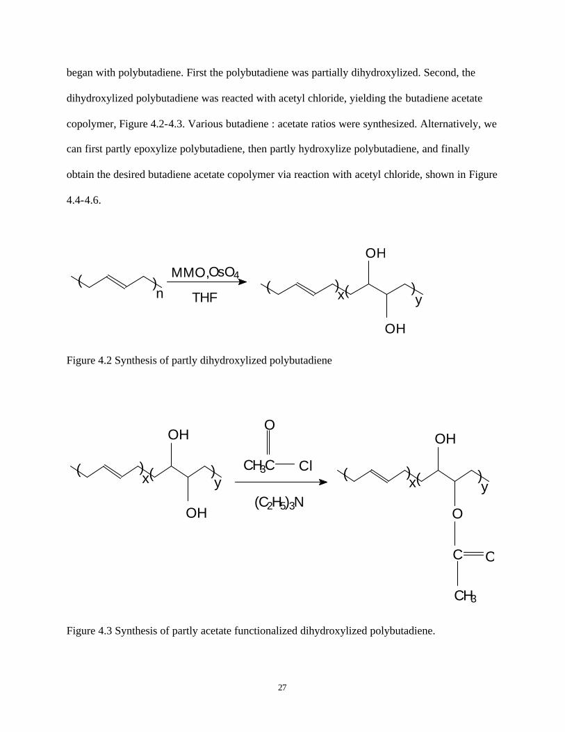
began with polybutadiene. First the polybutadiene was partially dihydroxylized. Second, the
dihydroxylized polybutadiene was reacted with acetyl chloride, yielding the butadiene acetate
copolymer, Figure 4.2-4.3. Various butadiene : acetate ratios were synthesized. Alternatively, we
can first partly epoxylize polybutadiene, then partly hydroxylize polybutadiene, and finally
obtain the desired butadiene acetate copolymer via reaction with acetyl chloride, shown in Figure
4.4-4.6.
( )THF
MMO, OsO4( ) )(x y
OH
OH
n
Figure 4.2 Synthesis of partly dihydroxylized polybutadiene
( ) )(x y
OH
OH
O
ClCH3C
OH
yx( ))(
O
C O
CH3
(C2H5)3N
Figure 4.3 Synthesis of partly acetate functionalized dihydroxylized polybutadiene.

28
( )
O
( )
C OOH
O
x y( )
n
Figure 4.4 Synthesis of partly epoxylized polybutadiene
O
( )( )( ) ( )x
xy
yOH
LiAlH4
THF
Figure 4.5 Synthesis of partly hydroxylized polybutadiene
CH3C
O
ClO
C O
CH3
( )( ) ( ) ( )x xy y
(C2H5)3N
OH
Figure 4.6 Synthesis of partly acetated polybutadiene
29
4.3 Other Non- fluorous Polymers
In an attempt to identify an inexpensive highly CO2-soluble polymer (that could
subsequently be modified into a thickener), many non-fluorous polymers were evaluated,
including poly propylene oxide, polyethoxyethyl acrylate, polybutoxyethyl acrylate, polyvinyl
ester, poly vinyl acetate, polymethyl acrylate and poly vinyl formate. Among them, the poly
vinyl acetate and low molecular weight poly (propylene oxide) exhibited appreciable CO2
solubility in our apparatus (rated to 7000psia).
4.3.1 Materials and Methods
All the monomers, solvents and reactants were purchased from Aldrich Chemical Co.
Monomers were purified using an inhibitor removal column.
The first method of synthesis, free radical polymerization using azobisisobutyronitrile
(AIBN), had the monomer and AIBN mix together in an ample. They were degassed with N2 for
ten minutes and sealed. Then the ample was heated in a silicon oil bath for three hours at 60° C.
The solubility of the sample was tested with a number of different solvents, including,
tetrahydrofuran (THF), methane, and hexane. Then the polymer was precipitated using a solvent
that it was very insoluble in. Three purification cycles were done using the Rotavaporator and
THF, to clean the polymer and remove any excess monomer. Finally the purified polymer was
dried in a vacuum oven for 24 hours.
30
The second method of synthesis was Atomic Transfer by Radical Polymerization
(ATRP). Although ATRP was used for all homopolymers, two different types of purification
methods were used.[31, 32] For example, the application of ATRP to the homopolymerization of 2-
hydroxyethyl acrylate was previously reported.[31] It was determined that through ATRP the
polymerizations exhibit first order kinetics and the molecular weights increase linearly. In
addition, the polydispersities remain low throughout the polymerization. For polybutoxyethyl
acrylate, polyethoxyethyl acrylate, polyvinyl ester, ATRP was done using following reactants:
Monomer, Initiator: Methyl 2-bromopropionate, Catalyst: CuBr, and Ligand : 2-2’ bipryidine
with ratios M:I:Cu:L = 50:1:1:2. These reactants were added to the ample and degassed for ten
minutes with N2. The ample was sealed and placed in the oil bath for three hours at 90° C. The
second ATRP method was used in order to try to control the molecular weight of polyvinyl
acetate. Synthesis was done using the following reactants: Monomer, Initiator: CCl4, Catalyst:
FeAc2 and Ligand: N, N,N’N’’,N’’-pentamethyldiethylenetriamine (PMETA) with ratios M:I: C:
L=15:1:1:1. Three freeze-pump-thaw cycles were performed and the flask was sealed under the
vacuum and placed in the oil bath for three hours at 60° C. The polymer was purified through an
Al2O3 column. It was washed twice with THF and then dried in a desiccator overnight.
4.3.2 Characterization
The weight average Mw, number average Mn, and polydispersity index were
evaluated using Gel Permeation Chromatography (GPC). GPC separates molecules in
solution by their effective size in solution. In this project, the sample had to be soluble in
THF in order to be analyzed, because THF had been selected as the sole solvent to be used in
31
the GPC. Once inside the GPC, the dissolved resin is injected into a continually flowing
stream of solvent. The solvent, mobile phase flows through highly porous, rigid particles
(stationary phase) tightly packed together in a column. The sizes of the particles pores are
controlled and available in a range of sizes. The distribution of chain lengths and therefore
molecular weight of the polymer are dependent on the method of synthesis. A free radical
polymerization, for example, may produce a polymer with a very broad distribution of chain
lengths and high molecular weights. The molecular weights of the THF-insoluble fluorinated
copolymer were determined by American Polymer Standards Corporation. This company
employed fluorous solvents in their GPC.

32
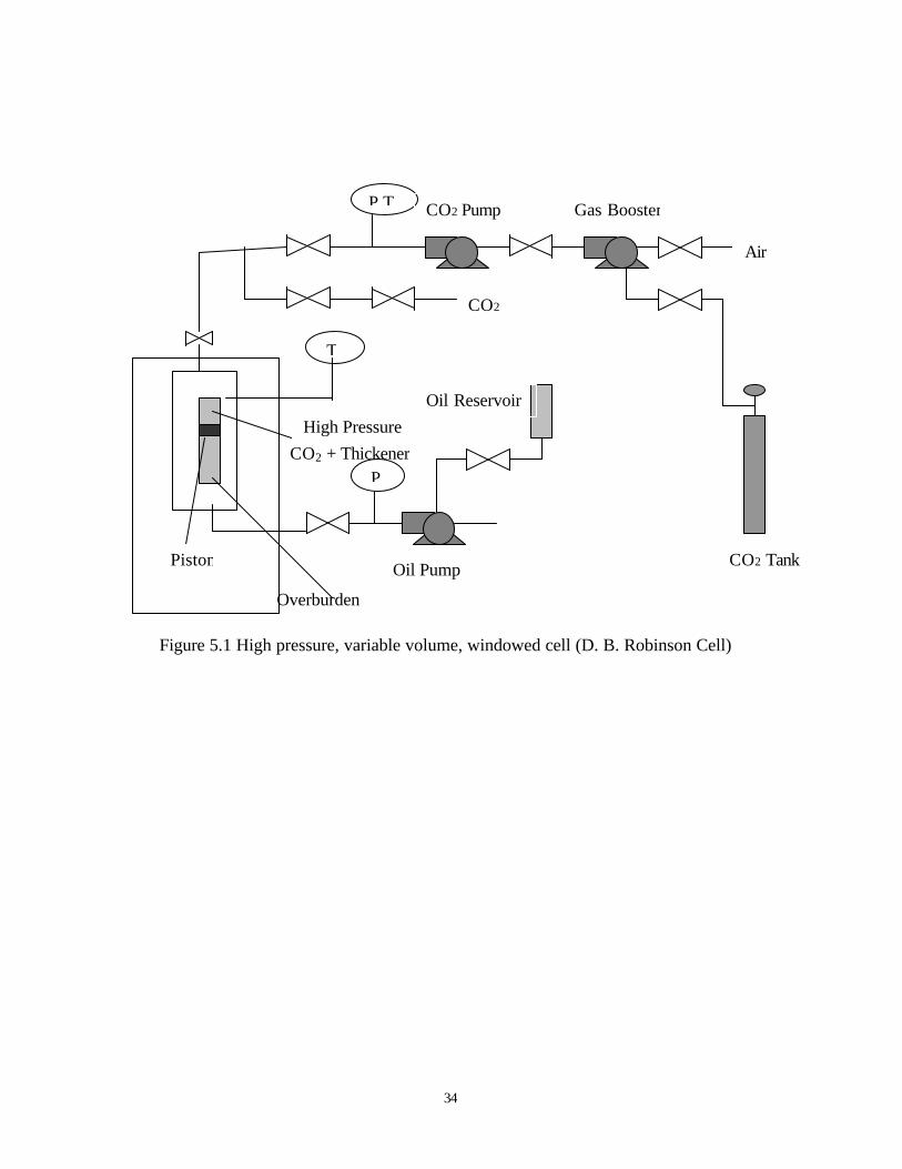
5.0 SOLUBILITY APPARATUS
The phase behavior studies of our CO2 thickeners are performed at room temperature,
using a high pressure, variable-volume, windowed cell (D. B. Robinson Cell), with a cylindrical
sample volume, as Figure 5.1. The system is rated to 7000psi and 180°C.
Isothermal compression and expansions of sample/CO2 mixtures of specified overall
composition are used to determine polymer solubility via cloud point determination. The
procedure is as follows. First, the CO2 thickener sample is added into the sample chamber along
with several stainless steel mixing balls. Then high-pressure carbon dioxide is displaced into the
positive displacement pump with a gas booster. The carbon dioxide liquid is then injected into
the sample volume by a positive displacement pump as the sample volume is expanded at the
same volumetric rate via the withdrawal of the overburden oil. Therefore, one can add a desired
amount of liquid carbon dioxide into the sample volume in a well-controlled, isothermal, isobaric
manner.
After the high-pressure carbon dioxide is injected into the sample volume, the inlet valve
to isolate the sample volume from high-pressure carbon dioxide is closed. The pressure of the
sample volume can be increased by pumping the overburden fluid into the windowed cell,
decreasing the sample volume. Mixing with the stainless steel balls is accomplished by rocking
the view-cell until the sample is totally dissolved. The pressure of the sample volume is reduced
by expanding the sample volume at the same time the overburden fluid is withdrawn at a high
flow rate, until visual observations of the initial appearance of a second phase occurred. Then the
sample volume pressure is increased and the cell rocked until a transparent solution is viewed
again. The overburden fluid is then withdrawn at a very low flow rate, providing a more

33
accurate cloud point pressure determination. This procedure is repeated several times, yielding
an average cloud point pressure. The cloud point pressure is the minimum pressure required to
keep the thickener dissolved in carbon dioxide. Below this pressure, the solution becomes a two-
phase system.
We can conduct cloud point experiment with different overall compositions. The results
can be presented in a pressure-composition diagram at the temperature of interest.
34
Figure 5.1 High pressure, variable volume, windowed cell (D. B. Robinson Cell)
P
P,T
T
High Pressure
Piston Oil Pump
Oil Reservoir
CO2 Tank
Air
Gas Booster CO2 Pump
CO2 Venting
CO2 + Thickener
Overburden Fluid

35
6. 0 FALLING CYLINDER VIS COMETER
The simplest and quickest test for estimating low pressure and high pressure fluid
viscosity is falling object viscometry. Beginning with Lawaczeck,[33] it has been widely studied
and applied in rheology studies.[30, 34-40]
Falling cylinder viscometer is also a useful tool for high pressure viscometry when a
relatively low viscosity single phase exists. Both petroleum engineering and chemical
engineering investigators have used various versions of falling object viscometers in their studies
of carbon dioxide-rich systems. [41, 42]
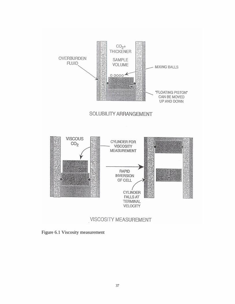
We used a thick-walled, precision, hollow glass tube as the viscometer [D.B. Robinson]
and a series of close clearance aluminum cylinders (Figure 5.1) for viscosity measurement. The
hollow glass tube is the same tube used in phase behavior studies. The falling cylinder
dimension is shown in Table 6-1.
For carbon dioxide or carbon dioxide-thickener solution viscosity measurements, the
following procedure is used. The aluminum cylinder is moved to the top of the vertical,
transparent tube, which is filled with the high pressure fluid, by rapidly inverting the cell. The
cylinder falls down. Because of the narrow annular gap bounded by the aluminum cylinder wall
and glass cylinder wall, the falling aluminum cylinder rapidly attains its terminal velocity.
Velocity is calculated be measuring the falling time between the distance of two locations,
Figure 6.1.
36
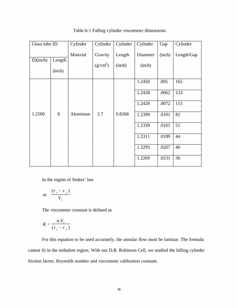
Table 6- 1 Falling cylinder viscometer dimensions
Glass tube ID
ID(inch) Length
(inch)
Cylinder
Material
Cylinder
Gravity
(g/cm3)
Cylinder
Length
(inch)
Cylinder
Diameter
(inch)
Gap
(inch)
Cylinder
Length/Gap
1.2450 .005 165
1.2438 .0062 133
1.2428 .0072 115
1.2399 .0101 82
1.2339 .0161 51
1.2311 .0189 44
1.2293 .0207 40
1.2500
8
Aluminum
2.7
0.8268
1.2269 .0231 36
In the region of Stokes’ law
µρ ρ
∝−( )c f
cV
The viscometer constant is defined as
KVc
c f
=−
µρ ρ
.( )
For this equation to be used accurately, the annular flow must be laminar. The formula
cannot fit in the turbulent region. With our D.B. Robinson Cell, we studied the falling cylinder
friction factor, Reynolds number and viscometer calibration constant.
37
Figure 6.1 Viscosity measurement

38
6.1 Friction Factor
The friction factor f is affected by the nature of the flow (laminar or turbulent),
contraction, expansion and imperfections in the hollow cylinder or falling cylinder. The
experiment calibration constant is usually smaller than theoretically calibration constant, owing
to contraction, expansion, and imperfection losses. Because these effects and the effect of
turbulence cannot be treated mathematically, dimensional analysis was used to develop a
correlation to account for these effects. The friction factor is
fFg Gc Ded V lf c
=4
2 2
. .. . . .π ρ
When only laminar flow occurs, the friction factor is: f = 16/NRe
Here, NDe Vc f
Re
. .=
ρ
µ, Reynolds number
Fg: force of gravity on the falling body, g-force
Gc: universal gravitational constant, g-mass-cm./g-force-sec2
De: equivalent diameter of the viscometer tube-body annulus, cm
De dDd
D dD d
= −−+
22 2
2 2. . ln
ρ f : fluid density, g/cm3
L: length of the falling cylinder, cm
Vc: terminal velocity of the falling cylinder, cm/s
µ : absolute viscosity, poise

39
1.E+00
1.E+02
1.E+04
1.E+06
1.E+08
1.E-06 1.E-04 1.E-02 1.E+00 1.E+02
Reynolds Number NRe
Fric
tion
Fact
or
Piston1.2438 CO2Piston1.2399 CO2 Piston1.2339 CO2Piston1.2438 Sam.Piston1.2399 Sam.Piston1.2339 Sam.f=16/NRe
Figure 6.2 Friction factor vs. Reynolds number
40
From our experiment data, in Figure 6.2, all our experiments, the slope of the line is
constant, and equal to –1, indicating all appreciable frictional effects are laminar. The difference
between our experiment lines and f = 16/NRe, are due to the contraction, expansion and
imperfection losses.
6.2 Reynolds Number
Lohrenz and coworkers[34, 35] studied calibration constants in laminar region and
calibration constants in turbulent region, they found the critical NRe is about 0.13 ~ 1.0. They
concluded that when the Reynolds number is close to 0.1, all frictional effects may be assumed
to be laminar.
From result of our data, the Reynolds number of most falling cylinder are between
0.1~1.0, for pure CO2. For the more viscous polymer solutions, the Reynolds number is expected
to be smaller.
6.3 Theoretical and Experimental Calibration Constants
We can assume that the neat CO2 solution or dilute polymer solution is Newtonian, so,
µρ ρ
=−
KVc
c f
Then, we can compare the experimental calibration constant K with the theoretical
calibration constant, ignoring the resistances because of non- ideal falling.

41
In our falling cylinder viscometer, we used neat CO2 as our fluid, at 297K and 3000psi.
Because both the density and viscosity of carbon dioxide are known at these conditions, the
calibration constant for a cylinder can be determined if the terminal velocity is measured.
KVc
c f
=−
µ
ρ ρ
We can also determine the theoretical calibration constant from the size of the falling
cylinder and the hollow cylinder:
Kr g
r J Kc
c=
−' '2
Where,
Jr r
rr
r rt cc
tt c
'( ) ln ( )
= −− + +
4
2 2 2 2
K
r r rr
rr
r rr
r r r rr
r
c t c
cc
t
t cc
tt c c
c
t
'
( )ln( )
ln( )( ) ln( )=
− − −
− + ++
21
1
2 2
2 2 2 2
In Figure 6.3, the diagonal line is the reference line if experimental calibration constant is
equal to theoretical calibration constant. The vertical line segment is theoretical “error bar”
associated with the machining tolerance of the falling cylinder surface, ±0.00015 inch difference
from the average of the diameter. The horizontal line segment is the experiment calibration
constant error associated with the range of terminal velocities measured for neat carbon dioxide.

42
The experimental calibration constant is reasonably close to the theoretical constant.
These results (which are typically not reported for high pressure viscometers) show that the
theoretical and experimental values of the viscometer constant agree to within 50%.
This difference may be attributed to imperfections in the aluminum cylinder, the absence
of hemispherical heads to the cylinders, non-coaxial descent of the cylinder and/or cylinder
rotation.

43
0
0.001
0.002
0.003
0 0.001 0.002 0.003
Experiment Calibration Constant K (cm3.s-2)
Th
eore
tica
l Co
nst
ant K
(cm
3 .s-2
) theory
Y=X
theory1
theory2
theory3
theory4
theory5
theory6
theory7
theory8
exp1
exp2
exp3
exp4
exp5
exp6
exp7
exp8
Glass Tube Inside Radius=1.588cmAluminum CylinderPure CO2
at 297K and 34MPa
1.2451.24381.24281.2399
1.2339
1.2311
1.2293
1.2269
Figure 6.3 Experiment calibration constant vs theoretical constant

44
7.0 FLOW-THROUGH-POROUS -MEDIA VISCOMETER
The most meaningful measure of carbon dioxide solution viscosity for EOR is
associated with the mobility of the fluid flowing through porous media at superficial
velocities comparable to those attained in petroleum reservoirs. The ability for thickened
carbon dioxide to flow through sandstone at flow rates that occur in the oil field is best
measured by displacing thickened carbon dioxide through sandstone cores at the
appropriate superficial velocity. A clean, homogeneous Berea sandstone core [American
Stone] is used to simulate the performance of CO2 flooding in a sandstone reservoir.
7.1 Experimental Apparatus
The neat or thickened carbon dioxide is prepared in the same manner as described
in the solubility experiments. The objective of the experiment is to displace a single
phase fluid through the sandstone core at a constant flow rate. The pressure of the
thickened carbon dioxide is maintained at a high enough pressure to ensure a single phase
of fluoroacrylate-styrene copolymer-carbon dioxide solution, for polymer concentrations
up to 2wt%.
Fluid viscosity can be determined with Darcy’s law for the flow of a Newtonian
fluid through porous media in the creeping flow regime.
∆ PL
vD
=.µ
45
Where, v is velocity of the fluid flow through the core, µ is absolute viscosity of the
fluid, D is permeability, and L is the length of the core. Experiments of neat carbon dioxide can
be performed to determine the permeability. Using this permeability value, the viscosity of
thickened carbon dioxide solutions can be determined simply by measuring pressure drop. The
pressure drop over distance is proportional to the fluid viscosity. Because the same core was
used for the viscosity of thickened CO2 to neat CO2, the ratio of the viscosity of thickened CO2
to neat CO2 was estimated as the ratio of the respective pressure drops along the length of the
core.
( )( ) 22 //
CO
olutioncopolymers
CO
olutioncopolymers
LPLP∆
∆=
µµ
In our experiments, Figure 7.1, the thickened carbon dioxide was prepared in the
Robinson cell while the porous media and tubing were charged with neat carbon dioxide. The
thickened carbon dioxide was then displaced from the sample volume toward the porous media.
The volume available for the core effluent was being expanded at the same volumetric rate that
thickened carbon dioxide entered the core, resulting in well-controlled, continuous flow through
the core. The pressure drop through the core was monitored continuously as the carbon dioxide
solution flowed through the core at a superficial velocity of either 1 or 10 ft/day, which are the
typical flow rates in the field. To study the very high flow rate effect on the thickening ability,
we also simulate the flow rate at 50 and 80ft/day.
All flow lines, internal volumes and pressure tap volumes for the differential pressure
transducers are kept to a minimum so that accurate flow data can be obtained. There are four
pressure taps, as shown in Figure 7.1, that enable the pressure drop along each third of the core

46
to be determined. This facilitates the detection of polymer retention at the entrance of the core,
which would be evidenced by a higher pressure drop in the first third of the core than the
pressure drops in the other two thirds.
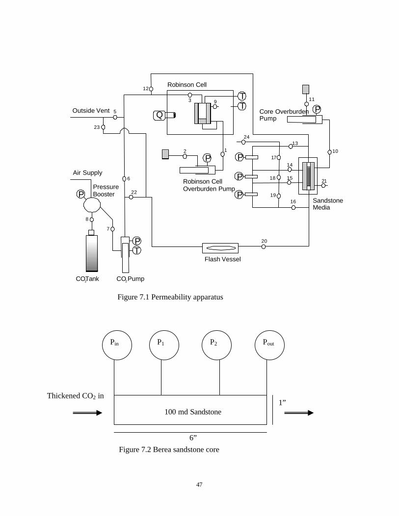
47
T
TT
P
P
P
P
P
P
P
COTank2
PressureBooster
CO Pump2
Robinson CellOverburden Pump
Core OverburdenPump
Flash Vessel
Robinson Cell
SandstoneMedia
Outside Vent
Air Supply
12
3
5
6
7
8
9
10
11
12
13
14
15
16
17
18
19
20
21
22
23
Q
24
Figure 7.1 Permeability apparatus
Thickened CO2 in
Figure 7.2 Berea sandstone core
100 md Sandstone
Pin P1 P2 Pout
1”
6”

48
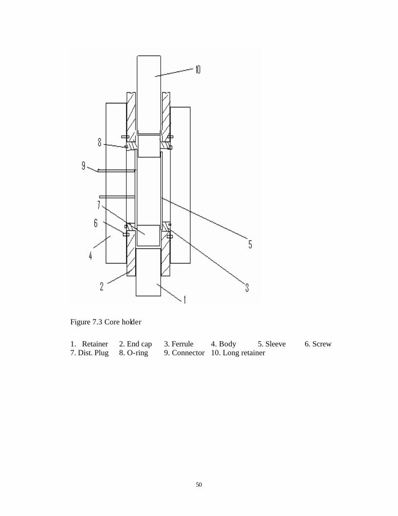
7.2 Berea Sandstone Core
Berea sandstone core is manufactured by American stone Co., produced from Cleveland
Quarries. The details of sandstone core are shown in Figure 7.2. The core has length of 6 inches
and roughly 100 md permeability. The core sample is held within a rubber sleeve in core holder
by confining or radial overburden pressure, which is usually 500 psig higher than work pressure.
The radial confining pressure simulates reservoir overburden pressure and eliminates the
possibility of annular flow of the fluid around the core.
7.3 Core Holder
The core holder is manufactured by Temco. Inc. The pressure rating is 15,000 psig. As
illustrated in Figure 7.3, core holder have four pressure ports, all are connected to1/8” NPT
fittings. Overburden pressure port is also 1/8” fitting, at the bottom of core holder. Silicon oil is
used as overburden fluid, which clamp strongly around the sleeve, to avoid leaking of carbon
dioxide. There are 4 pressure taps; two in the inlet and outlet, the other two are at the top,
connected into the middle of the core holder via fittings. At inlet and outlet, long and short
retainers with o-rings are used to prevent the leak of silicon oil.

49
7.4 Pressure Transducer
Given the short length of the relatively high permeability core, 6 inches and 100 md
respectively, and the low viscosity of carbon dioxide or thickened carbon dioxide, these are high
pressure, low pressure drop experiments.
To meet our situation, our pressure transducer is manufactured by Validyne engineering
corp. We select DP303 model, which is designed for very low wet-wet differential pressure
measurement in fluid systems involving high line pressure up to 5000psig. In different
superficial velocity and different polymer concentration, we use different diagrams, with
differential pressure range from 0.125 psid to 0.5 psid.
50
Figure 7.3 Core holder
1. Retainer 2. End cap 3. Ferrule 4. Body 5. Sleeve 6. Screw 7. Dist. Plug 8. O-ring 9. Connector 10. Long retainer

51
8.0 FLUORINATED POLYMER RESULTS
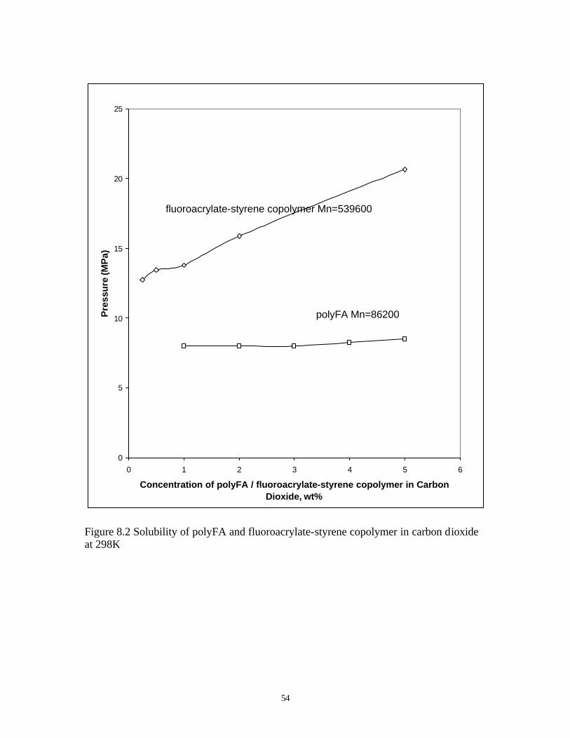
8.1 Solubility Results
8.1.1 Fluoroacrylate Homopolymer and Fluoroacrylate- styrene Copolymer
The fluoroacrylate-styrene copolymer is easily dissolved in liquid carbon dioxide, and the
mixture of copolymer and CO2 is transparent and stable. As expected, the solubility of
fluoroacrylate-styrene copolymer in CO2 does depend on the composition of the copolymer. As
shown in Figure 8.1, cloud point experiments at 297 K indicate that the solubility of the
polymers decreases with increasing styrene content in the polymer chain.
Compared to polyfluoroacrylate homopolymer, fluoroacrylate-styrene random copolymer
needs slightly higher pressure to be dissolved in carbon dioxide, as shown in Figure 8.2. The
higher molecular weight and higher styrene content of the copolymer both contribute to the
diminished solubility. The molecular weights and PDI is shown in Table 8-1. The number-,
weight- and Z-average molecular, Mn, Mw and Mz, respectively, were determined using gel
permeation chromatography [American Polymer Standards Corporation].

52
Table 8- 1 Molecular weights of fluoropolymers
Mn Mw PDI Mw/RU RU #
Fluoroacrylate-
styrene
copolymer
539600 880200 1.63 622.32 867
86200 254000 2.95 518.17 166 Polyfluoroacrylate
homopolymer 232000 557000 2.40 518.17 448
8.1.2 Styrene - FA- x Copolymer Solubility
The result of random styrene-FA-x Copolymer is not promising, both the homopolymer
and copolymer cannot dissolve in CO2 well, although both swell significantly in pure CO2 at
5000psi. The mixture of homopolymer and CO2 is kind of transparent, below the pure CO2
phase. The mixture of copolymer and CO2 is opaque even at 6000 psi. After depressurization, no
foam, no gel appeared in both cases.
Therefore the FA-x, a perfluoroalkyl ethyl acrylate, is not CO2-philic enough. This is in
agreement with previous observations that acrylates are more carbon dioxide-soluble than
methacrylates or ethacrylates.

53
1000
1500
2000
2500
3000
3500
4000
0 1 2 3 4 5 6
Concentration (wt%)
Clo
ud
po
int (
psi
)
26%styrene 29%styrene 30%styrene 35%styrene
Figure 8.1 Fluoroacrylate-styrene copolymer cloud point vs concentration (T=297K)
54
0
5
10
15
20
25
0 1 2 3 4 5 6
Concentration of polyFA / fluoroacrylate-styrene copolymer in Carbon Dioxide, wt%
Pre
ssu
re (M
Pa)
polyFA Mn=86200
fluoroacrylate-styrene copolymer Mn=539600
Figure 8.2 Solubility of polyFA and fluoroacrylate-styrene copolymer in carbon dioxide at 298K

55
8.1.3 Temperature Effect on the Fluoroacrylate- styrene Copolymer Solubility
The fluoroacrylate-styrene ransom copolymer is soluble in dense carbon dioxide at
concentration up to 5wt% at 298K, 323K, 348K and 373K, as illustrated in figure 8.3. The cloud
point curve shifted toward higher pressure with increasing concentration and temperature.
The cloud point pressure at any given temperature must be contrasted with the minimum
miscibility pressure, MMP, at the same temperature to establish the solubility of the copolymer
at reservoir conditions. For example, consider a carbon dioxide miscible project with a
minimum miscibility pressure of 18 MPa (2616 psia). Figure 8.3 indicates that at a temperature
of 298 K and a pressure of 18 MPa, roughly 3wt% of the copolymer could be dissolved in CO2;
more than enough to significantly thicken the CO2. At a reservoir temperature of 323 K and a
pressure of 18 MPa, about 0.5wt% of the copolymer could be dissolved in CO2; roughly the
lowest amount of copolymer needed to make a significant (e.g. doubling) increase in CO2
viscosity. At a pressure of 18 MPa and 348 K or 373 K, the solubility of the copolymer in CO2
would be much less than 0.25wt%; insufficient to induce an appreciable viscosity change.
If greater copolymer solubility is required at the reservoir conditions than is possible with
the 79%fluoroacrylate-21%styrene copolymer with a number average molecular weight of
540,000, then a copolymer of comparable molecular weight with a slightly greater fluoroacrylate
composition and/or a lower molecular weight would be required[4.29] , thereby making the
copolymer more CO2 soluble. This modification would reduce the thickening capability of the
copolymer, however, and a slightly greater concentration of the copolymer would be required to
attain a desired level of viscosity.

56
10
15
20
25
30
35
40
45
0 1 2 3 4 5 6
Concentration of Copolymer in Carbon Dioxide, wt%
Pre
ssu
re (
MP
a)
298K
323K
348K
373K
Figure 8.3 Effect of Temperature on the solubility of the fluoroacrylate- styrene copolymer in
carbon dioxide
57
8.2 Falling Cylinder Viscometer Results
8.2.1 Aldrich Fluoroacrylate- styrene Copolymer
From falling cylinder viscometer, all these copolymer can increase CO2 viscosity by
several orders at relatively low concentration. After we found the best relative viscosity increase
of 29mol%Styrene-71mol%FluoroAcrylate copolymer, we tested it extensively, with different
falling cylinders and different copolymer concentrations. For our best fluoroacrylate-styrene
copolymer (29mol% styrene), the relative viscosity of CO2 solution (ηη
so
CO
ln.2
) is much enhanced,
from 2 to 200 times, relative to concentration from 0.2wt% to 5wt%. Because the viscosity is
strongly related to shear rate, so, we examined the relative viscosity with different falling
cylinder size, see the Figure 8.4.
From the figure, we can see, the viscosity of CO2 is enhanced more than 200 times in
5wt% copolymer-CO2 solution, and even in 1wt% solution, the viscosity of CO2 was increased
several times. In lower concentration, 0.2wt% or 0.1wt%, there is still discernible viscosity
increase at high shear rates. This viscometer is not suited for the determination of the relative
viscosity at the low shear rates associated with creeping flow through porous media (10s-1).
Further, the results (based on a Newtonian fluid assumption) illustrated in Figure 8.4 clearly
indicate that the fluid is not Newtonian. Therefore, a power law model description of the fluid
was derived.
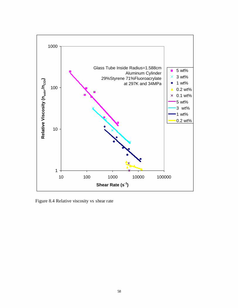
58
1
10
100
1000
10 100 1000 10000 100000
Shear Rate (s-1)
Rel
ativ
e V
isco
sity
(nso
ln./n
CO
2)
5 wt%3 wt%1 wt%0.2 wt%0.1 wt%5 wt%3 wt%1 wt%0.2 wt%
Glass Tube Inside Radius=1.588cmAluminum Cylinder
29%Styrene 71%Fluoroacrylateat 297K and 34MPa
Figure 8.4 Relative viscosity vs shear rate
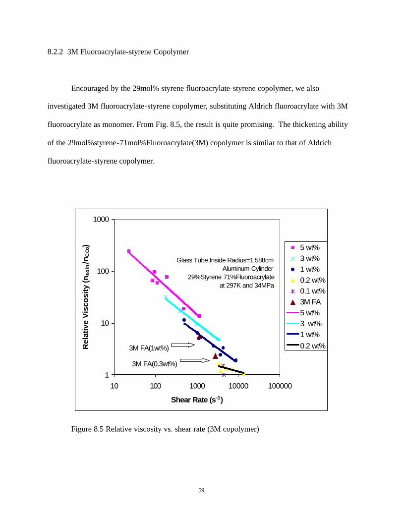
59
8.2.2 3M Fluoroacrylate- styrene Copolymer
Encouraged by the 29mol% styrene fluoroacrylate-styrene copolymer, we also
investigated 3M fluoroacrylate-styrene copolymer, substituting Aldrich fluoroacrylate with 3M
fluoroacrylate as monomer. From Fig. 8.5, the result is quite promising. The thickening ability
of the 29mol%styrene-71mol%Fluoroacrylate(3M) copolymer is similar to that of Aldrich
fluoroacrylate-styrene copolymer.
1
10
100
1000
10 100 1000 10000 100000
Shear Rate (s-1)
Rel
ativ
e V
isco
sity
(nso
ln./n
CO
2) 5 wt%3 wt%1 wt%0.2 wt%0.1 wt%3M FA5 wt%3 wt%1 wt%0.2 wt%
Glass Tube Inside Radius=1.588cmAluminum Cylinder
29%Styrene 71%Fluoroacrylateat 297K and 34MPa
3M FA(1wt%)
3M FA(0.3wt%)
Figure 8.5 Relative viscosity vs. shear rate (3M copolymer)

60
8.2.3 Temperature Effect on the Fluoroacrylate- styrene Copolymer Thickening Ability
Figures 8.4 and 8.5 indicate that the 29% styrene fluoroacrylate-styrene copolymer has
good thickening capacity at ambient temperature, 297 K. Reservoir temperatures extend to 393
K, however. Literature[43] indicated that there may be a temperature effect on the properties of
the atoms in the regions of intermolecular contact via stacking of the phenyl groups. The change
in temperature may influence the strength and geometry of interactions, which may result in the
change of local molecular environment. This may affect the π-π stacking capacity and
thickening capability of the fluoroacrylate-styrene copolymer. Because the majority of CO2
flooding projects are conducted in reservoirs at temperatures between 25~100°C, we tested the
fluoroacrylate-styrene copolymer thickening ability over this temperature range. The
fluoroacrylate-styrene copolymer thickening capacity was determined using the 1.2428”
diameter fa lling aluminum cylinder at temperatures of 25°C, 50°C, 75°C and 100°C. Table 8-2
indicates that the temperature doesn’t have significant effect on the π-π stacking phenomena.
Table 8-2 Temperature effect on the solution relative viscosity
The fluoroacrylate-styrene copolymer concentration Temperature (°C)
1 wt% 0.3 wt%
25 2.3 1.5
50 2.3 1.5
75 2.1 1.5
100 1.9 1.4

61
8.2.4 Non- Newtonian Fluid
With the assumption of the polymer/CO2 solution fit the power- law model (Appendix B),
we can get the power law model constants from the experimental falling cylinder terminal
velocity, with the minimum difference between calculated velocity and experimental velocity,
which is shown in Table 8-3.
Table 8- 3 Experimental falling cylinder terminal velocity Unit: cm.s-1
Rc 5wt% 3wt% 1wt% 0.2wt% 0.1wt%
1.245 0.04997 0.06
1.2438 0.0023
0.004104
0.00479 0.03022
0.01325
0.093
1.2428 0.00388 0.01356 0.03597 0.174 0.15
1.2399 0.02536
0.004945
0.05091 0.1957
0.1334
0.362
1.2339 0.015 0.35 1.08
1.2311 0.118 0.33 0.84
According to Appendix B (equation 18), a computer program was used to determine the
values of m and n that provided the best fit of the viscosity data at each temperature. The
computer program is attached in Appendix C. The results are provided in Table 8-4 and Figures
8.6 and 8.7
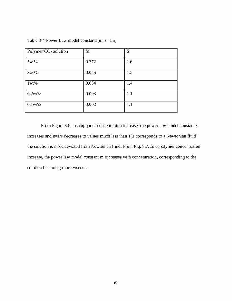
62
Table 8-4 Power Law model constants(m, s=1/n)
Polymer/CO2 solution M S
5wt% 0.272 1.6
3wt% 0.026 1.2
1wt% 0.034 1.4
0.2wt% 0.003 1.1
0.1wt% 0.002 1.1
From Figure 8.6 , as coplymer concentration increase, the power law model constant s
increases and n=1/s decreases to values much less than 1(1 corresponds to a Newtonian fluid),
the solution is more deviated from Newtonian fluid. From Fig. 8.7, as copolymer concentration
increase, the power law model constant m increases with concentration, corresponding to the
solution becoming more viscous.

63
0
0.2
0.4
0.6
0.8
1
1.2
1.4
1.6
1.8
0 1 2 3 4 5 6
copolymer solution wt%
con
stan
t s, n
s
n
Figure 8.6 power law constant s, n(=1/s) (T=297K, P=34MPa)

64
0.001
0.01
0.1
1
0 1 2 3 4 5 6
copolymer solution wt%
con
stan
t m
Figure 8.7 power law constant m (T=297K, P=34MPa)

65
Using the power model found in Appendix B, these results were illustrated in Fig 8.8.
These results also indicate that the fluoroacrylate-styrene copolymer is an effective carbon
dioxide thickener.
8.3 Flow- through- porous - media Viscometer Results
In order to simulate the field CO2 flooding, we did experiment at superficial velocities of
both 1 ft/day and 10ft/day flow rate. The permeability of the Berea sandstone cores was 80-200
md, as determined from experiments using neat carbon dioxide. The pressure drop was, as
expected, much higher in 10 ft/day displacements. At the same flow rate, significantly higher
pressure drops were detected for the fluoroacrylate-styrene copolymer/carbon dioxide solutions
than for neat carbon dioxide.
The pressure drops along the core were on the order of 100-100000 Pa, depending on the
superficial velocity and the copolymer concentration. This pressure drop was small relative to the
pressure at the inlet face of the sandstone, which was maintained at 20MPa.
The pressure drops along each third of the core varied by no more than 5% for every
mobility measurement. The variations were random, with no section of the core (particularly the
inlet section) exhibiting a consistently greater pressure drop than the other sections. Therefore,
no evidence of copolymer retention at the inlet face of the core was detected.

66
0.1
1
10
100
10 100 1000 10000 100000
Shear Rate (s-1)
Rel
ativ
e V
isco
sity
(n
/u C
O2)
5 wt%
3 wt%
1 wt%
0.2 wt%
0.1 wt%
5 wt%
3 wt%
1 wt%
0.2 wt%
Glass Tube Inside Radius=1.588cm
Aluminum Cylinder29%Styrene 71%Fluoroacrylate
at 297K and 34MPa
Figure 8.8 Relative Viscosity vs Shear Rate (Power Law)
67
Pressure drops of the neat and thickened carbon dioxide, flowing at the same superficial
velocity, were used to estimate the increase in carbon dioxide viscosity. This viscosity increase at
298K and 20MPa is presented as a function of copolymer concentration for a constant superficial
velocity, as illustrated in Table 8-5 and Figure 8.9. The pressure drops for both 1ft/day and
10ft/day are illustrated in Figure 8.10 and Figure 8.11.
The minimum concentration of thickener required to realize a significant increase in
viscosity is about 0.5 wt%, while copolymer concentration as low as 0.25wt% were capable of
thickening carbon dioxide. Significant increases in viscosity are attained as the concentration of
the thickener increases to several weight percent. The 1.0wt% and 1.5wt% copolymer solution
were 8 and 19 times more viscous than neat carbon dioxide, respectively, at a velocity of
0.00035cm/s (1 ft/day).
Because of the shear-thinning nature of the copolymer, increases in superficial velocity
led to diminished thickening capability. For example, the addition of 1.5wt% copolymer
increased the carbon dioxide viscosity by a factor of only 2 at a superficial velocity of 0.028cm/s
(80 ft/day).
The permeability of the core to neat carbon dioxide that was injected after the copolymer
solution agreed with the original measurement of permeability to within 1wt%. Therefore, the
flow of the copolymer solution through the sandstone core did not result in any detectable
permeability reduction.
These are the first measurements of a thickened carbon dioxide solution that requires no
cosolvent and that elevates the viscosity of carbon dioxide by an order of magnitude at a
concentration of only 1 wt%. This demonstrates that a carbon dioxide thickener can be
developed if one designs the thickener specifically for dissolution in CO2.

68
Table 8-5 Berea core flooding results
∆Psolution/∆PCO2 Flow rate
0wt% 0.2wt% 0.5wt% 1wt% 1.5wt% 2wt%
1 1.1 1.33 3.05 5.3 10.0
1 1.05 1.38 2.96 5.1 11.0
1 1.02 1.45 3.63 6.0 9.8
1ft/day
1 1.04 1.61 3.61
1 1.04 1.29 3.20 5.0 8.9
1 1 1.27 2.82 5.0 8.8
1 2.69 4.9 8.3
10ft/day
1 2.82

69
0
2
4
6
8
10
12
14
16
18
20
0 0.5 1 1.5 2
Concentration of Copolymer in Carbon Dioxide, wt%
Rel
ativ
e V
isco
sity
Incr
ease
0.00035cm/s
0.0035cm/s
0.018cm/s
0.028cm/s
Figure 8.9 Relative viscosity increase vs. concentration at 298K, 20MPa, flowing through
~100md Berea sandstone
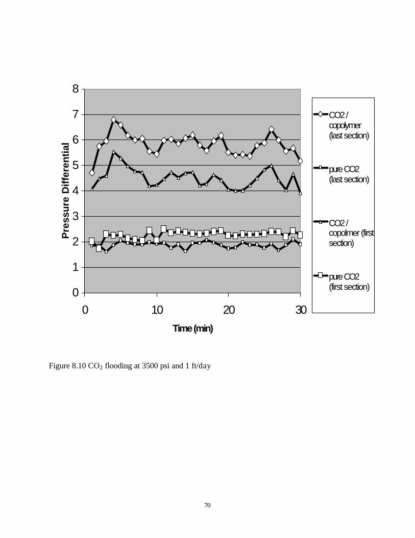
70
0
1
2
3
4
5
6
7
8
0 10 20 30Time (min)
Pre
ssu
re D
iffe
ren
tial
CO2 /copolymer(last section)
pure CO2(last section)
CO2 /copolmer (firstsection)
pure CO2(first section)
Figure 8.10 CO2 flooding at 3500 psi and 1 ft/day

71
0
10
20
30
40
50
60
0 10 20 30Time (min)
Pre
ssu
re D
iffe
ren
tial
CO2 /copolymer(lastsection)pure CO2(lastsection)
CO2 /copolymer(firstsection)pure CO2(firstsection)
Figure 8.11 CO2 flooding at 3500 psi and 10 ft/day
72
9.0 NON-FLUOROUS POLYMERS RESULTS
The fluoroacrylate-styrene copolymer is a direct thickener in that it does not require a
cosolvent. Nonetheless, the fluoroacrylate-styrene copolymer is a highly fluorinated copolymer
that is expensive, unavailable in large quantities and environmentally persistent. Rather than
continuing to enhance the properties of fluoroacrylate-styrene copolymer (e.g. adjusting the
composition and molecular weight (Mn) to attain higher solubility of fluoroacrylate-styrene
copolymer at a specified pressure), a new generation of CO2 thickeners has been designing at the
University of Pittsburgh. Specifically, our current studies have been keeping focusing on
inexpensive, biodegradable, non-fluorous direct thickeners that can be produced in large amounts
and do not require an organic cosolvent to achieve dissolution. The same strategy used in the
development of fluoroacrylate-styrene copolymer is being employed in the development of the
non-fluorous thickener. Novel copolymers composed of carbon, hydrogen, oxygen and nitrogen
has been designed to exhibit high CO2 solubility. CO2-phobic, associating groups will then be
incorporated into the copolymer to impart thickening capabilities. The associating group content
of the thickener composition will be adjusted to attain a reasonable balance of CO2 solubility and
thickening capability.
Non-fluorous thickening agents have not been identified yet. Work to date has being
concentrated only on the identification of highly carbon dioxide-soluble, non-fluorous polymers.
If such a polymer can be identified, it will then be modified to enhance its thickening capability.
Some preliminary solubility results for the hydrocarbon-based polymers are presented below.
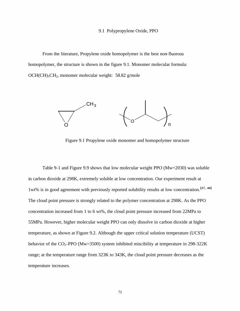
73
9.1 Polypropylene Oxide, PPO
From the literature, Propylene oxide homopolymer is the best non-fluorous
homopolymer, the structure is shown in the figure 9.1. Monomer molecular formula:
OCH(CH)3CH2, monomer molecular weight: 58.82 g/mole
O
CH3
O n
Figure 9.1 Propylene oxide monomer and homopolymer structure
Table 9-1 and Figure 9.9 shows that low molecular weight PPO (Mw=2030) was soluble
in carbon dioxide at 298K, extremely soluble at low concentration. Our experiment result at
1wt% is in good agreement with previously reported solubility results at low concentration.[27, 44]
The cloud point pressure is strongly related to the polymer concentration at 298K. As the PPO
concentration increased from 1 to 6 wt%, the cloud point pressure increased from 22MPa to
55MPa. However, higher molecular weight PPO can only dissolve in carbon dioxide at higher
temperature, as shown at Figure 9.2. Although the upper critical solution temperature (UCST)
behavior of the CO2-PPO (Mw=3500) system inhibited miscibility at temperature in 298-322K
range; at the temperature range from 323K to 343K, the cloud point pressure decreases as the
temperature increases.

74
90
100
110
120
130
140
320 325 330 335 340 345
LIQUID + LIQUID
FLUID
Pres
sure
(MPa
)
Temperature (K)
CH2 CHO n
CH3
Figure 9.2 Cloud - point curve for ~5 wt% poly(propylene oxide) (PPO, M w = 3500) – CO2
mixture. Data from lab of Dr. Mark McHugh provided by Zhihao Shen of Virginia
Commonwealth University.
9.2 Polybutadiene
The polybutadiene series polymers, including original polybutadiene from Aldrich
(Mn=1200), polybutadiene with hydroxyl end and polybutadiene with acetate end, were not
completely soluble in CO2 at 7000psia and 1wt% concentration. The structure of the butadiene
monomer and homopolymer, and acetate end-capped polybutadiene is shown in figure 9.3.
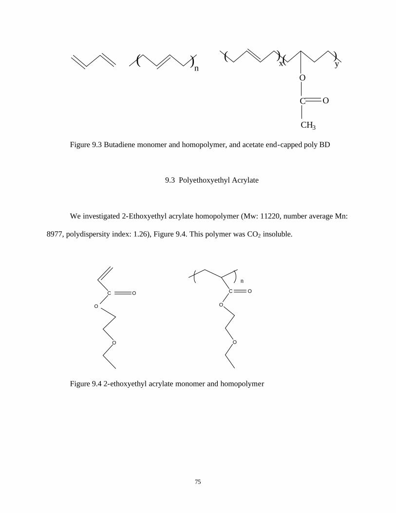
75
)(n
O
C
CH 3
O
() )(x y
Figure 9.3 Butadiene monomer and homopolymer, and acetate end-capped poly BD
9.3 Polyethoxyethyl Acrylate
We investigated 2-Ethoxyethyl acrylate homopolymer (Mw: 11220, number average Mn:
8977, polydispersity index: 1.26), Figure 9.4. This polymer was CO2 insoluble.
C O
O
O
C O
O
O
n
Figure 9.4 2-ethoxyethyl acrylate monomer and homopolymer
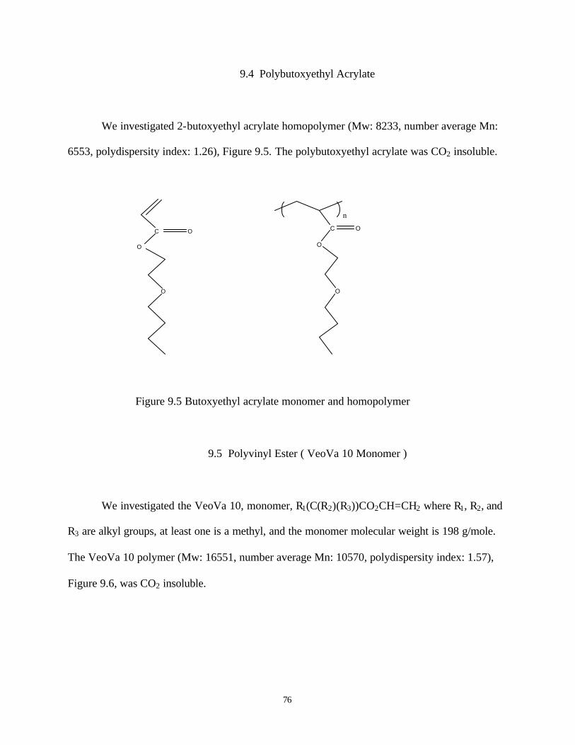
76
9.4 Polybutoxyethyl Acrylate
We investigated 2-butoxyethyl acrylate homopolymer (Mw: 8233, number average Mn:
6553, polydispersity index: 1.26), Figure 9.5. The polybutoxyethyl acrylate was CO2 insoluble.
C O
O
O
C O
O
O
n
Figure 9.5 Butoxyethyl acrylate monomer and homopolymer
9.5 Polyvinyl Ester ( VeoVa 10 Monomer )
We investigated the VeoVa 10, monomer, R1(C(R2)(R3))CO2CH=CH2 where R1, R2, and
R3 are alkyl groups, at least one is a methyl, and the monomer molecular weight is 198 g/mole.
The VeoVa 10 polymer (Mw: 16551, number average Mn: 10570, polydispersity index: 1.57),
Figure 9.6, was CO2 insoluble.

77
O
C O
R1
R2R3
HC O
R 3
R 1
R 2
O
n
Figure 9.6 VeoVa 10 monomer and homopolymer
9.6 Poly Vinyl Acetate, PVAc
PVAc is the vinyl acetate homopolymer, the structure is shown in Figure 9.7. We
synthesized several low molecular weight samples of PVAc and purchased from Aldrich. The
GPC results are shown in Table 9-1.
O
C O
O
C O
n
Figure 9.7 Vinyl acetate monomer and homopolymer structure
The very low PVAc solubility data proved to be comparable to that of polypropylene
oxide, although the PVAc-CO2 Px profiles were much flatter than the PPO-CO2 profiles. We

78
synthesized poly vinyl acetate using atom transfer radical polymerization in order to control
molecular weight. The extremely high cloud point pressures for some PVAc were obtained with
the help of Dr. Mark McHugh and Dr. Zhihao Shen of Virginia Commonwealth University. The
solubility results are shown in Figure 9.8 and Figure 9.9.
The CO2 solubility of polyvinyl acetate is quite promising. Polyvinyl acetate does
dissolve in CO2 in large amounts. The solubility curves for PVAc were fairly flat over a wide
range of concentration, for all the different MW samples we investigated. We also found that as
molecular weight increase, the pressure required to dissolve PVAc in carbon dioxide increase,
which is shown as expected. The results, figure 9.9, shows that the cloud point pressure, for the
two lowest molecular weight PVAc (PVA2063 and PVAc3092), are very close, almost identical,
because the lower Mn one has higher dispersity index PDI 2.01, much higher than that of the
higher Mn PVAc, which is 1.5. The broader distribution of polymers causes the high apparent
cloud point pressure.
PVAc and PPO of comparable repeat units have similar solubility at 3wt%. Above 3wt%,
PVAc is more soluble than PPO, while below 3wt%, PPO is more soluble. Unlike PVAc, PPO is
very sensitive to the sample concentration in carbon dioxide. As concentration increases, the
pressure needed to dissolve PPO in carbon dioxide increases dramatically. And at the
concentration of 6wt%, PPO solubility test is above the range of our Ronbinson Cell capacity.
However, PVAc was not as CO2-soluble as polyfluoroacrylate or the fluoroacrylate-
styrene copolymer thickener, as shown in Figure 8-2. These fluoropolymers were soluble in
carbon dioxide at much lower pressures than that of PMA, PPO and PVAc. For example, the
fluoroacrylate-styrene copolymer (Mn=539600), with 867 repeat units, is more soluble than
PVAc (Mn=3092), with 36 repeat units.

79
Figure 9.9 shows that compared with the phase behavior of molecular weight 2300 PPO,
two phase locus of PVAc-CO2 mixtures exhibits a relatively flat profile over the 1~12 wt%
region at 298K with the cloud point pressure maximum occurring near 5wt% concentration. The
cloud point pressure increases with PVAc chain length.
For even longer PVAc, the highest molecular weight PVAc (Mw=500000) in our
experiment, is still soluble in carbon dioxide at 298K at a pressure of 68MPa. The temperature –
cloud point pressure relationship is illustrated in figure 9.8, for two high molecular weight PVAc
samples (Mw=125000 and Mw=585000). The strength of the CO2-acetate interaction is
apparently great enough to overcome repeat group-repeat group interactions, and entropic effects
associated with polymer conformation do not have a dramatic effect on the cloud point pressure.
From Figure 9.8 and Figure 9.9, higher molecular weight PVAc need higher pressure to get
dissolved in carbon dioxide.
In Figure 9.9, we also compared the cloud point pressure of poly propylene oxide (PPO),
poly vinyl acetate (PVAc), and poly methyl acetate (PMA), the molecular weight is also listed in
the figure 9.9. More physical property information is available in Table 9.1.
Although PVAc is a promising non-fluorous, carbon dioxide soluble homopolymer, it is
far less CO2-philic than fluoroalkyl acrylate polymers (PFA). PFA typically has a linear side-
chain terminated with a long fluorocarbon segment, such as poly(heptadecafluorodecyl acrylate).
DeSimore pioneered the incorporation of fluoroalkyl acrylate into a homopolymer or
copolymer to attain carbon dioxide solubility.[45] Figure 9.12 illustrates that the cloud point
pressure of PFA are significantly lower than those of PVAc.[46-48] This difference is contributed
to CO2-phobic attribute of PVAc relative to PFA at low pressures, which has been used to
facilitate the emulsion polymerization of vinyl acetate in carbon dioxide.[49]

80
Despite having identified PVAc as the most CO2 soluble, non-fluorous, commercial
polymer, the pressure required to dissolve high molecular weight PVAc is much greater than the
MMP of CO2 floods. Therefore, PVAc is not CO2-philic enough to serve as the polymeric basis
of non-fluorous CO2 thickeners.
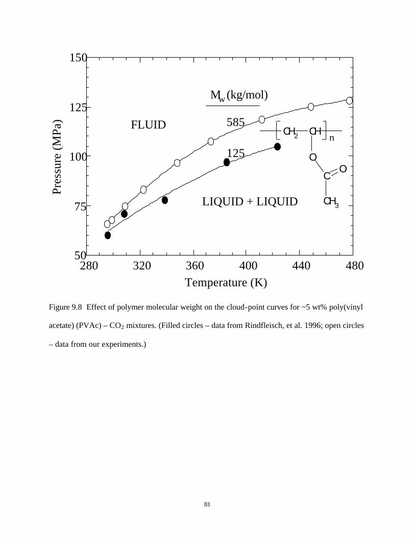
81
50
75
100
125
150
280 320 360 400 440 480
LIQUID + LIQUID
FLUID
Mw (kg/mol)
585
Pres
sure
(MPa
)
Temperature (K)
125 O
CH3
CH2 CHn
CO
Figure 9.8 Effect of polymer molecular weight on the cloud - point curves for ~5 wt% poly(vinyl
acetate) (PVAc) – CO2 mixtures. (Filled circles – data from Rindfleisch, et al. 1996; open circles
– data from our experiments.)

82
20
30
40
50
60
70
80
90
100
0 5 10 15 20
Concentration in CO2 (wt%)
Pre
ssu
re (
MP
a)
PVA (Mn=2063, PDI=2.01)
PVA (Mn=3092, PDI=1.5)
PVA (Mn=7697, PDI=1.62)
PVA (Mn=12991, PDI=1.31)
PMA (Mn=2079, PDI=1.37)
PPO (Mn=2000)
PMA (Mn=2321, PDI=1.45)
PVA (Mn=52700, PDI =2.37)
Figure 9.9 Phase behavior of PVA, PPO and PMA at 298K

83
9.7 Poly Methyl Acrylate, PMA
PMA is identical to PVAc except that the position of the carbonyl is switched. To make a
valid comparison, short polymers or oligimers of PPO, PVAc and PMA were employed.
Samples of PMA and PVAc with comparable molecular weight or number of repeat units
relative to PPO 2000 were prepared. Monomer molecular formula: H2C=CHCO2CH3, monomer
molecular weight: 86.09, compound structure is shown in Figure 9.10.
O
O
O
O
( ) n
Figure 9.10 Methyl acrylate monomer and homopolymer
To make the comparison more meaningful, we compared PPO, PVAc and PMA with the
same number of repeat unit or same molecular weight, corresponding to PPO 2000. With the
small difference in the structure between PMA and PVAc, a big solubility difference was
exhibited. We cannot dissolve the PMA in our Ronbinson Cell, Dr. Mark McHugh at Virginia
Commonwealth University helped us get the extremely high cloud point pressures. The pressure
required to dissolve the higher molecular weight PMA (Mn=2321) is slightly less than that
required for the lower molecular weight sample (Mn=2079). We attribute this unusual trend to
84
residual amounts of co-solvent that were left in the PMA 2321 sample, because the PMA 2321
was less viscous than, not more viscous as it was supposed to, the PMA 2079. The solubility
results are shown in Figure 9-10.
From the solubility data of PMA and PMAc, it is quite interesting to know why a little
change in the structure causes such a big solubility difference. It is expected the relative position
of carboynal group and backbone carbon chains play an important role here, as well as the ether
oxygen. The real atom and molecular correlation, and pros and cons for the carbon dioxide
solubility are still under investigation, with the help of Dr. Johnson of Chemical and Petroleum
Engineering Department at the University of Pittsburgh.
With the help from Dr. Mark McHugh at Virginia Commonwealth University, we also
investigated the temperature effect on the PMA carbon dioxide solubility. From Figure 9-11, at
temperature range between 25-50°C, at low concentration, as the PMA concentration increase,
the required pressure to dissolve PMA also increases; while at higher concentration (>5wt%), the
concentration doesn’t have a big effect on the required pressure. The PMA isotherms exhibit a
maximum value at about 5wt% PMA at each temperature, which has been previously observed
by other polymer-solvent mixtures. [25, 50-54]
PMA is much less soluble in carbon dioxide than PVAc even though the repeat group of
both polymers is slightly rearranged. Figure 9.12 illustrates that the cloud point pressure of PMA
increases dramatically as the molecular weight increases, while cloud point pressure of PVAc
increases much slower than that of PMA. Because PMA carbonyl group is closer to the polymer
backbone, which can not move freely; on the other hand, the PVAc carbonyl group can rotate
freely due to the ether linkage between the polymer backbone and the acetate.

85
60
70
80
90
100
110
0 2 4 6 8 10 12Poly(methyl acrylate) Concentration (wt%)
Pres
sure
(MPa
)FLUID
LIQUID + LIQUID
T (K)
298
313
323
CH2 CH n
C
O
CH3
O
Figure 9.11 Pressure-composition isotherms for the system CO2 – poly(methyl acrylate) (PMA)
(Mw = 2850) at 298, 313, and 323 K. High pressure data ( >70MPa) provided by Mark McHugh
and Zhihao Shen of Virginia Commonwealth University.
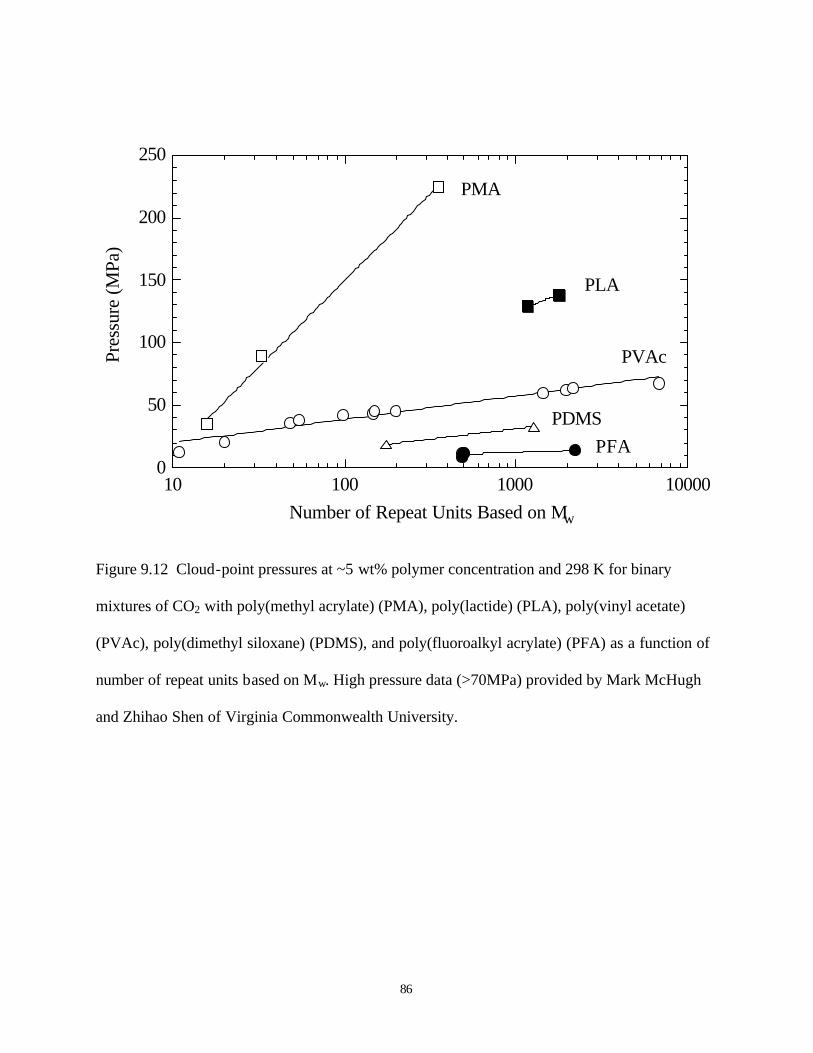
86
0
50
100
150
200
250
10 100 1000 10000
Pres
sure
(MPa
)
Number of Repeat Units Based on Mw
PLA
PVAc
PDMSPFA
PMA
Figure 9.12 Cloud - point pressures at ~5 wt% polymer concentration and 298 K for binary
mixtures of CO2 with poly(methyl acrylate) (PMA), poly(lactide) (PLA), poly(vinyl acetate)
(PVAc), poly(dimethyl siloxane) (PDMS), and poly(fluoroalkyl acrylate) (PFA) as a function of
number of repeat units based on Mw. High pressure data (>70MPa) provided by Mark McHugh
and Zhihao Shen of Virginia Commonwealth University.

87
9.8 Poly Vinyl Formate, PVF
Encouraged by the promising result of PVAc, we investigated poly vinyl formate (Mw:
2327, number average Mn: 1068, polydispersity index: 2.18), Figure 9.13, which is identical in
structure to poly vinyl acetate except that the methyl of the acetate is replaced by hydrogen.
Recently, Scott Wallen and coworkers have indicated that a cooperative weak hydrogen bond
may occur between the oxygen of CO2 and the terminal hydrogen of the formate monomer. This
interaction may lead to enhanced carbon dioxide solubility of poly vinyl formate.[55]
O
HC O
O
HC O
n
Figure 9.13 Vinyl formate monomer and homopolymer
Poly vinyl formate is cannot dissolve in carbon dioxide. This result is consist with the
previous observations,[25, 56] which concluded that very polar or hydrogen bonded polymers do
not dissolve in carbon dioxide. Vinyl formate will interact with itself more strongly than that of
acetate, even though the formate proton is not highly acidic. Nonetheless, this interaction with
itself is much stronger than the CO2-formate interaction, causing PVF to be carbon dioxide
insoluble.

88
9.9 Methyl Isobutyrate (MIB) and Isopropyl Acetate (IPA)
The carbon dioxide solubility difference between methyl acrylate and vinyl acetate is so
significant, with a little difference in their structure. We decided to study methyl isobutyrate and
isopropyl acetate. These compounds serve as models of the repeat unit of PMA and PVAc,
respectively. They both have the same molecule composition, have molecular formulas:
(CH3)2CHCO2CH3 and CH3CO2CH(CH3)2, respectively. We tried to investigate the effect of the
structure difference on small molecular. The structures of the MIB and IPA are shown in Figure
9.14.
C
O
OCH3C
CH O C
O
CH3
Figure 9.14 methyl isobutyrate and isopropyl acetate
MIB and IPA have the same molecular formula, with the small dislocation of the atoms
in the structure. They have the similar carbon dioxide solubility. The solubility results of MIB
and IPA are shown in Figure 9.15. So, the solubility results from MIB and IPA proved that the
structure dislocation doesn’t have effect on small molecules. From Figure 9.12, the dislocation of
the carbonyl group with the molecules has no effect in solubility in small molecules, while there
is a significant effect on the solubility in polymers.
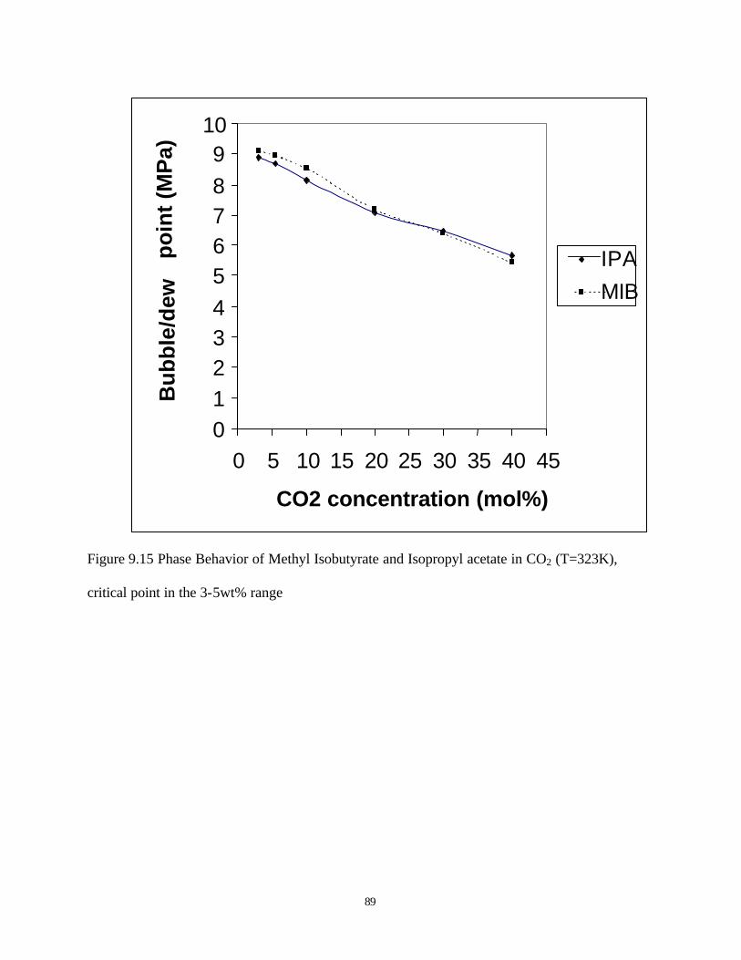
89
Figure 9.15 Phase Behavior of Methyl Isobutyrate and Isopropyl acetate in CO2 (T=323K),
critical point in the 3-5wt% range
0
1
2
3
4
5
6
7
8
9
10
0 5 10 15 20 25 30 35 40 45
CO2 concentration (mol%)
Bu
bb
le/d
ew
po
int
(MP
a)
IPA
MIB

90
9.10 Poly Dimethyl Siloxane
The solubpoly dimethyl siloxane in carbon dioxide has been previous reported at
298K.[27, 57] Silicone homopolymers are also more carbon dioxide soluble than PVAc as seen in
Figure 9.12, although PDMS is not as carbon dioxide soluble as PFA. The structure of PDMS is
shown in Figure 9.16.
Si O( )n
Figure 9.16 Poly (dimethyl siloxane) structure

91
Table 9-1 Molecular weight of PMA, PVAc, PPO and PVF*.
Polymer Mn Mw Mw/Mn NRU,n NRU,w Pcp (MPa)
780 1390 1.78 9 16 34.6 2080 2850 1.37 24 33 89.1
PMA
10600 30700 2.90 123 357 225.0 a
780 980 1.25 9 11 13.6 850 1700 2.00 10 20 20.8
2060 4150 2.01 24 48 37.4 3090 4640 1.5 36 54 37.6 5680 8380 1.47 66 97 42.0 7700 12500 1.62 89 145 43.6
12800 149 45.7 13000 17000 1.31 151 198 45.7 52700 124800 2.37 612 1451 60.2 a
167000 1941 62.5 61600 182000 2.95 716 2116 63.7
PVAc
193000 585000 3.02 2244 6802 67.6
1640 2030 1.24 28 35 43.6 PPO
3500 60 Insoluble
PVF 1070 2327 2.18 15 27 Insoluble
a Data from Rindfleisch, et al. 1996. * This table includes number averaged molecular weight (Mn), weight averaged molecular
weight (Mw), polydispersity (Mw/Mn), number of repeat units based on Mn (NRU,n), and number
of repeat units based on Mw (NRU,w), for poly(methyl acrylate) (PMA), poly(vinyl acetate)
(PVAc), poly(propylene oxide) (PPO), and poly(vinyl formate) (PVF) and cloud-point pressures
(Pcp) for their binary mixtures with CO2 at ~5 wt% and 298 K.
92
10. 0 CONCLUSION AND FUTUR E WORK
1. We have successfully identified the first CO2 thickener, the fluoroacrylate-styrene
random copolymer (71mol% fluoroacrylate-29mol% styrene) synthesized via bulk, free-
radical polymerization. This copolymer has a number-average molecular weight of
540,000 and a polydispersity index of 1.63. The fluoroacrylate-styrene copolymer
exhibited remarkably high solubility in dense carbon dioxide, which was attributed to the
high fluoroacrylate content of the copolymer.
2. The thickening capability of fluoroacrylate-styrene copolymer over the 298 – 373 K
temperature range was attributed to intermolecular p-p stacking of the aromatic rings
associated with the styrene monomer. Previous research demonstrated that fluoroacrylate
copolymers lacking the pendent phenyl group did not thicken CO2.
3. Pressure drop measurements of the fluoroacrylate-styrene copolymer-carbon dioxide
solutions flowing through Berea sandstone demonstrated that the fluoroacrylate-styrene
copolymer could effectively reduce the mobility of carbon dioxide at superficial
velocities up to 0.0035cm/s (10ft/day). Higher velocities and lower copolymer
concentration resulted in much smaller reductions in mobility. For example, the apparent
viscosity of carbon dioxide was increased by a factor of 7-8 at superficial velocities of
0.00035-0.0035cm/s (1-10ft/day) for a 1wt% solution of the copolymer in carbon
dioxide, and the apparent viscosity of carbon dioxide was increased by a factor of 12-19
at the same velocities range for 1.5wt% solution.
4. The fluoroacrylate-styrene copolymer-carbon dioxide solution illustrated shear-thinning
behavior. As the shear rate increases, the viscosity of the solution decreases.

93
5. Poly vinyl acetate is the most promising non-fluorous base polymer, composed of carbon,
hydrogen and oxygen, identified up to date. The high solubility is reflected by the
relatively low pressure required to attain dissolution of approximately 5wt% polymer at
298K. Unfortunately, the pressure required to dissolve PVAc in CO2 greatly exceed the
MMP of CO2 floods. Therefore, PVAc is not CO2-philic enough to be used in the design
of CO2 thickeners.
6. Other carbonyl-rich polymers, including PMA, containing similar functional groups were
significantly less soluble or insoluble in carbon dioxide due to their crystallinity, lack of
side chains, or less accessible to carbonyl groups.
7. Less expensive CO2-philic functional groups are to be developed to replace the more
expensive fluorous CO2-philic functionalities in the thickener structures. Ideally,
hydrocarbon based structures, which is bio-degradable, are to be incorporated into the
CO2 thickener structures, to make it environmentally benign, as well as economically
possible.
8. We will continue designing our non-fluorous base polymers, and find a better base
polymer more CO2 soluble than PVAc, hopefully the new hydrocarbon-based non-
fluorous base polymer can match the solubility of the fluoroacrylate-base polymers. After
that, we will incorporate CO2-phobic, interacting groups into the polymer in order to
greatly increase the CO2 solution viscosity.

APPENDICES
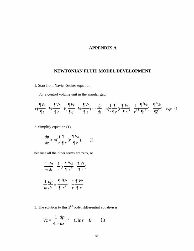
95
APPENDIX A
NEWTONIAN FLUID MODEL DEVELOPMENT
1. Start from Navier-Stokes equation:
For a control volume unit in the annular gap,
( )ρ∂
∂
∂
∂
∂
∂ θ
∂
∂µ
∂∂
∂∂
∂
∂θ
∂
∂ρθ( ) ( ( ) ( ) )
Vz
tVr
Vz
rV
VzVz
Vz
zdpdz r r
rVzr r
Vz Vz
Zgz+ + + = − + + + +
1 112
2
2
2
2
2. Simplify equation (1),
( )dpdz r r
rVz
r= µ
∂
∂
∂
∂( ( )1
2
because all the other terms are zero, so
1 1 2
2µ∂∂
∂∂
dpdz r
rVzr
Vzr
= +( )
1 12
2µ
∂
∂
∂
∂dpdz
Vz
r r
Vz
r= +
3. The solution to this 2nd order differential equation is:
( )Vzdpdz
r C r B= + +1
432
µln
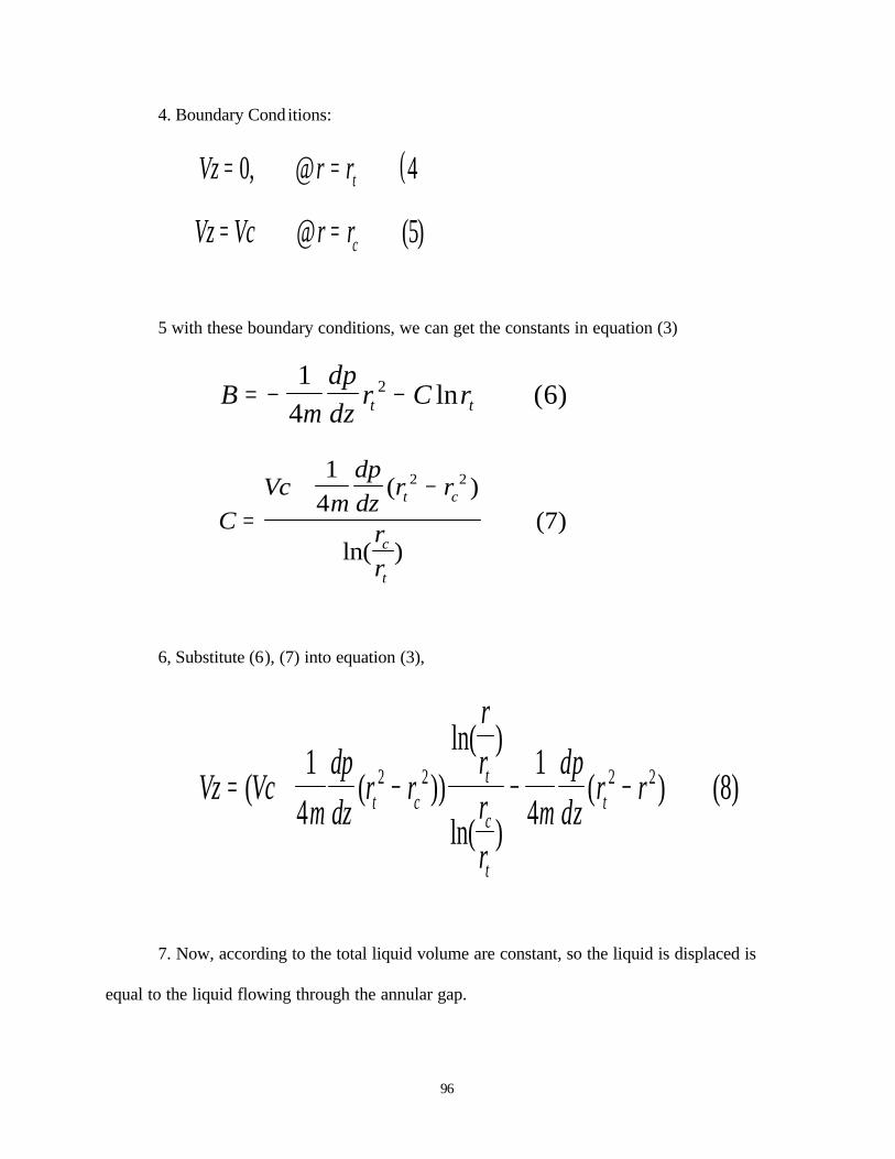
96
4. Boundary Cond itions:
( )Vz r rt= =0 4, @
Vz Vc r rc= =@ (5)
5 with these boundary conditions, we can get the constants in equation (3)
B
dpdz
r C rt t= − −1
462
µln ( )
C
Vcdpdz
r r
rr
t c
c
t
=+ −
14
7
2 2
µ( )
ln( )( )
6, Substitute (6), (7) into equation (3),
Vz Vcdpdz
r r
rrrr
dpdz
r rt ct
c
t
t= + − − −( ( ))ln( )
ln( )( ) (8)
14
14
2 2 2 2
µ µ
7. Now, according to the total liquid volume are constant, so the liquid is displaced is
equal to the liquid flowing through the annular gap.

97
− = ∫π πr Vc Vz r rdrc rcrt2 2 9( ) ( )
8. Substitute equation (8), Vz into (9), and simplify,
dpdz
Vc
r rrr
r rt cc
tt c
= −− + +
410
2 2 2 2
µ
( ) ln ( )( )
9. Now substitute equation (10), dp/dz into equation (8),
Vz Vc
r rr
rr
r
r r
r r rr r r
rr
rr
tt
c
t
t c
t cc
tt c
t
c
t
=
− − −
− + ++
.
( )ln( )
ln( )( )
( ) ln( )( )
ln( )
ln( )( )
2 2 2 2
2 2 2 211
10. According to Newton’s 2nd Law, when terminal velocity is reached, dvz/dt=0, the
piston is in force balance:
G F F F= + +1 2 3 12( )
here, G is gravity,
G r l gc c= π ρ2 13( )
F1 is the force on the piston vertical surface,
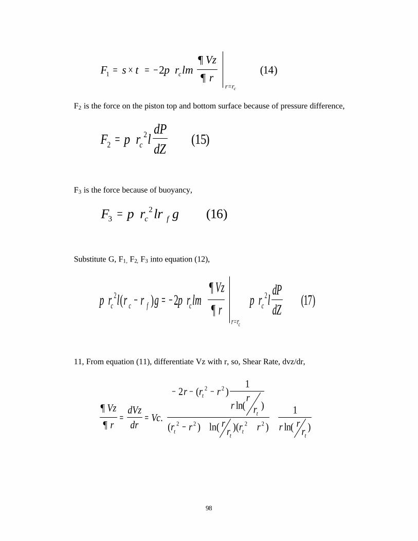
98
F s r lVz
rc
r rc
1 2 14= × = −
=
τ π µ∂
∂( )
F2 is the force on the piston top and bottom surface because of pressure difference,
F r ldPdZc2
2 15= π ( )
F3 is the force because of buoyancy,
F r l gc f32 16= π ρ ( )
Substitute G, F1, F2, F3 into equation (12),
π ρ ρ π µ∂
∂πr l g r l
Vz
rr l
dPdZc c f c
r r
c
c
2 22 17( ) ( )− = −
+
=
11, From equation (11), differentiate Vz with r, so, Shear Rate, dvz/dr,
∂
∂
Vz
rdVzdr
Vc
r r rr
rr
r r rr r r r r
r
t
t
tt
tt
= =
− − −
− + ++
.
( )ln( )
( ) ln( )( ) ln( )
21
1
2 2
2 2 2 2
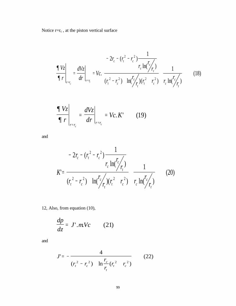
99
Notice r=rc , at the piston vertical surface
∂
∂
Vz
rdVzdr
Vc
r r rr r
r
r r rr r r r r
rr r r r
c t c
cc
t
t cc
tt c c
c
tc
c= =
= =
− − −
− + ++
.
( )ln( )
( ) ln( )( ) ln( )( )
21
118
2 2
2 2 2 2
∂
∂
Vz
rdVzdr
Vc Kr r r r
cc= =
= = . ' ( )19
and
K
r r rr r
r
r r rr r r r r
r
c t c
cc
t
t cc
tt c c
c
t
'
( )ln( )
( ) ln( )( ) ln( )( )=
− − −
− + ++
21
120
2 2
2 2 2 2
12, Also, from equation (10),
dpdz
J Vc= ' . . ( )µ 21
and
Jr r
rr
r rt cc
tt c
'( ) ln ( )
( )= −− + +
422
2 2 2 2

100
13. Now, substitute equation (19), (21) into equation (17), and simplify,
µρ ρ
=−
−
r g
Vc r J Kc c f
c
( )
( ' ')( )
223
14, We assume fluid is Newtonian fluid,
µρ ρ
=−
KVc
c f( )24
or ,
Vc Kc f
=−ρ ρ
µ( )25
and
Kr g
r J Kc
c
=−' '
( )2
26
15, For relative viscosity, according to equation (24), we can get it from the ratio of
terminal velocity of sample solution to that of pure CO2
Re cos ( )lative Vis ityVc
Vcsample
co
co
sample
= =µ
µ 2
2 27

101
16, For clearness, write the Shear Rate again, from equation (18),
Shear RatedVzdr
Vc
r r rr r
r
r rr
r r r rr
r
c t c
cc
t
t cc
tt c c
c
t
= =
− − −
− + ++
.
( )ln( )
( ) ln( )( ) ln( )( )
21
128
2 2
2 2 2 2

102
Example:
At 34Mpa (5000psi), 297K,
Pure CO2, viscosity uco2=1181.7up, density pf=0.9888g/cc
Falling cylinder, Aluminum density pc=2.7g/cc
Sample: 5wt% Copolymer (29%Styrene71%Fluoroacrylate)
Diameter of Glass Tube: 1.2500” (Dt)
Diameter of Piston: 1.2399” (Dc)
Terminal velocity of pure CO2: Vcsample=0.471cm/s
Terminal velocity of sample: Vcco2=0.004945cm/s
First, calculate rt, and rc
rt=Dt/2=1.2500inch*(2.54cm/inch)/2=1.5875cm
rc=Dc/2=1.2399inch*(2.54cm/inch)/2=1.5747cm
So, from equation (27),
Re cos. /
. /.lative Vis ity
VcVc
cm scm s
sample
co
co
sample
= = = =µ
µ 2
2 0 4710 004945
95 25
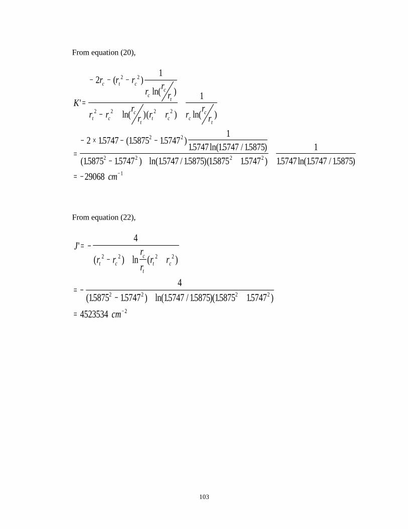
103
From equation (20),
K
r r rr r
r
r r rr r r r r
r
cm
c t c
cc
t
t cc
tt c c
c
t
'
( )ln( )
ln( )( ) ln( )
. ( . . ). ln( . / . )
( . . ) ln( . / . )( . . ) . ln( . / . )
=
− − −
− + ++
=− × − −
− + ++
= − −
21
1
2 15747 15875 157471
15747 15747 1587515875 15747 15747 15875 15875 15747
115747 15747 15875
29068
2 2
2 2 2 2
2 2
2 2 2 2
1
From equation (22),
Jr r
rr
r r
cm
t cc
tt c
'( ) ln ( )
( . . ) ln( . / . )( . . )
= −− + +
= −− + +
= −
4
415875 15747 15747 15875 15875 15747
4523534
2 2 2 2
2 2 2 2
2
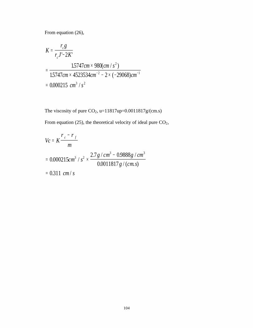
104
From equation (26),
Kr g
r J K
cm cm scm cm cm
cm s
c
c
=−
=×
× − × −
=
− −
' '
. ( / ). ( )
. /
2
15747 98015747 4523534 2 29068
0000215
2
2 1
3 2
The viscosity of pure CO2, u=11817up=0.0011817g/(cm.s)
From equation (25), the theoretical velocity of ideal pure CO2,
Vc K
cm sg cm g cm
g cm scm s
c f=
−
= ×−
=
ρ ρ
µ
0 0002152 7 0 9888
0 00118170 311
3 23 3
. /. / . /
. / ( . ). /

105
For pure CO2, from equation (28), shear rate is
Shear RatedVzdr
Vc
r r rr r
r
r rr
r r r rr
r
cm s
c t c
cc
t
t cc
tt c c
c
t
= =
− − −
− + ++
=
− × − −
− + +
.
( )ln( )
( ) ln( )( ) ln( )
. / .
. ( . . ). ln( .
. )
( . . ) ln( .. )( . . )
21
1
0311
2 15747 15875 157471
15747 1574715875
15875 15747 1574715875 15875 15747
2 2
2 2 2 2
2 2
2 2 2 2+
= − −
1
15747 1574715875
1
9045 1
. ln( .. ) cm
s
For copolymer sample, theoretical velocity (for ideal fluid),
Vs VcV
V
cm scm s
cm scm s
co
sample
= ×
= ×
=
2
0 3110 004945
0 4710 00327
. /. /
. /. /

106
For copolymer sample, shear rate
Shear RatedVzdr
Vc
r r rr r
r
r r rr r r r r
r
cm s
c t c
cc
t
t cc
tt c c
c
t
= =
− − −
− + ++
=
− × − −
− + +
.
( )ln( )
( ) ln( )( ) ln( )
. / .
. ( . . ). ln( .
. )
( . . ) ln( .. )( . .
21
1
000327
2 15747 15875 157471
15747 1574715875
15875 15747 1574715875 15875 15747
2 2
2 2 2 2
2 2
2 2 2 2 ) . ln( .. )
.
+
= − −
1
15747 1574715875
1
9505 1
cm
s
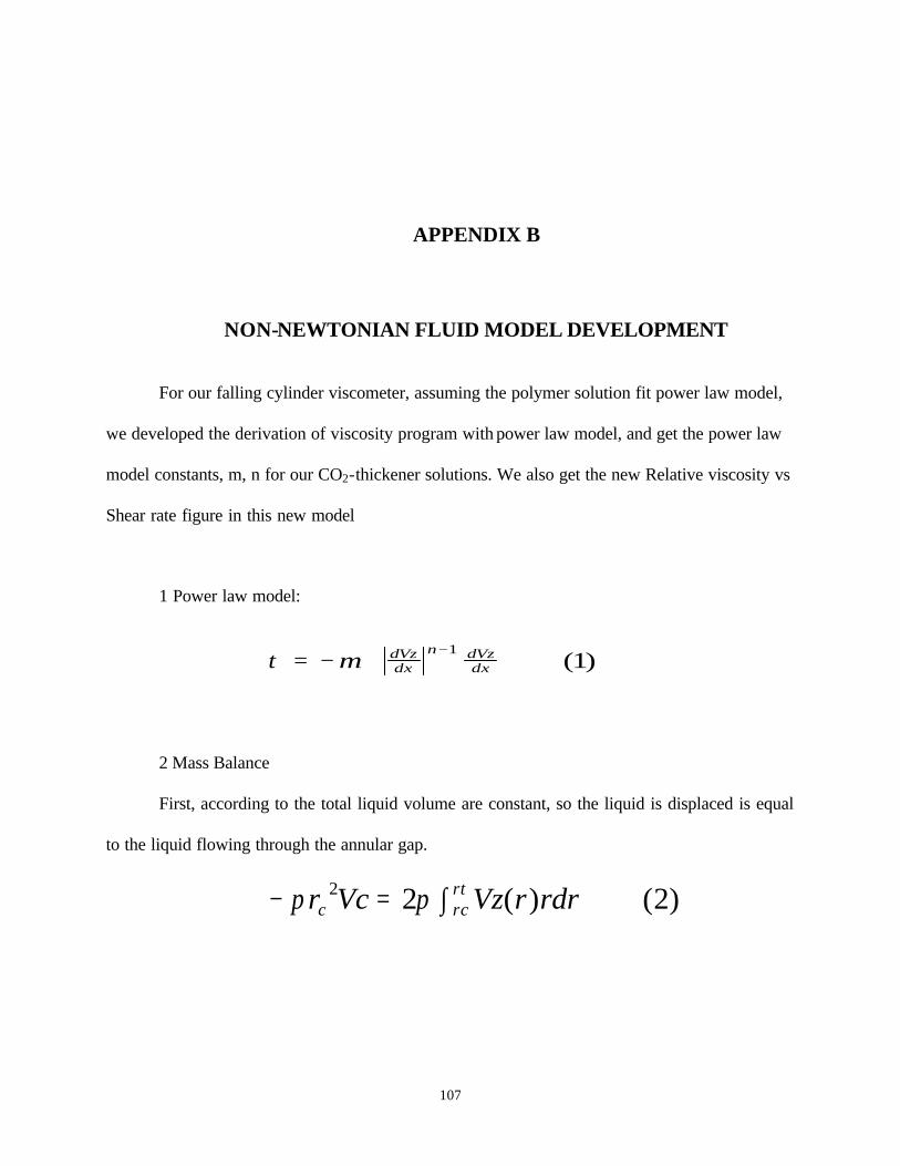
107
APPENDIX B
NON-NEWTONIAN FLUID MODEL DEVELOPMENT
For our falling cylinder viscometer, assuming the polymer solution fit power law model,
we developed the derivation of viscosity program with power law model, and get the power law
model constants, m, n for our CO2-thickener solutions. We also get the new Relative viscosity vs
Shear rate figure in this new model
1 Power law model:
τ = −−
m dVzdx
n dVzdx
11( )
2 Mass Balance
First, according to the total liquid volume are constant, so the liquid is displaced is equal
to the liquid flowing through the annular gap.
− = ∫π πr Vc Vz r rdrc rcrt2 2 2( ) ( )
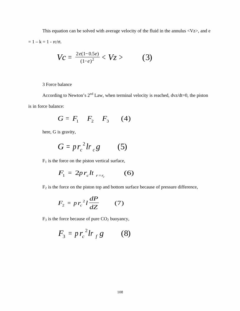
108
This equation can be solved with average velocity of the fluid in the annulus <Vz>, and e
= 1 – k = 1 - rc/rt.
Vc Vze ee= < >−
−2 1 0 5
1 2 3( . )( ) ( )
3 Force balance
According to Newton’s 2nd Law, when terminal velocity is reached, dvz/dt=0, the piston
is in force balance:
G F F F= + +1 2 3 4( )
here, G is gravity,
G r l gc c= π ρ2 5( )
F1 is the force on the piston vertical surface,
F r lc r rc1 2 6= =π τ ( )
F2 is the force on the piston top and bottom surface because of pressure difference,
F r ldPdZc2
2 7= π ( )
F3 is the force because of pure CO2 buoyancy,
F r l gc f32 8= π ρ ( )
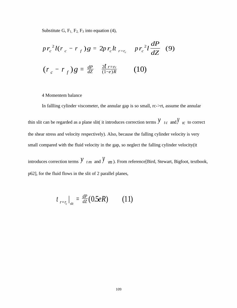
109
Substitute G, F1, F2, F3 into equation (4),
π ρ ρ π τ πr l g r l r ldPdZc c f c r r cc
2 22 9( ) ( )− = +=
( ) ( )( )ρ ρ τc f
dPdZ
r re Rg c− = + =
−21 10
4 Momentem balance
In fallling cylinder viscometer, the annular gap is so small, rc->rt, assume the annular
thin slit can be regarded as a plane slit( it introduces correction terms ψ τc and ψ vc to correct
the shear stress and velocity respectively). Also, because the falling cylinder velocity is very
small compared with the fluid velocity in the gap, so neglect the falling cylinder velocity(it
introduces correction terms ψ τm and ψ vm ). From reference[Bird, Stewart, Bigfoot, textbook,
p62], for the fluid flows in the slit of 2 parallel planes,
τ r rdPdZc slit
eR= =| ( . ) ( )0 5 11

110
5 From reference(Ashare),
τ τ ψ τr r r rc c= == 0 12( )
< > = < >Vz Vz v0 13ψ ( )
where, superscript 0 denotes that zeroth degree approximation. ψ τ and ψ v are the
correction for shear stress τ and velocity Vz because of the assumption of plane slit and
stationary falling cylinder, and ψ ψ ψτ τ τ= ×c m , ψ ψ ψv vc vm= ×
ψ v e e e= − − +1 14320
2 135
4 ( )
ψ τ = −−
1 0 51 15. ( )e
e
6 dP/dZ,
From equation 10, 11, and 12, we can get dP/dZ
dPdZ
gc fe
e=
−
+ −
( )( )
ρ ρ
ψ τ1 116

111
7 Power law fluid
From reference (Fredrickson and Bird, Ind. Eng. Chem., 50, 347(1958)), the average
velocity of the fluid in the plane slit,
< > = +Vz slitpeRmL
s eRs| ( ) ( )( )
∆2 2 2 17
where, s=1/n
8 Final equation
Combine equation(3, 13, 16, 17), we can get:
[ ]Vc e ee
eRS
eRm
sv
gs
c fee
= −− +
−
+ −
2 1 0 51 2 2 2 12
118( . )
( ) ( )( )
. .( ) . . ( )ψρ ρ
ψ τ
9 Model constants
In reference[Ashare], they did experiment with different cylinder(different cylinder
density ρc, the same size), so, the same e, it is easy to get constant s, if one log both sides of the
final equation, get straight line of logVc vs. Log[ ]( )ρ ρ
ψ τ
c fe
e
g−
+ −1 1 , and the sloap is the s, then
substitued a pair of data(Vc, ρc), can get constant m.
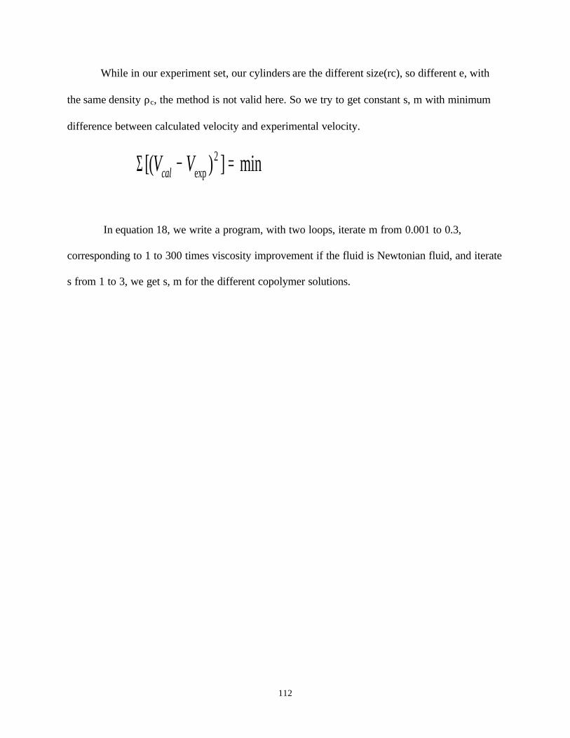
112
While in our experiment set, our cylinders are the different size(rc), so different e, with
the same density ρc, the method is not valid here. So we try to get constant s, m with minimum
difference between calculated velocity and experimental velocity.
Σ [( ) ] minexpV Vcal − =2
In equation 18, we write a program, with two loops, iterate m from 0.001 to 0.3,
corresponding to 1 to 300 times viscosity improvement if the fluid is Newtonian fluid, and iterate
s from 1 to 3, we get s, m for the different copolymer solutions.
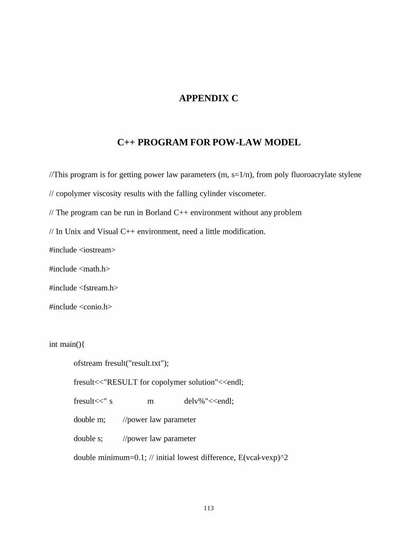
113
APPENDIX C
C++ PROGRAM FOR POW-LAW MODEL
//This program is for getting power law parameters (m, s=1/n), from poly fluoroacrylate stylene
// copolymer viscosity results with the falling cylinder viscometer.
// The program can be run in Borland C++ environment without any problem
// In Unix and Visual C++ environment, need a little modification.
#include <iostream>
#include <math.h>
#include <fstream.h>
#include <conio.h>
int main(){
ofstream fresult("result.txt");
fresult<<"RESULT for copolymer solution"<<endl;
fresult<<" s m delv%"<<endl;
double m; //power law parameter
double s; //power law parameter
double minimum=0.1; // initial lowest difference, E(vcal-vexp)^2
114
//terminal velocity(cm/s) for falling cylinder in (29%FA) soln.
//double vcexp[]={0.0023, 0.00388, 0.02536, 0.118,
// 0.004104, 0.004945, 0.015};
//double vcexp[]={0.00479, 0.01356, 0.05091, 0.33}; //3wt%
//double vcexp[]={0.03022, 0.03597, 0.1957,
// 0.84, 0.01325, 0.1334, 0.35}; //1wt%
//double vcexp[]={0.04997, 0.174, 0.093,
// 0.362, 1.08}; //0.2wt%
double vcexp[]={0.06, 0.15}; //0.1wt%
double vccal[2]; //calcuated falling cylinder velocity(cm/s)
//falling cylinder diameter(inch)
//double rc[]={1.2438, 1.2428, 1.2399, 1.2311,
// 1.2438, 1.2399, 1.2339}; //5wt%
//double rc[]={1.2438, 1.2428, 1.2399, 1.2311}; //3wt%
//double rc[]={1.2438, 1.2428, 1.2399, 1.2311,
// 1.2438, 1.2399, 1.2339}; //1wt%
//double rc[]={1.245, 1.2428, 1.2438,
// 1.2399, 1.2339}; //0.2wt%
double rc[]={1.245, 1.2428}; //0.1wt%
double rt=1.25; //tube diameter(inch)
115
double R=rt*2.54/2; //tube radius (cm)
double deltapg=(2.7-0.9888)*980; //(p0-p)*g, p(density)
for (m=0.001; m<0.3; m+=0.001){
for (s=1; s<3.0; s+=0.01){
double sum=0;
for (int i=0; i<2; i++){ // for different cylinder
double e=1-rc[i]/rt;
double phiv=1-e-3/20*e*e;
double phit=(1-0.5*e)/(1-e);
//cout<<"e:"<<e<<" phiv"<<phiv<<" phit:"<<phit
//<<" s:"<<s<<" m:"<<m<<"deltapg:"<<deltapg<<endl;
vccal[i]=2*e*(1-0.5*e)/(1-e)/(1-e)*e*R/2/(s+2)
*exp(s*log(e*R/2/m*deltapg/(1+e/(1-e)*phit)))
*phiv;
// cout<<”debug:”<<endl;
//cout<<"vccal["<<i<<"]:"<<vccal[i]<<endl;
fresult<<s<<" "<<m<<" "
<<((vccal[i]-vcexp[i])*100)<<endl;
sum+=(vccal[i]-vcexp[i])*(vccal[i]-vcexp[i]);
}
fresult<<" Sum: "<<sum<<endl;
if(sum<minimum) {
minimum= sum;

116
cout<<"m: "<<m<<"s: "<<s<<" Sum: "<<sum<<endl;
}
}//end of for(s)
}//end of for(m)
cout<<"It is done!";
getch();
return 0;
}
117
APPENDIX D
MATLAB PROGRAM FOR FALLING CYLINDER VISCOMETER CALIBRATION
% The following is the matlab program, used for falling cylinder viscometer calibration.
% the function is for get Vct of different piston,
% also the dvzdr close to the piston
% input the piston diameter(inch), co2 density(g/cm3), co2 viscosity(g/cm/s)
function vct=dvzdr3(piston,density,viscosity)
rc0=piston*2.54/2.0; %change to cm, radium
rt=1.250*2.54/2.0; %change to cm, radium
pf=density; % density of co2
pc=2.7; %density of aluminum piston
pc_pf=pc-pf; %density difference
g=980; %gravity constant
dr=(rt-rc0)/20;
rt0=rc0+(rt-rc0)/20*19;
rc=rc0:dr:rt0;
dvzdr=zeros(20); %initiate dvzdr[21]
for l=1:20
gap(l)=rt-rc(l);
118
dem0(l)=log(rc(l)/rt)*(rt^2+rc(l)^2)+(rt^2-rc(l)^2); % common term in downstairs
j1(l)=-4/(log(rc(l)/rt)*(rt^2+rc(l)^2)+(rt^2-rc(l)^2)); % one term in K
k1(l)=(-2*rc(l)-(rt^2-rc(l)^2)/rc(l)/log(rc(l)/rt))/(log(rc(l)/rt)*(rt^2+rc(l)^2)+(rt^2-
rc(l)^2))+1/rc(l)/log(rc(l)/rt);
k(l)=rc(l)*g/(rc(l)*j1(l)-2*k1(l)); % get K
vct(l)=k(l)*pc_pf/viscosity; % terminal velocity
r(l)=rc(l); % calculate the point close to piston
dvzdrc(l)=vct(l)*((-2*r(l)-1/r(l)/log(rc(l)/rt)*(rt^2-rc(l)^2))/(rt^2-
rc(l)^2+log(rc(l)/rt)*(rt^2+rc(l)^2))+1/r(l)/log(rc(l)/rt));
end %get dvzdr
% rinch=r*2/2.54 %return to inch unit
gapmin=gap+0.00015*2.54
gapmax=gap-0.00015*2.54
vct % show terminal velocity cm/s
dvzdrc % show dvzdr close to the piston
plot(gap,dvzdrc)
title('shear rate vs gap');
xlabel('gap (cm)');
ylabel('dvz/dr (s-1)');
119
deltagap1=[0.0031,0.0031,0.0031];
deltavct1=[0.198,0.188,0.183];
deltagap2=[0.00295,0.0031,0.00325];
deltavct2=[0.188,0.188,0.188];
deltagap3=[0.00505,0.00505,0.00505];
deltavct3=[0.641,0.568,0.543];
deltagap4=[0.0049,0.00505,0.0052];
deltavct4=[0.568,0.568,0.568];
deltagap5=[0.00805,0.00805,0.00805];
deltavct5=[1.41,1.3,1.02];
deltagap6=[0.0079,0.00805,0.0082];
deltavct6=[1.3,1.3,1.3];
deltagap1=deltagap1*2.54;
deltagap2=deltagap1*2.54;
deltagap3=deltagap1*2.54;
deltagap4=deltagap1*2.54;
deltagap5=deltagap1*2.54;
deltagap6=deltagap1*2.54;
deltagap=[0.0031,0.0031,0.0031,0.00325,0.0031,0.00295,0.00505,0.00505,0.00505,0.0052,
0.00505,0.0049,0.00805,0.00805,0.00805,0.00820,0.00805,0.0079];
120
deltavct=[0.198,0.188,0.183,0.188,0.188,0.188,0.641,0.568,0.543,0.568,0.568,0.568,1.41,1.3,
1.02,1.3,1.3,1.3];
deltagap=deltagap*2.54;
plot(gap,vct,gapmax,vct,gapmin,vct,deltagap,deltavct,'*')
title('ideal terminal velocity of different piston');
xlabel('gap (cm)');
ylabel('Vct (cm/s)');

BIBLIOGRAPHY

122
BIBLIOGRAPHY
1. Taber, J. J., Martin, F. D., Seright, R. S., “EOR screening criteria revisited---part1: introduction to screening criteria and enhanced recovery field projects”, SPE reservoir engineering, p189-198, August, 1997. 2. Moritis, G., Annual Production Report; Oil and Gas Journal, Vol. 88, No. 17, p49-82, 1990. 3. Enick, R.M., “A Literature Review of Attempts to Increase the Viscosity of Dense Carbon Dioxide”, US DOE NETL report DE-AP26-97FT25356, Oct. 1998, www.netl.doe.gov 4. Blackwell, R.J., Terry, W.M, Rayne, J.R., Lindley, D.C., and Henderson, J.R., “Recovery of oil by displacement with water-solvent mixtures,” Trans. AIME 219, 293-300, 1960. 5. Caudle, B.H. and Dyes, A.B., “Improving miscible displacement by Gas-Water Injection,” Trans. AIME 213, 281-284, 1958. 6. Llave, F.M., Chung, T-H., Burchfield, T.E., “Use of entrainers in improving mobility control of supercritical CO2”, SPE reservoir engineering, p47-51, February, 1990. 7. Llave, F.M., Chung, T-H, Burchfield, T.E., “the use of entrainers in improving mobility control of supercritical carbon dioxide”, SPE 17344. May 1988. 8. Terry, R.E., Zaid, A., Angelos, C., and Whitman, D.L., “polymerization in supercritical CO2 to improve CO2/Oil mobility ratios”, SPE 16270, 1987. 9. Lancaster, G. W., Barrientos, C., Li, E., Greenhorn, R. C., “high phase volume liquid CO2 fracturing fluids”, Petroleum Society of CIM, paper NO. 87-38-71, 1987. 10. Lancaster, G., Sinal, M., “Liquid Carbon Dioxide Fracturing: Advantages and Disadvantages”, CIM 86-37-69 (July 1986). 11. Heller, J.P., Dandge, D.K., Card, R.J., Donaruma, L.G., “Direct thickeners for mobility control of CO2 floods”, Society of Petroleum Engineers Journal, p679-686, October, 1985. 12. Dandge, D.K., Taylor, C., Heller, J.P., Wilson, K.V., and Brumley, N., “associate organotin polymers”, J. of Macromolecular Science, Chem A 26 #18 (1989) 1451-1461. 13. Martin, F. and Heller J., PRRC 90-20, June 1990.

123
14. Davis, B. W., U.S. Patent 4,852,651, 1989 15. Davis, B.W., U.S. Patent 4,989,674, 1991. 16. Davis, B.W., U.S. Patent 5,080,169, 1992. 17. Davis, B.W., U.S. Patent 5,123,486, 1992. 18. Bae, J.H. and Irani, C.A., “A laboratory investigation of thickened CO2 process”, SPE 20467, p73-78, 1990. 19. Harris, T.V., Irani, C.A., and Pretzer, W.R., U.S. Patent 4,913,235, 1990. 20. McClain, J.B., Betts, D.E., Canelas, D.A., Samulski, E.T., DeSimone, J.M., “Characterization of polymers and amphiphiles in supercritical CO2 using small angle neutron scattering and viscometry”, Spring meeting of the ACS, Division of polymeric materials science and engineering, p234-235, New Orleans, LA, 1996. 21. Guan, Z., McClain, J.B., Samulski, E.T., DeSimone, J.M., “fluorocarbon/Hydrocarbon block copolymers for CO2 viscosity enhancement”, Polymer preprint, V. 35, No. 1, p725-6, 1994. 22. McHugh, M.A., Krukonis, V.J., Supercritical Fluid Extraction: Principle and Practice, 2nd ed., Butterworths: Stoneham, MA, 1994. 23. Krukonis, V.J., J. Polym. News, V 11, 7, 1985. 24. Ghenciu G. Ph.D. dissertation, Department of Chemical and Petroleum Engineering, University of Pittsburgh. Ann Arbor: UMI Dissertation Services, 1998. 25. Rindfleisch, F., DiNoia, T.P., and McHugh, M.A., “solubility of polymers and copolymers in supercritical CO2”, J. Phys. Chem., 100, 15581-15587, 1996. 26. Sarbu, T., Styranec, T., Beckman E. J., “non-fluorous polymers with very high solubility in supercrit ical CO2 down to low pressures”, Nature, V 405, p165-168, May, 2000. 27. O’Neill, M.L., Cao, Q., Fang, M., Johnston, K.P., “Solubility of homopolymers and copolymers in carbon dioxide”, Ind. Eng. Chem. Res., 37, 3067-3079, 1998. 28. Conway S. E., Byun H-S, McHugh M.A., Wang J.D., Mandel F.S., J. Appl Polym Sci 2001; 80: 1155-1161 29. Styranec, T., M.S. Thesis, University of Pittsburgh, 2000.
124
30. Huang, Z., Shi, C., Xu., J., Kilic, S., Enick, R.M., Beckman, E.J., “Enhancement of the Viscosity of Carbon Dioxide Using Styrene/Fluoroacrylate Copolymers”, Macromolecules, 33(15), p5437-5442, 2000. 31. Simion, C., Christina, B.J., Kathryn L.B., Krzysztof M., “ Polymerization of Acrylates by Atom Transfer radical Polymerization Homopolymerization of 2-Hydroxyethyl Acrylate”, Journal of Polymer Science: Part A: Polymer Chemistry, Vol 36, p1417-1424 (1998) 32. Xia, J., Paik, H.J., Matyjaszewski, K., “ Polymerization of Vinyl Acetate Promoted by Iron Complexes” Macromolecues, Vol 32, p8310-8314, 1999. 33. Lawaczeck, F. Z., Ver. Deut. Ing., 63, p677, 1919. 34. Lohrenz, J., Swift, G. W., Kurata, F., “an experimentally verified theoretical study of the falling cylinder viscometer”, A.I.Ch.E, V. 6, No. 4, p547-550, 1960. 35. Lohrenz, J., Kurata, F., “design and eva luation of a new body for falling cylinder viscometers”, A.I.Ch.E., V.8, No. 2, p190-194, 1962. 36. Eichstadt, F. J., Swift, G. W., “theoretically analysis of the falling cylinder viscometer for power law and bingham plastic fluids”, A.I.Ch.E. V12, No. 6, p1179-1183, 1966. 37. Ashare, E., Bird, R. B., “falling cylinder viscometer for non-newtonian fluids”, A.I.Ch.E. V11, No. 5, p910-916, 1965. 38. Barrage, T. C., M.S. Thesis, University of Pittsburgh, 1985. 39. Iezzi, A., M.S. Thesis, University of Pit tsburgh, 1989. 40. Shi, C., Huang. Z.; Kilic, S., Xu, J., Enick, R. M., Beckman, E. J., Carr, A., J., Melendez, R., E., Hamilton, A. D., Science, 286, p1540, 1999. 41. Kiran, E., Yeo, S., “Viscosity reduction of polystyrene solution in toluene with supercritical carbon dioxide”, Macromolecules, V32 (21), p7325-7328, 1999. 42. Enick, R., “The effect of hydroxy aluminum disoaps on the viscosity of light alkanes and carbon dioxide”, SPE 21026, 149-156, 1991. 43. Hunter, C. A. and Sanders J. K. M., “The nature of π-π interactions”, J. Am. Chem. Soc. V112, p5525-5534, 1990. 44. Drohmann C., Beckman E.J., J. Supercrit Fluid 2002, 22: 103:110 45. DeSimone J.M., Guan Z., Elsbernd C.S., Science 1992, 257:945-947 46. Blasig A, Shi C., Enick R., Thies M., Ind Eng Chem Res in press
125
47. Mawson S., Johnston K.P., Combes J.R., DeSimone J.M., Macromolecules 1995, 28:3182-3191. 48. Hsiao Y.L, Maury E.E., DeSimone J.M., Mawson S., Johnston K.P., Macromolecules 1995, 28:8159-8166 49. Canelas D.A., Betts D.E., Desimone J.M., Yates M.Z., Johnston K.P., Macromolecules 1998, 31:6794-6805 50. Meilchen M.A., Hasch B.M., McHugh M.A., Macromolecules,1991, 24:4874-4882 51. Mertdogan C. A., Byun H. S., McHugh M.A., Tuminello W.H., Macromolecules 1996, 29:6548-6555 52. Allen G., Baker C.H., Polymer 1965, 6: 181-191 53. Irani C.A., Cozewith C. J Appl Polym Sci 1986, 31: 1879-1899 54. Lee S. H., Lostracco M.A., Hasch B.M., McHugh M.A, J Phys Chem 1994, 98: 4055-4060 55. Wallen, S., “Cooperative Hydrogen Bonds in CO2 and Implications for Solvation,” presentation at the 10th International Symposium and Exhibit on Supercritical Fluid Chromatography, Extraction, and Processing, August 19-22, 2001, Myrtle Beach, SC. 56. Lora M., Lim J.S., McHugh M.A., J Phys Chem B 1999, 103:2818-2822 57. Bayraktar Z., Kiran E., J. Appl. Polym Sci. 2000, 75:1397-1403.