capital structure advanced issues - wz.uw.edu.pl · net operating profit after taxes ... financial...

© 2017 Cengage Learning. All Rights Reserved. May not be copied, scanned, or duplicated, in whole or in part, except for use as

permitted in a license distributed with a certain product or service or otherwise on a password-protected website for classroom use. 1

Chapter 21

Dynamic Capital Structures and Corporate Valuation



Topics in Chapter

MM models, with and without corporate

taxes

Miller model, with corporate and

personal taxes

Compressed adjusted present value model

Equity as an option

MM proofs



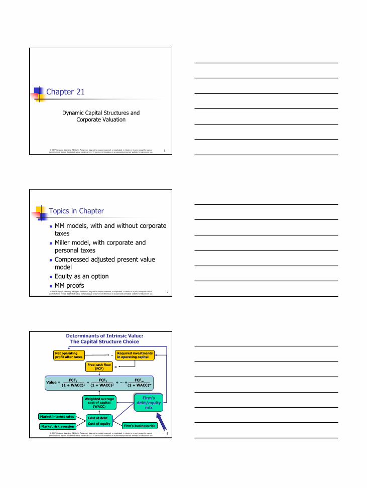
Value = + + ··· + FCF1 FCF2 FCF∞

(1 + WACC)1 (1 + WACC)∞ (1 + WACC)2

Free cash flow (FCF)

Market interest rates

Firm’s business risk Market risk aversion

Firm’s debt/equity

mix

Cost of debt

Cost of equity

Weighted average cost of capital

(WACC)

Net operating profit after taxes

Required investments in operating capital

−

=

Determinants of Intrinsic Value: The Capital Structure Choice



Who are Modigliani and Miller (MM)?

They published theoretical papers that changed the way people thought about financial leverage.

They won Nobel prizes in economics because of their work.

MM’s papers were published in 1958 and 1963. Miller had a separate paper in 1977. The papers differed in their assumptions about taxes.



What assumptions underlie the MM and Miller Models?

Firms can be grouped into

homogeneous classes based on business risk.

Investors have identical expectations about firms’ future earnings.

There are no transactions costs.

No agency or financial distress costs. (More...)



All debt is riskless, and both individuals

and corporations can borrow unlimited amounts of money at the risk-free rate.

All cash flows are perpetuities. This implies perpetual debt is issued, firms

have zero growth, and expected EBIT is constant over time.

What assumptions underlie the MM and Miller Models?


permitted in a license distributed with a certain product or service or otherwise on a password-protected website for classroom use.

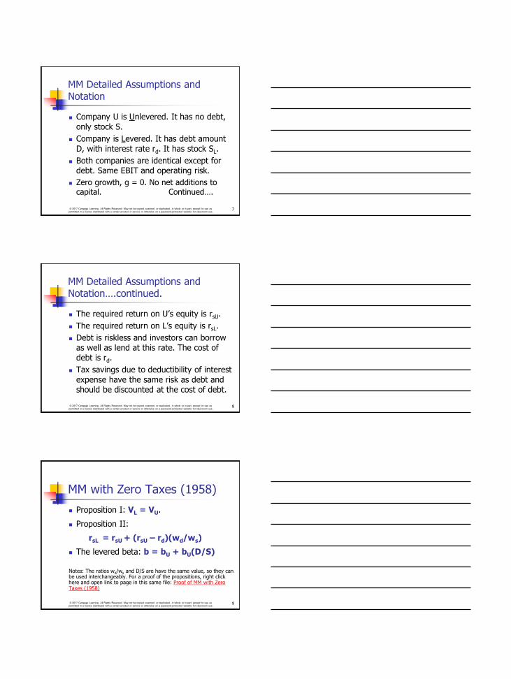
MM Detailed Assumptions and Notation

Company U is Unlevered. It has no debt,

only stock S.

Company is Levered. It has debt amount

D, with interest rate rd. It has stock SL.

Both companies are identical except for debt. Same EBIT and operating risk.

Zero growth, g = 0. No net additions to capital. Continued….

7



MM Detailed Assumptions and Notation….continued.

The required return on U’s equity is rsU.

The required return on L’s equity is rsL.

Debt is riskless and investors can borrow as well as lend at this rate. The cost of

debt is rd.

Tax savings due to deductibility of interest

expense have the same risk as debt and should be discounted at the cost of debt.

8



MM with Zero Taxes (1958)

Proposition I: VL = VU.

Proposition II:

rsL = rsU + (rsU – rd)(wd/ws)

The levered beta: b = bU + bU(D/S)

Notes: The ratios wd/ws and D/S are have the same value, so they can be used interchangeably. For a proof of the propositions, right click here and open link to page in this same file: Proof of MM with Zero Taxes (1958)

9



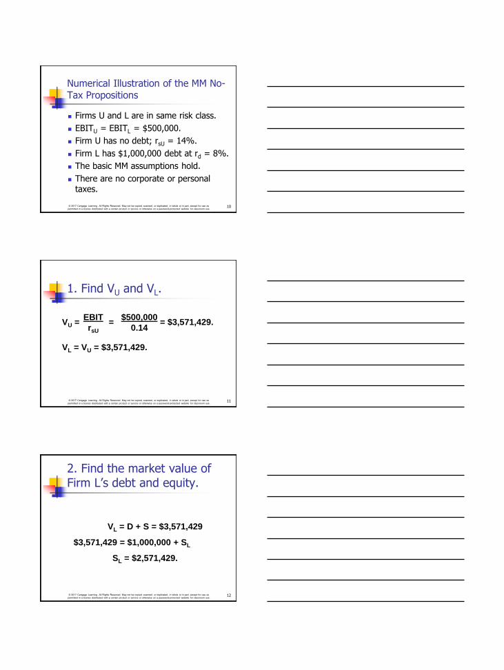
Numerical Illustration of the MM No-Tax Propositions

Firms U and L are in same risk class.

EBITU = EBITL = $500,000.

Firm U has no debt; rsU = 14%.

Firm L has $1,000,000 debt at rd = 8%.

The basic MM assumptions hold.

There are no corporate or personal taxes.



VU = = = $3,571,429.

VL = VU = $3,571,429.

EBIT

rsU

$500,000

0.14

1. Find VU and VL.



VL = D + S = $3,571,429

$3,571,429 = $1,000,000 + SL

SL = $2,571,429.

2. Find the market value of Firm L’s debt and equity.



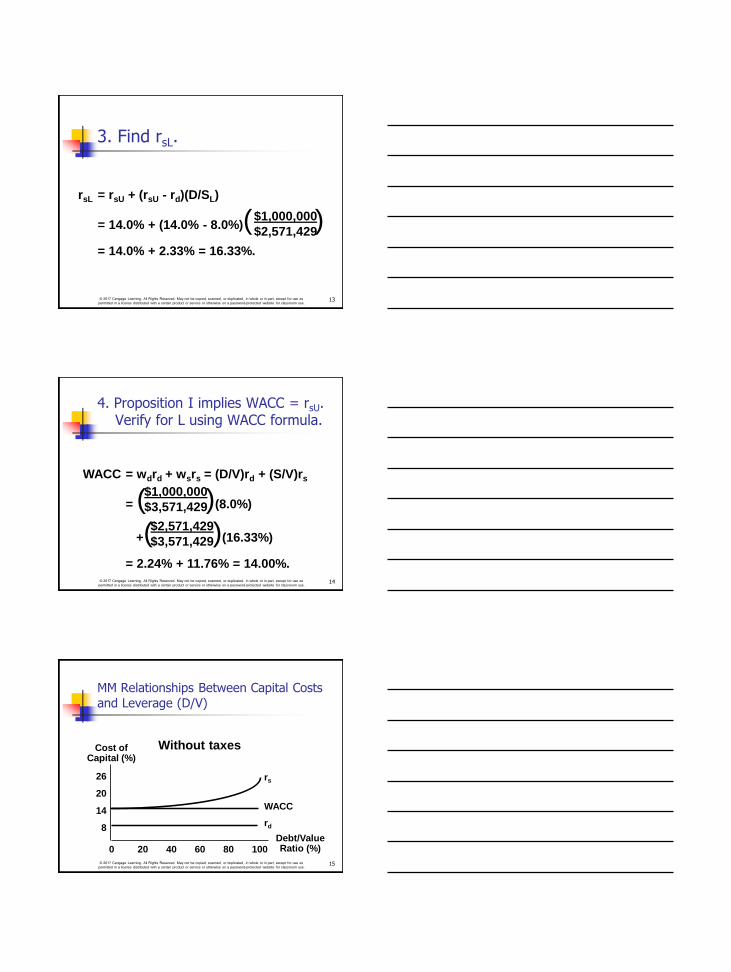
rsL = rsU + (rsU - rd)(D/SL)

= 14.0% + (14.0% - 8.0%)( ) = 14.0% + 2.33% = 16.33%.

$1,000,000

$2,571,429

3. Find rsL.



WACC = wdrd + wsrs = (D/V)rd + (S/V)rs

= ( )(8.0%)

+( )(16.33%) = 2.24% + 11.76% = 14.00%.

$1,000,000

$3,571,429

$2,571,429

$3,571,429

4. Proposition I implies WACC = rsU. Verify for L using WACC formula.



Without taxes Cost of Capital (%)

26

20

14

8

0 20 40 60 80 100 Debt/Value Ratio (%)

rs

WACC

rd

MM Relationships Between Capital Costs

and Leverage (D/V)



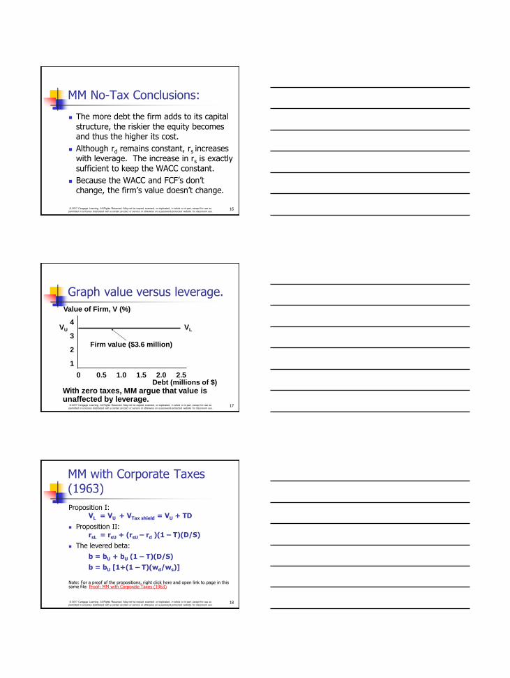
MM No-Tax Conclusions:

The more debt the firm adds to its capital

structure, the riskier the equity becomes and thus the higher its cost.

Although rd remains constant, rs increases with leverage. The increase in rs is exactly

sufficient to keep the WACC constant.

Because the WACC and FCF’s don’t change, the firm’s value doesn’t change.



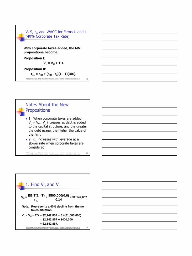
Value of Firm, V (%)

4

3

2

1

0 0.5 1.0 1.5 2.0 2.5 Debt (millions of $)

VL VU

Firm value ($3.6 million)

With zero taxes, MM argue that value is unaffected by leverage.

Graph value versus leverage.



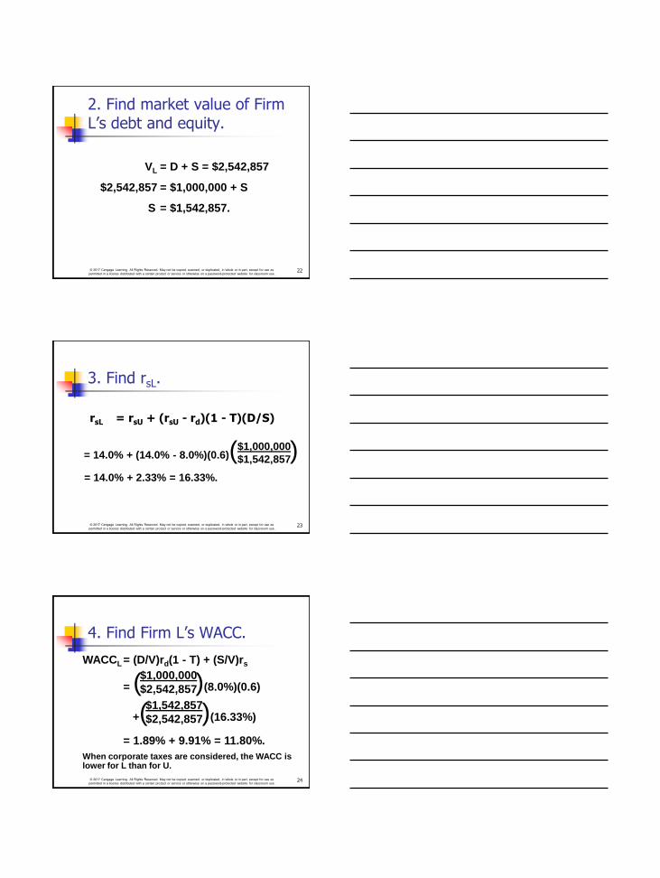
MM with Corporate Taxes (1963)

Proposition I: VL = VU + VTax shield = VU + TD

Proposition II: rsL = rsU + (rsU – rd )(1 – T)(D/S)

The levered beta:

b = bU + bU (1 – T)(D/S)

b = bU [1+(1 – T)(wd/ws)]

Note: For a proof of the propositions, right click here and open link to page in this same file: Proof: MM with Corporate Taxes (1963)

18



With corporate taxes added, the MM

propositions become: Proposition I:

VL = VU + TD. Proposition II:

rsL = rsU + (rsU - rd)(1 - T)(D/S).

V, S, rs, and WACC for Firms U and L (40% Corporate Tax Rate)



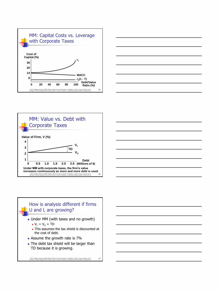
Notes About the New Propositions

1. When corporate taxes are added,

VL ≠ VU. VL increases as debt is added to the capital structure, and the greater

the debt usage, the higher the value of the firm.

2. rsL increases with leverage at a slower rate when corporate taxes are considered.



Note: Represents a 40% decline from the no

taxes situation.

VL = VU + TD = $2,142,857 + 0.4($1,000,000)

= $2,142,857 + $400,000

= $2,542,857.

VU = = = $2,142,857. EBIT(1 - T)

rsU

$500,000(0.6)

0.14

1. Find VU and VL.



VL = D + S = $2,542,857

$2,542,857 = $1,000,000 + S

S = $1,542,857.

2. Find market value of Firm L’s debt and equity.



= 14.0% + (14.0% - 8.0%)(0.6)( ) = 14.0% + 2.33% = 16.33%.

$1,000,000

$1,542,857

3. Find rsL.

rsL = rsU + (rsU - rd)(1 - T)(D/S)



WACCL = (D/V)rd(1 - T) + (S/V)rs

= ( )(8.0%)(0.6)

+( )(16.33%)

= 1.89% + 9.91% = 11.80%.

When corporate taxes are considered, the WACC is lower for L than for U.

$1,000,000

$2,542,857

$1,542,857

$2,542,857

4. Find Firm L’s WACC.



Cost of Capital (%)

26

20

14

8

0 20 40 60 80 100 Debt/Value Ratio (%)

rs

WACC

rd(1 - T)

MM: Capital Costs vs. Leverage with Corporate Taxes



Under MM with corporate taxes, the firm’s value increases continuously as more and more debt is used.

Value of Firm, V (%)

4

3

2

1

0 0.5 1.0 1.5 2.0 2.5 Debt

(Millions of $)

VL

VU

TD

MM: Value vs. Debt with Corporate Taxes



How is analysis different if firms U and L are growing?

Under MM (with taxes and no growth)

VL = VU + TD

This assumes the tax shield is discounted at the cost of debt.

Assume the growth rate is 7%

The debt tax shield will be larger than

TD because it is growing.



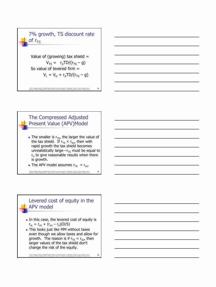
7% growth, TS discount rate of rTS

Value of (growing) tax shield =

VTS = rdTD/(rTS – g)

So value of levered firm =

VL = VU + rdTD/(rTS – g)



The Compressed Adjusted Present Value (APV)Model

The smaller is rTS, the larger the value of

the tax shield. If rTS < rsU, then with rapid growth the tax shield becomes

unrealistically large—rTS must be equal to rU to give reasonable results when there is growth.

The APV model assumes rTS = rsU.



Levered cost of equity in the APV model

In this case, the levered cost of equity is

rsL = rsU + (rsU – rd)(D/S)

This looks just like MM without taxes

even though we allow taxes and allow for growth. The reason is if rTS = rsU, then

larger values of the tax shield don't change the risk of the equity.



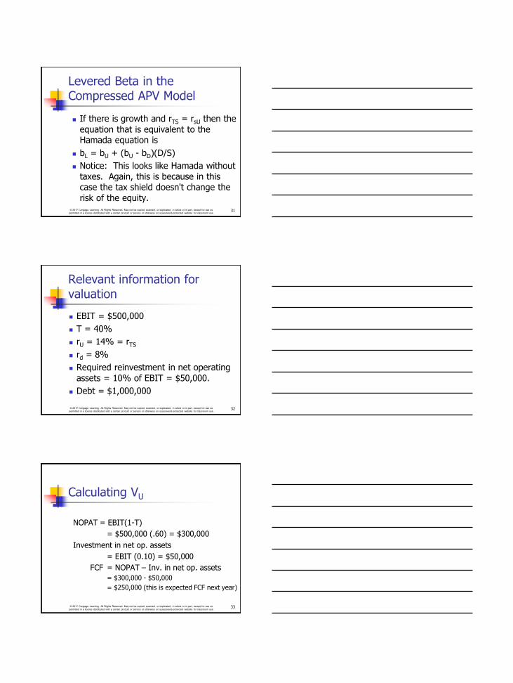
Levered Beta in the Compressed APV Model

If there is growth and rTS = rsU then the equation that is equivalent to the Hamada equation is

bL = bU + (bU - bD)(D/S)

Notice: This looks like Hamada without

taxes. Again, this is because in this case the tax shield doesn't change the

risk of the equity.



Relevant information for valuation

EBIT = $500,000

T = 40%

rU = 14% = rTS

rd = 8%

Required reinvestment in net operating assets = 10% of EBIT = $50,000.

Debt = $1,000,000



Calculating VU

NOPAT = EBIT(1-T)

= $500,000 (.60) = $300,000

Investment in net op. assets

= EBIT (0.10) = $50,000

FCF = NOPAT – Inv. in net op. assets

= $300,000 - $50,000

= $250,000 (this is expected FCF next year)



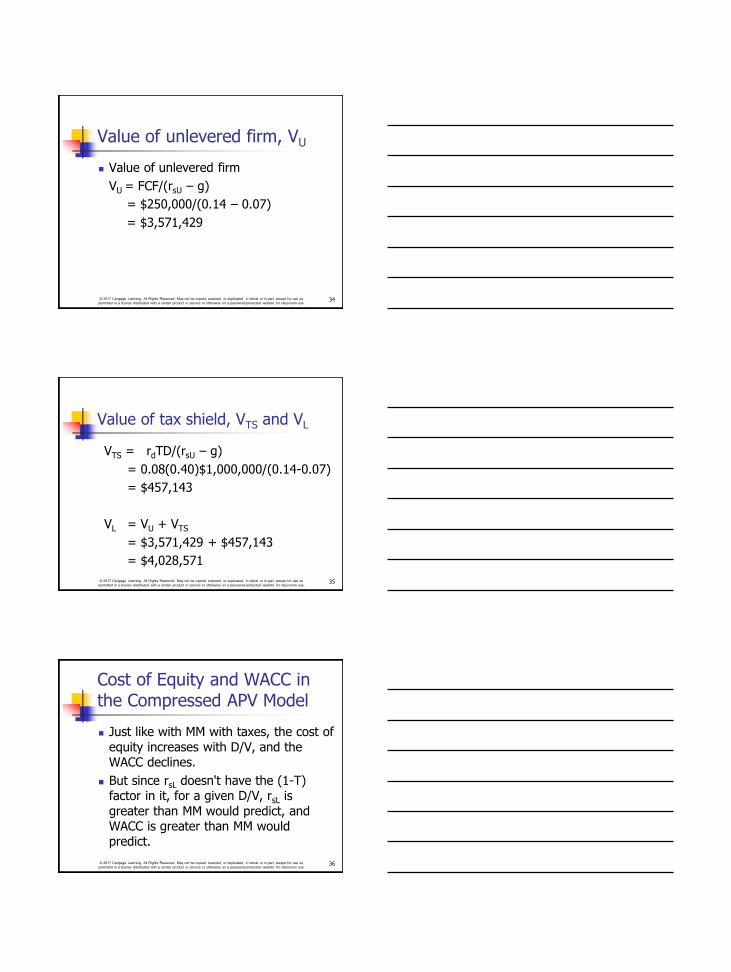
Value of unlevered firm, VU

Value of unlevered firm

VU = FCF/(rsU – g)

= $250,000/(0.14 – 0.07)

= $3,571,429



Value of tax shield, VTS and VL

VTS = rdTD/(rsU – g)

= 0.08(0.40)$1,000,000/(0.14-0.07)

= $457,143

VL = VU + VTS

= $3,571,429 + $457,143

= $4,028,571



Cost of Equity and WACC in the Compressed APV Model

Just like with MM with taxes, the cost of

equity increases with D/V, and the WACC declines.

But since rsL doesn't have the (1-T) factor in it, for a given D/V, rsL is

greater than MM would predict, and WACC is greater than MM would predict.



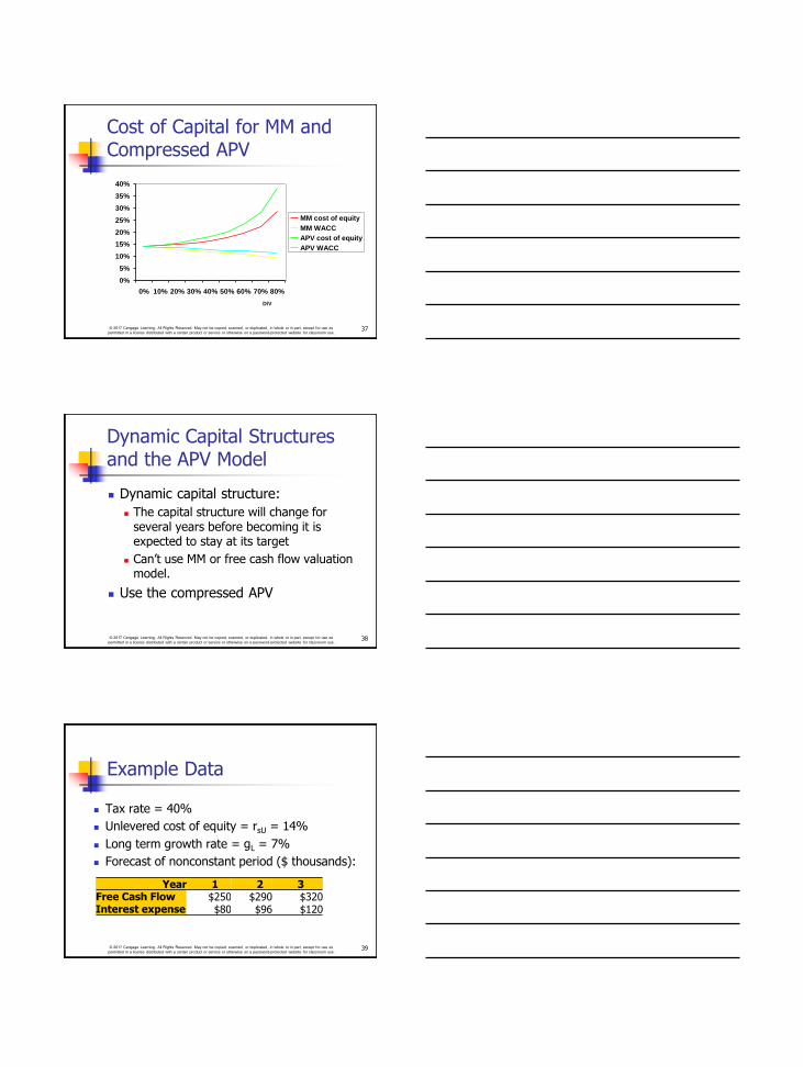
Cost of Capital for MM and Compressed APV

0%

5%

10%

15%

20%

25%

30%

35%

40%

0% 10% 20% 30% 40% 50% 60% 70% 80%

D/V

MM cost of equity

MM WACC

APV cost of equity

APV WACC



Dynamic Capital Structures and the APV Model

Dynamic capital structure:

The capital structure will change for several years before becoming it is expected to stay at its target

Can’t use MM or free cash flow valuation model.

Use the compressed APV

38



Example Data

Year 1 2 3

Free Cash Flow $250 $290 $320

Interest expense $80 $96 $120

Tax rate = 40%

Unlevered cost of equity = rsU = 14%

Long term growth rate = gL = 7%

Forecast of nonconstant period ($ thousands):

39



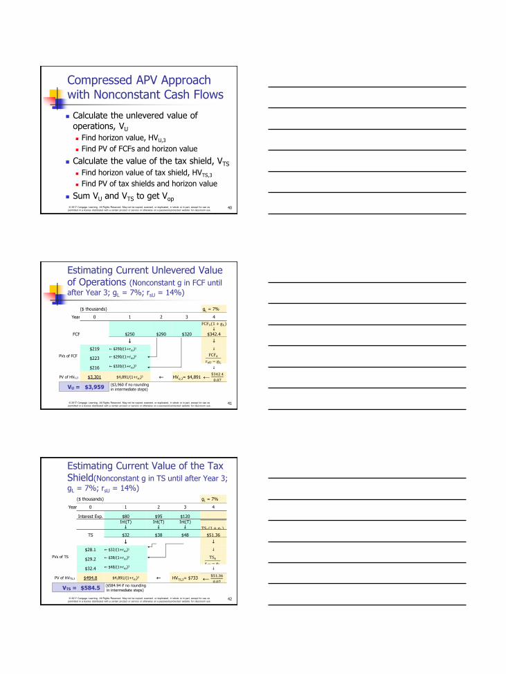
Compressed APV Approach with Nonconstant Cash Flows

Calculate the unlevered value of

operations, VU

Find horizon value, HVU,3

Find PV of FCFs and horizon value

Calculate the value of the tax shield, VTS

Find horizon value of tax shield, HVTS,3

Find PV of tax shields and horizon value

Sum VU and VTS to get Vop

40



Estimating Current Unlevered Value of Operations (Nonconstant g in FCF until

after Year 3; gL = 7%; rsU = 14%)

($ thousands) gL = 7%

Year 0 1 2 3 4

FCF $250 $290 $320

FCF3(1 + gL) ↓

$342.4

↓ ↓

$219 ← $250/(1+rsU)1 ↓

PVs of FCF

$223 ← $290/(1+rsU)2

FCF4rsU − gL

$216 ← $320/(1+rsU)3

↓

PV of HVU,3 $3,301 $4,891/(1+rsU)3 ← HVU,3= $4,891 ←

$342.4

0.07

VU = $3,959 ($3,960 if no rounding in intermediate steps)

41



Estimating Current Value of the Tax Shield(Nonconstant g in TS until after Year 3;

gL = 7%; rsU = 14%)

($ thousands) gL = 7%

Year 0 1 2 3 4

Interest Exp. $80 $95 $120 Int(T) ↓

Int(T) ↓

Int(T) ↓

TS $32 $38 $48 $51.36

↓ ↓

$28.1 ← $32/(1+rsU)1 ↓

PVs of TS

$29.2 ← $38/(1+rsU)2

$32.4 ← $48/(1+rsU)3

↓

PV of HVTS,3 $494.8 $4,891/(1+rsU)3 ← HVTS,3= $733

VTS = $584.5 ($584.94 if no rounding in intermediate steps)

42



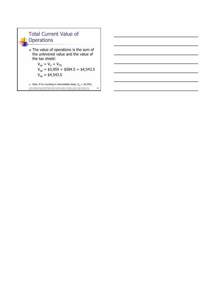
Total Current Value of Operations

The value of operations is the sum of the unlevered value and the value of the tax shield:

Vop = VU + VTS

Vop = $3,959 + $584.5 = $4,543.5

Vop = $4,543.5

Note: If no rounding in intermediate steps, Vop = $4,445).

43

capital structure advanced issues - wz.uw.edu.pl · net operating profit after taxes ... financial...

Documents