Finance and Economics Discussion SeriesDivisions of Research & Statistics and Monetary Affairs

Federal Reserve Board, Washington, D.C.

Capital Misallocation and Secular Stagnation

Caggese and Perez-Orive (2017)

2017-009

Please cite this paper as:Caggese, Andrea and Ander Perez-Orive (2017). “Capital Misallocation and Secular Stagna-tion,” Finance and Economics Discussion Series 2017-009. Washington: Board of Governorsof the Federal Reserve System, https://doi.org/10.17016/FEDS.2017.009.

NOTE: Staff working papers in the Finance and Economics Discussion Series (FEDS) are preliminarymaterials circulated to stimulate discussion and critical comment. The analysis and conclusions set forthare those of the authors and do not indicate concurrence by other members of the research staff or theBoard of Governors. References in publications to the Finance and Economics Discussion Series (other thanacknowledgement) should be cleared with the author(s) to protect the tentative character of these papers.

Capital Misallocation and Secular Stagnation*

Andrea Caggese Ander Pérez-OriveUniversitat Pompeu Fabra, Federal Reserve Board

CREI, & Barcelona GSE

(This Version: January 17, 2017)

Abstract

The widespread emergence of intangible technologies in recent decades may have signifi-

cantly hurt output growth—even when these technologies replaced considerably less productive

tangible technologies—because of structurally low interest rates caused by demographic forces.

This insight is obtained in a model in which intangible capital cannot attract external finance,

firms are credit constrained, and there is substantial dispersion in productivity. In a tangibles-

intense economy with highly leveraged firms, low rates enable more borrowing and faster debt

repayment, reduce misallocation, and increase aggregate output. An increase in the share of

intangible capital in production reduces the borrowing capacity and increases the cash hold-

ings of the corporate sector, which switches from being a net borrower to a net saver. In this

intangibles-intense economy, the ability of firms to purchase intangible capital using retained

earnings is impaired by low interest rates, because low rates increase the price of capital and

slow down the accumulation of corporate savings.

Keywords: Intangible Capital, Borrowing Constraints, Capital Reallocation, Secular StagnationJEL Classification: E22, E43, E44

* A previous version of this paper was entitled "Reallocation of Intangible Capital and Secular Stagnation".We thank Andrew Abel, Fiorella de Fiore (discussant), Wouter Den Haan (discussant), Andrea Eisfeldt, An-tonio Falato, Maryam Farboodi (discussant), Simon Gilchrist, Adam Guren, Matteo Iacoviello, Arvind Krish-namurthy, Tim Landvoigt (discussant), Claudio Michelacci (discussant), Guillermo Ordonez, Enrico Perotti,Vincenzo Quadrini, and Stephen Terry, and seminar participants at Boston University, Boston College, the Fed-eral Reserve Board, the Bank of Spain, the CREI macro lunch, the 7th Meeting of the Macro Finance Society(UCLA 2016), the 2016 Barcelona Summer Forum Workshop on Financial Markets and Asset Prices, the 2016NBER SI Workshop on Macro, Money and Financial Frictions, the Midwest Macro Meetings, the Cleveland FedDay-Ahead Meeting on Productivity, the BoE Workshop on Finance, Investment and Productivity, and the Bankof Italy Workshop on Macroeconomic Dynamics for very helpful comments. We also thank Christoph Albert forexcellent research assistance. Andrea Caggese acknowledges financial support from the Ministry of Economics ofSpain and from Resercaixa. The views expressed in this paper are solely the responsibility of the authors andshould not be interpreted as reflecting the views of the Board of Governors of the Federal Reserve System or ofanyone else associated with the Federal Reserve System. All errors are, of course, our own responsibility.

1 Introduction

Real interest rates have decreased in past decades, while economic growth has fallen short

of previous trends, developments that have been linked to a process of ’secular stagnation’

(Summers (2015), Eichengreen (2015)). At the same time, the developed world has experienced a

technological change toward a stronger importance of information technology and of knowledge,

human and organizational capital, which has gradually reduced the reliance on physical capital

(Corrado and Hulten (2010a)) and has been linked to a significant decrease in corporate net

borrowing (Falato, Kadyrzhanova, and Sim (2014), Döttling and Perotti (2015)).1

This paper argues that the increased reliance on intangible capital and the low real interest

rates interact to hurt capital reallocation and reduce productivity and output growth. Aggregate

productivity depends on an effi cient reallocation of resources from declining or exiting firms to

new entrants or expanding firms. The rise of intangible capital implies a growing importance of

the reallocation of intangible assets such as patents, brand equity, and human and organizational

capital. These assets cannot be collateralized, and their acquisition has to be financed mostly

using retained earnings. As a result, the corporate sector borrows less, holds an increasing

amount of cash, and switches from being a net borrower to a net saver. A decrease in interest

rates increases the price of these intangible assets and reduces the ability of credit-constrained

expanding firms to purchase them. Lower interest rates also decrease the rate at which non-

investing firms can accumulate savings to finance future expansions. We show that the rise in

intangibles, via these effects, alters the dynamic relationship between interest rates and effi ciency

in the allocation of capital.

We formalize this intuition by developing a model of an economy in which firms use tangible

capital, intangible capital, and labor as complementary factors in the production of consumption

goods. A subset of firms have high productivity and suffer from financing constraints that

prevent them from issuing equity or from borrowing any amount in excess of the collateral

value of their holdings of tangible and intangible capital. We follow Kiyotaki and Moore (2012)

in assuming that these high-productivity firms can invest only occasionally. In equilibrium,

they save as much as possible in non-investing periods, and invest all of their accumulated net

savings plus their maximum available borrowing in investing periods. Any residual capital not

absorbed by the high-productivity firms is used by low-productivity firms, which are financially

unconstrained.1The decrease in corporate net borrowing has translated into a shift in the net financial position of the

nonfinancial corporate sector from a net borrowing position roughly before the year 2000 to a net saving positionfrom 2000 onward (Armenter and Hnatkovska (2016), Quadrini (2016), Chen, Karabarbounis, and Neiman (2016),Shourideh and Zetlin-Jones (2016)).

2

In our economy, the consumer sector is modeled as overlapping generations of households

displaying a realistic life cycle, in a way that enables us to obtain an equilibrium interest rate

in the steady state that is not necessarily equal to the household rate of time preference. This

specification of the consumer sector allows us to consider some of the main structural forces

that multiple studies have identified to have pushed real interest rates lower in recent decades.

In particular, we focus on a higher propensity to save in the household sector due to an increase

in household longevity and a decrease in the rate of time preference.2 The increased corporate

net savings due to a higher intangibles usage also contributes to the downward pressure on real

rates.

We first inspect the analytical solution of a simplified version of the model to describe four

channels through which lower interest rates interact with the intensity of intangible capital

in firms’production function to affect the steady state equilibrium of our economy. First, a

debt overhang channel allows net borrowing high-productivity firms to pay down their debt

more easily when interest rates are low and enables them to absorb more capital. Second,

and conversely, a savings channel operates when the firm sector is a net saver: reductions in

the interest rate decrease the speed of accumulation of savings and hurt capital reallocation.

Third, lower interest rates that increase the price of tangible and intangible assets reduce the

amount of capital that high-productivity firms can purchase for a given amount of net worth and

borrowing capacity—a capital purchase price channel. Fourth, a lower interest rate increases the

present value of the collateral pledged next period, and reduces the size of the downpayment

necessary to purchase capital, improving capital reallocation through a borrowing/collateral

value channel. The analytical solution of the simplified model provides a clear illustration of

the main theoretical finding of the paper: in an economy with a relatively low collateral value of

capital, the savings and the capital purchase price channels dominate and a drop in the interest

rate worsens the allocation of resources and reduces aggregate investment, productivity, and

output.

In the remaining sections of the paper, we calibrate and simulate our full general equilibrium

model to study how the parallel developments in the household and corporate sectors have

interacted to generate aggregate patterns consistent with the secular stagnation hypothesis. In

the household sector, as discussed earlier, we model a progressive decrease in individuals’rate of

time preference and a progressive increase in their life expectancy, both of which put downward

pressure on the equilibrium interest rate. In the corporate sector, we introduce a gradual shift

2We interpret our exercise as a shortcut for a collection of different factors, such as population aging, wealthand income inequality, financial deepening, and foreign-sector developments, which have contributed to increasehouseholds’demand for savings in the past 40 years.

3

in the reliance on intangible capital of firms.3

We find that while the household sector developments in isolation and the corporate sec-

tor developments in isolation are both expansionary, the combination of both developments is

contractionary. The drop in the interest rate increases high-productivity firms’ability to bor-

row and pay down their debt while firms still rely strongly on tangible capital. As firms use

increasingly more intangible capital and become net savers, low rates reduce effi cient capital

allocation by increasing capital prices and by slowing the accumulation of corporate savings.

The share of output produced by the high-productivity firms drops significantly. The lower

corporate borrowing itself also puts downward pressure on interest rates, which amplifies the

misallocation of capital. Despite the fact that the economy is shifting toward a higher reliance

on a more productive type of capital, aggregate productivity falls by 6.5%, and even though low

rates encourage capital creation, output is 2% lower than in the case in which only household

sector or only corporate sector developments occur.

We interpret this comparative static exercise as capturing the developments in the U.S.

economy following the rise in the share of intangible capital and the rise in net household and

foreign-sector savings in the past 40 years. In this respect, this model is remarkably consistent

with a series of well-documented trends during this period: (i) net corporate savings increased

as a fraction of gross domestic product (GDP), (ii) household leverage increased as a fraction of

GDP, (iii) the real interest rate fell, (iv) intra-industry dispersion in productivity has increased,

and (v) output and productivity progressively declined relative to their previous trends.

An important question is whether the trends identified in this paper are likely to persist,

as in the secular stagnation hypothesis, or reverse. While the technological shift identified in

the paper is likely to be permanent and possibly intensify, the developments that are keeping

interest rates low may fade in the future. Some developments pushing down rates, such as the

lower retirement age or the increase in the net demand for safe assets, may prove temporary,

while others, such as population ageing, the decline in the growth rate of population, or the

drop in the relative price of capital, might be more persistent.4

Overall, our results suggest that the interaction between low interest rates, intangible tech-

nologies, and corporate financing patterns might be an important factor behind secular stagna-

tion.3We set the reliance on intangible capital to match its observed evolution from a pre-1980 value of 20%

of aggregate capital to a post-2010 value of 60% of aggregate capital (Corrado and Hulten (2010a), Falato,Kadyrzhanova, and Sim (2014), Döttling and Perotti (2015)). Since we assume that intangible capital is moreproductive than tangible capital, this gradual shift is consistent with the notion of the transition to intangiblecapital as a privately optimal choice of firms adopting technologies that are more productive.

4For a detailed discussion of the causes of low real interest rates and the likelihood that these causes remainin the future, see Baldwin and Teulings (2014), Summers (2014), and Blanchard, Furceri and Pescatori (2014).

4

Related Literature

The secular stagnation hypothesis as an explanation of recent economic trends has been

proposed by, among others, Summers (2015) and Eichengreen (2015). One prominent example

of a formalization of these ideas is Eggertsson and Mehrotra (2014), who show how a persistent

tightening of the debt limit facing households can reduce the equilibrium real interest rate and,

in the presence of sticky prices and a zero lower bound in nominal interest rates, generate

permanent reductions in output.5 Our paper contributes to this literature by identifying and

formalizing a novel misallocation effect of endogenously low real interest rates. Our alternative

explanation of the secular stagnation hypothesis can account for a large drop in aggregate

output, does not rely on the zero lower bound or sticky prices, and is consistent with a broad

set of well-documented trends.

The rising use of intangible capital has been documented by Corrado and Hulten (2010a),

and its relation to the decrease in corporate borrowing and the rise in corporate cash holdings

has been shown empirically by Bates, Kahle, and Stulz (2009). Giglio and Severo (2012),

Falato, Kadyrzhanova, and Sim (2014) and Döttling and Perotti (2015) introduce models that

describe how the rise in intangibles can lower the equilibrium interest rate by decreasing firms’

net borrowing. We add to this literature by describing a mechanism through which the rise in

intangibles can have a negative effect on aggregate capital reallocation and growth.

Our paper is also related to the literature on financial frictions, firm dynamics, and misal-

location (Buera, Kaboski, and Shin (2011), Caggese and Cuñat (2013), Moll (2014), Midrigan

and Xu (2014), and Buera and Moll (2015)). With respect to these papers, our contribution is

to provide novel theoretical insights on the relation between interest rates, the collateralizability

of capital, and misallocation.6

The rest of the paper is organized as follows. Section 2 introduces the empirical evidence

that motivates this paper. We describe a very simple model in Section 3 that conveys the basic

intuition of the mechanisms we introduce, and we develop a full-fledged general equilibrium

extension in Section 4. The steady state and calibration of the general equilibrium model are

described in Section 5 and the simulation results are discussed in Section 7. Section 8 concludes.5Other recent theoretical papers with alternative explanations of secular stagnation are Bacchetta, Benhima,

and Kalantzis (2016) and Benigno and Fornaro (2015).6Gopinath et al. (2016) also consider a model with financial frictions and heterogenous firms in which declining

interest rates cause an increase in the dispersion in the productivity of capital. However, their mechanism isfundamentallty different from ours. In their model, when the interest rate falls, all firms invest more and expandaggregate capital and ouput. Productivity dispersion increases because larger firms are able to grow more rapidlythan smaller and more financially constrained ones. In our model, instead, low rates tighten financial constraintsof high-productivity firms that utilize intangible capital, and reduce their investment.

5

2 Empirical Motivation

In this section, we summarize the key stylized facts that motivate our model.

1 - Developed economies are significantly more reliant on intangible capital now

than in the 1980s, and this technological shift has been linked to the simultaneous

transition of the corporate sector from net debtor to net saver.

The developed world has experienced a technological change toward a stronger importance

of information technology and of knowledge, human, and organizational capital, which has

gradually reduced the reliance on physical capital (Brown, Fazzari and Petersen (2009), Corrado

and Hulten (2010a), Falato, Kadyrzhanova, and Sim (2014)). In the United States, intangible

capital as a share of total capital went from around 0.2 in the 1970s to 0.5 in the 2000s (Falato,

Kadyrzhanova, and Sim (2014)). In parallel, there has been a shift in the net financial position

of the nonfinancial corporate sector from a net borrowing position roughly before the year 2000

to a net saving position from 2000 onward (Armenter and Hnatkovska (2016), Quadrini (2016),

Chen, Karabarbounis, and Neiman (2016), Zetlin-Jones and Shourideh (2016)).

The empirical evidence suggests that these two trends are related. The process of techno-

logical change has been linked to a lower availability of collateral for the corporate sector, which

has lowered its debt capacity. Brown, Fazzari, and Petersen (2009) document that U.S. firms

finance most of their research and development (R&D) expenditures out of retained earnings

and equity issues, an observation in line with the conclusion in Hall (2002) that R&D-intensive

firms feature much lower leverage, on average, than less R&D-intensive firms. Gatchev, Spindt,

and Tarhan (2009) document that, in addition to R&D, marketing expenses and product devel-

opment are also mostly financed out of retained earnings and equity. In contrast, tangible assets

are mostly financed with debt.7 The process of technological change has also been linked to an

increase in the precautionary motives for cash accumulation to avoid future financial shortages

(Bates, Kahle, and Stulz (2009), Falato, Kadyrzhanova, and Sim (2014), Falato and Sim (2014),

Döttling and Perotti (2015), Begenau and Palazzo (2016)).8

Furthermore, firm-level empirical evidence suggests that the observed link between intangible

intensity and high cash holdings is driven by financial frictions. Begenau and Palazzo (2016)

7Eisfeldt and Rampini (2009) report that a big share of machinery, equipment, buildings and other structuresis financed with debt. Inventory investment and other tangible short-term assets attract substantial debt financein the form of trade credit and bank credit lines (Petersen and Rajan (1997), Sufi (2009)). Finally, investment incommercial real estate is primarily financed with mortgage loans (Benmelech, Garmaise, and Moskowitz (2005)).

8Lack of access to debt financing of firms that rely on intangible capital could be compensated by easy accessto equity financing. While easy access to equity financing would be consistent with the observed lower leverage ofthese firms, it would be harder to reconcile with the remarkable accumulation of cash holdings. A large body ofevidence shows that external equity financing is significantly costly (Altinkilic and Hansen (2000), Gomes (2001),Belo, Lin and Yang (2016)).

6

introduce evidence showing that an important determinant of the increase in cash holdings

of public firms is the increase in frequency of new firms that are very R&D intensive, and

they suggest that these trends are consistent with a model in which cash holdings are driven

by financial frictions of the R&D-intensive firms and costly equity financing. Similarly, Falato,

Kadyrzhanova, and Sim (2014) show empirically that the relation between reliance on intangible

capital and cash holdings is stronger among firms for which financing frictions are more severe.

2 - Productivity dispersion has increased in intangibles sectors during recent

decades, while it has remained roughly constant in tangibles sectors.

Kehrig (2015) analyzes establishment-level manufacturing data from the U.S. census and

documents a significant increasing trend in the dispersion of productivity across firms within

sectors over the past 40 years. Earlier, we provided evidence that the rising intangible capital

share is related to an increase in firm-level cash holdings to overcome external finance con-

straints. If the misallocation of resources caused by financial constraints is a factor contributing

to the increase in productivity dispersion, we should expect the latter to be more pronounced

in sectors with higher intensity of intangible capital.9 In order to investigate the relation be-

tween the rise in intangibles and productivity dispersion, we use accounting data of 34,900 U.S.

corporations obtained from Compustat, covering the period from 1980 to 2015, and containing

379,318 firm-year observations. We define intangible capital as the sum of knowledge capital and

organizational capital. We consider two alternative productivity measures: labor productivity

(y) and total factor productivity (TFP) (A) (see Appendix A for details). Our measure of mis-

allocation, the productivity dispersion, is computed as the standard deviation of the difference

between the logs of the productivity of firm i and the aggregate productivity of the industry s

in which firm i operates.

[FIGURE 1 ABOUT HERE]

[FIGURE 2 ABOUT HERE]

Figures 1 and 2 plot the dispersion of labor productivity and TFP, respectively, in 2-digit

SIC industries over time (normalized by the value in 1980). In both figures, the left graph shows

average dispersion for all sectors, and it replicates the upward-sloping trend already documented

9 It is important to note that this paper, like Kehrig (2015), analyzes the dynamics of the cross-sectionaldispersion of productivity, not the dispersion of business growth rates. Davis et al. (2006) focus on the latter,and using both firm- and establishment-level data document a negative trend instead. These opposite trendsare consistent with the findings of our model, in which a decline in the growth rate of expanding firms reducesreallocation of capital and increases steady state productivity differences.

7

by Kehrig (2015) using establishment-level data. In the right graph, the red dashed line shows

the mean of the dispersion measure across industries (weighted by sales) in the top 50%, and

the blue line in the bottom 50%, of the distribution of the industry-wide ratio of intangible

capital to total capital (averaged across years).10 Both figures show that the constant rise

in the within-industry dispersion of productivity is driven by the sectors with higher average

shares of intangible capital. This evidence is consistent with the hypothesis that intangible

capital exacerbates misallocation problems caused by financial frictions. Appendix A discusses

two additional exercises that provide robustness to these results.

3 Simple and Intuitive Explanation of the Mechanisms

We introduce in this section the simplest possible model that can describe our proposed mecha-

nisms and deliver analytical results. Our main interest is studying how exogenous interest rate

variations affect the allocation of capital and aggregate output depending on the degree of tan-

gibility of capital. This framework is extended in Section 4 in a full-fledged general equilibrium

setup that can be used for realistic quantitative analysis.

Consider an infinite-horizon, discrete-time model of the final goods producers of an econ-

omy. Firms use capital, which is in constant aggregate supply K, to produce a homogeneous

consumption good using a constant-returns-to-scale technology. There are two types of firms,

high-productivity and low-productivity. Effi ciency is determined by the share of K allocated to

high-productivity firms. Here we present the aggregate steady state equilibrium conditions and

introduce the details of the derivation of this simple model in Appendix B.

Aggregate output in the steady state is

Y = Y p + Y u + Y e = zK + zu(K −K

), (1)

where z captures the productivity of high-productivity firms and zu < z captures the produc-

tivity of low-productivity firms.

Aggregate capital holdings K of the high-productivity firms, which are assumed to be finan-

10The sectors with high shares of intangible capital are: Chemicals and Allied Products; Industrial and Com-mercial Machinery and Computer Equipment; Electronic & Other Electrical Equipment & Components; Trans-portation Equipment; Measuring, Photographic, Medical, & Optical Goods, & Clocks; Miscellaneous Manu-facturing Industries; Wholesale Trade - Durable Goods; Home Furniture, Furnishings and Equipment Stores;Miscellaneous Retail Business Services; and Engineering, Accounting, Research, and Management Services.The sectors with low shares of intangible capital are: Oil and Gas Extraction; Food and Kindred Prod-

ucts; Paper and Allied Products; Rubber and Miscellaneous Plastic Products; Stone, Clay, Glass, and ConcreteProducts; Primary Metal Industries; Fabricated Metal Products; Wholesale Trade - Nondurable Goods; GeneralMerchandise Stores; Food Stores; Apparel and Accessory Stores; and Eating and Drinking Places.

8

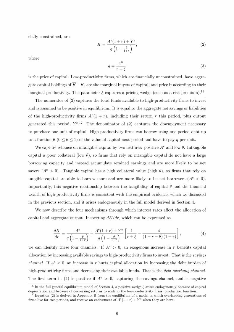
cially constrained, are

K =Ae(1 + r) + Y e

q(

1− θ1+r

) , (2)

where

q =zu

r + ξ(3)

is the price of capital. Low-productivity firms, which are financially unconstrained, have aggre-

gate capital holdings of K−K, are the marginal buyers of capital, and price it according to their

marginal productivity. The parameter ξ captures a pricing wedge (such as a risk premium).11

The numerator of (2) captures the total funds available to high-productivity firms to invest

and is assumed to be positive in equilibrium. It is equal to the aggregate net savings or liabilities

of the high-productivity firms Ae(1 + r), including their return r this period, plus output

generated this period, Y e.12 The denominator of (2) captures the downpayment necessary

to purchase one unit of capital. High-productivity firms can borrow using one-period debt up

to a fraction θ (0 ≤ θ ≤ 1) of the value of capital next period and have to pay q per unit.

We capture reliance on intangible capital by two features: positive Ae and low θ. Intangible

capital is poor collateral (low θ), so firms that rely on intangible capital do not have a large

borrowing capacity and instead accumulate retained earnings and are more likely to be net

savers (Ae > 0). Tangible capital has a high collateral value (high θ), so firms that rely on

tangible capital are able to borrow more and are more likely to be net borrowers (Ae < 0).

Importantly, this negative relationship between the tangibility of capital θ and the financial

wealth of high-productivity firms is consistent with the empirical evidence, which we discussed

in the previous section, and it arises endogenously in the full model derived in Section 4.

We now describe the four mechanisms through which interest rates affect the allocation of

capital and aggregate output. Inspecting dK/dr, which can be expressed as

dK

dr=

Ae

q(

1− θ1+r

) +Ae(1 + r) + Y e

q(

1− θ1+r

) [1

r + ξ− θ

(1 + r − θ) (1 + r)

], (4)

we can identify these four channels. If Ae > 0, an exogenous increase in r benefits capital

allocation by increasing available savings to high-productivity firms to invest. That is the savings

channel. If Ae < 0, an increase in r hurts capital allocation by increasing the debt burden of

high-productivity firms and decreasing their available funds. That is the debt overhang channel.

The first term in (4) is positive if Ae > 0, capturing the savings channel, and is negative

11 In the full general equilibrium model of Section 4, a positive wedge ξ arises endogenously because of capitaldepreciation and because of decreasing returns to scale in the low-productivity firms’production function.12Equation (2) is derived in Appendix B from the equilibrium of a model in which overlapping generations of

firms live for two periods, and receive an endowment of Ae(1 + r) + Y e when they are born.

9

if Ae < 0, capturing the debt overhang channel. The capital purchase price channel is the

mechanism through which increases in r benefit capital reallocation by decreasing q and making

capital cheaper. The first term inside the square brackets in (4) captures this channel and is

always positive. Finally, the collateral value channel is the channel through which increases

in r hurt capital reallocation by decreasing the value of firms’collateral (the term θ/ (1 + r))

and tightening the borrowing constraint. The second term inside the brackets represents this

channel and is always negative.

How do these four channels depend on the intensity of intangible capital? In other words,

how does the tangibility of capital matter for the effect of variations in r on the effi ciency of

this economy? For clarity of exposition, assume that a tangibles-intensive economy is one in

which Ae < 0 and θ > 0, and that an intangibles-intensive economy is one in which Ae > 0 and

θ = 0. Then

sign

[dK

dr(tangib le)

]=

Ae

q(

1− θ1+r

)<0

+Ae(1 + r) + Y e

q(

1− θ1+r

) 1

r + ξ>0

− θ

(1 + r − θ) (1 + r)<0

< 0 if (5) is met,

and

sign

[dK

dr(intangib le)

]=Ae

q>0

+Ae(1 + r) + Y e

q

1

r + ξ>0

> 0 always.

The derivative dKdr is positive in an intangibles economy, meaning that a reduction in r is

unambiguously contractionary. It is instead most likely expansionary in a tangibles economy,

particularly if the responsiveness of q to r is limited (ξ is high) and the borrowing capacity is

large (θ is high). More specifically, a decrease in r is unambiguously expansionary in a tangibles

economy if the following condition is satisfied:

θ >1 + 2r + r2

1 + 2r + ξ. (5)

Taken together, these results suggest that the degree of tangibility of capital in an economy

matters importantly for how exogenous variations in the interest rate affect capital allocation

and output and describe four important channels through which these effects occur. Crucially,

they show that falling interest rates can become contractionary in an economy that relies on

intangible capital.

Section 4 provides a full-fledged model in which we endogenize firms’financing constraints,

saving and borrowing decisions, and investment, households’consumption and savings, and the

10

interest rate, wages, and the prices of tangible and intangible capital.

The Investment Demand Curve

To provide a deeper understanding of how the features of the equilibrium of this economy

change as a result of a transition from an economy reliant on tangible capital to one in which

intangible capital acquires a larger importance, we represent the equilibrium in the credit market

in Figure 3. The main objective is to provide an empirically relevant assessment of the slope of

the investment demand curve for different values of θ. To do so, we calibrate the parameters

at the annual frequency to be broadly consistent with observed moments of U.S. data. We

postpone a more thorough calibration to the full model developed in Section 4. We study

a range of the real interest rate between r = 6% and r = 0%, consistent with the observed

evolution of real rates between the early 1980s and the present. We normalize the productivity

of low-productivity firms to zu = 1 and the output endowment to Y e = 1. We consider a

tangibles economy to feature a pledgeability parameter of capital θ equal to 0.9 and a net

borrowing position equivalent to 20% of output (Ae = −0.2). We consider an intangibles

economy to feature a pledgeability parameter of capital θ equal to 0.4 and a net saving position

equivalent to 20% of output (Ae = 0.2). The interest rate wedge ξ is set at 20% and is meant to

capture a combination of factors such as risk premia, default premia, and capital depreciation.

[FIGURE 3 ABOUT HERE]

In Figure 3, the upward-sloping savings curve captures the combination of the (unmodeled)

net savings of the household sector. Higher interest rates induce households to save more,

under the empirically realistic assumption that the substitution effect dominates the income

effect for them. The demand for capital by investing firms is equal to the amount borrowed

by them plus (minus) the savings (debt) they carry over from the previous period. This curve

can be upward or downward sloping depending on the relevance of intangible capital in the

production function. In an economy where capital is interpreted to be of a tangible nature

(θ = 0.9 and Ae = −0.2), an increase in aggregate savings has the effect of lowering interest

rates and increasing capital purchases from expanding firms. When there is a shift outward in

the savings curve, the economy moves from point A to point B. The collateral value channel

and the debt overhang channel dominate. As a result, a larger share of the capital stock is in

the hands of high-productivity firms, which improves the allocation of resources and increases

aggregate productivity and output. Instead, in an economy where capital is interpreted to be of

an intangible nature (θ = 0.4 and Ae = 0.2), the demand for capital curve is upward sloping due

to the strength of the capital price and savings channels. As interest rates rise, firms demand

11

more capital because they have larger savings and the price of capital is lower. In this case, an

outward shift in the savings schedule generates a decrease in the equilibrium capital purchases

of high-productivity firms, because the decrease in interest rates the shift in savings generates

hurts the reallocation of capital toward high-productivity firms. The economy moves from point

A to point C, worsening the allocation of resources and reducing aggregate productivity and

output.

4 General Equilibrium Model

We introduce an infinite-horizon, discrete-time economy populated by an intermediate sector

that produces capital; by a final good sector in which firms use labor and capital to produce

consumption goods; and by households, which provide labor and own both sectors. There are

several important extensions to the simple model analyzed in Section 3, and we describe the main

ones here. We introduce an intermediate capital producing sector that allows us to endogenize

in equilibrium the aggregate stock of capital. In the final good sector, we model explicitly

tangible and intangible capital, and we derive endogenously the accumulation of financial and

physical assets of firms that live multiple periods. The household sector is modeled as a life-

cycle framework, which allows us to endogenize the interest rate and study how it is affected

by demographic changes and other demand-side factors.

4.1 The Capital-Producing Sector

A representative firm in this sector chooses investment in tangible and intangible capital, re-

spectively ITt and IIt , in order to maximize profits:

maxIJ

qJ,tIJt − bJt

(IJtϕ

)ϕ, (6)

where ϕ > 1, bJt > 0, and qJ,t is the price of the type of capital J ∈ {T, I}. We allow for bTt and

bIt to be time varying in order to capture trends in the evolution of the relative price of capital.

The first order condition yields IJt = ϕ(qJ,tbJt

) 1ϕ−1

, and profits are πJt =q

ϕϕ−1J,t

bJ 1ϕ−1

t

(ϕ− 1) .

At the beginning of period t, total capital available is KTt and K

It . New capital I

Tt and I

It is

produced and sold in period t so that the aggregate dividends generated by the capital-producing

sectors are

Dkt = πTt + πIt . (7)

During period t, tangible capital and intangible capital depreciate at the rates 0 ≤ δ < 1.

12

And the law of motion of aggregate capital is

KJt+1 = IJt + (1− δ)KJ

t ,

with J ∈ {T, I} .

4.2 Final Good Sector

There are two types of final-good-producing firms: high-productivity and low-productivity.

4.2.1 The High-Productivity Firms

There is a continuum of mass 1 of high-productivity firms.

Technology and financing opportunities

High-productivity firms produce a final good using a constant-returns-to-scale production

function that is Cobb-Douglas in labor and capital. The firms use two different types of com-

plementary capital, tangible and intangible. For simplicity, we assume that they are perfect

complements. The production function takes the following form:

ypt = zt (µ)n(1−α)t

[min

(kT,t

1− µ,kI,tµ

)]α, (8)

where 0 < α ≤ 1 and 0 < µ < 1. The terms kT,t and kI,t represent tangible and intangible

capital installed in period t− 1 that produce output in period t, and nt is labor. The Leontief

production structure implies that, in equilibrium, intangible capital as a share of total capital

in high-productivity firms is equal to µ. The productivity term zt (µ) is increasing in the share

of intangible capital and captures the higher productivity of more intangibles-intensive tech-

nologies. We drop from now on reference to the dependence of zt on µ for ease of notation and

defer discussion of their relationship to the calibration section.

The budget constraint for high-productivity firms is given by the following dividend equation:

dt = ypt + (1 + rt)af,t− af,t+1− qT,t (kT,t+1 − (1− δ)kT,t)− qI,t(kI,t+1− (1− δ)kI,t)−wtnt, (9)

where rt is the interest rate paid or received in date t; qT,t, and qI,t are the prices of tangible

and intangible capital, respectively; and wt is the wage. The term af,t > 0 indicates that the

firm is a net saver, and af,t < 0 indicates that the firm is a net borrower.

High-productivity firms are subject to frictions in their access to external finance. They are

13

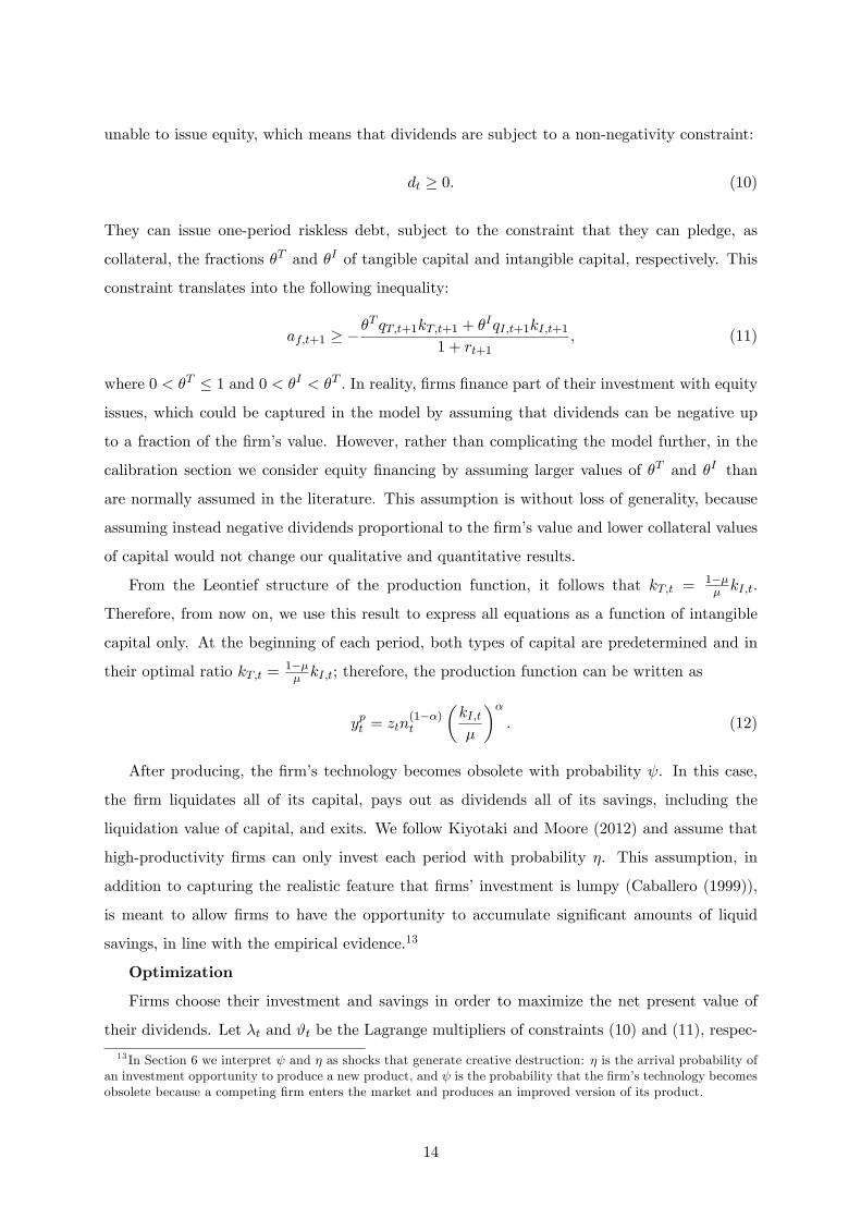
unable to issue equity, which means that dividends are subject to a non-negativity constraint:

dt ≥ 0. (10)

They can issue one-period riskless debt, subject to the constraint that they can pledge, as

collateral, the fractions θT and θI of tangible capital and intangible capital, respectively. This

constraint translates into the following inequality:

af,t+1 ≥ −θT qT,t+1kT,t+1 + θIqI,t+1kI,t+1

1 + rt+1, (11)

where 0 < θT ≤ 1 and 0 < θI < θT . In reality, firms finance part of their investment with equity

issues, which could be captured in the model by assuming that dividends can be negative up

to a fraction of the firm’s value. However, rather than complicating the model further, in the

calibration section we consider equity financing by assuming larger values of θT and θI than

are normally assumed in the literature. This assumption is without loss of generality, because

assuming instead negative dividends proportional to the firm’s value and lower collateral values

of capital would not change our qualitative and quantitative results.

From the Leontief structure of the production function, it follows that kT,t = 1−µµ kI,t.

Therefore, from now on, we use this result to express all equations as a function of intangible

capital only. At the beginning of each period, both types of capital are predetermined and in

their optimal ratio kT,t = 1−µµ kI,t; therefore, the production function can be written as

ypt = ztn(1−α)t

(kI,tµ

)α. (12)

After producing, the firm’s technology becomes obsolete with probability ψ. In this case,

the firm liquidates all of its capital, pays out as dividends all of its savings, including the

liquidation value of capital, and exits. We follow Kiyotaki and Moore (2012) and assume that

high-productivity firms can only invest each period with probability η. This assumption, in

addition to capturing the realistic feature that firms’investment is lumpy (Caballero (1999)),

is meant to allow firms to have the opportunity to accumulate significant amounts of liquid

savings, in line with the empirical evidence.13

Optimization

Firms choose their investment and savings in order to maximize the net present value of

their dividends. Let λt and ϑt be the Lagrange multipliers of constraints (10) and (11), respec-

13 In Section 6 we interpret ψ and η as shocks that generate creative destruction: η is the arrival probability ofan investment opportunity to produce a new product, and ψ is the probability that the firm’s technology becomesobsolete because a competing firm enters the market and produces an improved version of its product.

14

tively. We define the value function conditional on having an investment opportunity, denoted

V +(kI,t, af,t), as follows:

V +t (kI,t, af,t) = max

nt,dt,af,t+1,kI,t+1(1 + λt)dt + ϑt

(af,t+1 +

θT qT,t+1kT,t+1 + θIqI,t+1kI,t+1

1 + rt+1

)+

1

1 + rt+1

[(1− ψ)Vt+1(kI,t+1, af,t+1) + ψdexitt+1

], (13)

where

dexitt = ypt + (1 + rt)af,t + (1− δ)qT,t1− µµ

kI,t + (1− δ)qI,tkI,t − wt, (14)

and Vt+1(kI,t+1, af,t+1) is the value function conditional on continuation but before the invest-

ment shock is realized:

Vt+1(kI,t+1, af,t+1) = ηV +(kI,t+1, af,t+1) + (1− η)V −(kI,t+1, af,t+1). (15)

The value function of a non-investing firm, denoted V −(kI,t, af,t), is identical to V +(kI,t, af,t)

but does not offer the opportunity to choose kI,t+1.

The firm solves (13) (or its non-investing counterpart) subject to (9), (10), and (11). We

next provide a characterization of high-productivity firms’optimal choice under the assumption

that they are permanently financially constrained. We claim − and check later in our calibrated

simulations − that, in equilibrium, the marginal return on capital for high-productivity firms

is always higher than their user cost:

∂ypt+1

∂kI,t+1=αzt+1n

(1−α)t+1

µ

(kI,t+1

µ

)α−1

>

(qT,t

1− µµ

+ qI,t

)−

(1− δ)(qT,t+1

1−µµ + qI,t+1

)1 + rt+1

.

(16)

The implication of assumption (16) for investing firms is that the borrowing constraint (11)

is binding, and that firms choose not to pay dividends, so the equity constraint (10) is also

binding. Making dt = 0 in budget constraint (9), using (9) to substitute for af,t+1 in (11),

assuming (11) is binding, and solving for kI,t+1, we obtain their level of investment:

(kI,t+1 | invest) =ypt − wtnt + (1 + rt)af,t + (1− δ)

(qT,t

1−µµ + qI,t

)kI,t

qT,t1−µµ + qI,t −

(θT

qT,t+11+rt+1

1−µµ + θI

qI,t+11+rt+1

) . (17)

The right-hand side of equation (17) is the maximum feasible investment in intangible capital

for a firm. The numerator is the total wealth available to invest. The denominator captures

the downpayment necessary to purchase one unit of kI,t+1 and1−µµ units of kT,t+1. The term

15

qT,t1−µµ + qI,t represents the total cost necessary to purchase these amounts of both types of

capital, and the term θTqT,t+11+rt+1

1−µµ + θI

qI,t+11+rt+1

is the amount that can be financed by borrowing.

Investing firms in equilibrium borrow as much as possible, and

(af,t+1 | invest) = −(θT

qT,t+1

1 + rt+1

1− µµ

+ θIqI,t+1

1 + rt+1

)kI,t+1 < 0. (18)

The implication of assumption (16) for non-investing firms is that they will not sell any of

their capital, and, for these firms, the law of motion of capital is

(kI,t+1 | not invest) = (1− δ)kI,t. (19)

Non-investing firms always retain all earnings and select dt = 0 because they face a positive

probability of being financially constrained in the future, and hence the value of cash inside the

firm is always higher than its opportunity cost (see Appendix C for a formal proof). Substituting

dt = 0 and (19) in (9):

(af,t+1 | not invest) = ypt + (1 + rt)af,t − wtnt. (20)

Equations (18) and (20) determine the wealth dynamics of firms. A firm that invested in pe-

riod t−1 but is not investing in period t has debt equal to−af,t =(θT

qT,t+11+rt+1

1−µµ + θI

qI,t+11+rt+1

)kI,t+1.

It uses current profits ypt −wtnt to pay the interest rate on debt −rtaf,t and to reduce the debt

itself. As long as the firm is not investing, the debt −af,t decreases until the firm becomes a net

saver and has af,t > 0. At this point, wealth accumulation is driven both by profits ypt − wtntand by interest on savings rtaf,t, until the firm has an investment opportunity and its accumu-

lated wealth (1 + rt)af,t is used to purchase capital (see equation (17)). This discussion clarifies

that a lower interest rate rt helps the non-investing firm repay existing debt (the debt hangover

channel), but it slows down the accumulation of savings after the firm has repaid the debt (the

savings channel).

Finally, the first order condition for nt, for both investing and non-investing firms, im-

plies that given the wage wt and its predetermined capital kI,t, a firm will choose the profit-

maximizing level of labor, which determines the optimal capital-labor ratio:

kI,tnt

= µ

[wt

(1− α) zt

] 1α

. (21)

16

4.2.2 The Low-Productivity Firms

There is a mass 1 of identical low-productivity firms that have access to two production func-

tions. Each production function combines capital kuJ,t with specialized labor nuJ,t using a

constant-returns-to-scale technology, where J = {I, T} captures the tangibility of the capital

used. The total amount yut of the homogeneous final good produced is then

yut = zu,It n1−αuI,t k

αuI,t + zu,Tt n1−α

uT,tkαuT,t,

where α determine the capital share. We do not introduce the assumption of perfect complemen-

tarity between tangible and intangible capital (which we do introduce for the high-productivity

firms) to gain tractability in the pricing of capital, as will become clear in the next section. This

is without loss of generality.

This sector is assumed to be able to finance capital with equity from the household sector

and to pay out all profits as dividends dut to households every period:

dut = yut − wuIt nuI,t − wuTt nuT,t − qI,t(kuI,t+1 − (1− δ)kuI,t

)− qT,t

(kuT,t+1 − (1− δ)kuT,t

). (22)

In addition, the low-productivity firms sector is able to remunerate households for their

labor services (wuIt nuI,t + wuTt nuT,t).

The first order conditions for the two types of labor imply that given wages wuIt and wuTt and

a firm’s predetermined capital stocks kuI,t and kuT,t, a low-productivity firm will choose the profit-

maximizing level of each type of labor, which determines the optimal capital-labor ratio:

kuJ,tnuJ,t

=

[wuJt

(1− α) zu,Jt

] 1α

. (23)

Given that low-productivity firms are financially unconstrained, and provided that their

marginal return on each of the two types of capital is lower than for high-productivity firms,

low-productivity firms are willing to absorb all of the capital not demanded by high-productivity

firms, at a price equal to their marginal return on capital.

4.2.3 Aggregation of the Firm Sector and Pricing of Assets

We assume (see Section 4.3) that the aggregate supply of all types of labor is normalized to

N = NuI = NuT = 1. Since all high-productivity firms produce at the optimal capital-labor

ratio determined by equation (21), and the production function is constant returns to scale ,

we can aggregate production across firms to obtain

17

Y pt = zt

(KI,t

µ

)α. (24)

The wage is determined in competitive markets by the marginal return of labor:

wt = (1− α) zt

(KI,t

µ

)α. (25)

And aggregate wealth Wt of the high-productivity firms at the beginning of period t is

Wt ≡ Y pt − wt + (1 + rt)Af,t + (1− δ)

(qT,t

1− µµ

+ qI,t

)KI,t. (26)

Aggregate capital is determined as follows. A fraction (1− ψ) of high-productivity firms

continue activity, and a fraction η of those have an investment opportunity. They have a

fraction (1− ψ) η of total wealth Wt, which they use to buy the amount of capital given by

equation (17). A fraction ψ of high-productivity firms exit, and are replaced by an equal

number of firms with an initial endowment of W0 and no capital. A fraction η of new entrants

invest. Therefore, we define total intangible capital in the hands of investing agents at the end

of period t, expressed in aggregate terms, as ηKINVI,t+1, where K

INVI,t+1 is

KINVI,t+1 =

(1− ψ)Wt + ψW0(qT,t − θT qT,t+1

1+rt+1

)1−µµ + qI,t − θI

qII,t+11+rt+1

. (27)

The (1− η) fraction of surviving firms that do not have an investment opportunity continue

to hold their depreciated capital. Therefore, aggregate capital for the next period is equal to

KI,t+1 = ηKINVI,t+1 + (1− δ) (1− ψ) (1− η)KI,t (28)

and

KT,t+1 =1− µµ

KI,t+1. (29)

Furthermore, we can aggregate the output of low-productivity firms, substituting labor

supply NuI = NuT = 1, and obtain

Y ut = zu,It

(KI −KI,t

)α+ zu,Tt

(KT −KT,t

)α, (30)

wuJt = (1− α) zu,Jt

(KJ −KJ,t

)α, (31)

with J = {I, T}.

The marginal return of capital in the high-productivity firms is as follows. In order obtain

a marginal increase ∂Y pt∂KI,t

= αµzt

(KI,tµ

)α−1, these firms purchase one unit of intangible capital

18

and 1−µµ units of tangible capital. The equilibrium described earlier requires that the high-

productivity firms have the highest return on capital, or

α

µzt

(KI,t+1

µ

)α−1

> zu,It α(KI −KI,t

)α−1+

1− µµ

zu,Tt α(KT −KT,t

)α−1, (32)

where the right-hand side of this inequality captures the marginal return of one unit of tangible

capital and 1−µµ units of intangible capital in the low-productivity firms.

If condition (32) is satisfied, then it follows immediately that the prices of capital are

qI,t = zu,II α(KI −KI,t

)α−1+

1− δ1 + rt+1

qI,t+1, (33)

and

qT,t = zu,Tt α(KT −KT,t

)α−1+

1− δ1 + rt+1

qT,t+1. (34)

If we substitute (33) and (34) into (32), it follows that

α

µzt

(KI,t+1

µ

)α−1

> qI,t −1− δ

1 + rt+1qI,t+1 +

1− µµ

(qT,t −

1− δ1 + rt+1

qT,t+1

), (35)

which implies that the claim (16) is correct. Aggregate financial assets of the high-productivity

firms (Af,t+1) are equal to the assets saved from the previous period by continuing firms,

(1− ψ) ((1 + rt)Af,t), plus their current retained earnings, (1− ψ) (Y pt − wt), plus the endow-

ments of new firms (ψW0)minus total investment,(qT,t

1−µµ + qI,t

)(KI,t+1 − (1− δ) (1− ψ)KI,t):

Af,t+1 = (1− ψ) (Y pt − wt + (1 + rt)Af,t) + ψW0

−(qT,t

1− µµ

+ qI,t

)(KI,t+1 − (1− δ) (1− ψ)KI,t) . (36)

Finally, total dividends paid out by exiting high-productivity firms to households are equal

to

Dpt = ψ

(Y pt − wt + (1 + rt)Af,t +

(qT,t

1− µµ

+ qI,t

)KI,t

)− ψW0, (37)

and the dividends paid by the low-productivity firms are:

Dut = Y u

t −wuIt −wuTt −qI,t[(KI−KI,t+1

)−(KI−KI,t

)]−qT,t

[(KT−KT,t+1

)−(KT−KT,t

)].

4.3 Households

We consider a life-cycle model with two types of households, young and old—with measures Hy

and Ho, respectively—whose sum is normalized to 1. Young households supply three types of

19

differentiated labor: high-productivity firm labor (in exchange for wage wt), low-productivity

intangible technology labor (in exchange for wage wuIt ), and low-productivity tangible technol-

ogy labor (in exchange for wage wuTt ). There is an inelastic aggregate supply of one unit of each

type of labor. Young households receive a fraction γ of the aggregate dividends. Households

remain young for N periods and become old after N+1 periods, so that there is a constant frac-

tion φ = 1N of young households for every age between 1 and N , and, every period, a measure

φHy of households becomes old. Old households cannot work, receive a fraction (1− γ) of ag-

gregate dividends, and die with probability %. The measure of old households Ho is determined

as follows:

Ho = (1− %)Ho + φHy. (38)

At the same time, the measure of young households is

Hy = (1− φ)Hy +Ny, (39)

where Ny is the constant measure of newborn households. From the assumption that Hot +Hy

t =

1, it follows that Ny = φ%φ+% , H

ot = φ

φ+% , and Hyt = %

φ+% .

We follow Blanchard (1985) and Yaari (1965) in assuming that households participate in

a life insurance scheme when old. For the detailed solution of the households’maximization

problem, see Appendix D.

5 Steady State

5.1 Equilibrium

We consider a steady state equilibrium and drop reference to the time subscript t. Total output

of the high-productivity and low-productivity firms is, respectively,

Y p = z

(KI

µ

)α(40)

and

Y u = zu,I(KI −KI

)α+ zu,T

(KT −KT

)α. (41)

Dividends d are given by

d = Dp +Du +Dk, (42)

where

Du = Y u − wuIt − wuT − qIδ(KI −KI

)− qT δ

(KT −KT

),

20

Dp = ψ

(αz

(KI

µ

)α+ (1 + r)Af +

(qT

1− µµ

+ qI

)KI

)− ψW0,

and

Dk =q

ϕϕ−1T,t

bT 1ϕ−1

(ϕ− 1) +q

ϕϕ−1I,t

bI 1ϕ−1

(ϕ− 1) .

Aggregate cash holdings of the high-productivity firms in the steady state can be obtained

by combining (36), (24), and (25) to obtain

Af =(1− ψ)αzt

(KIµ

)α+ ψW0 −

(qT

1−µµ + qI

)[ψ + δ(1− ψ)]KI

[1− (1− ψ) (1 + r)]. (43)

Aggregate borrowing is equal to aggregate savings, or

Af = B, (44)

where B is aggregate household borrowing, which we derive in detail in Appendix D. By Walras’

Law, the aggregate resource constraint is satisfied. In order to determine the aggregate capital

of the high-productivity firms, equation (28) in the steady state is equal to

KI = η(1− ψ)W + ψW0[

qT

(1− θT

1+r

)1−µµ + qI

(1− θI

1+r

)][1− (1− δ)(1− ψ) (1− η)]

, (45)

where W is defined using equation (26) in steady state:

W ≡ αzt(KI

µ

)α+ (1 + r)Af + (1− δ)

(qT

1− µµ

+ qI

)KI . (46)

We can also express (45) as

KI =η(1− ψ)

(αzt

(KIµ

)α+ (1 + r)Af

)+ ηψW0[

qT

(1− θT

1+r

)1−µµ + qI

(1− θI

1+r

)][δ + ψ (1− δ)]−

(qT

θT

1+r1−µµ + qI

θI

1+r

)η(1− δ)(1− ψ)

,

(47)

which has an intuitive explanation. The numerator is the aggregate amount of liquid resources

of investing firms. The denominator is the downpayment necessary to support one unit of

capital in the steady state. It requires the replacement of the depreciated capital and the lost

capital of exiting firms (a fraction δ+ψ (1− δ)) and can benefit from using existing capital held

by the investing firms as collateral (fraction η(1− δ)(1− ψ)).

Finally, the prices of capital are determined by recursively iterating forward equations (33)

21

and (34):

qI =1

r + δzu,Iα

(KI−KI

)α−1(48)

and

qT =1

r + δzu,Tα

(KT −KT

)α−1, (49)

where aggregate capital and investment are given by

KJ

=IJ

δ(50)

and

IJ = ϕ(qJbJ

) 1ϕ−1

, (51)

respectively, for J ∈ {I, T} .

The steady state values of W , Af , B, KI , qI , qT , and r are jointly determined by equations

(43), (44), (45), (46), (48), (49), and (93).

5.2 Discussion

If we assume for simplicity that qT = qI = q, the collateral value of one unit of capital isq

1+r1µ

[(1− µ) θT + µθI

]. Since θT > θI , a technology that relies more on tangible capital

(lower µ) places a higher weight on the collateral value of tangible capital θT , thus increasing

the overall collateral value of the firms’capital. Such an economy has a lower downpayment in

the denominator of (47) and more capital KI for a given total wealth in the numerator.

Equation (43) determines financial wealth Af , which is equal to the net earnings of the

high-productivity firms, in the numerator, multiplied by a multiplicative factor 11−(1−ψ)(1+r) ,

which measures the future value of one unit of wealth saved today by these firms. The net

earnings are the endowment of the new firms ψW0 plus the net earnings of continuing firms.

The term (1− ψ)αzt

(KIµ

)αis retained earnings, net of wage payments, and is concave in

KI . The term(qT

1−µµ + qI

)[ψ + δ(1− ψ)]KI is total expenditures to replace the depreciated

capital of continuing firms δ(1− ψ)KI , and the capital liquidated by exiting firms ψKI , and is

linear in KI . A high average collateral value of capital in a tangible economy increases KI and

makes it likely that the sum of the two last terms is negative, and since ψW0 is very small, it also

makes Af negative: the high-productivity firms are, on aggregate, net borrowers. Conversely,

in an intangible (high µ) economy, Af is likely to be positive.

The previous discussion clarifies that the exogenous assumptions made in the simple model

in Section 3 are endogenously derived in the full general equilibrium model. Moreover, even

though a change in the interest rate affects aggregate capital KI in (47) through the same

22

four channels identified in the simple model in Section 3, it is important to emphasize that

the endogeneity of financial assets amplifies the strength of the savings channel. When Af is

positive, a reduction in the interest rate reduces investment both through a reduction in the

return on savings rAf and through the multiplicative factor 11−(1−ψ)(1+r) .

6 Calibration

[TABLE 1 ABOUT HERE]

For the purpose of evaluating the qualitative and quantitative importance of the channels

explained earlier for the real economy, we calibrate the model to be broadly in line with recent

U.S. data. We simulate the evolution of the economy from 1980 to the present as a sequence

of steady states, and use this simulated time series to calculate the model-based moments. Our

benchmark calibration is illustrated in Table 1. Our calibration strategy is twofold. We set

most of our parameters to match key empirical moments of aggregate variables from 1980 to

the present. A subset of parameters —those which are key to the mechanisms introduced in our

model —are the basis of our comparative statics exercises and are set to change according to

their observed variation or the observed variation of some direct moment they influence during

the 1980-present period. In this latter group we include the share of intangibles (µ), the cost of

producing capital (driven by parameters bT and bI), the rate of time preference of households

(β), and the longevity of households (driven by %).

We start discussing the calibration of parameters that remain constant across the different

steady states. In the firm sector, the elasticity of output with respect to capital α is set equal

to 0.4 for both types of firms, a common value used in most of the literature.14 The measures of

high-productivity and low-productivity firms are assumed to be equal. This assumed share of

high-productivity firms, which are financially constrained in our model, matches the observed

share of credit-constrained firms in the United States, estimated by Farre-Mensa and Ljungqvist

(2014) to be roughly 50%.15

The pledgeability parameters of tangible capital θT and intangible capital θI are equal to

1.00 and 0.35, respectively. Thus, we assume tangible capital to be fully collateralizable, in

line with Falato, Kadyrzhanova, and Sim (2014). Moreover, we calibrate θI to generate net

leverage in the high-productivity firms on average equal to 6.4%, in line with the average net

14See King and Rebelo (1999) or Corrado, Hulten and Sichel (2009).15They find that roughly three quarters of privately held firms are financially constrained. Within the sample

of publicly listed firms, they report different estimates of the share of financially constrained firms that rangebetween 10% and 45%. Given these estimates, we set the share of high productivity firms to be 50% in oursimulations.

23

leverage ratio for Compustat publicly-listed firms.16 We set θI relatively high compared with

the literature to accommodate for the fact that we only allow firms to issue collateralized debt.

As discussed in Section 2, in reality, firms finance their acquisitions in part with equity issues

and other forms of external financing beyond collateralized debt.17

In order to calibrate the exit probability ψ and the investment probability η, we interpret

them as shocks that generate creative destruction. Therefore, even though we do not model

explicitly heterogeneous products, we interpret ψ as the probability that the firm’s technology

becomes obsolete because a competing firm enters the market and produces an improved version

of its product. Moreover, we interpret η as the arrival probability of an investment opportunity

to produce a new product. According to this interpretation, we set ψ = η = 13%, which

generates yearly capital reallocation of 6% of total capital (tangible plus intangible). This is

consistent with David (2014), which measures reallocation of capital generated by mergers and

acquisitions to be around 5% of total capital in the past few decades, and with the reallocation

data from Eisfeldt and Rampini (2006).18 The intuition is that when a firm’s technology becomes

obsolete, it sells its capital to the new and more productive firms.

The TFP of low-productivity firms, zu,T and zu,I , is normalized to 10. The TFP of high-

productivity firms zt is modeled as:

zt = [1 + (µ− 0.2)κ] z, (52)

so that for the early 1980s value of µ = 0.2, zt = z for simplicity. We set z = 25 to match the

average interquartile productivity differential of the firms, which in our simulations is 2.54 over

the 1980-present period, a number consistent with the cross-sectional dispersion in productivity

for U.S. firms identified in Syverson (2004) for a similar time period.19 The parameter κ

measures the increase in TFP associated with a stronger intensity of intangible capital in the

production function. We choose κ = 0.1, which implies that an increase in µ is privately

16Bates et al. (2009) using data from 1980 to 2006, compute a value of 7.9%. They calculate net leverageas the ratio of total debt minus cash holdings to the book value of total assets, which maps in the model to−Af/ (qTKT + qIKI) .17An alternative approach would have been to assume a value of θI much closer to zero, in line with Falato,

Kadyrzhanova, and Sim (2014), and introduce equity issues by allowing dividends dt to be negative, with an asso-ciated equity issuance cost proportional to the amount financed. This approach would have slightly complicatedthe model and yielded very similar quantitative results.18Using capital reallocation data available at Andrea Eisfeldt’s website (

https://sites.google.com/site/andrealeisfeldt/reallocation_data_eisfeldt.xlsx), we compute an average cap-ital reallocation of 5.8% of total capital over the 1980-2013 period.19Syverson (2004) examines plant-level data from 1977 and finds an average interquartile difference in labor

productivity around 2 for 4-digit U.S. manufacturing sectors. Since the dispersion of productivity is largerfor less narrowly defined sectors, a value of 2.54 is probably a very conservative estimate of the dispersion ofproductivity across all firms.

24

optimal at the steady state equilibria obtained for most values of µ.20 A positive value of κ is

not necessary for our results. However, it is consistent with the notion of the rise of intangible

capital as a privately optimal choice of firms, and allows us to be able to make conservative and

robust statements about the potential for negative effects of the shift to intangibles.

The depreciation factor δ is set equal to 15%. This value is consistent with the depreciation

rates used for the perpetual inventory method in Section 2.21 The initial endowment of newborn

firms W0 is equal to 5, and is the only one not to be calibrated to match a specific moment due

to a lack of a clear empirical counterpart. It corresponds to 2% of average firm annual output.

Our results show very little sensitivity to variations in our choice of W0 in the range 0.1%-20%.

The parameters associated to capital production are ϕ, bT and bI . The parameter ϕ de-

termines the elasticity of the capital stock to the price of capital (see equation 51), and we

calibrate it so that the elasticity of the stock of capital to the user cost of capital is in line

with the empirical evidence. Caballero, Engel and Haltiwanger (1995) estimate the short run

elasticity of the capital stock to the user cost of capital to be between 0 and -0.1, and the long

run elasticity to be between -0.3 and -1 for most 2-digit sectors. Since we do not model taxes,

and the price of the consumption good is normalized to 1, the user cost of tangible capital in

our model is (r + δ) qT . We consider changes in the user cost of capital driven by exogenous

changes in the interest rate. Our production sector implies that a decrease in r increases qT (see

equation (49)). However the user cost of capital falls in equilibrium, because the increase in

qT does not fully compensate the reduction in r. We choose a value of ϕ = 9, which generates

an elasticity equal to -0.23. Given the value of ϕ, the initial values of bT and bI determine the

aggregate supply of tangible and intangible capital and their equilibrium prices. We calibrate

them so that the relative price of tangible to intangible capital is normalized to 1 in our early

1980s steady state simulation, and so that output of the high-productivity firms is roughly 50%

of total output.

There are two household sector parameters that we keep constant across comparative statics.

The share of dividends that are paid to the working-age population, γ, is set to 40% in order

to target a real interest rate of r = 6% in our simulation of the early 1980s, consistent with the

20Our results are robust to setting κ high enough so that increases in µ are always privately optimal. Ourbenchmark calibration, however, reflects the possibility that some of the technological changes that have drivenan increase in the intensity of intangible capital are not always endogenous firm choices but the consequence ofstructural economic changes, such as secular changes in the sectoral specialization of different countries.21For tangible capital, this value is appropriate since we interpret it as a combination of more durable assets,

such as equipment and structures, and less durable ones, such as inventories. For intangible capital, this valueis consistent with existing literature regarding intangible and tangible capital, while possibly too low for otherintangible assets such as computerised information and brand equity (Corrado, Hulten and Sichel 2006). Assuminghigher depreciation rate for intangible capital does not significantly change the results presented in the followingsections.

25

real rate in that period. We set the number of years households remain young to N = 40, which

corresponds to a working-age period between the ages of 25 and 65 years.

Finally, we discuss the parameters that we vary in our comparative statics exercises. We

follow Falato, Kadyrzhanova, and Sim (2014) in setting µ, the reliance on intangible capital of

firms, at 0.2 in our exercise for the early 1980s, so that the share of intangible capital over total

capital is 20%. We introduce a gradual linear shift in µ so that our simulation matches the

observed intangible to total capital ratio of 60% (µ = 0.6) in the 2010s (Corrado and Hulten

(2010a), Falato, Kadyrzhanova, and Sim (2014), Döttling and Perotti (2015)).

We vary the parameters bI and bT in the capital production function (6) to capture the

observed evolution of capital prices. This is important because capital prices matter for the

mechanism we describe, and because it has been well documented that tangible capital has ex-

perienced a significant decrease in its relative price. Karabarbounis and Neiman (2014) estimate

that the price of capital has fallen approximately by 30% between the late 1970s and the 2000s,

and we match this trend by decreasing bT accordingly. Reliable measures of the change in the

relative price of intangible capital are not available, however.22 Some authors have used instead

the GDP deflator, which implies by construction no change in the relative price of intangible

capital (Corrado, Hulten and Sichel (2009)). Other authors use an input cost approach. An

important factor in the production of intangible capital is skilled labor (Dougherty, Inklaar,

McGuckin, and van Ark (2007), Robbins, Belay, Donahoe, and Lee (2012)), which has experi-

enced an important increase in its relative cost since the 1980s (Lemieux (2008)). An increase

in input costs however might translate into lower intangible capital prices if the productivity of

capital production increases substantially. This is the case for R&D, one of the types of intan-

gible capital: Robbins, Belay, Donahoe, and Lee (2012) estimate an annual fall in the relative

price of R&D of around 1.2% between 1998 and 2007 despite an increase in input costs. Com-

puterised information, on the other hand, is estimated by Byrne and Corrado (2016) to have

experienced an average annual real price change of -1% in the 1963-87 period, and of around

-4% in the 1987-2015 period. Putting this evidence together, we change bI over time so that

the relative price of intangible capital remains roughly constant over time. It is important to

note that what matters for our purpose is how much interest rates affect the path of relative

prices of capital, and not what the precise level of capital prices would be absent the observed

significant decrease in real rates.

The household sector parameters that we vary across our simulations are the discount factor

β and the probability of death after the age of 65, %. First, we vary % so that we match changes

22See Corrado, Haskel, Iommi, and Jona Lasinio (2012) for a detailed description of the challenges in obtaininga general price deflator for intangible capital.

26

in the life expectancy in the U.S. between the 1980s and the present.23 We vary the rate of

time preference β to match the evolution of real interest rate from around r = 6% in the 1980s

to around 0% in the present, and so that the value of β on average over our comparative statics

exercises is in line with values used in the literature.24

7 Simulation Results

In this section, we introduce two comparative static exercises that capture how parallel de-

velopments in the household and the corporate sector have interacted to generate aggregate

patterns consistent with the secular stagnation hypothesis. First, we explore how an expansion

of households’savings affects economic outcomes in a tangibles-intensive economy compared to

an intangibles-intensive one. Second, we introduce a simulation that replicates key trends in

the United States between 1980 and 2015, a period characterized by an increase in households’

incentive to save and a rise in the reliance on intangible capital.

7.1 The Effect of a Rise in Households’Propensity to Save

In order to clarify the different effects at play, we first conduct a counterfactual exercise in

which households’propensity to save and life expectancy both gradually increase, reducing the

equilibrium interest rate. We run two simulations: one in which the share of intangible capital

is kept constant at µ = 0.05 (a tangibles economy), and another in which it is kept constant

at µ = 0.65 (an intangibles economy). The expansion in household savings is achieved by

decreasing the rate of household time preference (increasing β) and by increasing life expectancy

(lowering %) to generate a decline in the interest rate from 6% to around 1%.25 The sequence

of steady states associated to the set of different values of β, % and µ is displayed in Figure 4.

[FIGURE 4 ABOUT HERE]

The left panel in the middle row of Figure 4 shows that the net leverage of high-productivity

firms is positive in the tangibles economy and firms are on average net borrowers. Corporate

net leverage is instead negative in the intangibles economy and firms are on average net savers.

23The Centers for Disease Control and Prevention (https://www.cdc.gov.htm) reports that life expentacy wasaround 70 years in 1970 and 78 years in 2016.24Common values used in the literature range from 0.93 used in Jermann and Quadrini (2012) to 0.97 in

Christiano, Eichembaum and Evans (2005). We set β to range from 0.9425 in the early 1980s to 0.9805 in recentyears.25All parameters are identical in the two cases except for the discount factor β, which is set so that in both

cases the comparative statics exercise starts with a value of r = 6%. Therefore, while in the tangibles economy βchanges from 0.9425 to 0.9805, in the intangibles economy it changes from 0.9375 to 0.9755. To avoid confusionwe do not report these different values of β on the x-axis.

27

Correspondingly, households are net savers (borrowers) in a tangibles (intangibles) economy,

as shown in the top-right panel. Household sector developments encourage households to save

more in a tangibles economy and borrow less in an intangibles economy, pushing down the

interest rate in both cases. The drop in the interest rate increases the price of capital and

encourages capital creation, so that aggregate tangible and intangible capital stocks increase.

The left and middle panels in the last row of Figure 4 analyze the changes in the allocation

of capital and in effi ciency. In the tangibles economy, capital allocation improves and there is

an expansion of capital and output of high-productivity firms. High-productivity firms have a

high leverage and the decline in the interest rate benefits them, both because it is easier to pay

back debt (the debt hangover channel) and because they can borrow more when they invest (the

collateral value channel).26 These two channels prevail over the capital price channel, which

operates in the opposite direction, and imply that the drop in r benefits high-productivity firms;

they can absorb a higher share of existing capital, thus improving the allocation of resources.27

Conversely, in the intangibles economy, firms are net savers. As explained in Section 3, in this

case the decline in the interest rate hurts their accumulation of wealth (the savings channel),

and the collateral value channel is very weak because firms’borrowing capacity is limited, so

that a lower rate is strongly contractionary.

The last panel shows that, overall, output increases by around 1.5% in the tangibles econ-

omy, both because of the positive reallocation effect and because of the increase in the aggregate

capital stock, while it declines by around 1.5% in the intangibles economy, because the contrac-

tion in the allocation of capital to the high productivity firms offsets the positive effect of the

increase in aggregate capital.

[FIGURE 5 ABOUT HERE]

Figure 5 shows that the dispersion in the marginal productivity of capital increases with

lower rates in the intangibles economy, while it falls moderately in the tangibles economy.

The dispersion in TFP shows similar diverging trends as well. The values of µ chosen for the

tangibles and intangibles economies correspond to the 5% and 95% percentiles, respectively, of

the cross sectional distribution of the average share of intangible capital in 2-digit U.S. industrial

sectors over the 1980-2015 period. Since interest rate movements are almost identical in both

26The drop in the interest rate increases corporate leverage in the tangibles economy via the collateral valuechannel and via a second, less intuitive, mechanism. As qT and qI go up and the productivity of capital in thehigh-productivity firms goes down because of the decreasing marginal product of capital and a fixed aggregatelabor supply, the share of capital financed by debt as opposed to by the accumulation of past output goes up.27Another indirect benefit of this positive reallocation is that since the low-productivity firms absorb less

capital, their marginal return is higher, relative to the intangibles economy, driving up capital prices (middlerow, middle graph), and stimulating capital production (middle row, left graph).

28

simulations, these can be interpreted as two sectors in an economy where capital and labor are

sector specific. In this respect, the simulated trends shown in Figure 5 are fully consistent with

the empirical trends shown in Figure 2.

7.2 The Simultaneous Rise in Households’Propensity to Save and in Intan-gible Capital (1980-2015)

In Section 7.1 we explored an expansion in household savings but kept the intensity of intan-

gible capital constant. In this section, in contrast, we reproduce the simultaneous rise in the

propensity of households to save and in the reliance on intangible capital observed during the

period from 1980 to 2015. To increase our understanding of the interaction between both devel-

opments, we also describe a sequence of steady states in which we only increase the reliance on

intangible capital. Our results are displayed in Figure 6. Since we abstract from long-run growth

considerations, the graphs that show relative changes in total output should be interpreted as

deviations from long-run trends.

We first focus on the exercise that explores the rise in intangibles in isolation. The gradual

increase in µ pushes high-productivity firms to demand progressively more intangible capital

and less tangible capital. Intangible capital attracts less external finance, which tightens firms’

borrowing constraints significantly and decreases corporate leverage. High-productivity firms

switch from being net borrowers to being net lenders, consistent with evidence in the United

States for corporations (Armenter and Hnatkovska (2016), Quadrini (2016), Chen, Karabarbou-

nis and Neiman (2016)). The increased reliance on a type of capital that firms cannot finance

externally causes a contraction in the allocation of capital to the high productivity firms. Fur-

thermore, the increase in net corporate savings reduces interest rates moderately, by about 1%,

to ensure that households borrow more and absorb the excess savings. A lower interest rate

also affects capital accumulation, but most of the misallocation is caused by high-productivity

firms’lower ability to borrow. Aggregate output rises initially driven by higher productivity of

intangible capital (see equation (52)), but eventually levels off and falls slightly as the negative

effects of a decrease in corporate borrowing and lower interest rates dominate. Overall, a shift

to intangibles is expansionary.

[FIGURE 6 ABOUT HERE]

When we consider corporate and household developments simultaneously, we observe in-

stead a fall in aggregate output. The interest rate falls from 6% to around 0% and capital prices

are generally higher than in the simulation of the rise in intangibles in isolation. Aggregate cap-

29

ital in the high-productivity firms (third row, middle panel) is roughly constant in the initial

1980-1990 period, while leverage is still positive and the increase in productivity driven by the

rise of intangibles compensates the negative effects of the lower borrowing capacity. In this

period, total output (bottom panel) expands by 2% until around the mid 1990s, thanks to the

increase in productivity and aggregate capital.28 During the 1990s and 2000s, however, capital

and output of high-productivity firms both fall substantially because their borrowing capacity

declines further and the economy becomes more similar to the intangibles economy described

in Section 7.1, an economy in which a decline in the interest rate causes a large contraction

of the output of high productivity firms. By 2015, their output has fallen by 18%, compared

to a fall of 10% in the economy in which only the rise in intangibles occurs (third row, right

panel). Lower rates damage the high productivity firms both because of the savings channel,

which becomes stronger the larger are their net savings, and because low rates imply relatively

higher capital prices, which hurt firms through the capital price channel. Thus, the reduction in

interest rates, which is expansionary for highly leveraged high-productivity firms, hurts capital

reallocation and growth once the economy relies more on intangible and less collateralizable

capital.

It is important to note that while a decline in interest rates caused by household develop-

ments expands aggregate output in a tangibles economy (see Figure 4), and a shift to intangibles

also expands it, the combination of the two developments is overall contractionary, with output

in 2015 around 1% lower than in 1980 (bottom panel in Figure 6).

[FIGURE 7 ABOUT HERE]

The contraction in output happens despite our assumption that intangible capital is more

productive, because of a strong misallocation effect in which too many resources are absorbed

by low-productivity firms. Figure 7 quantifies the consequences of misallocation on productivity

more precisely. It shows that, in a counterfactual scenario in which the allocation of resources

does not worsen, the rise in intangibles increases aggregate TFP by almost 3%. The rise in

intangibles in isolation, but allowing for an endogenous allocation of capital between high- and

low-productivity firms, generates a TFP drop of -3.5%, which almost doubles to -6.5% when

the rise of intangibles coincides with increased incentives to save in the household sector.

[FIGURE 8 ABOUT HERE]

28The values of bT and bI , which are calibrated to an empirically realistic evolution of capital prices in thesimulation with both household and corporate developments, are also an important factor driving the increasein capital stock.

30

Finally, Figure 8 replicates the evolution of aggregate output in the benchmark case with

both developments (bottom panel in Figure 6), and compares it to a counterfactual simulation

in which the overhang/savings channel is eliminated. This counterfactual is constructed by

assuming that interest rate changes can affect capital prices and the collateral constraint, but

that firms’interest rate on debt or return on savings is kept constant at the initial value of 6%.

In the simulated period in which firms are net borrowers (1980-1995), the debt overhang channel

implies that lower rates benefit high productivity firms, and shutting it down (the dashed line

in Figure 8) lowers output relative to the benchmark. However, once firms become net savers,

the savings channel implies that lower rates worsen reallocation, and significantly contributes

to the decline in aggregate output.

8 Conclusion

This paper highlights a novel misallocation effect of endogenously low interest rates that has

potentially important policy implications. From a quantitative standpoint, our results are

consistent with several developments that have taken place in the past 40 years: (i) net corporate

savings increased as a fraction of GDP, (ii) household leverage increased as a fraction of GDP,

(iii) the real interest rate fell, (iv) intra-industry dispersion in productivity has increased, and (v)

output and productivity progressively declined relative to their previous trends. Interestingly,

the model shows that even though the shift to intangible technologies was already taking place

in the 1970s, its net negative effects on output growth only started to gather pace from the

mid-1980s onward. This finding is consistent with studies that show a decline in dynamism

of U.S. businesses starting in the mid 1980s and gathering speed especially from 2000 onward

(Haltiwanger (2015)).

More broadly, our results suggest that the changes in firms’financing behavior brought about

by technological evolution might help explain the subpar growth experienced in recent years,

because they have occurred during a period of low interest rates. Our insights could be extended

to develop interesting policy implications. On the one hand, the mechanisms described in this

paper, operating mostly through the endogenous reaction of interest rates, suggest that the rise

in intangibles might have important implications for monetary policy. On the other hand, the

negative externality in households’and firms’excessive saving decisions might introduce a role

for a fiscal policy that discourages such saving.

31

References

[1] Altınkılıç, Oya, and Robert S. Hansen. "Are there economies of scale in underwriting fees? Evidenceof rising external financing costs." Review of financial Studies 13.1 (2000): 191-218.

[2] Armenter, Roc, and Viktoria Hnatkovska. "Taxes and Capital Structure: Understanding Firms’Savings." (2016).

[3] Bacchetta, Philippe, Kenza Benhima, and Yannick Kalantzis. "Money and Capital in a PersistentLiquidity Trap." Working paper, 2016.

[4] Bates, Thomas W., Kathleen M. Kahle, and René M. Stulz, 2009. "Why do U.S. firms hold so muchmore cash than they used to?." The Journal of Finance 64.5 (2009): 1985-2021.

[5] Begenau, J., and D. Palazzo, 2016, Firm Selection and Corporate Cash Holdings, Working Paper.

[6] Belo, Frederico, Xiaoji Lin, and Fan Yang. External equity financing shocks, financial flows, andasset prices. Working paper, 2016.

[7] Benigno, Gianluca, and Luca Fornaro, 2015. "Stagnation traps." Working Paper

[8] Benmelech, Efraim, Garmaise, Mark J. and Moskowitz, Tobias J., (2005), Do Liquidation ValuesAffect Financial Contracts? Evidence from Commercial Loan Contracts and Zoning Regulation,The Quarterly Journal of Economics, 120, issue 3, p. 1121-1154.

[9] Brown, J.R., Fazzari, S.M., Petersen, B.C, 2009. Financing innovation and growth: Cash flow,external equity, and the 1990s R&D boom. The Journal of Finance 64 (1): 151-185.

[10] Buera, Francisco J., Joseph P. Kaboski, and Yongseok Shin. 2011. “Finance and Development: ATale of Two Sectors.”American Economic Review, 101(5).

[11] Buera, Francisco J. and Benjamin Moll. 2015. "Aggregate Implications of a Credit Crunch: TheImportance of Heterogeneity." American Economic Journal: Macroeconomics, 7(3): 1-42.

[12] Byrne, David M., and Carol Corrado. Recent trends in communications equipment prices. No.2015-09-29. Board of Governors of the Federal Reserve System (US), 2015.

[13] Caballero, R., 1999. Aggregate investment. Handbook of Macroeconomics (North Holland), 813—862.

[14] Caballero, R., Eduardo M.R.A. Engel, and John Haltiwanger, 1995, Plant-Level Adjustment andAggregate Investment Dynamics, Brookings Papers on Economic Activity

[15] Caggese, A. and Vicente Cunat, 2013, “Financing Constraints, Firm Dynamics, Export Decisions,and Aggregate Productivity”, Review of Economic Dynamics, vol. 16(1), pages 177-193.

[16] Chen, Peter, Karabarbounis, Loukas, and Brent Neiman. "The global rise of corporate saving".Working paper, 2016.

[17] Christiano, Lawrence J., Martin Eichenbaum, and Charles L. Evans. "Nominal rigidities and thedynamic effects of a shock to monetary policy." Journal of political Economy 113.1 (2005): 1-45.

[18] Corrado, Carol, Haskel, J., Iommi, M., & Jona Lasinio, C. (2012). Intangible capital and growth inadvanced economies: Measurement and comparative results.

[19] Corrado, Carol and Charles R. Hulten, 2010a, How do you measure a "technological revolution"?American Economic Review, 100(2):99-104

32

[20] Corrado, Carol, Hulten, Charles, and Sichel, Daniel, 2009, Intangible Capital and U.S. EconomicGrowth, Review of Income and Wealth 55, pages 1475-4991.

[21] Corrado, Carol, Jonathan Haskel, Cecilia Jona-Lasinio, and Massimiliano Iommi, 2012, IntangibleCapital and Growth in Advanced Economies: Measurement Methods and Comparative Results,EPWP 1203

[22] David, J, 2014, The Aggregate Implications of Mergers and Acquisitions, Working Paper.

[23] Davis, SJ, J Haltiwanger, R Jarmin, J Miranda, Volatility and dispersion in business growth rates:Publicly traded versus privately held firms, NBER Macroeconomics Annual 2006, Volume 21, 107-180

[24] Döttling, R., E Perotti, 2015, Technological Change and the Evolution of Finance, Working paper.

[25] Dougherty, Sean M., Robert Inklaar, Robert H. McGuckin, and Bart Van Ark. "InternationalComparisons of R&D Expenditure: Does an R&D PPP make a difference?." In Hard-to-measuregoods and services: Essays in honor of Zvi Griliches, pp. 291-322. University of Chicago Press, 2007.

[26] Eggertsson, Gauti B., and Neil R. Mehrotra. A model of secular stagnation. No. w20574. NationalBureau of Economic Research, 2014.

[27] Eichengreen, Barry. 2015. "Secular Stagnation: The Long View." American Economic Review,105(5): 66-70.

[28] Eisfeldt, Andrea and Adriano A. Rampini, "Leasing, Ability to Repossess, and Debt Capacity",Rev. Financ. Stud. (2009) 22 (4): 1621-1657

[29] – – – , "Capital reallocation and liquidity", Journal of Monetary Economics (2006), 53, issue 3,p. 369-399.

[30] Falato, Antonio & Sim, Jae W., 2014. "Why Do Innovative Firms Hold So Much Cash? Evidencefrom Changes in State R&D Tax Credits," Finance and Economics Discussion Series 2014-72, Boardof Governors of the Federal Reserve System (U.S.).

[31] Falato, Antonio , D. Kadyrzhanova, and J. Sim. 2014. Rising intangible capital, shrinking debtcapacity, and the U.S. corporate savings glut. Working Paper, University of Maryland.

[32] Farre-Mensa, J, A Ljungqvist, Do measures of Financial Constraints Measure Financial Con-straints?, Review of Financial Studies 29 (2), 271-308

[33] Gatchev, Vladimir A., Spindt, Paul A. and Tarhan, Vefa, (2009), How do firms finance theirinvestments?: The relative importance of equity issuance and debt contracting costs, Journal ofCorporate Finance, 15, issue 2, p. 179-195,

[34] Giglio, Stefano, and Tiago Severo. "Intangible capital, relative asset shortages and bubbles." Journalof Monetary Economics 59.3 (2012): 303-317.

[35] Gomes, Joao F. "Financing investment." American Economic Review (2001): 1263-1285.

[36] Gopinath, Gita, Sebnem Kalemli-Ozcan, Loukas Karabarbounis, and Carolina Villegas-Sanchez,2015, Capital Allocation and Productivity in South Europe, NBER Working Paper No. 21453

[37] Hall, B., The Financing of Research and Development, Oxford Review of Economic Policy 18 (1),February 2002.

33

[38] Haltiwanger, John. "Top Ten Signs of Declining Business Dynamism and Entrepreneurship in theUS.". 2015.

[39] Jermann, Urban, and Vincenzo Quadrini. "Macroeconomic effects of financial shocks." The Amer-ican Economic Review 102.1 (2012): 238-271.

[40] Karabarbounis, L. and B. Neiman. "The global decline of the labor share." The Quarterly Journalof Economics 129.1 (2013): 61-103.

[41] Kehrig, 2015, The Cyclical Nature of the Productivity Distribution, working paper.

[42] King, Robert and Rebelo, Sergio, (1999), Resuscitating real business cycles, ch. 14, p. 927-1007 inTaylor, J. B. and Woodford, M. eds., Handbook of Macroeconomics, vol. 1, Part B, Elsevier.

[43] Kiyotaki, Nobuhiro and John Moore, 2012, Liquidity, Business Cycles, and Monetary Policy NBERWorking Paper No. 17934

[44] Kurtzman, Robert and David Zeke. "Accounting for Productivity Dispersion over the BusinessCycle." Working Paper, 2016.

[45] Lemieux, Thomas. "The changing nature of wage inequality." Journal of Population Economics 21.1(2008): 21-48.

[46] Midrigan, Virgiliu and Daniel Yi Xu. 2014. "Finance and Misallocation: Evidence from Plant-LevelData." American Economic Review, 104(2): 422-58.

[47] Moll, B., 2014., "Productivity Losses from Financial Frictions: Can Self-Financing Undo CapitalMisallocation?" American Economic Review, 104(10): 3186-3221.

[48] Petersen, Mitchell and Rajan, Raghuram, (1997), Trade Credit: Theories and Evidence, Review ofFinancial Studies, 10, issue 3, p. 661-91.

[49] Quadrini, Vincenzo. "Bank liabilities channel." (2016). Working paper.

[50] Rachel, Lukasz, and Thomas D. Smith. "Secular drivers of the global real interest rate." (2015).Bank of England Staff Working Paper No. 571

[51] Robbins, Carol, Olympia Belay, Matthew Donahoe, and Jennifer Lee. "Industry-level Output PriceIndexes for R&D: An Input-cost Approach with R&D Productivity Adjustment." UnpublishedManuscript (2012).

[52] Shourideh, Ali, and Ariel Zetlin-Jones. "External financing and the role of financial frictions overthe business cycle: Measurement and theory." (2016).

[53] Sufi, A., Bank Lines of Credit in Corporate Finance: An Empirical Analysis, Review of FinancialStudies, March 2009, 22(3), 1057-1088.

[54] Summers, Lawrence H. 2015. "Demand Side Secular Stagnation." American Economic Review,105(5): 60-65.

[55] Syverson, C., 2004. "Product Substitutability and Productivity Dispersion," The Review of Eco-nomics and Statistics, MIT Press, vol. 86(2), pages 534-550, May.

34

1980 1985 1990 1995 2000 2005 2010 20150.8

1

1.2

1.4

1.6

1.8

S.D

. of l

abor

 pro

ducti

vity

1980 1985 1990 1995 2000 2005 2010 20150.8

1

1.2

1.4

1.6

1.8

S.D

. of l

abor

 pro

ducti

vity

Figure 1: Within-Industry Dispersion in Firm-Level Labor Productivity (Source: Compustatdata, own calculations)

1980 1985 1990 1995 2000 2005 2010 20150.6

0.8

1

1.2

1.4

1.6

S.D

. of T

FP

1980 1985 1990 1995 2000 2005 2010 20150.6

0.8

1

1.2

1.4

1.6

S.D

. of T

FP

Figure 2: Within-Industry Dispersion in Firm-Level TFP (Source: Compustat data, own calcu-lations)

1

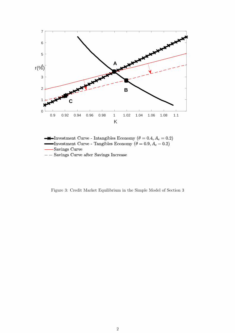
0.9 0.92 0.94 0.96 0.98 1 1.02 1.04 1.06 1.08 1.1

K

0

1

2

3

4

5

6

7

r(%)A

C

B

Figure 3: Credit Market Equilibrium in the Simple Model of Section 3

2

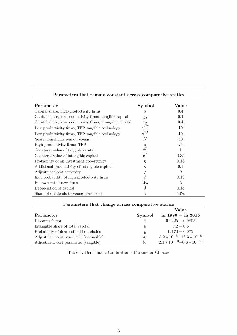
Parameters that remain constant across comparative statics

Parameter Symbol ValueCapital share, high-productivity firms α 0.4Capital share, low-productivity firms, tangible capital χI 0.4Capital share, low-productivity firms, intangible capital χT 0.4

Low-productivity firms, TFP tangible technology zu,Tt 10

Low-productivity firms, TFP tangible technology zu,It 10Years households remain young N 40High-productivity firms, TFP z 25

Collateral value of tangible capital θT 1

Collateral value of intangible capital θI 0.35Probability of an investment opportunity η 0.13Additional productivity of intangible capital κ 0.1Adjustment cost convexity ϕ 9Exit probability of high-productivity firms ψ 0.13Endowment of new firms W0 5Depreciation of capital δ 0.15Share of dividends to young households γ 40%

Parameters that change across comparative staticsValue

Parameter Symbol in 1980 − in 2015Discount factor β 0.9425− 0.9805Intangible share of total capital µ 0.2− 0.6Probability of death of old households % 0.170− 0.075Adjustment cost parameter (intangible) bI 3.2 ∗ 10−6−15.3 ∗ 10−6Adjustment cost parameter (tangible) bT 2.1 ∗ 10−10−0.6 ∗ 10−10

Table 1: Benchmark Calibration - Parameter Choices

3

0

2 0

4 0

6 0

8 0

%

0

2

4

6

8

%

­ 1 0 0

0

1 0 0

2 0 0

%

­ 5 0

0

5 0

1 0 0

%

0

1 0

2 0

3 0

% c

hang

e

0

1

2

3

4

% c

hang

e

= 0 .9 4 2 5   ­ ­ ­ ­> = 0 .9 8 0 5

= 0 .1 7 0   ­ ­ ­ ­ ­> = 0 .0 7 5

­ 2 0

­ 1 0

0

1 0

% c

hang

e

= 0 .9 4 2 5   ­ ­ ­ ­> = 0 .9 8 0 5

= 0 .1 7 0   ­ ­ ­ ­ ­> = 0 .0 7 5

­ 1 0

­ 5

0

5

% c

hang

e

= 0 .9 4 2 5   ­ ­ ­ ­> = 0 .9 8 0 5

= 0 .1 7 0   ­ ­ ­ ­ ­> = 0 .0 7 5

­ 2

­ 1

0

1

2

% c

hang

e

Figure 4: Simulation Exercise: households’propensity to save gradually increases because of(i) a decrease in the rate of time preference (β increases) and (ii) a decrease in the likelihood ofdeath of old households (% decreases) - comparison of the effects of the expansion in householdssavings in a tangibles economy (µ = 0.05) and an intangibles economy (µ = 0.65).

4

=0.9425  ­­­­> =0.9805=0.170  ­­­­­> =0.075

­5

0

5

10

15

20

25

% c

hang

e

=0.9425  ­­­­> =0.9805=0.170  ­­­­­> =0.075

0

0.5

1

1.5

2

2.5

3

% c

hang

e

Figure 5: Simulation Exercise: households’propensity to save gradually increases because of(i) a decrease in the rate of time preference (β increases) and (ii) a decrease in the likelihood ofdeath of old households (% decreases) - comparison of capital misallocation and TFP dispersionin a tangibles economy (µ = 0.05) and an intangibles economy (µ = 0.65).

5

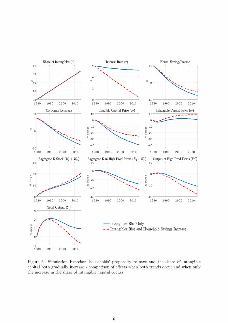
1980 1990 2000 201020

30

40

50

60

%

1980 1990 2000 20100

2

4

6

%

1980 1990 2000 2010­50

0

50

%

1980 1990 2000 2010­50

0

50

%

1980 1990 2000 2010

­40

­30

­20

­10

0

10

% c

hang

e

1980 1990 2000 2010

­40

­30

­20

­10

0

10

% c

hang

e

1980 1990 2000 20100

10

20

30

% c

hang

e

1980 1990 2000 2010­60

­40

­20

0

20

% c

hang

e

1980 1990 2000 2010­20

­10

0

10

% c

hang

e

1980 1990 2000 2010­1

0

1

2

3

% c

hang

e

Figure 6: Simulation Exercise: households’ propensity to save and the share of intangiblecapital both gradually increase - comparison of effects when both trends occur and when onlythe increase in the share of intangible capital occurs

6

198 0 198 5 199 0 199 5 200 0 200 5 201 0 201 5­7

­6

­5

­4

­3

­2

­1

0

1

2

3

% c

hang

e

Figure 7: Simulation Exercise: households’propensity to save and the share of intangible capitalboth gradually increase - comparison of effects on TFP when both trends occur, when only theincrease in the share of intangible capital occurs, and in a counterfactual partial equilibriumscenario

1980 1985 1990 1995 2000 2005 2010 2015­1

­0.5

0

0.5

1

1.5

2

%

Figure 8: Simulation Exercise: households’propensity to save and the share of intangible capitalboth gradually increase - comparison of effects when we shut down the debt overhang/savingschannel

7

APPENDICESFor Online Publication

A Robustness of Dispersion Evidence

A.1 Construction of the Intangible Capital Measure

We define intangible capital as the sum of knowledge capital and organizational capital.29 Fol-lowing Falato et al. (2014), we measure the former by capitalizing R&D expenses and the latterby capitalizing selling, general and administrative (SG&A) expenses weighted by 0.2.30 Theexpenditures are capitalized by applying the perpetual inventory method with a depreciationrate of 15% for R&D and 20% for SG&A. In order to get a measure for tangible capital, we alsouse the perpetual inventory method to capitalize tangible capital expenses with a depreciationrate of 15%. We drop firms that are observed only once and firms that are not observed ina continuous time period, and we exclude regulated, financial, and public service firms. Weconsider sectors at the 2-digit Standard Industrial Classification (SIC) level and drop thosewith less than 500 firm-year observations over the sample period. We measure output by sales,labor input by the number of employees, and total capital by the sum of capitalized tangibleand intangible capital.

TFP is defined as the residual of a Cobb-Douglas production function with a capital shareof income equal to 0.40. To control for outliers, we drop firms in the 1st and 99th percentilesof the distribution of labor productivity.

A.2 Robustness Checks

One alternative explanation of the results shown in Figures 1 and 2 in Section 2 could be thatthe sectors with a high intangibles share do not have a worse allocation of resources, but ratherare more dynamic and fast growing, and that the increase in dispersion of productivity reflectsthis higher dynamism. However, in Figure A, we show that sectors with high average salesgrowth have lower productivity dispersion in the whole sample period.

[FIGURE A ABOUT HERE]

[TABLE A ABOUT HERE]

Furthermore, Table A shows regression results where the dependent variable is a measureof productivity dispersion for each 2-digit sector-year observation. The regressors we considerare as follows: the dummy High share, which is equal to 1 if the sector belongs to the 50%2-digit industries with the highest average intangible share and which is equal to 0 otherwise;a time trend; and year and sector fixed effects. In columns 1 and 2, the dependent variable isthe dispersion in TFP. Column 1 includes year fixed effects and shows that the dispersion issignificantly larger for sectors with higher intangible share. Column 2 includes a time trend,interacted with the High share variable, and both sector and time fixed effects. It shows that the

29Falato et al. (2014) also consider informational capital. However, they state that their results do not dependon its inclusion. As informational capital can be measured only at the industry level but not at the firm levelusing Compustat data, we choose not to include this type of capital.30A portion of SG&A expenses captures expenditures that increase the value of intangible capital items such as

brand names and knowledge capital. Part of SG&A expenditures, however, does not affect the value of intangiblecapital, so Falato et al. (2014) follow Corrado, Hulten, and Sichel (2009) and assume that the portion relevantto intangible capital is around 0.2.

37

trend in dispersion over time is significantly more positive in the 50% most intangible sectorsthan in the other sectors, confirming the significance of the result shown in Figures 1 and 2.Similar results, across the two groups of high and low intangibles sectors, are obtained usinglabor productivity, as shown in columns 3 and 4.

B Derivation of the Simple Model

This appendix solves a simple partial equilibrium model that delivers the equations introducedin Section 3. Consider an infinite-horizon, discrete-time model of the final good-producingsector of an economy. Firms use capital, which is in constant aggregate supply K, to producea homogeneous consumption good. There are two types of firms, high-productivity and low-productivity, each composed of a continuum of mass 1. High-productivity firms live for 2 periods,and there are overlapping generations of these types of firms. Effi ciency in this economy isdetermined by the share ofK allocated to high-productivity firms. Our main interest is studyinghow exogenous interest rate variations affect the allocation of capital and aggregate outputdepending on the degree of tangibility of capital. This framework is extended in Section 4 in afull-fledged general equilibrium setup that can be used for realistic quantitative analysis.

B.1 High-Productivity Firms

Technology and FinancingHigh-productivity firms live for two periods, which we denote with y (young) and o (old). An

old firm that dies in period t− 1 leaves a a financial endowment or liability ae (−∞ < ae <∞),which translates into net worth ae(1 + rt) for the newborn young firm in period t. The youngfirm is able to produce ye units of the final good in period t, and has access to a technology toproduce the final good in period t+ 1 using the following linear production function:

ypt+1 = zt+1kt+1, (53)

where kt+1 represents capital purchased in t that produces output in t + 1, and zt+1 is aproductivity parameter. The firm can borrow bt+1 to purchase capital, subject to a constraint:

(1 + rt+1) bt+1 ≤ θqt+1kt+1, (54)

where 0 < θ ≤ 1. The collateral value of capital θ is the parameter in this stylized model thatcaptures capital tangibility. A shift toward a stronger reliance on intangible capital will becaptured as a decrease in θ. 31 Firms cannot issue equity.

The budget constraint for a high-productivity young firm is:

qtkt+1 = ae(1 + rt) + bt+1 + ye. (55)

31Note that a standard collateral constraint of the form

bt+1 ≤θqt+1kt+11 + rt+1

,

would not work when W0 < 0. This is because in that case the firm would have to be assumed to borrow morethan qt per unit of capital:

qt <θqt+11 + rt+1

,

to be able to purchase capital and pay down the debt, and by making the collateral constraint a function of kt+1,it would make the firm financially unconstrained, and the problem would not have a solution.

38

A mature firm realizes output, pays back any debts, sells its holdings of capital, and pays theresidual, net of the endowment for the next generation ae, as a dividend dt+1 to its shareholders:

dt+1 + ae = ypt+1 + qt+1kt+1 − bt+1 (1 + rt+1) .

Optimal SolutionProductive young firms in t = 0 maximize the present value of the dividend dt+1. We claim,

and later verify, that their marginal product of capital is greater than its user cost:

zt > qt −qt+1

1 + rt+1(56)

firms are credit constrained ((54) is binding), so that

kt+1 =ae(1 + rt) + ye

qt − θ qt+11+rt+1

. (57)

in which investment is equal to the total wealth available to invest divided by the downpay-ment necessary to purchase one unit of capital.

B.2 Low-Productivity Firms

There is a mass 1 of identical firms in the unproductive sector that produce the same homoge-neous final good as the high-productivity firms using a linear production function:

yut = zut ku,t, (58)

where ku,t represents capital installed in period t− 1 that produces output in period t, and zutis a productivity parameter. This sector is assumed to be financially unconstrained, and to payout all profits as dividends:

dut = yut − qt(kut+1 − kut

)(59)

to their shareholders every period.

B.3 Aggregation

From (57) it follows that the aggregate stock of capital held by the high-productivity firms is

Kt+1 =Ae(1 + rt) + Y e

qt − θ qt+11+rt+1

.

and aggregate output is

Yt = Y pt + Y u

t + Y e = ztKt + zut(K −Kt

).

Under the assumption that the high-productivity firms have the highest return on capital(zt > zut ), but their resources are insuffi cient to absorb all the capital, Kt+1 < K , it followsthat the low-productivity firms are willing to absorb all the capital not demanded by the high-productivity firms at a price equal to their marginal return on capital. the price of capitalis:

qt = zu +1

1 + rt+1 + ξqt+1, (60)

which, together with the assumption that zt > zut , proves the claim (56). ξ ≥ 0 is a wedge

39

that reduces the sensitivity of the price of capital to the interest rate, and summarizes theeffect of factors included in the full model developed later, such as decreasing marginal returnto capital in the unproductive sector.

B.4 Steady State

We consider a steady state equilibrium and drop reference to the time subscript t. Total outputis

Y = Y p + Y u + Y e = zK + zu(K −K

). (61)

Aggregate capital holdings of the high-productivity firms in the steady state are:

K =Ae(1 + r) + Y e

q(

1− θ1+r

) , (62)

where

q =zu

r + ξ. (63)

Equations (1), (2), and (3) in the steady state equilibrium of Section 3 correspond to equa-tions (61), (62) and (63) in this section.

C Optimal Dividend and Cash Accumulation Policy

Given equation (13), the first order condition for cash holdings af,t+1 for non investing firms is:

(1 + λt) = (1− ψ)[η(1 + λ+

t+1 + ϑt) + (1− η) (1 + λ−t+1 + ϑt)]

+ ψ. (64)

If we substitute (64) recursively forward, it is clear that if the firm expects ϑt to be positivenow or in the future, then λt > 0, and a non-investing firm will always retain all earnings anddt = 0. It is important to note that this is so because there is no cost of holding cash.

D Households

We derive below the solution of households’optimization problem under the steady state, so thatwages, dividends and interest rate are constant. Households have log utility. A representativeold household still living at time t maximizes the following objective function:

V ot (bot ) = max

cot ,bot+1

∞∑j=0

(1− %)jβj log (ct+j) (65)

subject to

cot = bot+1 + (1− γ)d− (1 + r)

(1− %)bot .

Working backward, we next consider the optimization problem of a young agent of age Nin period t, who will become old in period t+ 132:

V yt,N

(byt,N

)= max

cyt,N ,bot+1

u(cyt,N

)+ β(1− %)V o

t+1

(bot+1

)(66)

32We assume that an agent can also die with probability % in the transition between young and old.

40

subject tocyt,N = γd+ wTOT − (1 + r)byt,N + bot+1. (67)

where wTOT is defined as:wTOT ≡ w + wuI + wuT

Then we consider the optimization problem for a young household of age j < N :

V yt,j

(byt,j

)= max

cyt,j ,byt+1,j+1

u(cyt,j

)+ βV y

t+1,j+1

(byt+1,j+1

)(68)

subject tocyt,j = γd+ wTOT − (1 + r)byt,j + byt+1,j+1 (69)

D.1 Individual Problem of Old Households

We follow Blanchard (1985) and Yaari (1965) in assuming that households participate in a lifeinsurance scheme when old. The insurance scheme works within a cohort so that the survivorswithin a cohort pay the debt of the dying (if they are in debt) or, alternatively, receive thesavings of the dying. An old household begins a period with net debt (1 + rt)b

ot . The insurance

contract specifies that the % fraction of old households that die transfer their assets (or debt)(1 + rt)b

ot to the life insurer. Among the fraction (1− %) of households that survive, if they are

net savers (bot < 0), then they receive a return 11−%(1 + rt)b

ot on their assets, while, if they are

net debtors (bot > 0), they make a payment of 11−%(1 + rt)b

ot to the life insurer.

The first order condition with respect to bot+1 is

cot+1 = β(1 + r)cot . (70)

We guess a consumption policy rule:

cot = ∆d+ Θbot ,

and plug it into the FOC

∆d+ Θ

[cot − (1− γ) d+

(1 + r)

(1− %)bot

]= β(1 + r) (∆d+ Θbot )

cot =

[β(1 + r)∆

Θ+ (1− γ)− ∆

Θ

]d+ (1 + r)

[β − 1

(1− %)

]bot ,

and then solve for the unknown coeffi cients

∆ =β(1 + r)∆

Θ+ (1− γ)− ∆

Θ

Θ = (1 + r)

[β − 1

(1− %)

]

∆ =β∆[

β − 1(1−%)

] + (1− γ)− ∆

(1 + r)[β − 1

(1−%)

]∆ =

(1− γ) (1 + r) [1− β(1− %)]

%+ r

41

The policy rule is:

cot = (1− (1− %)β)

[(1− γ)(1 + r)

(%+ r)d− (1 + r)

(1− %)bot

]. (71)

and the evolution of the wealth of old households is given by

bot+1 =(1− %) [1− β(1 + r)]

(%+ r)(1− γ)d+ (1 + r)βbot , (72)

which says that old households slowly consume their savings if β(1 + r) < 1, and do so at afaster rate the higher the dividends. In our simulations typically β(1 + r) < 1.33

D.2 Individual Problem of Young Households

We first consider the optimization problem of an agent of age N in period t, who will becomeold in period t+ 1:

V yt,N

(byt,N

)= max

cyt,N ,bot+1

u(cyt,N

)+ β(1− %)V o

t+1

(bot+1

)(73)

such that:cyt,N = γd+ wTOT − (1 + r)byt,N + bot+1. (74)

The first order condition implies that

1

cyt,N+ β

(∂V o

t+1

(bot+1

)∂bot+1

+∂V o

t+1

(bot+1

)∂bot+2

∂bot+2

∂bot+1

)= 0.

And applying the envelope theorem we obtain:

cot+1 = β (1 + r) cyt,N .

We substitute cot+1 using (71) and we obtain:

cyt,N =

(1

β− (1− %)

)((1− γ)d

(%+ r)−

bot+1

(1− %)

). (75)

Then we consider the optimization problem for a young household of age j<N :

V yt,j

(byt,j

)= max

cyt,j ,byt+1,j+1

u(cyt,j

)+ βV y

t+1,j+1

(byt+1,j+1

), (76)

such that:cyt,j = γd+ wTOT − (1 + r)byt,j + byt+1,j+1, (77)

which yields the standard Euler equation:

cyt,j = [β(1 + r)]−(N−j) cyt+N−j,N . (78)

Equations (75) and (78) fully characterize the life-cycle path of consumption of a household

33To see this more clearly, denote a = −b as savings, and write

aot+1 = (1 + r)βaot −(1− %) [1− β(1 + r)]

(%+ r)(1− γ)d.

42

as a function of its assets when entering old age in period t+ 1, bot+1.

D.3 Value of Savings of Oldest Young: bot+1

We use the above equations, the budget constraint (69), and the assumption that newbornhouseholds have no endowment (byt,1 = 0) to determine the value of savings for retirementbot+1 ≡ b

yt+1,N+1.

We use the budget constraint for j = 1 (a young household of age = 1), in which the debtbrought over, byt,1, is zero:

byt,1 =

(γd+ wTOT

)− cyt,1 + byt+1,2

(1 + r)= 0,

and we solve forward:

byt,1 =

(γd+ wTOT

)− cyt,1

(1 + r)+

(γd+ wTOT

)− cyt+1,2 + byt+2,3

(1 + r)2

=(γd+ wTOT

) N∑j=1

1

(1 + r)j−

N∑j=1

cyt+j−1,j

(1 + r)j+byt+N,N+1

(1 + r)N

Making use of the FOC:

cyt,j = [β(1 + r)]−(N−j) cyt+N−j,N (79)

we get

cyt,j = [β(1 + r)]−(N−j) cyt+N−j,N

cyt,1 = [β(1 + r)]−(N−1) cyt+N−1,N

cyt+1,2 = [β(1 + r)]−(N−2) cyt+1+N−2,N = [β(1 + r)]−(N−2) cyt+N−1,N

cyt+2,3 = [β(1 + r)]−(N−3) cyt+2+N−3,N = [β(1 + r)]−(N−3) cyt+N−1,N

cyt+N−1,N = [β(1 + r)]−(N−N) cyt+N−1+N−N,N = cyt+N−1,N ,

and plug in and simplify

N∑j=1

cyt+j−1,j

(1 + r)j=

cyt,1(1 + r)

+cyt+1,2

(1 + r)2 +cyt+2,3

(1 + r)3 + ...+cyt+N−1,N

(1 + r)N

=cyt+N−1,N

(1 + r)N

N−1∑j=0

β−(N−1−j)

= −cyt+N−1,N

(1 + r)NβN − 1

βN−1 (β − 1).

We substitute back in and keep simplifying

byt,1 =(γd+ wTOT

) 1

r

[1− 1

(1 + r)N

]−cyt+N−1,N

(1 + r)NβN − 1

βN−1 (β − 1)+byt+N,N+1

(1 + r)N

43

0 =(γd+ wTOT

) 1

r

[(1 + r)N − 1

]−(

1

β− (1− %)

)βN − 1

βN−1 (β − 1)

(1− γ)d

(%+ r)

+

[(1

β− (1− %)

)1

(1− %)

βN − 1

βN−1 (β − 1)+ 1

]byt+N,N+1(

1

β− (1− %)

)βN − 1

βN−1 (β − 1)

(1− γ)d

(%+ r)−(γd+ wTOT

) 1

r

[(1 + r)N − 1

]=

[(1

β− (1− %)

)1

(1− %)

βN − 1

βN−1 (β − 1)+ 1

]byt+N,N+1

Finally, we solve to get:

−byt+N,N+1 =

(γd+ wTOT

)1r

[(1 + r)N − 1

]−Ψ (1−γ)d

(%+r)

Ψ1−% + 1

(80)

Ψ ≡(

1

β− (1− %)

)βN − 1

βN−1 (β − 1)

Equation (80) is very intuitive. Savings for retirement −bot+1 increase in the differencebetween income before and after retirement. Moreover, an increase in life expectancy (a dropin %) reduces the value of the term Ψ and therefore increases −bot+1.

D.4 Aggregate Savings of the Young

The previous section determines a sequence of optimal consumption at every age, cyt,1, ..., cyt,N ,

and applying the budget constraint (69) we can determine a sequence of assets for every agebyt,2, ..., b

yt,N , which is constant for every period t. In equilibrium there is a measure 1 of house-

holds, a fraction φφ+% old, and a fraction

%φ+% young. Moreover there is a measure

%φ+%

1N of

young households for each age. Therefore, after dropping the subscript t, we can define aggre-gate savings of the young households as:

By =%

φ+ %

1

N

N∑j=1

byj+1. (81)

Savings of a young household are:

byj+1 = cyj − γd− wTOT + (1 + r)byj (82)

We solve for byN (from now on for simplicity omit the superscript y) :

bN =1

1 + r

(γd+ wTOT

)− 1

1 + rcN +

1

1 + rbN+1, (83)

where both bN+1 and cN are determined by (75) and (80) above. At age N − 1 (we usect = [β(1 + r)]−1 ct+1):

bN−1 =1

1 + r

(γd+ wTOT

)− 1

1 + rcN−1 +

1

1 + r

[1

1 + r

(γd+ wTOT

)− 1

1 + rcN +

1

1 + rbN+1

]

44

bN−1 =1

1 + r

(γd+ wTOT

)− 1

1 + r[β(1 + r)]−1 cN

+1

1 + r

[1

1 + r

(γd+ wTOT

)− 1

1 + rcN +

1

1 + rbN+1

]=

1

1 + r

(γd+ wTOT

)+

1

(1 + r)2

(γd+ wTOT

)− 1

1 + r[β(1 + r)]−1 cN −

1

(1 + r)2 cN +1

(1 + r)2 bN+1

=

(1

1 + r+

1

(1 + r)2

)(γd+ wTOT

)−(

1

β+ 1

)cN

(1 + r)2 +1

(1 + r)2 bN+1,

and therefore at age N − 2 :

bN−2 =1

1 + r

(γd+ wTOT

)− 1

1 + rcN−2 +

1

1 + rbN−1

=1

1 + r

(γd+ wTOT

)− 1

1 + r[β(1 + r)]−1 [β(1 + r)]−1 cN

+1

1 + r

((1

1 + r+

1

(1 + r)2

)(γd+ wTOT

)−(

1

β (1 + r)2 +1

(1 + r)2

)cN +

1

(1 + r)2 bN+1

)=

(1

1 + r+

1

(1 + r)2 +1

(1 + r)3

)(γd+ wTOT

)−(

1

β2 +1

β+ 1

)cN

(1 + r)3 +1

(1 + r)3 bN+1,

and at a generic age N − t :

bN−t =

t∑j=0

γd+ wTOT

(1 + r)j+1− cN

(1 + r)t+1

t∑j=0

1

βj+

bN+1

(1 + r)t+1 (84)

We use general formulas:∞∑j=0

xj = 11−x and

t∑j=0

xj =(1− xt+1

)1

1−x , ort∑

j=0

1(1+r)j

=

(1− 1

(1+r)t+1

)1+rr and

t∑j=0

1(1+r)j+1

=(

1− 1(1+r)t+1

)1r , so that

t∑j=0

γd+ wTOT

(1 + r)j+1=

(1− 1

(1 + r)t+1

)γd+ wTOT

r

cN

(1 + r)t+1

t∑j=0

1

βj=

cN

(1 + r)t+1

(1− 1

βt+1

)β

β − 1

hence:

bN−t =

(1− 1

(1 + r)t+1

)γd+ wTOT

r− cN

(1 + r)t+1

(1− 1

βt+1

)β

β − 1+

bN+1

(1 + r)t+1 (85)

45

Now we add up the savings/borrowing over all ages from b2 to bN to get:

N−2∑t=0

bN−t =γd+ wTOT

r

N−2∑t=0

(1− 1

(1 + r)t+1

)− β

β − 1cN

N−2∑t=0

(1

(1 + r)t+1

(1− 1

βt+1

))

+bN+1

N−2∑t=0

(1

(1 + r)t+1

)The value of each summation term is:

N−2∑t=0

(1− 1

(1 + r)t+1

)= −1

r

(r − (r + 1)−N+1 −Nr + 1

)= −1

r

(1 + r(1−N)− 1

(1 + r)N−1

)

=1

r

(1

(1 + r)N−1+ r(N − 1)− 1

)

N−2∑t=0

(1

(1 + r)t+1

(1− 1

βt+1

))=

N−2∑t=0

1

(1 + r)t+1 −N−2∑t=0

(1

[(1 + r)β]t+1

)

=1− (1 + r)−N+1

(1 + r)− 1− 1− [(1 + r)β]−N+1

[(1 + r)β]− 1

N−2∑t=0

(1

(1 + r)t+1

)=

1− (1 + r)−N+1

(1 + r)− 1

Substituting them back:

N−2∑t=0

bN−t =γd+ wTOT

r

1

r

(1

(1 + r)N−1+ r(N − 1)− 1

)

− β

β − 1cN

[1− (1 + r)−N+1

(1 + r)− 1− 1− [(1 + r)β]−N+1

(1 + r)β − 1

]+ bN+1

1− (1 + r)−N+1

(1 + r)− 1

We rename terms:

N−2∑t=0

bN−t = A1γd+ wTOT

r−A2cN +A3bN+1

A1 ≡ 1

r

(1

(1 + r)N−1+ r(N − 1)− 1

)

A2 ≡ β

β − 1

[1− (1 + r)−N+1

(1 + r)− 1− 1− [(1 + r)β]−N+1

(1 + r)β − 1

]

A3 ≡ 1− (1 + r)−N+1

(1 + r)− 1

46

D.5 Aggregate Savings of the Old

In equilibrium there are %φ+%

1N households that become old every period, and %

φ+%1N (1 − %)j

households that survived for j periods . Therefore aggregate savings of the old households are:

Bo =%

φ+ %

1

N

∞∑j=1

(1− %)jb0j (86a)

also note that b01 is the initial savings from young age as defined in (80)Recall that (from (72)):

boj+1 = A+ β(1 + r)boj , (87)

and

A ≡ (1− %) [1− β(1 + r)]

(%+ r)(1− γ)d,

so that:bo2 = A+ β(1 + r)bo1, (88)

bo3 = A+ β(1 + r)bo2 = A+ β(1 + r)A+ β2(1 + r)2bo1, (89)

bot = A+ β(1 + r)A+ ...+ βt−2(1 + r)t−2A+ βt−1(1 + r)t−1bo1, (90)

bot = A

t−2∑j=0

βj(1 + r)j

+ βt−1(1 + r)t−1bo1, (91)

bot =(β (1 + r))t−1 − 1

β (1 + r)− 1A+ [β(1 + r)]t−1 bo1, (92)

∞∑t=1

(1− %)tb0t =∞∑t=1

(1− %)t

[(β (r + 1))t−1 − 1

β (1 + r)− 1A+ [β(1 + r)]t−1 bo1

]

=A

β (1 + r)− 1

∞∑t=1

(1− %)t[(β (r + 1))t−1 − 1

]+ bo1

∞∑t=1

(1− %)t [β(1 + r)]t−1

=

[A

β + rβ − 1+ bo1

] ∞∑t=1

(1− %)t (β (r + 1))t−1 − A

β + rβ − 1

∞∑t=1

(1− %)t

=

[A

β + rβ − 1+ bo1

]1

β(1 + r)

∞∑t=1

[(1− %)β(1 + r)]t − A

β + rβ − 1

∞∑t=1

(1− %)t,

∞∑t=1

[(1− %)β(1 + r)]t =1

1− (1− %)β(1 + r)− 1 =

(1− %)β(1 + r)

1− (1− %)β(1 + r),

and ∞∑t=1

(1− %)t =1

1− 1 + %− 1 =

1− %%

.

Finally:

∞∑t=1

(1− %)tb0t =

[A

β + rβ − 1+ bo1

](1− %)

1− (1− %)β(1 + r)− A

β + rβ − 1

1− %%

47

D.6 Summing Up Aggregate Household Borrowing

Aggregate household borrowing is:B = Bo +By (93)

where savings of the old is:

Bo =%

φ+ %

1

N

[(A

β + rβ − 1+ bretirement

)(1− %)

1− (1− %)β(1 + r)− A

β + rβ − 1

1− %%

]and

A ≡(

(1− %) (1− (1 + r)β)

(%+ r)

)(1− γ)d,

bretirement ≡Ψ (1−γ)d

(%+r) −(γd+ wTOT

)1r

[(1 + r)N − 1

]Ψ

1−% + 1,

and

Ψ ≡(

1

β− (1− %)

)βN − 1

βN−1 (β − 1).

And savings of the young is:

By =%

φ+ %

1

N

N−2∑t=0

bN−t =%

φ+ %

1

N

[A1γd+ wTOT

r−A2cN +A3b

retirement

],

where

A1 ≡ 1

r

(1

(1 + r)N−1+ r(N − 1)− 1

),

A2 ≡ β

β − 1

[1− (1 + r)−N+1

(1 + r)− 1− 1− [(1 + r)β]−N+1

(1 + r)β − 1

],

A3 ≡ 1− (1 + r)−N+1

(1 + r)− 1,

and

cN =

(1

β− (1− %)

)((1− γ)d

(%+ r)− bretirement

(1− %)

).

48

For Online Publication(Appendix Tables and Figures)

1

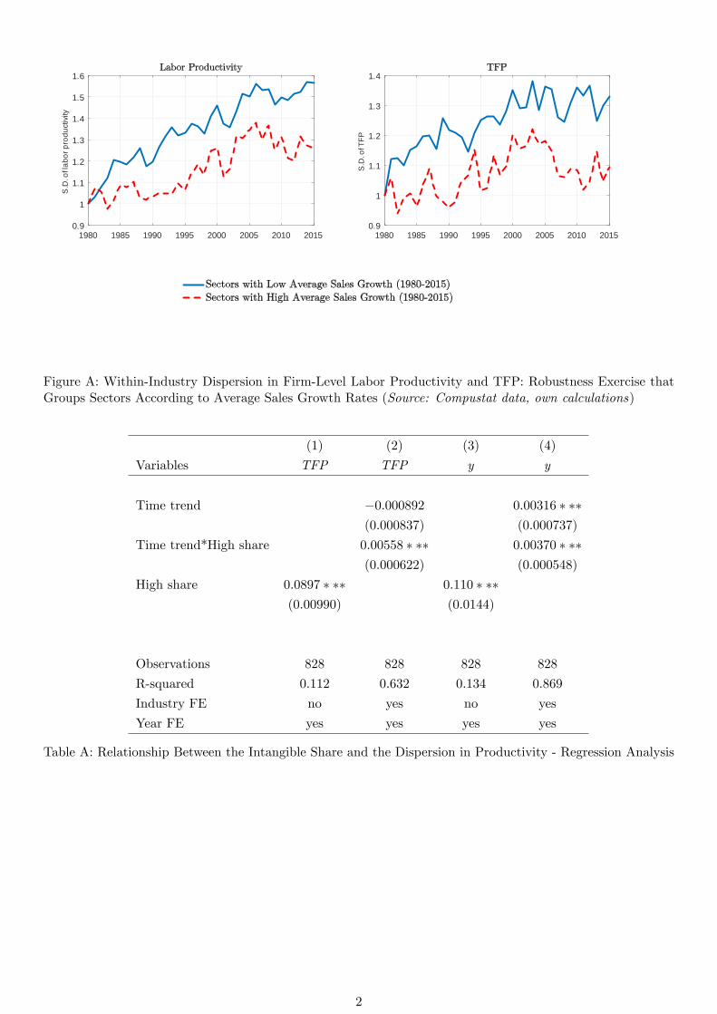
1980 1985 1990 1995 2000 2005 2010 20150.9

1

1.1

1.2

1.3

1.4

1.5

1.6S

.D. o

f lab

or p

rodu

ctiv

ity

1980 1985 1990 1995 2000 2005 2010 20150.9

1

1.1

1.2

1.3

1.4

S.D

. of T

FP

Figure A: Within-Industry Dispersion in Firm-Level Labor Productivity and TFP: Robustness Exercise thatGroups Sectors According to Average Sales Growth Rates (Source: Compustat data, own calculations)

(1) (2) (3) (4)

Variables TFP TFP y y

Time trend −0.000892 0.00316 ∗ ∗∗(0.000837) (0.000737)

Time trend*High share 0.00558 ∗ ∗∗ 0.00370 ∗ ∗∗(0.000622) (0.000548)

High share 0.0897 ∗ ∗∗ 0.110 ∗ ∗∗(0.00990) (0.0144)

Observations 828 828 828 828

R-squared 0.112 0.632 0.134 0.869

Industry FE no yes no yes

Year FE yes yes yes yes

Table A: Relationship Between the Intangible Share and the Dispersion in Productivity - Regression Analysis

2