wage equalization and regional misallocation: evidence
TRANSCRIPT

WAGE EQUALIZATION AND REGIONALMISALLOCATION: EVIDENCE FROM ITALIANAND GERMAN PROVINCES
Tito BoeriBocconi University
Andrea IchinoEuropean University Instituteand University of Bologna
Enrico MorettiUniversity of California, Berkeley
Johanna PoschAnalysis Group
AbstractItaly and Germany have similar geographical differences in �rm productivity — with the North moreproductive than the South in Italy and the West more productive than the East in Germany — but haveadopted different models of wage bargaining. Italy sets wages based on nationwide contracts thatallow for limited local wage adjustments, while Germany has moved toward a more �exible systemthat allows for local bargaining. We �nd that Italy exhibits limited geographical wage differences innominal terms and almost no relationship between local productivity and local nominal wages, whileGermany has larger geographic wage differences and a tighter link between local wages and localproductivity. As a consequence, in Italy, low productivity provinces have higher non-employmentrates than high productivity provinces, because employers cannot lower wages, while in Germanythe relationship between non-employment and productivity is signi�cantly weaker. We concludethat the Italian system has signi�cant costs in terms of forgone aggregate earnings and employmentbecause it generates a spatial equilibrium where workers queue for jobs in the South and remainunemployed while waiting. If Italy adopted the German system, aggregate employment and earningswould increase by 11.04% and 7.45%, respectively. Our �ndings are relevant for other Europeancountries. (JEL: J3, J5)
1. Introduction
Wage inequality is large and rising in many countries. Different countries have differentlabor market institutions to mitigate labor market inequality, including minimumwages, subsidies for low wage workers like the Earned Income Tax Credit, and unionscontracts.
In Western European countries, multi-�rm collective bargaining agreements arecommon practice and cover the majority of workers. In 12 Western European countries
Acknowledgments: We thank Rosario Ballatore, Michael Burda, Zach Bleemer, Christian Dustmann,Daniela Vuri and seminar participants at the Fondazione De Benedetti, the OECD, CEPR-ESSLE,SOLE-EALE-2020, ECB and the Universities of Berkeley, Rome "La Sapienza", Collegio CarloAlberto,University of Zurich and the EUI for helpful comments and suggestions. We are also grateful to MichelaFinizio of Sole24Ore, for sharing the data we used in Section V.E.
E-mail: [email protected] (Boeri); [email protected] (Ichino); [email protected](Moretti); [email protected] (Posch)
Journal of the European Economic AssociationPreprint prepared on March, 2021 using jeea.cls v1.0.

Boeri, Ichino, Moretti & Posch Wage Equalization and Regional Misallocation 2
out of 18, multi-�rm collective bargaining covers more than 70% of the workers. Onlyin Ireland (where there is, however, strong co-ordination at the industry level) and inthe UK, plant-level agreements are dominant in the structure of bargaining (OECD2017) although the two countries differ on how binding their national agreements are(Du Caju et al. 2008). Typically, �rms and unions belonging to a speci�c sector bargainover an occupation-speci�c wage schedule. This wage schedule applies to all workersin that sector, irrespective of their location and of whether or not they belong to aunion.1
The objective of collective bargaining is to equalize salaries across employers,"levelling the playing �eld across �rms" (OECD 2018), and reducing inequality. A vastliterature on collective bargaining (Flanagan 1999) and on the determinants of incomedistributions (Atkinson and Brandolini 2006) considers centralized wage setting aninstitution that reduces earning and income inequalities.
In this paper, we investigate an important but under-researched feature of collectivebargaining systems. We argue that while centralized wage bargaining may besuccessful at compressing nominal wage inequality in a country, it can also createcostly imbalances between cities and regions, with negative correlations betweenreal wages and productivity, as well as higher income inequality. In the presenceof geographic differences in productivity across cities and regions, nominal wageequalization across localities can lead to lower employment and earnings in lowproductivity areas and in the aggregate.
We study the local and aggregate effects of national wage bargaining systemsin Italy and Germany. Italy and Germany represent two useful case studies. Bothmake extensive use of collective bargaining agreements, but the level of resultingwage �exibility is markedly different. Italian nationwide sectoral contracts are morebinding and allow for only limited local wage adjustments. This means that within eachsector, �rms in high productivity and low productivity areas face largely the same wageschedule.2 The German system is also based on sectoral wage bargaining. Contrary toItaly however, German institutions allow for signi�cant �exibility in wage setting at the�rm level. This �exibility has been widely used in dealing with the large productivitydifferential between eastern and western �rms after German reuni�cation.
In the �rst part of the paper, we study the relationship between local �rmproductivity and local wages, non-employment rates, and cost of living. Ourgeographic unit of analysis is a local labor market, de�ned as an Italian "Province"
1. As acknowledged by Card et al. (2004), there is de facto no distinction between union and nonunionsectors in these countries. Most countries have "excess coverage" of collective bargaining, that is, they havea fraction of workers involved by the agreements negotiated by the unions (coverage) which is signi�cantlylarger than the fraction of workers members of a trade union (union density). Excess coverage is presentin Austria, Belgium, Denmark, Finland, France, Germany, Greece, Iceland, Ireland, Italy, Luxembourg,Netherlands, Norway, Portugal, Slovenia, Spain, Sweden and Switzerland (OECD 2017).
2. While �rms can increase wages above the national contract schedule, they cannot lower them in mostcases. We provide details on these institutions in the next Section.
Journal of the European Economic AssociationPreprint prepared on March, 2021 using jeea.cls v1.0.

Boeri, Ichino, Moretti & Posch Wage Equalization and Regional Misallocation 3
(103 in total) or a German "Spatial Planning Region –"Raumordnungsregion" (96 intotal).
Empirically, Italy and Germany have a similar cross-province standard deviationin mean �rm productivity, as measured by �rm value added. In Italy, �rm value addedis signi�cantly higher in the North than in the South: in 2014, the gross value added perworker in an average �rm of Milano, for example, was 71% above the value added in anaverage �rm of Cosenza, in the southern region of Calabria. In Germany, productivityis signi�cantly higher in the West than in the East: the value added per worker in anaverage �rm in Munich is 83% above the value added in an average �rm of NorthThuringen in East Germany.3 In Italy, the North-South productivity gap re�ects long-lasting historical differences in transportation infrastructure, distance from Europeanmarkets, ef�ciency of local governments and local policies, criminal activity, andcultural norms, while in Germany, the East-West gap likely re�ects half a century ofCommunist rule in the East as well as other historical factors.4
While Italy and Germany have similar geographic distribution of �rm productivity,they have important differences in the geographic distribution of nominal wages, likelyre�ecting wage bargaining differences in the two countries. In Italy, there is a muchstronger degree of wage equalization across provinces than in Germany. For example,after controlling for worker characteristics the 90-10 percentile difference in meanwages across provinces is 43.3% in Germany, more than four times larger than the10.3% difference in Italy. The mean wage difference between the North and the Southin Italy is 4.3%, while the mean West-East difference in Germany is seven times larger:29.7%, despite similar productivity differences.
Crucially, we �nd a marked difference in the relationship between localproductivity and local nominal wages in the two countries. If wages can fully adjust,we should see a tight relationship between the two, with areas that enjoy higher �rmproductivity also having proportionally higher mean nominal wages. This is indeedthe case in the US (Hornbeck and Moretti 2018). By contrast, if wages are preventedfrom fully adjusting, we should see a weaker relationship. In the extreme case of fully-binding national contracts with complete nominal wage equalization, we should seeno relationship at all. When we regress log mean nominal wage (adjusted for workerscharacteristics) on log value added across provinces, we �nd an elasticity of wages
3. Similar geographic differences exist in most countries. In the US, total factor productivity of �rms incities at the top of the TFP distribution is double that of cities at the bottom of the distribution (Hornbeckand Moretti 2018).
4. It is worth emphasizing that the North-South productivity gap in Italy is remarkably similar to theWest-East productivity gap in Germany. In 2014, the difference in mean value added between the NorthernItalian and Southern Italian �rms was 19.0%. The corresponding difference between West and East German�rms was almost identical: 19.9%. In this paper, we will take these differences as given. Our analysis willfocus on the effects of these differences, rather than on their causes. The literature on regional productivitydifferences is immense. Examples for Italy include Ban�eld 1958, Putnam et al. 1993, Ichino and Maggi2000, Guiso et al. 2004 and, more recently, Buonanno et al. 2015, Bigoni et al. 2016, Adda 2018. Anexample for Germany is Burda and Hunt 2001).
Journal of the European Economic AssociationPreprint prepared on March, 2021 using jeea.cls v1.0.
Boeri, Ichino, Moretti & Posch Wage Equalization and Regional Misallocation 4
with respect to value added of 0.20 in Italy and 0.74 – almost four times larger – inGermany.
Thus, German �rms are signi�cantly more able to adjust nominal wages to localproductivity than Italian �rms.
A simple model indicates that wage bargaining differences in the two countriesshould result in geographical differences of the distribution of non-employment rates,housing costs and real wages. First, in Italy, where wages cannot fully adjust, provinceswith low productivity should have higher non-employment rates because their �rmsneed to pay wages above the local market-clearing level. This should be less true inGermany, where wages can adjust to local productivity. When we regress local non-employment rate on local value added we �nd that the elasticity of non-employmentrates with respect to value added is negative in both countries – indicating thatprovinces with lower value added have higher non-employment rates – but the elasticityin Italy is -1.43 (0.03), almost six times larger (in absolute value) than Germany’s -0.25(0.02) elasticity. Our �ndings are not driven by the existence of an informal sector inItaly.
Second, since workers can move across regions, low productivity provinces shouldhave lower housing prices, both in Italy and Germany. Empirically this is the case: we�nd a positive relationship between housing prices and local productivity.
Third, there are striking implications for real wages, de�ned as nominal wagesde�ated by the local cost of living. In Italy we �nd a negative relationship betweenreal wages and local value added. Despite having higher productivity, provinces inthe North have lower real wages than provinces in the South, since the South has lowhousing costs but similar nominal wages.5 By contrast, in Germany, we do not see thatreal wages in the West are lower than in the East, since nominal wages are spatiallymore �exible.
This means that employed Italians are better off working in the South in terms ofpurchasing power. However, the probability of having a job is higher in the North. Oneway to think about geographic differences in Italy is that national wage contracts havecreated a spatial equilibrium where workers queue for jobs in the South. If they �nda job, they are better off than their colleagues in the North in terms of real wages, butwhile queued they remain not-employed.
Overall, the current wage-setting system in Italy appears inef�cient. If nominalwages were allowed to re�ect local productivity, nominal wages would decline in lowproductivity provinces, and employment there would increase, resulting in an overallincrease in employment in the country.6
5. See Jappelli and Pistaferri (2000) for an analysis of how consumption inequality relates to incomeinequality in Italy.
6. If the elasticity of labor demand is larger than one, aggregate labor earnings would increase. Intuitively,an elastic labor demand means that the increase in employment in low productivity areas more than offsetsthe decline in wages. Labor demand – at least in the traded sector – is probably elastic in the case of anopen economy like Italy, which is fully integrated in European product markets.
Journal of the European Economic AssociationPreprint prepared on March, 2021 using jeea.cls v1.0.

Boeri, Ichino, Moretti & Posch Wage Equalization and Regional Misallocation 5
In the last part of the paper, we quantify the aggregate costs in terms of forgoneaggregate earnings and employment. We consider what would happen if Italy adopteda system similar to Germany’s. We provide estimates from a counterfactual scenarioin which the Italian relationships between wages and value added and between non-employment and value added are the same as those observed in Germany. To beclear, we do not assume that wages or employment or value added are the same inthe two countries; rather, we apply to Italy the elasticity of wages with respect tovalue added and the elasticity of non-employment with respect to value added thatwe estimate for Germany.7 We �nd that average wages in Southern provinces woulddecrease by an average of 5.8% (or 52 cents an hour), while Southern employmentwould increase by 12.85 percentage points. On net, aggregate earnings in Southernprovinces would increase on average by 16.7%, or €115 a month. Nationwide, weestimate that aggregate employment would increase by 5.77 percentage points andaggregate earnings would increase by 7.51%. This amounts to around €600 per yearfor each working-age adult. We also consider an alternative counterfactual scenariowhere we allow for full adjustment of local wages to local productivity, and �nd similarestimates.
We conclude that in the aggregate, allowing union contracts some degree oflocal �exibility would improve the ef�ciency of labor allocation in Italy, resulting inincreased employment and per capita labor income. There would also be distributionalconsequences, as currently-employed workers in the South would enjoy lower nominaland real wages.8
Our �ndings are relevant to countries other than Italy and Germany, as the Italianand German system are by no means unique. Broadly speaking, France, Belgium,Portugal, Finland, Iceland, and Slovenia have a system similar to the Italian model,while Austria, Denmark, the Netherlands, Norway and Sweden are closer to theGerman model (OECD, 2017 and 2019). Countries like Greece, Portugal and Spainhave recently moved from a bargaining system similar to Italy’s to a "controlleddecentralization" which is not unlike the German system. France has long debated thedesirability of a decentralized bargaining system, and such goal was part of the labormarket reforms proposed by President Macron in 2017, though it was subsequentlydropped due to strong union opposition. While the level of macroeconomic bene�tfrom such reforms is likely to vary from country to country depending on the extentof productivity differences across areas, it is reasonable to conclude that countrieswith binding national contracts would improve ef�ciency if they moved toward theGerman wage-setting model. Evidence on the controlled decentralization of collective
7. Speci�cally, we set the counterfactual wages and the counterfactual employment in each Italianprovince based on the province observed value added and the elasticity of wages with respect to valueadded and employment with respect to value added that we estimate for Germany.
8. We caution, however, that the welfare implications are unknown. A welfare analysis is outside thescope of this paper, as it would require, among other things, assessing the value of leisure for currentlynon-employers individuals.
Journal of the European Economic AssociationPreprint prepared on March, 2021 using jeea.cls v1.0.

Boeri, Ichino, Moretti & Posch Wage Equalization and Regional Misallocation 6
bargaining in Portugal suggests that it has increased employment growth in Portugalby up to 10 percentage points (Hijzen and Martins 2016).
This paper is part of a growing body of work that focuses on the causes andconsequences of misallocation.9 The US represents an interesting specular example ofspatial misallocation. In this country, little prevents nominal wages from adjusting.10
However local employment is de facto constrained in many high productivity cities,resulting in large spatial misallocation. Hsieh and Moretti (2019) have found largeef�ciency losses in the form of forgone output and earnings caused by land useregulations that limit housing supply in the most productive cities, thereby constrainingthe �ow of labor toward high-TFP locations. By contrast, in the Italian case nothingconstrains local employment or mobility, but local wages cannot adjust to local labordemand conditions.11
There is a large literature on North-South differentials in labor market and livingconditions in Italy. We are not the �rst to explore the role played by collectivebargaining in this context. For instance, Faini (1999) evaluates the role played by theremoval of the so-called "gabbie salariali". Our paper is also part of the literature oncentralized wage bargaining. While much research has been devoted to the effectsof centralized wage bargaining, and on the estimation of wage curves in Italy,Germany and other European countries12, the combined effects of bargaining onthe housing market, the cost of living, real wages, the geography of employmentand their aggregate costs have not previously been investigated. Belloc et al. (2018)build on our framework to estimate urban/rural wage premia for employees (subjectto collective bargaining) and self-employed individuals (not subject to collectivebargaining) �nding a signi�cant urban wage premium for the latter and not for theformer.
The paper is organized as follows. In Section 2 we describe the institutional settingand wage determination mechanisms in Italy and Germany. Section 3 presents ourtheoretical model and its predictions. Section 4 describes the data. Empirical evidenceis presented and discussed in Section 5. The aggregate costs of spatial wage rigidityare analyzed in Section 6. Section 7 concludes.
9. Restuccia and Rogerson (2017) provides a recent survey.
10. The federal minimum wage in the US is not as binding as national contracts in Europe. It only appliesto low-wage workers, while European national contracts de�ne wage �oors for all levels of employment,excluding top management. Moreover, in the US there is geographic variation in minimum wages, withstate- and city-level minimum wages signi�cantly more binding than the federal minimum wage.
11. Other authors have used similar models to measure the effect of state taxes (Fajgelbaum et al.2015), internal trade frictions (Redding 2013), infrastructure (Ahlfeldt et al. 2015), and land misallocation(Duranton and Puga 2014).
12. For example, Calmfors and Horn (1986), Brunello et al. (2000), Brunello et al. (2001), Boeri et al.(2001), Manacorda and Petrongolo (2001) and Belloc et al. (2018).
Journal of the European Economic AssociationPreprint prepared on March, 2021 using jeea.cls v1.0.

Boeri, Ichino, Moretti & Posch Wage Equalization and Regional Misallocation 7
2. Wage Setting Mechanisms in Italy, Germany and Other European Countries
We begin by describing the main features of the wage bargaining systems in Italy andGermany. We then discuss which among European countries have wage bargainingsystems close to the Italian or German model. We stress that the speci�cs of a givencountry’s labor market institutions are quite complex. We do not seek to provide acomprehensive description of all the features of the wage-setting systems in eachcountry, but try instead to distill the key relevant differences in our analysis, abstractingfrom less crucial details.
Italy. Wage bargaining institutions in Italy have been historically designed to achievestrong nominal wage compression.13 Today, national agreements between unions andemployers set wages for each industry and occupational level. Industries are de�nednarrowly: for instance, there are currently 34 contracts in the chemical industry, 31 intextiles, and 39 in food production. Overall, there are 346 national agreements, andthey cover 97.7% of dependent employment registered in the social security systemand 99.3% of �rms.
With limited exceptions, Italian �rms cannot pay a salary below the levelestablished at the national level, irrespective of their speci�c pro�tability andproduct demand conditions. Thus, despite large geographic differences in productivity,transportation infrastructure, geographic location, local public goods, and localgovernment effectiveness across different areas of the country, �rms in a given industryface the same wage �oors.14 In theory, the system does allow for some wage bargainingat a decentralized level, either at the �rm level or within local industry clusters("distretti industriali"). In practice, decentralized bargaining is limited because it isonly allowed to increase wages above the levels set by the national agreements.15
13. Until 1992, it was mainly the centralized indexation of wages to in�ation (Scala Mobile) that reducednominal wage dispersion across sectors, regions and skill levels. The indexation imposed the same absolute(as opposed to proportional) salary increase to all employees, independent of their salary. As a result,wage increases in percent terms were large at the bottom and small at the top of the distribution, resultingin strong compression over time as described by Erickson and Ichino (1994), Checchi and Lucifora(2002), Manacorda (2004) and Garnero (2018). This mechanism was abolished in 1992, and in 1993 theItalian government, the national trade unions, and the employer associations signed a new income policyagreement which is still in effect today.
14. In some exceptional circumstances of �rms facing particularly severe dif�culties, wages lower thanthose established at the national level may be allowed. These cases are limited by "opening", "hardship"or "inability to pay" clauses to exceptional circumstances such as severe macroeconomic or idiosyncraticshocks that make downsizing unavoidable. These provisions are rarely invoked before a �rm is in severedistress.
15. Decentralized bargaining is limited to a small number of large �rms, since the wage �oors imposedby the national contracts are typically high for small and medium size �rms. In a 1995-96 survey of arepresentative sample of 8,000 �rms with at least 10 employees in both the manufacturing and servicesectors, only 10% of the �rms reported engaging in �rm-level bargaining (IStat 2000). Since then thisshare has only declined (Casadio 2003, 2008 and Brandolini et al. 2007).Devicienti et al. (2019) documentthat the Italian wage structure is determined by centralized, industry-level, collective bargaining.
Journal of the European Economic AssociationPreprint prepared on March, 2021 using jeea.cls v1.0.

Boeri, Ichino, Moretti & Posch Wage Equalization and Regional Misallocation 8
In many cases, wages in national contracts are set close to the market clearing levelsin Northern regions. One reason is that Southern employers are not well representedin employer associations. Northern regions have a much larger number of �rms,especially in manufacturing, and dominate the process.16 Con�ndustria, the mainemployer association in manufacturing, collects almost 80% of its revenues in theNorth and is typically led by a Northern president. On the workers’ side, unions areless transparent on their data, but their membership also seems to be dominated byworkers from Northern and Central regions. By contrast, Southern employers andworkers do not often reach the critical mass enabling them to have a strong voice inmulti-employer bargaining. Empirically, most Northern provinces are generally closeto full employment in a typical non-recession year, while unemployment is invariablymuch higher in the South.
In practice, private sector Italian �rms do retain a limited degree of wage �exibility.National contracts allow limited geographic differentiation and some use of meritpay. In recent years, the diffusion of "Contratti di lavoro a tempo determinato" (�xedterm contracts) has increased the bargaining position of employers vis a vis a limitednumber of employees per �rm (Saggio et al. 2018). Firms can also pay employeesunder the table. Finally, there are also clauses in some industry-level contracts allowingfor temporary deviations from the sectoral minimum pay levels under exceptionalcircumstances and with the agreements of unions, but such cases are extremely limited.Thus, while one should expect wage compression, one should not expect nominalwages to be uniformly identical in the private sector. Wages in the public sector (13.6%of employment in 2015), on the other hand, are nationally uniform; wages of teachers,doctors, nurses, social security workers, police, and military personnel are the same inevery province for a given job description and level of seniority.17
Table 1 presents an actual example of an Italian wage agreement. This speci�cagreement applies to one occupational level ("Livello 1") in the construction sector("Contratto Collettivo Nazionale per i Lavoratori Edili") in 2016. Entries are based onof�cial �gures released by the Italian Ministry of Labor and Social Affairs and showthe degree of permitted labor cost differentiation across provinces for each speci�ccomponent of labor costs. The Table shows that the main components of labor costs –for example, the �oor and the indexation to in�ation – have no cross-province variation,while other components have limited cross-province variation. The bottom row showsthat, overall, the standard deviation of total labor costs across provinces allowed by the
16. According to the Ministry of Labor, 67% of the registered contracts are signed in just four Northernregions (Lombardia, Emilia Romagna, Veneto and Piemonte) while only less than 10% belong toagreements signed in Southern Italy.
17. As a reaction to the strong nominal wage compression imposed by national agreements, the pastfew years witnessed an increasing number of so-called "pirate contracts" engineered by a small group ofemployers and a labor consultant, involving a "fake union" created ad-hoc with the purpose of signing thecontract. This kind of agreement is, however, still very rare according to the National Council for Economyand Labor (CNEL 2018).
Journal of the European Economic AssociationPreprint prepared on March, 2021 using jeea.cls v1.0.
Boeri, Ichino, Moretti & Posch Wage Equalization and Regional Misallocation 9
agreement is only €0.62 out of a total average hourly cost of labor of almost €23. Inother words, the coef�cient of variation is only 2.5%.
Table 2 shows examples of geographic wage variations for two large private sectoremployers and one public sector employer. For con�dentiality, we cannot reveal thenames of the two private �rms. The previous Table referred to a wage agreementwhile this Table reports wages actually observed in the labor market, but the pictureis similar. The �rst row shows the median monthly salary at a large national bank.We report the median monthly salary of male bank tellers with 10 to 20 years ofseniority and �nd limited geographic variability across North, Center and South Italy.For example, in the Northern city of Milan mean earnings are €1,659 per month, whilein the Southern cities of Naples, Palermo and Bari they are €1,649, €1,677, and €1,670,respectively. In the second row we show corresponding �gures for a large nationalenergy distribution company, inclusive of bonuses and merit pay. In both cases, weuncover limited geographic differences. If anything, wages in the energy companyare slightly higher in the South, although for con�dentiality reasons we cannot reportwages for speci�c occupations. In the last row we show the salary for an elementaryschool teacher with 5 years of seniority. As in the rest of the public sector, there is novariation in the nominal wage across areas.18
These are motivating examples based on three speci�c cases. In Section 5 wewill present more systematic evidence on geographic wage heterogeneity for arepresentative sample of Italian workers based on labor survey data.
Germany. Germany offers an interesting case study to compare with Italy. Similarto Italy, the German system is based on sector level collective bargaining agreements(albeit in Germany on the region (or Länder) rather than national level) negotiatedbetween employer and union representatives.19 But the German collective bargainingsystem differs from the Italian one because it allows for more �exibility to respondto �rm level shocks. Indeed, it is at the discretion of �rms to recognise sector levelbargaining by joining an employer federation (Dustmann et al. 2009). Only in this casewill sector level agreements apply to all workers in the �rm, whether union membersor not. Moreover, even when recognizing sector level agreements, an employer maystill deviate from some features of the multi-employer agreement through an “openingclause”. With the agreement of the employee representatives at the workplace, undersome special circumstances, a �rm may pay lower wages or set longer workinghours than those set in the multi-employer agreement20. In the chemical industry,
18. In 2018 the Minister of Education has tried to introduce pay differentials among teachers in an attemptto �ll outstanding vacancies in Northern schools, while there are no vacancies in Southern schools.
19. A double af�liation principle applies for the extension of these contracts to all workers in a �rm:either the employer and the union chosen by the majority of workers should belong to the associations thatsigned the agreements (OECD 2017). This contributes to explain why the coverage of collective agreementsis substantially lower in Germany than in Italy.
20. Opening clauses were initially focused mainly on hours restrictions but later also affected wages.Although initially they were meant as a temporary measure for �rms in distress, they often became a
Journal of the European Economic AssociationPreprint prepared on March, 2021 using jeea.cls v1.0.

Boeri, Ichino, Moretti & Posch Wage Equalization and Regional Misallocation 10
for instance, an opening clause allows companies to reduce the collectively agreedwage by up to 10% for a limited period of time in order to save jobs or improvecompetitiveness.21
The need for �rms in post-uni�cation Germany to remain competitive in a globalenvironment, the threat of production moving to cheaper Eastern European countriesas well as job reallocation from manufacturing to services led to a decrease inthe coverage of sector level bargaining agreements and a shift to more �rm levelagreements (Dustmann et al. 2014). The decline in the coverage of sectoral levelcollective bargaining and the rise of opening clauses is quanti�ed in Table 3. Theultimate effect of this shift was a signi�cant increase in the decentralization of wage-setting in Germany.22 The decline in the importance of industry-level contracts inGermany after 1995 and the corresponding increase in the importance of �rm-levelwage-setting mechanisms have allowed a growing number of German �rms to setwages in line with their productivity.
Overall, the German system allows for larger wage dispersion across employers inthe same sector than the Italian system.
Other Countries. An analysis of the Italian and German bargaining systems hasimplications not just for Italy and Germany, but also for other countries. While thespeci�cs of each country labor market institutions are different, key aspects of theItalian and the German bargaining systems are present elsewhere.
For our purposes, the key difference between the Italian and German systemsis that the latter permits a much wider scope for decentralized bargaining thanthe former, allowing wages to vary as a function of local productivity. Within theOECD, countries with systems closer to Germany’s tend to leave room for �rm-levelbargaining and/or permit deviations or opt-outs from sectoral agreements under a broadset of circumstances. OECD (2018) calls this system "organized decentralization".According to the OECD, the countries that had a system of organized decentralizationin 2015 are Austria, Denmark, the Netherlands, Norway, and Sweden along withGermany (OECD 2018).
permanent feature in �rms that would not be competitive applying fully the industry level agreement(Dustmann et al. 2014)
21. Trade unions and employer associations retain the right to veto such deviating works agreements.Sectoral agreements also impose a number of conditions for derogations to apply: companies have todisclose their �nancial information allowing workers representatives to have enough time to scrutinizethe �nancial status of the �rm, and the derogation must be temporary.
22. The higher fraction of workers subject to opening clauses in the West, displayed in Table 3, maycome as a surprise since theory would predict a larger need for deviations from the sectoral contracts forEastern �rms. However, it should be noted that opening clauses do not only allow deviations in terms ofwages, but also for example working hours, �exibility of overtime arrangements, reductions of constraintsto workers mobility within the �rm and between jobs and tasks. These types of opening clauses havebeen relatively common since the mid 1980s (Kohaut and Schnabel 2007) and are frequent in the West onaverage. However, Brändle et al. (2011) shows that the share among all opening clauses that deal with wagesetting has increased dramatically since the mid-90s. The time trend displayed in Table 3 clearly shows thatthis increase in the use of opening clauses is more pronounced in the East.
Journal of the European Economic AssociationPreprint prepared on March, 2021 using jeea.cls v1.0.

Boeri, Ichino, Moretti & Posch Wage Equalization and Regional Misallocation 11
By contrast, countries with systems closer to Italy’s are countries where nationalindustry level agreements play a dominant role and deviations are either not possibleor only allowed for wage increases relative to sectoral agreements. According to theOECD, this group includes France, Iceland, Portugal, and Slovenia (OECD 2018).
In the wake of the Euro-area crisis, three countries – Spain, Portugal, and (to someextent) Greece – recently transitioned from a highly-centralized system towards a moredecentralized, German-style model. A comparison of the Italian and German systemcan be informative on the possible effects of these reforms.
More generally, many European countries have a two-tier bargaining structure inwhich sector-level bargaining can, in principle, be accompanied by plant-level or localarea bargaining. For example, in Denmark the proportion of �rms carrying out two-tierbargaining more than doubled between 1989 to 1995 (Traxler et al. 2001; Andersenet al. 2003). Similarly, the number of Belgian �rms involved in both industry and plant-level agreements increased tenfold from 1980 and the mid-1990s (Van Ruysseveldt andVisser 1996). Two-tier bargaining structures are also present in Austria, Finland, theNetherlands, Norway, and Sweden (Boeri et al. 2001).
3. Theoretical Framework
Both Italy and Germany have large spatial productivity differences. In Italy, nationalcontracts limit the ability of local wages to adjust to local productivity, while inGermany labor market reforms have allowed employers to adjust wages to localproductivity.
We present a simple spatial equilibrium model intended to provide intuition forthe effects of the Italian and German wage-setting systems and to guide our empiricalanalysis. The model is a standard Rosen-Roback model and is kept deliberately simple.The main objective is to compare the spatial equilibria under two extreme cases: (1)local nominal wages can freely adjust to local productivity, and (2) local nominalwages cannot adjust (due to institutional constraints) but workers and �rms are freeto relocate. Rosen-Roback models of spatial equilibria have traditionally focused onthe case of market clearing. The case where the labor market does not clear has notreceived much attention.23
In interpreting the model, two points need to be clear. First, while the modelprovides useful benchmarks, it should be clear that neither Germany nor Italy is exactlydescribed by either of these two extremes. While German �rms have some �exibility toset nominal wages more in line with local productivity levels, union contracts ensurethat this �exibility is not absolute. Similarly, while Italian �rms have less �exibilityin setting nominal wages, they nevertheless maintain some ability to adjust wages.Second, the focus is on geographic differences. Thus, we abstract from labor marketinstitutions that are uniform across the country, such as employment protection and
23. Kline and Moretti (2013) model a case where unemployment arises from search frictions.
Journal of the European Economic AssociationPreprint prepared on March, 2021 using jeea.cls v1.0.
Boeri, Ichino, Moretti & Posch Wage Equalization and Regional Misallocation 12
unemployment bene�ts. While both Germany and Italy have important labor marketregulations of this variety, their effects are clearly outside the scope of this paper.
3.1. Setup
We consider two regions r D ¹n; sº that produce a traded good with a price set on theinternational market. Production in each region is given by:
Yr D ArK.1�˛/r E˛r (1)
whereAr denotes Total Factor Productivity (TFP);Er is employment andKr is capital.The two regions are ex-ante identical with the exception of their level of TFP. Weassume that n is more productive than s due to exogenous historical factors: An � As .
Population of each region is Lr , with the total population of the country NL DLn CLs assumed �xed. The utility of a resident of region r is given by:
�r Dwr
p�r.1� ur/
ı
where wr is the nominal wage level, pr is the housing price in region r ; � is theweight of housing in the consumption basket; ur is the non-employment rate in regionr : ur D 1� .Er=Lr /.24 We assume that workers can freely move across regions andthat they optimally choose where to live. Speci�cally, we assume zero mobility costsand no heterogeneity in taste for location. Thus, in equilibrium it needs to be the casethat workers are indifferent across the two regions: �n D �s .25
Firms optimally choose how many workers to hire and how much capital to use. Asin the standard model, factor demand comes from the �rst order conditions implyingthat the price of each factor must be equal to its marginal product. Capital is suppliedto �rms in a region at an increasing price: ir D � lnKr .26
To close the model, we assume that each resident consumes one unit of housing andthat the supply of housing is upward sloping: lnpr D lnLr . Put differently, housingcosts are proportional to regional population.
Nominal wages, employment, capital, housing prices, population, and interestrates in each of the two regions – wn; ws;En;Es;Kn;Ks; pn; ps; Ln; Ls; in; is – areendogenous.
3.2. Equilibrium When Wages Are Set by Market.
We �rst consider the standard free market case with �exible wages. The usual conditionthat a region’s nominal wage equals the region’s marginal product of labor follows from
24. For simplicity, we ignore local amenities and assume that workers are renters. Both assumptions canbe relaxed.
25. In the case of heterogeneity in taste for location, the marginal worker is indifferent between the twolocations, so results are qualitatively similar (see Moretti 2011).
26. This is another easily alterable assumption. We need to have at least one scarce factor (it could beland if not capital) in order to obtain a downward sloping labor demand in each region.
Journal of the European Economic AssociationPreprint prepared on March, 2021 using jeea.cls v1.0.

Boeri, Ichino, Moretti & Posch Wage Equalization and Regional Misallocation 13
�rms’ �rst order conditions:
w�r D ˛ArK�.1�˛/r E��.1�˛/r (2)
where the asterisk denotes an equilibrium variable in the free market case. Similarly,demand for capital in the two regions is determined by the marginal product of capital,obtained by differentiating equation1 with respect to K. In equilibrium, the marginalproduct of capital equals the rate of return. Given the additional condition that workersmust be indifferent between the two regions, employment, population, capital andhousing prices in the two regions are determined. The resulting equilibrium is thestandard Rosen-Roback equilibrium, which is well understood in the literature. Forour purposes, three features of this equilibrium are worth emphasizing.
First, equilibrium employment, capital and nominal wages are higher in n, whichis the region with higher TFP. This can be seen explicitly by expressing equilibriumemployment, capital and nominal wages as a function of the model exogenousparameters:
lnE�n � lnE�s D.1C �/
� .�C ˛/C �.1� ˛/.lnAn � lnAs/ > 0 (3)
lnK�n � lnK�s D.1C � /
� .�C ˛/C �.1� ˛/.lnAn � lnAs/ > 0 (4)
lnw�n � lnw�s D.1C �/�
� .�C ˛/C �.1� ˛/.lnAn � lnAs/ > 0 (5)
These three equations make intuitive sense. Since TFP is higher in n, pro�t-maximizing�rms hire more workers and use more capital in that region. The differences in laborand capital inputs are proportional to the difference in TFP. The marginal product oflabor is also higher in n, and hence the equilibrium nominal wage is higher, with theregional wage gap proportional to the gap in TFP.
Housing costs are higher in n because more workers live there in equilibrium:
lnp�n � lnp�s D.1C �/
� .�C ˛/C �.1� ˛/.lnAn � lnAs/ > 0 (6)
The difference in housing costs between the North and the South needs to be largeenough to make workers indifferent between the two regions. This follows from thespatial equilibrium assumption. As a result, while nominal wages are higher in n inequilibrium, real wages are equalized in the two regions:
w�np��nD
w�sp��s
.Finally, there is full employment in both regions, since there are no rigidities
preventing the labor market to clear: u�n D u�s D 0.
Journal of the European Economic AssociationPreprint prepared on March, 2021 using jeea.cls v1.0.

Boeri, Ichino, Moretti & Posch Wage Equalization and Regional Misallocation 14
3.3. Equilibrium When Wages Are Set by National Contract.
We now turn to the case of wage rigidity due to collective bargaining. We assume thata national contract forces �rms to pay the same nominal wage xw in the two regionsdespite productivity differences. In particular, we focus on the case where nominalwages are set equal to the market clearing wage in n, and thus above the market clearingwage in s:
xw D w�n > w�s (7)
As discussed in Section 2, this is consistent with the typical prescription of a unioncontract in Italy. Results are qualitatively similar when nominal wages are set betweenthe market clearing wage in n and s: w�n > xw > w
�s .
After xw is set by the national contract, employment, population, and housing pricesadjust endogenously in the two regions. Non-employment also adjusts endogenously,since it depends on employment and population. The key difference relative to thefree market case is that a national contract results in lower equilibrium employment,capital and output in s. While the wage in s is higher relative to the free marketequilibrium, fewer workers are employed and total national employment declines. As aconsequence, aggregate output and aggregate earnings are lower. By imposing a wagein s that exceeds s’s productivity, the national contract generates spatial misallocationand causes a national economic loss.
To see this in detail, consider how �rms set employment in this context. The right-hand side of equation (2) still represents the region’s marginal product of labor, andtherefore the labor demand function of �rms. But now the region’s nominal wageis not endogenously determined by the market. Instead, it is exogenously set equalto xw. Firms in each region maximize pro�ts by choosing employment and capitalaccordingly. Thus, �rms in s will hire fewer workers, simply because labor demandis downward sloping.
Just like in the free market case, residents reallocate between n and s until utilityis equalized in the two regions. Thus in equilibrium:
xw.1� u��n /
p���n
Dxw.1� u��s /
p���s
where the double asterisk denotes an equilibrium variable in the collective bargainingcase. A number of important features of this equilibrium are worth discussing.First, employment is lower in s. A comparison with equation (3) indicates that theemployment gap is larger than in the free market case:
lnE��n � lnE��s D.1C �/
�.1� ˛/.lnAn � lnAs/ > 0 (8)
Unlike in the free market case, now s experiences equilibrium non-employment:u��s > 0. Intuitively, xw is above the market clearing wage in s and non-employmentresults from the wedge between the wage and local productivity. In equilibrium, the
Journal of the European Economic AssociationPreprint prepared on March, 2021 using jeea.cls v1.0.

Boeri, Ichino, Moretti & Posch Wage Equalization and Regional Misallocation 15
level of non-employment in s is proportional to the productivity gap:
u��s D.1C �/�
�.1� ˛/.� C ı/.lnAn � lnAs/ > 0 (9)
By contrast, n enjoys full employment because xw is equal to its market clearing wage.As in the free market case, housing costs are higher in n since employment and
population are higher there,27 but unlike the free market case, real wages lower in nare:
xw
p���n
�xw
p���s
D �.1C �/�ı
�.1� ˛/.� C ı/.lnAn � lnAs/ < 0 (10)
Intuitively, this is due to the fact that housing costs are lower in s but nominal wagesare the same. This has the interesting implication that conditional on employment28,residents of s are better off than residents of n. Speci�cally, residents of s queue to geta job and those who earn jobs are better off than their counterparts in n.
Finally, in equilibrium �rms invest less in s than in n but capital intensity – namelythe capital-labor ratio – is higher in s than in n (as long as mu > 0).29 Intuitively, theloss of employment in s relative to n is larger than the loss of investment since thelabor market can’t clear but the capital market can.
3.4. Aggregate Effects
We have found that in the �xed wage equilibrium, a fraction of residents in s are notemployed. They optimally choose to stay in s even if they are idle because if theywere to �nd a job, the real wage would be higher. Therefore, relative to the free marketequilibrium, the �xed wage equilibrium results in lower aggregate employment in thecountry. Moreover, since capital and labor are imperfect substitutes, the total stockof capital in s is also lower in the �xed wage equilibrium.30 Thus, the �xed wageequilibrium results in lower aggregate output: Y �n C Y
�s > Y
��n C Y
��s :31
If labor demand is elastic, the �xed wage equilibrium results in lower labor income
.w�nE�n /C .w
�sE�s /
NL>. xwE��n /C . xwE��s /
NL(11)
To see why, notice that we can rewrite this inequality as
. NLu��s / xw > E�s . xw �w
�s / (12)
27. In particular: lnp��n � lnp��
s D ...1C�/ı /=.�.1� ˛/.� C ı/// � .lnAn � lnAs/ > 0.
28. For simplicity we do not consider non-employment bene�ts, such as welfare payments, which wouldrequire introducing a government budget constraint. Insofar as welfare payments are not indexed to thelocal cost of living (as in Italy), their inclusion in the model would not alter other qualitative results.
29. The gap in the capital stock is lnK��n � lnK��
s D .1/=.�.1� ˛// � .lnAn � lnAs/ > 0.
30. The equilibrium amount of capital in s is lnK��s D .lnAs C ln.1� ˛/C ˛ lnE��
s /=.�C ˛/.SinceE��
s < E�s , it follows thatK��
s < K�s .
31. Note that employment and capital are higher in n in the �xed wage equilibrium compared to freemarket equilibrium. But this only partially mitigates the aggregate losses.
Journal of the European Economic AssociationPreprint prepared on March, 2021 using jeea.cls v1.0.

Boeri, Ichino, Moretti & Posch Wage Equalization and Regional Misallocation 16
This expression can be seen graphically in Figure 1, which shows the marginalproduct of labor (and therefore the labor demand) in s. Points 1 and 2 are the freemarket equilibrium and the �xed wage equilibrium, respectively. The left-hand side ofequation12 is the area of the rectangles A+C. The right-hand side is the area of therectangles B + C. Labor income is larger under free market if A is larger than B.32
Intuitively, setting the wage above the market wage in s has two effects. On theone hand it raises the wage that employed workers receive by . xw �w�s /. On the otherit lower employment by an amount de�ned in equation(9). Labor income declinesrelative to the free market case if labor demand is suf�ciently elastic, as representedin the Figure. For a small open economy, product demand and therefore labor demandare likely to be elastic.
Overall, the wage rigidity created by national union contracts has aggregate costs interms of forgone aggregate employment, output and possibly labor income. In Section6 we will quantify these losses in the case of Italy.
4. Data
Our empirical analysis is based on data for the labor and housing markets in Italyand Germany, that we describe in the Online Appendix. Table B.1 shows summarystatistics for 2010. Unsurprisingly, the non-employment rate is on average higher inItaly (42.5%) that in Germany (27.9%). This remains true when the Italian �gure iscorrected for the existence of informal work (34.0%). When considering mean wages,it should be noted that in our data wages are de�ned as hourly wages for Italy anddaily wages for Germany. Mean value added per worker is slightly higher in Italy thanin Germany. This likely re�ects the fact that the available variable does not accountfor hours worked, which are not available at the detailed local level at which we runour analysis. Since the fraction of part time workers is on average higher in Germany(26.3%) than in Italy (15%), even if hourly value added is higher in Germany, valueadded per worker is higher in Italy. We do not expect this to be a major problem forour analysis, since we focus on differences between provinces within each of the twocountries.33
32. The term ( NLu��s / on the left-hand side is the total number of non-employed. The employment loss
. NLu��s / xw is smaller than the change in employment in s because under �xed wages employment in n is
higher than under free market.
33. More productive regions tend to have a higher share of part-time employment in both countries, but thedispersion of the fraction of part-time workers across local areas is similar in Germany and Italy, ranging,in 2010, between 20.2% and 32.1% among the 16 German regions and between 10.6% and 20.5% amongthe 20 Italian regions. If we regress the log part-time share per region on the log value added per worker ofeach region including year �xed effects (years 2005-2014). The coef�cient of this regression in Germanyis 0.60 while for Italy it is 0.69. This implies that the relationship between value added and part-time workacross provinces is very similar in the two countries and that the incidence of part-time work is not likelyto bias our results.
Journal of the European Economic AssociationPreprint prepared on March, 2021 using jeea.cls v1.0.

Boeri, Ichino, Moretti & Posch Wage Equalization and Regional Misallocation 17
5. Empirical Evidence
In this Section, we �rst document the degree of productivity differences acrossprovinces in Italy and Germany (subsection 5.1). We then turn to wages, studyingthe relationship between nominal wages and local productivity (subsection 5.2).Third, we study the relationship between non-employment rates and local productivity(subsection 5.3) and the relationship between real wages and local productivity(subsection 5.4). Finally in subsection 5.5 we consider the role played by localamenities.
5.1. Value Added
The maps in the top part of Figure 2 show value added per worker in Italy (left panel)and Germany (right panel) in 2010. Throughout the paper, all maps are in percentdeviations from the unweighted national mean. The bottom part in Figure 2 shows thespatial distribution of value added in the two countries across provinces in 2010.
Two features are important. First, the amount of geographical variation inproductivity is similar in Italy and Germany, with the bulk of the distribution between-20% and 20% in both countries.34
This variation is not atypical in industrialized countries and it is not unlike whatwe see, for example, in the US (Hornbeck and Moretti 2018).
Second, while there is some overlap, it is clear from the Figure that in Italy Northernprovinces are vastly more productive than Southern provinces, and in GermanyWestern provinces are similarly more productive than Eastern provinces. Interestingly,the patterns are comparable in the two countries: the difference between the meanprovince in Northern and Southern Italy in 2010 is 17.6%, while the difference betweenthe mean province in West and East Germany is 22.8%.
We stress that in this paper, we take these differences as given; our analysisfocuses on the effects of these differences rather than on their causes. As we discussabove, in Italy, North-South differences probably re�ect historical differences in manydeterminants of regional productivity, including transportation infrastructure, distancefrom European markets, ef�ciency of local governments and local policies, criminalactivity, and cultural norms. These differences are long lasting and largely determinedby historical factors. In Germany, East-West differences likely re�ect half a century ofCommunist rule in the East as well as other historical factors. While it is in principlepossible to model endogenous regional differences in the long run, such models areoutside the scope of this paper.
34. The range 90-10 percentile difference and 75-25 percentile difference are: 32.9% and 19.7% in Italyand 50.2% and 19.3% in Germany.
Journal of the European Economic AssociationPreprint prepared on March, 2021 using jeea.cls v1.0.

Boeri, Ichino, Moretti & Posch Wage Equalization and Regional Misallocation 18
5.2. Nominal Wages
The map in the top part of Figure 3 shows geographical differences in nominal wagesin the two countries, drawn using the same scale. The difference between Italy andGermany is seen even more clearly in the bottom part of Figure 3, which shows thespatial distribution across provinces in the two countries.
The distribution is more compressed in Italy than in Germany, as one might expectbased on the wage bargaining systems in the two countries. The mass of the distributionin Italy is between -10% and 10% of the country mean, while in Germany it is between-26% and 22%. The 75-25 percentile difference and 90-10 percentile difference were5.8% and 10.3% in Italy and 13.0% and 43.3% in Germany. The amount of spatialwage dispersion in Germany is lower than what we see in the US, but not by much(Dauth et al. 2018). By contrast, the amount of spatial wage dispersion in Italy is muchlower.
Wages are by no means completely uniform across Italian provinces, despitenational wage contracts at the industry level, for the reasons discussed in Section 2.
Moreover, there are data limitations. National contracts specify a given wage fora given occupation and level of seniority in the �rm. While we control for a workerexperience, as standard in wage regressions, we do not directly observe seniority. Ouroccupational categories are not as �ne as those used in union contracts. There may alsobe measurement error in our data. While we use the largest available dataset, samplesizes in each province are �nite.
Overall, while there is some geographical wage dispersion in Italy, it is clear fromFigure 3 that it is signi�cantly wider in Germany. For our purposes, the relationshipbetween local productivity and local nominal wages is particularly important. If wagescan fully adjust, our model indicates that we should see a tight relationship betweenthe two, with provinces that enjoy higher productivity having higher nominal wages.This is indeed the case in the US (Hornbeck and Moretti 2018). By contrast, if wagesare prevented from fully adjusting, we should see a weaker relationship or none at all.
Figure 4 presents scatter plots that document the relation between the logconditional mean nominal wage by province on the y-axis and log mean value addedon the x-axis in 2010. While in Germany there is a positive relationship betweenlocal nominal wages and local productivity, in Italy the relationship is signi�cantlyweaker. Thus, German �rms appear signi�cantly more able to adjust nominal wagesto local productivity than Italian �rms. Indeed, the graph for Italy suggests almost norelationship between wages and productivity, presumably due to constraint imposedby nationwide contracts.
Table 4 shows the corresponding regression coef�cients.35 Columns 1 and 3indicate that in a regression of log conditional mean nominal wage on log mean valueadded the elasticity of nominal wages with respect to local value added is 0.20 and0.74 in Italy and Germany, respectively. In other words, the elasticity is almost four
35. The sample includes years 2000-2014 for Germany and 2009-2013 for Italy.
Journal of the European Economic AssociationPreprint prepared on March, 2021 using jeea.cls v1.0.
Boeri, Ichino, Moretti & Posch Wage Equalization and Regional Misallocation 19
times larger in Germany than in Italy. In columns 2 and 4 we condition on region �xedeffects, where regions are North and South in Italy, and East and West in Germany.These models absorb North-South and East-West differences in the determinants ofwages, and are identi�ed by variation in value added within a region. In these models,the elasticity for Italy drops to 0.14, while in Germany is still 0.38, or three timeslarger.36
Overall, despite large productivity differences across provinces, Italy’s wage-setting mechanism results in nominal wages that are generally compressed acrossspace. Crucially, there is little or no correlation between mean productivity in aprovince and mean nominal wages. By contrast, Germany has more nominal wagedispersion. Although Germany has a similar productivity difference across provinces,the absence of binding national wage contracts allows wages to better adjust to locallabor market conditions.
One concern may be that the differences in wage �exibility between the twocountries are driven primarily by differences in industry structure. Although we controlfor industry composition as we residualize our wage variable, it makes sense tocompare the wage structure for a given industry. Appendix Table B.3 shows theequivalent of Table 4 for manufacturing only. While in both countries manufacturingwages are more �exible than overall wages, the striking differences between Italy andGermany remain unchanged.
5.3. Probability of Non-Employment and Informal Employment
Our model predicts that in Italy, where wages cannot adjust fully, provinces with lowproductivity should have higher non-employment rates. This should be less true inGermany, where wages can adjust more to local productivity.
The maps at the top of Figure 5 show non-employment rates in Italy and Germany,by province. This difference between the two countries is more clear in the bottompart of Figure 5, which shows the spatial distribution of non-employment rates. InItaly there is almost no overlap between the North and the South in non-employmentrates. While the North is at or close to full employment, the South has muchhigher rates of non-employment. Germany is different. Despite equally large spatialproductivity differences, the East-West differences in non-employment rates are muchsmaller. Indeed, the distributions for West Germany and East Germany overlap almostcompletely.
Figure 6 shows more explicitly the relation between non-employment rate andlog mean value added in 2010. Unsurprisingly, the elasticity of non-employment with
36. A similar point is made in Appendix Table B.2. In the �rst row, we regress individual level log wageson workers characteristics: sex, age, age squared, education and industry. Entries in the Table refer to theR2. In the second row, we add province �xed effects. In Italy, theR2 increases only marginally, from 0.35to 0.36. By contrast, in Germany the R2 increases signi�cantly more, from 0.39 to 0.46. This suggeststhat despite large productivity differences across provinces, local factors play a minimal role in explainingindividual level wage variation in Italy, and a larger role in Germany.
Journal of the European Economic AssociationPreprint prepared on March, 2021 using jeea.cls v1.0.

Boeri, Ichino, Moretti & Posch Wage Equalization and Regional Misallocation 20
respect to value added appears negative in both countries, indicating that provinceswith lower value added have higher non-employment. But it is clear that the elasticity issigni�cantly more negative for Italy than Germany. In Italy, areas with low mean valueadded have much higher non-employment rates than areas with high mean value added;in Germany, where nominal wages can adjust to local value added, the difference innon-employment rates is signi�cantly smaller.
Column 1 and 5 in Table 5 show the corresponding regression coef�cients. Theelasticity in Italy is -1.43, almost six times larger in absolute value than the elasticity inGermany. In columns 2 and 6 we show estimates from models that include region �xedeffects. These models control for North-South and East-West differences in factors thataffect non-employment rates, and are identi�ed by variation in value added within eachregion. Both elasticities drop signi�cantly, but the one for Italy remains 5 times largerthan the one for Germany.
In interpreting Table 5 (and similar regression Tables below), one concern is thepossibility that the reported coef�cients are biased by the presence of omitted variables.Provinces within Italy and Germany differ in many respects, including infrastructures,ef�ciency of the public administration, crime rates, distance to European markets,etc. For the coef�cients in Table 5 to be unbiased it needs to be the case that thesedifferences affect non-employment only through differences in mean value addedper worker. For example, if Southern Italian provinces have worse transportationinfrastructure than Northern Italian provinces, or they are further away from Europeanmarkets, the estimated coef�cients are unbiased if these differences in infrastructureand market distance are fully re�ected in lower value added per worker in Southernprovinces compared to Northern provinces. Put differently, the regression coef�cientsin Table 5 are unbiased if conditional on local mean value added, there is no additionaldirect effect of quality of transportation infrastructure or distance from Europeanmarkets or other unobserved province characteristics on local non-employment rates.While it is not immediately obvious why this shouldn’t be the case, we caution that wecan’t completely rule out the possibility that our estimates are at least in part spurious.However, note that the main goal of the Table is a comparison of the coef�cients forItaly and Germany. Even if our estimates contained some bias, there is no obviousreason to expect that it should be more pronounced for Italy than for Germany.
A separate concern is the informal sector in Italy. It is in principle possible thatthe presence of an informal sector in Italy could explain some of the differences withGermany documented in Figure 6 and in columns 1 and 2 of Table 5. If employersin less productive provinces in Italy are forced to pay wages above the equilibriumwage by binding national contracts, they may react by paying workers under the table.If informal jobs are not included in employment measures, our estimates would bebiased. Speci�cally, failure to include informal employment in Italy would lead usto estimate an elasticity of non-employment with respect to value added that is morenegative than the true elasticity. We don’t expect this bias to be very large in our settingbecause the employment data that we use should in principle include workers both inthe formal and informal sector. As mentioned in Section 4, our data are based on ananonymous survey of individuals – not tax data or social security data – and there is
Journal of the European Economic AssociationPreprint prepared on March, 2021 using jeea.cls v1.0.

Boeri, Ichino, Moretti & Posch Wage Equalization and Regional Misallocation 21
no a priori reason to think that workers in our sample have an incentive to misreporttheir employment status.
Nevertheless, we probe the robustness of our �ndings in columns 3 and 4 of Table5 using an alternative measure of employment. This measure is based on estimatesof the share of informal employment among all full-time equivalent units of workpublished by the Italian National Statistical Institute (ISTAT) taken from its RegionalAccounts (Istat 2014). Adding informal sector employment to Labor Force Survey(LFS) employment implies that employment rates are overestimated as there is asubstantial overlap between informal employment and LFS employment. AppendixFigure B.1 shows the fraction of employment in the informal sector, as estimatedby ISTAT. We use this measure to in�ate the employment rate in each provinceproportionally to the estimated informal sector.37
We �nd that models based on non-employment rates in�ated by ISTAT regionalestimates of informal sector yield elasticities not very different from the baselinemodels. A comparison of Appendix Figure B.2 with Figure 6 shows that aftercorrecting for informality, there still is a strong negative correlation of non-employment rates with value added. Table 5 shows that the coef�cients based oncorrected non-employment rates (columns 3 and 4) are slightly smaller than thosein columns 1 and 2, but remain much larger than the corresponding coef�cients forGermany.38
The effect of nominal wage rigidity on the size of the local informal sector isinteresting in itself. A larger informal sector implies less taxes and social securitycontributions being collected. In Table 6 we show results of a model where we regressthe share of informal employment in a province on mean value added. We �nd aclear negative correlation, suggesting that informal sector is smaller in provinceswhere value added is higher. In column 1 we �nd a coef�cient of -2.49. When weinclude region �xed effects, the coef�cient drops to -0.96 but remains economicallyand statistically signi�cant.
Overall, we draw three conclusions. First, and most importantly, in Italy non-employment rates are much higher in low productivity provinces than in highproductivity provinces. While in Germany there is also a difference between high andlow productivity provinces, the difference is signi�cantly smaller in Germany thanin Italy, presumably because employers in Germany have more �exibility in settingwages. Second, estimates are robust to including employment in the informal sector.Third, the informal sector in Italy is larger in provinces with low productivity. Thehigher non-employment rates and higher share of informal sector in low productivityprovinces are potentially important unintended consequences of collective bargainingin Italy.
37. In particular, we in�ate the of�cial employment rate by a factor 11�einf
where einf is the estimatedshare of employment in the informal sector.
38. For completeness, Appendix Figure B.3 replicates Figure 5 using corrected non-employment rates.
Journal of the European Economic AssociationPreprint prepared on March, 2021 using jeea.cls v1.0.
Boeri, Ichino, Moretti & Posch Wage Equalization and Regional Misallocation 22
5.4. Cost of Living and Real Wages
Appendix Figures B.4 and B.5 show the spatial distribution of housing prices andoverall cost of living (local CPI) in the two countries. Housing prices and cost ofliving are higher in Northern Italy and West Germany, with slightly more pronounceddifferences in Italy. Housing prices and overall cost of living are highly correlated inboth countries.
Figure 7 shows real wages, de�ned as nominal wages de�ated by the index of localcost of living, local CPI. Real wages in a province measure worker purchasing power.For a given nominal wage, real wages are higher the lower the local cost of living index.
For Italy, the comparison between nominal wages in Figure 3 and real wagesin Figure 7 is striking. It indicates that real wages in many provinces of the Southare signi�cantly higher than the country mean, despite having low productivity. InGermany the same inversion does not occur. This is consistent with the predictions ofour model.
Table 7 quanti�es the North-South and West-East differences in nominal and realwages. Columns 1 and 3 show the nominal wage difference between North-South(column 1) and West-East (column 3). Despite the fact that productivity differences aresimilar in the two countries, conditional on worker characteristics the wage differencebetween the North and the South in Italy is only 4.3%, while the West-East differencein Germany is seven times larger at 29.7%. This disparity between the two countriesis plausibly due to the fact that wages cannot fully adjust in Italy. Columns 2 and 4show the corresponding real wage difference, which becomes negative in Italy. Thus,Southern Italian provinces are characterized by lower nominal wages than Northernprovinces but higher real wages as a result of relatively low housing prices and cost ofliving. In Germany, instead, real wages are higher in more productive provinces.39
One difference between the two countries in terms of data is that the wages we usefor Italy are net of taxes. Given a progressive tax scheme, taxes could compress wagesand thus exaggerate the patterns we are pointing to in this paper. To adjust for thiswe use the mean wage of all full time workers in social security records (INPS) grossand net of taxes (from 2015) to generate a net/gross ratio for every province. We thenconstruct the net/gross corrected wages dividing the net ISTAT wage of every provinceby the net/gross ratio for every province. The results based on corrected wages are inthe Appendix Table B.5. The correction does not change our �ndings.
Figure 8 presents the province-level relationship between log real wages and logvalue added. Consistent with our model, in Italy, there is a negative relationship,indicating that the most productive provinces tend to have the lowest real wage. InGermany, the relationship is positive.
39. We also replicated these results for the manufacturing sector only in Appendix Table B.4. The resultsare very similar to those for overall wages.
Journal of the European Economic AssociationPreprint prepared on March, 2021 using jeea.cls v1.0.

Boeri, Ichino, Moretti & Posch Wage Equalization and Regional Misallocation 23
5.5. Local Amenities
In interpreting the evidence on the relation between real wages and value addedper worker observed in Italy across provinces, one concern is the existence ofsystematic geographical differences in local amenities. Local amenities –weather,crime, pollution, quality of local public goods, entertainment and cultural supply,etc. – are one of the factors that affect people’s location choices. If areas with lowproductivity have worse amenities, in equilibrium real wages would must be higherthere to compensate individuals for the lower utility that these worse amenities imply.This would be true both in a free market equilibrium, and in an equilibrium wherewages are constrained by national contracts.
Here we seek to quantify the correlation between local amenities and local valueadded. Amenities are notoriously hard to measure in a comprehensive way. In Table 8we focus on consumption amenities that we can quantify and that have been the focusof the literature on geographical differences in amenities (see Albouy et al. (2016) andAlbouy et al. (2019) for recent surveys).40
The �rst row shows the correlation between a province speci�c index of climatequality and provincial log value added.41 The entry in column 1 indicates thatgood weather is negatively correlated with value added across provinces, with astatistically and quantitatively signi�cant elasticity. Column 2 adds a �xed effectfor Northern provinces and it indicates that the correlation remains negative. Row 2focuses on temperature excursion, de�ned as average difference between day and nighttemperatures over the year. A larger excursion is considered to be a disamenity. Entriesin columns 1 and 2 con�rm that higher value added provinces have a larger excursionand therefore a less pleasant climate. Row 3 focuses on geographical differences inpollution, measured by PM10, which is the mean concentration of particulate matter asmeasured by local sensors in each province. Probably not surprisingly, provinces withhigher value added are more polluted. They are also more densely populated (row 4)and presumably more congested. These �ndings suggest that as far as weather pollutionand congestion are concerned, more productive Northern provinces tend to be worseoff on average.
40. The data is from the "Indagine sulla Qualità della vita" of the Italian �nancial newspaper "IlSole24ore". This information is originally collected by ISTAT in the survey on "Life conditionsand satisfaction" (https://www.istat.it/it/archivio/227542), but through Sole24ore we obtained thedisaggregation by provinces.
41. Sole24Ore constructs this index by �rst taking the yearly average of daily measures of the followingten elementary indicators (a + or a - indicate the sign of the contribution of each elementary indicatorto the aggregated pleasent climate index): hours of sun (+), number of hot days (-), frequency of heatwaves (-), frequency of extreme meteo events (-) , intensity of a summer breze (+), relative umidity (-), intensity of wind gusts (-), millimiters of rain (-), number of foggy days (-), number of cold days (-).These yearly averages are then transformed into an index with values between 0 and 1000 where 1000is given to the province with the best value and 0 is given to the province with the worse value and theother provinces are positioned depending on their distance from the minimum and the maximum values.The 10 indexes are then averaged into a single pleasant climate index. For more detailed information, seehttps://lab24.ilsole24ore.com/indice-del-clima/
Journal of the European Economic AssociationPreprint prepared on March, 2021 using jeea.cls v1.0.
Boeri, Ichino, Moretti & Posch Wage Equalization and Regional Misallocation 24
High value added provinces appear to also have a higher total number of crimesin row 5. This correlation is driven by property crimes, that are more frequent inthe wealthier provinces of the North. Homicides are negatively correlated with valueadded, as shown in row 6. Row 7, 8 and 9 focus on class size, an indicator of schoolquality. For all the three levels of the Italian school system, the number of students perclass correlates positively with value added. Thus, Italian schools appear to have largerclasses in provinces characterized by a high value added. On average, there is one lessstudent per class in the South than in the North, for each one of the three educationstages.42
The next two rows focus on the quality of the public health system. In the Italianpublic health system, citizens have the option to seek publicly-provided health careoutside their region of residence. Thus, the fraction of citizens who seek care outsidetheir region of residence likely re�ects low quality of the local health care system. Thisfraction is signi�cantly higher in areas characterized by a low value added. The healthrelated emigration rate is 9.0% in the North and 11.7% in the South. On the otherhand, the number of general practitioner doctors per inhabitant correlates negativelywith value added. There are 99 GP doctors per 1000 inhabitants in the South and 89in the North.43. The �nal two entries report evidence on cultural amenities and foodquality in restaurants. Both indicators correlate positively with value added, althoughthey are likely to be endogenous. We note that climate is obviously exogenous,while pollution, crime, quality of public services may be endogenous in the sensethat their equilibrium level may be a function of value added. This does not changethe interpretation of this exercise. In the Table we are not estimating causal effects,but the equilibrium correlation between amenities and value added with the goal ofinterpreting the equilibrium correlation between real wages and value added. Whetherthe correlation between a speci�c amenity and value added re�ects an endogenousadjustment of that amenity or an exogenous relationship is irrelevant for our purposes.
Overall, Table 8 indicates that there are signi�cant amenity differences betweenhigh and low productivity provinces in Italy, but they do not all point in the samedirections. While the quality of many public services is lower in areas with lowerproductivity, climate and air quality are better in low productivity areas, and the picturefor crime is mixed. Of course there are many more amenities that we can’t measure
42. We thank Rosario Ballatore and Daniela Vuri for sharing with us their data on class size, obtained fromthe Ministry of Education. This pattern is likely related to the tendency of Italian teachers with southernorigins to compete for vacancies in the North, asking to later be transferred to the South once they arehired permanently. See more on this below. We note however that the share of students who drop out isnegatively correlated with value added. The school drop out rate is 30% lower in the North (1.32 versus1.90, respectively).
43. Moreover, privately provided health services typically cost less in the South. For example, accordingto the Ministry of Economic Development the cost of a standard blood test is about 32% lower in the South.A decentralized health system built around a large number of GP doctors has been mentioned as a plausiblereason for the low observed lethality of Covid-19 in Veneto as opposed to Lombardia. At the peak of theCovid-19 outbreak Lombardia had 5 times more fatalities than Veneto with a population of twice the size.See Favero et al. (2020).
Journal of the European Economic AssociationPreprint prepared on March, 2021 using jeea.cls v1.0.
Boeri, Ichino, Moretti & Posch Wage Equalization and Regional Misallocation 25
and that affect worker location choices. But based on amenities that we can measure,it is not obvious that low productivity provinces have overall worse amenities.
A separate piece of evidence that mighty help understanding geographicaldifferences in amenities is represented by location choices of public sector employees.Since public sector employees are paid exactly the same nominal wage everywhere inItaly (for a given level of seniority) and they cannot be laid-off, hence face no risk ofbecoming unemployed, their requests to relocate across provinces might be informativeon which areas are more desirable than others. The available evidence shows thatpublic sector employees seek to move away from high productivity provinces in theNorth to low productivity provinces in the South. An example is the Italian SocialSecurity Administration, which has of�ces in all Italian provinces and faces a structuralshortage of workers in the North, and a surplus in most Southern provinces.44 Anotherrecent example is the school reform implemented in 2015 (better known as the "Buonascuola"). To reduce the shortage of teachers in the North, this reform offered apermanent position to temporary teachers in the South if they were willing to moveto the North. Most of the teachers who received the offer refused it.45
A �nal piece of evidence is represented by self-reported well-being, measured bythe Index of Life Satisfaction computed by Istat.46 This index is available only at theregional level. A regression of the index on value added per worker yields a coef�cientof 0.69 with a standard error of 0.17, indicating a positive correlation. However, whenwe control for the regional non-employment rate the positive correlation betweenthe Index of Life Satisfaction and productivity disappears. The point estimate of theregression coef�cient is more than four times smaller (0.16) with a large standard error(0.38). We conclude that differences in average life satisfaction across regions withhigh or low productivity seem to be mostly related to differences in employment status,that in our setting are a consequence of the equalization of nominal wages.
6. Aggregate Costs of Spatial Misallocation
In this Section we estimate the aggregate costs stemming from spatial misallocationin Italy. Misallocation arises because under the current wage setting system, �rms in
44. The last open competition for jobs at Inps was carried out in 2018.There were more than 60,000applications roughly balanced across regions. Of these 60,000, about 3,500 candidates were �nally hiredand mostly allotted to Northern of�ces. Within a year about 10 % of these new hires had asked to betransferred elsewhere. In particular, out of 303 applications for mobility, only 1 was from Southern toNorthern of�ces, and 9 were among different locations in the North. All the others were directed to Southernlocations.
45. In particular 29,000 out of 56,000 teachers preferred to remain in the South with a temporaryassignment and no job security rather than moving to a Northern school and 5 % of those who had accepteda Northern location, within a year asked to be moved back to the South (Barbieri and Sestito 2017).
46. This index is computed by Istat based on data collected in the survey on "Benessere equo e sostenibile"(https://www4.istat.it/it/benessere-e-sostenibilit\%C3\%A0/misure-del-benessere)
Journal of the European Economic AssociationPreprint prepared on March, 2021 using jeea.cls v1.0.
Boeri, Ichino, Moretti & Posch Wage Equalization and Regional Misallocation 26
provinces where productivity is low are forced to pay wages above the local market-clearing level. As a consequence, output and employment in those provinces, many ofwhich are in the South, are below what they could be if wages were �exible.
In this respect, the �ndings in the previous Section are striking. Workers in theSouth were found to enjoy higher real wages than workers in the North, becausenominal wages are similar, but cost of living is lower in the South. However,non-employment is much higher in the South. One way to think about the spatialequilibrium in Italy is that Southern jobs are essentially rationed, with residentsqueuing to get one. If they succeed, their real wage is higher than in the North. Butthe higher non-employment means that many residents remain idle in the meantime.This implies an inef�cient spatial allocation of resources and possibly large economiccosts in terms of forgone earnings and forgone employment. In Germany the spatialequilibrium is different. Because nominal wages are more �exible, there are smallerdifferences in non-employment rates across regions.
If Italy adopted a collective bargaining system in which nominal wages wereallowed to re�ect local productivity, output and employment in low-productivityprovinces would likely increase, resulting in higher national output and employmentlevels. This could happen if, for example, union contracts were negotiated at theprovincial level (or plant-level) instead of the national level or if national contractscould be indexed to local productivity levels rather than imposing a uniform wageschedule across the board.
Aggregate labor income might increase as well. Our model indicates that total laborincome would increase if labor demand elasticity is larger than one. Intuitively, inlow-productivity provinces wages would decrease relative to the current status quo.But an elastic labor demand implies that the increase in local employment would beproportionally larger than the decline in wages, insuring a positive effect on aggregatelabor income. Labor demand is likely to be elastic in the case of a small open economylike a province.47
If nominal wages were allowed to re�ect local productivity, there would also besome distributional consequences, in the sense that there would be winners and losersrelative to the status quo. The main losers would be currently-employed workers in theSouth, as they would earn lower wages.
To quantify the magnitude of these effects, we provide estimates from twocounterfactual exercises. The two exercises are similar in that they both relax wagerigidity in Italy by allowing local wages and local employment to depend on localproductivity. They differ in how tight the link with local productivity is allowed to be.
47. There are indications that the aggregate (and the Southern) labor demand in Italy is elastic. In 2015social security contributions of �rms for new hires with permanent contracts were almost fully covered bygeneral tax revenues for three years. Considering the average duration of these contracts, this amounts toa reduction in labor costs of about one-fourth over the lifetime of a new permanent contract job. Hiringin these contracts almost doubled in 2015. Two years later this measure was reintroduced limited to �rmsoperating in the South, and once more generated a strong boost in hiring in those regions.
Journal of the European Economic AssociationPreprint prepared on March, 2021 using jeea.cls v1.0.

Boeri, Ichino, Moretti & Posch Wage Equalization and Regional Misallocation 27
In the �rst counterfactual scenario (partial adjustment), we seek to estimate whatwould happen to wages and employment if Italy adopted a version of collectivebargaining as �exible as the one that exists in Germany. In practice, we apply toItaly the German elasticity of wages with respect to value added and the elasticityof employment with respect to value added. We set the counterfactual wages and thecounterfactual employment in each Italian province based on the province observedvalue added and the elasticity of wages with respect to value added and employmentwith respect to value added that we estimated for Germany.
In the second counterfactual scenario (full adjustment), we set counterfactualwages and employment in each province assuming that wages fully adjust to localvalue added and the employment rate reaches Northern levels, as it would be the casein the standard market-clearing case with no frictions (see the �rst order conditions inequation2).
In both scenarios, we compute counterfactual wages and employment for Italy’sSouth and assume that the North is in full employment. As discussed in Section 2, thecurrent Italian nationwide contracts can be thought of as setting wages approximatelyequal to the market-clearing level in the North.
We caution that while the empirical results in the previous Section were estimatedexclusively from data, the quanti�cation of aggregate losses naturally relies on someassumptions. The estimated effects should therefore be considered as an attempt toassess an order of magnitude, rather than exact �gures.
6.1. Assumptions
6.1.1. Counterfactual 1: partial adjustment. To compute counterfactual meannominal wage in a province of the South, we take value added in the province as givenand we predict the local mean wage using the elasticity of wages with respect to valueadded that we have estimated for Germany. In particular, we use the elasticity reportedin column 3 of Table 4, which is equal to 0.74. To be clear: we do not assume thatthe average wages or employment or productivity in Italy are the same as in Germany.Instead, we assume that if in Germany a 10% productivity difference is associated witha 7.4% wage difference, the same is true in Italy.
Thus, counterfactual wage in a province c in the South with value added Ac isde�ned as Œ1� 0:74 � ..An �Ac/=.An//� �Wn whereAn andWn are value added andwage of the median province in the North. Counterfactual wages and employmentin the North are set equal to those observed in the data. Consider, for example, aSouthern province with value added 10% below the median province in the North. Thecounterfactual wage in this province is set 7.4% lower than the wage that we observein the data in the median province in the North.
We compute counterfactual employment in a similar way. We assume that therelationship between non-employment and value added in the south is the same as therelationship between the same variables that we estimated for Germany. We use thecoef�cient in column 5 of Table 5, which is equal to 0.25. Counterfactual employmentrate in a province c in the South is de�ned as Œ1 � 0:25 � ..An � Ac/=.An//� � En
Journal of the European Economic AssociationPreprint prepared on March, 2021 using jeea.cls v1.0.

Boeri, Ichino, Moretti & Posch Wage Equalization and Regional Misallocation 28
where En is employment rate in the median province in the North. For example,counterfactual employment in a southern province with productivity 10% below themedian northern province is 2.5% lower than observed employment in the medianprovince in the North. 48
In the data, the employment rate (corrected for informal employment) in the medianprovince in the North is 71.23% and the median wage is €8.7 per hour. To probe therobustness of our �ndings, we also estimate variants of these counterfactuals wherethe benchmark province is not the median province in the North but it is the medianprovince among the top 5, 10 or 20 provinces in the North in terms of value added.
Note that the validity of these counterfactual estimates depends on the assumptionthat estimates for Germany of the elasticity of wages with respect to value added inTable 4 and of the elasticity of non-employment with respect to value added in Table5 are unbiased. If they were biased by omitted variables, then counterfactual estimateswould not be valid. This issue does not arise with the next counterfactual exercise.
6.1.2. Counterfactual 2: full adjustment. In the second counterfactual scenario, weassume that wages in each province fully adjust to local productivity. That is, weassume that if one province is 10% more productive than another, then its wages are10% higher. This is indeed the case in the standard market-clearing case, as evident inthe �rst order conditions in equation(2).
The counterfactual wage in a province c of the South is de�ned as Œ1 �
..An � Ac/=.An//� � Wn and the counterfactual labor market clears at Ec D En.Counterfactual wages and employment in the North are set equal to those observedin the data, as described above.
6.2. Results
Appendix Figure B.6 shows how nominal wages and employment would change inCounterfactual 1 (partial adjustment). In particular, it shows the percent difference inwages and employment in each province relative to the status quo. Wages in mostSouthern provinces would decline, while their employment rate would increase. Byassumption, there are no changes in the North. Appendix Figure B.7 shows hownominal wages and employment would change in Counterfactual 2 (full adjustment).The changes in the two counterfactual scenarios appear very correlated.
Table 9 quanti�es the wage and employment changes. Column 1 and 2 reportobserved and counterfactual wages, employment and aggregate labor income in theSouth. Columns 3 and 4 are for the North, which does not change by assumption; andcolumns 5 to 7 are for the nation.
48. The way in which the decentralization of wage setting affects the productivity distribution across jobmatches is not addressed here. There are two countervailing effects at work that may well be mutuallyoffsetting. On the one hand, lower wage minima could reduce average productivity levels. On the otherhand, stronger alignment of wages to productivity could improve the quality of job matches.
Journal of the European Economic AssociationPreprint prepared on March, 2021 using jeea.cls v1.0.

Boeri, Ichino, Moretti & Posch Wage Equalization and Regional Misallocation 29
The entry in column 1, �rst row, for example, indicates that the 2010 mean hourlywage in the South is €8.36 in our data. The entry in the second row shows that themean wage in Southern provinces in Counterfactual 1 would be 7.8, a decrease of onaverage about 6% compared to status quo. Column 7 indicates that the average wagedecrease across Italian provinces would be 2.6%.
The fourth row indicates that the status quo average Southern employment rateis 57.3%, after adjusting for informal employment. The �fth row shows that inCounterfactual 1, the employment rate in the Southern provinces would increase by12.85 percentage points on average. The employment rate across Italian provinceswould increase by 5.77 percentage points, an 11.0% increase on average acrossprovinces. We see this as an economically large effect.
Since the average wage declines but employment increases, it is unclear whathappens to labor income. The bottom panel reports aggregate labor income, scaledin euros per month per resident. Aggregate labor income is the product of monthlyearnings times the employment rate. Monthly earnings are de�ned as the hourly wagemultiplied by 160, under the assumption that workers work 160 hours a month. It is€766 in the status quo in the South. In Counterfactual 1 it increases by €115 per monthon average (about 16.7% on average) in the South and 7.51% across the country.
The changes under Counterfactual 2 are somewhat larger than the changesunder Counterfactual 1, as one might expect, but quantitatively not very different.Incidentally, this suggests that if there is a bias in our estimates of the elasticities inTables 4 and 5, it should not be too large. Letting nominal wages in each provincefully adjust to local productivity would reduce hourly wage by 80 cents and increaseemployment by 13.9 percentage points in the South, raising income for the averageSouthern worker, whether employed or not, by about €95 a month. For the country as awhole this increase would amount to a 6.25 percentage points increase in employment,corresponding to about 2.5 million additional jobs in the Southern provinces, and toan average increase of about €500 of yearly income per working-age person in Italy.
Appendix Tables B.6, B.7 and B.8 repeat the counterfactual calculations for thecase in which we use the median of the top 5, 10 and 20 provinces in the North as ourstatus quo productivity baseline. Results are not very sensitive.49
With all their obvious limits due to the coarse assumptions on which they are based,these exercises highlight the existence of potentially large gains in term of equity andef�ciency deriving from a liberalization of wage bargaining across different localities.The costs originating from spatial misallocation in Italy appear to be substantial.
49. For example, in Appendix Table B.6 average hourly wages in Southern provinces would decreaseby €0.97 to €1.45, depending on the scenario, while Southern employment would increase by on average12.85-14.63 percentage points. Aggregate earnings in the South would increase by €28 to €63 a month, andnationwide aggregate employment would increase by on average 6.21-7.34 percentage points and aggregateearnings would increase by 0.69%-3.48%. As the reference is here the median of some top provinces, wenow see variations also in the Northern macro-region.
Journal of the European Economic AssociationPreprint prepared on March, 2021 using jeea.cls v1.0.

Boeri, Ichino, Moretti & Posch Wage Equalization and Regional Misallocation 30
7. Conclusions
Centralized wage bargaining systems are common in Europe and have traditionallyreceived substantial attention in the economic literature. But their combined effectson the cost of living, on the geography of employment and wages and their aggregatecosts have not previously been studied. In this paper, we study the local and aggregateeffects of national wage bargaining systems by comparing the spatial distribution ofwages, non-employment rates, cost of housing, and real wages in Italy and Germany.The two countries have a similar spatial distribution of �rm productivity, but haveadopted different models of wage bargaining. Italy sets wages based on nationwidesectoral contracts that allow for minimal local wage adjustments, while Germany hasmoved toward a more �exible system that allows for local bargaining.
We �nd that, as a consequence, the spatial distribution of nominal wages is verycompressed in Italy, and the relationship between local productivity and local nominalwages is weak or possibly zero. By contrast, Germany has signi�cantly more spatially-dispersed wages and a much tighter link between wages and local productivity.
These wage rigidities generate economically costly inef�ciencies in Italy. We�nd that provinces with low productivity have signi�cantly higher non-employmentrates than provinces with high productivity, because employers in low productivityprovinces cannot lower wages and end up hiring fewer workers. We also uncovera negative relationship between real wages and local value added in Italy. Despitehaving higher productivity, the North has lower real wages than the South, since thelatter has low housing costs but similar nominal wages. This means that, conditionalon having a job, an Italian worker is better off in the South in terms of purchasingpower. Unsurprisingly, about 80% of applicants for public jobs in national competitions(concorsi) come from Southern regions, schools in the North suffer a chronic lackof teachers and public administrations �nd it hard to �ll the vacancies in Northernprovinces, and there is a strong demand of public sector workers to be allotted toSouthern provinces. At the same time, the probability of having a job is higher in theNorth. Thus, national wage contracts have created a spatial equilibrium where workersqueue for jobs in the South and remain unemployed while waiting. By contrast, inGermany real wages in the West are not signi�cantly lower than in the East, sincenominal wages are spatially more �exible.
From a macro-economic point of view, we �nd that the Italian wage bargainingsystem generates signi�cant economic costs in terms of forgone aggregate earnings andemployment. If nominal wages were allowed to re�ect local productivity, aggregateemployment and aggregate earnings would signi�cantly increase in Italy. Based onreasonable assumptions, we estimate that aggregate Southern employment wouldincrease by 12.85-13.92 percentage points. Aggregate earnings in the South wouldincrease by €94–€115 a month. Nationwide, we estimate that aggregate employmentwould increase by 5.77 to 6.25 percentage points or about 2.5 million jobs, andaggregate earnings would increase by 6.22% to 7.51%. In per capita terms, thisamounts to around €500–€600 per capita per year across all working-age adults, notjust the employed. This could happen if Italy adopted a system similar to Germany’s,
Journal of the European Economic AssociationPreprint prepared on March, 2021 using jeea.cls v1.0.

Boeri, Ichino, Moretti & Posch Wage Equalization and Regional Misallocation 31
which allows union contracts to be more �exibly negotiated at the �rm or provinciallevel instead of at the national level.
References
Adda, Jérôme (2018). “Regional Wage Disparities and Migration.”Ahlfeldt, Gabriel M., Stephen J. Redding, Daniel M Sturm, and Nikolaus Wolf (2015). “The
economics of density: Evidence from the Berlin Wall.” Econometrica, 83(6), 2127–2189.Albouy, David, Peter Christensen, and Ignacio Sarmiento-Barbieri (2019). “Unlocking Amenities:
Estimating Public-Good Complementarity.” NBER WP 25107.Albouy, David, Walter Graf, Ryan Kellogg, and Hendrik Wolff (2016). “Climate Amenities, Climate
Change, and American Quality of Life.” Journal of the Association of Environmental and ResourceEconomists, 3(1), 205–246.
Andersen, Torben M et al. (2003). “Wage formation and European integration.” Tech. rep.,Directorate General Economic and Financial Affairs (DG ECFIN), European Commission.
Atkinson, Tony and Andrea Brandolini (2006). “The panel of Country Approach to Explain IncomeInequality: An Interdisciplinary Research Agenda.” In Mobility and Inequality. Frontiers ofResearch in Sociology and Economics, pp. 400–488. Princeton University Press.
Ban�eld, Edward (1958). The Moral Basis of a Backward Society. New York : The Free Press.Barbieri, Gianna and Paolo Sestito (2017). “La Giostra Degli Insegnanti: Precariato E Turnover
Nell’Ultimo Biennio (The Teachers’ Merry-Go-Round: Job Insecurity and Staff TurnoverOver the Last 2 Years).” URL https://ssrn.com/abstract=2964885orhttp://dx.doi.org/10.2139/ssrn.2964885.
Belloc, Marianna, Paolo Naticchioni, and Claudia Vittori (2018). “Urban Wage Premia, Cost ofLiving, and Collective Bargaining.” CESifo Group Munich, (7253).
Bigoni, Maria, Stefano Bortolotti, Marco Casari, Diego Gambetta, and Franco Pancotto (2016).“Amoral Familism, Social Capital, or Trust? The Behavioural Foundations of the Italian North-South Divide.” Economic Journal, 126, 1318–1341.
Boeri, Tito, Agar Brugiavini, and Lars Calmfors (2001). The role of unions in the twenty-first century:a report for the Fondazione Rodolfo Debenedetti. OUP Oxford.
Brändle, Tobias, Wolf Dieter Heinbach, and Michael F Maier (2011). “Tari�iche Öffnung inDeutschland: Ausmaß, Determinanten, Auswirkungen.” Zeitschrift für Arbeitsmarktforschung,44(1-2), 163–172.
Brandolini, Andrea, Piero Casadio, Piero Cipollone, Marco Magnani, Alfonso Rosolia, and RobertoTorrini (2007). “Employment growth in Italy in the 1990s: institutional arrangements and marketforces.” In Social pacts, employment and growth, pp. 31–68. Springer.
Brunello, Giorgio, Claudio Lupi, and Paola Ordine (2000). “Regional Disparities and the ItalianNAIRU.” Oxford Economic Papers, 52(1), 146–177.
Brunello, Giorgio, Claudio Lupi, and Patrizia Ordine (2001). “Widening differences in Italianregional unemploymen.” Labour Economics, 8(1), 103–129.
Buonanno, Paolo, Ruben Durante, Giorgio Prarolo, and Paolo Vanin (2015). “Poor Institutions, RichMines: Resource Curse and the Origins of the Sicilian Ma�a.” Economic Journal, 125, 175–202.
Burda, Michael and Jennifer Hunt (2001). “From Reuni�cation to Economic Integration: Productivityand the Labor Market in Eastern Germany.” Brookings Papers on Economic Activity, (2), 1–71.
Calmfors, Lars and Henrik Horn (1986). “Employment policies and centralized wage-setting.”Economica, pp. 281–302.
Card, David, Thomas Lemieux, and W. Craig Riddel (2004). “Unions and wage inequality.” Journalof Labor Research, 25, 519–559.
Casadio, Piero (2003). “Wage formation in the Italian private sector after the 1992-93 income policyagreements.” MPRA Paper, (29396).
Journal of the European Economic AssociationPreprint prepared on March, 2021 using jeea.cls v1.0.
Boeri, Ichino, Moretti & Posch Wage Equalization and Regional Misallocation 32
Casadio, Piero (2008). “Ruolo e prospettive della contrattazione aziendale integrativa: informazionidall’indagine della banca d’Italia.” Paper per il Convegno annuale 2008 dell’AIEL.
Checchi, Daniele and Claudio Lucifora (2002). “Unions and labor market institutions in Europe.” 35,363–408.
CNEL (2018). “Annual Report 2016-17 on the Labour Market and Collective Bargaining.”Dauth, Wolfgang, Sebastian Findeisen, Enrico Moretti, and Jens Suedekum (2018). “Matching in
Cities.” NBER WP 25227.Devicienti, Francesco, Bernardo Fanfani, and Agata Maida (2019). “Collective Bargaining and the
Evolution of Wage Inequality in Italy.” British Journal of Industrial Relations, 57(2), 377–407.Du Caju, Philip, Erwan Gautier, Daphne Momferatou, and Melanie E Ward-Warmedinger (2008).
“Institutional features of wage bargaining in 23 European countries, the US and Japan.” ECBWorking Paper Series, (974).
Duranton, Gilles and Diego Puga (2014). “The growth of cities.” In Handbook of economic growth,vol. 2, pp. 781–853. Elsevier.
Dustmann, Christian, Bernd Fitzenberger, Uta Schönberg, and Alexandra Spitz-Oener (2014). “Fromsick man of Europe to economic superstar: Germany’s resurgent economy.” Journal of EconomicPerspectives, 28(1), 167–88.
Dustmann, Christian, Johannes Ludsteck, and Uta Schönberg (2009). “Revisiting the German wagestructure.” The Quarterly Journal of Economics, 124(2), 843–881.
Erickson, Christopher and Andrea Ichino (1994). “Lump-Sum Bonuses in Union Contracts.”Advances in Industrial and Labor Relations, 6, 183–218.
Faini, Riccardo (1999). “Trade unions and regional development.” European Economic Review,43(2), 457 – 474.
Fajgelbaum, Pablo D, Eduardo Morales, Juan Carlos Suarez Serrato, and Owen Zidar (2015). “Statetaxes and spatial misallocation.” Tech. rep., National Bureau of Economic Research.
Favero, Carlo, Andrea Ichino, and Aldo Rustichini (2020). “Restarting the economy while savinglives under Covid-19.” CEPR DP 14664.
Flanagan, Robert (1999). “Macroeconomic Performance and Collective Bargaining: An InternationalPerspective.” Journal of Economic Literature, 37(3), 1150–1175.
Garnero, Andrea (2018). “The dog that barks doesn’t bite: coverage and compliance of sectoralminimum wages in Italy.” IZA Journal of Labor Policy, 7(1), 3.
Guiso, Luigi, Paola Sapienza, and Luigi Zingales (2004). “The role of social capital in �nancialdevelopment.” American Economic Review, 94(3), 526–556.
Hijzen, Alexander and Pedro Martins (2016). “No Extension without Representation? Evidence froma Natural Experiment in Collective Bargaining.” IMF Working Paper, 16(143).
Hornbeck, Richard and Enrico Moretti (2018). “Who Bene�ts From Productivity Growth? Directand Indirect Effects of Local TFP Growth on Wages, Rents, and Inequality.” Tech. rep., NationalBureau of Economic Research.
Hsieh, Chang-Tai and Enrico Moretti (2019). “Housing constraints and spatial misallocation.”American Economic Journal: Macroeconomics, 11(2), 1–39.
Ichino, Andrea and Giovanni Maggi (2000). “Work Environment and Individual Background:Explaining Regional Shirking Differentials in a Large Italian Firm.” Quarterly Journal ofEconomics, 115(3), 1057–1090.
IStat (2000). “La �essibilità del mercato del lavoro nel periodo 1995-96.” Collana Informazioni, (34).Istat (2014). “Noi Italia. 100 statistiche per capire il Paese in cui viviamo.”Jappelli, Tullio and Luigi Pistaferri (2000). “The dynamics of household wealth accumulation in
Italy.” Fiscal Studies, 21(2), 269–295.Kline, Patrick and Enrico Moretti (2013). “Place based policies with unemployment.” American
Economic Review, Papers and Proceedings, 103(3), 238–43.Kohaut, Susanne and Claus Schnabel (2007). “Tari�iche Öffnungsklauseln–Verbreitung, Inanspruch-
nahme und Bedeutung.” Sozialer Fortschritt, pp. 33–40.
Journal of the European Economic AssociationPreprint prepared on March, 2021 using jeea.cls v1.0.

Boeri, Ichino, Moretti & Posch Wage Equalization and Regional Misallocation 33
Manacorda, Marco (2004). “Can the Scala Mobile explain the fall and rise of earnings inequality inItaly? A semiparametric analysis, 1977–1993.” Journal of Labor economics, 22(3), 585–613.
Manacorda, Marco and Barbara Petrongolo (2001). “Regional mismatch and unemployment: theoryand evidence from Italy, 1977–1998.” Journal of Population Economics, 19(1), 137–162.
Moretti, Enrico (2011). “Local labor markets.” In Handbook of labor economics, vol. 4, pp. 1237–1313. Elsevier.
OECD (2017). “Collective bargaining in a changing world of work.” OECD Employment Outlook2017.
OECD (2018). “The role of collective bargaining systems for good labour market performance.”OECD Employment Outlook 2018.
Putnam, Robert, Robert Leonardi, and Raffaella Nanetti (1993). Making Democracy Work: CivicTraditions in Modern Italy. Princeton University Press.
Redding, Stephen J. (2013). “Economic geography: a review of the theoretical and empiricalliterature.” In Palgrave handbook of international trade, pp. 497–531. Springer.
Restuccia, Diego and Richard Rogerson (2017). “The causes and costs of misallocation.” Journal ofEconomic Perspectives, 31(3), 151–74.
Saggio, Raffaele, Diego Daruich, and Sabrina di Addario (2018). “The Effects of Partial EmploymentProtection Reforms: Evidence from Italy.”
Traxler, Franz, Sabine Blaschke, Bernhard Kittel, et al. (2001). National labour relations ininternationalized markets: A comparative study of institutions, change, and performance. OxfordUniversity Press Oxford.
Van Ruysseveldt, Joris and Jelle Visser (1996). “Industrial relations in Europe. Traditions andtransitions.”
Journal of the European Economic AssociationPreprint prepared on March, 2021 using jeea.cls v1.0.

Boeri, Ichino, Moretti & Posch Wage Equalization and Regional Misallocation 34
Table 1. Example of a collective bargaining contract in Italy: Construction sector, 2016.
Cost component Mean Min Max SD
Minimum/Floor 4.86 4.86 4.86 0.00Indexation to in�ation 2.96 2.96 2.96 0.00Cost of living allowance 0.06 0.06 0.06 0.00Variable component of pay 0.15 0.04 0.50 0.09Sectoral allowance 1.11 0.91 1.26 0.07Total : Hourly components of pay 9.02 8.79 9.37 0.09
Remuneration for national holidays 0.61 0.60 0.62 0.00Compensation for yearly vacation 0.47 0.46 0.48 0.01Contribution to mutual sectoral fund 1.77 1.73 1.80 0.01Transport allowance 0.29 0.05 1.40 0.20Compensation for training 0.18 0.18 0.18 0.00Contribution to mutual fund for injury 0.21 0.20 0.21 0.00Total : Additional costs 3.46 3.19 4.64 0.21
Contribution to social security 4.38 4.23 4.78 0.09Contribution to accident insurance 1.62 1.57 1.77 0.03Contribution to special contruction worker fund 0.78 0.39 1.16 0.15Total : Social security and accident insurance 6.78 6.34 7.57 0.23
Allowance for meals 0.60 0.12 1.75 0.26Severance 0.98 0.92 1.39 0.05Mobility allowance, complemenatary allowances 3.20 3.13 3.25 0.02Contribution to pension fund 0.06 0.06 0.06 0.00
Total average hourly cost of labor 24.08 22.98 26.04 0.62
Note: The Table shows the various components that are used to set compensation for workers in "Level 1" ofthe bargaining agreement for the May 2016 Construction sector ("Contratto Collettivo Nazionale per i LavoratoriEdili"). Monetary �gures are in euros. Entries show the degree of permitted labor cost differentiation acrossprovinces for each speci�c component of labor costs.
Table 2. Median monthly wages at three employers.
Median North Median Center Median SouthPrivate sector: Bank teller 1,666 1,667 1,664Private sector: Energy company 2,736 2,923 2,931Public sector: Elementary school teacher 1,305 1,305 1,305
Note: In the �rst row, we show the median monthly wage for a male bank teller with 10-20 years of experiencein a large Italian bank, at occupational level 6 ("Inquadramento unico: impiegato"). The data come from years1993-1995 and sample sizes are 423, 140, and 105 for the North, Center, and South respectively. The second rowshows median monthly wages in a large company in the energy sector operating in almost all Italian provinces in2016. We include men with less than 10 years of experience and with a permanent full-time contract. The samplesize is 91, 64 and 130 individuals for the North, Center, and South respectively. In the third row we show the wageof an elementary school teacher with 5 years of seniority in 2014.
Journal of the European Economic AssociationPreprint prepared on March, 2021 using jeea.cls v1.0.

Boeri, Ichino, Moretti & Posch Wage Equalization and Regional Misallocation 35
Table 3. Percentage of workers covered by collective bargaining and opening clauses in Germany.
Year % workers under % workers subject toindustry contract opening clauses
(1) (2) (3) (4)West East West East
1996 69.22 56.30 . .1998 67.77 50.46 . .2001 63.11 44.60 . .2003 62.08 42.58 . .2005 58.74 41.89 33.36 23.692007 56.18 40.57 38.30 28.192009 55.46 38.35 . .2011 53.70 37.44 47.27 40.012013 52.03 35.13 . .
Note: This Table shows the coverage of union contracts and opening clauses ("exceptions to union contracts onwage or hours"). The data are obtained from the German Institute for Employment Research (IAB).This studyuses the IAB Establishment Panel, Wave(s) 1996 - 2013. Data access was provided via on-site use at the ResearchData Centre (FDZ) of the German Federal Employment Agency (BA) at the Institute for Employment Research(IAB) and/or remote data execution. DOI: 10.5164/IAB.IABBP9317.de.en.v1’ The �gures in this Table show thefraction of workers working for an employer in the West and in the East who states to apply industry contracts orto use opening clauses respectively.
Table 4. Regression of mean nominal wages on mean value added.
Italy Germany
(1) (2) (3) (4)
Log value added 0.195 0.137 0.739 0.380(0.013) (0.019) (0.013) (0.008)
Region FE: No Yes No YesProvinces: 103 103 96 96
Note: Entries are the coef�cients of log mean value added in a regression of log mean nominal wage on log valueadded of each province pooling years 2000-2014 for Germany and 2009-2013 for Italy. All regressions includeyear �xed effects. Regressions in columns 2 and 4 include �xed effects for the North in Italy and the West inGermany. Standard errors in parentheses.
Table 5. Regression of non-employment rate on mean value added
Italy GermanyUncorrected Corrected
(1) (2) (3) (4) (5) (6)
Log value added -1.434 -0.534 -1.259 -0.403 -0.252 -0.110(0.030) (0.031) (0.042) (0.050) (0.024) (0.031)
Region FE: No Yes No Yes No YesProvinces: 103 103 103 103 96 96
Note: Entries are the coef�cients of log mean value added in a regression of the log non-employment rate among15-64-year-olds on log mean value added of each province pooling years 2001-2015 for Germany, 2004-2015for Italy in columns 1 and 2, and 2004-2011 for Italy in columns 3 and 4. Columns 1 and 2 (uncorrected) do notaccount for irregular employment in Italy, while columns 3 and 4 use estimates from Istat 2014 to account forirregular employment. All regressions include year �xed effects. Regressions in columns 2, 4 and 6 include �xedeffects for the North in Italy and the West in Germany. Standard errors in parentheses.
Journal of the European Economic AssociationPreprint prepared on March, 2021 using jeea.cls v1.0.

Boeri, Ichino, Moretti & Posch Wage Equalization and Regional Misallocation 36
Table 6. Regression of the share of informal employment on mean value added.
(1) (2)
Log value added -2.487 -0.962(0.058) (0.065)
Region FE: No YesProvinces: 103 103
Note: Entries are the coef�cients of log mean value added in a regression of the log share of total work providedinformally on log mean value added for each province pooling years 2001-2011. All regressions include year�xed effects. Regression in column 2 include �xed effects for the North. Standard errors in parentheses.
Table 7. Average wage differences between macro regions.
North - South West - Eastin Italy in Germany
(1) (2) (3) (4)Nominal Real Nominal Real
% Difference 0.0425 -0.0921 0.297 0.177(0.003) (0.017) (0.003) (0.007)
Provinces: 103 103 96 96
Note: This Table reports the coef�cients of regressions of log mean conditional wages of all local areas on anindicator of North/West. We pool all available years. For nominal wages: 2000-2014 (Germany) and 2009-2013(Italy). For real wages: 2004-2014 (Germany) and 2009-2011 (Italy). All speci�cations control for year �xedeffects. Standard errors in parentheses.
Journal of the European Economic AssociationPreprint prepared on March, 2021 using jeea.cls v1.0.

Boeri, Ichino, Moretti & Posch Wage Equalization and Regional Misallocation 37
Table 8. Local amenities and value added.
Index of pleasant climate (2019) -0.24 -0.17(0.05) (0.07)
Temperature excursion over the year (2018) 0.17 0.17(0.04) (0.05)
Air pollution – PM10 in the air (2019) 0.20 0.22(0.08) (0.12)
Population density (inhabitants per km2) (2017) 0.78 1.28(0.27) (0.39)
Number of crimes per 100 th. inhabitants (2019) 0.34 0.34(0.08) (0.13)
Number of murders per 100 th. inhabitants (1999) -1.84 -1.54(0.21) (0.31)
Number of students per class (primary, 2017-18) 0.16 0.19(0.03) (0.05)
Number of students per class (Junior high school, 2017-18) 0.16 0.15(0.02) (0.03)
Number of students per class (high school, 2017-18) 0.11 0.12(0.02) (0.03)
Quality of health system (health related emigration, 2019) -0.93 -1.19(0.20) (0.30)
GP doctors per 1000 inhabitants (2019) -0.23 -0.21(0.06) (0.08)
Number of cultural shows per 10 square km (2019) 1.79 2.06(0.32) (0.47)
Ranking of local food and wine quality (2007) 1.49 0.57(0.40) (0.58)
Region FE: No Yes
Note: Entries are the coef�cients in a regression of the log of a disamenity indicator on log value added of the103 provinces. Regression in column 2 include �xed effects for the North. Standard errors are in parentheses.The source of the disamenity indicators is the "Indagine sulla Qualità della vita" conducted every year by theItalian �nancial newspaper "Sole24ore" (https://lab24.ilsole24ore.com/qualita-della-vita-2019/index.php). Indexof pleasant climate = computed by Sole24ore with the methodology described in Footnote 41 and at this link https://lab24.ilsole24ore.com/indice-del-clima/. Temperature excursion over the year = average difference betweenday and night temperatures (Celsius degrees). Air pollution (PM10 in the air (2019) = Average concentration ofmicrograms of PM10 particles per cubic meter. The source for the number of students per class is the Ministry ofEducation. Quality of the health system = % of hospitalized who have been treated outside the region. Ranking offood and wine quality = computed by Sole24ore on the basis of information provided by Censis. We use the valueadded for 2019 which is provided in the Sole24ore data for this analysis, except for the analysis of the ranking offood and wine quality where we complement with the OECD value added for 2007.
Journal of the European Economic AssociationPreprint prepared on March, 2021 using jeea.cls v1.0.

Boeri, Ichino, Moretti & Posch Wage Equalization and Regional Misallocation 38
Table 9. Counterfactuals exercises for Italy.
South North Italy(1) (2) (3) (4) (5) (6) (7)
Level Change Level Change Level Change Change %
Average hourly wage: in Euros
Status quo 8.36 8.68 8.54Counterfactual 1 7.84 -0.52 8.68 0.00 8.31 -0.23 -2.60Counterfactual 2 7.56 -0.80 8.68 0.00 8.18 -0.36 -4.13
Employment rate: in % corrected for informal work
Status quo 57.32 71.00 64.86Counterfactual 1 70.17 12.85 71.00 0.00 70.63 5.77 11.04Counterfactual 2 71.24 13.92 71.00 0.00 71.11 6.25 11.95
Aggregate labor income per capita: in Euros per month
Status quo 766.63 986.68 887.89Counterfactual 1 881.93 115.30 986.68 0.00 939.65 51.76 7.51Counterfactual 2 861.44 94.81 986.68 0.00 930.46 42.56 6.22
Note: In each panel the �rst row corresponds to the status quo in 2010. The second row corresponds to the �rstcounterfactual scenario (partial adjustment), while the third row is for the second counterfactual scenario (fulladjustment). Entries in columns (1), (3) and (5) are averages of hourly nominal wages, employment rates andaggregate labor income levels per capita across provinces of the South, of the North or of Italy as a whole,respectively. Entries in columns (2), (4) and (6) are the average changes corresponding to each counterfactualscenario. Column (7) shows the average percentage change across all Italian provinces, corresponding to eachcounterfactual scenario. Aggregate labor income in a province is the product of the average monthly earnings timesthe employment rate. Monthly earnings are the product of the hourly wage times 160 (which implies assuming160 working hours per month).
Journal of the European Economic AssociationPreprint prepared on March, 2021 using jeea.cls v1.0.

Boeri, Ichino, Moretti & Posch Wage Equalization and Regional Misallocation 39
2
1
w
w *S
E *S
LU* *
wS
ES
A
B C
Figure 1. Labor demand. Point 1 and 2 are the free market equilibrium and the �xed wageequilibrium, respectively. Setting the wage above the market wage raises the wage that employedworkers receive but lowers employment. Aggregate labor income is larger if the negative effect ofemployment losses (the area of A) exceeds the positive effect from the higher wage (the area of B).
Journal of the European Economic AssociationPreprint prepared on March, 2021 using jeea.cls v1.0.

Boeri, Ichino, Moretti & Posch Wage Equalization and Regional Misallocation 40
(15.99,44](10.33,15.99](7.26,10.33](2.16,7.26](-.8,2.16](-3.4,-.8](-7.22,-3.4](-12.09,-7.22](-16.59,-12.09][-28,-16.59]
0.1
.2.3
.4.5
Frac
tion
-40 -20 0 20 40Percent deviations from country mean
North South
Italy
0.1
.2.3
.4.5
Frac
tion
-40 -20 0 20 40Percent deviations from country mean
West East
Germany
Figure 2. Mean value added per worker. This �gure plots deviations from the country mean of thegross value added per worker of each province in 2010. Means across local areas are not weightedby population.
Journal of the European Economic AssociationPreprint prepared on March, 2021 using jeea.cls v1.0.

Boeri, Ichino, Moretti & Posch Wage Equalization and Regional Misallocation 41
(10.39,23](6.69,10.39](3.85,6.69](2.07,3.85](.93,2.07](-.33,.93](-2.42,-.33](-4.52,-2.42](-16.99,-4.52][-26,-16.99]
0.1
.2.3
.4.5
Frac
tion
-30 -10 10 30Percent deviations from country mean
North South
Italy
0.1
.2.3
.4.5
Frac
tion
-30 -10 10 30Percent deviations from country mean
West East
Germany
Figure 3. Nominal wages. This �gure plots deviations from the country mean of the nominal wagesin euros (corrected for work force composition) of each province in 2010. Means are not weightedby population.
Journal of the European Economic AssociationPreprint prepared on March, 2021 using jeea.cls v1.0.

Boeri, Ichino, Moretti & Posch Wage Equalization and Regional Misallocation 42
1.5
1.7
1.9
2.1
2.3
2.5
Log
nom
inal
wag
e
10.6 10.8 11 11.2Log value added
South North
(a) Italy
44.
24.
44.
64.
85
Log
nom
inal
wag
e
10.6 10.8 11 11.2Log value added
East West
(b) Germany
Figure 4. Nominal wage and value added. This �gure shows the relationship between log meanconditional nominal wages and log value added in 2010, across provinces. Each province isrepresented by a dot.
Journal of the European Economic AssociationPreprint prepared on March, 2021 using jeea.cls v1.0.
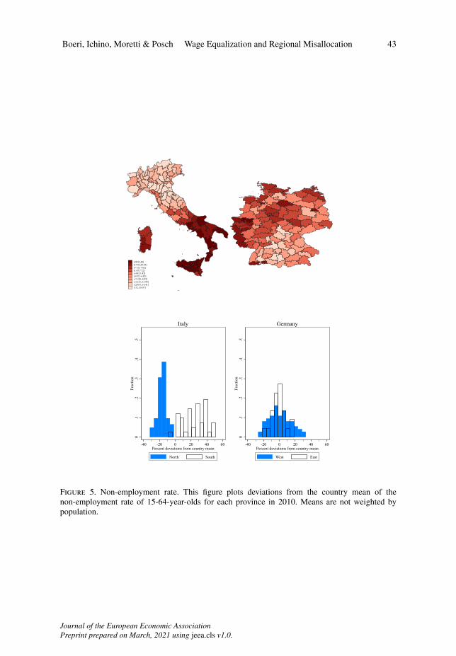
Boeri, Ichino, Moretti & Posch Wage Equalization and Regional Misallocation 43
(28.83,49](17.02,28.83](7.72,17.02](1.45,7.72](-4.45,1.45](-8.92,-4.45](-13.98,-8.92](-16.41,-13.98](-20.07,-16.41][-32,-20.07]
0.1
.2.3
.4.5
Frac
tion
-40 -20 0 20 40 60Percent deviations from country mean
North South
Italy
0.1
.2.3
.4.5
Frac
tion
-40 -20 0 20 40 60Percent deviations from country mean
West East
Germany
Figure 5. Non-employment rate. This �gure plots deviations from the country mean of thenon-employment rate of 15-64-year-olds for each province in 2010. Means are not weighted bypopulation.
Journal of the European Economic AssociationPreprint prepared on March, 2021 using jeea.cls v1.0.
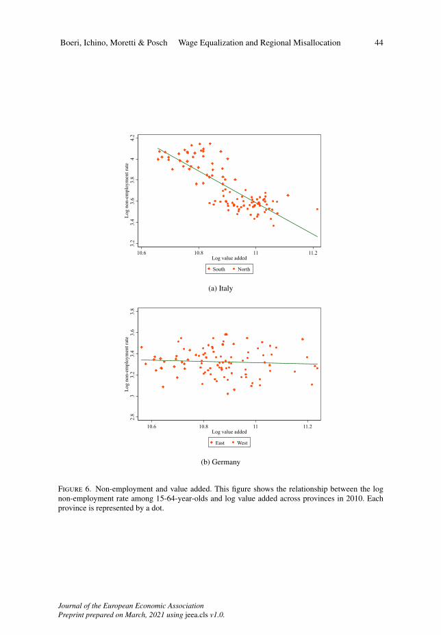
Boeri, Ichino, Moretti & Posch Wage Equalization and Regional Misallocation 44
3.2
3.4
3.6
3.8
44.
2Lo
g no
n-em
ploy
men
t rat
e
10.6 10.8 11 11.2Log value added
South North
(a) Italy
2.8
33.
23.
43.
63.
8Lo
g no
n-em
ploy
men
t rat
e
10.6 10.8 11 11.2Log value added
East West
(b) Germany
Figure 6. Non-employment and value added. This �gure shows the relationship between the lognon-employment rate among 15-64-year-olds and log value added across provinces in 2010. Eachprovince is represented by a dot.
Journal of the European Economic AssociationPreprint prepared on March, 2021 using jeea.cls v1.0.

Boeri, Ichino, Moretti & Posch Wage Equalization and Regional Misallocation 45
(16.16,68](11.15,16.16](7.44,11.15](4.1,7.44](-1.04,4.1](-4.52,-1.04](-7.99,-4.52](-11.8,-7.99](-17.83,-11.8][-32,-17.83]
0.1
.2.3
.4.5
Frac
tion
-80 -60 -40 -20 0 20 40 60 80Percent deviations from country mean
North South
Italy
0.1
.2.3
.4.5
Frac
tion
-80 -60 -40 -20 0 20 40 60 80Percent deviations from country mean
West East
Germany
Figure 7. Real wages. Deviations from the country mean of the mean conditional real wages ineuros (conditional nominal wages adjusted for consumer prices, as explained in Section 4) of eachprovince in 2010. Means are not weighted by population.
Journal of the European Economic AssociationPreprint prepared on March, 2021 using jeea.cls v1.0.

Boeri, Ichino, Moretti & Posch Wage Equalization and Regional Misallocation 46
1.7
1.9
2.1
2.3
2.5
2.7
Log
real
wag
e
10.6 10.8 11 11.2Log value added
South North
(a) Italy
44.
24.
44.
64.
85
Log
real
wag
e
10.6 10.8 11 11.2Log value added
East West
(b) Germany
Figure 8. Real wage and value added. This �gure shows the relationship between log meanconditional real wages (log conditional nominal wages adjusted for consumer prices, as explainedin Section 4) and log mean value added across provinces in 2010. Each province is represented by adot.
Journal of the European Economic AssociationPreprint prepared on March, 2021 using jeea.cls v1.0.