capital flows and financial stability: monetary policy and ... · capital flows and financial...
TRANSCRIPT
Capital Flows and Financial Stability:Monetary Policy and Macroprudential
Responses∗
D. Filiz UnsalInternational Monetary Fund
The resumption of capital flows to emerging-marketeconomies since mid-2009 has posed two sets of interrelatedchallenges for policymakers: (i) to prevent capital flows fromexacerbating overheating pressures and consequent inflation,and (ii) to minimize the risk that prolonged periods of easyfinancing conditions will undermine financial stability. Whileconventional monetary policy maintains its role in counteract-ing the former, there are doubts that it is sufficient to guardagainst the risks of financial instability. In this context, therehave been increased calls for the development of macropru-dential measures globally. Against this background, this paperanalyzes the interplay between monetary and macropruden-tial policies in an open-economy DSGE model. The key resultis that macroprudential measures can usefully complementmonetary policy under a financial shock that triggers capitalinflows. Even under the “optimal simple rules,” introducingmacroprudential measures improves welfare. Broad macropru-dential measures are shown to be more effective than those that
∗I am grateful to the editor Douglas Gale and an anonymous referee for valu-able comments and suggestions. I also thank the participants at the IJCB 4thFinancial Stability Conference on “Financial Crises: Causes, Consequences, andPolicy Options,” particularly Gianluca Benigno, Gianni De Nicolo, and RafaelPortillo. Roberto Cardarelli, Sonali Jain-Chandra, Nicolas Eyzaguirre, Jinill Kim,Nobuhiro Kiyotaki, Jaewoo Lee, and Steve Phillips; seminar participants in theIMF, in Korea University, and in the Central Bank of Turkey; and participantsat the KIEP-IMF Joint Conference also provided insightful comments and sug-gestions. The usual disclaimer applies. Author contact: Research Department,International Monetary Fund, 700 19th Street, N.W., Washington, DC 20431,USA; Tel: 202-623-0784; E-mail:[email protected].
233
234 International Journal of Central Banking March 2013
discriminate against foreign liabilities (macroprudential cap-ital controls). We also show that the exchange rate regimematters for the desirability of a macroprudential instrumentas a separate policy tool. Nevertheless, macroprudential meas-ures may not be as useful in helping economic stability underdifferent shocks. Therefore, shock-specific flexibility in theimplementation is desirable.
JEL Codes: E52, E61, F41.
1. Introduction
Unusually strong cyclical and policy differences between advancedand emerging economies, and a gradual shift in portfolio allocationtowards emerging markets, have led to capital flows into emerging-market economies since mid-2009. This rapid resumption of capi-tal inflows, which are large in historical context, has posed risks tomacroeconomic and financial stability. To address these risks, poli-cymakers have turned their attention to the use of macroprudentialmeasures, in addition to monetary policy.
Past experience has shown that macroeconomic stability is not asufficient condition for financial stability. For example, prior to thecrisis, financial imbalances built up in advanced economies despitestable growth and low inflation. Moreover, microprudential regula-tion and supervision, which focus on ensuring safety and soundnessof individual financial institutions, turned out to be inadequate, assystemwide risks could not be contained. Hence, a different approachbased on macroprudential supervision has started to be implementedin several emerging-market economies.
Macroprudential measures are defined as regulatory policies thataim to reduce systemic risks, ensure stability of the financial sys-tem as a whole against domestic and external shocks, and ensurethat it continues to function effectively (Bank for International Set-tlements 2010). During boom times, perceived risk declines, assetprices increase, and lending and leverage become mutually rein-forcing. The opposite happens during a bust phase: a vicious cyclecan arise between deleveraging, asset sales, and the real economy.This amplifying role of financial systems in propagating shocks—theso-called financial accelerator mechanism—implies procyclicality offinancial conditions. In principle, macroprudential measures could
Vol. 9 No. 1 Capital Flows and Financial Stability 235
address procyclicality of financial markets by making it harder toborrow during the boom times, and therefore make the subsequentreversal less dramatic, thus reducing the amplitude of the boom-bustcycles by design.
Both changes in policy interest rates and macroprudential meas-ures affect aggregate demand and supply as well as financial con-ditions in similar ways. On the one hand, monetary policy affectsasset prices and financial markets in general. Indeed, asset pricesare one channel through which monetary policy operates. On theother hand, macroprudential policies have macroeconomic spillovers,through cushioning or amplifying the economic cycle, or, for exam-ple, by directly affecting the provision of credit.
Nevertheless, the two instruments are not perfect substitutes andcan usefully complement each other, especially in the presence oflarge capital inflows that tend to increase vulnerabilities of the finan-cial system. First, the policy rate may be “too blunt” an instrument,as it impacts all lending activities regardless of whether they repre-sent a risk to stability of the economy.1 The interest rate increaserequired to deleverage specific sectors might be so large as to bringunduly large aggregate economic volatility. By contrast, macropru-dential regulations can be aimed specifically at markets in whichthe risk of financial stability is believed to be excessive.2 Second, ineconomies with open financial accounts, an increase in the interestrate might have only a limited impact on credit expansion if firmscan borrow at a lower rate abroad. Moreover, although monetarytransmission works well through the asset-price channel in “normal”times, in “abnormal” times sizable rapid changes in risk premiumscould offset or diminish the impact of policy rate changes on creditgrowth and asset prices (Kohn 2008; Bank of England 2009). Third,and perhaps more importantly, interest rate movements aiming toensure financial stability could be inconsistent with those requiredto achieve macroeconomic stability, and that discrepancy could riskde-anchoring inflation expectations (Borio and Lowe 2002; Mishkin
1See, among many others, Ostry et al. (2010).2The bluntness of the policy rate could also be its advantage over macropru-
dential measures, as it is difficult to circumvent a rise in borrowing costs broughtby policy rates in the same way as regulations can be avoided. See Bank forInternational Settlements (2010) and Ingves (2011).
236 International Journal of Central Banking March 2013
2007). For example, under an inflation-targeting framework, if theinflation outlook is consistent with the target, a response to asset-price fluctuations to maintain financial stability may damage thecredibility of the policy framework.
One initial question, however, is how a policy intervention to pri-vate borrowing decisions is justified in economic terms. This questioncan be answered in two main ways: first, by reference to negative exter-nalities that arise because agents do not internalize the effect of theirindividual decisions, which are distorted towards excessive borrow-ing, on financial instability; and, second, by reference to the potentialrole of macroprudential regulations in mitigating the standard Key-nesian impact of shocks—a decrease in aggregate demand and output,associated with a lower inflation—that cannot be fully offset by mone-tary and/or fiscal policies alone. There is a rapidly growing literatureon both fronts. On the first, Korinek (2009), Bianchi and Mendoza(2010), Jeanne andKorinek (2010), andBianchi (2011) focus on “over-borrowing” and consequent externalities. In these papers, regulationsinduce agents to internalize the externalities associated with theirdecisions and thereby increase macroeconomic stability. “Overbor-rowing,” however, is a model-specific feature. For example, Benignoet al. (2012) find that in normal times, “underborrowing” ismuchmorelikely to emerge than “overborrowing.”
This paper fits into the latter strand of research. Only recentlyhave several studies started analyzing interactions between mon-etary policy and macroprudential measures. Angeloni and Faia(2009), Kannan, Rabanal, and Scott (2009), N’Diaye (2009), andAngeloni, Faia, and Lo Duca (2010) incorporate macroprudentialinstruments into general equilibrium models where monetary policyhas a non-trivial role in stabilizing the economy after a shock. How-ever, all of these papers either feature a closed economy or do notexplicitly model the financial sector.
We analyze the trade-offs and complementarities between mon-etary and macroprudential policy rules (in the latter case, a rulethat responds to credit growth) in mitigating the impact of twoshocks that trigger capital inflows to the domestic economy: (i) afinancial shock (a shock to investors’ perception) and (ii) a shock toproductivity. This paper complements the existing literature in twoways. First, we add an open-economy dimension with a fully artic-ulated financial sector from the first principles. The model allows
Vol. 9 No. 1 Capital Flows and Financial Stability 237
a quantitative assessment of alternative monetary and macropru-dential responses to capital inflow surges. The open-economy fea-ture of the model also enables us to consider the incidence of theexchange rate regime on the relevance of macroprudential meas-ures. Further, we can assess the stabilization performance of macro-prudential measures that discriminate against foreign liabilities—macroprudential capital controls—versus broad macroprudentialmeasures, as entrepreneurs borrow from both domestic and foreignresources in the model. Second, the paper presents a welfare evalua-tion of alternative monetary and macroprudential policies. The liter-ature has so far focused on ad hoc specifications of a welfare measure,which could result in biased policy evaluations. We numerically com-pute welfare and derive welfare-maximizing policy options based ona second-order approximation of households’ utility function.
Our model features the financial accelerator mechanism devel-oped by Bernanke, Gertler, and Gilchrist (1999) and draws onelements of models by Gertler, Gilchrist, and Natalucci (2007),Kannan, Rabanal, and Scott (2009), and particularly Ozkan andUnsal (2010). The corporate sector plays a key role in the model—they decide the production and investment of capital, which is anasset and a way of accumulating wealth. In order to finance theirinvestments, corporations partially use internal funds. However, theyalso use external financing which is more costly, with the differencetermed “the default premium,” linking the terms of credit and bal-ance sheet conditions. Macroprudential policy rule (that respondsto nominal credit growth) entails higher costs for financial interme-diaries that are passed on to borrowers in the form of higher lendingrates. Therefore, in the model, macroprudential measures are definedas an additional “regulation premium” that adds to entrepreneurs’cost of borrowing.3 This setup captures the notion that such meas-ures make it harder for firms to borrow during boom times and hencemake the subsequent bust less dramatic.
In our framework, investors’ perception of risk declines under the(positive) financial shock, which provides easier credit conditions andhence triggers capital inflows. As financing costs decline, firms bor-row and invest more. Stronger demand for goods and higher asset
3In the case of macroprudential capital controls, the regulation premium onlyapplies to foreign borrowing.
238 International Journal of Central Banking March 2013
prices boost firms’ balance sheet and reduce the default premium fur-ther. Eventually, higher leverage brings a higher default premium,capital inflows slow, and financial conditions normalize. However,both monetary and macroprudential policies have a non-trivial rolein mitigating the impact of the shock.
We show that macroprudential policies help monetary policy sta-bilize the economy in the face of the financial shock. This is becausethey can offset the impact of the shock on entrepreneurs’ borrowingcosts without distorting consumption decisions by households. Wefind that even under the “optimal simple rules,” introducing macro-prudential measures is welfare improving. However, broad macro-prudential measures are more effective than macroprudential capitalcontrols, as the latter only bring a shift from foreign debt to domes-tic debt and hence affect the composition of entrepreneurs’ debt,rather than the total volume.
Our results also yield that the exchange rate regime matters forthe desirability of using a macroprudential instrument as a sepa-rate policy tool. Ceteris paribus, financial shocks have larger effectson inflation and output under the fixed exchange rate regime com-pared with the flexible exchange rate regime where the nominalexchange rate appreciation helps to limit the overheating and infla-tion pressures. In the absence of an independent policy tool underthe pegged exchange rate (and free capital mobility), macropruden-tial policies become the only tool available to deal with aggregatedemand stabilization.
Nevertheless, macroprudential measures may not be as usefulin helping economic stability under different shocks. Under a posi-tive productivity shock, for example, credit increases while inflationdecreases. Macroprudential policies that respond to credit growthchoke the desired expansion in credit brought by the endogenousmonetary policy easing. Hence, there is a trade-off between financialand macroeconomic stability objectives in the face of a productiv-ity shock, and macroprudential measures are not welfare improving.This implies that shock-specific flexibility in the implementation ofmacroprudential policies is desirable.
The remainder of the paper is organized as follows. Section 2sets out the structure of the model by describing household, firm,and entrepreneurial behavior with a special emphasis on financialintermediaries and macroprudential policies. Section 3 describes the
Vol. 9 No. 1 Capital Flows and Financial Stability 239
calibration, solution, and evaluation of the model. Section 4 presentsimpulse responses to a financial shock under alternative monetaryand macroprudential policies. Section 5 provides a welfare analy-sis of alternative policy responses. Section 6 discusses macroeco-nomic dynamics and a welfare evaluation under a productivity shock.Finally, section 7 provides the concluding remarks.
2. The Model
The world economy consists of two economies: a domestic economyand a foreign economy (rest of the world), each of which is inhabitedby infinitely lived households. The total measure of the world econ-omy is normalized to unity, with domestic and foreign having meas-ure n and (1−n), respectively. Following Galı and Monacelli (2005),Faia and Monacelli (2007), and De Paoli (2009), among many others,we assume that the domestic economy is very small in size relativeto the rest of the world to characterize an emerging, open-economycase.4
Three important modifications are introduced in this paper.First, we incorporate macroprudential measures into the monetarypolicy framework in a relatively traceable manner. Second, we allowentrepreneurs to borrow both from domestic and foreign resources.As will be explained later, this is a crucial departure in order to dif-ferentiate macroprudential measures that discriminate against for-eign liabilities (macroprudential capital controls) from more broadmacroprudential measures. Third, capital inflows to the domestic,open economy are modeled as a favorable change in the percep-tion of lenders. As they become “overoptimistic” about the domesticeconomy, financing conditions become easier. This is an intuitive andlikely realistic representation of what is going on in financial marketsduring sudden swings of capital across countries.
There are three types of firms in the model. Production firmsproduce a differentiated final consumption good using both capital
4Despite the fact that the domestic economy is very small in size relative tothe rest of the world, we choose to use a two-country model for greater realism,as it allows for some (small) feedback effects, which are general equilibrium innature. However, simulations for the specification where the size of the domesticeconomy is infinitely small yield qualitatively similar results.
240 International Journal of Central Banking March 2013
and labor as inputs. These firms engage in local currency pricing andface price adjustment costs. As a result, final goods’ prices are stickyin terms of the local exchange rate of the country in which they aresold. Importing firms that sell the goods produced in the foreigneconomy also have some market power and face adjustment costs inchanging prices. Price stickiness in export and import prices causesthe law of one price to fail such that exchange rate pass-throughis incomplete in the short run. Finally, there are competitive firmsthat combine investment with rented capital to produce unfinishedcapital goods that are then sold to entrepreneurs.
Entrepreneurs play a major role in the model. They producecapital, which is rented to firms, and finance their investment incapital through internal funds as well as external borrowing; how-ever, agency costs make the latter more expensive than the former.As monitoring the business activity of borrowers is a costly activity,lenders must be compensated by an external finance premium inaddition to the foreign or domestic interest rate. The magnitude ofthis premium varies with the leverage of the entrepreneurs, linkingthe terms of credit to balance sheet conditions.
In our framework, macroprudential measures entail an increasein financial intermediaries’ lending costs, which are then passed onto borrowers in the form of higher interest rates. We refer to theincreased lending rates brought by macroprudential measures as the“regulation premium” and maintain that it is positively linked tonominal credit growth. Macroprudential policy is therefore counter-cyclical by design: countervailing to the natural decline in perceivedrisk in good times and the subsequent rise in the perceived risk inbad times.
The model for the domestic economy is presented in this section,and we use a similar version of the model for the rest of the world.5
Although asymmetric in size, the domestic economy and the rest ofthe world share the same preferences, technology, and market struc-ture for consumption and capital goods. In what follows, variableswithout superscripts refer to the domestic economy, while variableswith a star indicate the rest-of-the-world variables unless indicatedotherwise.
5Appendices 1 and 2 present the model equations for the domestic small openeconomy and the rest of the world, respectively.
Vol. 9 No. 1 Capital Flows and Financial Stability 241
2.1 Households
A representative household is infinitely lived and seeks to maximize
E0
∞∑t=0
βt 11 − σ
(Ct − χ
1 + ϕH1+ϕ
t
)1−σ
, (1)
where Ct is a composite consumption index, Ht is hours of work,Et is the mathematical expectation conditional upon informationavailable at t, 0 < β < 1 is the representative consumer’s subjectivediscount factor, σ > 0 is the inverse of the intertemporal elasticityof substitution, χ > 0 is the utility weight of labor, and ϕ > 0 is theinverse elasticity of labor supply. Our specification for households’utility allows for Greenwood, Hercowitz, and Huffman (1988) (GHHhereafter) preferences over hours, which eliminates wealth effectsfrom labor supply.6
The composite consumption index, Ct, is given by
Ct =[(1 − α)
1γ C
(γ−1)/γH,t + (α)
1γ C
(γ−1)/γM,t
]γ/(γ−1), (2)
where γ > 0 is the elasticity of substitution between domestic andimported (foreign) goods, and 0 < α < 1 denotes the weight ofimported goods in the domestic consumption basket. This weight,α ≡ (1−n)υ, depends on (1−n), the relative size of the foreign econ-omy, and on υ, the degree of trade openness of the domestic econ-omy. CH,t and CM,t are constant elasticity of substitution indices ofconsumption of domestic and foreign goods, represented by
CH,t =[∫ 1
0CH,t(j)(λ−1)/λdj
]λ/(λ−1)
,
CM,t =[∫ 1
0CM,t(j)(λ−1)/λdj
]λ/(λ−1)
,
6Mendoza (1991), Correia, Neves, and Rebelo (1995), and Neumeyer and Perri(2005) show that specifying the utility function in line with GHH preferencesimproves the ability of the model to capture business-cycle dynamics. In section3.2, we analyze the performance of the model to reproduce some stylized factsfor a sample of emerging economies.
242 International Journal of Central Banking March 2013
where j ∈ [0, 1] indicates the goods varieties and λ > 1 is theelasticity of substitution among goods produced within a country.
The real exchange rate REXt is defined as REXt = StP∗t
Pt, where
St is the nominal exchange rate, domestic-currency price of foreigncurrency, and P ∗
t ≡ [∫ 10 P ∗
t (j)1−λdj]1/(1−λ) is the aggregate priceindex for foreign country’s consumption goods in foreign exchangerate. In contrast to most of the standard open-economy models,dynamics of P ∗
t are determined endogenously in our framework.Households in the domestic economy participate in domestic
and foreign financial markets: they lend to entrepreneurs in domes-tic currency, DD
t , and they borrow from international financialmarkets in foreign currency, DH
t , with a nominal interest rate ofit and i∗t ΨD,t, respectively. We follow the existing literature inassuming that households need to pay a premium, ΨD,t, given by
ΨD,t = ΨD
2 [exp( StDHt+1
PtGDPt− SDH
PGDP ) − 1]2 when they borrow from the
rest of the world.7 Households own all home production and theimporting firms and thus are recipients of profits, Πt. Other sourcesof income for the representative household are wages Wt, interestearnings in domestic currency, and new borrowing net of interestpayments on outstanding debts in foreign currency. Then, the rep-resentative household’s budget constraint in period t can be writtenas follows:
PtCt + DDt+1 + (1 + i∗t−1)ΨD,t−1StD
Ht
= WtHt + (1 + it−1)DDt + StD
Ht+1 + Πt. (3)
The representative household chooses sequences for {Ct, Ht,DD
t+1, DHt+1}∞
t=0 in order to maximize its expected lifetime utilityin (1) subject to the budget constraint in (3).
7We introduce this premium for households’ foreign borrowing to maintain thestationarity in the economy’s net foreign assets. In our calibration, the elasticityof the premium with respect to the debt is very close to zero (ΨD = 0.0075) sothat the dynamics of the model are not affected by the premium. See Schmitt-Grohe and Uribe (2003) for detailed discussions on other methods that inducestationarity in small open-economy models. Note that it would not be necessaryto introduce this premium when solving the model with a global solution, whichis not the case in this paper.
Vol. 9 No. 1 Capital Flows and Financial Stability 243
2.2 Firms
2.2.1 Production Firms
Each firm produces a differentiated good indexed by j ∈ [0, 1] usingthe production function:
Yt(j) = AtNt(j)1−ηKt(j)η, (4)
where At denotes total factor productivity common to all the pro-duction firms and it is assumed to follow an AR(1) process (ln(At) =ρA ln(At−1) + εA). Nt(j) is the labor input, which is a composite ofhousehold labor, Ht(j), and entrepreneurial labor, HE
t (j), defined asNt(j) = Ht(j)1−ΩHE
t (j)Ω. Kt(j) represents capital provided by theentrepreneur, as we explore in the following subsection. Assumingthat the price of each input is taken as given, the production firmsminimize their costs subject to (4).
Firms have some market power and they segment domestic andforeign markets with local currency pricing, where PH,t(j) andPX,t(j) denote price in the domestic market (in domestic currency)and price in the foreign market (in foreign currency). Firms also facequadratic menu costs in changing prices expressed in the units-of-consumption basket given by Ψi
2 ( Pi,t(j)Pi,t−1(j)
− 1)2 for different marketdestinations i = H, X. The presence of menu costs generates a grad-ual adjustment in the prices of goods in both markets, as suggestedby Rotemberg (1982). The combination of local-currency pricingand nominal price rigidities implies that fluctuations in the nom-inal exchange rate have a smaller impact on export prices so thatthe exchange rate pass-through to export prices is incomplete in theshort run.
As firms are owned by domestic households, the individual firmmaximizes its expected value of future profits using the household’sintertemporal rate of substitution in consumption, given by βtUc,t.The objective function of firm j can thus be written as
Eo
∞∑t=0
βtUc,t
Pt
[PH,t(j)YH,t(j) + StPX,t(j)YX,t(j) − MCtYt(j)
−Pt
∑i=H,X
Ψi
2
(Pi,t(j)
Pi,t−1(j)− 1
)2⎤⎦ , (5)
244 International Journal of Central Banking March 2013
where YH,t(j) and YX,t(j) represent domestic and foreign demandfor the domestically produced good j. We assume that different vari-eties have the same elasticities in both markets, so that the demandfor good j can be written as
Yi,t(j) =(
Pi,t(j)Pi,t
)−λ
Yi,t, for i = H, X, (6)
where PH,t is the aggregate price index for goods sold in the domes-tic market, as is defined earlier, and PX,t is the export price indexgiven by PX,t ≡ [
∫ 10 PX,t(j)1−λdj]1/(1−λ).
2.2.2 Importing Firms
There is a set of monopolistically competitive importing firms,owned by domestic households, that buy foreign goods at prices P ∗
X,t
(in local currency) and then sell them to the domestic market. Theyare also subject to a price adjustment cost with ΨM � 0, the cost-of-price-adjustment parameter, analogous to the production firms. Thisimplies that there is some delay between exchange rate changes andthe import price adjustments so that the short-run exchange ratepass-through to import prices is also incomplete.
2.2.3 Unfinished-Capital-Producing Firms
Let It denote aggregate investment in period t, which is composedof domestic and final goods:
It =[α
1γ I
(γ−1)/γH,t + (1 − α)
1γ I
(γ−1)/γM,t
]γ/(γ−1), (7)
where the domestic and imported investment goods’ prices areassumed to be the same as the domestic and import consumer goods’prices, PH,t and PM,t. The new capital stock requires the same com-bination of domestic and foreign goods so that the nominal price ofa unit of investment equals the price level, Pt.
Competitive firms use investment, It, as an input, and combineit with rented capital Kt to produce unfinished capital goods. Weassume that the marginal return to investment in terms of capitalgoods is decreasing in the amount of investment undertaken (relative
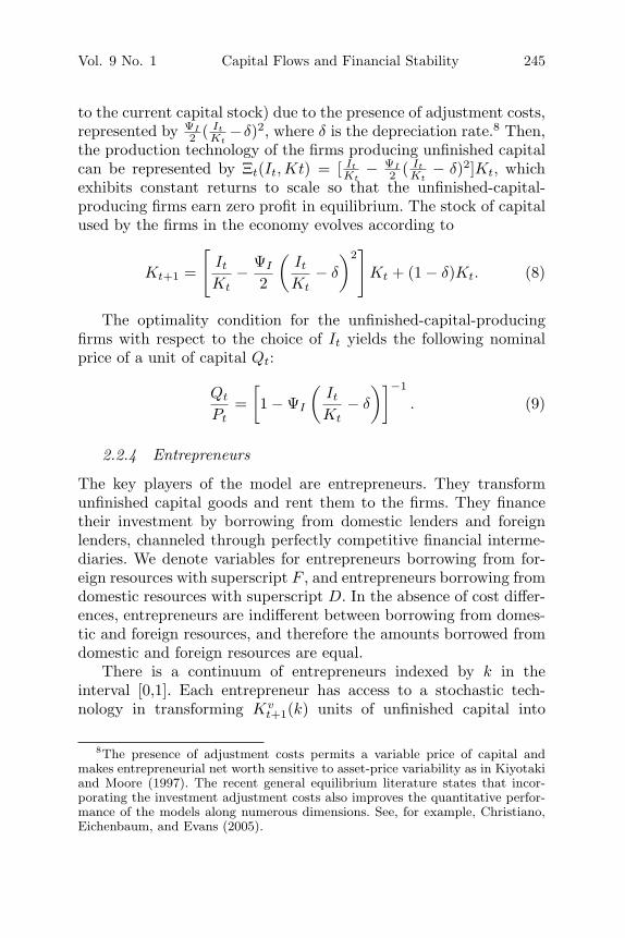
Vol. 9 No. 1 Capital Flows and Financial Stability 245
to the current capital stock) due to the presence of adjustment costs,represented by ΨI
2 ( It
Kt−δ)2, where δ is the depreciation rate.8 Then,
the production technology of the firms producing unfinished capitalcan be represented by Ξt(It, Kt) = [ It
Kt− ΨI
2 ( It
Kt− δ)2]Kt, which
exhibits constant returns to scale so that the unfinished-capital-producing firms earn zero profit in equilibrium. The stock of capitalused by the firms in the economy evolves according to
Kt+1 =
[It
Kt− ΨI
2
(It
Kt− δ
)2]
Kt + (1 − δ)Kt. (8)
The optimality condition for the unfinished-capital-producingfirms with respect to the choice of It yields the following nominalprice of a unit of capital Qt:
Qt
Pt=
[1 − ΨI
(It
Kt− δ
)]−1
. (9)
2.2.4 Entrepreneurs
The key players of the model are entrepreneurs. They transformunfinished capital goods and rent them to the firms. They financetheir investment by borrowing from domestic lenders and foreignlenders, channeled through perfectly competitive financial interme-diaries. We denote variables for entrepreneurs borrowing from for-eign resources with superscript F , and entrepreneurs borrowing fromdomestic resources with superscript D. In the absence of cost differ-ences, entrepreneurs are indifferent between borrowing from domes-tic and foreign resources, and therefore the amounts borrowed fromdomestic and foreign resources are equal.
There is a continuum of entrepreneurs indexed by k in theinterval [0,1]. Each entrepreneur has access to a stochastic tech-nology in transforming Kv
t+1(k) units of unfinished capital into
8The presence of adjustment costs permits a variable price of capital andmakes entrepreneurial net worth sensitive to asset-price variability as in Kiyotakiand Moore (1997). The recent general equilibrium literature states that incor-porating the investment adjustment costs also improves the quantitative perfor-mance of the models along numerous dimensions. See, for example, Christiano,Eichenbaum, and Evans (2005).
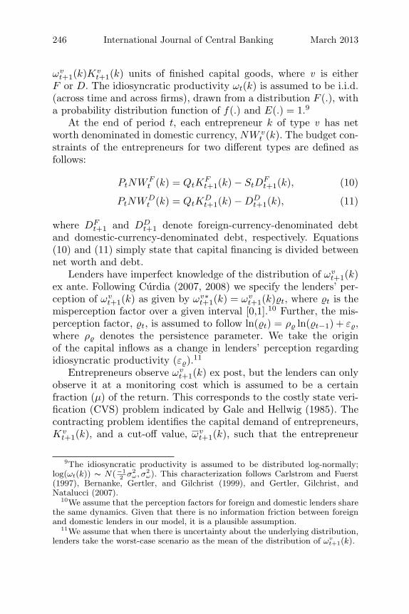
246 International Journal of Central Banking March 2013
ωvt+1(k)Kv
t+1(k) units of finished capital goods, where v is eitherF or D. The idiosyncratic productivity ωt(k) is assumed to be i.i.d.(across time and across firms), drawn from a distribution F (.), witha probability distribution function of f(.) and E(.) = 1.9
At the end of period t, each entrepreneur k of type v has networth denominated in domestic currency, NW v
t (k). The budget con-straints of the entrepreneurs for two different types are defined asfollows:
PtNWFt (k) = QtK
Ft+1(k) − StD
Ft+1(k), (10)
PtNWDt (k) = QtK
Dt+1(k) − DD
t+1(k), (11)
where DFt+1 and DD
t+1 denote foreign-currency-denominated debtand domestic-currency-denominated debt, respectively. Equations(10) and (11) simply state that capital financing is divided betweennet worth and debt.
Lenders have imperfect knowledge of the distribution of ωvt+1(k)
ex ante. Following Curdia (2007, 2008) we specify the lenders’ per-ception of ωv
t+1(k) as given by ωv∗t+1(k) = ωv
t+1(k)�t, where �t is themisperception factor over a given interval [0,1].10 Further, the mis-perception factor, �t, is assumed to follow ln(�t) = ρ� ln(�t−1) + ε�,where ρ� denotes the persistence parameter. We take the originof the capital inflows as a change in lenders’ perception regardingidiosyncratic productivity (ε�).11
Entrepreneurs observe ωvt+1(k) ex post, but the lenders can only
observe it at a monitoring cost which is assumed to be a certainfraction (μ) of the return. This corresponds to the costly state veri-fication (CVS) problem indicated by Gale and Hellwig (1985). Thecontracting problem identifies the capital demand of entrepreneurs,Kv
t+1(k), and a cut-off value, ωvt+1(k), such that the entrepreneur
9The idiosyncratic productivity is assumed to be distributed log-normally;log(ωt(k)) ∼ N(−1
2 σ2ω, σ2
ω). This characterization follows Carlstrom and Fuerst(1997), Bernanke, Gertler, and Gilchrist (1999), and Gertler, Gilchrist, andNatalucci (2007).
10We assume that the perception factors for foreign and domestic lenders sharethe same dynamics. Given that there is no information friction between foreignand domestic lenders in our model, it is a plausible assumption.
11We assume that when there is uncertainty about the underlying distribution,lenders take the worst-case scenario as the mean of the distribution of ωv
t+1(k).
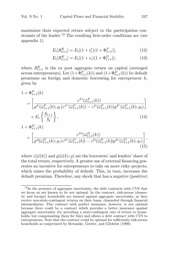
Vol. 9 No. 1 Capital Flows and Financial Stability 247
maximizes their expected return subject to the participation con-straints of the lender.12 The resulting first-order conditions are (seeappendix 1)
Et[RKt+1] = Et[(1 + i∗t )(1 + ΦF
t+1)], (12)
Et[RKt+1] = Et[(1 + it)(1 + ΦD
t+1)], (13)
where RKt+1 is the ex post aggregate return on capital (averaged
across entrepreneurs). Let (1+ΦFt+1(k)) and (1+ΦD
t+1(k)) be defaultpremiums on foreign and domestic borrowing for entrepreneur k,given by
1 + ΦFt+1(k)
=[
zF ′(ωFt+1(k))
gF (ωFt+1(k); �t)zF ′(ωF
t+1(k)) − zF (ωFt+1(k))gF ′(ωF
t+1(k); �t)
]
× Et
{St+1
St
}, (14)
1 + ΦDt+1(k)
=[
zD′(ωDt+1(k))
gD(ωDt+1(k); �t)zD′(ωD
t+1(k)) − zD(ωDt+1(k))gD′(ωD
t+1(k); �t)
],
(15)
where z(ω(k)) and g(ω(k); �) are the borrowers’ and lenders’ share ofthe total return, respectively. A greater use of external financing gen-erates an incentive for entrepreneurs to take on more risky projects,which raises the probability of default. This, in turn, increases thedefault premium. Therefore, any shock that has a negative (positive)
12In the presence of aggregate uncertainty, the debt contracts with CVS thatwe focus on are known to be not optimal. In the contract, risk-averse (domes-tic and foreign) households are insured against aggregate uncertainty, as theyreceive non-state-contingent returns on their loans, channeled through financialintermediaries. This contract with perfect insurance, however, is not optimalbecause there could be a contract which provides a better insurance againstaggregate uncertainty (by providing a state-contingent rate of return to house-holds, but compensating them for this) and allows a debt contract with CVS toentrepreneurs. Note that the contract could be optimal for sufficiently risk-aversehouseholds as conjectured by Bernanke, Gertler, and Gilchrist (1999).
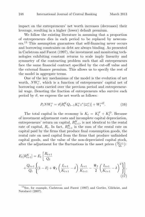
248 International Journal of Central Banking March 2013
impact on the entrepreneurs’ net worth increases (decreases) theirleverage, resulting in a higher (lower) default premium.
We follow the existing literature in assuming that a proportionof entrepreneurs dies in each period to be replaced by newcom-ers.13 This assumption guarantees that self-financing never occursand borrowing constraints on debt are always binding. As presentedin Carlstrom and Fuerst (1997), the investment and monitoring tech-nologies exhibiting constant returns to scale imply linearity andsymmetry of the contracting problem such that all entrepreneursface the same financial contract specified by the cut-off value andthe external finance premium. This allows us to specify the rest ofthe model in aggregate terms.
One of the key mechanisms of the model is the evolution of networth, NW v
t , which is a function of entrepreneurs’ capital net ofborrowing costs carried over the previous period and entrepreneur-ial wage. Denoting the fraction of entrepreneurs who survive eachperiod by ϑ, we express the net worth as follows:
PtNW vt = ϑ[RK
t Qt−1Kvt zv (ωv
t )] + W vEt . (16)
The total capital in the economy is Kt = KFt + KD
t . Becauseof investment adjustment costs and incomplete capital depreciation,entrepreneurs’ return on capital, RK
t+1, is not identical to the rentalrate of capital, Rt. In fact, RK
t+1 is the sum of the rental rate oncapital paid by the firms that produce final consumption goods, therental rate on used capital from the firms that produce unfinishedcapital goods, and the value of the non-depreciated capital stock,after the adjustment for the fluctuations in the asset prices (Qt+1
Qt):
Et[RKt+1] = Et
[Rt+1
Qt
+Qt+1
Qt
{(1 − δ) + ΨI
(It+1
Kt+1− δ
)It+1
Kt+1− ΨI
2
(It+1
Kt+1− δ
)2}]
.
(17)
13See, for example, Carlstrom and Fuerst (1997) and Gertler, Gilchrist, andNatalucci (2007).
Vol. 9 No. 1 Capital Flows and Financial Stability 249
2.4 Financial Intermediaries and Macroprudential Policy
There exists a continuum of perfectly competitive financial interme-diaries which collect deposits from households and loan the moneyout to entrepreneurs in each period. They also receive capital inflowsfrom the foreign economy in the form of loans to domestic entre-preneurs. The sum of deposits and capital inflows makes up thetotal supply of loanable funds. The zero-profit condition on finan-cial intermediaries implies that the lending rates are just equal toEt[(1 + i∗t )(1 + ΦF
t+1)] and Et[(1 + it)(1 + ΦDt+1)] in the absence of
macroprudential measures.Either in the form of capital requirements or loan-to-value ceil-
ing, or some other type, macroprudential policy entails higher costsfor financial intermediaries. Rather than deriving the impact of aparticular type of macroprudential measure on the borrowing cost,we follow Kannan, Rabanal, and Scott (2009) and focus on a genericcase where macroprudential measures lead to an additional cost tofinancial intermediaries. These costs are then reflected to borrowersin the form of higher interest rates.14 The increase in the lendingrates brought by (broad) macroprudential measures is called the“regulation premium” and is a function of nominal credit growth.15
In the presence of macroprudential regulations, the spreadbetween lending rate and policy rate is affected by both the defaultpremium and the regulation premium. Hence, the lending costs forforeign borrowing and domestic borrowing, equations (12) and (13),become
Et[RKt+1] = Et[(1 + i∗t )(1 + ΦF
t+1)(1 + RPt)], (18)
Et[RKt+1] = Et[(1 + it)(1 + ΦD
t+1)(1 + RPt)], (19)
14By adopting a more elaborate banking sector, Angeloni and Faia (2009),Angeloni, Faia, and Lo Duca (2010), and Gertler and Karadi (2011) show thatmacroprudential measures in fact lead to an increase in the cost of borrowing.In an open-economy framework, following a similar approach would make themodel hardly traceable. Therefore, we use a simpler specification here and leaveanalysis of frictions related to financial intermediaries for future work.
15See Borgy, Clerc, and Renne (2009), Borio and Drehman (2009), andGerdesmeier, Roffia, and Reimers (2009) for discussions on the potential roleof nominal credit growth in a regulation tool.
250 International Journal of Central Banking March 2013
where RPt is the regulation premium, which is defined in the baselinecase as a function of the aggregate nominal credit growth:
RPt = Ψ(
Dt
Dt−1− 1
), (20)
where Dt = StDFt +DD
t . In this definition of broad macroprudentialpolicy, it is implicit that the policy objective is defined in terms ofaggregate credit activity. In the case of macroprudential measuresthat discriminate against foreign liabilities (macroprudential capitalcontrols), the regulation premium only applies to foreign borrow-ing (18) and the macroprudential policy instrument (RPt) is definedonly in terms of nominal foreign credit growth.
2.4.1 Monetary Policy
In the baseline calibration, we adopt a standard formulation for thestructure of monetary policymaking. We assume that the interestrate rule is of the following form:
1 + it = [(1 + i)(πt)επ(Yt/Y )εY ][1 + it−1]1−, (21)
with {επ} ∈ (1,∞], {εY } ∈ (0,∞], and � ∈ [0, 1]. In (21) � is theinterest rate smoothing parameter, i and Y denote the steady-statelevel of nominal interest rate and output, and πt is the CPI inflation.We start with an initial set of values for επ, εY , and � in the calibra-tion. In the optimal simple rules, however, we numerically computethe optimal values of επ and εY (as well as the macroprudentialrule coefficient Ψ) that maximize the welfare measure derived fromhouseholds’ utility function (further discussion is presented below).
3. Calibration, Solution Strategy, and Model Evaluation
In this section we first describe the calibration of the model and themodel solution. We then discuss the model’s ability to fit the datafor typical emerging, open economies.
3.1 Calibration and Solution Strategy
The parameters for consumption, production, and entrepreneurialsectors are assumed to be identical for the domestic economy and
Vol. 9 No. 1 Capital Flows and Financial Stability 251
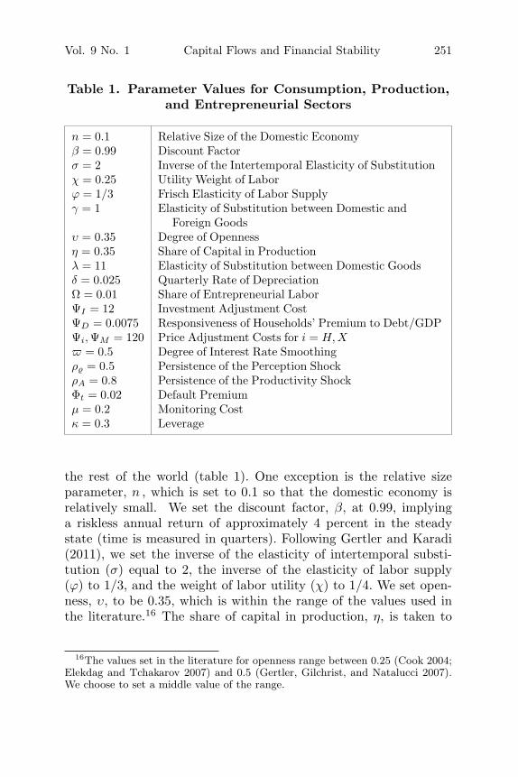
Table 1. Parameter Values for Consumption, Production,and Entrepreneurial Sectors
n = 0.1 Relative Size of the Domestic Economyβ = 0.99 Discount Factorσ = 2 Inverse of the Intertemporal Elasticity of Substitutionχ = 0.25 Utility Weight of Laborϕ = 1/3 Frisch Elasticity of Labor Supplyγ = 1 Elasticity of Substitution between Domestic and
Foreign Goodsυ = 0.35 Degree of Opennessη = 0.35 Share of Capital in Productionλ = 11 Elasticity of Substitution between Domestic Goodsδ = 0.025 Quarterly Rate of DepreciationΩ = 0.01 Share of Entrepreneurial LaborΨI = 12 Investment Adjustment CostΨD = 0.0075 Responsiveness of Households’ Premium to Debt/GDPΨi, ΨM = 120 Price Adjustment Costs for i = H, X� = 0.5 Degree of Interest Rate Smoothingρ� = 0.5 Persistence of the Perception ShockρA = 0.8 Persistence of the Productivity ShockΦt = 0.02 Default Premiumμ = 0.2 Monitoring Costκ = 0.3 Leverage
the rest of the world (table 1). One exception is the relative sizeparameter, n , which is set to 0.1 so that the domestic economy isrelatively small. We set the discount factor, β, at 0.99, implyinga riskless annual return of approximately 4 percent in the steadystate (time is measured in quarters). Following Gertler and Karadi(2011), we set the inverse of the elasticity of intertemporal substi-tution (σ) equal to 2, the inverse of the elasticity of labor supply(ϕ) to 1/3, and the weight of labor utility (χ) to 1/4. We set open-ness, υ, to be 0.35, which is within the range of the values used inthe literature.16 The share of capital in production, η, is taken to
16The values set in the literature for openness range between 0.25 (Cook 2004;Elekdag and Tchakarov 2007) and 0.5 (Gertler, Gilchrist, and Natalucci 2007).We choose to set a middle value of the range.
252 International Journal of Central Banking March 2013
be 0.35, consistent with other studies.17 Following Devereux, Lane,and Xu (2006), the elasticity of substitution between differentiatedgoods of the same origin, λ, is taken to be 11, implying a flexible-price equilibrium markup of 1.1. Price adjustment cost is assumedto be 120 for all sectors. The quarterly depreciation rate (δ) is 0.025.Similar to Gertler, Gilchrist, and Natalucci (2007), we set the shareof entrepreneurs’ labor, Ω, at 0.01, implying that 1 percent of thetotal wage bill goes to the entrepreneurs. We set the steady-stateleverage ratio and the value of the quarterly default premium at 0.3and 200 basis points, respectively, reflecting the historical averageof emerging-market economies within the last decade.18 The moni-toring cost parameter, μ, is taken as 0.2 as in Devereux, Lane, andXu (2006). The degree of interest rate smoothing parameter (�) ischosen as 0.5. ρ� is assumed to be 0.5, so that it takes nine quartersfor the shock to die away.19
We analyze the macroeconomic impact of an unanticipated (tem-porary) favorable shock to (both domestic and foreign) investors’perception regarding productivity of entrepreneurs—an “optimism”shock. In particular, we give a 1 percent positive shock to the (log of)misperception factor (ln(�t)).20 We present responses of the econ-omy under several monetary and macroprudential policy options,namely (i) Taylor rule, (ii) Taylor rule with broad macropruden-tial policy, (iii) Taylor rule with macroprudential capital controls,(iv) fixed exchange rate regime, (v) fixed exchange rate regimewith broad macroprudential policy, and (vi) fixed exchange rateregime with macroprudential capital controls. Table 2 represents the
17See, for example, Cespedes, Chang, and Velasco (2004) and Elekdag andTchakarov (2007).
18This is the average number for emerging Americas, emerging Asia, and emerg-ing Europe between 2000 and 2010. Worldscope data (debt as a percentage ofassets—data item WS 08236) is used for the leverage ratio. The default pre-mium is calculated as the difference between the lending and the policy rate foremerging-market countries, where available, using data from Haver Analytics forthe same time period. Variations in these parameters do not affect our resultsqualitatively.
19We carry out several sensitivity analyses in order to assess robustness of ourresults under the benchmark calibration. To conserve space, we do not reportthese results, but they are available upon request.
20The optimism shock brings about a 1.25 and 2 percent decline in domesticand foreign default premiums, respectively, under the baseline calibration, and asurge in capital inflows by about 1 percent of output.
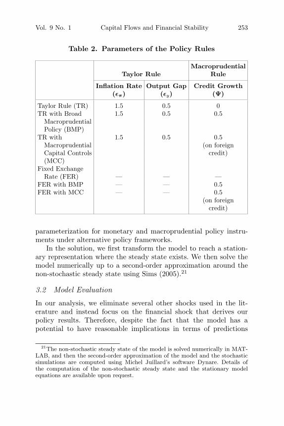
Vol. 9 No. 1 Capital Flows and Financial Stability 253
Table 2. Parameters of the Policy Rules
MacroprudentialTaylor Rule Rule
Inflation Rate Output Gap Credit Growth(επ) (εy) (Ψ)
Taylor Rule (TR) 1.5 0.5 0TR with Broad 1.5 0.5 0.5
MacroprudentialPolicy (BMP)
TR with 1.5 0.5 0.5Macroprudential (on foreignCapital Controls credit)(MCC)
Fixed ExchangeRate (FER) — — —
FER with BMP — — 0.5FER with MCC — — 0.5
(on foreigncredit)
parameterization for monetary and macroprudential policy instru-ments under alternative policy frameworks.
In the solution, we first transform the model to reach a station-ary representation where the steady state exists. We then solve themodel numerically up to a second-order approximation around thenon-stochastic steady state using Sims (2005).21
3.2 Model Evaluation
In our analysis, we eliminate several other shocks used in the lit-erature and instead focus on the financial shock that derives ourpolicy results. Therefore, despite the fact that the model has apotential to have reasonable implications in terms of predictions
21The non-stochastic steady state of the model is solved numerically in MAT-LAB, and then the second-order approximation of the model and the stochasticsimulations are computed using Michel Juillard’s software Dynare. Details ofthe computation of the non-stochastic steady state and the stationary modelequations are available upon request.
254 International Journal of Central Banking March 2013
of macroeconomic variables, we cannot expect that the model willmatch in all dimensions the data. However, to generate confidencein the model’s ability to correctly capture dynamics, and on the pro-posed calibration of the parameters’ values, we compare movementsand co-movements of some key variables.
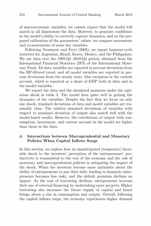
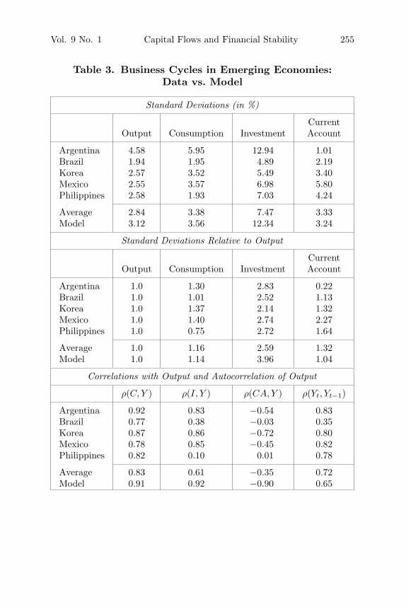
Following Neumeyer and Perri (2005), we report business-cyclestatistics for Argentina, Brazil, Korea, Mexico, and the Philippines.We use data over the 1995:Q1–2010:Q4 period, obtained from theInternational Financial Statistics (IFS) of the International Mone-tary Fund. All data variables are reported in percent deviations fromthe HP-filtered trend, and all model variables are reported in per-cent deviations from the steady state. One exception is the currentaccount, which is reported as a share of GDP both in data and inthe model variables.
We report the data and the simulated moments under the opti-mism shock in table 3. The model does quite well in getting thedynamics of the variables. Despite the fact that we focus on onlyone shock, standard deviations of data and model variables are rea-sonably close. The relative standard deviations of variables withrespect to standard deviation of output also match well with themodel-based results. However, the correlations of output with con-sumption, investment, and current account in the model are higherthan those in the data.
4. Interactions between Macroprudential and MonetaryPolicies When Capital Inflows Surge
In this section, we explore how an unanticipated (temporary) favor-able shock to the investors’ perception of the entrepreneurs’ pro-ductivity is transmitted to the rest of the economy and the role ofmonetary and macroprudential policies in mitigating the impact ofthe shock. When the investors become more optimistic about theability of entrepreneurs to pay their debt, lending to domestic entre-preneurs becomes less risky, and the default premium declines onimpact. As the cost of borrowing declines, entrepreneurs increasetheir use of external financing by undertaking more projects. Higherborrowing also increases the future supply of capital and hencebrings about a rise in consumption and output. Overall, followingthe capital inflows surge, the economy experiences higher demand
Vol. 9 No. 1 Capital Flows and Financial Stability 255
Table 3. Business Cycles in Emerging Economies:Data vs. Model
Standard Deviations (in %)
CurrentOutput Consumption Investment Account
Argentina 4.58 5.95 12.94 1.01Brazil 1.94 1.95 4.89 2.19Korea 2.57 3.52 5.49 3.40Mexico 2.55 3.57 6.98 5.80Philippines 2.58 1.93 7.03 4.24
Average 2.84 3.38 7.47 3.33Model 3.12 3.56 12.34 3.24
Standard Deviations Relative to Output
CurrentOutput Consumption Investment Account
Argentina 1.0 1.30 2.83 0.22Brazil 1.0 1.01 2.52 1.13Korea 1.0 1.37 2.14 1.32Mexico 1.0 1.40 2.74 2.27Philippines 1.0 0.75 2.72 1.64
Average 1.0 1.16 2.59 1.32Model 1.0 1.14 3.96 1.04
Correlations with Output and Autocorrelation of Output
ρ(C, Y ) ρ(I, Y ) ρ(CA, Y ) ρ(Yt, Yt−1)
Argentina 0.92 0.83 −0.54 0.83Brazil 0.77 0.38 −0.03 0.35Korea 0.87 0.86 −0.72 0.80Mexico 0.78 0.85 −0.45 0.82Philippines 0.82 0.10 0.01 0.78
Average 0.83 0.61 −0.35 0.72Model 0.91 0.92 −0.90 0.65
256 International Journal of Central Banking March 2013
and inflation pressures, along with a credit growth boom.22 In thatcase, macroprudential policies which directly counteract easing inthe lending standards might mitigate the impact of the shock andtherefore improve macroeconomic and financial stability.
The exchange rate regime is an important determinant of howthe shocks transmit to the rest of the economy and the role of macro-prudential policies. The surge in capital inflows increases the sup-ply of foreign debt and demand for domestic assets, and exchangerate appreciates under the Taylor-type monetary policy rule. Theexchange rate appreciation reduces the impact of the shock throughmainly two channels. First, the appreciation brings a downward pres-sure on the CPI-based inflation through lower imported good prices.Second, the rest of the world’s demand for domestic goods decreasesas they become relatively more expensive. Moreover, importsincrease on account of income and exchange rate effects followingthe shock. Hence, the trade balance deteriorates, which reduces theoutput response of the shock.23 Under a fixed exchange rate regime,however, the adjustment on the external balance has to rely on anincrease in the domestic price level. Interest rates remain low, andthe responses of consumption, output, and inflation are more pro-nounced. Given the absence of an independent policy tool, the useof macroprudential policies can provide a mechanism for promotingmacroeconomic stability under the fixed exchange rate regime.
We first focus on the standard Taylor rule and the Taylor rulewith broad macroprudential policy. Next, we consider broad macro-prudential policy and macroprudential measures on foreign liabil-ities (macroprudential capital controls). Then, we analyze broadand foreign liability-specific macroprudential policies under thefixed exchange rate regime. Note that we just present a posi-tive description of the dynamics under alternative monetary andmacroprudential policies in this section, without any judgment in
22These are in line with the experience of several emerging-market countries incapital inflows episodes (Cardarelli, Elekdag, and Kose 2010).
23The exchange rate appreciation has also an indirect impact on inflationand output through its impact on debt dynamics. The unanticipated changein the exchange rate creates a (positive) balance sheet effect for the foreign-currency-borrowing entrepreneurs through a decline in the real debt burden.This exacerbates the effects of the shock on debt dynamics, and hence on outputand inflation. However, this indirect impact is relatively small under reasonableparameterizations in our model.
Vol. 9 No. 1 Capital Flows and Financial Stability 257
terms of optimality of one policy over another. We leave the norma-tive policy analysis to section 5.
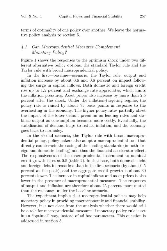
4.1 Can Macroprudential Measures ComplementMonetary Policy?
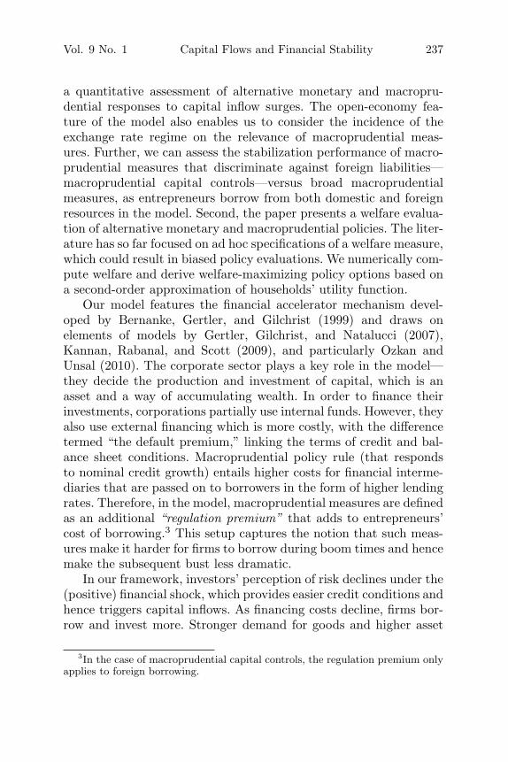
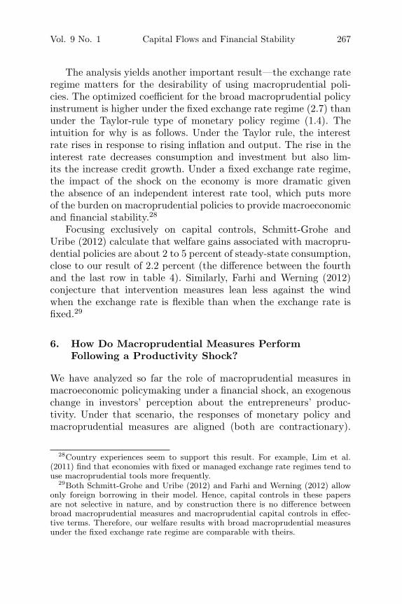
Figure 1 shows the responses to the optimism shock under two dif-ferent alternative policy options: the standard Taylor rule and theTaylor rule with broad macroprudential policy.
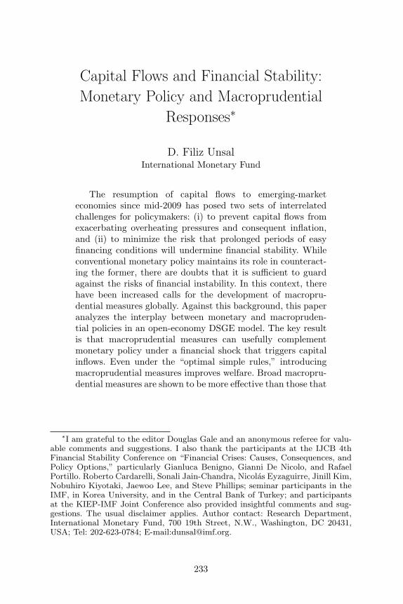
In the first—baseline—scenario, the Taylor rule, output andinflation increase by about 0.6 and 0.8 percent on impact follow-ing the surge in capital inflows. Both domestic and foreign creditrise up to 1.5 percent and exchange rate appreciates, which limitsthe inflation pressures. Asset prices also increase by more than 2.5percent after the shock. Under the inflation-targeting regime, thepolicy rate is raised by about 75 basis points in response to theoverheating in the economy. The higher policy rates partially offsetthe impact of the lower default premium on lending rates and sta-bilize output as consumption becomes more costly. Eventually, thestabilization of demand helps to reduce inflation, and the economygoes back to normalcy.
In the second scenario, the Taylor rule with broad macropru-dential policy, policymakers also adopt a macroprudential tool thatdirectly counteracts the easing of the lending standards (in both for-eign and domestic lending) and thus the financial accelerator effect.The responsiveness of the macroprudential instrument to nominalcredit growth is set at 0.5 (table 2). In that case, both domestic debtand foreign debt increase less than in the first scenario (by about 0.5percent at the peak), and the aggregate credit growth is about 30percent slower. The increase in capital inflows and asset prices is alsolower in the presence of macroprudential measures. The responsesof output and inflation are therefore about 25 percent more mutedthan the responses under the baseline scenario.
The experiment implies that macroprudential policies may helpmonetary policy in providing macroeconomic and financial stability.However, it is not clear from the analysis whether there would stillbe a role for macroprudential measures if monetary policy rule is setin an “optimal” way, instead of ad hoc parameters. This question isaddressed in section 5.
258 International Journal of Central Banking March 2013
Figure 1. A Positive Financial Shock: Taylor Rule andBroad Macroprudential Policy (percent deviations from
the steady state)
Notes: The figures show the impact of a 1 percent positive shock to the per-ception of investors regarding the productivity of domestic entrepreneurs. Thevariables are presented as log-deviations from the steady state (except for interestrate), multiplied by 100 to have an interpretation of percentage deviations.
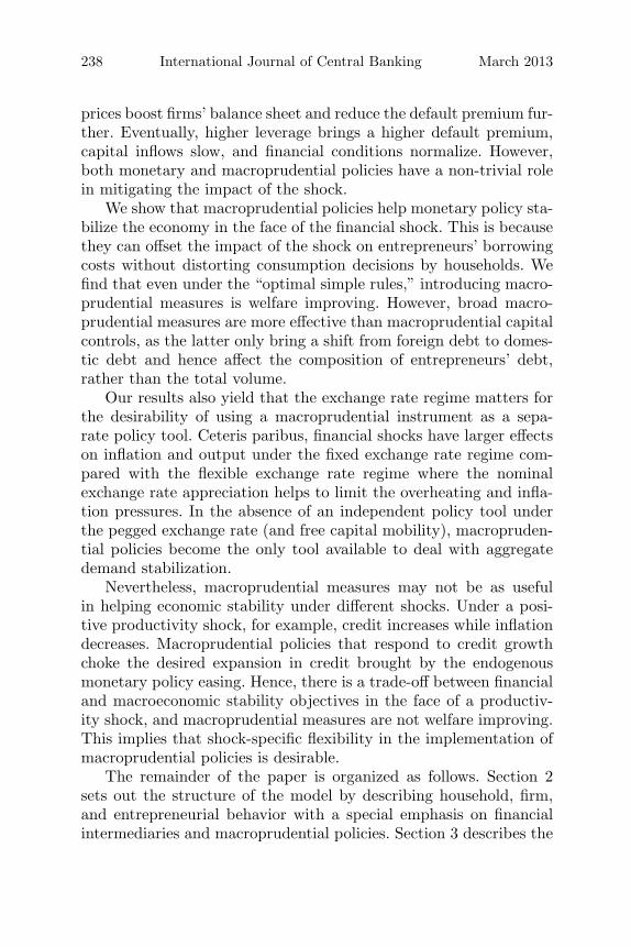
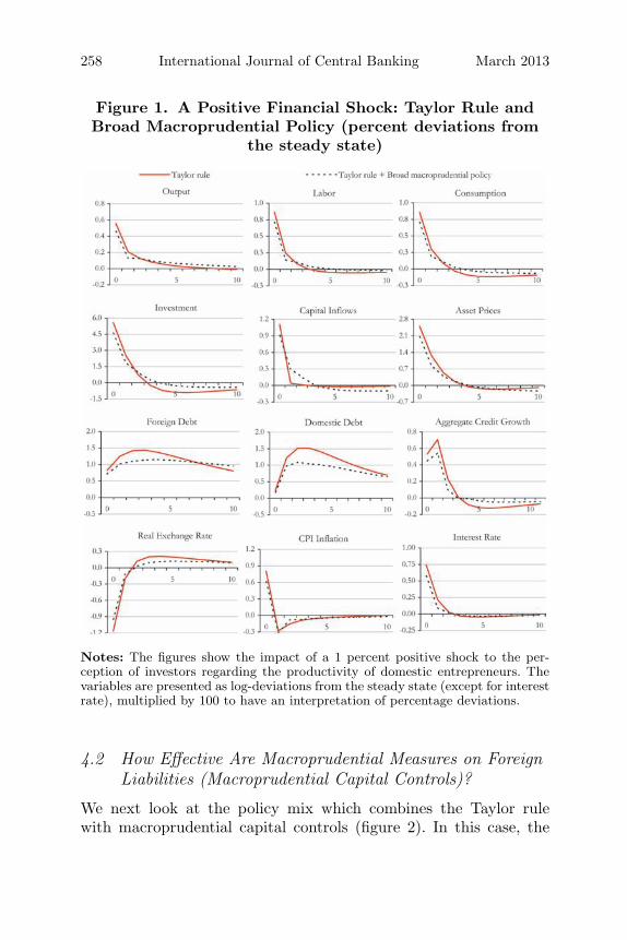
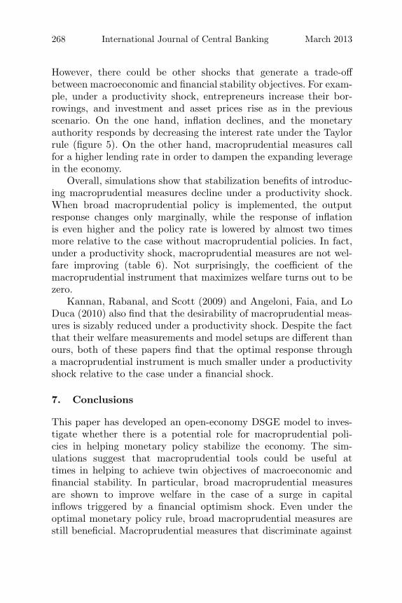
4.2 How Effective Are Macroprudential Measures on ForeignLiabilities (Macroprudential Capital Controls)?
We next look at the policy mix which combines the Taylor rulewith macroprudential capital controls (figure 2). In this case, the
Vol. 9 No. 1 Capital Flows and Financial Stability 259
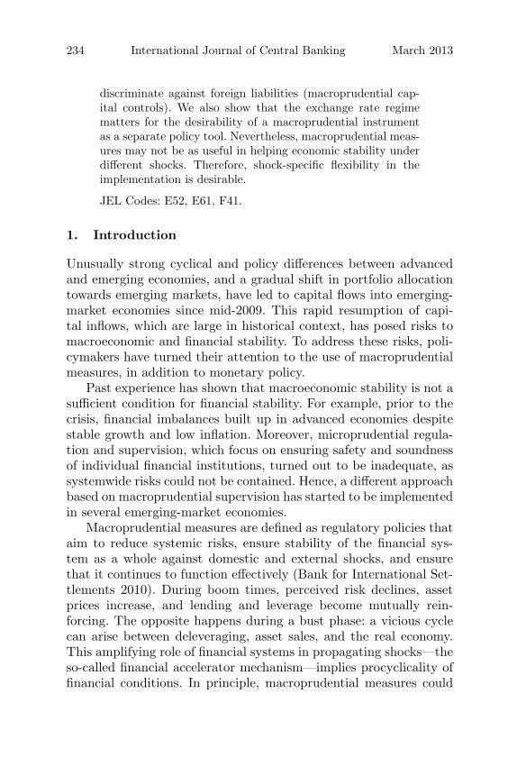
Figure 2. A Positive Financial Shock: BroadMacroprudential Policy and Macroprudential Capital
Controls under Taylor Rule (percent deviationsfrom the steady state)
Notes: The figures show the impact of a 1 percent positive shock to the per-ception of investors regarding the productivity of domestic entrepreneurs. Thevariables are presented as log-deviations from the steady state (except for interestrate), multiplied by 100 to have an interpretation of percentage deviations.
regulation premium only applies to the loans from internationalresources, equation (18), and the regulation premium is defined asa function of the nominal foreign credit growth. Under that sce-nario, the effect of the financial shock on foreign borrowing is less
260 International Journal of Central Banking March 2013
pronounced; the surge in the capital flows is almost two-thirds ofthe baseline case, and the exchange rate appreciates less. Never-theless, the policy measure fails to achieve its very first objectiveof promoting financial stability—it only brings a shift from foreignloans to domestic loans, leaving the aggregate credit growth nearlyunchanged compared with the baseline scenario (figure 1).24
If the shock comes initially from increased optimism of the foreigninvestors only, macroprudential capital controls could help to alle-viate financial instability risk at its source, making broad measuresredundant. In this case, the performance of macroprudential capitalcontrols improves upon a more general macroprudential approach. Inpractice, however, the perceptions of domestic and foreign investorsare unlikely to deviate from each other for a prolonged period,hence we assume away the possibility of a foreign- (or domestic-)investors-specific perception shock.
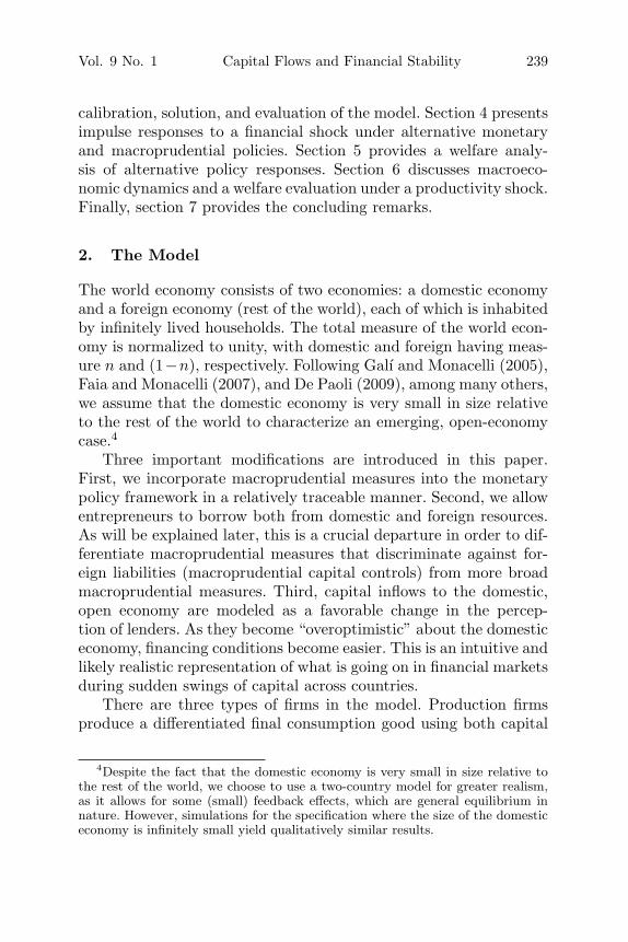
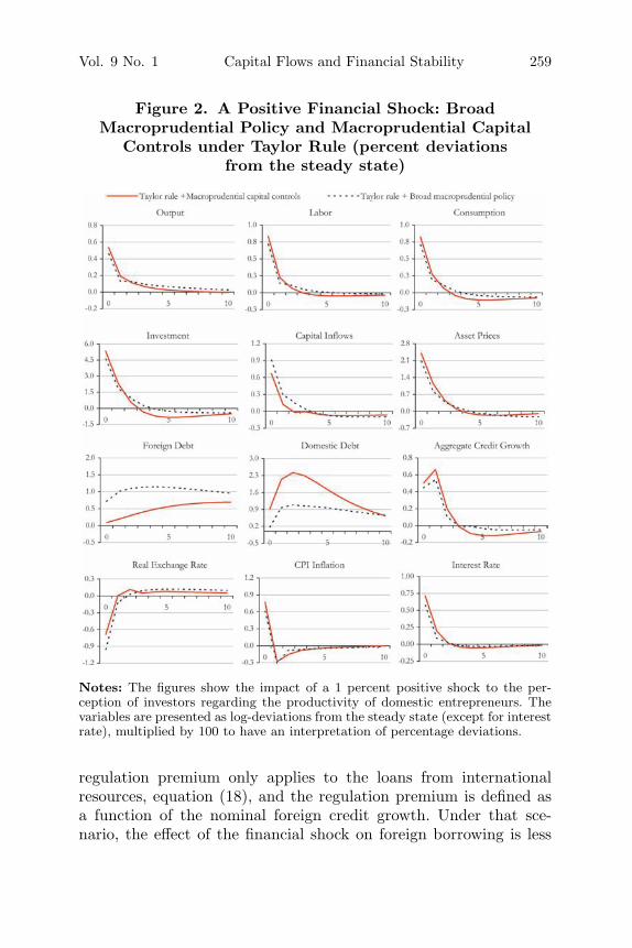
4.3 Does the Exchange Rate Regime Matter for the Role ofMacroprudential Policies?
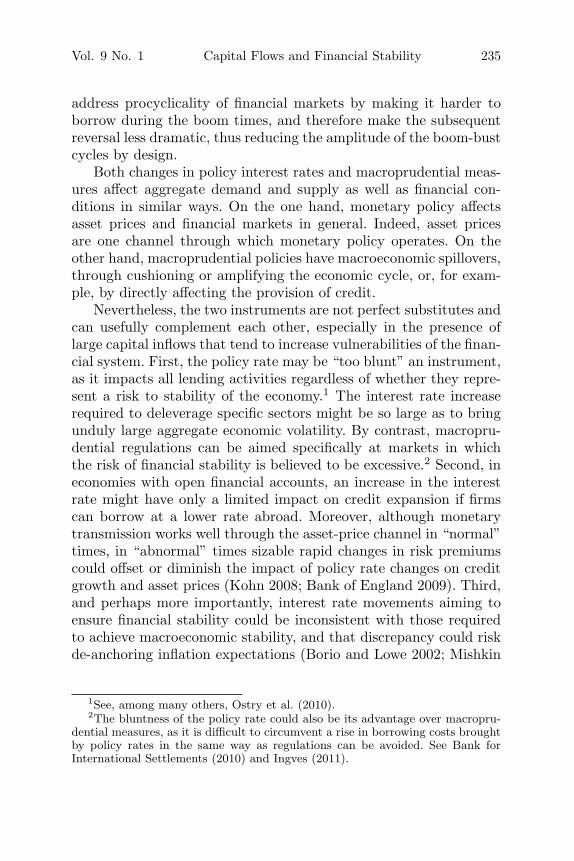
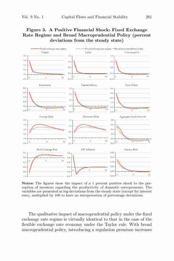
We next analyze the dynamic responses of the macroeconomic vari-ables to the financial shock under a fixed exchange rate regime withand without broad macroprudential policy (figure 3). Under the fixedexchange rate regime, consumption, output, and inflation increaseby about 25 percent more than under the Taylor rule (figure 1)where the nominal currency appreciation helps to limit the over-heating and inflation pressures. The increase in asset prices with thefixed exchange rate regime is also about 20 percent higher than theresponse with the Taylor rule. The responses of foreign and domesticcredit, however, are more muted due to the absence of the positiveimpact of exchange rate appreciation on the net worth of entrepre-neurs, which would make borrowing cheaper by lowering the defaultpremium under the flexible exchange rate regime.
24Macroprudential measures could also be applied to domestic borrowing only.For example, a number of emerging-market countries such as China, Korea, andTurkey have recently increased reserve requirement rates in an effort to tightenmonetary conditions. Nevertheless, similarly to the case of capital controls, sucha measure is likely to bring a shift in the source of borrowing from domestic toforeign markets, causing only a limited change in the aggregate credit growth.
Vol. 9 No. 1 Capital Flows and Financial Stability 261
Figure 3. A Positive Financial Shock: Fixed ExchangeRate Regime and Broad Macroprudential Policy (percent
deviations from the steady state)
Notes: The figures show the impact of a 1 percent positive shock to the per-ception of investors regarding the productivity of domestic entrepreneurs. Thevariables are presented as log-deviations from the steady state (except for interestrate), multiplied by 100 to have an interpretation of percentage deviations.
The qualitative impact of macroprudential policy under the fixedexchange rate regime is virtually identical to that in the case of theflexible exchange rate economy under the Taylor rule. With broadmacroprudential policy, introducing a regulation premium increases
262 International Journal of Central Banking March 2013
the effective lending rate for foreign and domestic entrepreneurs andreduces the impact of the shock on credit growth and investment.Overall, under the fixed exchange rate regime, macroeconomic andfinancial stability implications of the shock are more muted whenbroad macroprudential policy is in place.
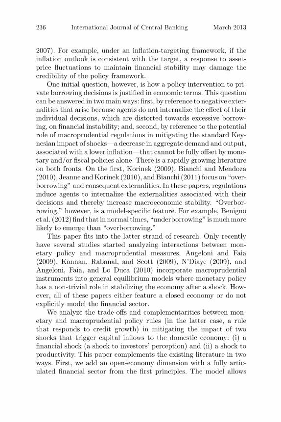
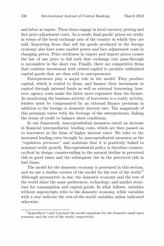
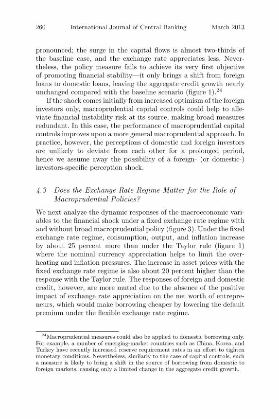
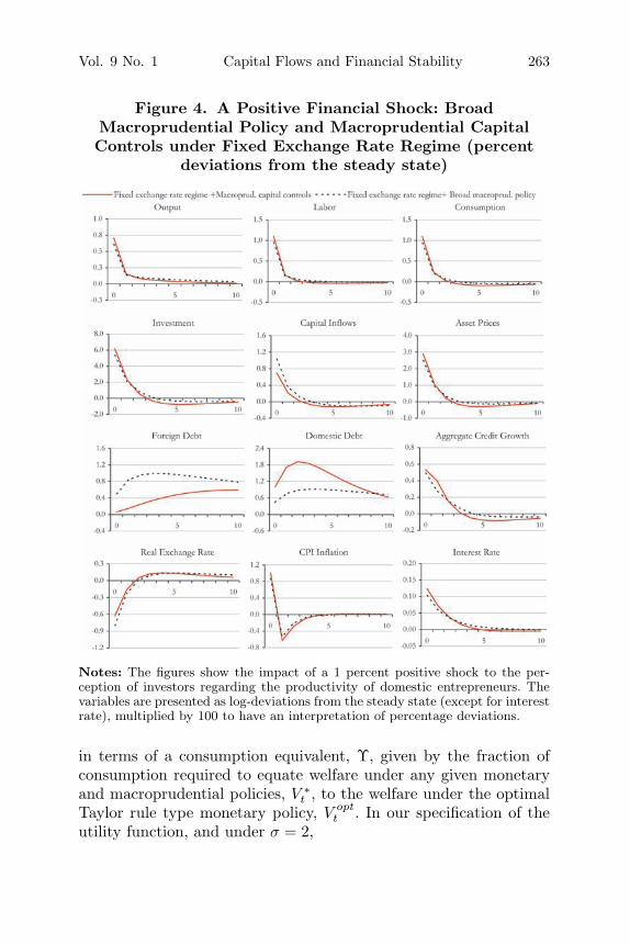
We further investigate the impact of macroprudential capitalcontrols under the fixed exchange rate regime (figure 4). Similar tothe case under the flexible exchange rate regime, the macropruden-tial capital controls are less effective than the broad macroprudentialmeasures in our simulations. Under the fixed exchange rate regime,the responses of capital inflows and real exchange rate are smallerwith macroprudential capital controls, but the responses of assetprices, output, and inflation are almost identical to the case withouta macroprudential tool.
5. Welfare Evaluation of Alternative Policy Options andthe Optimal Policy
To provide a full assessment of optimal policy design, we considerwelfare gains from responding to financial market developments—proxied by nominal credit growth in our experiments—throughmacroprudential policy instruments and compute the optimal degreeof intervention. We take the utility function of consumers as theobjective.
Following Faia and Monacelli (2007) and Gertler and Karadi(2011), we start by expressing the household utility function recur-sively:
Vt = U(Ct, Ht) + βEtVt+1, (22)
where Vt ≡ E0
∞∑t=0
βtU(Ct, Ht) denotes the utility function. We take
a second-order approximation of Vt around the deterministic steadystate. Using the second-order solution of the model, we then cal-culate Vt in each of the separate cases of monetary and macropru-dential policies.25 We do the comparison among alternative policies
25It is rather standard in the literature to calculate the welfare using a second-order approximation to utility function. See Schmitt-Grohe and Uribe (2007) fora lengthy discussion on the topic.
Vol. 9 No. 1 Capital Flows and Financial Stability 263
Figure 4. A Positive Financial Shock: BroadMacroprudential Policy and Macroprudential CapitalControls under Fixed Exchange Rate Regime (percent
deviations from the steady state)
Notes: The figures show the impact of a 1 percent positive shock to the per-ception of investors regarding the productivity of domestic entrepreneurs. Thevariables are presented as log-deviations from the steady state (except for interestrate), multiplied by 100 to have an interpretation of percentage deviations.
in terms of a consumption equivalent, Υ, given by the fraction ofconsumption required to equate welfare under any given monetaryand macroprudential policies, V ∗
t , to the welfare under the optimalTaylor rule type monetary policy, V opt
t . In our specification of theutility function, and under σ = 2,
264 International Journal of Central Banking March 2013
Υ =
((V opt
t − Vt)(1 − β)(C − χ1+ϕH1+ϕ)2
C(1 − (V optt − Vt)(1 − β)(C − χ
1+ϕH1+ϕ))
), (23)
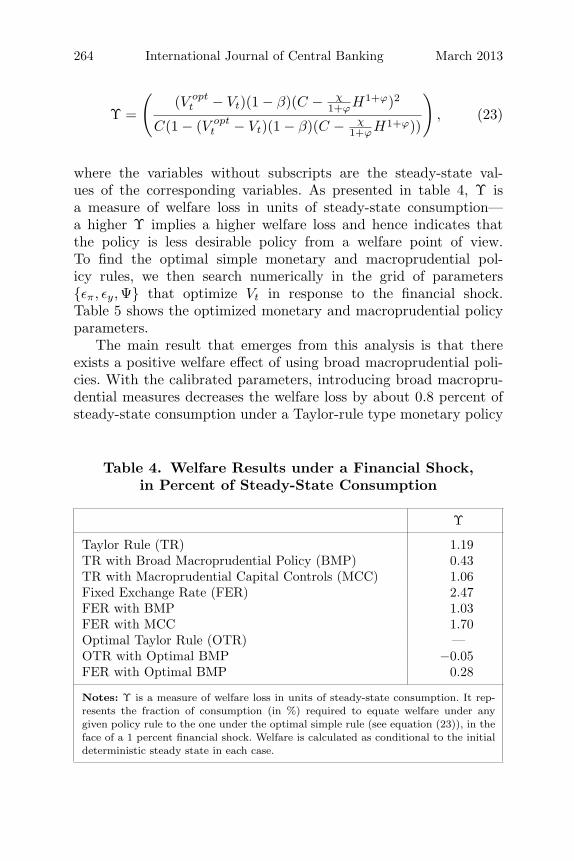
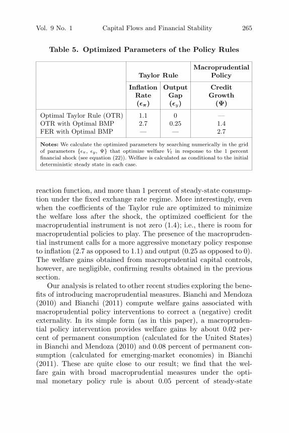
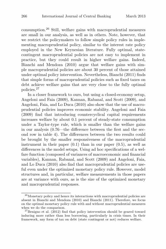
where the variables without subscripts are the steady-state val-ues of the corresponding variables. As presented in table 4, Υ isa measure of welfare loss in units of steady-state consumption—a higher Υ implies a higher welfare loss and hence indicates thatthe policy is less desirable policy from a welfare point of view.To find the optimal simple monetary and macroprudential pol-icy rules, we then search numerically in the grid of parameters{επ, εy, Ψ} that optimize Vt in response to the financial shock.Table 5 shows the optimized monetary and macroprudential policyparameters.
The main result that emerges from this analysis is that thereexists a positive welfare effect of using broad macroprudential poli-cies. With the calibrated parameters, introducing broad macropru-dential measures decreases the welfare loss by about 0.8 percent ofsteady-state consumption under a Taylor-rule type monetary policy
Table 4. Welfare Results under a Financial Shock,in Percent of Steady-State Consumption
Υ
Taylor Rule (TR) 1.19TR with Broad Macroprudential Policy (BMP) 0.43TR with Macroprudential Capital Controls (MCC) 1.06Fixed Exchange Rate (FER) 2.47FER with BMP 1.03FER with MCC 1.70Optimal Taylor Rule (OTR) —OTR with Optimal BMP −0.05FER with Optimal BMP 0.28
Notes: Υ is a measure of welfare loss in units of steady-state consumption. It rep-resents the fraction of consumption (in %) required to equate welfare under anygiven policy rule to the one under the optimal simple rule (see equation (23)), in theface of a 1 percent financial shock. Welfare is calculated as conditional to the initialdeterministic steady state in each case.
Vol. 9 No. 1 Capital Flows and Financial Stability 265
Table 5. Optimized Parameters of the Policy Rules
MacroprudentialTaylor Rule Policy
Inflation Output CreditRate Gap Growth(επ) (εy) (Ψ)
Optimal Taylor Rule (OTR) 1.1 0 —OTR with Optimal BMP 2.7 0.25 1.4FER with Optimal BMP — — 2.7
Notes: We calculate the optimized parameters by searching numerically in the gridof parameters {επ , εy , Ψ} that optimize welfare Vt in response to the 1 percentfinancial shock (see equation (22)). Welfare is calculated as conditional to the initialdeterministic steady state in each case.
reaction function, and more than 1 percent of steady-state consump-tion under the fixed exchange rate regime. More interestingly, evenwhen the coefficients of the Taylor rule are optimized to minimizethe welfare loss after the shock, the optimized coefficient for themacroprudential instrument is not zero (1.4); i.e., there is room formacroprudential policies to play. The presence of the macropruden-tial instrument calls for a more aggressive monetary policy responseto inflation (2.7 as opposed to 1.1) and output (0.25 as opposed to 0).The welfare gains obtained from macroprudential capital controls,however, are negligible, confirming results obtained in the previoussection.
Our analysis is related to other recent studies exploring the bene-fits of introducing macroprudential measures. Bianchi and Mendoza(2010) and Bianchi (2011) compute welfare gains associated withmacroprudential policy interventions to correct a (negative) creditexternality. In its simple form (as in this paper), a macropruden-tial policy intervention provides welfare gains by about 0.02 per-cent of permanent consumption (calculated for the United States)in Bianchi and Mendoza (2010) and 0.08 percent of permanent con-sumption (calculated for emerging-market economies) in Bianchi(2011). These are quite close to our result; we find that the wel-fare gain with broad macroprudential measures under the opti-mal monetary policy rule is about 0.05 percent of steady-state
266 International Journal of Central Banking March 2013
consumption.26 Still, welfare gains with macroprudential measuresare small in our analysis, as well as in others. Note, however, thatwe restrict the policymakers to follow simple policy rules in imple-menting macroprudential policy, similar to the interest rate policyemployed in the New Keynesian literature. Fully optimal, state-contingent macroprudential policies are not easy to implement inpractice, but they could result in higher welfare gains. Indeed,Bianchi and Mendoza (2010) argue that welfare gains with sim-ple macroprudential policies are about 30 percent of those attainedunder optimal policy intervention. Nevertheless, Bianchi (2011) findsthat simple forms of macroprudential policies such as fixed taxes ondebt achieve welfare gains that are very close to the fully optimalpolicies.27
In a closer framework to ours, but using a closed-economy setup,Angeloni and Faia (2009), Kannan, Rabanal, and Scott (2009), andAngeloni, Faia, and Lo Duca (2010) also show that the use of macro-prudential policies improves economic stability. Angeloni and Faia(2009) find that introducing countercyclical capital requirementsincreases welfare by about 0.1 percent of steady-state consumptionunder a Taylor-type rule, which is smaller than the welfare gainsin our analysis (0.76—the difference between the first and the sec-ond row in table 4). The differences between the two results couldbe brought by the smaller responsiveness of the macroprudentialinstrument in their paper (0.1) than in our paper (0.5), as well asdifferences in the model setups. Using ad hoc specifications of a wel-fare function (composed of variances of macroeconomic and financialvariables), Kannan, Rabanal, and Scott (2009) and Angeloni, Faia,and Lo Duca (2010) also find that macroprudential policies are use-ful even under the optimized monetary policy rule. However, modelstructures and, in particular, welfare measurements in those papersare at variance with ours, as is the size of the optimized monetaryand macroprudential responses.
26Monetary policy and hence its interactions with macroprudential policies areabsent in Bianchi and Mendoza (2010) and Bianchi (2011). Therefore, we focuson the optimal monetary policy rule with and without macroprudential measureswhen we do the comparison.
27Benigno et al. (2012) find that policy intervention should be geared towardinducing more rather than less borrowing, particularly in crisis times. In theirframework, any form of tax on debt (state contingent or not) reduces welfare.
Vol. 9 No. 1 Capital Flows and Financial Stability 267
The analysis yields another important result—the exchange rateregime matters for the desirability of using macroprudential poli-cies. The optimized coefficient for the broad macroprudential policyinstrument is higher under the fixed exchange rate regime (2.7) thanunder the Taylor-rule type of monetary policy regime (1.4). Theintuition for why is as follows. Under the Taylor rule, the interestrate rises in response to rising inflation and output. The rise in theinterest rate decreases consumption and investment but also lim-its the increase credit growth. Under a fixed exchange rate regime,the impact of the shock on the economy is more dramatic giventhe absence of an independent interest rate tool, which puts moreof the burden on macroprudential policies to provide macroeconomicand financial stability.28
Focusing exclusively on capital controls, Schmitt-Grohe andUribe (2012) calculate that welfare gains associated with macropru-dential policies are about 2 to 5 percent of steady-state consumption,close to our result of 2.2 percent (the difference between the fourthand the last row in table 4). Similarly, Farhi and Werning (2012)conjecture that intervention measures lean less against the windwhen the exchange rate is flexible than when the exchange rate isfixed.29
6. How Do Macroprudential Measures PerformFollowing a Productivity Shock?
We have analyzed so far the role of macroprudential measures inmacroeconomic policymaking under a financial shock, an exogenouschange in investors’ perception about the entrepreneurs’ produc-tivity. Under that scenario, the responses of monetary policy andmacroprudential measures are aligned (both are contractionary).
28Country experiences seem to support this result. For example, Lim et al.(2011) find that economies with fixed or managed exchange rate regimes tend touse macroprudential tools more frequently.
29Both Schmitt-Grohe and Uribe (2012) and Farhi and Werning (2012) allowonly foreign borrowing in their model. Hence, capital controls in these papersare not selective in nature, and by construction there is no difference betweenbroad macroprudential measures and macroprudential capital controls in effec-tive terms. Therefore, our welfare results with broad macroprudential measuresunder the fixed exchange rate regime are comparable with theirs.
268 International Journal of Central Banking March 2013
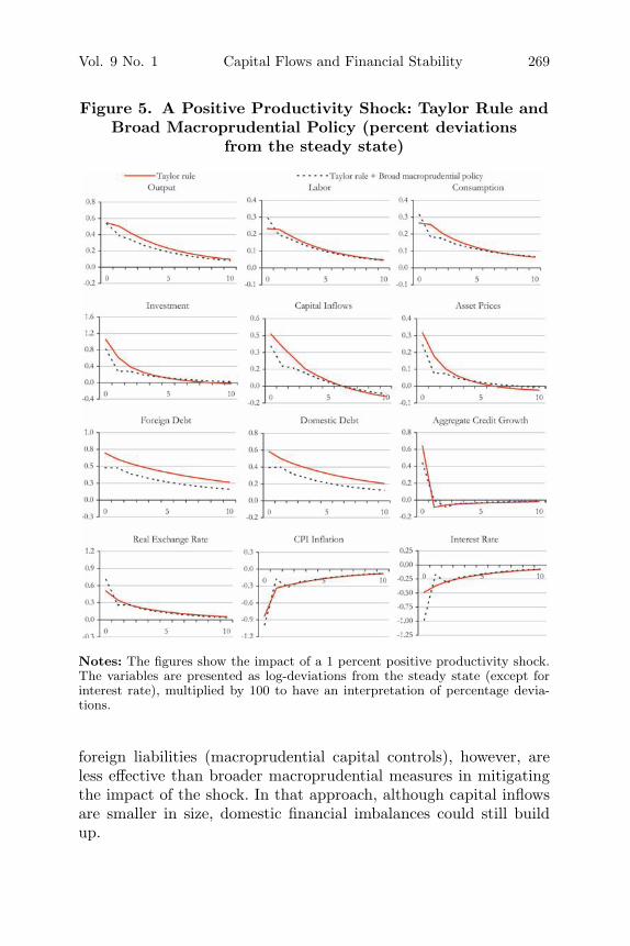
However, there could be other shocks that generate a trade-offbetween macroeconomic and financial stability objectives. For exam-ple, under a productivity shock, entrepreneurs increase their bor-rowings, and investment and asset prices rise as in the previousscenario. On the one hand, inflation declines, and the monetaryauthority responds by decreasing the interest rate under the Taylorrule (figure 5). On the other hand, macroprudential measures callfor a higher lending rate in order to dampen the expanding leveragein the economy.
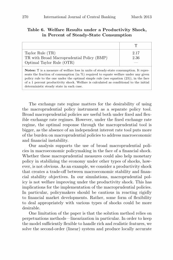
Overall, simulations show that stabilization benefits of introduc-ing macroprudential measures decline under a productivity shock.When broad macroprudential policy is implemented, the outputresponse changes only marginally, while the response of inflationis even higher and the policy rate is lowered by almost two timesmore relative to the case without macroprudential policies. In fact,under a productivity shock, macroprudential measures are not wel-fare improving (table 6). Not surprisingly, the coefficient of themacroprudential instrument that maximizes welfare turns out to bezero.
Kannan, Rabanal, and Scott (2009) and Angeloni, Faia, and LoDuca (2010) also find that the desirability of macroprudential meas-ures is sizably reduced under a productivity shock. Despite the factthat their welfare measurements and model setups are different thanours, both of these papers find that the optimal response througha macroprudential instrument is much smaller under a productivityshock relative to the case under a financial shock.
7. Conclusions
This paper has developed an open-economy DSGE model to inves-tigate whether there is a potential role for macroprudential poli-cies in helping monetary policy stabilize the economy. The sim-ulations suggest that macroprudential tools could be useful attimes in helping to achieve twin objectives of macroeconomic andfinancial stability. In particular, broad macroprudential measuresare shown to improve welfare in the case of a surge in capitalinflows triggered by a financial optimism shock. Even under theoptimal monetary policy rule, broad macroprudential measures arestill beneficial. Macroprudential measures that discriminate against
Vol. 9 No. 1 Capital Flows and Financial Stability 269
Figure 5. A Positive Productivity Shock: Taylor Rule andBroad Macroprudential Policy (percent deviations
from the steady state)
Notes: The figures show the impact of a 1 percent positive productivity shock.The variables are presented as log-deviations from the steady state (except forinterest rate), multiplied by 100 to have an interpretation of percentage devia-tions.
foreign liabilities (macroprudential capital controls), however, areless effective than broader macroprudential measures in mitigatingthe impact of the shock. In that approach, although capital inflowsare smaller in size, domestic financial imbalances could still buildup.
270 International Journal of Central Banking March 2013
Table 6. Welfare Results under a Productivity Shock,in Percent of Steady-State Consumption
Υ
Taylor Rule (TR) 2.17TR with Broad Macroprudential Policy (BMP) 2.36Optimal Taylor Rule (OTR) —
Notes: Υ is a measure of welfare loss in units of steady-state consumption. It repre-sents the fraction of consumption (in %) required to equate welfare under any givenpolicy rule to the one under the optimal simple rule (see equation (23)), in the faceof a 1 percent productivity shock. Welfare is calculated as conditional to the initialdeterministic steady state in each case.
The exchange rate regime matters for the desirability of usingthe macroprudential policy instrument as a separate policy tool.Broad macroprudential policies are useful both under fixed and flex-ible exchange rate regimes. However, under the fixed exchange rateregime, the optimal response through the macroprudential tool isbigger, as the absence of an independent interest rate tool puts moreof the burden on macroprudential policies to address macroeconomicand financial instability.
Our analysis supports the use of broad macroprudential poli-cies in macroeconomic policymaking in the face of a financial shock.Whether these macroprudential measures could also help monetarypolicy in stabilizing the economy under other types of shocks, how-ever, is not obvious. As an example, we consider a productivity shockthat creates a trade-off between macroeconomic stability and finan-cial stability objectives. In our simulations, macroprudential pol-icy is not welfare improving under the productivity shock. This hasimplications for the implementation of the macroprudential policies.In particular, policymakers should be cautious in reacting rigidlyto financial market developments. Rather, some form of flexibilityto deal appropriately with various types of shocks could be moredesirable.
One limitation of the paper is that the solution method relies onperpetuations methods—linearization in particular. In order to keepthe model sufficiently flexible to handle rich and realistic features, wesolve the second-order (linear) system and produce locally accurate

Vol. 9 No. 1 Capital Flows and Financial Stability 271
approximations to the dynamics of the model, without consideringglobal (non-linear) approximations. We acknowledge, however, thatour framework abstracts from non-linearities that seem to play animportant role in financial crises, and interactions between the expost policy interventions in financial markets and the ex ante buildupof risk; and our welfare analysis is limited to the deterministic steadystate as opposed to the stationary distribution.
Although the way macroprudential measures are modeled in thispaper is intuitive, it does not allow us to focus on a particular typeof these measures, such as reserve requirements or capital require-ments. To address this issue, we are extending the model with afully optimized banking sector, which would also make it possible toderive the regulation premium from microfoundations.
Appendix 1. Model Equations: Domestic Economy
Households
Demand functions for home and foreign goods are derived fromthe household’s minimization of expenditure, conditional on totalcomposite demand, and are as follows:
CH,t = (1 − α)(
PH,t
Pt
)−γ
Ct, (24)
CM,t = α
(PM,t
Pt
)−γ
Ct, (25)
and the corresponding price index is given by
Pt = [(1 − α)P 1−γH,t + αP 1−γ
M,t ]1/(1−γ), (26)
where PH,t and PM,t represent the prices for domestic and importedgoods and Pt denotes the consumer price index (CPI).
The representative household chooses the paths for {Ct, Ht,DD
t+1, DHt+1}∞
t=0 in order to maximize its expected lifetime utility inequation (1) subject to the budget constraint in equation (3). Thefirst-order conditions for this optimization problem are given by
272 International Journal of Central Banking March 2013
χHϕt = Wt, (27)(
Ct − χ
1 + ϕH1+ϕ
t
)−σ
= β(1 + it)Et
[(Ct+1 − χ
1 + ϕH1+ϕ
t+1
)−σPt
Pt+1
], (28)
(Ct − χ
1 + ϕH1+ϕ
t
)−σ
= β(1 + i∗t )ΨD,tEt
[(Ct+1 − χ
1 + ϕH1+ϕ
t+1
)−σPt
Pt+1
St+1
St
].
(29)
In the absence of the premium paid on foreign borrowing (ΨD,t),the last two equations would yield the standard uncovered interestrate parity condition.
Production Firms
Assuming that the price of each input is taken as given, the pro-duction firms minimize their costs subject to (4). Omitting the firm-specific indices for notational simplicity, cost-minimizing behaviorimplies the following first-order conditions:
Wt =(1 − η)(1 − Ω)YtMCt
Nt, (30)
WEt = (1 − η)ΩYtMCt, (31)
Rt =ηYtMCt
Kt, (32)
where WEt is the entrepreneurial wage rate, Rt is the rental rate of
capital, and MCt is the (nominal) marginal cost given by MCt =Rη
t W 1−ηt
Atηη(1−η)1−η .
Let YX,t denote the foreign aggregate export demand for domes-tic goods which is determined in the foreign economy (see appen-dix 2). Since the profit-maximization condition is symmetric amongfirms, the optimal price-setting equations can be written in aggregateterms. Using equations (5) and (6) in the text, we derive
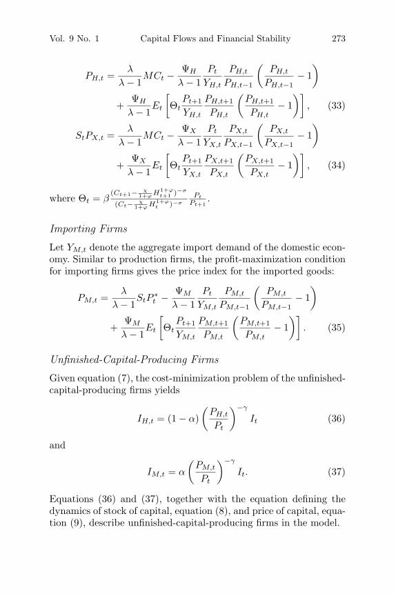
Vol. 9 No. 1 Capital Flows and Financial Stability 273
PH,t =λ
λ − 1MCt − ΨH
λ − 1Pt
YH,t
PH,t
PH,t−1
(PH,t
PH,t−1− 1
)
+ΨH
λ − 1Et
[Θt
Pt+1
YH,t
PH,t+1
PH,t
(PH,t+1
PH,t− 1
)], (33)
StPX,t =λ
λ − 1MCt − ΨX
λ − 1Pt
YX,t
PX,t
PX,t−1
(PX,t
PX,t−1− 1
)
+ΨX
λ − 1Et
[Θt
Pt+1
YX,t
PX,t+1
PX,t
(PX,t+1
PX,t− 1
)], (34)
where Θt = β(Ct+1− χ
1+ϕ H1+ϕt+1 )−σ
(Ct− χ1+ϕ H1+ϕ
t )−σ
Pt
Pt+1.
Importing Firms
Let YM,t denote the aggregate import demand of the domestic econ-omy. Similar to production firms, the profit-maximization conditionfor importing firms gives the price index for the imported goods:
PM,t =λ
λ − 1StP
∗t − ΨM
λ − 1Pt
YM,t
PM,t
PM,t−1
(PM,t
PM,t−1− 1
)
+ΨM
λ − 1Et
[Θt
Pt+1
YM,t
PM,t+1
PM,t
(PM,t+1
PM,t− 1
)]. (35)
Unfinished-Capital-Producing Firms
Given equation (7), the cost-minimization problem of the unfinished-capital-producing firms yields
IH,t = (1 − α)(
PH,t
Pt
)−γ
It (36)
and
IM,t = α
(PM,t
Pt
)−γ
It. (37)
Equations (36) and (37), together with the equation defining thedynamics of stock of capital, equation (8), and price of capital, equa-tion (9), describe unfinished-capital-producing firms in the model.
274 International Journal of Central Banking March 2013
Entrepreneurs
We omit entrepreneur index k for notational simplicity. The con-tract between the lender and the entrepreneur characterizes a defaultthreshold, ωv
t+1, such that if ωvt+1 ≥ ωv
t+1, the lender receives afixed return in the form of a contracted interest on the debt. Ifωv
t+1 < ωvt+1, then the borrower defaults; the lender audits by pay-
ing the monitoring cost and keeps what it finds. Therefore, we candefine the expected return to entrepreneurs v = F, D and lenders,respectively, as follows (ignoring entrepreneur specific):
Et
[RK
t+1QtKvt+1
(∫ ∞
ωvt+1
ωvf(ωv )dωv − ωvt+1
∫ ∞
ωt+1
f(ωv )dωv
)]
= Et[RKt+1QtK
vt+1z
v (ωvt+1)], (38)
Et
[RK
t+1QtKvt+1
(ωv∗
t+1
∫ ∞
ωvt+1
f(ωv∗)dωv∗
+ (1 − μ)∫ ωv
t+1
0ωv∗
t+1f(ωv∗)dωv∗
)]
= Et[RKt+1QtK
vt+1g
v (ωvt+1; �
vt )], (39)
where RKt denotes the ex post realization of return to capital and
is the same regardless of the source of the financing due to arbi-trage. zv (ω) is the borrowers’ share of the total return. We use thedefinition of the lender’s perception of productivity shock ωv∗
t+1 inequation (39), where gv (ωv ; �v ) represents the lender’s share of thetotal return, itself a function of both the idiosyncratic shock and theperception factor.
For domestic and foreign lenders, the opportunity cost of lendingto the entrepreneur is the domestic interest rate (1+ it) and (1+ i∗t ).Thus the loan contract must satisfy the following for the lenders tobe willing to participate in it:
Et
[RK
t+1QtKFt+1
St+1gF (ωF
t+1; �Ft )
]= (1 + i∗t )D
Ft+1, (40)
Et[RKt+1QtK
Dt+1g
D(ωDt+1; �
Dt )] = (1 + it)DD
t+1. (41)
Vol. 9 No. 1 Capital Flows and Financial Stability 275
The contracting problem identifies the capital demand of entre-preneurs, Kv
t+1, and a cut-off value, ωvt+1, such that the entrepre-
neurs will maximize (38) subject to (40) and (41). The first-orderconditions yield (12)–(15) in the text.
Given that the borrower’s and the lender’s share of total returnshould add up to zv (ωv
t )+ gv (ωvt , �v
t ) = 1− νvt (where νv
t is the costof monitoring, a deadweight loss associated with financial frictions)and by using the participation constraints (40) and (41), we canrewrite foreign and domestic borrowing entrepreneurs’ net worth as
PtNWFt = ϑ[RK
t Qt−1KFt (1 − νF
t ) − (1 + i∗t−1)StDFt ] + WFE
t ,(42)
PtNWDt = ϑ[RK
t Qt−1KDt (1 − νD
t ) − (1 + it−1)DDt ] + WDE
t . (43)
The entrepreneurs leaving the scene at time t consume their returnon capital. The consumption of the exiting entrepreneurs, CvE
t , canthen be written as
PtCFEt = (1 − ϑ)[RK
t Qt−1KFt (1 − νF
t ) − (1 + i∗t−1)StDFt ], (44)
PtCDEt = (1 − ϑ)[RK
t Qt−1KDt (1 − νD
t ) − (1 + it−1)DDt ]. (45)
It is assumed that the entrepreneurs consume an identical mixof domestic and foreign goods in their consumption basket withthe households given in equation (2). Therefore the entrepreneurs’demand functions for domestic and imported consumption goods aregiven by
CvEH,t = (1 − α)
(PH,t
Pt
)−γ
CvEt , (46)
CvEM,t = α
(PM,t
Pt
)−γ
CvEt . (47)
To define zv (ω) and gv (ωv ; �v ), we use the relationship between thefunctions erf(.) and erfc(.) and the cumulative distribution functionof a standard normal distribution Θ(.):
erf(x) = 2Θ(x√
2) − 1,
erfc(x) = 2(1 − Θ(x√
2)). (48)
276 International Journal of Central Banking March 2013
Using (48) and two artificial variables zv1t = ln ωv
t +0.5σv2ω
σvω
and
zv2t =
ln(ωv
tt
)+0.5σv2ω
σvω
, we redefine zv (.), gv (.), zv ′(.), and gv ′(.):
zv (ωvt ) = 1 − Θ(zv
1t − σvω) − ωv
t (1 − Θ(zv1t)), (49)
gv (ωvt ; �t) = �t
[ωv
t
�t(1 − Θ(zv
2t)) + (1 − μ)Θ(zv2t − σv
ω)]
, (50)
zv ′(ωvt ) = −(1 − Θ(zv
1t)), (51)
gv ′(ωvt ; �t) = �t
[1 − Θ(zv
2t) − μ√2πσv
ω
exp(
−zv22t
2
)]. (52)
Equations (40)–(52), together with (12)–(17), form the entrepre-neurs block of the model.
Financial Intermediaries and Macroprudential Policy
Model equations for financial intermediaries and macroprudentialpolicies are given in (18)–(20).
Monetary Policy
In the baseline case, we assume that monetary policy reaction func-tion follows a Taylor-type rule with interest rate smoothing as givenin (21).
General Equilibrium and Balance-of-Payments Dynamics
Market clearing in the final good sector requires that total domes-tic output be equal to domestic consumption, domestic investment,and exports to the rest of the world. Frictions such as adjustmentand monitoring costs are included in the output, given that theyare expressed in terms of the final composite good. Thus the overallresource constraint faced by the domestic economy can be written as
Yt = YH,t + YX,t, (53)
Vol. 9 No. 1 Capital Flows and Financial Stability 277
where
YH,t = CH,t + CEH,t + IH,t
+ (1 − α)(
PH,t
Pt
)−γ⎡⎣ ∑
i=H,X
Ψi
2
(Pi,t
Pi,t−1− 1
)2
+ΨM
2
(PM,t
PM,t−1− 1
)2
+∑
j=F,D
νjt
RKt
PtQt−1K
jt
⎤⎦ . (54)
The import demand of the domestic economy (which is the exportof the foreign economy) Y ∗
X,t, can be expressed as follows:
Y ∗X,t = CM,t + CE
M,t + IM,t + α
(PM,t
Pt
)−γ⎡⎣ ∑
i=H,X
Ψi
2
(Pi,t
Pi,t−1− 1
)2
+ΨM
2
(PM,t
PM,t−1− 1
)2
+∑
j=F,D
νjt
RKt
PtQt−1K
jt
⎤⎦ , (55)
where CM,t and CEM,t are demand for imports by households and
entrepreneurs, respectively, and IM,t is the domestic economy’simport demand for investment goods.
Substituting (48) and the profits of both the final-good-producing and the importing firms into the budget constraints ofthe households and the entrepreneurs yields the following balance-of-payments condition after aggregation:
StPX,tYX,t − StP∗t Y ∗
X,t = St(1 + i∗t−1)(DHt ΨD,t−1 + DF
t )
− St(DHt+1 + DF
t+1), (56)
where the first and second terms on the left are exports and imports,respectively. On the right is simply the change in the net foreign assetposition, aggregated over households and entrepreneurs.
278 International Journal of Central Banking March 2013
Appendix 2. Model Equations: The Rest of the World
Apart from being asymmetric in size, the domestic economy and therest of the world share the same preferences, technology, and mar-ket structure for consumption and capital goods. Therefore, we onlypresent equations here for the rest-of-the-world part of the model,and give only brief explanation when necessary.
Households
C∗H,t = (1 − α∗)
(P ∗
H,t
P ∗t
)−γ∗
C∗t , (57)
C∗M,t = α∗
(P ∗
M,t
P ∗t
)−γ∗
C∗t , (58)
P ∗t =
[(1 − α∗)P ∗1−γ∗
H,t + α∗P ∗1−γ∗
M,t
]1/(1−γ∗), (59)
χH∗ϕt = W ∗
t , (60)(C∗
t − χ
1 + ϕH∗1+ϕ
t
)−σ
= β(1 + i∗t )Et
[(C∗
t+1−χ
1 + ϕH∗1+ϕ
t+1
)−σP ∗
t
P ∗t+1
]. (61)
Production Firms
W ∗t =
(1 − η)(1 − Ω)Y ∗t MC∗
t
N∗t
, (62)
W ∗Et = (1 − η)ΩY ∗
t MC∗t , (63)
R∗t =
ηY ∗t MC∗
t
K∗t
, (64)
P ∗H,t =
λ
λ − 1MC∗
t − ΨH
λ − 1P ∗
t
Y ∗H,t
P ∗H,t
P ∗H,t−1
(P ∗
H,t
P ∗H,t−1
− 1
)
+ΨH
λ − 1Et
[Θ∗
t
P ∗t+1
Y ∗H,t
P ∗H,t+1
P ∗H,t
(P ∗
H,t+1
P ∗H,t
− 1
)], (65)
Vol. 9 No. 1 Capital Flows and Financial Stability 279
S∗t P ∗
X,t =λ
λ − 1MC∗
t − ΨX
λ − 1P ∗
t
Y ∗X,t
P ∗X,t
P ∗X,t−1
(P ∗
X,t
P ∗X,t−1
− 1
)
+ΨX
λ − 1Et
[Θ∗
t
P ∗t+1
Y ∗X,t
P ∗X,t+1
P ∗X,t
(P ∗
X,t+1
P ∗X,t
− 1
)], (66)
where Θ∗t = β
(C∗t+1− χ
1+ϕ H∗1+ϕt+1 )−σ
(C∗t − χ
1+ϕ H∗1+ϕt )−σ
P ∗t
P ∗t+1
.
Importing Firms
PM,t =λ
λ − 1S∗
t P ∗t − ΨM
λ − 1Pt
YM,t
PM,t
PM,t−1
(PM,t
PM,t−1− 1
)(67)
+ΨM
λ − 1Et
[Θt
Pt+1
YM,t
PM,t+1
PM,t
(PM,t+1
PM,t− 1
)].
Unfinished-Capital-Producing Firms
I∗H,t = (1 − α∗)
(P ∗
H,t
P ∗t
)−γ
I∗t , (68)
I∗M,t = α∗
(P ∗
M,t
P ∗t
)−γ
I∗t , (69)
K∗t+1 =
[I∗t
K∗t
− ΨI
2
(I∗t
K∗t
− δ
)2]
K∗t + (1 − δ)K∗
t , (70)
Q∗t
P ∗t
=[1 − ΨI
(I∗t
K∗t
− δ
)]−1
. (71)
Entrepreneurs
Entrepreneurs in the rest of the world only borrow domestically intheir own currency.
Et
[RK∗
t+1Q∗t K
∗t+1
(∫ ∞
ω∗t+1
ω∗f(ω∗)dω∗ − ω∗t+1
∫ ∞
ω∗t+1
f(ω∗)dω∗
)]
= Et
[RK∗
t+1Q∗t K
∗t+1z
∗ (ω∗
t+1)]
, (72)
280 International Journal of Central Banking March 2013
Et
[RK∗
t+1Q∗t K
∗t+1
(ω∗
t+1
∫ ∞
ω∗t+1
f(ω∗)dω∗
+ (1 − μ)∫ ω∗
t+1
0ω∗
t+1f(ω∗)dω∗
)]
= Et[RK∗t+1QtK
∗t+1g
∗(ω∗t+1; �
∗t )], (73)
Et[RK∗t+1Q
∗t K
∗t+1g
∗(ω∗t+1; �
∗t )] = (1 + i∗t )D
∗t+1, (74)
P ∗t NW ∗
t = ϑ[RK∗t Q∗
t−1K∗t (1 − ν∗
t ) − (1 + i∗t−1)D∗t ] + WE∗
t , (75)
P ∗t CE∗
t = (1 − ϑ)[RK∗t Q∗
t−1K∗t (1 − ν∗
t ) − (1 + i∗t−1)D∗t ], (76)
CE∗H,t = (1 − α∗)
(P ∗
H,t
P ∗t
)−γ
CE∗t , (77)
CE∗M,t = α∗
(P ∗
M,t
P ∗t
)−γ
CE∗t , (78)
Et[RK∗t+1] = Et[(1 + i∗t )(1 + Φ∗
t+1)], (79)
1 + Φ∗t+1 =
[z∗′(ω∗
t+1)g∗(ω∗
t+1; �∗t )z∗′(ω∗
t+1) − z∗(ω∗t+1)g∗′(ω∗
t+1; �∗t )
], (80)
z∗(ω∗t ) = 1 − Θ(z∗
1t − σ∗ω) − ω∗
t (1 − Θ(z∗1t)), (81)
g∗(ω∗t ; �
∗t ) = �∗
t
[ω∗
t
�∗t
(1 − Θ(z∗2t)) + (1 − μ)Θ(z∗
2t − σ∗ω)
], (82)
z∗′(ω∗t ) = −(1 − Θ(z∗
1t)), (83)
g∗′(ω∗t ; �
∗t ) = �∗
t
[1 − Θ(z∗
2t) − μ√2πσ∗
ω
exp(
−z∗22t
2
), (84)
Et[RK∗t+1] = Et
[R∗
t+1
Q∗t
+Q∗
t+1
Q∗t
{(1 − δ) + ΨI
(I∗t+1
K∗t+1
− δ
)I∗t+1
K∗t+1
− ΨI
2
(I∗t+1
K∗t+1
− δ
)2}]
. (85)
Vol. 9 No. 1 Capital Flows and Financial Stability 281
Financial Intermediaries and Macroprudential Policy
We assume that there is no macroprudential policy in the rest-of-the-world block.
Monetary Policy
1 + i∗t = [(1 + i∗)(π∗t )ε∗
π(Y ∗t /Y ∗)ε∗
Y ]∗[1 + i∗t−1]
1−∗. (86)
General Equilibrium and Balance-of-Payments Dynamics
S∗t = 1/St, (87)
Y ∗t = Y ∗
H,t + Y ∗X,t, (88)
Y ∗H,t = C∗
H,t + CE∗H,t + I∗
H,t
+ (1 − α∗)(
P ∗H,t
P ∗t
)−γ⎡⎣ ∑
i=H,X
Ψi
2
(P ∗
i,t
P ∗i,t−1
− 1
)2
+ΨM
2
(P ∗
M,t
P ∗M,t−1
− 1
)2
+ ν∗t
RK∗t
P ∗t
Q∗t−1K
∗t
⎤⎦ , (89)
YX,t = C∗M,t + CE∗
M,t + I∗M,t + α∗
(P ∗
M,t
P ∗t
)−γ⎡⎣ ∑
i=H,X
Ψi
2
(P ∗
i,t
P ∗i,t−1
− 1
)2
+ΨM
2
(P ∗
M,t
P ∗M,t−1
− 1
)2
+ ν∗t
RK∗t
P ∗t
Q∗t−1K
∗t
⎤⎦ . (90)
References
Angeloni, I., and E. Faia. 2009. “A Tale of Two Policies: Pruden-tial Regulation and Monetary Policy with Fragile Banks.” KielWorking Paper No. 1569.
Angeloni, I., E. Faia, and M. Lo Duca. 2010. “Monetary Policy andRisk Taking.” Bruegel Working Paper.
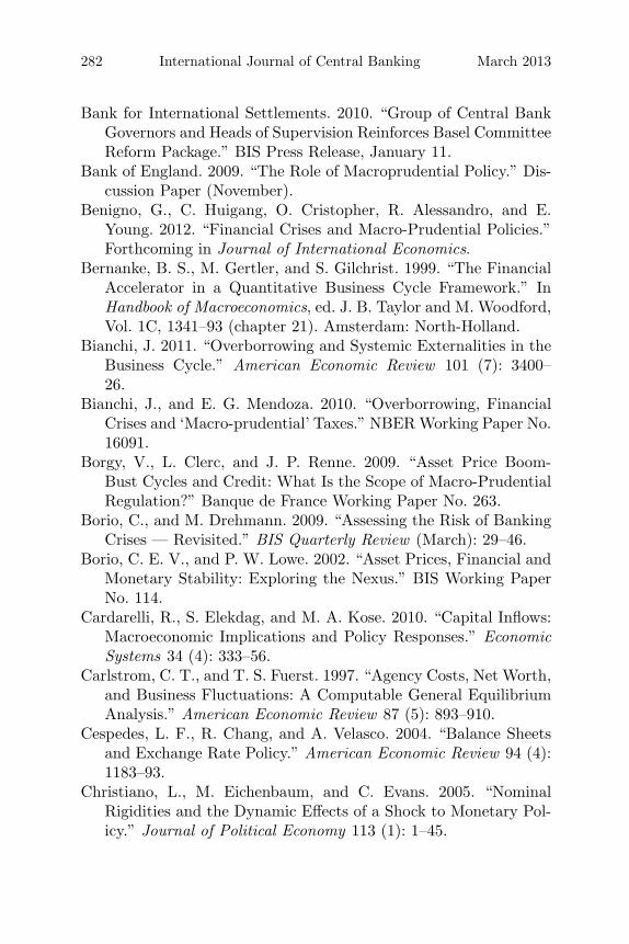
282 International Journal of Central Banking March 2013
Bank for International Settlements. 2010. “Group of Central BankGovernors and Heads of Supervision Reinforces Basel CommitteeReform Package.” BIS Press Release, January 11.
Bank of England. 2009. “The Role of Macroprudential Policy.” Dis-cussion Paper (November).
Benigno, G., C. Huigang, O. Cristopher, R. Alessandro, and E.Young. 2012. “Financial Crises and Macro-Prudential Policies.”Forthcoming in Journal of International Economics.
Bernanke, B. S., M. Gertler, and S. Gilchrist. 1999. “The FinancialAccelerator in a Quantitative Business Cycle Framework.” InHandbook of Macroeconomics, ed. J. B. Taylor and M. Woodford,Vol. 1C, 1341–93 (chapter 21). Amsterdam: North-Holland.
Bianchi, J. 2011. “Overborrowing and Systemic Externalities in theBusiness Cycle.” American Economic Review 101 (7): 3400–26.
Bianchi, J., and E. G. Mendoza. 2010. “Overborrowing, FinancialCrises and ‘Macro-prudential’ Taxes.” NBER Working Paper No.16091.
Borgy, V., L. Clerc, and J. P. Renne. 2009. “Asset Price Boom-Bust Cycles and Credit: What Is the Scope of Macro-PrudentialRegulation?” Banque de France Working Paper No. 263.
Borio, C., and M. Drehmann. 2009. “Assessing the Risk of BankingCrises — Revisited.” BIS Quarterly Review (March): 29–46.
Borio, C. E. V., and P. W. Lowe. 2002. “Asset Prices, Financial andMonetary Stability: Exploring the Nexus.” BIS Working PaperNo. 114.
Cardarelli, R., S. Elekdag, and M. A. Kose. 2010. “Capital Inflows:Macroeconomic Implications and Policy Responses.” EconomicSystems 34 (4): 333–56.
Carlstrom, C. T., and T. S. Fuerst. 1997. “Agency Costs, Net Worth,and Business Fluctuations: A Computable General EquilibriumAnalysis.” American Economic Review 87 (5): 893–910.
Cespedes, L. F., R. Chang, and A. Velasco. 2004. “Balance Sheetsand Exchange Rate Policy.” American Economic Review 94 (4):1183–93.
Christiano, L., M. Eichenbaum, and C. Evans. 2005. “NominalRigidities and the Dynamic Effects of a Shock to Monetary Pol-icy.” Journal of Political Economy 113 (1): 1–45.
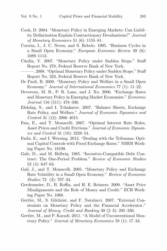
Vol. 9 No. 1 Capital Flows and Financial Stability 283
Cook, D. 2004. “Monetary Policy in Emerging Markets: Can Liabil-ity Dollarization Explain Contractionary Devaluations?” Journalof Monetary Economics 51 (6): 1155–81.
Correia, I., J. C. Neves, and S. Rebelo. 1995. “Business Cycles ina Small Open Economy.” European Economic Review 39 (6):1089–1113.
Curdia, V. 2007. “Monetary Policy under Sudden Stops.” StaffReport No. 278, Federal Reserve Bank of New York.
———. 2008. “Optimal Monetary Policy under Sudden Stops.” StaffReport No. 323, Federal Reserve Bank of New York.
De Paoli, B. 2009. “Monetary Policy and Welfare in a Small OpenEconomy.” Journal of International Economics 77 (1): 11–22.
Devereux, M. B., P. R. Lane, and J. Xu. 2006. “Exchange Ratesand Monetary Policy in Emerging Market Economies.” EconomicJournal 116 (511): 478–506.
Elekdag, S., and I. Tchakarov. 2007. “Balance Sheets, ExchangeRate Policy, and Welfare.” Journal of Economic Dynamics andControl 31 (12): 3986–4015.
Faia, E., and T. Monacelli. 2007. “Optimal Interest Rate Rules,Asset Prices and Credit Frictions.” Journal of Economic Dynam-ics and Control 31 (10): 3228–54.
Farhi, E., and I. Werning. 2012. “Dealing with the Trilemma: Opti-mal Capital Controls with Fixed Exchange Rates.” NBER Work-ing Paper No. 18199.
Gale, D., and M. Hellwig. 1985. “Incentive-Compatible Debt Con-tract: The One-Period Problem.” Review of Economic Studies52 (4): 647–63.
Galı, J., and T. Monacelli. 2005. “Monetary Policy and ExchangeRate Volatility in a Small Open Economy.” Review of EconomicStudies 72 (3): 707–34.
Gerdesmeier, D., B. Roffia, and H. E. Reimers. 2009. “Asset PriceMisalignments and the Role of Money and Credit.” ECB Work-ing Paper No. 1068.
Gertler, M., S. Gilchrist, and F. Natalucci. 2007. “External Con-straints on Monetary Policy and the Financial Accelerator.”Journal of Money, Credit and Banking 39 (2–3): 295–330.
Gertler, M., and P. Karadi. 2011. “A Model of Unconventional Mon-etary Policy.” Journal of Monetary Economics 58 (1): 17–34.
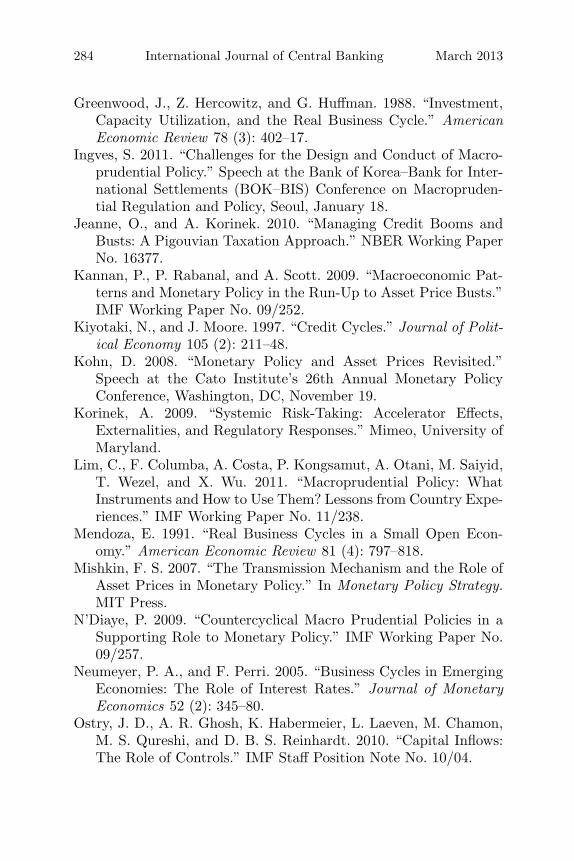
284 International Journal of Central Banking March 2013
Greenwood, J., Z. Hercowitz, and G. Huffman. 1988. “Investment,Capacity Utilization, and the Real Business Cycle.” AmericanEconomic Review 78 (3): 402–17.
Ingves, S. 2011. “Challenges for the Design and Conduct of Macro-prudential Policy.” Speech at the Bank of Korea–Bank for Inter-national Settlements (BOK–BIS) Conference on Macropruden-tial Regulation and Policy, Seoul, January 18.
Jeanne, O., and A. Korinek. 2010. “Managing Credit Booms andBusts: A Pigouvian Taxation Approach.” NBER Working PaperNo. 16377.
Kannan, P., P. Rabanal, and A. Scott. 2009. “Macroeconomic Pat-terns and Monetary Policy in the Run-Up to Asset Price Busts.”IMF Working Paper No. 09/252.
Kiyotaki, N., and J. Moore. 1997. “Credit Cycles.” Journal of Polit-ical Economy 105 (2): 211–48.
Kohn, D. 2008. “Monetary Policy and Asset Prices Revisited.”Speech at the Cato Institute’s 26th Annual Monetary PolicyConference, Washington, DC, November 19.
Korinek, A. 2009. “Systemic Risk-Taking: Accelerator Effects,Externalities, and Regulatory Responses.” Mimeo, University ofMaryland.
Lim, C., F. Columba, A. Costa, P. Kongsamut, A. Otani, M. Saiyid,T. Wezel, and X. Wu. 2011. “Macroprudential Policy: WhatInstruments and How to Use Them? Lessons from Country Expe-riences.” IMF Working Paper No. 11/238.
Mendoza, E. 1991. “Real Business Cycles in a Small Open Econ-omy.” American Economic Review 81 (4): 797–818.
Mishkin, F. S. 2007. “The Transmission Mechanism and the Role ofAsset Prices in Monetary Policy.” In Monetary Policy Strategy.MIT Press.
N’Diaye, P. 2009. “Countercyclical Macro Prudential Policies in aSupporting Role to Monetary Policy.” IMF Working Paper No.09/257.
Neumeyer, P. A., and F. Perri. 2005. “Business Cycles in EmergingEconomies: The Role of Interest Rates.” Journal of MonetaryEconomics 52 (2): 345–80.
Ostry, J. D., A. R. Ghosh, K. Habermeier, L. Laeven, M. Chamon,M. S. Qureshi, and D. B. S. Reinhardt. 2010. “Capital Inflows:The Role of Controls.” IMF Staff Position Note No. 10/04.

Vol. 9 No. 1 Capital Flows and Financial Stability 285
Ozkan, G., and D. F. Unsal. 2010. “External Finance, Sudden Stops,and Financial Crisis: What Is Different this Time?” IMF WorkingPaper No. 10/158.
Rotemberg, J. 1982. “Sticky Prices in the United States.” Journalof Political Economy 90 (6): 1187–1211.
Schmitt-Grohe, S., and M. Uribe. 2003. “Closing Small Open Econ-omy Models.” Journal of International Economics 61 (1): 163–85.
———. 2007. “Optimal Simple and Implementable Monetary andFiscal Rules.” Journal of Monetary Economics 54 (6): 1702–25.
———. 2012. “Prudential Policy for Peggers.” NBER WorkingPaper No. 18031.
Sims, C. 2005. “Second-Order Accurate Solution of Discrete TimeDynamic Equilibrium Models.” Mimeo, Princeton University.