BRITISH STANDARD BS ISO 11843-2:2000Incorporating corrigendum October 2007

Capability of detection —Part 2: Methodology in the linear calibration case

ICS 03.120.30; 17.020

�������������� ���������������������������������������������������

BS ISO 11843-2:2000

This British Standard was published under the authority of the Standards Committee and comes into effect on 15 June 2000

© BSI 2008

ISBN 978 0 580 60989 3

National foreword

This British Standard is the UK implementation of ISO 11843-2:2000, incorporating corrigendum October 2007, which should be read in conjunction with BS ISO 11843-1:2000. The start and finish of text introduced or altered by corrigendum is indicated in the text by tags. Text altered by ISO corrigendum October 2007 is indicated in the text by ˆ‰.The UK participation in its preparation was entrusted to Technical Committee SS/6, Precision of test methods.A list of organizations represented on this committee can be obtained on request to its secretary.This publication does not purport to include all the necessary provisions of a contract. Users are responsible for its correct application.Compliance with a British Standard cannot confer immunity from legal obligations.

Amendments/corrigenda issued since publication

Date Comments

31 March 2008 Implementation of ISO corrigendum October 2007

Reference numberISO 11843-2:2000(E)

INTERNATIONALSTANDARD

ISO11843-2

First edition2000-05-01

Capability of detection —

Part 2:Methodology in the linear calibration case

Capacité de détection —

Partie 2: Méthodologie de l'étalonnage linéaire

BS ISO 11843-2:2000

ii

iii

Contents

Foreword.....................................................................................................................................................................iv

Introduction .................................................................................................................................................................v

1 Scope ..............................................................................................................................................................1

2 Normative references ....................................................................................................................................1

3 Terms and definitions ...................................................................................................................................2

4 Experimental design......................................................................................................................................24.1 General............................................................................................................................................................24.2 Choice of reference states............................................................................................................................24.3 Choice of the number of reference states, I, and the (numbers of) replications of procedure, J,

K and L ............................................................................................................................................................3

5 The critical values yc and xc and the minimum detectable value xd of a measurement series .............35.1 Basic assumptions ........................................................................................................................................35.2 Case 1 — Constant standard deviation.......................................................................................................45.3 Case 2 — Standard deviation linearly dependent on the net state variable............................................6

6 Minimum detectable value of the measurement method ..........................................................................9

7 Reporting and use of results ......................................................................................................................107.1 Critical values...............................................................................................................................................107.2 Minimum detectable values ........................................................................................................................10

Annex A (normative) Symbols and abbreviations .................................................................................................11

Annex B (informative) Derivation of formulae........................................................................................................14

Annex C (informative) Examples .............................................................................................................................20

Bibliography ..............................................................................................................................................................24

BS ISO 11843-2:2000

iv

Foreword

ISO (the International Organization for Standardization) is a worldwide federation of national standards bodies (ISOmember bodies). The work of preparing International Standards is normally carried out through ISO technicalcommittees. Each member body interested in a subject for which a technical committee has been established hasthe right to be represented on that committee. International organizations, governmental and non-governmental, inliaison with ISO, also take part in the work. ISO collaborates closely with the International ElectrotechnicalCommission (IEC) on all matters of electrotechnical standardization.

International Standards are drafted in accordance with the rules given in the ISO/IEC Directives, Part 3.

Draft International Standards adopted by the technical committees are circulated to the member bodies for voting.Publication as an International Standard requires approval by at least 75 % of the member bodies casting a vote.

Attention is drawn to the possibility that some of the elements of this part of ISO 11843 may be the subject ofpatent rights. ISO shall not be held responsible for identifying any or all such patent rights.

International Standard ISO 11843-2 was prepared by Technical Committee ISO/TC 69, Applications of statisticalmethods, Subcommittee SC 6, Measurement methods and results.

ISO 11843 consists of the following parts, under the general title Capability of detection:

� Part 1: Terms and definitions

� Part 2: Methodology in the linear calibration case

Annex A forms a normative part of this part of ISO 11843. Annexes B and C are for information only.

— data are used

— Part 4: Methodology for comparing the minimum detectable value with a given value

— Part 5: Methodology in the linear and non-linear calibration cases

Part 3: Methodology for determination of the critical value for the response variable when no calibration

BS ISO 11843-2:2000

v

Introduction

An ideal requirement for the capability of detection with respect to a selected state variable would be that the actualstate of every observed system can be classified with certainty as either equal to or different from its basic state.However, due to systematic and random distortions, this ideal requirement cannot be satisfied because:

� in reality all reference states, including the basic state, are never known in terms of the state variable. Hence,all states can only be correctly characterized in terms of differences from basic state, i.e. in terms of the netstate variable.

In practice, reference states are very often assumed to be known with respect to the state variable. In otherwords, the value of the state variable for the basic state is set to zero; for instance in analytical chemistry, theunknown concentration or the amount of analyte in the blank material usually is assumed to be zero andvalues of the net concentration or amount are reported in terms of supposed concentrations or amounts. Inchemical trace analysis especially, it is only possible to estimate concentration or amount differences withrespect to available blank material. In order to prevent erroneous decisions, it is generally recommended toreport differences from the basic state only, i.e. data in terms of the net state variable;

NOTE In the ISO Guide 30 and in ISO 11095 no distinction is made between the state variable and the net statevariable. As a consequence, in these two documents reference states are, without justification, assumed to be known withrespect to the state variable.

� the calibration and the processes of sampling and preparation add random variation to the measurementresults.

In this part of ISO 11843, the following two requirements were chosen:

� the probability is ��of detecting (erroneously) that a system is not in the basic state when it is in the basicstate;

� the probability is ���of (erroneously) not detecting that a system, for which the value of the net state variable isequal to the minimum detectable value (xd), is not in the basic state.

BS ISO 11843-2:2000

blank

1

Capability of detection —

Part 2:Methodology in the linear calibration case

1 Scope

This part of ISO 11843 specifies basic methods to:

� design experiments for the estimation of the critical value of the net state variable, the critical value of theresponse variable and the minimum detectable value of the net state variable,

� estimate these characteristics from experimental data for the cases in which the calibration function is linearand the standard deviation is either constant or linearly related to the net state variable.

The methods described in this part of ISO 11843 are applicable to various situations such as checking theexistence of a certain substance in a material, the emission of energy from samples or plants, or the geometricchange in static systems under distortion.

Critical values can be derived from an actual measurement series so as to assess the unknown states of systemsincluded in the series, whereas the minimum detectable value of the net state variable as a characteristic of themeasurement method serves for the selection of appropriate measurement processes. In order to characterize ameasurement process, a laboratory or the measurement method, the minimum detectable value can be stated ifappropriate data are available for each relevant level, i.e. a measurement series, a measurement process, alaboratory or a measurement method. The minimum detectable values may be different for a measurement series,a measurement process, a laboratory or the measurement method.

ISO 11843 is applicable to quantities measured on scales that are fundamentally continuous. It is applicable tomeasurement processes and types of measurement equipment where the functional relationship between theexpected value of the response variable and the value of the state variable is described by a calibration function. Ifthe response variable or the state variable is a vectorial quantity the methods of ISO 11843 are applicableseparately to the components of the vectors or functions of the components.

2 Normative references

The following normative documents contain provisions which, through reference in this text, constitute provisions ofthis part of ISO 11843. For dated references, subsequent amendments to, or revisions of, any of these publicationsdo not apply. However, parties to agreements based on this part of ISO 11843 are encouraged to investigate thepossibility of applying the most recent editions of the normative documents indicated below. For undatedreferences, the latest edition of the normative document referred to applies. Members of ISO and IEC maintainregisters of currently valid International Standards.

ISO 3534-3:1999, Statistics — Vocabulary and symbols — Part 3: Design of experiments.

ISO 3534-1, Statistics — Vocabulary and symbols — Part 1: General statistical terms and terms used in probability

ISO 3534-2, Statistics — Vocabulary and symbols — Part 2: Applied statistics

ˆ

‰

BS ISO 11843-2:2000

2

ISO 11095:1996, Linear calibration using reference materials.

ISO 11843-1:1997, Capability of detection — Part 1: Terms and definitions.

ISO Guide 30:1992, Terms and definitions used in connection with reference materials.

3 Terms and definitions

For the purposes of this part of ISO 11843, the terms and definitions of ISO 3534 (all parts), ISO Guide 30,ISO 11095 and ISO 11843-1 apply.

4 Experimental design

4.1 General

The procedure for determining values of an unknown actual state includes sampling, preparation and themeasurement itself. As every step of this procedure may produce distortion, it is essential to apply the sameprocedure for characterizing, for use in the preparation and determination of the values of the unknown actualstate, for all reference states and for the basic state used for calibration.

For the purpose of determining differences between the values characterizing one or more unknown actual statesand the basic state, it is necessary to choose an experimental design suited for comparison. The experimental unitsof such an experiment are obtained from the actual states to be measured and all reference states used forcalibration. An ideal design would keep constant all factors known to influence the outcome and control of unknownfactors by providing a randomized order to prepare and perform the measurements.

In reality it may be difficult to proceed in such a way, as the preparations and determination of the values of thestates involved are performed consecutively over a period of time. However, in order to detect major biaseschanging with time, it is strongly recommended to perform one half of the calibration before and one half after themeasurement of the unknown states. However, this is only possible if the size of the measurement series is knownin advance and if there is sufficient time to follow this approach. If it is not possible to control all influencing factors,conditional statements containing all unproven assumptions shall be presented.

Many measurement methods require a chemical or physical treatment of the sample prior to the measurementitself. Both of these steps of the measurement procedure add variation to the measurement results. If it is requiredto repeat measurements the repetition consists in a full repetition of the preparation and the measurement.However, in many situations the measurement procedure is not repeated fully, in particular not all of thepreparational steps are repeated for each measurement; see note in 5.2.1.

4.2 Choice of reference states

The range of values of the net state variable spanned by the reference states should include

� the value zero of the net state variable, i.e. in analytical chemistry a sample of the blank material, and

� at least one value close to that suggested by a priori information on the minimum detectable value; if thisrequirement is not fulfilled, the calibration experiment should be repeated with other values of the net statevariable, as appropriate.

The reference states should be chosen so that the values of the net state variable (including log-scaled values) areapproximately equidistant in the range between the smallest and largest value.

In cases in which the reference states are represented by preparations of reference materials their compositionshould be as close as possible to the composition of the material to be measured.

BS ISO 11843-2:2000

3

4.3 Choice of the number of reference states, I, and the (numbers of) replications of procedure,J, K and L

The choice of reference states, number of preparations and replicate measurements shall be as follows:

� the number of reference states I used in the calibration experiment shall be at least 3; however, I = 5 isrecommended;

� the number of preparations for each reference state J (including the basic state) should be identical; at leasttwo preparations (J = 2) are recommended;

� the number of preparations for the actual state K should be identical to the number J of preparations for eachreference state;

� the number of repeated measurements performed per preparation L shall be identical; at least two repeatedmeasurements (L = 2) are recommended.

NOTE The formulae for the critical values and the minimum detectable value in clause 5 are only valid under theassumption that the number of repeated measurements per preparation is identical for all measurements of reference statesand actual states.

As the variations and cost due to the preparation usually will be much higher than those due to the measurement,the optimal choice of J, K and L may be derived from an optimization of constraints regarding variation and costs.

5 The critical values yc and xc and the minimum detectable value xd of a measurementseries

5.1 Basic assumptions

The following procedures for the computation of the critical values and the minimum detectable value are based onthe assumptions of ISO 11095. The methods of ISO 11095 are used with one generalization; see 5.3.

Basic assumptions of ISO 11095 are that

� the calibration function is linear,

� measurements of the response variable of all preparations and reference states are assumed to beindependent and normally distributed with standard deviation referred to as "residual standard deviation",

� the residual standard deviation is either a constant, i.e. it does not depend on the values of the net statevariable [case 1], or it forms a linear function of the values of the net state variable [case 2].

The decision regarding the applicability of this part of ISO 11843 and the choice of one of these two cases shouldbe based on prior knowledge and a visual examination of the data.

BS ISO 11843-2:2000

4

5.2 Case 1 — Constant standard deviation

5.2.1 Model

The following model is based on assumptions of linearity of the calibration function and of constant standarddeviation and is given by:

Y a bxi j i i j� � � � (1)

where

xi is the symbol for the net state variable in state i;

�i j are random variables which describe the random component of sampling, preparation and measurementerror.

It is assumed that the � i j are independent and normally distributed with expectation zero and the theoretical

residual standard deviation � � �: ~ ;i j N 0 2e j . Therefore, values Yi j of the response variable are random variables

with the expectation E Y a bxi j id i � � and the variance V Yi jd i � � ², not depending on xi .

NOTE In the cases in which J samples are prepared for measurement and each of them is measured L times so that J�Lmeasurements are performed altogether for reference state i, then Yi j refers to the average of the L measurements obtained onthe prepared sample.

5.2.2 Estimation of the calibration function and the residual standard deviation

In accordance with ISO 11095, estimates (see note) for a, b and � 2 are given by:

�b � (2)

� �a y bx� � (3)

� � ��2 2

11

12

�

� �

� �

��

��I Jy a bxi j i

j

J

i

I

e j (4)

The symbols used here and elsewhere in this part of ISO 11843 are defined in annex A.

NOTE Estimates are denoted by a symbol ^ to differentiate them from the parameters themselves which are unknown.

5.2.3 Computation of critical values

The critical value of the response variable is given by:

y a tK I J

x

sxxc � � �

�

�� ( ) �,0 95

21 1� � (5)

ˆ ‰ 1 1( )( )

I J

i iji j

xx

x x y y

s= =

− −∑∑

BS ISO 11843-2:2000

5

The critical value of the net state variable is given by:

x tb K I J

x

sxxc � �

�

�0 95

21 1, ( )

�

��

�(6)

t0 95, �a f is the 95 %-quantile of the t-distribution with � � � �I J 2 degrees of freedom.

The derivation of these formulae is given in annex B.

5.2.4 Computation of the minimum detectable value

The minimum detectable value is given by:

xb K I J

x

sxxd � �

�

����

�

1 1 2(7)

where

� � � �� ; ;b g is the value of the noncentrality parameter determined in such a way that a random variablefollowing the noncentral t-distribution with � � � �I J 2 degrees of freedom and the noncentrality parameter� � �, ;T b g , satisfies the equation:

P T t� � � ��

;b g a fu 1� �

where t1��(�) is the (1��)-quantile of the t-distribution with � degrees of freedom.

The derivation of this formula is given in annex B.

For � = � and � � 3, a good approximation for �� is given by

� � � � ��

( ; ; ) ( )��

2 1t (8)

if � = 4 and � = � = 0,05, the relative error of this approximation is 5 %; t1��(�) is the (1��)-quantile of thet-distribution with � = I�J � 2 degrees of freedom.

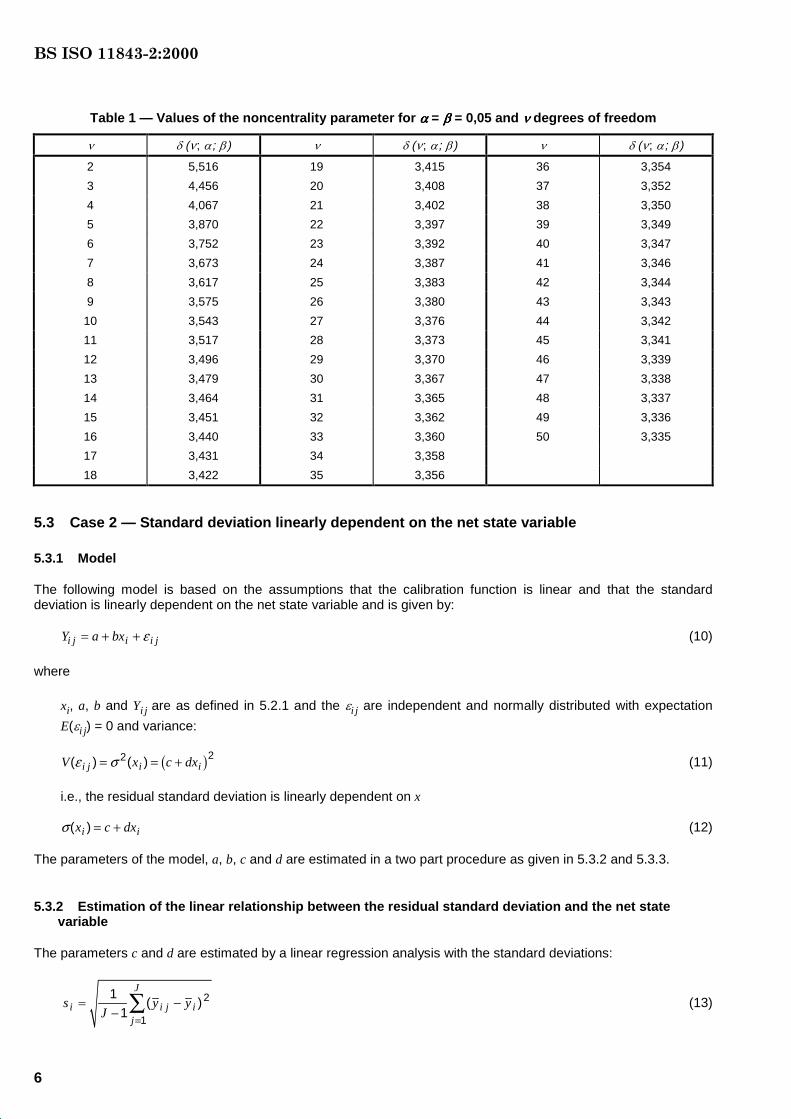
Table 1 presents �(� ; � ; �) for � = � = 0,05 and various values of �.

For � = � and � � 3, xd is approximated by

2

d 0,95 cˆ 1 1

2 ( ) 2ˆ xx

xx t x

K I J sb

��� � � �

�

(9)

BS ISO 11843-2:2000

6

Table 1 — Values of the noncentrality parameter for ���� = ���� = 0,05 and ���� degrees of freedom

� � (� ; � ; � ) � � (� ; � ; � ) � � (� ; � ; � )

2 5,516 19 3,415 36 3,354

3 4,456 20 3,408 37 3,352

4 4,067 21 3,402 38 3,350

5 3,870 22 3,397 39 3,349

6 3,752 23 3,392 40 3,347

7 3,673 24 3,387 41 3,346

8 3,617 25 3,383 42 3,344

9 3,575 26 3,380 43 3,343

10 3,543 27 3,376 44 3,342

11 3,517 28 3,373 45 3,341

12 3,496 29 3,370 46 3,339

13 3,479 30 3,367 47 3,338

14 3,464 31 3,365 48 3,337

15 3,451 32 3,362 49 3,336

16 3,440 33 3,360 50 3,335

17 3,431 34 3,358

18 3,422 35 3,356

5.3 Case 2 — Standard deviation linearly dependent on the net state variable

5.3.1 Model

The following model is based on the assumptions that the calibration function is linear and that the standarddeviation is linearly dependent on the net state variable and is given by:

Y a bxi j i i j� � � � (10)

where

xi, a, b and Yi j are as defined in 5.2.1 and the �i j are independent and normally distributed with expectation

E(�i j) = 0 and variance:

V x c dxi j i i( ) ( )� �� � �2 2

b g (11)

i.e., the residual standard deviation is linearly dependent on x

�( )x c dxi i� � (12)

The parameters of the model, a, b, c and d are estimated in a two part procedure as given in 5.3.2 and 5.3.3.

5.3.2 Estimation of the linear relationship between the residual standard deviation and the net statevariable

The parameters c and d are estimated by a linear regression analysis with the standard deviations:

2

1

1( )

1

J

i i j ij

s y yJ

�

� �

�

� (13)

BS ISO 11843-2:2000

7

as values of the dependent variable S and with the net state variable x as the independent variable. Since thevariance V(S) is proportional to �2, a weighted regression analysis (see references [1] and [2] of the Bibliography)has to be performed with the weights:

2 2

1 1

( ) ( )i

i i

wx c dx�

� �

�

(14)

However, the variances �2(xi) depend on the unknown parameters c and d that have yet to be estimated.Therefore, the following iteration procedure with weights:

�

( � )wqi

qi

�1

2�(15)

is proposed. At the first iteration, (q = 0), �� 0i = si, where the si values are the empirical standard deviations. Forsuccessive iterations q = 1,2, ...

� � �� qi q q ic d x� � (16)

calculate with the auxiliary values:

T wq qii

I

�

�

��111

, � ;

T w xq qi ii

I

�

�

��121

, � ;

T w xq qi ii

I

�

�

��132

1, � ; (17)

T w sq qi ii

I

�

�

��141

, � ;

T w x sq qi i ii

I

�

�

��151

, �

and

�, , , ,

, , ,

cT T T T

T T Tq

q q q q

q q q�

� � � �

� � �

�

�

�1

13 14 12 15

11 13 122

(18)

and

� , , , ,

, , ,

dT T T T

T T Tq

q q q q

q q q�

� � � �

� � �

�

�

�

111 15 12 14

11 13 122

(19)

This procedures converges rapidly so that the result for q = 3;

� � �� 3 3 3� �c d x ;

BS ISO 11843-2:2000

8

can be considered, with � � ( ), � �� � �3 3� �x c 0 and � �d d3 � , as the final result:

� ( ) � �� �x � �0 (20)

5.3.3 Estimation of the calibration function

The parameters a and b are estimated by a weighted linear regression analysis (see references [1] and [2] in theBibliography) with the yi j as values of the dependent variable, xi as values of the independent variable andweights:

wx

ii

�

12

� ( )�

;

where

� ( )�2 xi is the predicted value of the variance at xi according to equation (20)

with:

T J wii

I

11

�

�

� ;

T J w xii

I

i21

�

�

� ;

T J w xii

I

i31

2�

�

� ;

; (21)

the estimates for a and b are:

3 4 2 52

1 3 2

ˆT T T T

aT T T

�

�

�

(22)

�bT T T T

T T T�

�

�

1 5 2 4

1 3 22

(23)

5.3.4 Computation of critical values

The critical value of the response variable is given by:

y a tK T

x

sw

xxwc � � � �

F

HG

I

KJ� ( )

��,0 95

02

1

221

�

�

� (24)

dxˆ ‰

41 1

I J

i iji j

T w y= =

= ∑∑

51 1

I J

i i iji j

T w x y= =

= ∑∑

ˆ

‰

BS ISO 11843-2:2000

9

and the critical value of the net state variable is given by:

xt

b K T

x

sw

xxwc � � �

F

HG

I

KJ

0 95 02

1

221, ( )

�

��

� �

� (25)

where

x T Tw � 2 1/ (26)

s T T Txxw � �3 22

1/ (27)

� � ��2 2

11

12

�

� �

� �

��

��I Jw y a bxi i j i

j

J

i

I

e j (28)

and t0,95(�) is the 95 %-quantile of the t-distribution with � = I�J � 2 degrees of freedom; sxxw is defined in annex A.

5.3.5 Computation of the minimum detectable value

The minimum detectable value is given by:

xb

x

K T

x

sw

xxwd

d� � �

F

HG

I

KJ

� ��

�

� ( )�

2

1

221

(29)

where

� = � (� ; � ; �) is the value of the noncentrality parameter as defined in 5.2.4.

Since � ( )�2 xd depends on the value of xd yet to be calculated, xd has to be calculated iteratively.

The iteration starts with � ( ) �� �xd 0 0� and results in xd0; for the next iteration step d 1 d0ˆ ˆ( ) ( )x x� �� is computed and

used in the formula for xd, resulting in xd1,... In many cases even the first iteration step does not change the value

of xd appreciably; an acceptable value for xd is obtained at the third iteration step.

6 Minimum detectable value of the measurement method

The minimum detectable value obtained from a particular calibration shows the capability of the calibratedmeasurement process for the respective measurement series to detect the value of the net state variable of anobserved actual state to be different from zero, i.e. it is the smallest value of the net state variable which can bedetected with a probability of 1 � � as different from zero. This minimum detectable value differs for differentcalibrations. The minimum detectable values of different measurement series for

� a particular measurement process based on the same type of measurement process,

� a type of measurement process based on the same measurement method, or

� a measurement method

can be interpreted as realizations of a random variable for which the parameters of the probability distribution canbe considered characteristics of the measurement process, the type of measurement process or of themeasurement method, respectively.

BS ISO 11843-2:2000

10

If, for a particular measurement process, m consecutive calibrations have been carried out in order to determine theminimum detectable value of the net state variable xd, the m minimum detectable values xd1, xd2, ... xdm, can beused to determine a minimum detectable value of the measurement process under the following conditions:

a) the measurement process is not changed;

b) the distribution of the values xd is unimodal and there are no outlying values xd;

c) the experimental design (including the number of reference states, I, and the numbers of replications ofprocedure, J, K and L) was identical for each of the calibrations.

Under these conditions the median of the values xdi, for i = 1, ..., m, is recommended as the minimum detectablevalue of the measurement process; if another summary statistic of the values xdi is used instead of the median, thestatistic used shall be reported.

If any of these conditions are violated, the minimum detectable value of the measurement process is not sufficientlywell-defined and the determination of a common value shall not be attempted.

If the same measurement method is applied in p laboratories and for each of them a minimum detectable value ofthe measurement process within the laboratory were to be determined, then under the same conditions as for thedetermination of the minimum detectable value of the measurement process, the median of the p minimumdetectable values of the laboratories is recommended as the minimum detectable value of the measurementmethod; if another summary statistic of the minimum detectable values of the laboratories is used instead of themedian, the statistic used shall be reported.

7 Reporting and use of results

NOTE Examples of the determination of critical and minimal detectable values are given in annex C.

7.1 Critical values

For decisions regarding the investigation of actual states only the critical value of the net state variable or of theresponse variable is to be applied. These values derived from a calibration of the measurement process aredecision limits to be used to assess the unknown states of systems included in this series. Looking at consecutivecalibrations of the same measurement process, the critical values may vary from one calibration to another.However, since each of the critical values is a decision limit belonging to a particular measurement series, it ismeaningless to calculate overall critical values across calibrations and logically inappropriate to use these ascritical values.

If a value of the net state variable or of the response variable is not greater than the critical value, it can be statedthat no difference can be shown between the observed actual state and the basic state. However, due to thepossibility of committing an error of the second kind, this value should not be construed as demonstrating that theobserved system definitely is in its basic state. Therefore, reporting such a result as “zero” or as “smaller than theminimum detectable value” is not permissible. The value (and its uncertainty) should always be reported; if it doesnot exceed the critical value, the comment “not detected” should be added.

7.2 Minimum detectable values

The minimum detectable value derived from a particular calibration shows whether the capability of detection of theactual measurement process is sufficient for the intended purpose. If it is not, the number J, K or L may bemodified.

A minimum detectable value derived from a set of calibrations following the conditions mentioned in clause 6 mayserve for the comparison, the choice or the judgement of different laboratories or methods, respectively.

BS ISO 11843-2:2000

11

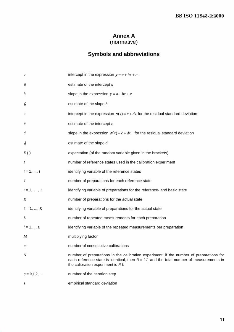
Annex A(normative)

Symbols and abbreviations

a intercept in the expression y a bx� � � �

�a estimate of the intercept a

b slope in the expression y a bx� � � �

�b estimate of the slope b

c intercept in the expression �( )x c dx� � for the residual standard deviation

�c estimate of the intercept c

d slope in the expression �( )x c dx� � for the residual standard deviation

�d estimate of the slope d

E ( ) expectation (of the random variable given in the brackets)

I number of reference states used in the calibration experiment

i = 1, ..., I identifying variable of the reference states

J number of preparations for each reference state

j = 1, ...., J identifying variable of preparations for the reference- and basic state

K number of preparations for the actual state

k = 1, ..., K identifying variable of preparations for the actual state

L number of repeated measurements for each preparation

l = 1,..., L identifying variable of the repeated measurements per preparation

M multiplying factor

m number of consecutive calibrations

N number of preparations in the calibration experiment; if the number of preparations foreach reference state is identical, then N = I�J, and the total number of measurements inthe calibration experiment is N�L

q = 0,1,2, ... number of the iteration step

s empirical standard deviation

BS ISO 11843-2:2000

12

s J x xxx ii

I

� �

�

�( )2

1

sum of squared deviations of the chosen values of the net state variable for the referencestates (including the basic state) from the average

s J w x xxxw i i wi

I

� �

�

� ( )2

1

weighted sum of squared deviations of the chosen values of the net state variable for thereference states (including the basic state) from the weighted average

T auxiliary value for the weighted linear regression analysis

V ( ) variance (of the random variable given in the brackets)

wi weight at xi

�wqi weight at xi in the qth iteration step

X net state variable, X = Z�� z0

x a particular value of the net state variable

x1, ..., xI chosen values of the net state variable X for the reference states including the basic state

xc critical value of the net state variable

xd minimum detectable value of the net state variable

xI

xii

I

�

�

�1

1

average of the chosen values of the net state variable for the reference states (includingthe basic state)

��

�x

y a

ba

�

�

estimated value of the net state variable for a specific actual state

x w x ww i ii

I

ii

I

�

� �

� �1 1

weighted average of the chosen values of the net state variable for the reference states(including the basic state)

Y response variable

yc critical value of the response variable

yi j l lth measurement of the jth preparation of the ith reference state

yk1, ..., yk l obtained values of the response variable for the kth preparation of a specific actual statein the measurement series

yK L

ya kll

L

k

K

�

�

��

��1

11

average of the observed values for a specific actual state

yI J L

yi j ll

L

j

J

i

I

�

� �

���

���1

111

average of the measurement values yi jl

yL

yi j i j ll

L

�

�

�1

1average of the measurement values of the jth preparation of the ith reference state

BS ISO 11843-2:2000

13

yJ L

yi i j ll

L

j

J

�

�

��

��1

11

average of the measurement values of the ith reference state

y0 average of the K� L measurement values at x = 0

Z state variable

z0 value of the state variable in the basic state

� probability of erroneously rejecting the null hypothesis "the state under consideration isnot different from the basic state with respect to the state variable" for each of theobserved actual states in the measurement series for which this null hypothesis is true(probability of the error of the first kind)

in the absence of specific recommendations the value � should be fixed at � = 0,05

� probability of erroneously accepting the null hypothesis “the state under consideration isnot different from the basic state with respect to the state variable” for each of theobserved actual states in the measurement series for which the net state variable isequal to the minimum detectable value to be determined (probability of the error of thesecond kind)

in the absence of specific recommendations the value � should be fixed at � = 0,05

� non-centrality parameter of the non-central t-distribution

� component of the response variable measurement representing the random componentof sampling, preparation and measurement errors

� degrees of freedom

� diff standard deviation of the difference between the average, y , and the estimated intercept,�a

�� estimate of the residual standard deviation

�� qi standard deviation at xi in the qth iteration step

�� 0 estimate of the residual standard deviation, x = 0

BS ISO 11843-2:2000

14

Annex B(informative)

Derivation of formulae

B.1 Case 1 — Constant standard deviation

Under the assumptions of 5.1 and in the case of constant standard deviation, estimations of the regressioncoefficients, �a and �b , are normally distributed with expectations

E a a E b b� ; �b g e j� �

and variances:

V aI J

x

sV b

sxx xx� ; �b g e j�

�

�

FHG

IKJ

�1 2

22

��

where

�2 is the variance of the residuals of the averages of the L repeated measurements for each preparation.

If the response variable is measured K�L times at the basic state z z x� �0 0,b g , the difference between the average

0y of the K�L values and the estimated intercept �a follows a normal distribution with expectation:

� � � � � �0 0ˆ ˆ 0E y a E y E a a a� � � � � �

and variance:

� � � � � �2 2 2

2 20 0

1 1 1ˆ ˆ

xx xx

x xV y a V y V a

K I J s K I J s

�� �

� � � �� � � � � � � � �� � � �� �

Since y a0 � �b g is normally distributed, the random variable

Uy a

�

�0 �

� diff

follows the standardized normal distribution, and the inequality:

y au0

0 95� �

,� diff

u

holds with probability 0,95. Since � diff2 is unknown it can be estimated as:

� �� �diff2

221 1

� �

�

�

F

HG

I

KJK I J

x

sxx

BS ISO 11843-2:2000

15

where

��2 is the estimated residual variance of the regression analysis that shall be used instead. The random

variable

Ty a

�

�

a f ��0 �

� diff

follows the t-distribution with � � � �I J 2 degrees of freedom, and the inequality:

y at00 95

� �

�( ),

�

�

diffu

or

y a t a tK I J

x

sxx0 0 95 0 95

21 1u � ( ) � � ( ) �, ,� � � �

�

�� � � �diff

where

t0 95, ( )� is the 95 %-quantile of the t-distribution with � degrees of freedom, holds with probability 0,95.

The right hand side of this inequality is the critical value of the response variable.

y a tK I J

x

sxxc � � �

�

�� ( ) �,0 95

21 1� �

and the critical value of the net state variable is

xy a

bt

b K I J

x

sxxc

c�

�� �

�

�

�

�( )

�

�,0 95

21 1�

�

Similar expressions describe these values when other quantiles of the t-distribution are appropriate.

In order to determine the minimum detectable value xd of the net state variable, it is necessary to examine the

distribution of y a� � �b g � diff in the case where the true value x of the net state variable is identical to the minimum

detectable value xd of the net state variable, x = xd. It is required to detect this state with probability 1� � , i.e:

Py a

t x x�

� �

L

NM

O

QP � �

�

�( ),

�� �

diffd0 95 1

or

Py a

t x x�

�

L

NM

O

QP �

�

�( ),

�� �

diffdu 0 95

If x = xd, the expectation of y is:

E y a bxa f � � d

BS ISO 11843-2:2000

16

and therefore:

E y a bx� ��b g d

whereas:

V y a� ��b g � diff2

as for x = 0.

Py a

t x x�

�

L

NM

O

QP

�

�( ),

�

�

diffdu 0 95

�

� � �

�

L

NM

O

QPP

y a bx bxt x x

�

�( ),

b g d d

diffd

�

�u 0 95

�

� ��

L

N

MMMM

O

Q

PPPP

P

y a bx bx

t

�

�( ),

d

diff

d

diff

diff diff

� �

� �

�u 0 95

��

L

N

MM

O

Q

PP

PU

t�

� � ��

20 95

( )( ),u

� P T t( ; ) ( ),� � �u 0 95 ;

since U� � �y a bx� /d diffb g � follows the standardized normal distribution and �� �diff diff independent of U follows

the distribution of � � �2( ) , the random variable T( ; )� � follows the noncentral t-distribution with � degrees of

freedom and noncentrality parameter �; � � � � �� ; ;b g for � � 0 05, or other appropriate value, if required is

determined as the value of the noncentrality parameter of the noncentral t-distribution with � degrees of freedomthat satisfies:

P T t( ; ) ( )� � � ��

u 1� �

From:

��

�

bxd

diff

the expression:

xb b K I J

x

sxxd

diff� � �

�

���

�� 1 1 2

for the minimum detectable value of the net state variable follows.

BS ISO 11843-2:2000

17

For a prognosis, the estimates of b and � are inserted into the formula so that the minimum detectable value isgiven by:

��

�x

b K I J

x

sxxd � �

�

��� 1 1 2

The critical value of the response variable yc is the sum of �a and a multiple of �� , and the critical value of the net

state variable is a multiple of � �� b. If, according to the recommendations, the values of the net state variable of thereference states are equidistantly spaced with the smallest value zero, � = 0,05 and either

� K = 1 (one preparation for the measurement of the actual state) or;

� K = J (number of preparations for the measurement of the actual state equal to this for the reference states);

the multiplier:

M tK I J

x

sxx� �

�

�0 95

21 1, ( )�

in the expressions for the critical values is a function of the number of reference states, I, and the number ofpreparations of each reference state, J, only. For some cases M is given in Table B.1.

Table B.1 — Determination of the multiplier factor, M

For K = 1

I J I�J 11 2

�

�

�

I J

x

sxxt0 95, ( )� M

3 1 3 1,35 6,31 8,52

3 2 6 1,19 2,13 2,54

5 1 5 1,26 2,35 2,97

5 2 10 1,14 1,86 2,12

5 4 20 1,07 1,73 1,86

For K = J

I J I�JI

I J

x

sxx

�

�

�1 2

t0 95, ( )� M

3 1 3 1,35 6,31 8,54

3 2 6 0,96 2,13 2,04

5 1 5 1,26 2,35 2,97

5 2 10 0,89 1,86 1,66

5 4 20 0,63 1,73 1,09

BS ISO 11843-2:2000

18

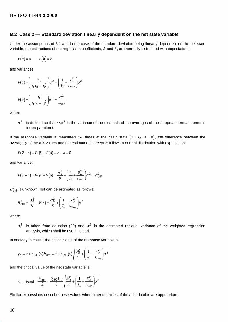
B.2 Case 2 — Standard deviation linearly dependent on the net state variable

Under the assumptions of 5.1 and in the case of the standard deviation being linearly dependent on the net statevariable, the estimations of the regression coefficients, �a and �b , are normally distributed with expectations:

E a a�b g � ; E b b�e j �

and variances:

V aT

T T T T

x

sw

xxw�b g �

�

F

HG

I

KJ � �

F

HG

I

KJ

3

1 3 22

2

1

221

� �

V bT

T T T sxxw

�e j ��

FHG

IKJ

�1

1 3 22

22

��

where

�2 is defined so that wi�

2 is the variance of the residuals of the averages of the L repeated measurementsfor preparation i.

If the response variable is measured K�L times at the basic state Z z X� �0 0,b g , the difference between the

average y of the K�L values and the estimated intercept �a follows a normal distribution with expectation:

E y a E y E a a a� � � � � �� �b g a f b g 0

and variance:

V y a V y V aK T

x

sw

xxw� � � � � �

F

HG

I

KJ �� �b g a f b g

�

� �02

1

22 21

diff

� diff2 is unknown, but can be estimated as follows:

��

� ��

��

� �

�diff2 0

202

1

221

� � � � �

F

HG

I

KJK

V aK T

x

sw

xxwb g

where

�� 02 is taken from equation (20) and ��

2 is the estimated residual variance of the weighted regressionanalysis, which shall be used instead.

In analogy to case 1 the critical value of the response variable is:

y a t a tK T

x

sw

xxwc diff� � � � � �

F

HG

I

KJ� ( ) � � ( )

��, ,0 95 0 95

02

1

221

� � �

�

�

and the critical value of the net state variable is:

x tb

t

b K T

x

sw

xxwc

diff� � � �

F

HG

I

KJ0 95

0 95 02

1

221

,,( )

�

�

( )�

���

� � �

�

Similar expressions describe these values when other quantiles of the t-distribution are appropriate.

BS ISO 11843-2:2000

19

These formulae include the case of constant standard deviation for which all the weights are equal to one, wi � 1

for i I� 1,..., so that T I J1 � � , x xw � , s sxxw xx� and � �� �02 2� .

The minimum detectable value of the net state variable is:

xbddiff

� ��

where, for x = xd,

� diff, d ddx V y a x x V y x x V a2� � � � � �� �c h c h b g

For a prognosis, the estimates of b and � diff, dx2 , �b and:

� � � �� diff, ddx V y x x V a2� � �c h b g� � �

F

HG

I

KJ

��

�

�

2

1

221x

K T

x

sw

xxw

db g

are inserted into the formula so that the minimum detectable value of the net state variable is given by:

xb

x

K T

x

sw

xxwd

d� � �

F

HG

I

KJ

� ��

�

��

2

1

221b g

Since ��2 xdb g depends on the value of xd yet to be calculated the iterative procedure of 5.3.5 has to be used.

BS ISO 11843-2:2000

20

Annex C(informative)

Examples

C.1 Example 1

The mercury content, expressed in ng/g1) of plant materials, was measured by atomic absorption spectroscopy.Each sample was decomposed using a microwave (MLS-1200) technique and taken up in nitric acid / potassiumdichromate solution. These solutions were examined through a Varian VGA-76 cold vapour reduction systemleading to a gold-plated foil concentration system (MCA-90) prior to replicated atomic absorption measurements. Inorder to estimate the calibration function and to determine the capability of detection, each of six reference samplesrepresenting the blank concentration (x = 0) and the net concentrations x = 0,2 ng/g; 0,5 ng/g; 1,0 ng/g; 2,0 ng/g;3,0 ng/g was prepared three times and each prepared sample measured once. Hence, I = 6; J = 3; L = 1.

It was assumed that the assumptions of linearity of the calibration function, constant standard deviation and normaldistribution of the response variable hold; � and � had been fixed in advance at � �� � 0 05, . For the determinationof the concentration of mercury in the material to be analysed, two different approaches were taken intoconsideration:

a) one measurement would be carried out (K = L = 1); or

b) three samples would be prepared for measurement and each of them measured once (K = 3; L = 1) and theaverage ya of the observed values used as the measurement result.

The results of the calibration experiment are given in Table C.1.

Table C.1 — Results of the calibration experiment for the determination of mercury contentin food or drugs

Referencesample

Net concentration ofmercury

Absorbance

i xi

ng/gyi j

1 0 0,003 � 0,001 0,002

2 0,2 0,004 0,005 0,005

3 0,5 0,011 0,011 0,012

4 1,0 0,023 0,023 0,023

5 2,0 0,048 0,047 0,048

6 3,0 0,071 0,072 0,072

1) 1 part per billion (ppb) = 10�9 g/g = 1 ng/g. The use of ppb is deprecated.

BS ISO 11843-2:2000

21

The statistical analysis yields:

x � 1116 7, ng/g

sxx � 20 425,

� ,a � ��9 995 9 10 5

� ,b � 0 023 74

� ,� � ��1109 9 10 3

Since � = N � 2 = 16;

t t0 95 0 95 16) 1746, ,( ) ( ,� � � ;

� � � � �( ; ; ) ( ; , ; , ,� �16 0 05 0 05) 3 440;

2 0,95t ( ) ,� � 3 492d i

The results for the approach a) are

critical value of the response variable [see equation (5)]

critical value of the net concentration [see equation (6)] xc ng /g� 0 086,

d ng/g� 0173,

� the smallest absorbance value which can be interpreted as coming from a sample with a net mercuryconcentration larger than the blank concentration is yc , the critical value of the responsevariable;

� the smallest net concentration of mercury in a sample which can be distinguished (with a probability of1 0 95� �� , ) from the blank concentration is xd ng/g� 0173, , the minimum detectable value of the netconcentration.

The results for approach b) are:

critical value of the response variable [see equation (5)]

critical value of the net concentration [see equation (6)] xc ng / g� 0 055,

minimum detectable net concentration xd ng / g� 0110,

C.2 Example 22)

The amount of toluene in 100 �l of extracts was measured using gas chromatography interfaced with a massspectrometric detector (GC/MS). 100 �l samples were injected into the GC/MS system. Six reference sampleswere used and contained toluene in known amounts in the range 4,6 pg/100 �l to 15 000 pg/100 �l. Each samplewas injected and measured four times (I = 6, J = 4, L = 1, N = 24). The measurement results are given in Table C.2.

2) D.M. ROCKE and S. LORENZATO. A Two-Component Model for Measurement Error in Analytical Chemistry. Technometrics,1995, 37, pp. 181-182.

c 0,002 15y =ˆ ‰

� 0,00 2 15ˆ ‰

minimum detectable net concentration [see equation (9)] xˆ ‰

[see equation (9)] ˆ ‰

c 0,001 40y =ˆ ‰

BS ISO 11843-2:2000

22

A look at the graphical representation of the measurement results shows that the relationship between the tolueneamount and the response variable (peak area) is satisfactorily linear; the standard deviation of the peak area islinearly dependent on the amount of toluene. Under the additional assumption of normal distribution of theresponse variable the capability of detection can be determined according to 5.3.

Table C.2 — Results of the calibration experiment for the toluene amount in 100 ����l extract

(1) (2) (3) (4) (5) (6) (7)

Referencesample

Net amountof toluene Peak area

Empiricalstandarddeviation

Predicted standard deviation ofiteration

1 2 3

i xi

pg/100 �l

yi j si �� 1 i �� 2i �� 3i

1 4,6 29,80 16,85 16,68 19,52 6,20 4,56 5,17 5,15

2 23 44,60 48,13 42,27 34,78 5,65 7,07 7,93 7,92

3 116 207,70 222,40 172,88 207,51 21,02 19,73 21,87 21,88

4 580 894,67 821,30 773,40 936,93 73,19 82,91 91,43 91,57

5 3 000 5 350,65 4 942,63 4 315,79 3 879,28 652,98 412,46 454,22 455,02

6 15 000 20 718,14 24 781,61 22 405,76 24 863,91 2 005,02 2 046,54 2 253,14 2 257,23

In the estimation procedure for c and d an iteratively reweighted linear regression analysis according to 5.3.2 iscarried out which produces the following estimated linear regression functions:

iteration 1: � , ,�1 3 933 23 0136 174i ix� �

iteration 2: � , ,� 2 4 482 84 0149 911i ix� �

iteration 3: � , ,� 3 4 462 28 0150 185i ix� �

The corresponding predicted standard deviations are given in columns (5) to (7) of Table C.2. After the thirditeration the results are stable so that the equation of iteration 3 can be used as the final result of part 1 of theestimation procedure, i.e.:

� ( ) , ,� x x� �4 462 28 0150 185

� ,� 0 4 462 28�

The parameters a and b of the calibration function are estimated by a weighted linear regression analysis accordingto clause 5.3.3 with the yi j of column (3) as values of the dependent variable, xi of column (2) as values of theindependent variable and weights:

wx x

ii i

� �

�

1 1

4 462 28 0150 1852 2� , ,� b g b g

This regression analysis yields:

T J wii

I

11

�

�

� = 0,223 306

xw = 15,566 9

BS ISO 11843-2:2000

23

sxxw = 606,224

�a = 12,218 5

�b = 1,527 27

��2 = 1,059 54

� = N � 2 = 22

t0 95, �a f = t0 95 22, a f = 1,717

Therefore for K = 1, the following are obtained:

critical value of the response variable [see equation (24)] yc � 20 82,

the critical value of the net toluene amount in 100 �l of extract [see equation (25)] xc � 5 63, pg.

The minimum detectable value is calculated iteratively:

For � �� � 0 05, , � � � � �; ; ; , ; , ,b g b g� �22 0 05 0 05 3 397(see Table 1) and with � �� �xdb g0 0� the first value for xd

[see equation (29)] is xd0 = 11,139; it follows � ,� xdb g1 6135 2� and xd1 14 553� , ;

with � ,� xdb g2 6 647 9� iteration 2 leads xd2 15 627� , pg/100 �l and

with � ,� xdb g3 6 809 2� we get finally x xd d3� � 15 967, pg/100 �l.

The smallest peak area which can be interpreted as coming from a sample with a net toluene concentration largerthan the blank concentration is yc � 20 82, , the critical value of the response variable.

The smallest net amount of toluene in a sample of 100 �l extract which can be distinguished (with a probability of1 0 95� �� , ) from the blank concentration is xd ,� 15 97 pg/100 �l, the minimum detectable value of the net tolueneconcentration.

BS ISO 11843-2:2000

24

Bibliography

[1] DRAPER N.R. and SMITH H. Applied Regression Analysis. Wiley, New York, 1981.

[2] MONTGOMERY D.C. and PECK E.A. Introduction to Linear Regression Analysis. Wiley, New York, 1992.

[3] CURRIE L.A. Nomenclature in Evaluation of Analytical Methods Including Detection and QualificationCapabilities. IUPAC Recommendations 1995. Pure and Applied Chemistry, 67, 1995, pp. 1699-1723.

BS ISO 11843-2:2000

blank

BS ISO 11843-2:2000

BSI389 Chiswick High RoadLondonW4 4AL

BSI — British Standards InstitutionBSI is the independent national body responsible for preparing British Standards. It presents the UK view on standards in Europe and at the international level. It is incorporated by Royal Charter.

Revisions

British Standards are updated by amendment or revision. Users of British Standards should make sure that they possess the latest amendments or editions.

It is the constant aim of BSI to improve the quality of our products and services. We would be grateful if anyone finding an inaccuracy or ambiguity while using this British Standard would inform the Secretary of the technical committee responsible, the identity of which can be found on the inside front cover. Tel: +44 (0)20 8996 9000. Fax: +44 (0)20 8996 7400.

BSI offers members an individual updating service called PLUS which ensures that subscribers automatically receive the latest editions of standards.

Buying standards

Orders for all BSI, international and foreign standards publications should be addressed to Customer Services. Tel: +44 (0)20 8996 9001. Fax: +44 (0)20 8996 7001. Email: orders@bsi-global.com. Standards are also available from the BSI website at http://www.bsi-global.com.

In response to orders for international standards, it is BSI policy to supply the BSI implementation of those that have been published as British Standards, unless otherwise requested.

Information on standards

BSI provides a wide range of information on national, European and international standards through its Library and its Technical Help to Exporters Service. Various BSI electronic information services are also available which give details on all its products and services. Contact the Information Centre. Tel: +44 (0)20 8996 7111. Fax: +44 (0)20 8996 7048. Email: info@bsi-global.com.

Subscribing members of BSI are kept up to date with standards developments and receive substantial discounts on the purchase price of standards. For details of these and other benefits contact Membership Administration. Tel: +44 (0)20 8996 7002. Fax: +44 (0)20 8996 7001. Email: membership@bsi-global.com.

Information regarding online access to British Standards via British Standards Online can be found at http://www.bsi-global.com/bsonline.

Further information about BSI is available on the BSI website at http://www.bsi-global.com.

Copyright

Copyright subsists in all BSI publications. BSI also holds the copyright, in the UK, of the publications of the international standardization bodies. Except as permitted under the Copyright, Designs and Patents Act 1988 no extract may be reproduced, stored in a retrieval system or transmitted in any form or by any means – electronic, photocopying, recording or otherwise – without prior written permission from BSI.

This does not preclude the free use, in the course of implementing the standard, of necessary details such as symbols, and size, type or grade designations. If these details are to be used for any other purpose than implementation then the prior written permission of BSI must be obtained.

Details and advice can be obtained from the Copyright & Licensing Manager. Tel: +44 (0)20 8996 7070. Fax: +44 (0)20 8996 7553. Email: copyright@bsi-global.com.