can compulsory military service raise civilian wages...

57

American Economic Journal: Applied Economics 2012, 4(4): 57–93 http://dx.doi.org/10.1257/app.4.4.57

Can Compulsory Military Service Raise Civilian Wages? Evidence from the Peacetime Draft in Portugal†

By David Card and Ana Rute Cardoso*

We provide new evidence on the long-term impacts of peacetime conscription, using longitudinal data for Portuguese men born in 1967. These men were inducted at age 21, allowing us to use pre-conscription wages to control for ability differences between con-scripts and nonconscripts. We find a significant 4–5 percentage point impact of service on the wages of men with only primary education, coupled with a zero effect for men with higher education. The effect for less-educated men suggests that mandatory service can be a valu-able experience for those who might otherwise spend their careers in low-level jobs. (JEL J24, J31, J45)

Throughout the twentieth century young men in most Western countries faced the risk of military conscription. Although compulsory service ended in the

United States in 1973, the practice continued until very recently in many European nations, and is still widely used around the world.1 Spurred in part by recent deci-sions to end conscription in Sweden, Italy, France, and Germany, there is renewed interest in understanding the impacts of mandatory service on a wide range of out-comes, including earnings (Angrist and Chen 2011; Angrist, Chen, and Song 2011; Grenet, Hart, and Roberts 2011; Paloyo 2010), education (Maurin and Xenogiani 2007; Cipollone and Rosolia 2007; Keller, Poutvaara, and Wagener 2010; Bauer et al. 2012), health (Bedard and Deschenes 2006; Dobkin and Shabani 2009; Autor, Duggan, and Lyle 2011), and crime (Galiani, Rossi, and Schargrodsky 2011).

Revealed preference arguments suggest that conscripts will suffer economic losses from coerced service (e.g., Oi 1967). Nevertheless, some analysts have argued that compulsory service can have a positive return for disadvantaged youth who face limited civilian job opportunities (e.g., Berger and Hirsch 1983; de Tray 1982).2 Seminal research by Angrist (1990) showed that Vietnam-era draftees had

1 In Europe, for example, Austria, Denmark, Estonia, Finland, Greece, Norway, and Switzerland all still require men to perform some form of national service. Russia and China also have mandatory military service.

2 Hirsh and Mehay (2003) studies wage differences between reservists who have served in active duty and those who have not, and find small average differences, but a positive impact of service for African Americans.

* Card: University of California, Berkeley, Department of Economics, 508-1 Evans Hall 3880, Berkeley, CA 94720-3880 and National Bureau of Economic Research (NBER) (e-mail: [email protected]); Cardoso: IAE-CSIC and Barcelona GSE; Campus UAB, 08193 Bellaterra, Barcelona, Spain (e-mail: [email protected]). We are grateful to two referees and to Joshua Angrist and Patrick Kline for helpful comments. We also thank the Statistics Department of the Portuguese Ministry of Employment for access to the data. This research was supported by the Center for Labor Economics at UC Berkeley. Cardoso also gratefully acknowledges support from the Spanish Ministry of Science and Innovation (grant ECO2009-07958), the Spanish Ministry of Education (mobility grant PR2010-0004), and the Government of Catalonia.

† To comment on this article in the online discussion forum, or to view additional materials, visit the article page at http://dx.doi.org/10.1257/app.4.4.57.

http://dx.doi.org/10.1257/app.4.4.57

mailto:[email protected]




58 AmEricAn Economic JournAL: APPLiEd Economics ocToBEr 2012

lower earnings than non-draftees, a finding he attributed to the low value of mili-tary experience in the civilian labor market. Subsequent research in the United States and other countries, however, has uncovered a surprisingly mixed pattern of impacts. Imbens and van der Klaauw (1995) found that 10 years after conscription Dutch veterans earned lower wages than those who avoided service. In contrast, Albrecht (1999) estimated a positive earnings premium for Swedish conscripts. Grenet, Hart, and Roberts (2011) finds no long-run impact on the wages of British conscripts; likewise, Bauer et al. (2012) finds no effect for West German con-scripts.3 In a recent re-analysis of the Vietnam-era draftees, Angrist and Chen (2011) finds that by age 50 they have about the same earnings as non-draftees, and slightly higher education.

In this paper, we present new evidence on the long-run effects of mandatory mili-tary service, using detailed longitudinal data for Portuguese men born in the late 1960s. Some 40 percent of the men in these cohorts served in the military; a major-ity entered the service with less than six years of formal schooling. Our analysis relies on a unique annual census of wages—the Quadros de Pessoal (QP)—that allows us to track the cohorts of interest from their initial entry into the labor market until their early 40s. Using the fact that employers were required to treat conscripted employees as being on leave of absence, we can identify men who were working just prior to the age of conscription (age 21) and then entered the military, and a comparison group of men who remained in civilian jobs over the same period.

Implementing a series of difference-in-differences estimators, we find that the average impact of military service for men who had entered the labor market by age 21 is positive but insignificantly different from zero throughout the period from 2 to 20 years after their service. This small average effect, however, masks a statisti-cally significant later-life impact of about 4–5 percent for men with lower levels of education (under six years of schooling), coupled with a zero effect for men with higher education. The positive impact for the less-educated group mirrors the find-ings for US veterans by Berger and Hirsch (1983) and suggests that mandatory service can be a valuable experience for disadvantaged men who might otherwise spend their careers in low-level jobs. Our confidence in these results is bolstered by three additional findings. First, we find that wages of the men who eventually served in the military and those who did not track each other very closely in the period up to age 21. Second, we find that pre-conscription wages are a strong predictor of wages 10 to 20 years later, suggesting that any differences in average ability between veter-ans and nonveterans are revealed by their wages in the period prior to conscription. Third, comparisons of employment rates show that the veterans converge to the non-veterans within about 6–7 years after the completion of service, alleviating concerns about possible selection biases.

While our primary focus is on the effect of conscription for men who were work-ing prior to age 21, an important concern is that conscription could have had dif-ferent effects on other groups—e.g., those who never worked prior to age 21. As a check, we relate average wages for men born in different years from 1959 to 1969

3 Kunze (2002) analyzes longitudinal data for German workers and finds a complex pattern of earnings premi-ums for veterans.

VoL. 4 no. 4 59cArd And cArdoso: PEAcETimE drAfT in PorTugAL

to cohort-level data on conscription rates. Consistent with our main findings, this analysis points to a small positive average effect of conscription, and rules out a large negative average effect across all the men in a particular cohort.

The next section of the paper provides a brief overview of the institutional back-ground underlying the conscription process in Portugal in the late 1980s. Section II discusses the QP dataset and our method for identifying conscripts, based on unpaid leave-of-absence status. We then provide a comparison of the conscript and non-conscript groups, as well as other individuals in the birth cohort under analysis. Section IV presents the details of our statistical approach, which takes advantage of the availability of pre-conscription earnings data to control for potential ability differ-ences between conscripts and nonconscripts. Section V presents our main findings, first using graphical techniques, then using more formal regression models, including models that explore a range of possible values for the relative effect of unobserved ability in pre-conscription versus post-conscription earnings. We also explore pos-sible mechanisms driving the enlistment effect. Section VI presents our inter-cohort comparisons for men born between 1959 and 1969, while Section VII concludes.

I. Military Service in Portugal

During the 1960s and early 1970s Portugal fought colonial wars in Angola, Mozambique, and Guinea-Bissau staffed by a far-reaching conscription system.4 Following the overthrow of the Estado Novo regime in 1974 and the withdrawal from Africa, the Portuguese military transitioned to a smaller peacetime force.5 Throughout the 1980s and early 1990s men were at risk of conscription in the year they turned 21, and draftees were required to serve for a maximum of two years.6 Individuals were called for medical and psychological evaluations in the year they turned 20. Those judged physically or mentally unfit and those convicted of serious felonies were exempted from service. A tiny fraction of men (some 100 to 300 per year) also met the substantial hurdles to qualify for alternative service as conscien-tious objectors (Domingues 1998). Short-term deferments could be granted to stu-dents and individuals who were the sole providers for their family, but options for self-selecting out of service altogether were quite limited.

Over the 1990s, a series of laws reduced the age of conscription to 20 (effec-tive in 1993 for men born in 1973 or later) and reduced the duration of service to a maximum of 8 months for the 1970 and 1971 birth cohorts, and to 4 months for those born in 1972 or later. Finally, in 2005, peacetime conscription ended and the Portuguese military became an all-volunteer force open to both men and women.

Table 1 presents a variety of data on the conscription system facing Portuguese men born from 1959 to 1979, including the size of each cohort, the age of determination

4 By the early 1970s, some 8 percent of the Portuguese labor force were in the military (Graham 1979). A relatively large number of young people—over 100,000 per year in 1970, for example—left the country illegally to avoid service (Baganha and Marques 2001, table 2.10).

5 Carrington and de Lima (1996) study the impact of the large number of retornados—Portuguese nationals who returned at the end of the colonial wars—on labor market conditions in Portugal.

6 Information on the terms of service for men who served in the 1980s and 1990s is taken directly from legal statutes. See the Appendix for a list of these laws.


of conscription status, the number of men drafted in the year the cohort reached the age of conscription, the fraction of the cohort who were conscripted, and their maxi-mum length of service. The conscription rate for men born in the 1960s and 1970s ranged from 30 to 50 percent, with a dip for the 1972 and 1973 cohorts who were both subject to the draft in 1993. Note that unlike the situation in some European countries, peacetime service in Portugal was far from universal. Instead, the fraction of men who served in a given cohort was determined by the manpower needs of the military, the duration of service, and the size of the cohort.

Once in the military, conscripts with the lowest levels of education could under-take basic skills training, while those with higher schooling could undertake occupa-tional training. Labor laws in Portugal specify that occupational training acquired in the military is equivalent to civilian training, allowing some conscripts to accumu-late transferable skills.7 Another important piece of legislation required employers to treat drafted men as “on leave” from their job. This provision may have discour-aged firms from hiring young men until their conscription status was settled, though, as we discuss below, we see no evidence of this behavior. For those who were hired

7 Currently, such equivalence is guaranteed for training in such fields as professional driving, cooking and bak-ery, and emergency medical support.

Table 1—Cohort Size, Age of Conscription, Conscription Rate, and Maximum Length of Service

Year of birth

Number of men in cohort (1000’s)

(1)

Age of conscription for cohort

(2)

Number of men conscripted (1000’s)

(3)

Percent of men conscripted

(4)

Maximum length of service

(months) (5)

1959 109.7 21 35.5 32.4 241960 110.5 21 33.1 30.0 241961 111.9 21 30.7 27.5 241962 113.8 21 34.2 30.0 241963 109.5 21 39.1 35.7 241964 112.4 21 38.3 34.1 241965 108.6 21 36.4 33.6 241966 107.2 21 36.8 34.3 241967 103.9 21 40.9 39.3 241968 101.1 21 39.3 38.8 241969 98.1 21 34.0 34.7 241970 89.2 21 41.9 46.9 81971 97.3 21 37.1 38.1 81972 90.3 21 41.9 23.4 41973 88.7 20 41974 88.1 20 40.0 45.4 41975 93.1 20 43.7 46.9 41976 96.6 20 36.6 37.9 41977 94.0 20 29.4 31.3 41978 87.1 20 29.2 33.6 41979 82.7 20 28.9 35.0 4

notes: Column 1 is number of men born in indicated year. Column 2 is legal age of conscription. Column 3 is number of men conscripted into the army in the year the cohort turned 21 (born 1972 or earlier) or 20 (born 1973 or later). Number conscripted excludes a small number of men conscripted into the airforce and navy. Men born in 1972 and 1973 were both conscripted in 1993, and entry in column 3 is total for both cohorts. Column 4 repre-sents the ratio of column 3 to column 1: for the cohorts born in 1972 and 1973 we assume equal conscription rates. Column 5 is the maximum length of service.

source: See data Appendix for sources


and subsequently drafted, however, it presumably eased the transition back to civil-ian life. Finally, conscripts in good standing could re-enlist for up to eight years of additional service, though re-enlistment rates were generally quite low.

II. Data on Earnings and Conscription Status

A. The Quadros de Pessoal

Our analysis relies on a unique administrative dataset, the Quadros de Pessoal (QP), collected annually by the Ministry of Employment. The QP is a census of paid workers in the Portuguese private sector. All firms with at least one paid worker are legally obligated to return information on their full roster of employees, including wages and hours of work during the appropriate reference week (in March until 1993 and in October since 1994).8 Importantly, for our purposes, during the 1980s and 1990s, the QP asked employers to include men on leave for military duty in their roster. We identify individuals with missing values for their earnings and hours of work in the reference week as being “on leave.” 9 A limitation of the data is that government workers—who comprise just under 20 percent of the Portuguese work-force—are excluded from coverage.10 A second limitation is that the QP provides only a snapshot of labor market outcomes in each year. Individuals who are unem-ployed or out of the labor force at the time of the census have no labor market data for that year. Electronic records from the QP are available for the period from 1986 to 2009, and include worker and firm identifiers that allow individuals to be tracked over time and across jobs. Worker-level data are unavailable for 1990 and 2001, creating gaps in the worker histories in those two years.

Information for employees in the QP includes gender, date of birth, current edu-cational attainment, occupation, date of hire, base earnings, supplemental payments, and hours of work. Information on the employer side includes industry and location of the firm, gross annual revenues, and ownership status. We use an edited version of the data that has been checked for consistency of the longitudinal matches (see the data Appendix). We measure a worker’s gross hourly wage by dividing the sum of the individual’s monthly base wage and other regularly paid benefits by his or her normal hours of work.11 All wages are deflated using the Consumer Price Index (2009 = 100). We treat as missing any wage observation that is below 0.75 of the first percentile of wages, or above three times the ninety-ninth percentile, in the

8 Firms are required to post their employee rosters and the corresponding salary information in a public place visible by its workers, helping to ensure the accuracy of the reported information. During the 1980s there was some undercoverage in the QP, particularly of small firms (Braguinsky, Branstetter, and Regateiro 2011).

9 Firms may also fail to report earnings and hours for other reasons, including long-term illnesses, strikes, and maternity leave—see Table A.1 in the online Appendix. Unfortunately, the reason for leave status is not available in the electronic version of the QP.

10 Also missing from the employee rosters are contract workers. In recent years, such workers have accounted for a growing share of employment (Rebelo 2003).

11 Reported earnings are net of the employer portion of social security taxes but include the employee portion of the tax, currently 11 percent during the period under analysis. For a fraction of workers the employer’s report of hours appears to depend on the number of days worked in the survey month, which varies from year to year. All our models include year effects to control for this variation.


corresponding year. This eliminates a small fraction (about 1 percent) of observa-tions that appear to reflect misplaced decimals and similar gross errors.

B. identifying conscripts

Ideally we could combine information from military records with labor market data from the QP to study the impacts of service on all veterans, including men with no record of employment prior to conscription. Unfortunately, individual military service records are not available. Thus, we have to infer conscription status from the observed data in the QP. We focus on men born before 1970 (when the maximum term of service was reduced to eight months), and make use of the fact that employ-ers were instructed to report workers who had been drafted as on leave. A compli-cation is that some of the conscripts in a given year could be inducted early in the year, before the March date of the QP, and others could be inducted after the QP was completed. We therefore identify two separate groups of conscripts: men who are recorded in the QP as working full time in March of the year they turned 20 years of age, and are “on leave” (i.e., reported with missing earnings and hours) in the next two years; and men who were working full time in March of the year they turned 21, and were on leave in March in the next year.12 As a comparison group we use men who were working full time in March of the year they turned 21 and in March of the following year. These men could not have been inducted into the military at age 21 and served more than a year. Note that we are limiting attention to conscripts and nonconscripts who were working just before or just after reaching the age of 21. This has the important advantage that we have a full-time wage observation for each person at (approximately) age 21. For conscripts, the wage is measured just prior to entering the military at age 20 or 21. For nonconscripts, it is measured in the year they turn 21.

To implement these definitions we need to limit attention to cohorts that reached the age of 20 in 1986 or later (the first year QP data are available). Moreover, since the QP has a gap in 1990, we cannot use data for cohorts born in 1968 or 1969, as their status in the years they turned 21 or 22 is unknown. Given these constraints, we focus on men born in 1967 as our primary cohort of interest. These men were 18 or 19 at the time of the first available QP survey in March 1986 and can be fol-lowed continuously for three years until the break in the data in 1990 (i.e., until March 1989, when they were 21 or 22 years of age). In particular for this cohort, we have at least two years of data on wages prior to the age at which their conscription status was determined.

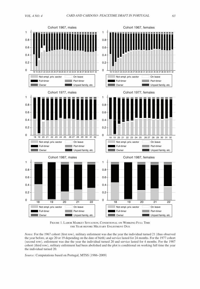
Before proceeding further it is important to verify that men born in 1967 who were working full time at age 20 or 21 and then recorded as on leave were actu-ally conscripted. While we cannot offer definitive proof, we conducted a series of comparisons summarized in Figure 1 that we believe are highly supportive of our assumptions. The upper left-hand panel of the figure shows the distribution

12 As a robustness check, we consider relaxing the criteria for the first subgroup slightly by requiring that they were employed full time in March of the year they turned 20 and on leave in the next March. We show this has very little effect on our results.


0

0.2

0.4

0.6

0.8

1

18 19 20 21 22 23 24 25 26 27 28 29 30 31 32 33 34 35 36 37 38 39 40 41 42

Cohort 1967, males Cohort 1967, females

18 19 20 21 22 23 24 25 26 27 28 29 30 31 32


18 19 20 21 22


Not empl. priv. sector On leave

Full-timer Part-timer

Owner Unpaid family, etc.

0

0.2

0.4

0.6

0.8

1

0

0.2

0.4

0.6

0.8

1

0

0.2

0.4

0.6

0.8

1

0

0.2

0.4

0.6

0.8

1

0

0.2

0.4

0.6

0.8

1

18 19 20 21 22 23 24 25 26 27 28 29 30 31 32 33 34 35 36 37 38 39 40 41 42

18 19 20 21 22
















18 19 20 21 22 23 24 25 26 27 28 29 30 31 32

Figure 1. Labor Market Situation, Conditional on Working Full Time the Year before Military Enlistment Due

notes: For the 1967 cohort (first row), military enlistment was due the year the individual turned 21 (thus observed the year before, at age 20 or 19 depending on the date of birth) and service lasted for 24 months. For the 1977 cohort (second row), enlistment was due the year the individual turned 20 and service lasted for 4 months. For the 1987 cohort (third row), military enlistment had been abolished and the plot is conditional on working full time the year the individual turned 20.

source: Computations based on Portugal, MTSS (1986–2009)


of activities in each year of age from 18 to 42 for men born in 1967 who were observed working full time at either age 20 or 21. Notice that the fraction of the cohort reported on leave is relatively high for only two years—ages 21 and 22. Moreover, the total fraction observed working or on leave at ages 21 and 22 is very similar to the fraction observed working at ages 23 and older. This pattern strongly suggests that leave of absence status is associated with military service. By comparison, the upper right-hand panel shows similar data for women born in 1967. For women there is no “unusual” spike in the fraction on leave at ages 21 and 22, confirming that the draft is the likely explanation for the high fraction of men on leave at these ages.

Comparisons with later cohorts of men and women, presented in the middle and lower panels of the figure, provide further evidence that most of the men from the 1967 cohort who were on leave at ages 21–22 were in the military. In the middle panels, we show data for people born in 1977 who were observed working full time at age 19 or 20. (We adjust the requirement on age to reflect the fact that conscrip-tion occurred at age 20 for this cohort). Consistent with the very short term of mili-tary service for this cohort (four months maximum), we see only a relatively small rise in the fraction of men classified as on leave at age 20. For women born in 1977 the patterns look very similar to those of women born 10 years earlier. Finally, in the lower panels of Figure 1, we show data for men and women born in 1987 who were observed working full time at age 19 or 20. For this cohort there was no mandatory military service, and reassuringly only a very small fraction of men are recorded as on leave between the ages of 20 and 22. Again, the data for women look relatively similar to the data for women born 10 or 20 years earlier.

While we believe that military service accounts for the unusual spike in the frac-tion of 1967 men on leave at ages 21 and 22, some men would obviously fall into this category even in the absence of conscription. To estimate the “false positive” rate, we tabulated the fractions of men at different ages who were working in the 1988 QP and on leave in 1989. This fraction was 19.0 percent for 21-year-olds, 9.0 percent for 22-year-olds, 3.0 percent for 23-year-olds, and between 2.7 percent and 3.0 percent for men between the ages of 24 and 30. Comparing 21-year-olds to those 23 and older, we infer that about 15 percent of 21-year-olds were probably on leave for other reasons. This means that simple comparisons between men identi-fied as conscripts, and those identified as nonconscripts, will likely understate the magnitude of the true gap by about 15 percent.

III. The 1967 Birth Cohort: Conscripts, Nonconscripts, and Others

While we can use employment and leave status information to identify a group of men born in 1967 who were working just before the determination of their conscription status and served in the military, and a comparison group who did not serve, there are many others in the cohort whose draft status is uncertain, including men with no record of employment by age 21. Table 2 presents some compara-tive information on the various subgroups to help contextualize our main groups of interest.

Out of the full cohort of approximately 104,000 men born in 1967 (see Table 1), approximately 90 percent are observed as private-sector employees in the QP at some


point between 1986 and 2009. Of these, about 5 percent have some inconsistency in their data (i.e., a missing or outlier wage observation if employed, or a problem link-ing records over time). Deletion of these observations leads to a sample of 86,909 men born in 1967 and ever observed in the QP with valid data, summarized in col-umn 1 of Table 2. Given the low schooling attainment of this cohort (mean com-pleted school at age 35 = 7 years) most of the men were presumably out of school by age 19. Nevertheless only about one-fifth were working full time at age 20 or 21 and meet the criteria to be potentially used in our analysis.13 Despite the relatively

13 A concern about the legal requirement that draftees be allowed to return to their job at the end of their service is that this would discourage employers from hiring men before the age of 21. We conducted a difference-in-differ-ences analysis of employment rates of men and women at ages 19 and 20 between cohorts born in 1967 and those born in 1987, testing whether the employment rates of the 1967 cohort of men were unusually low. This shows a small male × 1967 interaction effect (around − 1.5 percentage points), potentially indicating a small discourage-ment effect in the hiring of men when the draft was in effect.

Table 2—Summary Statistics on Sub-Groups of Male Cohort Born 1967

Fullcohort(1)

Early entrants (working full-time in 1987 or 1988)Not early

entrants(8)

Conscripted

Total(2)

Yes/no(3)

Yes(4)

No(5)

Missing(6)

Residual(7)

Number of observations 86,909 18,517 6,749 1,838 4,911 9,502 2,266 68,392Pre-conscription: Share w/observed wage 1986 14.1 46.6 51.4 62.1 47.4 39.9 61.0 5.3 1987 16.5 72.3 66.4 77.5 62.3 71.5 93.2 1.4 1988 15.5 68.0 95.0 81.5 100.0 58.9 25.7 1.2 1989 13.2 36.7 72.8 0.0 100.0 0.0 82.9 6.8 Share on leave absence 1986 0.5 1.1 1.2 1.0 1.3 1.0 1.4 0.4 1987 0.6 0.9 1.5 1.4 1.6 0.6 0.2 0.5 1988 2.1 6.0 5.0 18.5 0.0 3.3 19.8 1.1 1989 3.4 11.8 27.2 100.0 0.0 0.0 15.0 1.2 (Log) real hourly wage 1986 0.60 0.61 0.62 0.63 0.61 0.60 0.62 0.58 1987 0.78 0.78 0.79 0.80 0.78 0.77 0.78 0.78 1988 0.84 0.84 0.85 0.86 0.85 0.83 0.88 0.83 1989 0.91 0.92 0.92 0.92 0.93 0.90

Schooling: Share ≤ 4 years at entry 40.8 53.7 53.2 46.4 55.8 53.9 54.5 37.3 Av. at entry labor market 6.9 5.3 5.3 5.5 5.3 5.3 5.2 7.3 Av. in 2002 7.1 5.8 5.8 6.0 5.8 5.8 5.7 7.5

Post-conscription: Share w/wage obs, 02–09 60.9 62.2 72.6 72.4 72.7 52.4 72.0 60.6 (Log) real hr wage, 02–09 1.66 1.54 1.55 1.57 1.54 1.55 1.52 1.71

notes: Early entrants are defined as men who were observed working full time in either 1987 or 1988. Conscripted men include men who were working full time in 1987, and were on leave of absence (listed on the roster of employ-ees with missing values for wages and hours) in 1988 and 1989, plus men who were working full time in 1988 and on leave in 1989. Nonconscripted men are those who were working full time in 1988 and 1989. Missing group in column 6 are those who were working full time in 1987 or 1988 and are not present in the QP in 1989. Residual group in column 7 are all men who were working full time in 1987 or 1988 and are not included as conscripts, non-conscripts, or missing. Share with wage observation(s), 2002–2009 refers to the fraction of the group indicated in the column heading who were observed as wage earners in the QP at least once between 2002 and 2009.



low fraction working before age 21, the bottom rows of the table show that 61 per-cent are observed at least once between 2002 and 2009 (at ages 35–42).

Column 2 shows the characteristics of the entire sample of “early labor market entrants” (i.e., those who were working full time at age 20 or 21). Interestingly, the fraction of this subgroup observed in the QP at least once between 2002 and 2009 is very similar to the fraction of the entire cohort observed in that interval (62 percent versus 61 percent), while the average wages of the early labor market entrants are about 12 percent lower than the average wage for the entire cohort. We suspect that most of the difference is attributable to the relatively lower schooling of the early labor market entrants. By 2002, their average years of completed schooling was 5.8 years, versus 7.1 years for the cohort as a whole.

Among the early labor market entrants we identify four subgroups: conscripts (column 4 of Table 2), who were either working full time in March 1987 and on leave the next two years, or working full time in March 1988 and on leave the next year; nonconscripts (column 5), who were working full time in both March 1988 and March 1989; people missing from the QP in 1989 (column 6) who were pre-sumably unemployed, out of the labor force, or working in the government sector in March 1989; and finally, a fourth residual group (column 7) made up of men with a variety of employment histories in the period from 1987 to 1989 that do not fit into the other three groups. Both the missing and residual groups include a mix of conscripts and nonconscripts. For example, men who were working full time in March 1988 but subsequently left that job before entering the military later in the year would appear in the “missing” group.

Comparisons across columns 4–7 show that the 1986–1988 wages of the con-scripted and nonconscripted groups are quite similar, while the wages of the group who are missing from the 1989 QP are a little lower, and those of the residual group are a little higher. The conscripts have the highest education levels of the four groups of early entrants, measured either in the first year they ever appear in the QP, or in 2002. Anecdotal evidence suggests that the military generally preferred men with higher literacy and numeracy skills, leading to a systematic under-representation of the lowest educated men in the conscripted group. Nevertheless, conscripts and nonconscripts have nearly the same probability of appearing in the QP in the period from 2002 to 2009, and fairly similar hourly wages. Interestingly, the group that was missing from the QP in 1989 has a much lower likelihood of appearing in the dataset during 2002–2009, suggesting strong persistence in their low probability of private-sector employment. The residual group, by comparison, has about the same likelihood of appearing in the QP in the 2002–2009 period as the conscripts and nonconscripts.

Finally, column 8 of Table 2 shows data for the men who were not working full time in either 1987 or 1988. Some of these late labor market entrants were attend-ing post-secondary schooling at age 20–21. Consistent with this fact, the fraction of the group with a university degree is relatively high (though still only 8 percent),14 and, on average, they have two more years of education than the early labor market

14 A larger share attended college, given that the drop-out rate is approximately 30 percent.


entrants. Despite their late entry into the labor market, by mid-career they are about as likely to appear in the QP as the early entrants group (61 percent with a wage observation between 2002 and 2009, versus 62 percent for early entrants as a whole). By this time they also have about 17 percent higher average wages than the early entrants (mean log wage = 1.71 versus 1.54 for early entrants), reflecting their nearly two additional years of schooling.

In the remainder of the paper, we mainly focus on comparisons between early entrants who can be clearly identified as conscripts (column 4 of Table 2) and those who can be clearly identified as nonconscripts (column 5). In Section V, however, we present a series of robustness checks in which we consider relaxing the criteria to be included in the conscript and nonconscript groups, thereby moving some of the men from the missing and residual categories into these groups. As we show, plausible changes in the definitions of the two groups have little impact on our main results. In Section VI, we use cohort-wide comparisons of wages and conscription rates for men born from 1959 to 1969 to assess the magnitude of the conscription effect estimated for the subgroup of early labor market entrants in 1967.

IV. Measuring the Causal Effect of Conscription on Subsequent Earnings

Given the nonrandom nature of the conscription process facing men born in the 1960s in Portugal, a fundamental concern for our analysis is that unobserved dif-ferences between veterans and nonveterans will confound our estimate of the effect of military service. Anecdotal evidence, for example, suggests that many men were exempted from service for health-related reasons that might also affect their future wages.15 Since our primary focus is on men who were working full time just prior to determination of their conscription status, we use pre-conscription wages to control for ability differences between veterans and nonveterans. Our approach is essentially a difference-in-differences framework, generalized to allow the return to unobserved ability to increase with age.

To proceed more formally, let s denote the level of schooling of a given individual at the date just before the conscription decision is made. (For notational simplicity, we treat s as a number. In our empirical analysis, however, we measure education with a set of dummies). We assume that s is a function of a general measure of abil-ity a and a random error component u 1 :

s = f (a) + u 1 ,

where f ( ) is a possibly nonlinear function. Let w 0 represent the logarithm of the hourly wage that is earned by the individual just prior to the determination of con-scription status. We assume that this wage depends on ability, schooling, and an additive error component ϵ 0 that is uncorrelated with schooling:

(1) w 0 = a + γ 0 s + ϵ 0 .

15 Tartter (1993) reports that in 1989 one quarter of potential conscripts were deemed physically unfit for service.


Note that we have scaled the ability measure by assuming that expected log wages in period 0 vary 1 for 1 with a (holding constant schooling). Assume that the probability of being conscripted into the military (indicated by the binary variable V ) is a general function of ability and schooling, but does not depend on the transitory error ϵ 0 :

Pr(V = 1) = h(a, s ).

Finally, assume the wage in post-service period t = 1, … ,T depends on an additive function of ability, schooling, enlistment status, and an error component ϵ t :

(2) w t = ψ t a + γ t s + θ t V + ϵ t ,

where ψ t > 0 is a loading factor that can vary over time; θ t represents the causal effect of military service on wages in period t; and the error term ϵ t is assumed to be uncorrelated with ability, schooling, or veteran status (though ϵ t may be correlated with ϵ t−j ).

If conscription status is correlated with ability, OLS estimation of equation (2) will lead to a biased estimate of the causal effect θ t . When ψ t = 1, this correlation can be eliminated by comparing the growth rates of wages of veterans and non-veterans, leading to a difference-in-differences specification:

w t − w 0 = ( γ t − γ 0 )s + θ t V + ϵ t − ϵ 0 .

Though the assumption that unobserved ability has a constant effect on wages is a natural starting point, a number of studies have found that the return to ability rises with experience as market participants learn about the true abilities of differ-ent individuals.16 Schönberg (2007, Table 5), for example, shows that the effect of measured AFQT scores on wages of men in the NLSY roughly doubles during their first decade in the labor market, suggesting a value of ψ t ≈ 2 for t = 10.17

To illustrate the more general case ( ψ t ≠ 1), we follow Chamberlain (1982) and consider the linear projection of unobserved ability on schooling and veteran status:

a = π s s + π v V + η ,

where E[ η s ] = E[ ηV ] = 0. Substituting this equation into (1) and (2) yields the reduced form system

(3) w 0 = ( π s + γ 0 )s + π v V + η + ϵ 0

= b s 0 s + b V 0 V + v 0

16 See, for example, Farber and Gibbons (1996) and Altonji and Pierret (2001). The same point has arisen in studies that attempt to use income measured at a certain point as a proxy for permanent income—see Haider and Solon (2006).

17 Similar analyses have also been conducted using the same dataset by Lange (2007), and Arcidiacono, Bayer, and Hizmo (2010). All these studies show a rise in the return to AFQT in the first ten years in the labor market, particularly for men without a college education.


(4) w t = ( ψ t π s + γ t )s + ( ψ t π v + θ t )V + ψ t η + ϵ t

= b st s + b Vt V + v t .

The reduced-form effect of veteran status on pre-conscription wages ( b V 0 ) provides an estimate of the ability gap between conscripts and nonconscripts, π v . The reduced-form effect in any later period, ( b Vt ), includes the true causal effect θ t and a bias term that depends on the ability gap (measured in period 0 units) and the return to ability in period t. Given estimates of b V0 and b Vt , and a value for the relative factor loading ψ t , an unbiased estimate of the causal effect of veteran status in period t is

(5) θ t = b Vt − ψ b V 0 .

In a “balanced” sample with no missing wage data an identical estimate can be obtained by forming a quasi-difference in wages between period t and period 0 and regressing the outcome on schooling and veteran status:

w t − ψ t w 0 = ( γ t − ψ t γ 0 )s + θ t V + ϵ t − ψ t ϵ 0 .

Note that when b V 0 = 0 there is no measured ability difference between veterans and nonveterans, and different choices for the quasi-differencing factor ψ t will yield the same estimate of θ t .18 In the analysis below, we show that estimates of b V0 for men who were working full time prior to the age of conscription are uniformly small and statistically insignificant, suggesting that the ability differences are negligible.

Despite the relatively small estimates of b V 0 in our sample, when ψ is large in magnitude the bias correction implied by equation (5) can be sizeable. It is there-fore interesting to ask what value of ψ is appropriate for our setting. Unfortunately, without additional restrictions the set of factor loadings, returns to schooling, and returns to veteran status { ψ t , γ t , θ t } are not identifiable from the 2(T + 1) reduced-form regression coefficients in equations (3) and (4). One potential set of identify-ing assumptions is that the returns to schooling and veteran status are both constant over time (i.e., γ t = γ 0 = γ and θ t = θ). In this case, if there are at least two post-conscription periods with different ψ t ′ s (both not equal to 1), it is possible to obtain estimates of the loading factors and the veteran effect θ using the relative changes in the reduced-form effects of schooling and veteran status between periods. In the Portuguese context there is considerable evidence that the return to education has risen over the past two decades (e.g., Centeno and Novo 2009). Moreover, exist-ing research suggests that the premium for veteran service may change with age or experience (e.g., Angrist 1990 and Angrist and Chen 2011). Thus, we do not pursue this identification strategy here.

18 In the case where b V 0 = 0, different choices for ψ will lead to identical estimates for θ t but the sampling error will vary with the choice of ψ. Assuming b V 0 = 0, the most efficient choice for ψ is the estimated coefficient of w 0 from an OLS regression of w t on s, V, and w 0 .


An alternative identification strategy uses the second moments of the reduced form errors in equations (3) and (4):

v t = ψ t η + ϵ t t = 0, 1, … ,T,

with ψ 0 = 1 (see Lemieux 1998). This “one factor” model implies a highly restric-tive covariance structure:

var[ v t ] = ( ψ t ) 2 var[η] + var[ ϵ t ]

cov[ v t , v s ] = ψ t ψ s var[η] + cov[ ϵ t , ϵ s ].

Given a data generating process for the transitory shocks ϵ t and a parametric shape for the time path of the loading factors, the key parameters ψ t can be estimated by minimum distance methods from the observed covariances of the reduced-form wage residuals v t (t = 0, 1, … ,T ). In the Appendix, we describe how we apply this proce-dure to obtain estimates of the ψ t ′ s for the men in our sample of veterans and nonvet-erans who were working at age 20/21. In brief, we assume that the transitory shocks ϵ t are generated by a stationary first-order autogressive process, with an arbitrary initial condition. We also assume that ψ t rises linearly for

_ t years, and then stabilizes:

ψ t = 1 + gt 0 ≤ t ≤ _ t

= _

ψ = 1 + g _ t t >

_ t .

This path is roughly consistent with the path implied by standard learning models (e.g., Farber and Gibbons 1996), assuming that learning is completed after

_ t years.19

Some experimentation revealed that a value of _ t equal to 14 years yields the best

fit to the data, and leads to a value of _

ψ = 2.62 (standard error = 0.16), which is comparable to the estimate obtained by Schönberg (2007) for the rise in returns to AFQT. The estimated variance components imply that 78 percent of the variance in pre-conscription wages is attributable to the transitory shock, and that the transitory wage shocks have a first-order autocorrelation coefficient of 0.72.

Although models like (1) and (2) are widely used in the program evaluation literature, there are a number of concerns with a simple difference-in-differences framework for measuring the effect of conscription in Portugal. One is that veteran status may be correlated with both the permanent component of ability and the transitory error in pre-conscription earnings. In this case, veterans and nonveterans with similar pre-conscription wages would not be expected to follow the same wage trajectory in the absence of a true service effect. One way to test whether veteran status is independent of the transitory wage component is to examine a longer series of pre-conscription earnings, and look for a “dip” or “surge” in wages just prior to conscription (e.g., Ashenfelter 1978, Ashenfelter and Card 1985). As we show

19 Altonji and Pierret (2001) and Schönberg (2007) consider models in which the return to AFQT is allowed to rise linearly with experience, and also consider quadratic models.


below, wages of the conscipts and nonconscripts follow very similar trends in the three years prior to conscription, providing no evidence that men with temporarily low (or high) wages were more likely to be conscripted.

A second concern is that wages of young workers in Portugal may be relatively uninformative about long-run ability differences because of institutional forces that compress wage differentials at the low end of the wage distribution—specifically, mandatory coverage by sectoral bargaining contracts and a high minimum wage (see for example, Cardoso 1998; Cardoso and Portugal 2005; Centeno and Novo 2009). Despite these institutional forces, wages at age 20/21 are highly predictive of wages later in life for the men in our sample. This fact is illustrated in Figure 2, where we plot mean log wages in 2002–2009 against mean log wages at age 20–21 for the men in 100 “percentile groups,” classified by the value of their pre-conscription wages. (We use the combined sample of 6,749 conscripts and nonconscripts described in column 3 of Table 2 to construct the figure). Two features are notable in this graph. The first is that hourly wages at age 20/21 are relatively disperse. In particular, less than 2 percent of workers earn the hourly equivalent of the national minimum wage at age 20/21, and there are no other large “spikes” in the distribution, so intial wages for all 100 percentile groups are distinct.20 A second observation is that the relation-ship between wages at 20/21 and average wages in mid-career are quite strong. The correlation across percentile groups is 0.87, implying that three-quarters of the

20 Minimum wage legislation in Portugal specifies a minimum for monthly earnings. About 7 percent of the sample are recorded as earning the minimum monthly earnings for 1988. However, there is some variation in hours per month (corresponding to 8, 8.5, or 9 hours per day, for example), which smoothes out the mass at the minimum of monthly earnings.

1.8

2.0

2.3

1.0

1.2

1.4

1.6

Mea

n lo

g w

age

at a

ges

35–

42

0.0 0.40.2 0.6 0.8 1.0 1.2 1.4 1.6 1.8

Mean log wage at age 20/21

Figure 2. Wages at Age 20/21 and Wages at Mid-Career for Men Born in 1967

note: Each point in the graph is a percentile group (based on wages at age 20/21) and includes about 67 workers.


variation in average wages at ages 35–42 for groups of size n ≈ 67 can be predicted from average wages at age 20/21.21

V. The Effect of Conscription on Subsequent Wages

A. graphical overview

To set the stage for our main results it is helpful to begin with a graphical over-view of the wage and employment outcomes of early labor market entrants who were either conscripted or not conscripted. Figure 3A plots the wage profiles for the two groups. In this graph, and in our subsequent regression models, we classify observations by the calendar year of observation in the QP, and report mean log wages for all observations with a wage in that year. Note that the absence of data for 1990 and 2001 creates “holes” in the profiles in these years. Taking account of these gaps, we have up to three years of pre-conscription wage data (in 1986, 1987, and 1988)22 and up to 18 years of post-conscription data (for 1991 to 2009).

Examination of the wage series in Figure 3A shows that the pre-conscription wage profiles are very similar for the two groups, with a small positive wage advan-tage for conscripts in each year. In particular, the wage profiles are virtually parallel

21 As discussed in the Appendix, the slope of the relationship in Figure 2 between average wages at ages 35–42 and pre-conscription wages (which is 0.53) is nearly identical to the slope predicted by the simple model we use to obtain an estimate of the loading factors ψ t at different ages, providing a validation test for that model.

22 Recall that conscripts are men who worked in 1987 and were on leave in 1988 and 1989, or worked in 1988 and were on leave in 1989. We only have a 1988 wage observation for those in the latter category.

Figure 3A. Age Profiles of Hourly Wages for Conscripts and Nonconscripts

notes: Conscripted is an individual working full time in 1987 or 1988 and reported on leave during the years military enlistment is due. Nonconscripted is an individual observed working full time during the years military enlistment is due. For the cohort born 1967, military enlist-ment was due the year the individual turned 21 and it lasted for 24 months.


1985 1987 1989 1991 1993 1995 1997 1999 2001 2003 2005 2007 2009

Periodof

service

0.5

0.7

0.9

Mea

n lo

g w

age

1.1

1.3

1.5

1.7

Year observed

Conscripts

Nonconscripts


Figure 3B. Age Profiles of Hourly Wages for Low-Education Conscripts and Nonconscripts



1985 1987 1989 1991 1993 1995 1997 1999 2001 2003 2005 2007 2009

Periodof

service

0.5

0.7

0.9

Mea

n lo

g w

age

1.1

1.3

1.5

1.7

Year observed

Conscripts

Nonconscripts

Figure 3C. Age Profiles of Hourly Wages for High-Education Conscripts and Nonconscripts



1985 1987 1989 1991 1993 1995 1997 1999 2001 2003 2005 2007 2009

Periodof

service

0.5

0.7

0.9

Mea

n lo

g w

age

1.1

1.3

1.5

1.7

Year observed

Conscripts

Non-conscripts


and show no evidence of a pretreatment dip or surge for conscripts relative to those who were not conscripted. This pattern is consistent with the assumption that selec-tion into the military was driven by the permanent characteristics of workers, rather than the transitory wage outcome at age 20 or 21. In 1991, the first year of the post-service period, the two groups again have very similar wages. Thereafter, wages of the conscripts are uniformly above those of the nonconscripts, with a 1–3 percentage point gap between 1992 and 2000 (ages 27–33) and a relatively steady 3 point gap between 2002 and 2009 (ages 34 to 42).

Figures 3B and 3C present the corresponding wage profiles for two subgroups: “low-education” men with no more than four years of schooling at age 20/21 (23 percent of whom are veterans); and “high-education” group with six or more years of schooling (31 percent of whom are veterans). For both education groups the pre-conscription wage profiles of veterans and nonveterans are very similar, with less than a 1 percent wage gap between them in any year. In the immediate post-service years, the low-educated veterans have very similar wages to their non-veteran counterparts. By 2002, however, the veterans have systematically higher wages, with a gap of about 5 percent at the end of our sample period. Among the high-educated group, veterans and nonveterans have very similar wages throughout the period from 1991 to 2000 (ages 23–33), and only very slightly higher average wages in the last years of our sample.

A potential issue with the wage comparisons in Figures 3A–3C is that the frac-tions of conscripts and nonconscripts who are observed with a wage may be differ-ent at a given age, leading to potential selectivity biases in the observed wage gaps. Figures 4A–4C plot the age profiles of the probability of appearing as a wage-earner in the QP. All three graphs show that the conscript group had somewhat higher employment rates than the nonconscripts in the two earliest years (1986 and 1987). The situation is reversed in 1988 and 1989, however, since, by construction, the men we classify as nonveterans were working in 1988 and 1989, whereas the men we classify as veterans were all on leave in 1989 (20 percent were also on leave in 1988).

In the years immediately following their military service, the conscripts as a whole have slightly lower employment rates than the nonconscripts (e.g., a gap of − 3.6 percentage points in 1991, and a gap of − 1.9 points in 1997). After 2002 the gaps are uniformly small (under 1 percentage point in magnitude). For the less-educated subgroup (Figure 4B), the employment gaps vary a little more over time, but are never larger than 3 percentage points in absolute value. For the more-educated subgroup (Figure 4C), the employment gaps are a little larger between 1991 and 1999, but are very small after 2001. These patterns suggest that wage comparisons between conscripts and nonconscripts under the age of 30 have to be interpreted cautiously, since the conscript group has a somewhat lower employment rate in this age range, potentially inducing a selectivity bias. After age 35, however, there is less concern about selectivity.

In the online Appendix, we present an extended series of graphical comparisons that supplement the findings in Figure 3A to Figure 4C. First, we show the age pro-files of wages and employment for women born in 1967 who meet the same crite-ria as our conscript and nonconscript groups. Female “conscripts” are presumably


Figure 4A. Age Profiles of Employment for Conscripts and Nonconscripts



1985 1987 1989 1991 1993 1995 1997 1999 2001 2003 2005 2007 2009

Year observed

Nonconscripts

Conscripts

0.0

0.2

0.4

Frac

tion

with

wag

e

0.6

0.8

1.0

Periodof

service

Figure 4B. Age Profiles of Employment for Low-Education Conscripts and Nonconscripts

notes: Conscripted is an individual working full time in 1987 or 1988 and reported on leave during the years military enlistment is due. Nonconscripted is an individual observed working full-time during the years military enlistment is due. For the cohort born 1967, military enlist-ment was due the year the individual turned 21 and it lasted for 24 months.


1985 1987 1989 1991 1993 1995 1997 1999 2001 2003 2005 2007 2009

Year observed

0.0

0.2

0.4

Frac

tion

with

wag

e

0.6

0.8

1.0

Periodof

service

Nonconscripts

Conscripts


women who took maternity leave at ages 21 and/or 22, while “nonconscripts” are women who worked continuously at those ages. Consistent with other evidence on the costs of childbearing (e.g., Light and Ureta 1995), we find that women who take leave at a young age tend to have lower wages later in their careers than those who did not. The gap is particularly pronounced for higher-educated women, as might be expected if career interruptions have a higher cost for them. Employment rates of women who took leave in their early 20s are also lower than the rates for those who did not. The negative impacts of leave-taking for young women contrast with the generally positive wage effects (and zero employment effects) for men, and confirms that there is not a simple mechanical explanation for the male effects.

We also present graphs showing the wage and employment outcomes for all four groups of early labor market entrants defined in Table 2 (i.e., our two main groups of conscripts and nonconscripts, plus men who were missing from the QP at age 22, and the residual group). Generally speaking, the wages of all four groups are fairly similar, though the residual group tends to have slightly lower wages than the other three. The employment rates of the groups vary more—in particular, as noted in the discussion of Table 2, the group who were not in the QP in 1989 have substantially lower employment rates at all ages than those who were recorded as unpaid leave in that year. We interpret this as supporting the logic of our classification scheme, which treats being “on leave” as fundamentally different from being absent alto-gether from the survey.

Figure 4C. Age Profiles of Employment for High-Education Conscripts and Nonconscripts



1985 1987 1989 1991 1993 1995 1997 1999 2001 2003 2005 2007 2009

Year observed

0.0

0.2

0.4

Frac

tion

with

wag

e

0.6

0.8

1.0

Periodof

service

Nonconscripts

Conscripts


B. regression models

In this section, we present our main estimation results for models of the effect of conscription on post-conscription earnings. We begin in Table 3 with results for the wage on the job held immediately prior to conscription (i.e., the wage w 0 , measured at age 20 or 21). The model in column 1 is fit to our entire sample of conscripts and nonconscripts, and shows a small positive wage gap between conscripts and nonconscripts, consistent with the results in Figure 3A. The model in column 2 adds a set of dummies for education (measured at age 20/21). Since conscripts are somewhat better educated than nonconscripts, and better-educated workers tend to earn more, the addition of these controls leads to a small negative estimate of the pre-conscription wage gap. Columns 3–6 show parallel sets of models for men with lower education at age 20/21, and those with higher education. In both subgroups, conscripts have lower wages than nonconscripts, though the gaps after controlling for education are small and statistically insignificant.23

Based on the evidence in Figures 3A–3C and the regression results in Table 3, we conclude that the pre-conscription wages for conscripts and nonconscripts who were working full time at age 20/21 are very similar. As discussed above, in this situa-tion alternative values for the parameter ψ t in equations (5) or (6) will yield simi-lar estimates of the effect of conscription on subsequent wages, though with larger values of ψ t the adjustment for the pre-conscription wage gap can be 2–3 times as

23 We have also fit models that include a dummy indicating whether the pre-conscription wage is measured in 1988 (versus 1987). For the overall sample this variable has a coefficient of 0.044 suggesting that wages were about 4 percent higher if measured in 1988. The addition of this variable leads to an estimated conscription dummy of 0.47 percent (standard error = 0.71). In the robustness section, we discuss results where we inflate pre-conscription wages by 4.4 percent if measured in 1987.

Table 3—Estimated Effect of Conscription on Log of Pre-Conscription Wages

All Low-education High-education

(1) (2) (3) (4) (5) (6)Conscription dummy (coef. × 100) 0.17 − 0.36 − 0.28 − 0.28 − 1.02 − 0.43

(0.68) (0.66) (0.88) (0.88) (1.01) (0.99)Schooling at age 20/21 (coef. × 100) Primary schooling (4 years) − 0.20 − 0.22

(2.17) (2.00) Lower intermediate (6 years) 4.45

(2.19) Intermediate (9 years) 18.18 13.73

(2.36) (1.21) Secondary (12 years) 21.32 16.86

(2.57) (1.69)

Observations 6,749 3,496 3,253

notes: Standard errors in parentheses. Dependent variable is log of hourly wage at age 20/21. For conscripts wage is measured on last job held before service. For nonconscripts wage is measured on job in 1988. Years of completed schooling are taken from employer report for job that is taken as pre-conscription job. Omitted category is less than primary schooling. See text for further details.



large as the initial wage gap. Our approach is to summarize the results using a range of values of ψ t from 0 to our estimate of

_ ψ = 2.62. Of particular interest is the case

of ψ t = 1, which corresponds to a conventional difference-in-differences estimate. Another useful benchmark is the value of ψ t that arises from an OLS regression of w t on the pre-conscription wage w 0 (controlling for initial schooling).24

Table 4 summarizes the estimated veteran effects associated with the various choices for the quasi-differencing factor ψ t . Given the relative stability of the wage gaps at different ages in Figures 3A–3C, we simplify the presentation by focusing on pooled models that combine wages in two subperiods: the years from 1991 to 2000, which represents the first decade after completion of military service by the conscripts; and the years from 2002 to 2009, which represents the “mid-career” period for men born in 1967. More detailed year-by-year results are reported in the online Appendix.

The first panel of Table 4 shows results for the overall sample. For the 1991–2000 period, the estimation results show a small effect that is within a standard error of zero for all values of the quasi-differencing factor. For the later period, the average effect is 2.1 percent with no control for pre-enlistment wages, 2.1 percent when the pre-enlistment wage is entered freely in the regression model (its estimated coef-ficient is 0.36), 2.0 percent when wages in all periods are differenced from the pre-enlistment wage, and 1.9 percent when we quasi-difference using a factor of 2.62.

24 Assuming that the pre-conscription wages of veterans and nonveterans are equal, a model with pre-conscription wages as a control variable will yield the most efficient estimate of the veteran effect (i.e., the estimate with the smallest standard error).

Table 4—Estimated Wage Effects of Conscription from Alternative Models

OLS, no control for wage

at age 20/21

OLS, control for wage

at age 20/21

Diff. model: wage minus wage

at age 20/21

Quasi-diff. model: wage –

2.62 wage at age 20/21

Consc.effect(1)

SE(2)

Consc.effect(3)

SE(4)

Consc.effect(5)

SE(6)

Consc.effect(7)

SE(8)

a) Overall sample Pooled 1991–2000 1.1 (0.9) 0.9 (0.8) 0.6 (0.9) − 0.2 (2.0) Pooled 2002–2009 2.1 (1.2) 2.1 (1.2) 2.0 (1.3) 1.9 (2.3)

b) Low education Pooled 1991–2000 0.6 (1.2) 0.6 (1.1) 0.7 (1.3) 0.8 (2.7) Pooled 2002–2009 4.1 (1.7) 4.1 (1.6) 4.3 (1.8) 4.5 (3.2)

c) High education Pooled 1991–2000 1.5 (1.3) 1.0 (1.2) 0.5 (1.4) − 1.1 (2.8) Pooled 2002–2009 0.5 (1.8) 0.4 (1.7) 0.3 (1.9) − 0.1 (3.1)

notes: Estimated coefficients times 100 (with standard errors clustered by person in parentheses). Pooled estimates use sample of available person-year observations and include dummies for year and for education as of age 20 or 21. Models in columns 3–4 include wage measured at age 20 or 21. Models in columns 5–6 use as dependent vari-able wage at indicated year, minus wage at age 20/21. Models in columns 7–8 use as dependent variable wage at indicated year minus 2.62 times wage at age 20/21.



The stability of the estimates across different values of the differencing factor is illustrated in Figure 5A, where we plot the estimated enlistment effect for 2002–2009 against various values for the quasi-differencing factor, ranging from 0 to 3, as well as the pointwise 95 percent confidence intervals. Though the estimates from higher values of the quasi-differencing factor are relatively imprecise, the point esti-mates are essentially invariant to the value of the quasi-differencing factor, reflecting the very small gap in pre-conscription wages between conscripts and non-conscripts who are observed with at least one wage in the 2002–2009 period.

The middle and lower panels of Table 4 report a parallel series of models esti-mated for the subsets of men with lower or higher levels of education just prior to enlistment. As suggested by the wage profiles in Figure 3B, the average veteran effect for less-educated men in the first decade after service is very close to zero. In the 2002–2009 period, however, the effect is around 4 percent, and is statistically significant at conventional levels for the models with ψ t ≤ 1. For the more educated subgroup, the wage effects of conscription are never large or significant, and the estimates for 2002–2009 are very close to zero. The patterns of the estimated vet-eran effects on mid-career wages for different values of the quasi-differencing factor are summarized in Figures 5B and 5C. As in the overall sample, the estimated wage effects are quite robust, reflecting the fact that enlistment status is nearly uncorre-lated with pre-enlistment wages.

Assuming that pre-conscription wages are orthogonal to enlistment status, the decision of which particular value of ψ t to use in the estimation of post-conscription treatment effects can be based on efficiency considerations. Under orthogonality between ability and enlistment status, a simple OLS regression on schooling, ini-tial wages, and enlistment status provides the least-variance estimates. We therefore focus on this specification—i.e., the estimates presented in column 3 of Table 4—as the basis for our “preferred” estimates.

C. robustness checks

Our analysis so far has focused on comparisons between two subgroups of men who we can easily classify as either conscripts or nonconscripts. In this section, we con-sider the robustness of our conclusions to changes in the way that we define these two groups. The results are summarized in Table 5, where we show estimates of the pooled enlistment effect for ages 35–42 from specifications with different quasi-differencing factors, using alternative definitions of the conscripted and nonconscripted groups. We show results for the overall sample in panel A, results for the low-education subgroup in panel B, and results for the high-education subgroup in panel C.

Focusing first on the results in panel A, the first row shows the results from our “baseline” sample definition (these are taken from the top panel of Table 4). In row 2, we relax our definition of “early entrants”—which is based on full-time work at age 20 or 21 in our baseline samples—to include part-time workers.25 This

25 Thus, nonconscripts are defined as men who were observed working (with a valid wage) in 1988 and 1989, and conscripts are defined as men who either were working in March 1987 and on leave in March 1988 and 1989, or working in March 1988 and on leave in March 1989.


Figure 5. Estimated Impact of Enlistment on Wages at Ages 35–42—Quasi-Differenced Model with Alternative Values of the Differencing Factor


0.08

Panel A. Pooled education groups

Differencing factor

Est

imat

ed e

nlis

tmen

t effe

ct

3.02.52.01.51.00.50.0

0.04

0.00

–0.08

–0.04

0.12

Panel B. Low-education men

Differencing factor

Est

imat

ed e

nlis

tmen

t effe

ct

3.02.52.01.51.00.50.0

0.08

0.04

–0.04

0.00

0.08

Panel C. High-education men

Differencing factor

Est

imat

ed e

nlis

tmen

t effe

ct

3.02.52.01.51.00.50.0

0.04

0.00

–0.08

–0.04


expands the sample by about 15 percent, and leads to estimates that are slightly higher than our baseline estimates across the range of values for ψ t .

Our basic conscript definition includes two groups of men: those who were work-ing full time in March 1987 and on leave in the next two years; and those who were working full time in March 1988 and on leave in the next year. Arguably, the require-ment that the first group be on leave in both 1988 and 1989 may be too strict, since some men may have been inducted in the early months of 1988 and served only a year in the military. In row 3, we expand the definition of conscripts to include men who were working full time in March 1987, on leave the next year, and observed in any status in March 1989. This increases the conscript group by about 40 per-cent, and has little impact on the estimates with no control for the pre-conscription

Table 5—Robustness Checks: Estimated Wage Effects of Conscription for Years 2002–2009 from Alternative Models

OLS, no control for wage at age 20/21

OLS, control for wage at age 20/21

Diff. model: wage minus wage

at age 20/21

Quasi-diff. model: wage – 2.62 wage

at age 20/21

Consc. effect(1)

SE(2)

Consc.effect(3)

SE(4)

Consc.effect(5)

SE(6)

Consc. effect(7)

SE(8)

a) Overall sample 1) Baseline 2.1 (1.2) 2.1 (1.2) 2.0 (1.3) 1.9 (2.3) 2) Relax full-time 2.5 (1.2) 2.7 (1.1) 2.9 (1.2) 3.6 (2.2) 3) Relax leave in 1989 2.1 (1.1) 2.8 (1.1) 3.8 (1.2) 6.6 (2.0) 4) Impose f-time 1987 3.0 (1.4) 2.6 (1.3) 1.9 (1.5) 0.0 (2.5) 5) Adjust 1987 wages 2.1 (1.2) 1.7 (1.2) 1.2 (1.3) − 0.3 (2.3)

b) Low Education 1) Baseline 4.1 (1.7) 4.1 (1.6) 4.3 (1.8) 4.5 (3.2) 2) Relax full-time 4.1 (1.6) 4.3 (1.5) 4.9 (1.7) 6.1 (3.1) 3) Relax leave in 1989 3.8 (1.4) 4.6 (1.4) 6.2 (1.5) 10.0 (2.8) 4) Impose f-time 1987 5.4 (1.9) 5.1 (1.9) 4.5 (2.1) 3.1 (3.7) 5) Adjust 1987 wages 4.1 (1.7) 3.8 (1.6) 3.3 (1.8) 2.2 (3.2)

c) High education 1) Baseline 0.5 (1.8) 0.4 (1.7) 0.3 (1.9) − 0.1 (3.1) 2) Relax full-time 1.3 (1.7) 1.4 (1.7) 1.4 (1.8) 1.5 (3.1) 3) Relax leave in 1989 0.7 (1.6) 1.2 (1.6) 1.9 (1.7) 3.7 (2.8) 4) Impose f-time 1987 1.2 (1.9) 0.6 (1.9) − 0.1 (2.0) − 2.2 (3.4) 5) Adjust 1987 wages 0.5 (1.8) 0.1 (1.7) − 0.5 (1.9) − 2.2 (3.1)

notes: In the baseline sample, conscripts include men who were working full time in 1987 and on leave in 1988 and 1989, plus men who were working full time in 1988 and on leave in 1989. Nonconscripted men are those who were working full time in 1988 and 1989. Sample in row 2 replaces full-time work requirements for both groups with requirement that the individual be working and have a valid wage. Sample in row 3 modifies conscript definition to include men who were working full time in 1987 and on leave in 1988, plus men who were working full time in 1988 and on leave in 1989, thus dropping the requirement that the men who worked full time in 1987 were also on leave in 1989. Sample in row 4 modifies conscript definition to include men who were working full time in 1987 and on leave in 1988 and 1989, plus men who were working full time in both 1987 and 1988 and on leave in 1989, thus lim-iting the second group to those who were working full time in both 1987 and 1988. Sample in row 5 is same as base-line. However, wages of conscripts who were working full time in 1987 and on leave in 1988 and 1989 are inflated by 4.4 percent. Estimated coefficients times 100 (with standard errors in parentheses). All models include dummies for year and education as of age 20 or 21. Models in columns 4–5 include wage measured at age 20 or 21. Models in columns 6–7 use as dependent variable wage at indicated age minus wage at age 20/21. Models in columns 8–9 use as dependent variable wage at indicated age minus 2.62 times wage at age 20/21. Estimates use sample of available person-year observations. Standard errors are clustered by person.



wage (columns 1–2) or with the pre-conscription wage included as a regressor (col-umns 3–4). However, in the differenced specification (columns 5–6), the alternative sample yields a somewhat larger estimate than the baseline sample (3.8 percent ver-sus 2.0 percent), and in the quasi-differenced specification with ψ t = 2.62, it yields a relatively large positive estimate (6.6 percent). This is attributable to the fact that the pre-conscription wages of the added conscripts (i.e., those who were working full time in March 1987, on leave in March 1988, and not on leave in March 1989) are slightly lower than those of other groups, and when 2.62 w 0 is subtracted from wages observed at later ages, they appear to have a significant wage advantage. We interpret the large point estimate arising from the quasi-differenced model when this group is included as an “upper bound” on the likely effect of conscription on the overall sample of men.

In row 4, we consider narrowing the conscript group from our baseline by impos-ing the extra requirement that men who were working full time in March 1988 and on leave in March 1989 also were working full time in March 1987. This reduces the size of the conscript group by about 25 percent and leads to estimates that are slightly larger in the specifications that ignore the initial wage or include it as a con-trol, but slightly smaller in the specifications with ψ t = 1 or ψ t = 2.62.

Finally, in row 5, we address a potential noncomparability between the way we measure pre-conscription wages for men who served in the military and men who did not. Recall that for nonveterans we use the wage in 1988 as our measure of w 0 . For the 80 percent of conscripts who were working in 1988 and on leave in 1989 we do the same. But for the other 20 percent, who were working in 1987 and on leave in 1988 and 1989, we use the wage in 1987 as the measure of w 0 . This may lead to some understatement of pre-conscription wage for the veterans. As a check, we inflated 1987 wages for the relevant subgroup by 4.4 percent (the estimate that comes out of a model for pre-conscription wages that controls for schooling and whether the wage was measured in 1987 or 1988). Applying the adjustment leads to a slightly smaller estimate of the effect of veteran status on wages at mid-career across the various specifications.

Inspection of the results in panels B and C shows that departures from our base-line sample definition lead to estimated veteran effects for men with lower or higher education that are generally quite similar to our baseline estimates. In particular, for the low-education group, the range of estimated veteran effects is from 2.2 percent to 10 percent, with most of the estimates clustered in the range from 4 percent to 6 percent. For the high-education group, by comparison, the estimates range from − 2.2 percent to 3.7 percent, with most of the estimates clustered around 0.

Overall, we interpret the robustness checks as providing general support for the conclusions derived from our baseline sample. A caveat is that our use of pre-enlistment wages to control for unobserved ability differences between conscripts and nonconscripts is relatively sensitive to the size of the pre-enlistment wage gap—particularly when this gap is multiplied by a large value of ψ t . Empirically the pre-conscription wage gaps are all relatively small. If one takes these gaps as indicative that the true ability gap between conscripts and nonconscripts is zero, then the most reliable estimates of the veteran effect emerge from models that use the pre-con-scription wage as a control variable. These models yield quite stable and relatively


precise estimates of the veteran effect, with a value of 4–5 percent for low-education conscripts and approximately 0 for high-education conscripts.

D. mechanisms

The estimates in Table 4 show a significant but modestly sized effect of con-scription on the mid-career wages of low-educated men, coupled with a zero effect on higher-educated men. In this section, we briefly discuss some of the possible channels for the conscription effect, including education, labor market experience, and location.

The models in Table 6 explore the potential role of education. Specifically, these models test whether military service had any effect on the rate of acquisition of additional schooling between age 20 and 40. The sample includes conscripts and nonconscripts who are observed working at least once between 2002 and 2009. We measure the change in education from age 20/21 to the last available year in this period.26 On average, the early labor market entrants in our sample gained 0.77 years of education over their 20s and 30s. As shown in column 1 of Table 6, the average gain is only slightly larger for the conscripts (+ 0.07 years, standard error = 0.05). As might be expected, however, the gains differ for men with differing levels of initial education, and since the conscripted group underrepresents both very low-educated men, and those with the most education, it is important to control for initial

26 Among men observed at least once in 2002–2009, 75 percent are last observed in 2009 and 90 percent are observed in 2006 or later.

Table 6—Change in Education

All Low education High education

(1) (2) (3) (4) (5) (6)Conscription dummy 0.07 0.14 0.22 0.26 0.05 0.04

(0.05) (0.05) (0.09) (0.09) (0.06) (0.06)Schooling at age 20/21: Less than primary schooling 2.54 1.80

(0.21) (0.2) Primary schooling (4 years) 0.76

(0.11) Lower intermediate (6 years) 0.30 0.31

(0.12) (0.1) Intermediate (9 years) 0.29 0.30

(0.14) (0.12)

Mean 0.77 1.04 0.50Standard deviation 1.68 1.86 1.43Observations 4,903 2,459 2,444

notes: Standard errors in parentheses. Sample includes conscripts and nonconscripts who were observed working as a wage earner in the QP at least once between 2002 and 2009. Dependent variable is change in schooling from last observed value (in 2002–2009 period) to initial value at age 20/21. Omitted category is completed secondary schooling (12 years).



education in measuring the effect of conscription. Adding these controls (column 2) leads to small but significantly positive enlistment effect (+ 0.14 years, t = 2.64).

The remaining columns of Table 6 show parallel models for the subgroups with less than six years of initial schooling and six or more years of initial education. In the low-education subgroup enlistees gain about one-fourth of a year more school-ing than nonenlistees, while in the high-education subgroup there is no effect of enlistment. Assuming a return to education of about 8 percent in the Portuguese market in the 2000s (which is the range that arises from a standard human capital earnings function), this extra schooling would generate roughly 2 percentage points higher wages for low-education veterans, enough to account for about half of the wage advantage we estimate in Table 4(b) for these men.

We conducted a similar analysis of cumulative labor market experience. As might be expected given the very similar probabilities of employment of conscripts and nonconscripts documented in Figures 4A–4C, however, cumulative labor market experience of veterans and nonveterans increases at nearly the same rate for the two groups. Thus, experience effects appear to play almost no role in the emergence of a wage gap for veterans by mid-career.

Another possible channel for the wage effect of military service is through geo-graphic location. About one-third of the Portuguese labor force works in the Lisbon area, and wages are on average about 16 percent higher there. We conjectured that the experience of serving in the military could have some effect on the willingness of men from small towns and rural areas to migrate to Lisbon. Empirically, how-ever, there is no evidence of differential migration behavior, so this channel cannot explain the veteran effect.

We also conducted an informal “accounting exercise” in which we compared the measured veteran effect from a model with no additional controls, and models with controls for industry and occupation. This exercise is similar to the “Oaxaca decom-position” technique that is widely used to help understand gender and race-related wage gaps (see Fortin, Lemieux, and Firpo 2011 for a recent discussion). We find that differences in industry account for very little of the measured veteran effect for low-education men, while differences in occupation can account for about one-half of the effect. The relatively higher fraction of veterans in higher-wage occupations could be due in part to their relative gains in schooling, and also other forms of vocational training that are not recorded in the QP data.

VI. Inter-Cohort Comparisons

A limitation of the estimates presented in Tables 4 and 5 is they pertain to a rela-tively narrow subset of men who were working by age 20 or 21. As a check on the potential generalizeability of these results to the broader population, this section briefly discusses an alternative evaluation design that uses inter-cohort comparisons in the conscription rate.

As noted in Table 1, the fraction of men who were conscripted varies by cohort, with a range from 30 to 45 percent among cohorts who served for up to two years in the military. Assuming that conscription rates are uncorrelated with other factors that influence the long-run earnings of men in a given cohort, and that conscription


has a homogeneous effect, one could estimate the effect from a simple regression of mean wages for the men in a cohort (observed at some range of ages) on the fraction of the cohort who were conscripted. A problem for this approach is that different cohorts are never observed at the same age in the same year. Thus, some assump-tions are needed to separately identify cohort, age, and time effects. We assume that the effects of age on wages can be captured by a (time-varying) smooth polynomial, and fit models for log wages that include year effects, a cubic in age (fully interacted with year), and unrestricted cohort effects:

(6) w ict = a 0 t + a 1t (t − c) + a 2t (t − c ) 2 + a 3t (t − c ) 3 + ω c + e ict ,

where w ict is the log wage of individual i born in year c and observed in year t; { a 0t , a 1t , a 2t , a 3t } are the coefficients of time-period-specific cubics in age; and ω c are cohort fixed effects. We then relate the cohort effects to the fraction of the cohort who served in the military ( V c ):

(7) ω c = μ + θ V c + e c .

We use wage data for the period from 2002–2009 for men born from 1955 to 1975, but fit the second-stage model to the narrower set of cohorts born from 1959 to 1969. These cohorts served in the military from 1980 to 1990 under rela-tively stable conditions, and were all subject to a maximum limit of two years of service. The advantage of fitting the first step model to the broader set of cohorts is that it provides a wider age range over which to estimate the age polynomi-als. To get correct standard errors for the estimate of θ we actually fit a one-step model that combines equations (6) and (7) and clusters the standard errors by birth year.27

Figure 6 shows the estimated cohort dummies obtained from equation (6), along with the fraction of the cohort who served in the military. Inspection of the graph suggests that cohort average wages and the fraction of conscripts are not very strongly related, though the overall correlation is weakly positive. The one-step estimate of θ is 4.5 percent, with a standard error of 5 percent, providing a rela-tively wide 95 percent confidence interval for the cohort-wide conscription effect that ranges from − 5.5 percent to + 9.5 percent. Our conclusion is that the aggregate evidence is consistent with our main estimates for men who were working prior to the age of conscription. Moreover, we can definitely rule out large negative effects of mandatory military service for the cohort as a whole.

VII. Summary and Conclusions

In this paper, we use detailed administrative data covering the entire private sec-tor of the Portuguese economy to study the long-term effects of peace-time military service on men born in 1967 who were working prior to age 21, when they were

27 We fit a version of equation (6) that includes unrestricted cohort dummies for the oldest cohorts (born 1955–58) and youngest cohorts (born 1970–75) and the fraction of conscripts for the cohorts born from 1959 to 1969.


subject to mandatory conscription. We present a series of difference-in-differences estimators that use pre-conscription wages to control for unobserved ability differ-ences between veterans and nonveterans. Wages of veterans and nonveterans track each other very closely in the years before conscription, and mean wages of the two groups at the job held just before the determination of conscription status are very similar (conditional on schooling), suggesting that the two groups have very similar unobserved abilities. As a result, our estimates of the long-run wage impacts of conscription are robust to alternative assumptions about the evolution of ability-related wage differences over the career.

We find a small, positive, but statistically insignificant impact of military ser-vice on wages at mid-career (ages 35–42). This is similar to recent findings on the effects of peace-time conscription in Britain (Grenet, Hart, and Roberts 2011) and West Germany (Bauer et al. 2012), and also to recent estimates of the effect of military service on Vietnam era draftees at age 40 (Angrist, Chen, and Song 2011). The small average effect, however, represents an average of a larger positive effect for men with only a primary education (about one-half of the early labor market entrants in the cohort) and a zero effect for better-educated men. The positive impact on the low-educated subgroup is partially explained by the fact that enlistees with initially low education acquire more education than nonenlistees. They also work in somewhat better paying industries and occupations. We conjecture that the higher schooling and occupational outcomes may be due to basic skills and occupational training received in the military, though we have no direct data on the extent of this training. Low-educated veterans have, if anything, slightly higher long-run prob-abilities of private sector employment than nonveterans, providing no indication of the elevated criminal propensities found by Galiani, Rossi, and Schargrodsky (2011) for Argentine veterans.

Figure 6. Intercohort Comparisons of Conscription Rate and Wages

source: Computations based on Portugal–MTSS (1986–2009), Baganha and Marques (2001), and Portugal–Estado Maior do Exército (1980–1999)

Per

cent

of c

ohor

t con

scrip

ted

45

40

35

30

25

20

15

10

5

01958 1959 1960 1961 1962 1963 1964 1965 1966 1967 1968 1969 1970

0.04

0.03

0.02

0.01

0.00

−0.01

−0.02

−0.03

−0.04

Age-adjusted cohort m

ean wage (2002–2009)

Fraction conscripted (left scale)Age-adjusted mean cohort wage (right scale)

Year of birth


Several features of the institutional setting may have contributed to the positive impact of service for less-educated men in our sample. First, these men had at most four years of schooling when they entered the military. A year of basic skills training could have a potentially important impact on such men—allowing some to achieve literacy, for example. Second, Portuguese law required firms to rehire draftees at the completion of their service. This may have eased the transition back to civilian life for the conscripts in our analysis, who all held full-time jobs just before entering the military. Third, it is important to emphasize that the military service we study occurred during peacetime. Nevertheless, our findings are consistent with a stream of US findings, including de Tray (1982), Berger and Hirsch (1983), Angrist (1998), and Hirsch and Mehay (2003), which suggest that military service can have a posi-tive wage impact for relatively disadvantaged men, perhaps comparable in magni-tude to the impact of other labor market training programs.

Appendix A: Data

A. dataset

Quadros de Pessoal (QP) data are gathered annually by the Portuguese Ministry of Employment. All firms with wage earners are required to complete the survey. Civil servants and household workers are excluded from coverage. The coverage of agriculture is also relatively low, given its low share of wage earners. The manda-tory nature of the survey leads to extremely high response rates, and in recent years nearly all firms with wage earners in manufacturing and services are included in the dataset. Nevertheless, there was some undercoverage—particularly of very small firms—in the initial years of the QP (Braguinsky, Branstetter, and Regateiro 2011).

All personnel working in the firm in a reference week (in March until 1993 and in October from 1994 onward) are in-scope for the QP. Workers on short-term leave (e.g., sickness, maternity leave, vacation, and strikes) and those on leave for com-pulsory military service are also supposed to be reported. Appendix Table A.1 clari-fies the coding of leaves of absence during the period under analysis.

Reported data in the QP include the firm’s location, industry, employment, sales, ownership (private Portuguese-owned, private foreign-owned, or public-owned), incorporation status, and the worker’s gender, age, occupation, schooling, date of hire, monthly earnings (split into several components), and hours of work. Schooling information pertains to the highest completed level of education with the following categories: first cycle or primary education (4 years), second cycle (6 years), third cycle (9 years), high school (12 years), and university.28

Workers are assigned an identification number, based on a transformation of the social security number, that enables tracking over time. Similarly, each firm entering the database is assigned a unique identification number and it can be followed over time. The Ministry implements several checks to ensure that a firm that has already reported to the database is not assigned a different identification number. Most of

28 Since the mid-1990s, these categories, and in particular the two highest categories, are further subdivided.


these routines are based on the detailed location of the company and its legal iden-tification codes.

B. merging data across Years

We combine QP data for the period from 1986 to 2009. The following data checks and selection procedures were implemented to prepare a worker-level dataset to be merged across years.

selection of Valid Worker identification codes.—Observations with missing or invalid worker identification codes have been dropped. This restriction led to drop-ping an average 5.5 percent of the observations in the original yearly data sets made available by the Ministry of Employment.

Handling of duplicate Worker identification codes in a given Year.—Only workers whose identification number appears at a maximum of two different firms are included in the annual file we use to build a longitudinal file. This allows work-ers to have a maximum of two jobs during the reference week. In the case of a duplicate observation in any year, we also checked that the worker’s gender, date of birth, and schooling were the same in both jobs—otherwise the observations were dropped. On average, 0.6 percent of the original observations in the annual QP files are dropped because the worker appeared at 3 or more firms; 2.7 percent of the observations were dropped because the worker appeared at 2 firms but had different gender, age, or schooling in the 2 jobs; and 0.1 percent of the observa-tions were dropped because the worker was reported twice by the same firm.

After these data checks, on average 91 percent of the observations in the origi-nal yearly datasets are retained, yielding an initial panel of 50,847,109 person-year observations on 7,963,035 workers.

C. checks on the consistency of the Longitudinal data

We imputed age and/or schooling to missing observations whenever there was no obvious inconsistency in the reported values.29 These imputations affected 1.2 per-cent and 0.9 percent of the observations in the initial panel, respectively for age and schooling.

Inconsistencies were identified if the worker’s gender or date of birth was reported as changing, or if the highest schooling level was reported as decreasing over time. In such cases, the value reported in over 50 percent of the nonmissing records was treated as the correct value (if there was such a value). Using this procedure, 0.8 per-cent, 2.5 percent, and 7.7 percent of the observations in the initial panel were cor-rected for inconsistencies in reported gender, birth date, and education, respectively. In cases where no value was reported more than half the time, the individual was

29 If schooling was consistently reported (possibly increasing over time) and the values it achieved before and after a missing year were the same, the missing value was corrected; similarly, missings in the initial/final period(s) were extrapolated from the earliest/latest reported value.


dropped from the panel. Overall, 1.5 percent, 0.8 percent, and 6.2 percent of the observations are dropped due to inconsistent information on gender, birth date, or schooling, respectively.

Finally, any remaining workers with missing age or schooling were dropped (0.3 percent and 1.7 percent of the initial panel, respectively).

The final panel dataset includes 45,511,769 person-year observations for 7,159,178 workers: this represents approximately 90 percent of the initial panel.

A final set of checks on the longitudinal data concentrated on the date of hire information. Dates of hire later than the date of the survey reference week were considered as mistakes and recoded to missing (affecting 3.8 percent of the observations). Missing information on date of hire was imputed whenever it was consistently reported for other years in the spell (affecting 4.6 percent of the observations). When the information was reported inconsistently across years, the date of hire reported more than one-half the time was taken as the correct one, leading to corrections for 2.1 percent of the observations. If after these correc-tions a worker had two or more dates of hire within the same employment spell, the first reported date was considered the correct date (correcting 0.9 percent of the observations). Workers with inconsistent data after the introduction of the pre-vious corrections were assigned missing information on date of hire (0.1 percent of the observations).

D. sources of information on military service

In the text and tables we present information on various aspects of military ser-vice. Our primary sources for this information are as follows:

On regulations governing military service:• Portugal.AssembleiadaRepública(1987). Law 30/87, July 7.• Portugal.AssembleiadaRepública(1991). Law 22/91, June 19.• Portugal. Ministério da Defesa Nacional (1988). Decree-law 463/88,

December 15.• Portugal.PresidênciadaRepública(1968). Law 2135, July 11.

On the recording of men in military service in the QP:• Portugal.MinistériodoTrabalho(1980). Decree-law 380/80, September 17.

On the number of conscripted:• Portugal.EstadoMaiordoExército(1980–1999).

Appendix B: Estimation of Covariance Model for Wage Residuals

In this Appendix, we discuss our methods for estimating the parameters ψ t . The reduced-form wage residuals for individual i in period t are assumed to be generated by the model:

v it = ψ t η i + ϵ it t = 0, 1, … ,T


with ψ 0 = 1. Under this model the variance-covariance matrix of the residuals has elements

var[ v it ] = ( ψ t ) 2 σ η 2 + var[ ϵ it ]

cov[ v it , v is ] = ψ t ψ s σ η 2 + cov[ ϵ it , ϵ is ],

where σ η 2 = var[ η i ] is the variance of the permanent ability component. We assume that the transitory shocks ϵ t are generated by a stationary first-order autoregressive process:

ϵ it = ρ ϵ it−1 + ζ it

with

var[ ζ it ] = σ ζ 2

and an arbitrary value for the variance of ϵ i 0 :

var[ ϵ i 0 ] = σ 0 2 .

To allow for additional potential non-stationarity at the start of the work-life, we also assume that the pre-conscription wage residual contains an additive component:

v i0 = η i + ϵ i 0 + κ i 0 ,

where var[ κ i 0 ] = σ κ 2 , and κ i0 is uncorrelated with η i or the sequence of transitory

shocks. Finally, we assume that ψ t rises linearly for _ t = 14 years, and thereafter

remains constant:

ψ t = 1 + gt 0 ≤ t ≤ 14

= _

ψ = 1 + g _ t t > 14.

Under these assumptions the 190 elements of the 19 × 19 variance covariance matrix of the wage residuals for the pre-conscription wage w 0 and the post-conscription wages in 1991–2000 plus 2002–2009 can be written as a function of underlying parameter vector θ = {

_ ψ , σ η 2 , σ ζ 2 , σ 0 2 , σ κ 2

, ρ}. Letting

m ist = v it v is

represent the product of the estimated reduced form errors for individual i in periods s and t, the estimated variance covariance matrix has (s, t) element

m st = 1 _ n st

∑ i

m ist ,


where n st is the number of observations with observed wages in periods s and t. Let m = vec[ m st ]. Our model assumes that in the absence of sampling error the ele-ments of m will depend on the parameters θ:

m = f (θ).

We choose θ to minimize the sum of squared residuals [ m − f (θ)]′ [ m − f (θ)], and use standard formulas to construct a matrix of sampling errors for the corresponding estimate. Our estimates (and standard errors) are as follows

_ ψ 2.616 (0.16)

σ η 2 0.0132 (0.002) σ ζ 2 0.0296 (0.001) σ 0 2 0.0465 (0.004)ρ 0.719 (0.020) σ κ 2

0.000 − −

We used these parameters to simulate wage data for a set of 6,700 people over the same horizon as our sample (i.e., for the initial wage observation, and for the post-conscription period from 1991 to 2009), and assumed that 28 percent of the data were missing at random in each year from 2002–2009. We then divided the sample into 100 percentile groups based on the initial (pre-conscription) wage, and constructed an average wage over the 2002–2009 period for each percentile group. Finally, we regressed the mean 2002–2009 wage for each percentile group on their average pre-conscription wage and obtained a regression coefficient of 0.54 with r 2 = 0.88. This compares to the actual data in Figure 2, which yields a regression coefficient of 0.53 and r 2 = 0.77.

REFERENCES

Albrecht, James W. 1999. “Career Interruptions and Subsequent Earnings: A Reexamination Using Swedish Data.” Journal of Human resources 34 (2): 294–311.

Altonji, Joseph G., and Charles R. Pierret. 2001. “Employer Learning and Statistical Discrimination.” Quarterly Journal of Economics 116 (1): 313–50.

Angrist, Joshua D. 1990. “Lifetime Earnings and the Vietnam Era Draft Lottery: Evidence from Social Security Administrative Records.” American Economic review 80 (3): 313–36.

Angrist, Joshua D. 1998. “Estimating the Labor Market Impact of Voluntary Military Service Using Social Security Data on Military Applicants.” Econometrica 66 (2): 249–88.

Angrist, Joshua D., and Stacey H. Chen. 2011. “Schooling and the Vietnam-Era GI Bill: Evidence from the Draft Lottery.” American Economic Journal: Applied Economics 3 (2): 96–118.

Angrist, Joshua D., Stacey H. Chen, and Jae Song. 2011. “Long-Term Consequences of Vietnam-Era Conscription: New Estimates Using Social Security Data.” American Economic review 101 (3): 334–38.

Arcidiacono, Peter, Patrick Bayer, and Aurel Hizmo. 2010. “Beyond Signaling and Human Capital: Education and the Revelation of Ability.” American Economic Journal: Applied Economics 2 (4): 76–104.

Ashenfelter, Orley C. 1978. “Estimating the Effect of Training Programs on Earnings.” review of Eco-nomics and statistics 6 (1): 47–57.

Ashenfelter, Orley C., and David Card. 1985. “Using the Longitudinal Structure of Earnings to Esti-mate the Effect of Training Programs.” review of Economics and statistics 67 (4): 648–60.

http://pubs.aeaweb.org/action/showLinks?crossref=10.2307%2F146347

http://pubs.aeaweb.org/action/showLinks?system=10.1257%2Fapp.3.2.96


http://pubs.aeaweb.org/action/showLinks?system=10.1257%2Faer.101.3.334




Autor, David H., Mark G. Duggan, and David S. Lyle. 2011. “Battle Scars? The Puzzling Decline in Employment and Rise in Disability Receipt among Vietnam Era Veterans.” American Economic review 101 (3): 339–44.

Baganha, Maria Joannis, and José Carlos Marques. 2001. “Population.” In Portuguese Historical sta-tistics, edited by Nuno Valério, 66. Lisbon: National Statistical Office.

Bauer, Thomas K., Stefan Bender, Alfredo R. Paloyo, and Christoph M. Schmidt. 2012. “Evaluating the Labor Market Effects of Compulsory Military Service.” European Economic review 56 (40): 814–29.

Bedard, Kelly, and Olivier Deschenes. 2006. “The Long-Term Impact of Military Service on Health: Evidence from World War II and Korean War Veterans.” American Economic review 96 (1): 176–94.

Berger, Mark C., and Barry T. Hirsch. 1983. “The Civilian Earnings Experience of Vietnam-Era Vet-erans.” Journal of Human resources 18 (4): 455–79.

Braguinsky, Serguey, Lee G. Branstetter, and Andre Regateiro. 2011. “The Incredible Shrinking Por-tuguese Firm.” National Bureau of Economic Research (NBER) Working Paper 17265.

Card, David, and Ana Rute Cardoso. 2012. “Can Compulsory Military Service Raise Civilian Wages? Evidence from the Peacetime Draft in Portugal: Dataset: American Economic Journal: Applied Economics. http://dx.doi.org/10.1257/app.4.4.57.

Cardoso, Ana Rute. 1998. “Earnings Inequality in Portugal: High and Rising?” review of income and Wealth 44 (3): 325–43.

Cardoso, Ana Rute, and Pedro Portugal. 2005. “Contractual Wages and the Wage Cushion under Dif-ferent Bargaining Settings.” Journal of Labor Economics 23 (4): 875–902.

Carrington, William J., and Pedro J. F. de Lima. 1996. “The Impact of 1970s Repatriates from Africa on the Portuguese Labor Market.” industrial and Labor relations review 49 (2): 330–47.

Centeno, Mário, and Álvaro A. Novo. 2009. “When Supply Meets Demand: Wage Inequality in Portu-gal.” Institute for the Study of Labor (IZA) Discussion Paper 4592.

Chamberlain, Gary. 1982. “Multivariate Regression Models for Panel Data.” Journal of Econometrics 18 (1): 5–46.

Cipollone, Piero, and Alfonso Rosolia. 2007. “Social Interactions in High School: Lessons from an Earthquake.” American Economic review 97 (3): 948–65.

de Tray, Dennis. 1982. “Veteran Status as a Screening Device.” American Economic review 72 (1): 133–42.

Dobkin, Carlos, and Reza Shabani. 2009. “The Health Effects of Military Service: Evidence from the Vietnam Draft.” Economic inquiry 47 (1): 69–80.

Domingues, João Marco. 1998.“AObjecçãodeConsciência.”InJanus, Anuário, suplemento Especial forças Armadas Portuguesas no novo contexto internacional. Lisbon: Universidade Autónoma de Lisboa.

Farber, Henry S., and Robert Gibbons. 1996. “Learning and Wage Dynamics.” Quarterly Journal of Economics 111 (4): 1007–47.

Fortin, Nicole, Thomas Lemieux, and Sergio Firpo. 2011. “Decomposition Methods in Economics.” In Handbook of Labor Economics, Vol. 4, edited by Orley Ashenfelter and David Card, 1–102. Amsterdam: Elsevier.

Galiani, Sebastian, Martin A. Rossi, and Ernesto Schargrodsky. 2011. “Conscription and Crime: Evi-dence from the Argentine Draft Lottery.” American Economic Journal: Applied Economics 3 (2): 119–36.

Graham, Lawrence S. 1979. “The Military in Politics.” In contemporary Portugal: The revolution and its Antecedents, edited by Lawrence S. Graham and Harry M. Makler. Austin, TX: University of Texas Press.

Grenet, Julien, Robert A. Hart, and J. Elizabeth Roberts. 2011. “Above and Beyond the Call: Long-Term Real Earnings Effects of British Male Military Conscription in the Post-War Years.” Labour Economics 18 (2): 194–204.

Haider, Steven, and Gary Solon. 2006. “Life-Cycle Variation in the Association between Current and Lifetime Earnings.” American Economic review 96 (4): 1308–20.

Hirsch, Barry T., and Stephen L. Mehay. 2003. “Evaluating the Labor Market Performance of Veter-ans Using a Matched Comparison Group Design.” Journal of Human resources 38 (3): 673–700.

Imbens, Guido, and Wilbert van der Klaauw. 1995. “Evaluating the Cost of Conscription in the Neth-erlands.” Journal of Business and Economic statistics 13 (2): 207–15.

Keller, Katarina, Panu Poutvaara, and Andreas Wagener. 2010. “Does a Military Draft Discourage Enrollment in Higher Education?” finanzArchiv 66 (2): 97–120.


http://pubs.aeaweb.org/action/showLinks?crossref=10.1016%2Fj.labeco.2010.09.001

http://pubs.aeaweb.org/action/showLinks?crossref=10.1016%2Fj.euroecorev.2012.02.002


http://pubs.aeaweb.org/action/showLinks?crossref=10.1111%2Fj.1465-7295.2007.00103.x

http://pubs.aeaweb.org/action/showLinks?system=10.1257%2F000282806776157731



http://pubs.aeaweb.org/action/showLinks?crossref=10.1016%2F0304-4076%2882%2990094-X








Kunze, Astrid. 2002. “The Timing of Careers and Human Capital Depreciation.” Institute for the Study of Labor (IZA) Discussion Paper 509.

Lange, Fabian. 2007. “The Speed of Employer Learning.” Journal of Labor Economics 25 (1): 1–35.Lemieux, Thomas. 1998. “Estimating the Effects of Unions on Wage Inequality in a Panel Data Model

with Comparative Advantage and Nonrandom Selection.” Journal of Labor Economics 16 (2): 261–91.

Light, Audrey, and Manuelita Ureta. 1995. “Early-Career Work Experience and Gender Wage Differ-entials.” Journal of Labor Economics 13 (1): 121–54.

Maurin, Eric, and Theodora Xenogiani. 2007. “Demand for Education and Labor Market Outcomes: Lessons from the Abolition of Compulsory Conscription in France.” Journal of Human resources 42 (4): 795–819.

Oi, Walter Y. 1967. “The Economic Cost of the Draft.” American Economic review 57 (2): 39–62.Paloyo, Alfredo R. 2010. “Compulsory Military Service in Germany Revisited.” Rheinisch-Westfa-

elisches Institut fuer Wirtschaftsforschung (RUHR) Economic Paper 206.Portugal. Estado Maior do Exército. 1980–1999. “Evolução das Incorporações no Exército.” (data

supplied August 2000). Portugal. Ministério do Trabalho e da Segurança Social. 1986–2009. “Quadros de Pessoal.” Data in

magnetic media. (accessed 1990–2011).Rebelo, Glória. 2003. “Trabalho Independente em Portugal: Empreendimento ou Risco?” Dinamia-

Centro de Estudos sobre a Mudança Socioeconómica Working Paper 2003/32.Schönberg, Uta. 2007. “Testing for Asymmetric Employer Learning.” Journal of Labor Economics 25

(4): 651–91.Tartter, Jean R. 1993. “National Security.” Library of Congress Federal Research Division Coun-

try Studies: Portugal. Washington, DC, January. http://lcweb2.loc.gov/frd/cs/pttoc.html. (accessed November 2011).

http://lcweb2.loc.gov/frd/cs/pttoc.html



http://pubs.aeaweb.org/action/showLinks?crossref=10.3368%2Fjhr.XLII.4.795



can compulsory military service raise civilian wages...

Documents