DI

SC

US

SI

ON

P

AP

ER

S

ER

IE

S

Forschungsinstitut zur Zukunft der ArbeitInstitute for the Study of Labor

Can Compulsory Military Service Raise Civilian Wages? Evidence from the Peacetime Draft in Portugal

IZA DP No. 5915

August 2011

David CardAna Rute Cardoso

Can Compulsory Military Service Raise

Civilian Wages? Evidence from the Peacetime Draft in Portugal

David Card UC Berkeley, NBER

and IZA

Ana Rute Cardoso IAE (CSIC), Barcelona GSE

and IZA

Discussion Paper No. 5915 August 2011

IZA

P.O. Box 7240 53072 Bonn

Germany

Phone: +49-228-3894-0 Fax: +49-228-3894-180

E-mail: iza@iza.org

Any opinions expressed here are those of the author(s) and not those of IZA. Research published in this series may include views on policy, but the institute itself takes no institutional policy positions. The Institute for the Study of Labor (IZA) in Bonn is a local and virtual international research center and a place of communication between science, politics and business. IZA is an independent nonprofit organization supported by Deutsche Post Foundation. The center is associated with the University of Bonn and offers a stimulating research environment through its international network, workshops and conferences, data service, project support, research visits and doctoral program. IZA engages in (i) original and internationally competitive research in all fields of labor economics, (ii) development of policy concepts, and (iii) dissemination of research results and concepts to the interested public. IZA Discussion Papers often represent preliminary work and are circulated to encourage discussion. Citation of such a paper should account for its provisional character. A revised version may be available directly from the author.

IZA Discussion Paper No. 5915 August 2011

ABSTRACT

Can Compulsory Military Service Raise Civilian Wages? Evidence from the Peacetime Draft in Portugal*

Although the practice of military conscription was widespread during most of the past century, credible evidence on the effects of mandatory service is limited. Angrist (1990) showed that the Vietnam-era draft in the U.S. lowered the early-career wages of conscripts, a finding he attributed to the low value of military experience. More recent studies have found a mixed pattern of effects, with both negative (the Netherlands) and positive (in Sweden) earnings impacts. Even among Vietnam era draftees, Angrist and Chen (2011) find that the net effect on earnings by age 50 is close to zero. We provide new evidence on the long-term impacts of peacetime conscription in a “low education” labor market, using longitudinal data for Portuguese men born in 1967. These men were inducted at a relatively late age (21), allowing us to use pre- conscription wages as a control for potential ability differences between conscripts and non- conscripts. Our estimates of the average impact of military service for men who had entered the labor market by age 21 are slightly positive (1-2 percent) but not significantly different from zero throughout the period from 2 to 20 years after their service. These small average effects arise from a significantly positive later-life impact for men with only primary education, coupled with a zero-effect for men with higher education. The positive impacts for less-educated men suggest that mandatory service can be a valuable experience for poorly-educated men who might otherwise spend their careers in low-level jobs. JEL Classification: J31, J24 Keywords: military conscription, longitudinal earnings, quasi-differences, sensitivity analysis Corresponding author: Ana Rute Cardoso IAE-CSIC Campus UAB 08193 Bellaterra, Barcelona Spain E-mail: anarute.cardoso@iae.csic.es

* We are grateful to Joshua Angrist and Patrick Kline for helpful comments, and to the Statistics Department of the Portuguese Ministry of Employment for access to the data. This research was supported by the Center for Labor Economics at UC Berkeley. Cardoso also gratefully acknowledges support from the Spanish Ministry of Science and Innovation (grant ECO2009-07958), the Spanish Ministry of Education (mobility grant PR2010-0004), and the Government of Catalonia.

Introduction

Throughout the 20th Century young men in most Western countries faced the risk of military

conscription. Although compulsory service ended in the U.S. in 1973, the practice continued until

very recently in many European nations, and is still widely used around the world.1 Spurred in part

by recent decisions to end conscription in Sweden, Italy, France, and Germany, there is renewed

interest in understanding the impacts of mandatory service on a wide range of outcomes, including

earnings (Angrist and Chen, 2011; Angrist, Chen, and Song, 2011; Grenet et al., 2011; Palayo,

2010), education (Maurin and Xenogiani, 2007; Cipollone and Rosolia, 2007; Keller et al., 2009;

Bauer et al., 2009), health (Bedard and Deschenes, 2006; Dobkin, 2009; Autor et al., 2011), and

crime (Galliani et al., 2011).

Revealed preference arguments suggest that conscripts will suffer economic losses from coerced

service (e.g., Oi, 1967). Nevertheless, a number of analysts have argued that compulsory service

could have a positive return for disadvantaged youth who face limited civilian job opportunities

(e.g., Berger and Hirsch,1983; de Tray, 1982).2 Seminal research by Angrist (1990) showed that

military service reduced the earnings of Vietnam-era draftees, a finding he attributed to the low

value of military experience in the civilian labor market. Subsequent research in the U.S. and other

countries, however, has uncovered a surprisingly mixed pattern of impacts. Imbens and van der

Klaauw (1995) found that 10 years after conscription Dutch veterans earned lower wages than those

who avoided service. In contrast, Albrecht et al. (1999) estimated a persistent positive earnings

premium for Swedish conscripts. Grenet et al. (2011) find no long-run impact on the wages of

British conscripts; likewise, Bauer et al. (2009) find no effect for West German conscripts.3 In a

recent re-analysis of the Vietnam-era draftees, Angrist and Chen (2011) find that by age 50 they

have about the same earnings as non-draftees, though slightly higher education.

In this paper we present new evidence on the long-run effects of mandatory military service,

using detailed longitudinal data for Portuguese men born in the late 1960s. Several features of the

1In Europe, for example, Austria, Denmark, Estonia, Finland, Greece, Norway, and Switzerland all stillrequire men to perform some form of national service. Russia and China also have mandatory militaryservice.

2A similar argument was made by Bonn (1916) regarding the impact of compulsory military service onthe career prospects for German men from rural areas. He asserted that ”...the average German peasantwho has served his term is a brighter and better man than he would have been without it.” Bonn (1916, p.61).

3Kunze (2002) analyzes longitudinal data for German workers and finds a complex pattern of earningspremiums for veterans.

1

Portuguese setting and the available data make this evidence particularly valuable. First, these

men were drafted at age 21 for a period of up to 2 years of (non-wartime) service. Second, they had

relatively low levels of education – mean completed schooling at age 20 for Portuguese men born in

1967 was only 6.9 years.4 The low levels of schooling and late age of conscription meant that many

men had already entered full time work prior to their service, allowing us to use pre-enlistment

wages to control for unobserved ability differences between those who served and those who did

not. Third, the draft was designed to staff the military, and not as a universal social program:

thus only about 40 percent of the men in the cohort were drafted. A fourth unique feature is the

availability of high-quality administrative data spanning the period from 1986 to 2009. This data

set – known as the Quadros de Pessoal (QP) – provides wage and hours information at a specific

point in time each year for all private-sector wage earners in the economy. We use these data to

track the cohorts of interest from their initial entry into the labor market until middle age. We also

exploit the richness of the QP data to identify individuals who were drafted into military service,

using the fact that workers who left a job to serve in the military were legally treated as being on

leave of absence.

Our empirical analysis shows that the average impact of military service for men who had

entered the labor market by age 21 is weakly positive but close to zero throughout the period

from 2 to 20 years after their service. This small average effect, however, masks a statistically

significant later-life impact of about 4-5% for men with lower levels of education (under 6 years

of schooling), coupled with a zero-effect for men with higher education. The positive impact for

the less-educated group mirrors the findings for U.S. veterans by Berger and Hirsch (1983) and

confirms that mandatory service can be a valuable experience for disadvantaged men who might

otherwise spend their careers in low-level jobs. Our confidence in these findings is bolstered by two

important additional results. On one hand, we find little evidence of selection on unobserved ability

in the induction process that governed conscription in the late 1980s in Portugal. Consequently,

estimates of the impact of military service on post-service earnings are relatively robust to different

assumptions about the relative impact of unobserved ability differences in pre-conscription versus

post-conscription earnings. On the other hand, we find that by 7 or 8 years after the completion of

their service conscripts have virtually the same private sector employment rate as non-conscripts,

4Portugal ranks last in average schooling achievement among the members of the European Union (Barroand Lee, 2010).

2

alleviating concerns about selection bias due to differential employment rates of veterans and non-

veterans.

The next section of the paper provides a brief overview of the institutional background underly-

ing the conscription process in Portugal in the late 1980s. Section 2 discusses the QP data set and

our method for identifying conscripts, based on unpaid leave-of-absence status. We then provide

a comparison of the enlisted, the non-enlisted, and other individuals in the birth cohort under

analysis. Section 4 presents the details of our statistical approach, which takes advantage of the

availability of pre-conscription earnings data to control for potential ability differences between con-

scripts and non-conscripts. Section 5 presents our main findings, first using graphical techniques,

then using more formal regression models, including models that explore a range of possible values

for the relative effect of unobserved ability in pre-conscription versus post-conscription earnings.

We also explore possible mechanisms driving the enlistment effect. Section 6 concludes.

1 Military Service in Portugal

During the 1960s and early 1970s Portugal’s wars in Angola, Mozambique, and Guinea-Bissau

necessitated a far-reaching conscription system. Following the overthrow of the Estado Novo regime

in 1974 and the end of the colonial wars, the Portuguese military transitioned to a smaller peacetime

force.5 Throughout the 1980s and early 1990s men were at risk of conscription in the year they

turned 21, and draftees were required to serve for a maximum of 2 years.6 Individuals were called

for medical and psychological evaluations in the year they turned 20. Those judged physically or

mentally unfit, those convicted of serious felonies, and those deemed to fall short of the ”dignity

and good moral standing” required by the military were exempted from service.7 Men could also

petition to be classified as conscientious objectors: if successful, they were required to perform

alternative service (e.g., working in a hospital or local public administration) for a similar period.

Short-term deferments could be granted to students and individuals who were the ”sole providers”

for their family, but options for self-selecting out of service altogether were quite limited.

Over the 1990s a series of legal changes lowered the age of conscription to 20 (effective in 1993

for men born in 1973 or later)8 and reduced the duration of service to a maximum of 8 months

5Carrington and de Lima (1996) study the impact of the large number of retornados – Portuguese nationalswho returned at the end of the colonial wars – on labor market conditions in Portugal.

6Law 2135.7Men with a criminal record but no serious felony conviction served under a special disciplinary regime.8Law 30/87 and Decree-Law 463/88.

3

for the 1971 and 1972 birth cohorts, and to 4 months for those born after 1973.9 Conditions for

deferments and exemptions from service were also gradually eased. Finally, in 2005, peacetime

conscription ended and the Portuguese military became an all-volunteer force open to both men

and women.

Table 1 shows the fractions of men in each year-of-birth cohort from 1965 to 1979 who were

drafted to serve in the military. This fraction ranged from 35 to 50 percent, with a dip for the 1972

and 1973 cohorts, who were both subject to the draft in 1993. Note that military service was far

from universal for the men in these cohorts. Instead, the size of the draft was set to meet the needs

and budget limitations of the military. Each year the Ministry of Defense established a quota for

new enlistees in the Army, Air Force and Navy. The three branches then determined the number of

conscripts needed in various fields of specialization and selected candidates from the lists of eligible

men.10

Once in the military, enlistees could undertake basic skills training as well as occupational

training – for example, as a chef or a truck driver. Labor laws in Portugal specify that occupational

training in the military is equivalent to civilian training, allowing some conscripts to accumulate

transferable human capital during their service.11 Other legislation required employers to treat

drafted men as ”on leave” and re-hire them at the end of their service. This may have discouraged

firms from hiring young men until their conscription status was settled. For the men who were

hired and subsequently drafted, however, it presumably eased the transition back to civilian life.

Finally, conscripts in good standing could re-enlist for up to 8 years of additional service, though

this option was not widely exercised during the 1980s and 1990s.

2 Data on Earnings and Conscription Status

The Quadros de Pessoal

Our analysis relies on a unique administrative data set, the Quadros de Pessoal (QP), collected

annually by the Ministry of Employment. The QP is a census of paid workers in the Portuguese

9Law 22/91, Law 30/87, and Decree-Law 463/88. These new regulations on the duration of serviceeffectively codified practices that were already established. Indeed, by the late 1980s, conscripts were oftendischarged earlier than the 24 months established by law.

10In this sense the conscription process was more similar to the process used in the U.S. in the 1960s, priorto the draft lottery, than to a ”universal service” system in countries like France.

11Currently, such equivalence is guaranteed for training courses in the fields of electricity, plumbing, elec-tronics, metal works, wood and furniture works, first aid and health support, professional driving, cooking,bakery, administrative support, music, and graphic design and multimedia.

4

private sector: all firms with at least one paid worker are legally obligated to return information on

their full roster of employees, including wages and hours of work during the appropriate reference

week (in March until 1993 and in October since 1994).12 Importantly for our purposes, during

the era of mandatory service the QP asked employers to include men on leave for military duty

in their roster. We assume that these workers are reported with missing values for their earnings

and hours of work in the reference week, and for simplicity refer to such employees as ”on leave”.13

A limitation of the QP is that government workers – who comprise just under 20 percent of the

Portuguese workforce – are excluded from coverage.14 A second limitation is that the QP provides

only a snapshot of labor market outcomes in each year. Thus, individuals who are unemployed or

out of the labor force at the time of the census have no labor market data for that year. Electronic

records from the QP are available for the period from 1986 to 2009, and include worker and firm

identifiers that allow individuals to be tracked over time and across jobs. Worker-level data are

unavailable for 1990 and 2001, creating gaps in the worker histories in those two years.

Information for employees in the QP includes gender, date of birth, current educational at-

tainment, occupation, date of hire, base earnings, supplemental payments, and hours of work.

Information for employers includes industry and location of the firm, gross annual revenues, and

ownership status (foreign or domestic; private versus public). We use an edited version of the

QP that has been checked to verify the consistency of the longitudinal matches (see the Data Ap-

pendix). We measure a worker’s gross hourly wage by dividing the sum of the individual’s monthly

base-wage and other regularly-paid benefits by his or her normal hours of work.15 All wages are de-

flated using the Consumer Price Index (2009=100). We treat as missing any wage observation that

is below 0.75 of the first percentile of wages in a given year, or above 3 times the 99th percentile.

12Firms are required to post their employee rosters and the corresponding salary information in a publicplace visible by its workers, helping to ensure the accuracy of the reported information. During the 1980sthere was some under-coverage in the QP, particularly of small firms (Braguinsky et al., 2011).

13Firms may also fail to report earnings and hours for other reasons, including long-term illnesses, strikes,and maternity leave – see Table A.1 in the Data Appendix. Unfortunately, the reason for leave status is notavailable in the electronic version of the QP.

14Also missing from the employee rosters are contract workers. In recent years such workers have accountedfor a growing share of employment (Rebelo, 2003).

15Reported earnings are net of the employer portion of social security taxes, but include the employeeportion of the tax, currently 11 percent.

5

Identifying Conscripts

Ideally we could merge conscription information from military records to the QP and conduct an

analysis of the impacts of compulsory service for several cohorts. Unfortunately, individual service

records are not available. Thus, we have to infer conscription status from the observed data in the

QP. We focus on men inducted before 1993, when the term of service was still two years, and make

use of the fact that employers were instructed to report workers who had been drafted as on leave.

A complication is that some of the conscripts in a given year could be inducted early in the year,

before the March date of the QP, and others could be inducted after the QP was completed. We

therefore identify two separate groups of conscripts: (1) men who are recorded in the QP as working

full time in March of the year they turned 20 years of age, and are ”on leave” (i.e., reported with

missing earnings and hours) in the next two years; (2) men who were working full time in March

of the year they turned 21, and were on leave in March in the next year.16 We compare these

two groups to men who were working full time in March of the year they turned 21 and in March

of the following year (and therefore could not have been inducted into the military at age 21 and

served more than a year). Note that we can only identify conscripts and non-conscripts who were

working just before or just after reaching the age of 21. Narrowing the focus to these men has the

important advantage that we have a full-time wage observation for each person at (approximately)

age 21. For conscripts, the wage is measured just prior to entering the military at age 20 or 21; for

non-conscripts, it is measured in the year they turn 21.

To implement these definitions in the QP we need to limit attention to cohorts who reached

the age of 20 in 1986 or later (the first year QP data are available). Moreover, since the QP has a

gap in 1990, we cannot use data for cohorts born in 1968 or 1969, as their status in the years they

turned 21 or 22 is unknown. Given these constraints, we focus on men born in 1967 as our primary

cohort of interest. This is the only cohort for whom the required data are available and who were

required to serve up to two years in the military if conscripted.

Before proceeding it is important to try to verify that men who were working full time at age

20 or 21 and then recorded as on leave were actually conscripted. While we cannot offer definitive

proof, we conducted a series of comparisons summarized in Figure 1 that we believe are highly

supportive of our assumptions. The upper left hand panel of the figure shows the distribution of

16As a robustness check we consider relaxing the criteria for the first subgroup slightly by requiring thatthey were employed full time in March of the year they turned 20 and on leave in the next March. We showbelow this has very little effect on our results.

6

activities in each year of age from 18 to 42 for men born in 1967 who were observed working full time

at either age 20 or 21. Notice that the fraction of the cohort reported on leave is relatively high for

only two years – ages 21 and 22 – and that at these ages the sum of the fractions observed working

or on leave is very similar to the fraction observed working at ages 23 and older. This pattern

strongly suggests that leave of absence status is associated with military service. By comparison,

the upper right hand panel shows similar data for women born in 1967 who were observed working

full time at either age 20 or 21. For women there is no ”unusual” spike in the fraction on leave at

ages 21 and 22, confirming that the draft is the likely explanation for the high fraction of men on

leave at these ages.

Comparisons with later cohorts of men and women, presented in the middle and lower panels of

the Figure, provide further evidence that men from the 1967 cohort who were on leave at ages 21-22

were in the military. In the middle panels we show data for people born in 1977 who were observed

working full time at age 19 or 20. (We adjust the requirement on age to reflect the fact that

conscription occurred at age 20 for this cohort). Consistent with the very short term of military

service for this cohort (4 months maximum) we see only a relatively small rise in the fraction of

men classified as on leave at age 20. For women born in 1977 the patterns look very similar to those

of women born 10 years earlier. Finally, in the lower panels of Figure 1 we show data for men and

women born in 1987 who were observed working full time at age 19 or 20. For this cohort there was

no mandatory military service, and reassuringly only a trivial fraction of men are recorded as on

leave between the ages of 20 and 22. Again, the data for women look relatively similar to the data

for women born 10 or 20 years earlier. Overall, we believe that these comparisons provide strong

support for our use of leave-of-absence status as an indicator of conscription status for men in the

1967 cohort.

3 The 1967 Birth Cohort: Conscripts, Non-Conscripts, and Oth-ers

Although we are reasonably certain that we can identify conscripts in the 1967 cohort who had

established a strong labor force attachment by age 21, and a comparison group of non-conscripts

with similar early attachment, there are many other men in the cohort whose draft status is

unknown, including men who were working at age 20 or 21 but whose status at age 22 is unknown,

and men who had not yet entered the labor market by age 21. Table 2 presents some comparative

7

information on the various subgroups to help contextualize our main groups of interest.

Out of the full cohort of approximately 100,000 men born in Portugal in 1967 (Pordata, 2010),

92% are observed as private-sector employees in the QP at some point between 1986 and 2009. Of

these, about 5% have some inconsistency in their data (i.e., a missing or outlier wage observation if

employed, or a problem linking records over time). Deletion of these observations leads to a sample

of 86,909 men born in 1967 and ever observed in the QP with valid data, summarized in column 1

of Table 2. Given the low schooling attainment of the men in this cohort, most were presumably

out of school by age 19. Nevertheless only about one-fifth were working full time at age 20 or 21

and meet the criteria to be potentially used in our analysis.17

Column 2 shows the characteristics of the entire sample of ”early entrants” (i.e., those who

worked full time at age 20 or 21). Interestingly, the fraction of early entrants observed in the QP at

least once between 2002 and 2009 is very similar to the fraction of the entire cohort observed in that

interval (62% versus 61%), while the average wage of the early entrants is about 12% lower than the

average wage for the entire cohort (potentially reflecting the lower schooling of the early entrants

than other men in the cohort). The fact that the mid-career outcomes of the early entrants are

relatively similar to those of the overall cohort is reassuring, and suggests that inferences about the

impacts of military service based on the early entrant group may be generalizable to the broader

population.

Among the early entrants we identify four subgroups: conscripts (column 4 of Table 2), who

were either working full time in March 1987 and on leave the next two years, or working full

time in March 1988 and on leave the next year; non-conscripts (column 5), who were working full

time in both March 1988 and March 1989; missing from the QP in 1989 (column 6) – men who

were unemployed, out of the labor force, or working in the government sector in March 1989; and

finally a fourth residual group (column 7) made up of men with a variety of employment histories

in the period from 1987 to 1989 that do not fit into the other 3 groups. Both the missing and

residual groups presumably include both conscripts and non-conscripts. For example, men who

were working full time in March 1988 but who lost their job later in the year and were either

17A concern about the legal requirement that draftees be allowed to return to their job at the end oftheir service is that this would discourage employers from hiring men before the age of 21. We conducteda difference in differences analysis of employment rates of men and women at ages 18, 19, and 20 betweencohorts born in 1967 and those born in 1987, testing whether the employment rates of the 1967 cohort ofmen were unusually low. This shows a small male × 1967 interaction effect (around -1.5 percentage points)potentially indicating a small discouragement effect in the hiring of men when the draft was in effect.

8

serving in the military or unemployed a year later are in the missing group.

Comparisons across columns 4-7 show that the 1986-88 wages of the conscripted and non-

conscripted groups are quite similar, while the wages of the group who are missing from the 1989

QP are a little lower, and those of the residual group are a little higher. The conscripts have the

highest education levels of the four groups of early entrants, measured either in the first year they

ever appear in the QP, or in 2002. Anecdotal evidence suggests that the military generally preferred

men with higher literacy and numeracy skills, leading to a systematic under-representation of the

lowest educated men in the conscripted group. Nevertheless, conscripts and non-conscripts have

nearly the same probability of appearing in the QP in the period from 2002 to 2009 (when they

were between 35 and 42 years of age), and fairly similar hourly wages. Interestingly, the group

who were missing from the QP in 1989 have a much lower likelihood of appearing in the data

set during 2002-2009, suggesting strong persistence in their low rate of private-sector employment.

The residual group, by comparison, has about the same likelihood of appearing in the QP in the

2002-2009 period as the conscripts and non-conscripts.

Finally, column 8 of Table 2 shows data for men born in 1967 who were not working full time in

either 1987 or 1988. Some of these men were attending post-secondary schooling. Consistent with

this fact, the fraction of non-early entrants with a university degree is relatively high (8%)18, and

on average they have two more years of education than the early entrants. Despite their relatively

late entry to the labor market, by mid-career they are about as likely to appear in the QP as the

early entrants group (61% with a wage observation between 2002 and 2009, versus 62% for early

entrants as a whole). By mid-career they also have about 17% higher average wages than the early

entrants (mean log wage = 1.71 versus 1.54 for early entrants), presumably reflecting their higher

education.

In the remainder of the paper we mainly focus on comparisons between early entrants who can

be clearly identified as conscripts (column 4 of Table 2) and those who can be clearly identified as

non-conscripts (column 5). In Section 5, however, we also present a number of robustness checks

in which we consider relaxing the criteria to be included in the conscript and non-conscript groups,

thereby moving some of the men from the missing and residual categories into these groups. As we

show, plausible changes in the definitions of the two groups have little impact on our main results.

18A larger share attended college, given that the drop-out rate is approximately 30%.

9

4 Measuring the Causal Effect of Conscription on SubsequentEarnings

In this section we lay out the econometric framework that we use to measure the causal effect of

conscription on subsequent earnings. As has been emphasized in the literature (e.g., Angrist, 1990)

a key problem in evaluating the impact of veteran service is the non-random selection of conscripts.

We address this problem by focusing on the effect of conscription on men who had already entered

full time work before they were at risk of conscription. For these men, the wage prior to entering

service can be used to control for unobserved ability differences that would otherwise confound

observational comparisons between conscripts and non-conscripts, as in a standard “difference-in-

differences” analysis.

To proceed more formally, let S denote the level of schooling of a given man as of the date just

before the conscription decision is made. We assume that schooling at that point is a function of

a general measure of ability a and a random error component u1

S = f(a) + u1,

where f() is an unknown function. Let w0 represent the logarithm of the hourly wage that is

earned by the individual just prior to the determination of conscription status. We assume that

this wage depends on ability, schooling, and an additive error component v0 that is uncorrelated

with schooling and enlistment status:

w0 = a+ β0S + v0.

Note that we are scaling ability by assuming that expected log wages in period 0 vary 1 for 1 with

a, holding constant schooling. Assume that the probability of enlistment (indicated by the binary

variable E) depends on an index of ability and schooling:

pr(E = 1) = F [g(a, S)].

where F [] is some distribution function (e.g., a normal or logistic), and g() is an unknown function.

In general this specification implies that veterans and non-veterans with the same education will

have different average ability. For example, suppose that g(a, S) = γ1a+ γ2S, where γ1 and γ2 are

both positive, i.e., the military prefers candidates with higher ability and higher schooling. Under

this assumption, conscripts with low schooling will only be accepted if they have above-average

10

ability. Finally, we assume the wage in post-enlistment period t > 0 depends on an additive

function of ability, schooling, enlistment status, and an error component vt:

wt = ψta+ βtS + θtE + vt, (1)

where ψt is a loading factor that can vary over time and θt is the effect of military service on wages

in period t. We assume that vt is uncorrelated with ability, schooling, and veteran status.

In general a simple regression of wages in period t on schooling and enlistment status will yield

an estimate of θt that has probability limit:

p lim θOLSt = θt + ψtRa,E|S ,

where Ra,E|S represents the (population) regression coefficient of enlistment status from an auxiliary

regression of ability on enlistment status and schooling. If the probability of conscription is higher

for more able men, conditional on schooling, then Ra,E|S > 0, causing OLS to overstate the returns

to enlistment.

Assuming that w0 and wt both depend additively on ability we can use the quasi-differencing

approach suggested by Chamberlain (1982) to obtain an equation that does not depend on ability:19

wt − ψtw0 = (βt − β0ψt)S + θtE + vt − ψtv0. (2)

Note that ψt = 1 corresponds to the case in which ability differences have the same impact on

wages at all ages. While this assumption may be appropriate for older workers, there is considerable

evidence in the ”employer learning” literature (e.g., Farber and Gibbons,1996; Altonji and Pierret,

2001) that ability-driven wage differentials widen in the first few years in the labor market, as labor

market participants learn about the true abilities of different individuals.20 Schoenberg (2007, Table

5), for example shows that the effect of measured AFQT scores on wages of men in the NLSY rises

by a factor of 2 within the first decade of labor market entry.21 This suggests a value of ψt ≈ 2

when w0 is measured at a relatively young age (e.g., 20 or 21 in our case) and wt is measured in

mid-career.

19A similar technique is used by Lemieux (1998) to estimate the effect of unions on wages using data onunion status changers.

20The same point has arisen in studies that attempt to use income measured at a certain point as a proxyfor permanent income – see Haider and Solon (2006).

21Similar analyses have also been conducted using the same data set by Lange (2007), and Arcidiacono etal. (2008). All these studies show a rise in the return to AFQT in the first 10 years in the labor market,particularly for men without a college education.

11

To obtain estimates of ψt that are appropriate for our context, we look first at the correlation

structure of wages for non-conscripts in the 1967 birth cohort. We assume that their wages are

generated by equation (1) with E = 0 and an unrestricted year effect that captures cumulative

experience, real wage growth, and other factors.22 In addition, we assume that after τ years in the

labor market, ψt is constant (i.e., ψt = ψτ for all t ≥ τ). We regress wages in all other years on

the wage in year τ and obtain a set of coefficients that allow us to identify the relative variances

of a and vτ , the correlation structure of the transitory earnings component vt, and the ψ′ts (up to

a normalization that ψ0 = 1).

Specifically, assuming that

wτ = ψτa+ βτS + vτ ,

the wage in any other year t can be expressed in terms of wτ and schooling S as:

wt =ψtψτwτ + (βt − βτ

ψtψτ

)S + vt −ψtψτvτ

= dtwτ + gtS + et. (3)

Using the ”omitted variables” formula, the probability limit of the OLS estimate of dt in equation

(3) is:

p lim dt =ψtψτ

+cov[vt, wτ |S]

var[wτ |S]− ψtψτ

cov[vτ , wτ |S]

var[wτ |S]

=ψtψτ

(1− var[vτ ]

var[a] + var[vτ ]) +

cov[vt, vτ ]

var[vτ ]

var[vτ ]

var[a] + var[vτ ].

For simplicity we assume that vt = ρvt−1 + ζt, with var[ζt] (i.e., the transitory wage component vt

is a stationary first order autoregressive process). In this case

cov[vt, vτ ]

var[vτ ]= ρ|t−τ |

and we can rewrite the expression for plim of dt as:

p lim dt =ψtψτ

(1− λ) + λρ|t−τ |,

where λ =var[vτ ]

var[a] + var[vτ ](4)

represents the share of the variance in wages at age τ that is attributable to the transitory compo-

nent vτ versus the permanent ability component a.

22We also assume that wages in any year a person is not observed in the QP are missing at random.

12

To estimate ρ and λ we use data from the period after age τ , when ψt = ψτ . In these years

equation (4) implies:

dt = (1− λ) + λρ|t−τ | + εt, (5)

where εt represents the sampling error in dt . We obtain estimates and standard errors for ρ and λ

using standard minimum distance techniques applied to the set of estimated regression coefficients

dt for t > τ. For earlier years the implied estimate of the relative loading factor ψtψτ

is:

ψtψτ

=dt − λρ|t−τ |

1− λ. (6)

Applying this equation to the wage observed just prior to potential enlistment at age 21 (i.e, t = 0,

which we assume has ψ0 = 1) we can obtain an estimate of the relative factor loading for year τ :

ψτ =1− λ

d0 − λρτ.

To implement this procedure we assume that the effect of ability on wages stabilizes after 12

years in the labor market (i.e., at age 33 for men who were working at age 20/21). We use the

observed wage at age 33 for our non-enlistees as the values of wτ , and regress wages in all other

years on this wage and dummies for schooling categories (measured at age 21). The set of regression

coefficients dt, for t=(21, 22, ... 42) are plotted in Figure 2. We also show the predicted values for

dt using estimated values for ρ and λ that provide the best fit to the observed data for the years

after age 33, assuming ψtψτ

= 1. These are ρ = 0.67 (standard error = 0.05) and λ = 0.25 (standard

error = 0.02). Note that the predicted values fit the observed data for ages 35-42 relatively well,

suggesting that our simple model provides a reasonable description of the covariance structure of

the non-conscripts’ wages.23 For earlier ages the fitted values assuming ψtψτ

= 1 are substantially

larger than the observed values, suggesting that ψt < ψτ for t < τ.

Normalizing ψ0 = 1, the implied values of ψt for each age from 21 to 42 are shown in Figure

3. Consistent with the patterns observed in the employer learning literature, the values rise sub-

stantially over the first 10-12 years in the labor market. In particular, the estimate of ψτ for wages

at ages 35-42 is 4.16 (with a boot-strapped standard error of 0.30) – substantially larger than the

estimate obtained by Schoenberg (2007) in the US context.

As a check on these calculations we re-did the same analysis using the wage data for conscripts.

We obtained very similar estimates of ρ and λ (ρ = 0.73 with standard error of 0.04, and λ = 0.20

23The R-squared is 0.56 for the 8 moments. The goodness of fit statistic is 35.0, which is well above anyconventional critical value for a chi-square distribution with 6 degrees of freedom.

13

with standard error of 0.09). Interestingly, the fit of the model to the estimates of dt for ages 35-42

is even better for conscripts, and passes a formal goodness-of-fit test.24 Using these parameter

values and the estimate of d0 = 0.22 for conscripts, the implied value for ψτ for wages at ages 35-42

is 3.69 (with a bootstrapped standard error of 0.55).

Given the estimated parameters for either group we believe a reasonable point estimate for ψτ

is 4, and a plausible upper bound is a value of 5. The similarity of the estimates of ψτ based on the

covariance structure of wages for conscripts and non-conscripts is reassuring because it suggests that

the same transformation of the pre-conscription wage can control for ability in both groups. It also

implies that if the mean pre-conscription wages of the two groups are the same, wage comparisons

at mid-career are unconfounded by unobserved ability differences.

5 The Effect of Conscription on Subsequent Wages

Graphical Overview

Figure 4a plots the mean log wages of conscripts and non-conscripts in the 1967 birth cohort who

are observed as wage-earners in the QP at each age from 18 (i.e., in 1986) to 42 (i.e., in 2009). Note

that because of missing data in the QP in 1990 and 2001 there are ”holes” in the series at ages 23

and 34. Moreover, because we define conscripts based on leave status at age 22 there are no wage

observations for them at that age.25 Since the duration of military service in the late 1980s was

at most two years, we interpret age 24 (i.e., data for 1991) as representing the first year of post-

conscription outcomes. Examination of the wage series in Figure 4a shows that pre-conscription

wages (i.e., at ages 18-21) are very similar for the two groups, as is the first post-conscription wage

at age 24. Thereafter the wages of conscripts are typically a little higher (+1-2%). Figures 4b and

4c present similar data for less-educated men (under 6 years of completed schooling at age 20 or

21) and more-educated men (6 or more years of completed schooling). The wage advantage for

conscripts after age 30 appears to be larger and more systematic for the less-educated group, while

for the more-educated group the wage gap appears to be centered on zero.

A potential issue with later-life wage comparisons between conscripts and non-conscripts is that

the two groups may have different employment rates (or different private sector employment rates,

since the QP is limited to private sector workers). Figure 5a shows the fractions of each group who

24The test statistic is 10.63, which has a p-value of 0.10.25Recall that by construction every conscript has a wage observation at age 20 or 21. In fact 76% have a

wage at 20 and 82% have a wage at 21. In contrast, all non-conscripts have to have a wage at age 21 and 22.

14

are captured in the QP at each age from 24 to 42. In their 20’s the conscripts have slightly lower

employment rates than the non-conscripts (e.g., a gap of -3.6 percentage points at age 24, in 1991,

and a gap of -1.9% at age 30, in 1997). After age 35, however, the gaps are uniformly small. For

the less-educated group (Figure 5b) the employment gaps vary more by age, but are never larger

than 3% in absolute value. For the more-educated group (Figure 5c) the gaps are a little larger and

more systematic between the ages of 24 and 30, but are very small after age 35. These patterns

suggest that wage comparisons between conscripts and non-conscripts under the age of 30 have to

be interpreted cautiously, since the conscript group has a somewhat lower employment rate in this

age range, potentially inducing a selectivity bias. After age 35, however, there is less concern about

selectivity.

In the Appendix we present an extended series of graphical comparisons that supplement the

findings in Figures 4 and 5. First, we show the age profiles of wages and employment for women

born in 1967 who meet the same criteria as our conscript and non-conscript groups. The female

”conscripts” are presumably women who took maternity leave at ages 21 and/or 22, while the ”non-

conscripts” are women who worked continuously at those ages. Consistent with other evidence on

the costs of child-bearing (e.g., Light and Ureta, 1995), we find that women who took leave tend to

have lower wages later in their careers than those who did not. The gap is particularly pronounced

for higher-educated women, as might be expected if career interruptions have a higher cost for

them. Employment rates of women who took leave in their early 20’s are also lower than the rates

for those who did not. The negative impacts of leave-taking for young women contrasts with the

generally positive wage effects (and 0 employment effects) for men, and confirms that there is not

a simple mechanical explanation for the male effects.

We also present graphs showing the wage and employment outcomes for all four groups of early

labor market entrants defined in Table 2 (i.e., conscripts, non-conscripts, men who were missing

from the QP at age 22, and the residual group of early entrants). Generally, the wages of all four

groups are fairly similar, though the residual group tends to have slightly lower wages than the other

three. The employment rates of the groups vary more - in particular, as noted in the discussion of

Table 2, the group who were not in the QP in 1989 have substantially lower employment rates at all

ages than those who were recorded as unpaid leave in that year. This reinforces our classification

scheme, which treats being ”on leave” (included in the QP with missing hours and wages) as

different from being absent altogether from the survey.

15

Regression Models

Table 3a presents the estimated wage premiums for conscripts at different ages from four different

sets of models. The estimates in column 1 (and associated standard errors in column 2) are from

specifications that control only for education prior to the age of conscription (using a set of dummies

for each possible value recorded in the QP). These very simple specifications would be appropriate if

enlistment status were as good as randomly assigned, conditional on education. The models in the

remaining columns of the table use the pre-conscription wage to control for potential differences in

ability between conscripts and non-conscripts. In the models summarized in columns 3-4, the pre-

conscription wage is simply entered as an additional control variable. In the models in columns 5-6,

the wage in each year is differenced from the pre-conscription wage, imposing the assumption that

the coefficient ψt in equation (2) is 1. Finally, in the models in columns 7-8, we use the estimated

quasi-differencing factor of 4.16 implied by our analysis of the wage process of non-enlistees.

A potentially surprising feature of the estimates in Table 3a is that the estimated enlistment

effect in any particular year is not very different across the four specifications. This is also true

of the pooled estimates in the bottom two rows of the table. Focusing on the pooled estimates

for mid-career (ages 35-42) the estimated wage impact of enlistment is 2.1% with no control for

pre-enlistment wages, 2.1% when the pre-enlistment wage is entered freely in the regression model

(the estimated coefficient in this case is 0.36), 2.0% when wages in all periods are differenced from

the pre-enlistment wage, and 1.9% when we quasi-difference using a factor of 4.16. The remarkable

stability of the estimates across different values of the differencing factor is illustrated in Figure 6a,

where we plot the estimated enlistment effect for ages 35-42 against various values for the quasi-

differencing factor, ranging from 0 to 5, as well as the pointwise 95% confidence intervals. Though

the estimates from higher values of the quasi-differencing factor are relatively imprecise, the point

estimates are essentially invariant to the value of the quasi-differencing factor. The explanation

for this stability is that mean pre-enlistment wages are virtually identical for conscripts and non-

conscripts. Thus, adjusting the wage in any later period by subtracting off ψtw0 has no effect on

the point estimate of θt from equation (2), though different choices for ψt do affect the sampling

error of the estimates.

Importantly, the orthogonality of pre-enlistment wages and enlistment status does not arise

because pre-enlistment wages are ”pure noise”. In fact, pre-enlistment wages are highly predictive

of later wage outcomes, suggesting that they contain significant information about individual ability.

16

For example, the correlation of the pre-conscription wage with wages in 2000 (at age 33) is 0.36.26

Even as late as 2009, when the men in our sample were age 42, the correlation of wages with

pre-conscription wages is 0.30, and differences in pre-conscription wages can explain nearly 10% of

overall wage variation.

Tables 3b and 3c report a parallel series of models estimated for the subsets of men with lower

or higher levels of education just prior to enlistment. As in the overall sample, the estimated

enlistment effects at each age for these two groups are quite similar across specifications. For less

educated men, there is a slight negative wage effect at age 24: thereafter the effects tend to rise

with age, reaching around 5% by age 40. Pooling ages 35-42, the estimated effect of conscription

for men with 5 or less years of schooling at age 20 is around +4%, and is statistically significant at

conventional levels for models with ψt ≤ 1. For the more educated subgroup (with 6 or more years

of completed schooling by age 20) the wage effects of conscription are never large or significant,

and the pooled estimates for ages 35-42 are very close to 0. The patterns of the pooled mid-career

estimates for different values of the quasi-differencing factor are summarized in Figures 6b and

6c. As in the overall sample, the estimated wage effects are quite robust, reflecting the fact that

enlistment status is uncorrelated with pre-enlistment wages, despite the relatively high correlations

of pre-enlistment wages with subsequent wage outcomes.

Assuming that pre-conscription wages are orthogonal to enlistment status, the decision of which

particular value of ψt to use in the estimation of post-conscription treatment effects can be based on

efficiency considerations. Under orthogonality between ability and enlistment status, a simple OLS

regression on schooling, initial wages, and enlistment status provides the least-variance estimates.

We therefore focus on this specification – i.e., the estimates presented in column 3 of Tables 3a-3c

– as the basis for our ”preferred” estimates.

Robustness Checks

Our analysis so far has focused on comparisons between two subgroups of men who we can easily

classify as either conscripts or non-conscripts. In this section we consider the robustness of our

conclusions to changes in the way that we define these two groups. The results are summarized in

Table 4, where we show estimates of the pooled enlistment effect for ages 35-42 from specifications

with different quasi-differencing factors, using alternative definitions of the conscripted and non-

26The correlations are not significantly different for non-conscripts (ρ=0.36; n=2,648) and conscripts(ρ=0.38; n=1,008).

17

conscripted groups. We show results for all education groups in panel a, results for men with

low-education at ages 20-21 in panel b, and results for men with higher education in panel c.

Focusing first on panel a, the first row shows the results from our ”baseline” sample definition

(these are taken from the last row of Table 3a). In row 2 we relax our definition of ”early entrants”

– which is based on full time work at age 20 or 21 in our baseline samples – to include part time

workers.27 This expands the conscript sample by about 10% and the non-conscript sample by about

17%. Nevertheless, the estimated enlistment effects from the various specifications are all nearly

identical to the baseline estimates.

Our basic conscript definition includes two groups of men: those who were working full time

in March 1987 and on leave in the next two years; and those who were working full time in March

1988 and on leave in the next year. Arguably, the requirement that the first group be on leave in

both 1988 and 1989 may be too strict, since some men may have been inducted in the early months

of 1988 and served only a year in the military. In row 3 we expand the definition of conscripts to

include men who were working full time in March 1987, on leave the next year, and observed in

any status in March 1989. This increases the conscript group by about 40%, and has little impact

on the estimates with no control for the pre-conscription wage (columns 1-2) or with the pre-

conscription wage included as a regressor (columns 3-4). However, in the differenced specification

(columns 5-6) the alternative sample yields a somewhat larger estimate than the baseline sample

(3.8% versus 2.0%), and in the quasi-differenced specification with ψτ = 4.16, it yields a very large

positive estimate (9.1%). This is attributable to the fact that the pre-conscription wages of the

added conscripts (i.e., those who were working full time in March 1987, on leave in March 1988,

and not on leave in March 1989) are slightly lower than those of other groups, and when 4.16w0

is subtracted from wages observed at later ages they appear to have a significant wage advantage.

We believe the initial wage gap between the ”added” conscripts and other groups of conscripts and

non-conscripts is problematic, and therefore place little weight on the large point estimate arising

from the quasi-differenced model when this group is included.

In row 4 we consider narrowing the conscript group from our baseline by imposing the extra

requirement that men who were working full time in March 1988 and on leave in March 1989 also

were working full time in March 1987. This reduces the size of the conscript group by about 25%

27Thus, non-conscripts are defined as men who were observed working (with a valid wage) in 1988 and1989, and conscripts are defined as men who either were working in March 1987 and on leave in March 1988and 1989, or working in March 1988 and on leave in March 1989.

18

and leads to estimates that are slightly larger in the specifications in columns 1-4 and slightly

smaller in the specifications in columns 5-8. In all cases, however, the alternative estimates are

within 1 standard error of the baseline estimates.

Finally, in row 5 we address a potential non-comparability between the way we measure pre-

conscription wages for conscripts and non-conscripts. Recall that non-conscripts had to be observed

working at ages 21 and 22 (i.e., in 1988 and 1989), and we use their wage at age 21 as their ”pre-

conscription wage”. Just over 80% of our conscript group are men who were observed working at

age 21 and on leave at age 22: for these men we also use the wage at 21 as the pre-conscription wage.

But for the other 20%, who were working at age 20 and on leave at ages 21 and 22, we use their

wage at 20 as the pre-conscription wage. This may lead to some understatement of pre-conscription

wage for the enlistees. As a check, we inflated the age-20 wage for the relevant subgroup by the

rate of growth of wages for all men who were observed working at ages 20 and 21 (+7.15%).

This probably overstates the wage growth the ”early inductees” would have experienced if they

had not been drafted, so we regard this adjustment as providing an upper bound on the impact

of the measurement timing issue. Applying the adjustment opens up a gap in pre-enlistment

wages between the conscripts and non-conscripts: the mean wage gap rises from 0.2% with the

unadjusted data to 1.5% with the adjusted data. As a result, the enlistment effect from the

differenced specification falls by about 1.5%, while the enlistment effect for the quasi-differenced

specification falls by about 6% (4.16 times the initial gap).

Panels b and c present parallel sets of estimates for low-education and high-education men. In

both cases the departures from the baseline sample lead to changes in the estimated enlistment

effects that are similar to what we see in the overall sample. In particular, relaxing the full

time work requirement has almost no effect on the point estimates, while the narrowed definition

of conscripts in row 4 of each panel leads to estimates that are within a standard error of the

corresponding baseline estimates. The only significant departure from the baseline estimates arises

when using the expanded definition of conscripts in row 3 and the quasi-differenced model. For

the low-educated subsample the change in sample shifts the point estimate from 4.8% to 13.6%

- a large change that is entirely attributable to a gap between the pre-conscription wages of the

added conscripts and those of the other conscripts and non-conscripts that is magnified in the

quasi-differenced specification.

Overall we interpret the robustness checks as providing general support for the conclusions

19

derived from our baseline sample. A caveat is that our use of pre-enlistment wages to control for

unobserved ability differences between conscripts and non-conscripts is relatively sensitive to even

small differences in the pre-enlistment wage gap. For our baseline sample the mean pre-enlistment

wages of conscripts and non-conscripts are almost identical, and the estimated impacts of enlistment

on mid-career wages are relatively robust. But changes to the samples that lead to even modest

gaps in pre-enlistment wages can result in relatively large changes in the estimated mid-career

effects, reflecting the fact that ability differences that are observed at a young age tend to widen

substantially with experience.

Mechanisms

The estimates in Tables 3b and 3c show a significant but modestly-sized effect of conscription on

the mid-career wages of low-educated men, coupled with a zero effect on higher-educated men.

In this section we investigate some of the possible channels for the conscription effect, including

education, occupation, industry, and location.

We begin in Table 5 by looking at the relationship between enlistment status and post-enlistment

changes in education. Specifically, we construct an estimate of the change in education between age

20/21 and age 42 for each person in our baseline sample who was observed working at least once in

the 2002-2009 period, and run two simple models: one including only a constant and an enlistment

dummy, the second adding a set of dummies for alternative values of initial education.28 On average

the early entrants who are observed in mid-career in the QP gained 0.77 years of education over

their twenties and thirties. As shown in column (1) of Table 5 the average gain is only slightly

larger for the conscripts (+0.07 years, standard error = 0.05). As might be expected, however,

the gains differ for men with differing levels of initial education, and since the conscripted group

under-represents both very low educated men, and those with the most education, it is important to

control for initial education in measuring the effect of conscription. Adding these controls (column

2) leads to small but significantly positive enlistment effect (+0.14 years, t=2.64).

The remaining columns of Table 5 show parallel models for the subgroups with less than 6 years

of initial schooling and 6 or more years of initial education. In the low-education subgroup enlistees

gain about 14 of a year more schooling than non-enlistees, while in the high-education subgroup

28We assign education in 2009 based on the latest year that the individual is observed in the QP. Amongmen observed at least once in 2002-2009, 75% are last observed in 2009 and 90% are observed in 2006 orlater.

20

there is no effect of enlistment. Assuming a return to education of about 8% in the Portuguese

market in the 2000’s this extra schooling would yield a 2 percentage point higher average wage

for low-education enlistees: enough to ”explain” about half of the wage advantage we estimate in

Tables 3 and 4 for these men.

We conducted a similar analysis of cumulative labor market experience. As might be expected

given the very similar probabilities of employment of conscripts and non-conscripts documented

in Figures 5a-5c, however, cumulative experience of the two groups increases at the same rate

over our sample period, in particular for men with only primary schooling measured at age 20/21.

Thus, experience effects appear to play no role in the wage gap for conscripts with low schooling

at induction.

To explore the contributions of education and other possible channels more formally, we fit a

series of models for wages in the 2002-2009 period in which we sequentially add controls for variables

(like post-enlistment schooling) that could have been affected by enlistment. By comparing the

estimated enlistment effects with and without these controls we can determine the share of the

basic enlistment effect that is ”explained” by each possible channel.

Row 1 of Table 6 shows the estimated enlistment coefficients for the overall sample, while rows

2 and 3 present the coefficients for the low-education and higher-education subsets. The estimates

in the first column of the table simply reproduce the estimates from the last row in columns 3-4

of Tables 3a-3c, respectively. (Recall that these models include the pre-enlistment wage, dummies

for initial education, and year effects). In column 2 we present models that add dummies for

current education. As expected from the findings in Table 5, this addition has little impact on the

estimated enlistment coefficient for higher-education men, but leads to a noticeable reduction in

the coefficient for lower-educated men. In column 3 we augment the baseline model with controls

for 2-digit occupation (22 dummies). These have an even larger effect on the enlistment coefficient

for low-education men, but again not much impact for higher-educated men. Industry controls

(column 4) have about the same effect as current education, while controls for major cities (Lisbon

and Porto) and firm size actually lead to slightly larger enlistment coefficients for the less-educated

subgroup.29 Finally, in column 7 we present models that include all the available controls. Taken

together these explain about 1 percentage point of the total enlistment effect for the pooled sample

29The effects of log firm size and a Lisbon location are both highly significant (t-ratios over 10 in eachcase).

21

and for low-educated men.

We interpret the estimates in Tables 5 and 6 as suggesting that some, but not all, of the positive

enlistment effect we find for the mid-career wages of lower-educated men is attributable to enlistees

obtaining additional schooling and/or training relative to non-enlistees in the years during and

after their military service. This added education allowed access to better-paying occupations and

industries and increased wages by 1-2 percent. A similar-sized or even larger component appears

to arise from higher wages ”within” education, occupation, and industry categories.

6 Summary and Conclusions

In this paper we use detailed administrative data covering the entire private sector of the Portuguese

economy to study the long-term effects of peace-time military service on the cohort of men born

in 1967. These men were drafted at age 21 and spent up to two years in the armed forces. Given

the very low levels of educational attainment in Portugal, many men were working full time in the

years prior to the determination of their induction status. We take advantage of this feature and

use pre-enlistment wages to control for potential unobserved ability differences between conscripts

and non-conscripts. There is substantial evidence from existing research, and from the covariance

structure of wages in our data, that ability differences observed at age 20 tend to be magnified

later in the career. We fit a simple dynamic factor for wages that provides an estimate of the

changing return to ability between early and mid-career that we can use to rescale differentials

in the pre-conscription wage. Estimates from this model imply that the same transformation of

initial wages can be used to control for ability differences in mid-career wages. Fortunately, in

our main analysis sample enlistment status is orthogonal to pre-enlistment wages, conditional on

pre-enlistment schooling. As a result, our estimates of the long-run wage impacts of conscription

are robust to alternative procedures for eliminating the impact of unobserved ability differences.

We find a small positive, but statistically insignificant impact of military service on wages at

mid-career (ages 35-42). This is similar to recent findings on the effects of peace-time conscription in

Britain (Grenet et al., 2011) and West Germany (Bauer et al., 2009), and also to recent estimates of

the effect of military service on Vietnam era draftees at age 40 (Angrist, Chen and Song, 2011). The

small average effect, however, is comprised of a larger positive effect for men with only a primary

education (about one-half of the early labor market entrants in the cohort) and a zero effect for

better-educated men. The positive impact on the low-educated subgroup is partially explained by

22

the fact that enlistees with initially low education acquire more education than non-enlistees. They

also work in somewhat better-paying industries and occupations. We conjecture that the higher

schooling and occupational outcomes may be attributed in part to basic skills and occupational

training received in the military, though we have no direct data on the extent of this training.

Several features of the institutional setting may have contributed to the positive impact of

service for less-educated men in our sample. First, these men had at most 4 years of schooling

when they entered the military. A year of basic skills training could have a potentially important

impact on such men – allowing some to achieve literacy, for example. Second, Portuguese law

required firms to rehire draftees at the completion of their service. This may have eased the

transition back to civilian life for the conscripts in our analysis, who all held full time jobs just

before entering the military. Third, it is important to emphasize that the military service we study

occurred during peacetime. Nevertheless, our findings confirm a longstanding belief among many

analysts that coerced military service can have a positive wage impact for initially disadvantaged

men, perhaps comparable in magnitude to the impact of other labor market training programs.

References

Albrecht, James W., Per-Anders Edin, Marianne Sundstrom and Susan B. Vroman (1999). CareerInterruptions and Subsequent Earnings: A Reexamination Using Swedish Data. Journal ofHuman Resources, 34(2), 294-311.

Altonji, Joseph G. and Charles R. Pierret (2001). Employer Learning and Statistical Discrimina-tion. Quarterly Journal of Economics, 116(1), 313-350.

Angrist, Joshua D. (1990). Lifetime Earnings and the Vietnam Era Draft Lottery: Evidence fromSocial Security Administrative Records. American Economic Review, 80(3), 313-36.

Angrist, Joshua D., and Stacey H. Chen (2011). Schooling and the Vietnam-Era GI Bill: Evidencefrom the Draft Lottery. American Economic Journal: Applied Economics, 3, 96-118.

Angrist, Joshua D., Stacey H. Chen, and Jae Song (2011). Long Term Consequences of Vietnam-Era Conscription: New Estimates Using Social Security Data. American Economic Review,2, 334-338.

Arcidiacono, Peter, Patrick Bayer, and Aurel Hizmo (2008). Beyong Signaling and Human Capital:Education and the Revelation of Ability. NBER Working Paper 13951.

Autor, David H., Mark G. Duggan and David S. Lyle (2011). Battle Scars: The Puzzling Declinein Employment and Rise in Disability Receipt among Vietnam Era Veterans. AmericanEconomic Review, 2, 339-344.

Barro, Robert and Jong-Wha Lee (2010). A New Data Set of Educational Attainment in theWorld, 1950-2010. NBER Working Paper No. 15902. Retrieved from www.barrolee.com onJune 19, 2011.

23

Bauer, Thomas K., Stefan Bender, Alfredo R. Paloyo, and Christoph M. Schmidt (2009). Eval-uating the Labor Market Effects of Compulsory Military Service. IZA Discussion Paper No.4535.

Bedard, Kelly and Olivier Deschenes (2006). The Long-term Impact of Military Service on Health:Evidence from World War II and Korean War Veterans. American Economic Review, 96(1),176-194.

Berger, Mark C. and Barry T. Hirsch (1983). The Civilian Earnings Experience of Vietnam-EraVeterans. Journal of Human Resources, 18(4), 455-479.

Bonn, Moritz J. (1916). Some Economic and Political Aspects of General Training under theGerman Military System. Proceedings of the Academy of Political Science in the City of NewYork, 6(4), 59-68.

Braguinsky, Serguey, Lee G. Branstetter, and Andre Regateiro (2011). The Incredible ShrinkingPortuguese Firm. NBER Working Paper No. 17265.

Carrington, William J. and Pedro J. F. de Lima (1996). The Impact of 1970s Repatriates fromAfrica on the Portuguese Labor Market. Industrial and Labor Relations Review, 49(2), 330-347.

Chamberlain, Gary (1982). Multivariate Regression Models for Panel Data. Journal of Econo-metrics, 18, 5-46.

Cipollone, Piero, and Alfonso Rosolia (2007). Social Interactions in High School: Lessons from anEarthquake. American Economic Review, 97(3), 948-965.

de Tray, Dennis (1982). Veteran Status as a Screening Device. American Economic Review, 72(1),133-142.

Dokbin, Carlos and Reza Shabani (2009). The Health Effects of Military Service: Evidence fromthe Vietnam Draft. Economic Inquiry, 47(1), 69-80.

European Foundation for the Improvement of Living and Working Conditions (1997). Prevent-ing Absenteeism at the Workplace: Research Summary. Luxembourg: Office for OfficialPublications of the European Communities.

Farber, Henry S. and Robert Gibbons (1996). Learning and Wage Dynamics. Quarterly Journalof Economics, 111: 1007-1047.

Galiani, Sebastian, Martın A. Rossi, and Ernesto Schargrodsky (2011). Conscription and Crime:Evidence from the Argentine Draft Lottery. American Economic Journal: Applied Economics,3, 119-136.

Grenet, Julien, Robert A. Hart, and J. Elizabeth Roberts (2011). Above and Beyond the Call:Long-term Real Earnings Effects of British Male Military Conscription in the Post-War Years.Labour Economics. 18(2), 194-204.

Haider, Steven and Gary Solon (2006). Life-cycle Variation in the Association between Currentand Lifetime Earnings. American Economic Review, 96(4), 1308-1320.

Imbens, Guido and Wilbert van der Klaauw (1995). Evaluating the Cost of Conscription in TheNetherlands. Journal of Business and Economic Statistics, 13, 207-215.

24

Keller, Katarina, Panu Poutvaara, and Andreas Wagener (2009). Does Military Draft DiscourageEnrollment in Higher Education? Evidence from OECD Countries. IZA Discussion PaperNo. 4399.

Kunze, Astrid (2002). The Timing of Careers and Human Capital Depreciation. IZA DiscussionPaper No. 509.

Lange, Fabian (2007). The Speed of Employer Learning. Journal of Labor Economics, 25(1), 1-35.

Lemieux, Thomas (1998). Estimating the Effects of Unions on Wage Inequality in a Panel DataModel with Comparative Advantage and Nonrandom Selection. Journal of Labor Economics,16(2), 261-291.

Light, Audrey and Manuelita Ureta (1995). Early-Career Work Experience and Gender WageDifferentials. Journal of Labor Economics, 13(1), 121-154.

Maurin, Eric and Teodora Xenogiani (2007). Demand for Education and Labor Market Out-comes. Lessons from the Abolition of Compulsory Conscription in France. Journal of HumanResources, 42 (4), 795-819.

Oi, Walter Y. (1967). The Economic Cost of the Draft. American Economic Review, 57(2), 39-62.

Paloyo, Alfredo R. (2010). Compulsory Military Service in Germany Revisited. RUHR EconomicPaper No. 206.

Pordata (2010). Nados Vivos de Maes Residentes em Portugal. www.pordata.pt, retrieved August8th.

Pordata (2011). Emprego. www.pordata.pt, retrieved June 6th.

Portugal. Estado Maior do Exercito (2000). Evolucao das Incorporacoes no Exercito.

Portugal. Instituto Nacional de Estatıstica (2011). Greves. www.ine.pt, retrieved July 6th.

Portugal. Ministerio do Trabalho (1980). Decree-law 380/80, September 17.

Portugal. Ministerio do Trabalho e da Seguranca Social (1986 to 2009). Quadros de Pessoal. Datain magnetic media.

Rebelo, Gloria (2003). Trabalho Independente em Portugal: Empreendimento ou Risco? WorkingPaper No. 2003/32, Dinamia-Centro de Estudos sobre a Mudanca Socioeconomica.

Schoenberg, Uta (2007). Testing for Asymmetric Employer Learning. Journal of Labor Economics,25(4), 651-691.

25

Appendix

Dataset

Quadros de Pessoal (QP) data are gathered annually by the Portuguese Ministry of Employment.

All firms with wage-earners are required to complete the survey. Civil servants and household

workers are excluded from coverage. The coverage of agriculture is also relatively low, given its low

share of wage-earners. The mandatory nature of the survey leads to extremely high response rates,

and in recent years nearly all firms with wage-earners in manufacturing and services are included

in the data set. Nevertheless, there was some under-coverage –particularly of very small firms– in

the initial years of the QP (Portugal, MTSS, 1990).

All personnel working in the firm in a reference week (in March until 1993 and in October from

1994 onwards) are in-scope for the QP. Workers on short-term leave (e.g., sickness, maternity leave,

vacation, and strikes) and those on leave for compulsory military service are also supposed to be

reported. Appendix Table A.1 clarifies the coding of leaves of absence during the period under

analysis.

Reported data in the QP include the firm’s location, industry, employment, sales, ownership

(private Portuguese-owned, private foreign-owned, or public-owned), incorporation status, and the

worker’s gender, age, occupation, schooling, date of hire, monthly earnings (split into several com-

ponents), and hours of work. Schooling information pertains to the highest completed level of

education, with the following categories: first cycle or primary education (4 years); second cycle (6

years); third cycle (9 years); high school (12 years); university.1

Workers are assigned an identification number, based on a transformation of the social security

number, that enables tracking over time. Similarly, each firm entering the database is assigned a

unique identification number and it can be followed over time. The Ministry implements several

checks to ensure that a firm that has already reported to the database is not assigned a different

identification number. Most of these routines are based on the detailed location of the company

and its legal identification codes.

Merging data across years

We combine QP data for the period from 1986 to 2009. The following data checks and selection

procedures were implemented to prepare a worker-level data set to be merged across years.

1Since the mid-1990s, these categories, and in particular the two highest categories, are further subdivided.

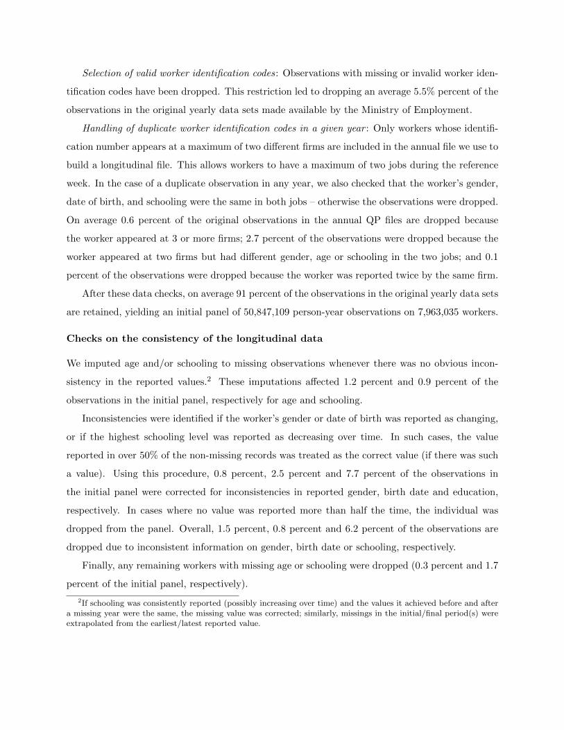
Selection of valid worker identification codes: Observations with missing or invalid worker iden-

tification codes have been dropped. This restriction led to dropping an average 5.5% percent of the

observations in the original yearly data sets made available by the Ministry of Employment.

Handling of duplicate worker identification codes in a given year : Only workers whose identifi-

cation number appears at a maximum of two different firms are included in the annual file we use to

build a longitudinal file. This allows workers to have a maximum of two jobs during the reference

week. In the case of a duplicate observation in any year, we also checked that the worker’s gender,

date of birth, and schooling were the same in both jobs – otherwise the observations were dropped.

On average 0.6 percent of the original observations in the annual QP files are dropped because

the worker appeared at 3 or more firms; 2.7 percent of the observations were dropped because the

worker appeared at two firms but had different gender, age or schooling in the two jobs; and 0.1

percent of the observations were dropped because the worker was reported twice by the same firm.

After these data checks, on average 91 percent of the observations in the original yearly data sets

are retained, yielding an initial panel of 50,847,109 person-year observations on 7,963,035 workers.

Checks on the consistency of the longitudinal data

We imputed age and/or schooling to missing observations whenever there was no obvious incon-

sistency in the reported values.2 These imputations affected 1.2 percent and 0.9 percent of the

observations in the initial panel, respectively for age and schooling.

Inconsistencies were identified if the worker’s gender or date of birth was reported as changing,

or if the highest schooling level was reported as decreasing over time. In such cases, the value

reported in over 50% of the non-missing records was treated as the correct value (if there was such

a value). Using this procedure, 0.8 percent, 2.5 percent and 7.7 percent of the observations in

the initial panel were corrected for inconsistencies in reported gender, birth date and education,

respectively. In cases where no value was reported more than half the time, the individual was

dropped from the panel. Overall, 1.5 percent, 0.8 percent and 6.2 percent of the observations are

dropped due to inconsistent information on gender, birth date or schooling, respectively.

Finally, any remaining workers with missing age or schooling were dropped (0.3 percent and 1.7

percent of the initial panel, respectively).

2If schooling was consistently reported (possibly increasing over time) and the values it achieved before and aftera missing year were the same, the missing value was corrected; similarly, missings in the initial/final period(s) wereextrapolated from the earliest/latest reported value.

The final panel data set includes 45,511,769 person-year observations for 7,159,178 workers: this

represents approximately 90 percent of the initial panel.

A final set of checks on the longitudinal data concentrated on the date of hire information.

Dates of hire later than the date of the survey reference week were considered as mistakes and

recoded to missing (affecting 3.8% of the observations). Missing information on date of hire was

imputed whenever it was consistently reported for other years in the spell (affecting 4.6% of the

observations). When the information was reported inconsistently across years, the date of hire

reported more than one-half the time was taken as the correct one, leading to corrections for 2.1%

of the observations. If after these corrections a worker had two or more dates of hire within the

same employment spell the first reported date was considered the correct date (correcting 0.9% of

the observations). Workers with inconsistent data after the introduction of the previous corrections

were assigned missing information on date of hire (0.1% of the observations).

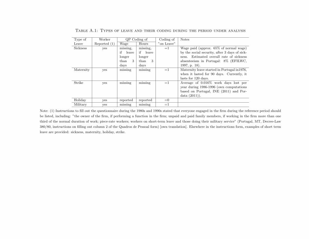
Table A.1: Types of leave and their coding during the period under analysis

Type of Worker QP Coding of Coding of NotesLeave Reported (1) Wage Hours ”on Leave”

Sickness yes missing,if leavelongerthan 3days

missing,if leavelongerthan 3days

=1 Wage paid (approx. 65% of normal wage)by the social security, after 3 days of sick-ness. Estimated overall rate of sicknessabsenteeism in Portugal: 8% (EFILWC,1997, p. 18).

Maternity yes missing missing =1 Maternity leave started in Portugal in1976,when it lasted for 90 days. Currently, itlasts for 120 days.

Strike yes missing missing =1 Average of 0.016% work days lost peryear during 1986-1996 (own computationsbased on Portugal, INE (2011) and Por-data (2011)).

Holiday yes reported reported =0

Military yes missing missing =1

Note: (1) Instructions to fill out the questionnaire during the 1980s and 1990s stated that everyone engaged in the firm during the reference period should

be listed, including: ”the owner of the firm, if performing a function in the firm; unpaid and paid family members, if working in the firm more than one

third of the normal duration of work; piece-rate workers; workers on short-term leave and those doing their military service” (Portugal, MT, Decree-Law

380/80, instructions on filling out column 2 of the Quadros de Pessoal form) [own translation]. Elsewhere in the instructions form, examples of short term

leave are provided: sickness, maternity, holiday, strike.

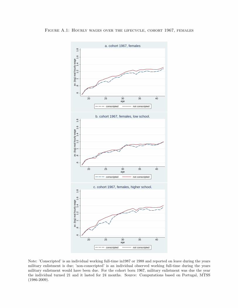
Figure A.1: Hourly wages over the lifecycle, cohort 1967, females

.6.8

11.

21.

41.

61.

8av

. (lo

g) r

eal h

ourly

wag

e

20 25 30 35 40age

conscripted not conscripted

a. cohort 1967, females

.6.8

11.

21.

41.

61.

8av

. (lo

g) r

eal h

ourly

wag

e

20 25 30 35 40age

conscripted not conscripted

b. cohort 1967, females, low school.

.6.8

11.

21.

41.

61.

8av

. (lo

g) r

eal h

ourly

wag

e

20 25 30 35 40age

conscripted not conscripted

c. cohort 1967, females, higher school.

Note: ’Conscripted’ is an individual working full-time in1987 or 1988 and reported on leave during the yearsmilitary enlistment is due; ’non-conscripted’ is an individual observed working full-time during the yearsmilitary enlistment would have been due. For the cohort born 1967, military enlistment was due the yearthe individual turned 21 and it lasted for 24 months. Source: Computations based on Portugal, MTSS(1986-2009).

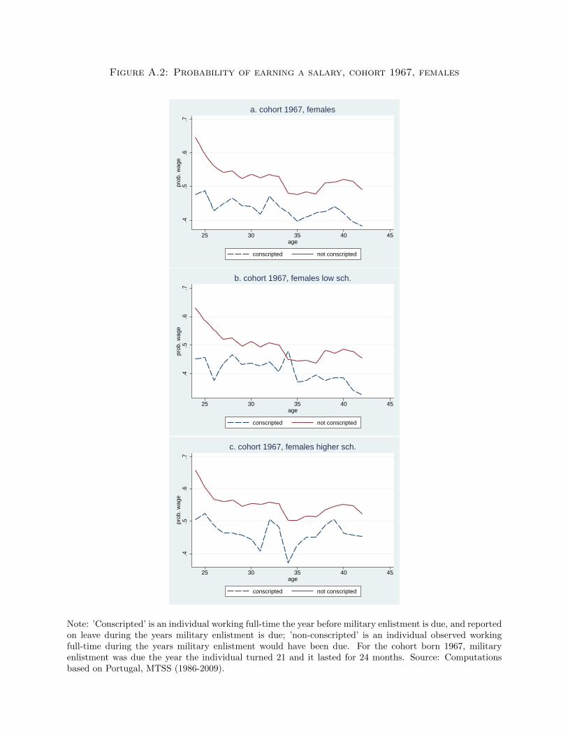
Figure A.2: Probability of earning a salary, cohort 1967, females

.4.5

.6.7

prob

. wag

e

25 30 35 40 45age

conscripted not conscripted

a. cohort 1967, females

.4.5

.6.7

prob

. wag

e

25 30 35 40 45age

conscripted not conscripted

b. cohort 1967, females low sch.

.4.5

.6.7

prob

. wag

e

25 30 35 40 45age

conscripted not conscripted

c. cohort 1967, females higher sch.

Note: ’Conscripted’ is an individual working full-time the year before military enlistment is due, and reportedon leave during the years military enlistment is due; ’non-conscripted’ is an individual observed workingfull-time during the years military enlistment would have been due. For the cohort born 1967, militaryenlistment was due the year the individual turned 21 and it lasted for 24 months. Source: Computationsbased on Portugal, MTSS (1986-2009).

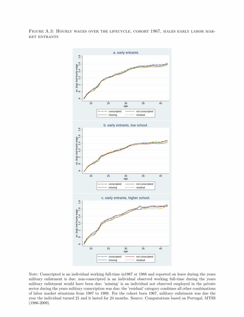
Figure A.3: Hourly wages over the lifecycle, cohort 1967, males early labor mar-ket entrants

.6.8

11.

21.

41.

61.

8av

. (lo

g) r

eal h

ourly

wag

e

20 25 30 35 40age

conscripted not conscriptedmissing residual

a. early entrants

.6.8

11.

21.

41.

61.

8av

. (lo

g) r

eal h

ourly

wag

e

20 25 30 35 40age

conscripted not conscriptedmissing residual

b. early entrants, low school.

.6.8

11.

21.

41.

61.

8av

. (lo

g) r

eal h

ourly

wag

e

20 25 30 35 40age

conscripted not conscriptedmissing residual

c. early entrants, higher school.

Note: Conscripted is an individual working full-time in1987 or 1988 and reported on leave during the yearsmilitary enlistment is due; non-conscripted is an individual observed working full-time during the yearsmilitary enlistment would have been due; ’missing’ is an individual not observed employed in the privatesector during the years military conscription was due; the ’residual’ category combines all other combinationsof labor market situations from 1987 to 1989. For the cohort born 1967, military enlistment was due theyear the individual turned 21 and it lasted for 24 months. Source: Computations based on Portugal, MTSS(1986-2009).

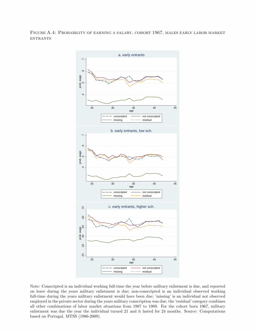
Figure A.4: Probability of earning a salary, cohort 1967, males early labor marketentrants

.4.5

.6.7

prob

. wag

e

25 30 35 40 45age

conscripted not conscriptedmissing residual

a. early entrants

.4.5

.6.7

prob

. wag

e

25 30 35 40 45age

conscripted not conscriptedmissing residual

b. early entrants, low sch.

.23

.33

.43

.53

.63

.73

prob

. wag

e

25 30 35 40 45age

conscripted not conscriptedmissing residual

c. early entrants, higher sch.

Note: Conscripted is an individual working full-time the year before military enlistment is due, and reportedon leave during the years military enlistment is due; non-conscripted is an individual observed workingfull-time during the years military enlistment would have been due; ’missing’ is an individual not observedemployed in the private sector during the years military conscription was due; the ’residual’ category combinesall other combinations of labor market situations from 1987 to 1989. For the cohort born 1967, militaryenlistment was due the year the individual turned 21 and it lasted for 24 months. Source: Computationsbased on Portugal, MTSS (1986-2009).

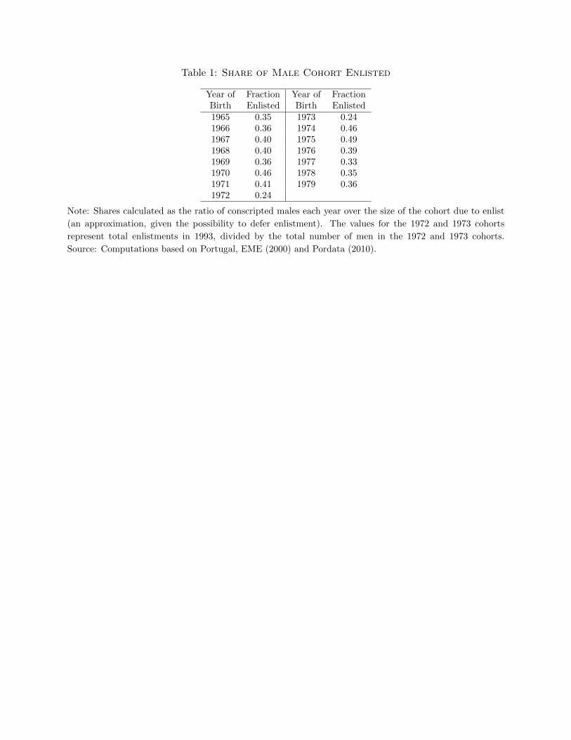
Table 1: Share of Male Cohort Enlisted

Year of Fraction Year of FractionBirth Enlisted Birth Enlisted1965 0.35 1973 0.241966 0.36 1974 0.461967 0.40 1975 0.491968 0.40 1976 0.391969 0.36 1977 0.331970 0.46 1978 0.351971 0.41 1979 0.361972 0.24

Note: Shares calculated as the ratio of conscripted males each year over the size of the cohort due to enlist

(an approximation, given the possibility to defer enlistment). The values for the 1972 and 1973 cohorts

represent total enlistments in 1993, divided by the total number of men in the 1972 and 1973 cohorts.

Source: Computations based on Portugal, EME (2000) and Pordata (2010).

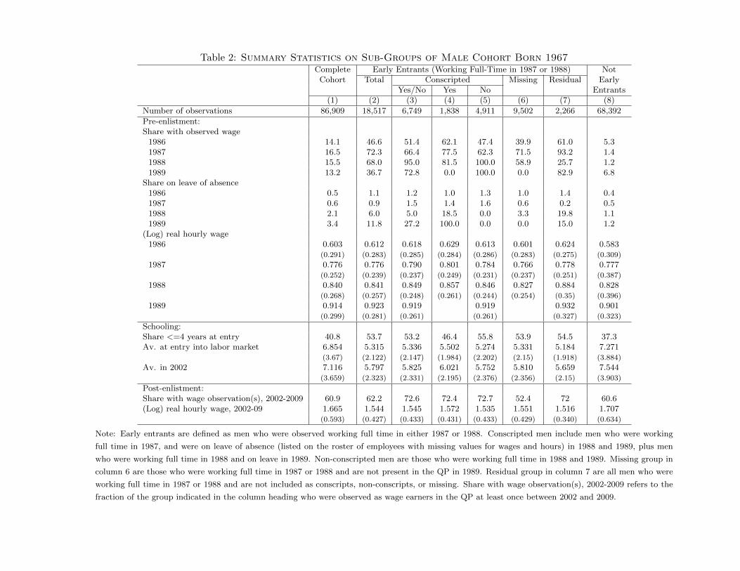
Table 2: Summary Statistics on Sub-Groups of Male Cohort Born 1967Complete Early Entrants (Working Full-Time in 1987 or 1988) NotCohort Total Conscripted Missing Residual Early

Yes/No Yes No Entrants(1) (2) (3) (4) (5) (6) (7) (8)

Number of observations 86,909 18,517 6,749 1,838 4,911 9,502 2,266 68,392

Pre-enlistment:Share with observed wage

1986 14.1 46.6 51.4 62.1 47.4 39.9 61.0 5.31987 16.5 72.3 66.4 77.5 62.3 71.5 93.2 1.41988 15.5 68.0 95.0 81.5 100.0 58.9 25.7 1.21989 13.2 36.7 72.8 0.0 100.0 0.0 82.9 6.8

Share on leave of absence1986 0.5 1.1 1.2 1.0 1.3 1.0 1.4 0.41987 0.6 0.9 1.5 1.4 1.6 0.6 0.2 0.51988 2.1 6.0 5.0 18.5 0.0 3.3 19.8 1.11989 3.4 11.8 27.2 100.0 0.0 0.0 15.0 1.2

(Log) real hourly wage1986 0.603 0.612 0.618 0.629 0.613 0.601 0.624 0.583

(0.291) (0.283) (0.285) (0.284) (0.286) (0.283) (0.275) (0.309)

1987 0.776 0.776 0.790 0.801 0.784 0.766 0.778 0.777(0.252) (0.239) (0.237) (0.249) (0.231) (0.237) (0.251) (0.387)

1988 0.840 0.841 0.849 0.857 0.846 0.827 0.884 0.828(0.268) (0.257) (0.248) (0.261) (0.244) (0.254) (0.35) (0.396)

1989 0.914 0.923 0.919 0.919 0.932 0.901(0.299) (0.281) (0.261) (0.261) (0.327) (0.323)

Schooling:Share <=4 years at entry 40.8 53.7 53.2 46.4 55.8 53.9 54.5 37.3Av. at entry into labor market 6.854 5.315 5.336 5.502 5.274 5.331 5.184 7.271

(3.67) (2.122) (2.147) (1.984) (2.202) (2.15) (1.918) (3.884)

Av. in 2002 7.116 5.797 5.825 6.021 5.752 5.810 5.659 7.544(3.659) (2.323) (2.331) (2.195) (2.376) (2.356) (2.15) (3.903)

Post-enlistment:Share with wage observation(s), 2002-2009 60.9 62.2 72.6 72.4 72.7 52.4 72 60.6(Log) real hourly wage, 2002-09 1.665 1.544 1.545 1.572 1.535 1.551 1.516 1.707

(0.593) (0.427) (0.433) (0.431) (0.433) (0.429) (0.340) (0.634)

Note: Early entrants are defined as men who were observed working full time in either 1987 or 1988. Conscripted men include men who were working

full time in 1987, and were on leave of absence (listed on the roster of employees with missing values for wages and hours) in 1988 and 1989, plus men

who were working full time in 1988 and on leave in 1989. Non-conscripted men are those who were working full time in 1988 and 1989. Missing group in

column 6 are those who were working full time in 1987 or 1988 and are not present in the QP in 1989. Residual group in column 7 are all men who were

working full time in 1987 or 1988 and are not included as conscripts, non-conscripts, or missing. Share with wage observation(s), 2002-2009 refers to the

fraction of the group indicated in the column heading who were observed as wage earners in the QP at least once between 2002 and 2009.

Table 3a: Estimated Wage Effects of Conscription at Various Ages from Alternative Models (Pooled Edu-cation Groups)

OLS Model with No OLS Model Including Differenced Model: Quasi-Differenced Model:Control for Wage at Control for Wage at Wage Minus Wage at Wage Minus 4.16 x Wage at

Age 20/21 Age 20/21 Age 20/21 Age 20/21Age Conscription Std. Conscription Std. Conscription Std. Conscription Std.

Effect Error Effect Error Effect Error Effect Error(1) (2) (3) (4) (5) (6) (7) (8)

19 1.0 (1.0)20 1.0 (0.8)21 0.2 (0.7)

24 -1.4 (1.1) -1.8 (1.0) -2.1 (1.1) -4.2 (3.2)25 1.7 (1.2) 1.4 (1.1) 1.0 (1.2) -1.0 (3.4)26 1.5 (1.3) 1.4 (1.2) 1.3 (1.3) 0.9 (3.5)27 1.2 (1.4) 1.1 (1.3) 0.9 (1.4) 0.0 (3.7)28 1.8 (1.3) 1.5 (1.2) 1.1 (1.3) -1.2 (3.6)29 2.6 (1.4) 2.2 (1.4) 1.7 (1.5) -1.1 (3.7)30 0.6 (1.3) 0.6 (1.3) 0.6 (1.4) 0.6 (3.6)31 1.4 (1.3) 1.0 (1.2) 0.5 (1.4) -2.0 (3.6)32 0.9 (1.3) 0.6 (1.2) 0.1 (1.3) -2.2 (3.6)33 1.2 (1.3) 1.2 (1.3) 1.0 (1.4) 0.4 (3.5)

35 0.8 (1.4) 0.9 (1.4) 0.9 (1.5) 1.1 (3.6)36 2.2 (1.4) 2.3 (1.4) 2.4 (1.5) 3.2 (3.8)37 0.4 (1.4) 0.6 (1.4) 0.9 (1.5) 2.4 (3.8)38 2.2 (1.4) 2.1 (1.4) 2.0 (1.5) 1.3 (3.6)39 3.0 (1.5) 2.8 (1.4) 2.6 (1.5) 1.1 (3.7)40 3.7 (1.5) 3.5 (1.4) 3.1 (1.5) 1.3 (3.6)41 2.5 (1.4) 2.4 (1.4) 2.2 (1.5) 1.4 (3.7)42 1.7 (1.5) 1.8 (1.5) 2.1 (1.6) 3.3 (3.7)

Pooled: 24-33 1.1 (0.9) 0.9 (0.8) 0.6 (0.9) -1.0 (3.2)Pooled: 35-42 2.1 (1.2) 2.1 (1.2) 2.0 (1.3) 1.9 (3.5)

Notes: Estimated coefficients times 100 (with standard errors in parentheses) from models fit separately by age to wages of conscripts and non-conscripts.

All models include dummies for education as of age 20 or 21. Models in columns 3-4 include wage measured at age 20 or 21. Models in columns 5-6 use

as dependent variable wage at indicated age, minus wage at age 20/21. Models in columns 7-8 use as dependent variable wage at indicated age minus

4.16 times wage at age 20/21. Pooled estimates use sample of available person-year observations, and include year dummies. Standard errors for pooled

models are clustered by person. Source: Portugal, MTSS (1986-2009).

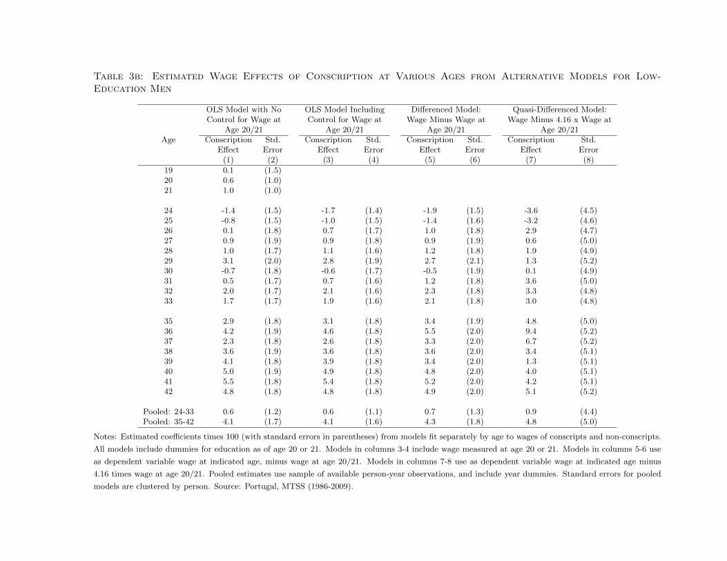
Table 3b: Estimated Wage Effects of Conscription at Various Ages from Alternative Models for Low-Education Men

OLS Model with No OLS Model Including Differenced Model: Quasi-Differenced Model:Control for Wage at Control for Wage at Wage Minus Wage at Wage Minus 4.16 x Wage at

Age 20/21 Age 20/21 Age 20/21 Age 20/21Age Conscription Std. Conscription Std. Conscription Std. Conscription Std.

Effect Error Effect Error Effect Error Effect Error(1) (2) (3) (4) (5) (6) (7) (8)

19 0.1 (1.5)20 0.6 (1.0)21 1.0 (1.0)

24 -1.4 (1.5) -1.7 (1.4) -1.9 (1.5) -3.6 (4.5)25 -0.8 (1.5) -1.0 (1.5) -1.4 (1.6) -3.2 (4.6)26 0.1 (1.8) 0.7 (1.7) 1.0 (1.8) 2.9 (4.7)27 0.9 (1.9) 0.9 (1.8) 0.9 (1.9) 0.6 (5.0)28 1.0 (1.7) 1.1 (1.6) 1.2 (1.8) 1.9 (4.9)29 3.1 (2.0) 2.8 (1.9) 2.7 (2.1) 1.3 (5.2)30 -0.7 (1.8) -0.6 (1.7) -0.5 (1.9) 0.1 (4.9)31 0.5 (1.7) 0.7 (1.6) 1.2 (1.8) 3.6 (5.0)32 2.0 (1.7) 2.1 (1.6) 2.3 (1.8) 3.3 (4.8)33 1.7 (1.7) 1.9 (1.6) 2.1 (1.8) 3.0 (4.8)

35 2.9 (1.8) 3.1 (1.8) 3.4 (1.9) 4.8 (5.0)36 4.2 (1.9) 4.6 (1.8) 5.5 (2.0) 9.4 (5.2)37 2.3 (1.8) 2.6 (1.8) 3.3 (2.0) 6.7 (5.2)38 3.6 (1.9) 3.6 (1.8) 3.6 (2.0) 3.4 (5.1)39 4.1 (1.8) 3.9 (1.8) 3.4 (2.0) 1.3 (5.1)40 5.0 (1.9) 4.9 (1.8) 4.8 (2.0) 4.0 (5.1)41 5.5 (1.8) 5.4 (1.8) 5.2 (2.0) 4.2 (5.1)42 4.8 (1.8) 4.8 (1.8) 4.9 (2.0) 5.1 (5.2)

Pooled: 24-33 0.6 (1.2) 0.6 (1.1) 0.7 (1.3) 0.9 (4.4)Pooled: 35-42 4.1 (1.7) 4.1 (1.6) 4.3 (1.8) 4.8 (5.0)

Notes: Estimated coefficients times 100 (with standard errors in parentheses) from models fit separately by age to wages of conscripts and non-conscripts.

All models include dummies for education as of age 20 or 21. Models in columns 3-4 include wage measured at age 20 or 21. Models in columns 5-6 use

as dependent variable wage at indicated age, minus wage at age 20/21. Models in columns 7-8 use as dependent variable wage at indicated age minus

4.16 times wage at age 20/21. Pooled estimates use sample of available person-year observations, and include year dummies. Standard errors for pooled

models are clustered by person. Source: Portugal, MTSS (1986-2009).

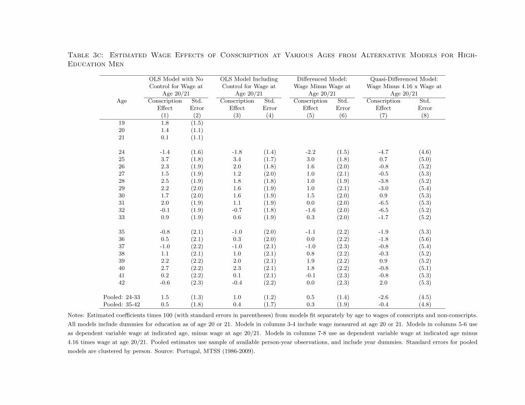
Table 3c: Estimated Wage Effects of Conscription at Various Ages from Alternative Models for High-Education Men

OLS Model with No OLS Model Including Differenced Model: Quasi-Differenced Model:Control for Wage at Control for Wage at Wage Minus Wage at Wage Minus 4.16 x Wage at

Age 20/21 Age 20/21 Age 20/21 Age 20/21Age Conscription Std. Conscription Std. Conscription Std. Conscription Std.

Effect Error Effect Error Effect Error Effect Error(1) (2) (3) (4) (5) (6) (7) (8)

19 1.8 (1.5)20 1.4 (1.1)21 0.1 (1.1)

24 -1.4 (1.6) -1.8 (1.4) -2.2 (1.5) -4.7 (4.6)25 3.7 (1.8) 3.4 (1.7) 3.0 (1.8) 0.7 (5.0)26 2.3 (1.9) 2.0 (1.8) 1.6 (2.0) -0.8 (5.2)27 1.5 (1.9) 1.2 (2.0) 1.0 (2.1) -0.5 (5.3)28 2.5 (1.9) 1.8 (1.8) 1.0 (1.9) -3.8 (5.2)29 2.2 (2.0) 1.6 (1.9) 1.0 (2.1) -3.0 (5.4)30 1.7 (2.0) 1.6 (1.9) 1.5 (2.0) 0.9 (5.3)31 2.0 (1.9) 1.1 (1.9) 0.0 (2.0) -6.5 (5.3)32 -0.1 (1.9) -0.7 (1.8) -1.6 (2.0) -6.5 (5.2)33 0.9 (1.9) 0.6 (1.9) 0.3 (2.0) -1.7 (5.2)

35 -0.8 (2.1) -1.0 (2.0) -1.1 (2.2) -1.9 (5.3)36 0.5 (2.1) 0.3 (2.0) 0.0 (2.2) -1.8 (5.6)37 -1.0 (2.2) -1.0 (2.1) -1.0 (2.3) -0.8 (5.4)38 1.1 (2.1) 1.0 (2.1) 0.8 (2.2) -0.3 (5.2)39 2.2 (2.2) 2.0 (2.1) 1.9 (2.2) 0.9 (5.2)40 2.7 (2.2) 2.3 (2.1) 1.8 (2.2) -0.8 (5.1)41 0.2 (2.2) 0.1 (2.1) -0.1 (2.3) -0.8 (5.3)42 -0.6 (2.3) -0.4 (2.2) 0.0 (2.3) 2.0 (5.3)

Pooled: 24-33 1.5 (1.3) 1.0 (1.2) 0.5 (1.4) -2.6 (4.5)Pooled: 35-42 0.5 (1.8) 0.4 (1.7) 0.3 (1.9) -0.4 (4.8)

Notes: Estimated coefficients times 100 (with standard errors in parentheses) from models fit separately by age to wages of conscripts and non-conscripts.

All models include dummies for education as of age 20 or 21. Models in columns 3-4 include wage measured at age 20 or 21. Models in columns 5-6 use

as dependent variable wage at indicated age, minus wage at age 20/21. Models in columns 7-8 use as dependent variable wage at indicated age minus

4.16 times wage at age 20/21. Pooled estimates use sample of available person-year observations, and include year dummies. Standard errors for pooled

models are clustered by person. Source: Portugal, MTSS (1986-2009).

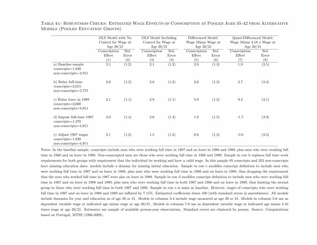
Table 4a: Robustness Checks: Estimated Wage Effects of Conscription at Pooled Ages 35-42 from AlternativeModels (Pooled Education Groups)

OLS Model with No OLS Model Including Differenced Model: Quasi-Differenced Model:Control for Wage at Control for Wage at Wage Minus Wage at Wage Minus 4.16 x Wage at

Age 20/21 Age 20/21 Age 20/21 Age 20/21Conscription Std. Conscription Std. Conscription Std. Conscription Std.

Effect Error Effect Error Effect Error Effect Error(1) (2) (3) (4) (5) (6) (7) (8)

a) Baseline sample 2.1 (1.2) 2.1 (1.2) 2.0 (1.3) 1.9 (3.5)conscripts=1,838non-conscripts=4,911

b) Relax full-time 2.6 (1.2) 2.6 (1.2) 2.6 (1.3) 2.7 (3.4)conscripts=2,015non-conscripts=5,775

c) Relax leave in 1989 2.1 (1.1) 2.8 (1.1) 3.8 (1.2) 9.2 (3.1)conscripts=2,600non-conscripts=4,911

d) Impose full-time 1987 3.0 (1.4) 2.6 (1.3) 1.9 (1.5) -1.7 (3.9)conscripts=1,370non-conscripts=4,911

e) Adjust 1987 wages 2.1 (1.2) 1.5 (1.2) 0.6 (1.3) -3.9 (3.5)conscripts=1,838non-conscripts=4,911

Notes: In the baseline sample, conscripts include men who were working full time in 1987 and on leave in 1988 and 1989, plus men who were working full

time in 1988 and on leave in 1989. Non-conscripted men are those who were working full time in 1988 and 1989. Sample in row b replaces full time work

requirements for both groups with requirement that the individual be working and have a valid wage. In this sample 95 conscripts and 352 non-conscripts

have missing education data: models include a dummy for missing initial education. Sample in row c modifies conscript definition to include men who

were working full time in 1987 and on leave in 1988, plus men who were working full time in 1988 and on leave in 1989, thus dropping the requirement

that the men who worked full time in 1987 were also on leave in 1989. Sample in row d modifies conscript definition to include men who were working full

time in 1987 and on leave in 1988 and 1989, plus men who were working full time in both 1987 and 1988 and on leave in 1989, thus limiting the second

group to those who were working full time in both 1987 and 1988. Sample in row e is same as baseline. However, wages of conscripts who were working

full time in 1987 and on leave in 1988 and 1989 are inflated by 7.15%. Estimated coefficients times 100 (with standard errors in parentheses). All models

include dummies for year and education as of age 20 or 21. Models in columns 3-4 include wage measured at age 20 or 21. Models in columns 5-6 use as

dependent variable wage at indicated age minus wage at age 20/21. Models in columns 7-8 use as dependent variable wage at indicated age minus 4.16

times wage at age 20/21. Estimates use sample of available person-year observations. Standard errors are clustered by person. Source: Computations

based on Portugal, MTSS (1986-2009).

Table 4b: Robustness Checks: Estimated Wage Effects of Conscription at Pooled Ages 35-42 from AlternativeModels (Low-Education Men)

OLS Model with No OLS Model Including Differenced Model: Quasi-Differenced Model:Control for Wage at Control for Wage at Wage Minus Wage at Wage Minus 4.16 x Wage at

Age 20/21 Age 20/21 Age 20/21 Age 20/21Conscription Std. Conscription Std. Conscription Std. Conscription Std.

Effect Error Effect Error Effect Error Effect Error(1) (2) (3) (4) (5) (6) (7) (8)

a) Baseline sample 4.1 (1.7) 4.1 (1.6) 4.3 (1.8) 4.8 (5.0)conscripts=821non-conscripts=2,675

b) Relax full-time 4.7 (1.6) 4.7 (1.5) 4.7 (1.7) 4.6 (4.9)conscripts=850non-conscripts=2,999

c) Relax leave in 1989 3.8 (1.4) 4.6 (1.4) 6.2 (1.5) 13.6 (4.3)conscripts=1,187non-conscripts=2,675

d) Impose full-time 1987 5.4 (1.9) 5.1 (1.9) 4.5 (2.1) 1.7 (5.7)conscripts=608non-conscripts=2,675

e) Adjust 1987 wages 4.1 (1.7) 3.7 (1.6) 2.8 (1.7) -1.3 (5.0)conscripts=821non-conscripts=2,675

Notes: In the baseline sample, conscripts include men who were working full time in 1987 and on leave in 1988 and 1989, plus men who were working full

time in 1988 and on leave in 1989. Non-conscripted men are those who were working full time in 1988 and 1989. Sample in row b replaces full time work

requirements for both groups with requirement that the individual be working and have a valid wage. In this sample 95 conscripts and 352 non-conscripts

have missing education data: models include a dummy for missing initial education. Sample in row c modifies conscript definition to include men who

were working full time in 1987 and on leave in 1988, plus men who were working full time in 1988 and on leave in 1989, thus dropping the requirement

that the men who worked full time in 1987 were also on leave in 1989. Sample in row d modifies conscript definition to include men who were working full

time in 1987 and on leave in 1988 and 1989, plus men who were working full time in both 1987 and 1988 and on leave in 1989, thus limiting the second

group to those who were working full time in both 1987 and 1988. Sample in row e is same as baseline. However, wages of conscripts who were working

full time in 1987 and on leave in 1988 and 1989 are inflated by 7.15%. Estimated coefficients times 100 (with standard errors in parentheses). All models

include dummies for year and education as of age 20 or 21. Models in columns 3-4 include wage measured at age 20 or 21. Models in columns 5-6 use as

dependent variable wage at indicated age minus wage at age 20/21. Models in columns 7-8 use as dependent variable wage at indicated age minus 4.16

times wage at age 20/21. Estimates use sample of available person-year observations. Standard errors are clustered by person. Source: Computations

based on Portugal, MTSS (1986-2009).

Table 4c: Robustness Checks: Estimated Wage Effects of Conscription at Pooled Ages 35-42 from AlternativeModels (High-Education Men)

OLS Model with No OLS Model Including Differenced Model: Quasi-Differenced Model:Control for Wage at Control for Wage at Wage Minus Wage at Wage Minus 4.16 x Wage at

Age 20/21 Age 20/21 Age 20/21 Age 20/21Conscription Std. Conscription Std. Conscription Std. Conscription Std.

Effect Error Effect Error Effect Error Effect Error(1) (2) (3) (4) (5) (6) (7) (8)

a) Baseline sample 0.5 (1.8) 0.4 (1.7) 0.3 (1.9) -0.4 (4.8)conscripts=1,017non-conscripts=2,236

b) Relax full-time 0.6 (1.7) 1.0 (1.7) 1.0 (1.8) 1.2 (4.6)conscripts=1,070non-conscripts=2,424

c) Relax leave in 1989 0.7 (1.6) 1.2 (1.6) 1.9 (1.7) 5.5 (4.3)conscripts=1,413non-conscripts=2,236

d) Impose full-time 1987 1.2 (1.9) 0.6 (1.9) -0.1 (2.0) -4.2 (5.2)conscripts=762non-conscripts=2,236

e) Adjust 1987 wages 0.5 (1.8) -0.1 (1.7) -1.0 (1.9) -5.9 (4.8)conscripts=1,017non-conscripts=2,236

Notes: In the baseline sample, conscripts include men who were working full time in 1987 and on leave in 1988 and 1989, plus men who were working full

time in 1988 and on leave in 1989. Non-conscripted men are those who were working full time in 1988 and 1989. Sample in row b replaces full time work

requirements for both groups with requirement that the individual be working and have a valid wage. In this sample 95 conscripts and 352 non-conscripts

have missing education data: models include a dummy for missing initial education. Sample in row c modifies conscript definition to include men who

were working full time in 1987 and on leave in 1988, plus men who were working full time in 1988 and on leave in 1989, thus dropping the requirement

that the men who worked full time in 1987 were also on leave in 1989. Sample in row d modifies conscript definition to include men who were working full

time in 1987 and on leave in 1988 and 1989, plus men who were working full time in both 1987 and 1988 and on leave in 1989, thus limiting the second

group to those who were working full time in both 1987 and 1988. Sample in row e is same as baseline. However, wages of conscripts who were working

full time in 1987 and on leave in 1988 and 1989 are inflated by 7.15%. Estimated coefficients times 100 (with standard errors in parentheses). All models

include dummies for year and education as of age 20 or 21. Models in columns 3-4 include wage measured at age 20 or 21. Models in columns 5-6 use as

dependent variable wage at indicated age minus wage at age 20/21. Models in columns 7-8 use as dependent variable wage at indicated age minus 4.16

times wage at age 20/21. Estimates use sample of available person-year observations. Standard errors are clustered by person. Source: Computations

based on Portugal, MTSS (1986-2009).

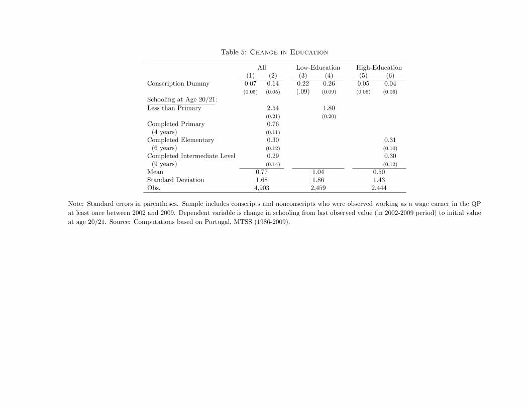
Table 5: Change in Education

All Low-Education High-Education(1) (2) (3) (4) (5) (6)

Conscription Dummy 0.07 0.14 0.22 0.26 0.05 0.04(0.05) (0.05) (.09) (0.09) (0.06) (0.06)

Schooling at Age 20/21:

Less than Primary 2.54 1.80(0.21) (0.20)

Completed Primary 0.76(4 years) (0.11)

Completed Elementary 0.30 0.31(6 years) (0.12) (0.10)

Completed Intermediate Level 0.29 0.30(9 years) (0.14) (0.12)

Mean 0.77 1.04 0.50Standard Deviation 1.68 1.86 1.43Obs. 4,903 2,459 2,444

Note: Standard errors in parentheses. Sample includes conscripts and nonconscripts who were observed working as a wage earner in the QP

at least once between 2002 and 2009. Dependent variable is change in schooling from last observed value (in 2002-2009 period) to initial value

at age 20/21. Source: Computations based on Portugal, MTSS (1986-2009).

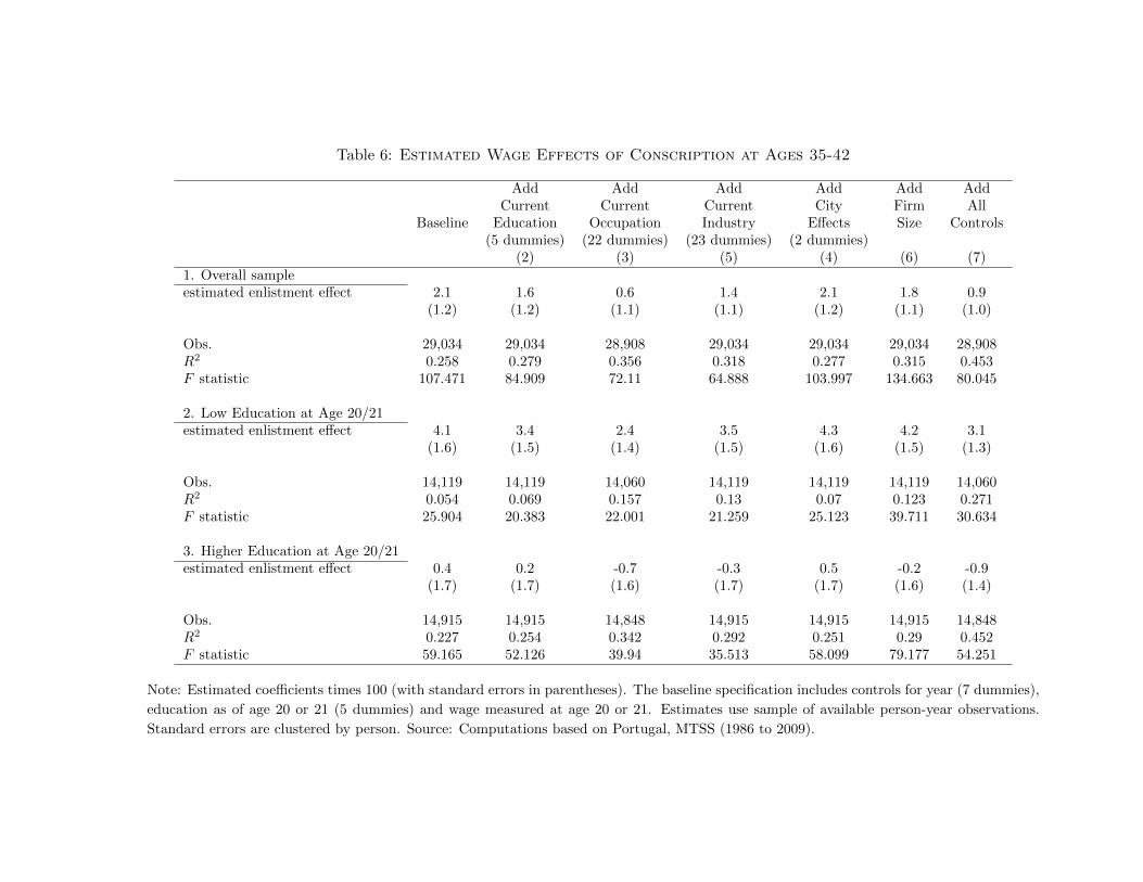
Table 6: Estimated Wage Effects of Conscription at Ages 35-42

Add Add Add Add Add AddCurrent Current Current City Firm All

Baseline Education Occupation Industry Effects Size Controls(5 dummies) (22 dummies) (23 dummies) (2 dummies)

(2) (3) (5) (4) (6) (7)1. Overall sampleestimated enlistment effect 2.1 1.6 0.6 1.4 2.1 1.8 0.9

(1.2) (1.2) (1.1) (1.1) (1.2) (1.1) (1.0)

Obs. 29,034 29,034 28,908 29,034 29,034 29,034 28,908R2 0.258 0.279 0.356 0.318 0.277 0.315 0.453F statistic 107.471 84.909 72.11 64.888 103.997 134.663 80.045

2. Low Education at Age 20/21estimated enlistment effect 4.1 3.4 2.4 3.5 4.3 4.2 3.1

(1.6) (1.5) (1.4) (1.5) (1.6) (1.5) (1.3)

Obs. 14,119 14,119 14,060 14,119 14,119 14,119 14,060R2 0.054 0.069 0.157 0.13 0.07 0.123 0.271F statistic 25.904 20.383 22.001 21.259 25.123 39.711 30.634

3. Higher Education at Age 20/21estimated enlistment effect 0.4 0.2 -0.7 -0.3 0.5 -0.2 -0.9

(1.7) (1.7) (1.6) (1.7) (1.7) (1.6) (1.4)

Obs. 14,915 14,915 14,848 14,915 14,915 14,915 14,848R2 0.227 0.254 0.342 0.292 0.251 0.29 0.452F statistic 59.165 52.126 39.94 35.513 58.099 79.177 54.251

Note: Estimated coefficients times 100 (with standard errors in parentheses). The baseline specification includes controls for year (7 dummies),

education as of age 20 or 21 (5 dummies) and wage measured at age 20 or 21. Estimates use sample of available person-year observations.

Standard errors are clustered by person. Source: Computations based on Portugal, MTSS (1986 to 2009).

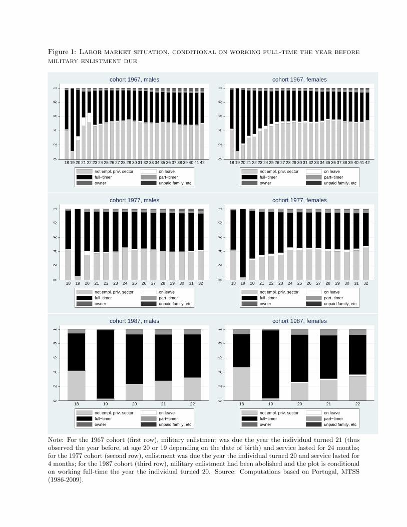
Figure 1: Labor market situation, conditional on working full-time the year beforemilitary enlistment due

0.2

.4.6

.81

18 19 20 21 22 23 24 25 26 27 28 29 30 31 32 33 34 35 36 37 38 39 40 41 42

cohort 1967, males

not empl. priv. sector on leavefull−timer part−timerowner unpaid family, etc

0.2

.4.6

.81

18 19 20 21 22 23 24 25 26 27 28 29 30 31 32 33 34 35 36 37 38 39 40 41 42

cohort 1967, females

not empl. priv. sector on leavefull−timer part−timerowner unpaid family, etc

0.2

.4.6

.81

18 19 20 21 22 23 24 25 26 27 28 29 30 31 32

cohort 1977, males

not empl. priv. sector on leavefull−timer part−timerowner unpaid family, etc

0.2

.4.6

.81

18 19 20 21 22 23 24 25 26 27 28 29 30 31 32

cohort 1977, females

not empl. priv. sector on leavefull−timer part−timerowner unpaid family, etc

0.2

.4.6

.81

18 19 20 21 22

cohort 1987, males

not empl. priv. sector on leavefull−timer part−timerowner unpaid family, etc

0.2

.4.6

.81

18 19 20 21 22

cohort 1987, females

not empl. priv. sector on leavefull−timer part−timerowner unpaid family, etc

Note: For the 1967 cohort (first row), military enlistment was due the year the individual turned 21 (thusobserved the year before, at age 20 or 19 depending on the date of birth) and service lasted for 24 months;for the 1977 cohort (second row), enlistment was due the year the individual turned 20 and service lasted for4 months; for the 1987 cohort (third row), military enlistment had been abolished and the plot is conditionalon working full-time the year the individual turned 20. Source: Computations based on Portugal, MTSS(1986-2009).

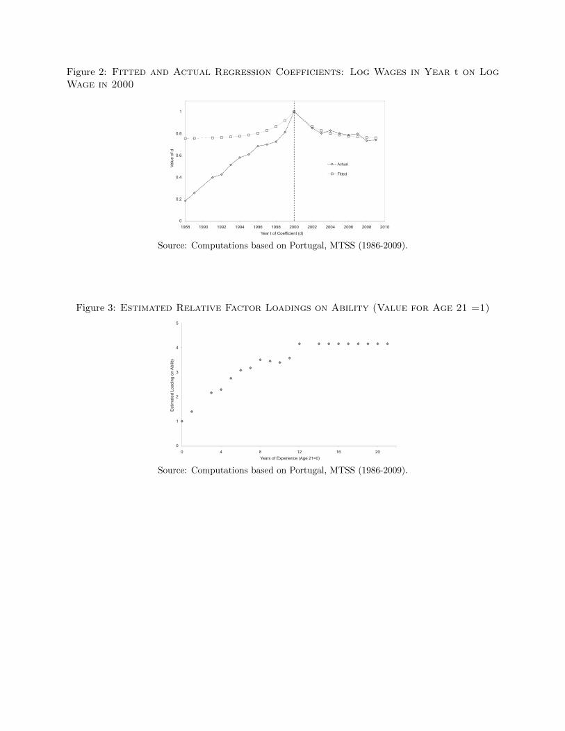
Figure 2: Fitted and Actual Regression Coefficients: Log Wages in Year t on LogWage in 2000

0.8

1

f d

0

0.2

0.4

0.6

1988 1990 1992 1994 1996 1998 2000 2002 2004 2006 2008 2010

Va

lue

of

Year t of Coefficient (d)

Actual

Fitted

Source: Computations based on Portugal, MTSS (1986-2009).

Figure 3: Estimated Relative Factor Loadings on Ability (Value for Age 21 =1)

3

4

5

on A

bili

ty

0

1

2

0 4 8 12 16 20

Estim

ate

d L

oa

din

g o

Years of Experience (Age 21=0)

Source: Computations based on Portugal, MTSS (1986-2009).

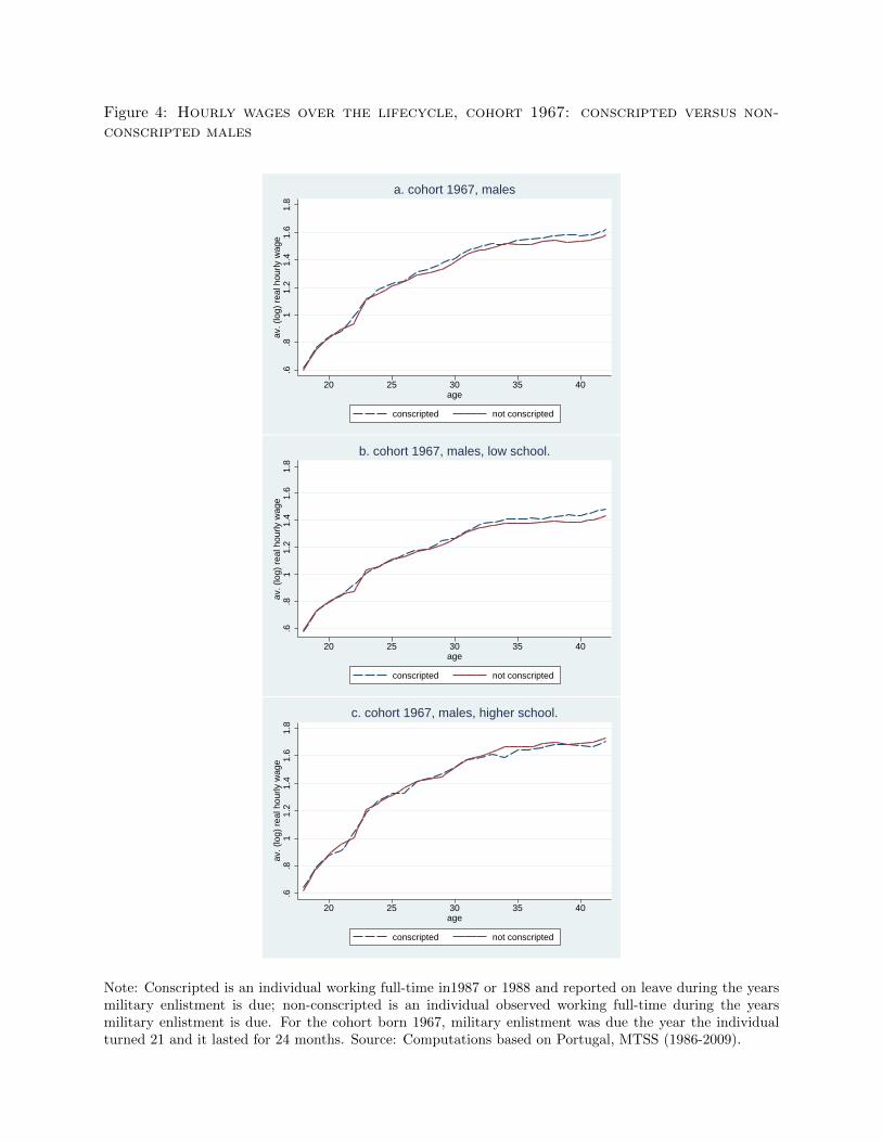
Figure 4: Hourly wages over the lifecycle, cohort 1967: conscripted versus non-conscripted males

.6.8

11.

21.

41.

61.

8av

. (lo

g) r

eal h

ourly

wag

e

20 25 30 35 40age

conscripted not conscripted

a. cohort 1967, males

.6.8

11.

21.

41.

61.

8av

. (lo

g) r

eal h

ourly

wag

e

20 25 30 35 40age

conscripted not conscripted

b. cohort 1967, males, low school.

.6.8

11.

21.

41.

61.

8av

. (lo

g) r

eal h

ourly

wag

e

20 25 30 35 40age

conscripted not conscripted

c. cohort 1967, males, higher school.

Note: Conscripted is an individual working full-time in1987 or 1988 and reported on leave during the yearsmilitary enlistment is due; non-conscripted is an individual observed working full-time during the yearsmilitary enlistment is due. For the cohort born 1967, military enlistment was due the year the individualturned 21 and it lasted for 24 months. Source: Computations based on Portugal, MTSS (1986-2009).

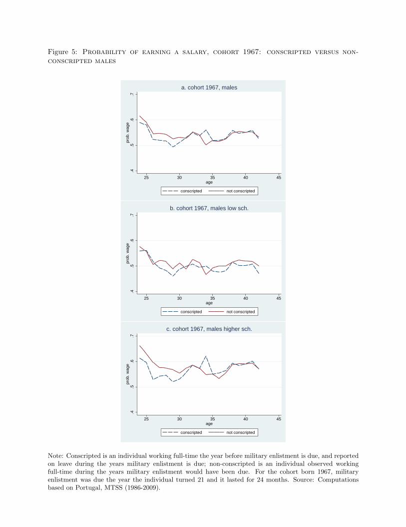
Figure 5: Probability of earning a salary, cohort 1967: conscripted versus non-conscripted males

.4.5

.6.7

prob

. wag

e

25 30 35 40 45age

conscripted not conscripted

a. cohort 1967, males

.4.5

.6.7

prob

. wag

e

25 30 35 40 45age

conscripted not conscripted

b. cohort 1967, males low sch.

.4.5

.6.7

prob

. wag

e

25 30 35 40 45age

conscripted not conscripted

c. cohort 1967, males higher sch.

Note: Conscripted is an individual working full-time the year before military enlistment is due, and reportedon leave during the years military enlistment is due; non-conscripted is an individual observed workingfull-time during the years military enlistment would have been due. For the cohort born 1967, militaryenlistment was due the year the individual turned 21 and it lasted for 24 months. Source: Computationsbased on Portugal, MTSS (1986-2009).

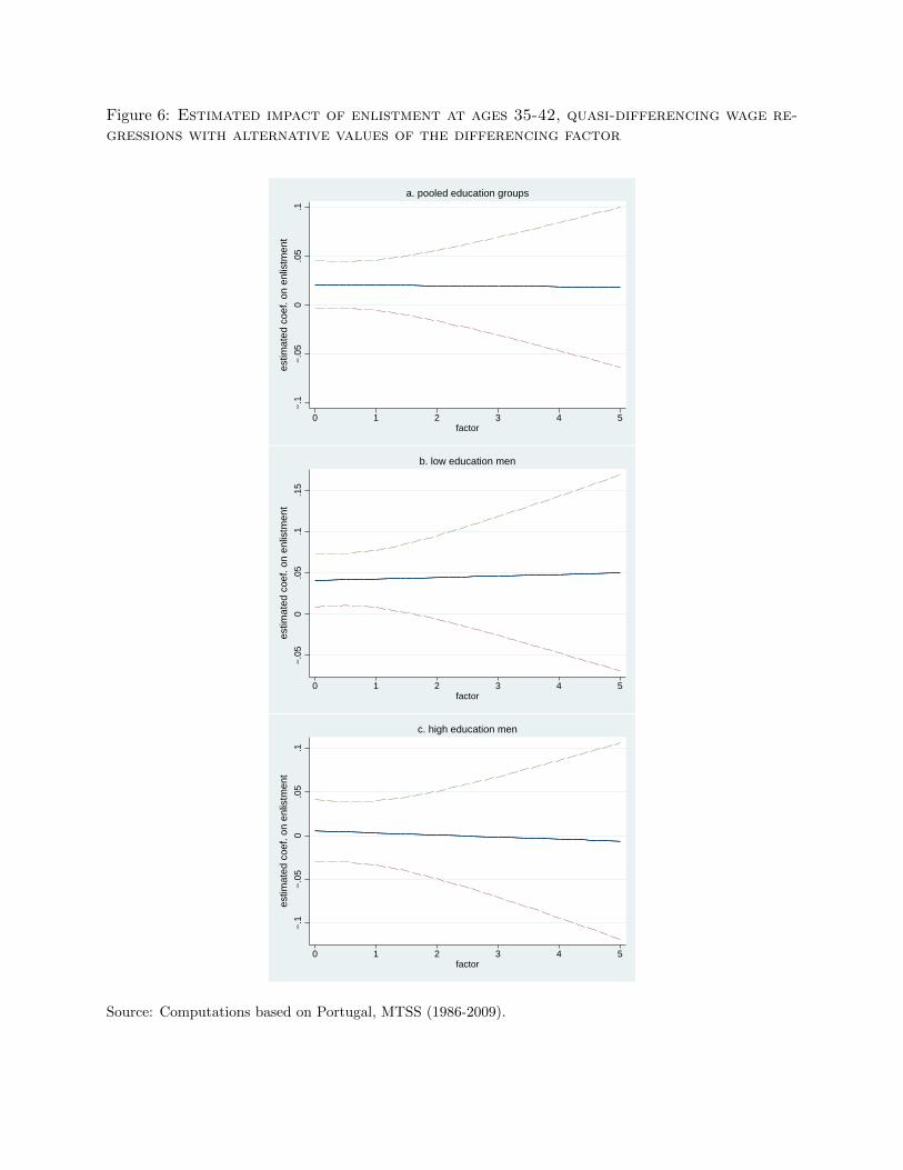
Figure 6: Estimated impact of enlistment at ages 35-42, quasi-differencing wage re-gressions with alternative values of the differencing factor

−.1

−.0

50

.05

.1

0 1 2 3 4 5factor

estim

ated

coe

f. on

enl

istm

ent

a. pooled education groups

−.0

50

.05

.1.1

5

0 1 2 3 4 5factor

estim

ated

coe

f. on

enl

istm

ent

b. low education men

−.1

−.0

50

.05

.1

0 1 2 3 4 5factor

estim

ated

coe

f. on

enl

istm

ent

c. high education men

Source: Computations based on Portugal, MTSS (1986-2009).