camera and laser robust integration in engineering and ...cdn.intechweb.org/pdfs/11663.pdfcamera and...
TRANSCRIPT

Camera and laser robust integration in engineering and architecture applications 115
Camera and laser robust integration in engineering and architecture applications
Pablo Rodriguez-Gonzalvez, Diego Gonzalez-Aguilera and Javier Gomez-Lahoz
X
Camera and laser robust integration in engineering and architecture applications
Pablo Rodriguez-Gonzalvez,
Diego Gonzalez-Aguilera and Javier Gomez-Lahoz Department of Cartographic and Land Engineering
High Polytechnic School of Avila, Spain University of Salamanca
1. Introduction
1.1 Motivation The 3D modelling of objects and complex scenes constitutes a field of multi-disciplinary research full of challenges and difficulties, ranging from the accuracy and reliability of the geometry, the radiometric quality of the results up to the portability and cost of the products, without forgetting the aim of automatization of the whole procedure. To this end, a wide variety of passive and active sensors are available of which the digital cameras and the scanner laser play the main role. Even though these two types of sensors can work in a separate fashion, it is when are merged together when the best results are attained. The following table (Table 1) gives an overview of the advantages and limitations of each technology. The comparison between the laser scanner and the digital camera (Table 1) stresses the incomplete character of the information derived from only one sensor. Therefore, we reach the conclusion that an integration of data sources and sensors must be achieved to improve the quality of procedures and results. Nevertheless, this sensor fusion poses a wide range of difficulties, derived not only from the different nature of the data (2D images and 3D scanner point clouds) but also from the different processing techniques related to the properties of each sensor. In this sense, an original sensor fusion approach is proposed and applied to the architecture and archaeology. This approach aims at achieving a high automatization level and provides high quality results all at once.
6
www.intechopen.com

Sensor Fusion and Its Applications116
Scanner laser Digital camera Not accurate extraction of lines High accuracy in the extraction of
lines Not visible junctions Visible junctions Colour information available on low resolution.
Colour information on high resolution
Straightforward access to metric information Awkward and slow access to metric information
High capacity and automatization in data capture
Less capacity and automatization in data capture
Data capture not immediate. Delays between scanning stations. Difficulties to move the equipment.
Flexibility and swiftness while handling the equipment.
Ability to render complex and irregular surfaces.
Limitations in the renderization of complex and irregular surfaces
High cost (60.000€-90.000€.) Low cost (From 100€) Not dependent on lighting conditions. Lighting conditions are demanding. ·3D model is a “cloud” without structure and topology.
The 3D model is accessed as a structured entity, including topology if desired.
Table 1. Comparison of advantages and drawbacks of laser scanner and digital camera.
1.2 State of the art The sensor fusion, in particular concerning the laser scanner and the digital camera, appears as a promising possibility to improve the data acquisition and the geometric and radiometric processing of these data. According to Mitka (2009), the sensor fusion may be divided in two general approaches: - On-site integration, that resides on a “physical” fusion of both sensors. This approach consists on a specific hardware structure that is previously calibrated. This solution provides a higher automatization and readiness in the data acquisition procedures but a higher dependency and a lack of flexibility in both the data acquisition and its processing. Examples of this kind of fusion are the commercial solutions of Trimble and Leica. Both are equipped with digital cameras that are housed in the inside of the device. These cameras exhibit a very poor resolution. (<1Mp). With the idea of accessing cameras with higher quality, other manufacturers present an exterior and calibrated frame to which a reflex camera can be attached. Faro Photon, Riegl LMS-Z620, Leica HDS6100 and Optech Ilris-3D are some of the laser systems that have incorporated this external sensor. Even though these approaches may lead to the idea that the sensor fusion is a straightforward question, the actual praxis is rather different, since the photos shoot time must be simultaneous to the scanning time, thus the illumination conditions as well as other conditions regarding the position of the camera or the environment may be far from the desired ones.
- Office integration, that consists on achieving the sensor fusion on laboratory, as the result of a processing procedure. This approach permits more flexibility in the data acquisition since it will not require neither a previously fixed and rigid framework nor a predetermined time of exposure. Nevertheless, this gain in flexibility demands the challenge of developing an automatic or semi-automatic procedure that aims at “tunning” both different data sources with different constructive fundamentals. According to Kong et al., (2007), the sensor fusion can be divided in three categories: the sensorial level (low level), the feature level (intermediate level) and the decision level (high level). In the sensorial level raw data are acquired from diverse sensors. This procedure is already solved for the onsite integration case but it is really complicated to afford when sensors are not calibrated to each other. In this sense, the question is to compute the rigid transformation (rotation and translation) that renders the relationship between both sensors, besides the camera model (camera calibration). The feature level merges the extraction and matching of several feature types. The procedure of feature extraction includes issues such as corners, interest points, borders and lines. These are extracted, labeled, located and matched through different algorithms. The decision level implies to take advantage of hybrid products derived from the processed data itself combined with the expert decision taking. Regarding the two first levels (sensorial and feature), several authors put forward the question of the fusion between the digital camera and the laser scanner through different approaches linked to different working environments. Levoy et al., (2000) in their project “Digital Michelangelo” carry on a camera pre-calibration facing integration with the laser scanner without any user interaction. In a similar context, Rocchini et al. (1999) obtain a fusion between the image and the laser model by means of an interactive selection of corresponding points. Nevertheless, both approaches are only applied to small objects such as sculptures and statues. With the idea of dealing with more complicated situations arising from complex scenes, Stamos and Allen, (2001) present an automatic fusion procedure between the laser model and the camera image. In this case, 3D lines are extracted by means of a segmentation procedure of the point clouds. After this, the 3D lines are matched with the borders extracted from the images. Some geometrical constraints, such as orthogonality and parallelism, that are common in urban scenes, are considered. In this way, this algorithm only works well in urban scenes where these conditions are met. In addition, the user must establish different kinds of thresholds in the segmentation process. All the above methodologies require the previous knowledge of the interior calibration parameters. With the aim of minimizing this drawback, Aguilera and Lahoz (2006) exploit a single view modelling to achieve an automatic fusion between a laser scanner and a not calibrated digital camera. Particularly, the question of the fusion between the two sensors is solved automatically through the search of 2D and 3D correspondences that are supported by the search of two spatial invariants: two distances and an angle. Nevertheless, some suppositions, such as the use of special targets and the presence of some geometric constraints on the image (vanishing points) are required to undertake the problem. More recently, Gonzalez-Aguilera et al. (2009) develop an automatic method to merge the digital image and the laser model by means of correspondences of the range image (laser) and the camera image. The main contribution of this approach resides on the use of a level hierarchy (pyramid) that takes advantage of the robust estimators, as well as of geometric constraints
www.intechopen.com

Camera and laser robust integration in engineering and architecture applications 117
Scanner laser Digital camera Not accurate extraction of lines High accuracy in the extraction of
lines Not visible junctions Visible junctions Colour information available on low resolution.
Colour information on high resolution
Straightforward access to metric information Awkward and slow access to metric information
High capacity and automatization in data capture
Less capacity and automatization in data capture
Data capture not immediate. Delays between scanning stations. Difficulties to move the equipment.
Flexibility and swiftness while handling the equipment.
Ability to render complex and irregular surfaces.
Limitations in the renderization of complex and irregular surfaces
High cost (60.000€-90.000€.) Low cost (From 100€) Not dependent on lighting conditions. Lighting conditions are demanding. ·3D model is a “cloud” without structure and topology.
The 3D model is accessed as a structured entity, including topology if desired.
Table 1. Comparison of advantages and drawbacks of laser scanner and digital camera.
1.2 State of the art The sensor fusion, in particular concerning the laser scanner and the digital camera, appears as a promising possibility to improve the data acquisition and the geometric and radiometric processing of these data. According to Mitka (2009), the sensor fusion may be divided in two general approaches: - On-site integration, that resides on a “physical” fusion of both sensors. This approach consists on a specific hardware structure that is previously calibrated. This solution provides a higher automatization and readiness in the data acquisition procedures but a higher dependency and a lack of flexibility in both the data acquisition and its processing. Examples of this kind of fusion are the commercial solutions of Trimble and Leica. Both are equipped with digital cameras that are housed in the inside of the device. These cameras exhibit a very poor resolution. (<1Mp). With the idea of accessing cameras with higher quality, other manufacturers present an exterior and calibrated frame to which a reflex camera can be attached. Faro Photon, Riegl LMS-Z620, Leica HDS6100 and Optech Ilris-3D are some of the laser systems that have incorporated this external sensor. Even though these approaches may lead to the idea that the sensor fusion is a straightforward question, the actual praxis is rather different, since the photos shoot time must be simultaneous to the scanning time, thus the illumination conditions as well as other conditions regarding the position of the camera or the environment may be far from the desired ones.
- Office integration, that consists on achieving the sensor fusion on laboratory, as the result of a processing procedure. This approach permits more flexibility in the data acquisition since it will not require neither a previously fixed and rigid framework nor a predetermined time of exposure. Nevertheless, this gain in flexibility demands the challenge of developing an automatic or semi-automatic procedure that aims at “tunning” both different data sources with different constructive fundamentals. According to Kong et al., (2007), the sensor fusion can be divided in three categories: the sensorial level (low level), the feature level (intermediate level) and the decision level (high level). In the sensorial level raw data are acquired from diverse sensors. This procedure is already solved for the onsite integration case but it is really complicated to afford when sensors are not calibrated to each other. In this sense, the question is to compute the rigid transformation (rotation and translation) that renders the relationship between both sensors, besides the camera model (camera calibration). The feature level merges the extraction and matching of several feature types. The procedure of feature extraction includes issues such as corners, interest points, borders and lines. These are extracted, labeled, located and matched through different algorithms. The decision level implies to take advantage of hybrid products derived from the processed data itself combined with the expert decision taking. Regarding the two first levels (sensorial and feature), several authors put forward the question of the fusion between the digital camera and the laser scanner through different approaches linked to different working environments. Levoy et al., (2000) in their project “Digital Michelangelo” carry on a camera pre-calibration facing integration with the laser scanner without any user interaction. In a similar context, Rocchini et al. (1999) obtain a fusion between the image and the laser model by means of an interactive selection of corresponding points. Nevertheless, both approaches are only applied to small objects such as sculptures and statues. With the idea of dealing with more complicated situations arising from complex scenes, Stamos and Allen, (2001) present an automatic fusion procedure between the laser model and the camera image. In this case, 3D lines are extracted by means of a segmentation procedure of the point clouds. After this, the 3D lines are matched with the borders extracted from the images. Some geometrical constraints, such as orthogonality and parallelism, that are common in urban scenes, are considered. In this way, this algorithm only works well in urban scenes where these conditions are met. In addition, the user must establish different kinds of thresholds in the segmentation process. All the above methodologies require the previous knowledge of the interior calibration parameters. With the aim of minimizing this drawback, Aguilera and Lahoz (2006) exploit a single view modelling to achieve an automatic fusion between a laser scanner and a not calibrated digital camera. Particularly, the question of the fusion between the two sensors is solved automatically through the search of 2D and 3D correspondences that are supported by the search of two spatial invariants: two distances and an angle. Nevertheless, some suppositions, such as the use of special targets and the presence of some geometric constraints on the image (vanishing points) are required to undertake the problem. More recently, Gonzalez-Aguilera et al. (2009) develop an automatic method to merge the digital image and the laser model by means of correspondences of the range image (laser) and the camera image. The main contribution of this approach resides on the use of a level hierarchy (pyramid) that takes advantage of the robust estimators, as well as of geometric constraints
www.intechopen.com

Sensor Fusion and Its Applications118
that ensure a higher accuracy and reliability. The data are processed and tested by means of software called USALign. Although there are many methodologies that try to progress in the fusion of both sensors taking advantage of the sensorial and the feature level, the radiometric and spectral properties of the sensors has not received enough attention. This issue is critical when the matching concerns images from different parts of the electromagnetic spectrum: visible (digital camera), near infrared (laser scanner) and medium/far infrared (thermal camera) and when the aspiration is to achieve an automatization of the whole procedure. Due to the different ways through which the pixel is formed, some methodologies developed for the visible image processing context may work in an inappropriate way or do not work at all. On this basis, this chapter on sensor fusion presents a method that has been developed and tested for the fusion of the laser scanner, the digital camera and the thermal camera. The structure of the chapter goes as follows: In the second part, we will tackle with the generalities related with the data acquisition and their pre-processing, concerning to the laser scanner, the digital camera and the thermal camera. In the third part, we will present the specific methodology based on a semi-automatic procedure supported by techniques of close range photogrammetry and computer vision. In the fourth part, a robust registration of sensors based on a spatial resection will be presented. In the fifth part, we will show the experimental results derived from the sensor fusion. A final part will devoted to the main conclusions and the expected future developments.
2. Pre-processing of data
In this section we will expose the treatment of the input data in order to prepare them for the established workflow.
2.1 Data Acquisition The acquisition protocol has been established with the greatest flexibility as possible in such a way that the method can be applied both to favourable and unfavourable cases. In this sense, the factors that will condition the level of difficulty will be:
Geometric complexity, directly related to the existence of complex forms as well as to the existence of occlusions.
Radiometric complexity, directly related to the spectral properties of each sensor, as well as to different illumination conditions of the scene.
Spatial and angular separation between sensors. The so called baseline will be a major factor when undertaking the correspondence between the sensors. This baseline will also condition the geometric and radiometric factors mentioned above. A short baseline will lead to images with a similar perspective view and consequently, to images easier to match and merge. On the contrary, a large baseline will produce images with big variations in perspective and so, with more difficulties for the correspondence. Nevertheless, rather than the length of the baseline, the critical factor will be the angle between the camera axis and the
average scanning direction. When this angle is large, the automatic fusion procedures will become difficult to undertake.
The following picture (Fig. 1) depicts the three questions mentioned above:
Fig. 1. Factors that influence the data acquisition with the laser scanner and the digital/thermal camera Through a careful planning of the acquisition framework, taking into account the issues referred before, some rules and basic principles should be stated (Mancera-Taboada et al., 2009). These could be particularised for the case studies analyzed in section 5 focussing on objects related to the architectural and archaeological field. In all of them the input data are the following: The point cloud is the input data in the case of the laser scanner and exhibits a 3D
character with specific metric and radiometric properties. Particularly, the cartesian coordinates XYZ associated to each of the points are accompanied by an intensity value associated to the energy of the return of each of the laser beams. The image that is formed from the point cloud, the range image, has radiometric properties derived from the wavelength of the electromagnetic spectrum, that is, the near or the medium infrared. This image depends on factors such as: the object material, the distance between the laser scanner and the object, the incidence angle between the scanner rays and the surface normal and the illumination of the scene. Also, in some cases, this value can be extended to a visible RGB colour value associated to each of the points.
The visible digital image is the input data coming from the digital camera and
presents a 2D character with specific metric and radiometric properties. Firstly, it is important that its geometric resolution must be in agreement with the object size and with the scanning resolution. The ideal would be that the number of elements in the point cloud would be the same that the number of pixels in the image. In this way, a perfect correspondence could be achieved between the image and the
www.intechopen.com

Camera and laser robust integration in engineering and architecture applications 119
that ensure a higher accuracy and reliability. The data are processed and tested by means of software called USALign. Although there are many methodologies that try to progress in the fusion of both sensors taking advantage of the sensorial and the feature level, the radiometric and spectral properties of the sensors has not received enough attention. This issue is critical when the matching concerns images from different parts of the electromagnetic spectrum: visible (digital camera), near infrared (laser scanner) and medium/far infrared (thermal camera) and when the aspiration is to achieve an automatization of the whole procedure. Due to the different ways through which the pixel is formed, some methodologies developed for the visible image processing context may work in an inappropriate way or do not work at all. On this basis, this chapter on sensor fusion presents a method that has been developed and tested for the fusion of the laser scanner, the digital camera and the thermal camera. The structure of the chapter goes as follows: In the second part, we will tackle with the generalities related with the data acquisition and their pre-processing, concerning to the laser scanner, the digital camera and the thermal camera. In the third part, we will present the specific methodology based on a semi-automatic procedure supported by techniques of close range photogrammetry and computer vision. In the fourth part, a robust registration of sensors based on a spatial resection will be presented. In the fifth part, we will show the experimental results derived from the sensor fusion. A final part will devoted to the main conclusions and the expected future developments.
2. Pre-processing of data
In this section we will expose the treatment of the input data in order to prepare them for the established workflow.
2.1 Data Acquisition The acquisition protocol has been established with the greatest flexibility as possible in such a way that the method can be applied both to favourable and unfavourable cases. In this sense, the factors that will condition the level of difficulty will be:
Geometric complexity, directly related to the existence of complex forms as well as to the existence of occlusions.
Radiometric complexity, directly related to the spectral properties of each sensor, as well as to different illumination conditions of the scene.
Spatial and angular separation between sensors. The so called baseline will be a major factor when undertaking the correspondence between the sensors. This baseline will also condition the geometric and radiometric factors mentioned above. A short baseline will lead to images with a similar perspective view and consequently, to images easier to match and merge. On the contrary, a large baseline will produce images with big variations in perspective and so, with more difficulties for the correspondence. Nevertheless, rather than the length of the baseline, the critical factor will be the angle between the camera axis and the
average scanning direction. When this angle is large, the automatic fusion procedures will become difficult to undertake.
The following picture (Fig. 1) depicts the three questions mentioned above:
Fig. 1. Factors that influence the data acquisition with the laser scanner and the digital/thermal camera Through a careful planning of the acquisition framework, taking into account the issues referred before, some rules and basic principles should be stated (Mancera-Taboada et al., 2009). These could be particularised for the case studies analyzed in section 5 focussing on objects related to the architectural and archaeological field. In all of them the input data are the following: The point cloud is the input data in the case of the laser scanner and exhibits a 3D
character with specific metric and radiometric properties. Particularly, the cartesian coordinates XYZ associated to each of the points are accompanied by an intensity value associated to the energy of the return of each of the laser beams. The image that is formed from the point cloud, the range image, has radiometric properties derived from the wavelength of the electromagnetic spectrum, that is, the near or the medium infrared. This image depends on factors such as: the object material, the distance between the laser scanner and the object, the incidence angle between the scanner rays and the surface normal and the illumination of the scene. Also, in some cases, this value can be extended to a visible RGB colour value associated to each of the points.
The visible digital image is the input data coming from the digital camera and
presents a 2D character with specific metric and radiometric properties. Firstly, it is important that its geometric resolution must be in agreement with the object size and with the scanning resolution. The ideal would be that the number of elements in the point cloud would be the same that the number of pixels in the image. In this way, a perfect correspondence could be achieved between the image and the
www.intechopen.com

Sensor Fusion and Its Applications120
point cloud and we could obtain the maximum performance from both data sets. In addition, for a given field of view for each sensor, we should seek that the whole object could be covered by a single image. As far as this cannot be achieved we should rely on an image mosaic where each image (previously processed) should be registered in an individual fashion. On the other hand, from a radiometric point of view, the images obtained from the digital camera should present a homogeneous illumination, avoiding, as far as it is possible, the high contrasts and any backlighting.
The thermal digital image is the input data coming from the thermal camera and presents a 2D character with specific metric and radiometric properties. From a geometric point of view they are low resolution images with the presence of high radial lens distortion. From a radiometric point of view the values distribution does not depend, as it does in the visible part of the electromagnetic spectrum, on the intensity gradient of the image that comes from part of the energy that is reflected by the object, but from the thermal gradient of the object itself as well as from the object emissivity. This represents a drawback in the fusion process.
2.2 Laser pre-processing Aiming to extrapolate part of the approaches that had already been applied to images by the protogrammetric and the computer vision communities, one of the first stages of the laser pre-processing will concern to the transformation of the point cloud into the range image.
2.2.1 Generation of a range image The range image generation process resides on the use of the collinearity equations (1) to project the points of the cloud over the image plane.
11 A S 12 A S 13 A SA
31 A S 32 A S 33 A S
21 A S 22 A S 23 A SA
31 A S 32 A S 33 A S
r (X X ) r (Y Y ) r (Z Z )x fr (X X ) r (Y Y ) r (Z Z )r (X X ) r (Y Y ) r (Z Z )y fr (X X ) r (Y Y ) r (Z Z )
(1)
To obtain the photo coordinates (xA,yA) of a three-dimensional point (XA,YA,ZA) the value of the exterior orientation parameters (XS,YS,ZS,,,), must have been computed. These are the target unknowns we address when we undertake the sensors registration procedure. As this is a question that must be solved through an iterative process, it becomes necessary to provide the system of equations (1) with a set of initial solutions that will stand for the exterior orientation of the virtual camera. The registration procedure will lead to a set of corrections in such a way that the final result will be the desired position and attitude. In this process it is necessary to define a focal length to perform the projection onto the range image. To achieve the best results and to preserve the initial configuration, the same focal length of the camera image will be chosen.
Fig. 2. Range-image generation from laser scanner point cloud Likewise, in the procedure of generation of the range-image a simple algorithm of visibility (depth correction) should be applied since there is a high probability that two or more points of the point cloud can be projected on the same image pixel, so an incorrect discrimination of the visible and occluded parts would hinder the appropriate application of the matching procedures (section 3). This visibility algorithm consists on storing, for every pixel, the radiometric value, as well as the distance between the projected point and optic virtual camera centre (both in the laser coordinate system). In this way, every time that a point cloud receives a pair of photo-coordinates, the new pair will be received only if the former point happens to be closer to the point of view than the latter (Straßer, 1974).
2.2.2 Texture Regeneration It is very common that the range image exhibits empty or white pixels because the object shape may lead to a non homogeneous distribution of the points in the cloud. Due to this, the perspective ray for a specific pixel may not intersect with a point in the cloud and consequently, it may happen that not all the points in the cloud have a correspondent point in the image. This lack of homogeneity in the range image texture drops the quality of the results in the matching processes because these are designed to work with the original conditions of real images. To overcome this drawback, the empty value of the pixel will be replaced by the value of some neighbouring pixels following an interpolation, based on distances (IDW - Inverse Distance Weighted) (Shepard, 1968). This method performs better than others because of its simplicity, efficiency and flexibility to adapt to swift changes in the data set. Its mathematical expression is
1
1
n
i ii
k n
ii
Z wZ
w (2)
www.intechopen.com

Camera and laser robust integration in engineering and architecture applications 121
point cloud and we could obtain the maximum performance from both data sets. In addition, for a given field of view for each sensor, we should seek that the whole object could be covered by a single image. As far as this cannot be achieved we should rely on an image mosaic where each image (previously processed) should be registered in an individual fashion. On the other hand, from a radiometric point of view, the images obtained from the digital camera should present a homogeneous illumination, avoiding, as far as it is possible, the high contrasts and any backlighting.
The thermal digital image is the input data coming from the thermal camera and presents a 2D character with specific metric and radiometric properties. From a geometric point of view they are low resolution images with the presence of high radial lens distortion. From a radiometric point of view the values distribution does not depend, as it does in the visible part of the electromagnetic spectrum, on the intensity gradient of the image that comes from part of the energy that is reflected by the object, but from the thermal gradient of the object itself as well as from the object emissivity. This represents a drawback in the fusion process.
2.2 Laser pre-processing Aiming to extrapolate part of the approaches that had already been applied to images by the protogrammetric and the computer vision communities, one of the first stages of the laser pre-processing will concern to the transformation of the point cloud into the range image.
2.2.1 Generation of a range image The range image generation process resides on the use of the collinearity equations (1) to project the points of the cloud over the image plane.
11 A S 12 A S 13 A SA
31 A S 32 A S 33 A S
21 A S 22 A S 23 A SA
31 A S 32 A S 33 A S
r (X X ) r (Y Y ) r (Z Z )x fr (X X ) r (Y Y ) r (Z Z )r (X X ) r (Y Y ) r (Z Z )y fr (X X ) r (Y Y ) r (Z Z )
(1)
To obtain the photo coordinates (xA,yA) of a three-dimensional point (XA,YA,ZA) the value of the exterior orientation parameters (XS,YS,ZS,,,), must have been computed. These are the target unknowns we address when we undertake the sensors registration procedure. As this is a question that must be solved through an iterative process, it becomes necessary to provide the system of equations (1) with a set of initial solutions that will stand for the exterior orientation of the virtual camera. The registration procedure will lead to a set of corrections in such a way that the final result will be the desired position and attitude. In this process it is necessary to define a focal length to perform the projection onto the range image. To achieve the best results and to preserve the initial configuration, the same focal length of the camera image will be chosen.
Fig. 2. Range-image generation from laser scanner point cloud Likewise, in the procedure of generation of the range-image a simple algorithm of visibility (depth correction) should be applied since there is a high probability that two or more points of the point cloud can be projected on the same image pixel, so an incorrect discrimination of the visible and occluded parts would hinder the appropriate application of the matching procedures (section 3). This visibility algorithm consists on storing, for every pixel, the radiometric value, as well as the distance between the projected point and optic virtual camera centre (both in the laser coordinate system). In this way, every time that a point cloud receives a pair of photo-coordinates, the new pair will be received only if the former point happens to be closer to the point of view than the latter (Straßer, 1974).
2.2.2 Texture Regeneration It is very common that the range image exhibits empty or white pixels because the object shape may lead to a non homogeneous distribution of the points in the cloud. Due to this, the perspective ray for a specific pixel may not intersect with a point in the cloud and consequently, it may happen that not all the points in the cloud have a correspondent point in the image. This lack of homogeneity in the range image texture drops the quality of the results in the matching processes because these are designed to work with the original conditions of real images. To overcome this drawback, the empty value of the pixel will be replaced by the value of some neighbouring pixels following an interpolation, based on distances (IDW - Inverse Distance Weighted) (Shepard, 1968). This method performs better than others because of its simplicity, efficiency and flexibility to adapt to swift changes in the data set. Its mathematical expression is
1
1
n
i ii
k n
ii
Z wZ
w (2)
www.intechopen.com

Sensor Fusion and Its Applications122
where Zk is the digital level of the empty pixel, Zi are the digital values of the neighbouring pixels, wi is the weighting factor and n is the number of points that are involved in the interpolation. Specifically this weighting factor is defined is the inverse of the square of distance between the pixel k and the i-th neighbouring pixel
2,
1ik i
wd
(3)
The neighbouring area is defined as a standard mask of 3x3 pixels, although this size may change depending on the image conditions. In this way, we ensure a correct interpolation within the empty pixels of the image according to its specific circumstances.
Fig. 3. Before (Left) and after (Right) the texture regeneration In (2) only one radiometric channel is addressed because the original point cloud data has only one channel (this is common for the intensity data) or because these data have been transformed from a RGB distribution in the original camera attached to the laser scanner to a single luminance value. At last, together with the creation of the range image, an equal size matrix is generated which stores the object coordinates corresponding to the point cloud. This matrix will be used in the sensor fusion procedure.
2.3 Pre-processing of the image The target of the pre-processing of the image that comes from the digital camera and/or from the thermal camera is to provide high quality radiometric information for the point cloud. Nevertheless, before reaching this point, it is necessary to pre-process the original image in order to make it in tune with the range image in the further procedures. In the following lines we will present the steps in this pre-processing task.
2.3.1 Determination and correction of the radial distortion One of the largest sources of error in the image is the existence of radial distortion. Particularly, in the context of the sensor fusion, the importance of the accurate determination and correction of the radial lens distortion resides in the fact that if this is not accurately corrected, we can expect that large displacements occur at the image edges, so this could lead to inadmissible errors in the matching process (Fig. 4).
Fig. 4. Displacement due to the radial distortion (Right): Real photo (Left), Ideal Photo (Centre) Please note in Fig. 4, how if the camera optical elements would be free from the radial distortion effects, the relationship between the image (2D) and the object (3D) would be linear, but such distortions are rather more complicated than this linear model and so, the transformation between image and object needs to account for this question. On the other hand, in the determination of the radial distortion we find that its modelling is far from being simple because, first of all, there is little agreement at the scientific community on the standard model to render this phenomenon and this leads to difficulties in the comparison and interpretation of the different models and so, it is not easy to assess the accuracy of the methodology. As a result empirical approaches are rather used (Sánchez et al., 2004). In our case, the radial distortion has been estimated by means of the so called Gaussian model as proposed by Brown (Brown, 1971). This model represents a “raw” determination of the radial distortion distribution and doses not account for any constraint to render the correlation between the focal length and such distribution(4).
3 51 2dr k r ' k r ' (4)
For the majority of the lenses and applications this polynomial can be reduced to the first term without a significant loss in accuracy. Particularly, the parameters k1 and k2 in the Gaussian model have been estimated by means of the software sv3DVision Aguilera and Lahoz (2006), which enables to estimate these parameters from a single image. To achieve this, it takes advantage of the existence of diverse geometrical constraints such as straight lines and vanishing points. In those cases of study, such as archaeological cases, in which these elements are scarce, the radial distortion parameters have been computed with the aid of the open-source software Fauccal (Douskos et al., 2009). Finally, it is important to state that the radial distortion parameters will require a constant updating, especially for consumer-grade compact cameras, since a lack of robustness and stability in their design will affect to the focal length stability. A detailed analysis of this question is developed by Sanz (2009) in its Ph.D thesis. Particularly, Sanz analysis as factors
www.intechopen.com

Camera and laser robust integration in engineering and architecture applications 123
where Zk is the digital level of the empty pixel, Zi are the digital values of the neighbouring pixels, wi is the weighting factor and n is the number of points that are involved in the interpolation. Specifically this weighting factor is defined is the inverse of the square of distance between the pixel k and the i-th neighbouring pixel
2,
1ik i
wd
(3)
The neighbouring area is defined as a standard mask of 3x3 pixels, although this size may change depending on the image conditions. In this way, we ensure a correct interpolation within the empty pixels of the image according to its specific circumstances.
Fig. 3. Before (Left) and after (Right) the texture regeneration In (2) only one radiometric channel is addressed because the original point cloud data has only one channel (this is common for the intensity data) or because these data have been transformed from a RGB distribution in the original camera attached to the laser scanner to a single luminance value. At last, together with the creation of the range image, an equal size matrix is generated which stores the object coordinates corresponding to the point cloud. This matrix will be used in the sensor fusion procedure.
2.3 Pre-processing of the image The target of the pre-processing of the image that comes from the digital camera and/or from the thermal camera is to provide high quality radiometric information for the point cloud. Nevertheless, before reaching this point, it is necessary to pre-process the original image in order to make it in tune with the range image in the further procedures. In the following lines we will present the steps in this pre-processing task.
2.3.1 Determination and correction of the radial distortion One of the largest sources of error in the image is the existence of radial distortion. Particularly, in the context of the sensor fusion, the importance of the accurate determination and correction of the radial lens distortion resides in the fact that if this is not accurately corrected, we can expect that large displacements occur at the image edges, so this could lead to inadmissible errors in the matching process (Fig. 4).
Fig. 4. Displacement due to the radial distortion (Right): Real photo (Left), Ideal Photo (Centre) Please note in Fig. 4, how if the camera optical elements would be free from the radial distortion effects, the relationship between the image (2D) and the object (3D) would be linear, but such distortions are rather more complicated than this linear model and so, the transformation between image and object needs to account for this question. On the other hand, in the determination of the radial distortion we find that its modelling is far from being simple because, first of all, there is little agreement at the scientific community on the standard model to render this phenomenon and this leads to difficulties in the comparison and interpretation of the different models and so, it is not easy to assess the accuracy of the methodology. As a result empirical approaches are rather used (Sánchez et al., 2004). In our case, the radial distortion has been estimated by means of the so called Gaussian model as proposed by Brown (Brown, 1971). This model represents a “raw” determination of the radial distortion distribution and doses not account for any constraint to render the correlation between the focal length and such distribution(4).
3 51 2dr k r ' k r ' (4)
For the majority of the lenses and applications this polynomial can be reduced to the first term without a significant loss in accuracy. Particularly, the parameters k1 and k2 in the Gaussian model have been estimated by means of the software sv3DVision Aguilera and Lahoz (2006), which enables to estimate these parameters from a single image. To achieve this, it takes advantage of the existence of diverse geometrical constraints such as straight lines and vanishing points. In those cases of study, such as archaeological cases, in which these elements are scarce, the radial distortion parameters have been computed with the aid of the open-source software Fauccal (Douskos et al., 2009). Finally, it is important to state that the radial distortion parameters will require a constant updating, especially for consumer-grade compact cameras, since a lack of robustness and stability in their design will affect to the focal length stability. A detailed analysis of this question is developed by Sanz (2009) in its Ph.D thesis. Particularly, Sanz analysis as factors
www.intechopen.com
Sensor Fusion and Its Applications124
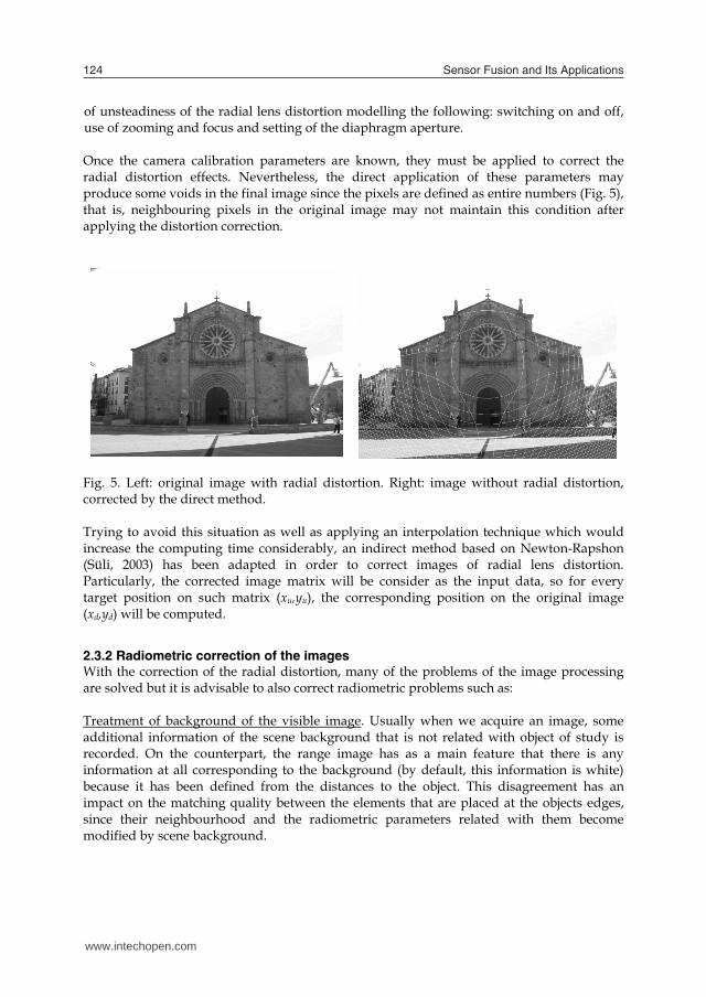
of unsteadiness of the radial lens distortion modelling the following: switching on and off, use of zooming and focus and setting of the diaphragm aperture. Once the camera calibration parameters are known, they must be applied to correct the radial distortion effects. Nevertheless, the direct application of these parameters may produce some voids in the final image since the pixels are defined as entire numbers (Fig. 5), that is, neighbouring pixels in the original image may not maintain this condition after applying the distortion correction.
Fig. 5. Left: original image with radial distortion. Right: image without radial distortion, corrected by the direct method. Trying to avoid this situation as well as applying an interpolation technique which would increase the computing time considerably, an indirect method based on Newton-Rapshon (Süli, 2003) has been adapted in order to correct images of radial lens distortion. Particularly, the corrected image matrix will be consider as the input data, so for every target position on such matrix (xu,yu), the corresponding position on the original image (xd,yd) will be computed.
2.3.2 Radiometric correction of the images With the correction of the radial distortion, many of the problems of the image processing are solved but it is advisable to also correct radiometric problems such as: Treatment of background of the visible image. Usually when we acquire an image, some additional information of the scene background that is not related with object of study is recorded. On the counterpart, the range image has as a main feature that there is any information at all corresponding to the background (by default, this information is white) because it has been defined from the distances to the object. This disagreement has an impact on the matching quality between the elements that are placed at the objects edges, since their neighbourhood and the radiometric parameters related with them become modified by scene background.
From all the elements that may appear at the background of an image shut at the outside (which is the case of the facades of architecture) the most common is the sky. This situation cannot be extrapolated to those elements in the inside or to those situations in which the illumination conditions are uniform (cloudy days), so this background correction would not be not necessary. Nevertheless, for the remaining cases in which the atmosphere appears clear, the background radiometry will be close to blue and, consequently it will turn necessary to proceed to its rejection. This is achieved thanks to its particular radiometric qualities. (Fig. 6).
Fig. 6. Before (Left) and after (Right) of rejecting the sky from camera image. The easiest and automatic way is to compute the blue channel in the original image, that is, to obtain an image whose digital levels are the third coordinate in the RGB space and to filter it depending on this value. The sky radiometry exhibits the largest values of blue component within the image (close to a digital level of 1, ranging from 0 to 1), and far away from the blue channel values that may present the facades of buildings (whose digital level usually spans from 0.4 to 0.8). Thus, we just have to implement a conditional instruction by which all pixels whose blue channel value is higher than a certain threshold, (this threshold being controlled by the user), will be substituted by white. Conversion of colour models: RGB->YUV. At this stage the RGB space radiometric information is transform into a scalar value of luminance. To achieve this, the YUV colour space is used because one of its main characteristics is that it is the model which renders more closely the human eye behaviour. This is done because the retina is more sensitive to the light intensity (luminance) than to the chromatic information. According to this, this space is defined by the three following components: Y (luminance component), U and V (chromatic components). The equation that relates the luminance of the YUV space with the coordinates of the RGB space is: Y 0, 299 R 0,587 G 0,114 B (5) Texture extraction. With the target of accomplishing a radiometric uniformity that supports the efficient treatment of the images (range, visible and thermal) in its intensity values, a region based texture extraction has been applied. The texture information extraction for purposes of image fusion has been scarcely treated in the scientific literature but some
www.intechopen.com

Camera and laser robust integration in engineering and architecture applications 125
of unsteadiness of the radial lens distortion modelling the following: switching on and off, use of zooming and focus and setting of the diaphragm aperture. Once the camera calibration parameters are known, they must be applied to correct the radial distortion effects. Nevertheless, the direct application of these parameters may produce some voids in the final image since the pixels are defined as entire numbers (Fig. 5), that is, neighbouring pixels in the original image may not maintain this condition after applying the distortion correction.
Fig. 5. Left: original image with radial distortion. Right: image without radial distortion, corrected by the direct method. Trying to avoid this situation as well as applying an interpolation technique which would increase the computing time considerably, an indirect method based on Newton-Rapshon (Süli, 2003) has been adapted in order to correct images of radial lens distortion. Particularly, the corrected image matrix will be consider as the input data, so for every target position on such matrix (xu,yu), the corresponding position on the original image (xd,yd) will be computed.
2.3.2 Radiometric correction of the images With the correction of the radial distortion, many of the problems of the image processing are solved but it is advisable to also correct radiometric problems such as: Treatment of background of the visible image. Usually when we acquire an image, some additional information of the scene background that is not related with object of study is recorded. On the counterpart, the range image has as a main feature that there is any information at all corresponding to the background (by default, this information is white) because it has been defined from the distances to the object. This disagreement has an impact on the matching quality between the elements that are placed at the objects edges, since their neighbourhood and the radiometric parameters related with them become modified by scene background.
From all the elements that may appear at the background of an image shut at the outside (which is the case of the facades of architecture) the most common is the sky. This situation cannot be extrapolated to those elements in the inside or to those situations in which the illumination conditions are uniform (cloudy days), so this background correction would not be not necessary. Nevertheless, for the remaining cases in which the atmosphere appears clear, the background radiometry will be close to blue and, consequently it will turn necessary to proceed to its rejection. This is achieved thanks to its particular radiometric qualities. (Fig. 6).
Fig. 6. Before (Left) and after (Right) of rejecting the sky from camera image. The easiest and automatic way is to compute the blue channel in the original image, that is, to obtain an image whose digital levels are the third coordinate in the RGB space and to filter it depending on this value. The sky radiometry exhibits the largest values of blue component within the image (close to a digital level of 1, ranging from 0 to 1), and far away from the blue channel values that may present the facades of buildings (whose digital level usually spans from 0.4 to 0.8). Thus, we just have to implement a conditional instruction by which all pixels whose blue channel value is higher than a certain threshold, (this threshold being controlled by the user), will be substituted by white. Conversion of colour models: RGB->YUV. At this stage the RGB space radiometric information is transform into a scalar value of luminance. To achieve this, the YUV colour space is used because one of its main characteristics is that it is the model which renders more closely the human eye behaviour. This is done because the retina is more sensitive to the light intensity (luminance) than to the chromatic information. According to this, this space is defined by the three following components: Y (luminance component), U and V (chromatic components). The equation that relates the luminance of the YUV space with the coordinates of the RGB space is: Y 0, 299 R 0,587 G 0,114 B (5) Texture extraction. With the target of accomplishing a radiometric uniformity that supports the efficient treatment of the images (range, visible and thermal) in its intensity values, a region based texture extraction has been applied. The texture information extraction for purposes of image fusion has been scarcely treated in the scientific literature but some
www.intechopen.com

Sensor Fusion and Its Applications126
experiments show that it could yield interesting results in those cases of low quality images (Rousseau et al., 2000; Jarc et al., 2007). The fusion procedure that has been developed will require, in particular, the texture extraction of thermal and range images. Usually, two filters are used for this type of task: Gabor (1946) or Laws (1980). In our case, we will use the Laws filter. Laws developed a set 2D convolution kernel filters which are composed by combinations of four one dimensional scalar filters. Each of these one dimensional filters will extract a particular feature from the image texture. These features are: level (L), edge (E), spot (S) and ripple (R). The one-dimensional kernels are as follows:
L5 1 4 6 4 1
E5 1 2 0 2 1
S5 1 0 2 0 1
R5 1 4 6 4 1
(6)
By the convolution of these kernels we get a set of 5x5 convolution kernels:
L5L5 E5L5 S5L5 R5L5L5E5 E5E5 S5E5 R5E5L5S5 E5S5 S5S5 R5S5L5R5 E5R5 S5R5 R5R5
(7)
The combination of these kernels gives 16 different filters. From them, and according to (Jarc, 2007), the more useful are E5L5, S5E5, S5L5 and their transposed. Particularly, considering that our cases of study related with thermal camera correspond to architectural buildings, the filters E5L5 and L5E5 have been applied in order to extract horizontal and vertical textures, respectively. Finally, each of the images filtered by the convolution kernels, were scaled for the range 0-255 and processed by histogram equalization and a contrast enhancement.
2.3.3 Image resizing In the last pre-processing images step, it is necessary to bring the existing images (range, visible and thermal) to a common frame to make them agreeable. Particularly, the visible image that comes from the digital camera usually will have a large size (7-10Mp), while the range image and the thermal image will have smaller sizes. The size of the range image will depend on the points of the laser cloud while the size of the thermal image depends on the low resolution of this sensor. Consequently, it is necessary to resize images in order to have a similar size (width and height) because, on the contrary, the matching algorithms would not be successful. An apparent solution would be to create a range and/or thermal image of the same size as the visible image. This solution presents an important drawback since in the case of the
range image this would demand to increase the number of points in the laser cloud and, in the case of the thermal image, the number of thermal pixels. Both solutions would require new data acquisition procedures that would rely on the increasing of the scanning resolution in the case of the range image and, in the case of the thermal image, on the generation of a mosaic from the original images. Both approaches have been disregarded for this work because they are not flexible enough for our purposes. We have chosen to resize all the images after they have been acquired and pre-processed seeking to achieve a balance between the number of pixels of the image with highest resolution (visible), the image with lowest resolution (thermal) and the number of laser points. The equation to render this sizing transformation is the 2D affine transformation (8).
Im g Im g
Im g Im g
b cd
0 0 1
1,2
R C
R T
A
1
2
A
A
ad e
(8)
where A1 contains the affine transformation between range image and camera image, A2 contains the affine transformation between range image and thermal image , and RImg, CImg y TImg are the matrices of range image, the visible image and the thermal image, respectively. After the resizing of the images we are prepared to start the sensor fusion.
3. Sensor fusion
One of the main targets of the fusion sensor strategy that we propose is the flexibility to use multiple sensors, so that the laser point cloud can be rendered with radiometric information and, vice versa, that the images can be enriched by the metric information provided by de laser scanner. Under this point of view, the sensor fusion processing that we will describe in the following pages will require extraction and matching approaches that can ensure: accuracy, reliability and unicity in the results.
3.1 Feature extraction The feature extraction that will be applied over the visible, range and thermal images must yield high quality in the results with a high level of automatization, so a good approximation for the matching process can be established. More specifically, the approach must ensure the robustness of the procedure in the case of repetitive radiometric patterns, which is usually the case when dealing with buildings. Even more, we must aim at guarantying the efficient feature extraction from images from different parts of the electromagnetic spectrum. To achieve this, we will use an interest point detector that
www.intechopen.com

Camera and laser robust integration in engineering and architecture applications 127
experiments show that it could yield interesting results in those cases of low quality images (Rousseau et al., 2000; Jarc et al., 2007). The fusion procedure that has been developed will require, in particular, the texture extraction of thermal and range images. Usually, two filters are used for this type of task: Gabor (1946) or Laws (1980). In our case, we will use the Laws filter. Laws developed a set 2D convolution kernel filters which are composed by combinations of four one dimensional scalar filters. Each of these one dimensional filters will extract a particular feature from the image texture. These features are: level (L), edge (E), spot (S) and ripple (R). The one-dimensional kernels are as follows:
L5 1 4 6 4 1
E5 1 2 0 2 1
S5 1 0 2 0 1
R5 1 4 6 4 1
(6)
By the convolution of these kernels we get a set of 5x5 convolution kernels:
L5L5 E5L5 S5L5 R5L5L5E5 E5E5 S5E5 R5E5L5S5 E5S5 S5S5 R5S5L5R5 E5R5 S5R5 R5R5
(7)
The combination of these kernels gives 16 different filters. From them, and according to (Jarc, 2007), the more useful are E5L5, S5E5, S5L5 and their transposed. Particularly, considering that our cases of study related with thermal camera correspond to architectural buildings, the filters E5L5 and L5E5 have been applied in order to extract horizontal and vertical textures, respectively. Finally, each of the images filtered by the convolution kernels, were scaled for the range 0-255 and processed by histogram equalization and a contrast enhancement.
2.3.3 Image resizing In the last pre-processing images step, it is necessary to bring the existing images (range, visible and thermal) to a common frame to make them agreeable. Particularly, the visible image that comes from the digital camera usually will have a large size (7-10Mp), while the range image and the thermal image will have smaller sizes. The size of the range image will depend on the points of the laser cloud while the size of the thermal image depends on the low resolution of this sensor. Consequently, it is necessary to resize images in order to have a similar size (width and height) because, on the contrary, the matching algorithms would not be successful. An apparent solution would be to create a range and/or thermal image of the same size as the visible image. This solution presents an important drawback since in the case of the
range image this would demand to increase the number of points in the laser cloud and, in the case of the thermal image, the number of thermal pixels. Both solutions would require new data acquisition procedures that would rely on the increasing of the scanning resolution in the case of the range image and, in the case of the thermal image, on the generation of a mosaic from the original images. Both approaches have been disregarded for this work because they are not flexible enough for our purposes. We have chosen to resize all the images after they have been acquired and pre-processed seeking to achieve a balance between the number of pixels of the image with highest resolution (visible), the image with lowest resolution (thermal) and the number of laser points. The equation to render this sizing transformation is the 2D affine transformation (8).
Im g Im g
Im g Im g
b cd
0 0 1
1,2
R C
R T
A
1
2
A
A
ad e
(8)
where A1 contains the affine transformation between range image and camera image, A2 contains the affine transformation between range image and thermal image , and RImg, CImg y TImg are the matrices of range image, the visible image and the thermal image, respectively. After the resizing of the images we are prepared to start the sensor fusion.
3. Sensor fusion
One of the main targets of the fusion sensor strategy that we propose is the flexibility to use multiple sensors, so that the laser point cloud can be rendered with radiometric information and, vice versa, that the images can be enriched by the metric information provided by de laser scanner. Under this point of view, the sensor fusion processing that we will describe in the following pages will require extraction and matching approaches that can ensure: accuracy, reliability and unicity in the results.
3.1 Feature extraction The feature extraction that will be applied over the visible, range and thermal images must yield high quality in the results with a high level of automatization, so a good approximation for the matching process can be established. More specifically, the approach must ensure the robustness of the procedure in the case of repetitive radiometric patterns, which is usually the case when dealing with buildings. Even more, we must aim at guarantying the efficient feature extraction from images from different parts of the electromagnetic spectrum. To achieve this, we will use an interest point detector that
www.intechopen.com

Sensor Fusion and Its Applications128
remains invariant to rotations and scale changes and an edge-line detector invariant to intensity variations on the images.
3.1.1 Extraction of interest points In the case of range and visible images two different interest points detectors, Harris (Harris y Stephen, 1988) and Förstner (Förstner and Guelch, 1987), have been considered since there is not an universal algorithm that provide ideal results for each situation. Obviously, the user always will have the opportunity to choose the interest point detector that considers more adequate. Harris operator provides stable and invariant spatial features that represent a good support for the matching process. This operator shows the following advantages when compared with other alternatives: high accuracy and reliability in the localization of interest points and invariance in the presence of noise. The threshold of the detector to assess the behaviour of the interest point is fixed as the relation between the eigenvector of the autocorrelation function of the kernel(9) and the standard deviation of the gaussian kernel. In addition, a non maximum elimination is applied to get the interest points:
2
1 2 1 2R k M k trace M (9) where R is the response parameter of the interest point, 1 y 2 are the eigenvectors of M, k is an empiric value and M is the auto-correlation matrix. If R is negative, the point is labeled as edge, if R is small is labeled as a planar region and if it is positive, the point is labeled as interest point. On the other hand, Förstner algorithm is one of the most widespread detectors in the field of terrestrial photogrammetry. Its performance (10) is based on analyzing the Hessian matrix and classifies the points as a point of interest based on the following parameters:
- The average precision of the point (w) - The direction of the major axis of the ellipse () - The form of the confidence ellipse (q)
2
22
41
1tr ( ) tr( )2
N NN N
1 2
1
λ λq w
λ λ (10)
where q is the ellipse circularity parameter, 1 and 2 are the eigenvalues of N, w the point weight and N the Hessian matrix. The use of q-parameter allows us to avoid the edges which are not suitable for the purposes of the present approach The recommended application of the selection criteria is as follows: firstly, remove those edges with a parameter (q) close to zero; next, check that the average precision of the point
(w) does not exceed the tolerance imposed by the user; finally, apply a non-maximum suppression to ensure that the confidence ellipse is the smallest in the neighbourhood.
3.1.2 Extraction of edges and lines The extraction of edges and lines is oriented to the fusion of the thermal and range images which present a large variation in their radiometry due to their spectral nature: near infrared or visible (green) for the laser scanner and far infrared for the thermal camera. In this sense, the edge and lines procedure follows a multiphase and hierarchical flux based on the Canny algorithm (Canny, 1986) and the latter segmentation of such edges by means of the Burns algorithm (Burns et al., 1986). Edge detection: Filter of Canny. The Canny edge detector is the most appropriate for the edge detection in images where there is a presence of regular elements because it meets three conditions that are determinant for our purposes:
Accuracy in the location of edge ensuring the largest closeness between the extracted edges and actual edges.
Reliability in the detection of the points in the edge, minimizing the probability of detecting false edges because of the presence of noise and, consequently, minimizing the loss of actual edges.
Unicity in the obtaining of a unique edge, ensuring edges with a maximum width of one pixel.
Mainly, the Canny edge detector filter consists of a multi-phase procedure in which the user must choose three parameters: a standard deviation and two threshold levels. The result will be a binary image in which the black pixels will indicate the edges while the rest of the pixels will be white.
Line segmentation: Burns. The linear segments of an image represent one of the most important features of the digital processing since they support the interpretation in three dimensions of the scene. Nevertheless, the segmentation procedure is not straightforward because the noise and the radial distortion will complicate its accomplishment. Achieving a high quality segmentation will demand to extract as limit points of the segment those that best define the line that can be adjusted to the edge. To meet so, the segmentation procedure that has been developed is, once more, structured on a multi-phase fashion in which a series of stages are chained pursuing to obtain a set of segments (1D) defined by their limit points coordinates. The processing time of the segmentation phase will linearly depend on the number of pixels that have been labeled as edge pixels in the previous phase. From here, it becomes crucial the choice of the three Canny parameters, described above.
The segmentation phase starts with the scanning of the edge image (from up to down and from left to right) seeking for candidate pixels to be labeled as belonging to the same line. The basic idea is to group the edge pixels according to similar gradient values, being this step similar to the Burns method. In this way, every pixel will be compared with its eight neighbours for each of the gradient directions. The pixels that show a similar orientation
www.intechopen.com

Camera and laser robust integration in engineering and architecture applications 129
remains invariant to rotations and scale changes and an edge-line detector invariant to intensity variations on the images.
3.1.1 Extraction of interest points In the case of range and visible images two different interest points detectors, Harris (Harris y Stephen, 1988) and Förstner (Förstner and Guelch, 1987), have been considered since there is not an universal algorithm that provide ideal results for each situation. Obviously, the user always will have the opportunity to choose the interest point detector that considers more adequate. Harris operator provides stable and invariant spatial features that represent a good support for the matching process. This operator shows the following advantages when compared with other alternatives: high accuracy and reliability in the localization of interest points and invariance in the presence of noise. The threshold of the detector to assess the behaviour of the interest point is fixed as the relation between the eigenvector of the autocorrelation function of the kernel(9) and the standard deviation of the gaussian kernel. In addition, a non maximum elimination is applied to get the interest points:
2
1 2 1 2R k M k trace M (9) where R is the response parameter of the interest point, 1 y 2 are the eigenvectors of M, k is an empiric value and M is the auto-correlation matrix. If R is negative, the point is labeled as edge, if R is small is labeled as a planar region and if it is positive, the point is labeled as interest point. On the other hand, Förstner algorithm is one of the most widespread detectors in the field of terrestrial photogrammetry. Its performance (10) is based on analyzing the Hessian matrix and classifies the points as a point of interest based on the following parameters:
- The average precision of the point (w) - The direction of the major axis of the ellipse () - The form of the confidence ellipse (q)
2
22
41
1tr ( ) tr( )2
N NN N
1 2
1
λ λq w
λ λ (10)
where q is the ellipse circularity parameter, 1 and 2 are the eigenvalues of N, w the point weight and N the Hessian matrix. The use of q-parameter allows us to avoid the edges which are not suitable for the purposes of the present approach The recommended application of the selection criteria is as follows: firstly, remove those edges with a parameter (q) close to zero; next, check that the average precision of the point
(w) does not exceed the tolerance imposed by the user; finally, apply a non-maximum suppression to ensure that the confidence ellipse is the smallest in the neighbourhood.
3.1.2 Extraction of edges and lines The extraction of edges and lines is oriented to the fusion of the thermal and range images which present a large variation in their radiometry due to their spectral nature: near infrared or visible (green) for the laser scanner and far infrared for the thermal camera. In this sense, the edge and lines procedure follows a multiphase and hierarchical flux based on the Canny algorithm (Canny, 1986) and the latter segmentation of such edges by means of the Burns algorithm (Burns et al., 1986). Edge detection: Filter of Canny. The Canny edge detector is the most appropriate for the edge detection in images where there is a presence of regular elements because it meets three conditions that are determinant for our purposes:
Accuracy in the location of edge ensuring the largest closeness between the extracted edges and actual edges.
Reliability in the detection of the points in the edge, minimizing the probability of detecting false edges because of the presence of noise and, consequently, minimizing the loss of actual edges.
Unicity in the obtaining of a unique edge, ensuring edges with a maximum width of one pixel.
Mainly, the Canny edge detector filter consists of a multi-phase procedure in which the user must choose three parameters: a standard deviation and two threshold levels. The result will be a binary image in which the black pixels will indicate the edges while the rest of the pixels will be white.
Line segmentation: Burns. The linear segments of an image represent one of the most important features of the digital processing since they support the interpretation in three dimensions of the scene. Nevertheless, the segmentation procedure is not straightforward because the noise and the radial distortion will complicate its accomplishment. Achieving a high quality segmentation will demand to extract as limit points of the segment those that best define the line that can be adjusted to the edge. To meet so, the segmentation procedure that has been developed is, once more, structured on a multi-phase fashion in which a series of stages are chained pursuing to obtain a set of segments (1D) defined by their limit points coordinates. The processing time of the segmentation phase will linearly depend on the number of pixels that have been labeled as edge pixels in the previous phase. From here, it becomes crucial the choice of the three Canny parameters, described above.
The segmentation phase starts with the scanning of the edge image (from up to down and from left to right) seeking for candidate pixels to be labeled as belonging to the same line. The basic idea is to group the edge pixels according to similar gradient values, being this step similar to the Burns method. In this way, every pixel will be compared with its eight neighbours for each of the gradient directions. The pixels that show a similar orientation
www.intechopen.com

Sensor Fusion and Its Applications130
will be labeled as belonging to the same edge: from here we will obtain a first clustering of the edges, according to their gradient. Finally, aiming at depurating and adapting the segmentation to our purposes, the edges resulting from the labeling stage will be filtered by means of the edge least length parameter. In our case, we want to extract only those most relevant lines to describe the object in order to find the most favourable features to support the matching process. To do so, the length of the labeled edges is computed and compared with a threshold length set by the user. If this length is larger than the threshold value the edge will be turned into a segment which will receive as limit coordinates the coordinates of the centre of the first and last pixel in the edge. On the contrary, if the length is smaller than the threshold level, the edge will be rejected (Fig. 7).
Fig. 7. Edge and line extraction with the Canny and Burns operators.
3.2 Matching Taking into account that the images present in the fusion problem (range, visible and thermal) are very different in their radiometry, we must undertake a robust strategy to ensure a unique solution. To this end, we will deal with two feature based matching strategies: the interest point based matching strategy (Li and Zouh, 1995; Lowe, 2005) and the edge and lines based matching strategy (Dana and Anandan, 1993; Keller and Averbuch, 2006), both integrated on a hierarchical and pyramidal procedure.
3.2.1 Interest Points Based Matching The interest point based matching will be used for the range and visible images fusion. To accomplish so, we have implemented a hierarchical matching strategy combining: correlation measures, matching, thresholding and geometrical constraints. Particularly, area-based and feature-based matching techniques have been used following the coarse-to-fine direction of the pyramid in such a way that the extracted interest points are matched among them according to their degree of similarity. At the lower levels of the pyramid, the matching task is developed through the closeness and grey level similarity within the neighbourhood. The area-based matching and cross-correlation coefficients are used as indicator (11).
HR
H R
(11)
where p is the cross-correlation coefficient, HR is the covariance between the windows of the visible image and the range image; H is the standard deviation of the visible image and y R is the standard deviation of the range image. The interest point based matching relays on closeness and similarity measures of the grey levels within the neighbourhood.
Later, at the last level of the pyramid, in which the image is processed at its real resolution the strategy will be based on the least squares matching (Grün, 1985). For this task, the initial approximations will be taken from the results of the area based matching applied on the previous levels. The localization and shape of the matching window is estimated from the initial values and recomputed until the differences between the grey levels comes to a minimum(12), min 0 0 0 0 1 0v F(x, y) G(ax by Δx cx dy Δy)r r (12)
where F and G represent the reference and the matching window respectively, a,b,c,d,x y y are the geometric parameters of an affine transformation while r1 and r0 are the radiometric parameters of a linear transformation, more precisely, the gain and the offset, respectively. Finally, even though the matching strategy has been applied in a hierarchical fashion, the particular radiometric properties of both images, especially the range image, may lead to many mismatches that would affect the results of the sensor fusion. Hence, the proposed approach has been reinforced including geometric constraints relying on the epipolar lines (Zhang et al., 1995; Han and Park, 2000). Particularly and taking into account the case of the laser scanner and the digital camera, given a 3D point in object space P, and being pr and pv its projections on the range and visible images, respectively and being Ol and Oc the origin of the laser scanner and the digital camera, respectively, we have that the plane defined by P, Ol and Oc is named the epipolar plane. The intersections of the epipolar plane with the range and visible image define the epipolar lines lr and lv. The location of an interest point on the range image pr, that matches a point pv on the visible image matching is constrained to lay at the epipolar line lr of the range image (Fig. 8). To compute these epipolarity constraints, the Fundamental Matrix is used (Hartley, 1997) using eight homologous points as input (Longuet-Higgins, 1981). In this way, once we have computed the Fundamental Matrix we can build the epipolar geometry and limit the search space for the matching points to one dimension: the epipolar line. As long as this strategy is an iterative process, the threshold levels to be applied in the matching task will vary in an adaptative way until we have reduced the search as much as possible and reach the maximum accuracy and reliability.
www.intechopen.com

Camera and laser robust integration in engineering and architecture applications 131
will be labeled as belonging to the same edge: from here we will obtain a first clustering of the edges, according to their gradient. Finally, aiming at depurating and adapting the segmentation to our purposes, the edges resulting from the labeling stage will be filtered by means of the edge least length parameter. In our case, we want to extract only those most relevant lines to describe the object in order to find the most favourable features to support the matching process. To do so, the length of the labeled edges is computed and compared with a threshold length set by the user. If this length is larger than the threshold value the edge will be turned into a segment which will receive as limit coordinates the coordinates of the centre of the first and last pixel in the edge. On the contrary, if the length is smaller than the threshold level, the edge will be rejected (Fig. 7).
Fig. 7. Edge and line extraction with the Canny and Burns operators.
3.2 Matching Taking into account that the images present in the fusion problem (range, visible and thermal) are very different in their radiometry, we must undertake a robust strategy to ensure a unique solution. To this end, we will deal with two feature based matching strategies: the interest point based matching strategy (Li and Zouh, 1995; Lowe, 2005) and the edge and lines based matching strategy (Dana and Anandan, 1993; Keller and Averbuch, 2006), both integrated on a hierarchical and pyramidal procedure.
3.2.1 Interest Points Based Matching The interest point based matching will be used for the range and visible images fusion. To accomplish so, we have implemented a hierarchical matching strategy combining: correlation measures, matching, thresholding and geometrical constraints. Particularly, area-based and feature-based matching techniques have been used following the coarse-to-fine direction of the pyramid in such a way that the extracted interest points are matched among them according to their degree of similarity. At the lower levels of the pyramid, the matching task is developed through the closeness and grey level similarity within the neighbourhood. The area-based matching and cross-correlation coefficients are used as indicator (11).
HR
H R
(11)
where p is the cross-correlation coefficient, HR is the covariance between the windows of the visible image and the range image; H is the standard deviation of the visible image and y R is the standard deviation of the range image. The interest point based matching relays on closeness and similarity measures of the grey levels within the neighbourhood.
Later, at the last level of the pyramid, in which the image is processed at its real resolution the strategy will be based on the least squares matching (Grün, 1985). For this task, the initial approximations will be taken from the results of the area based matching applied on the previous levels. The localization and shape of the matching window is estimated from the initial values and recomputed until the differences between the grey levels comes to a minimum(12), min 0 0 0 0 1 0v F(x, y) G(ax by Δx cx dy Δy)r r (12)
where F and G represent the reference and the matching window respectively, a,b,c,d,x y y are the geometric parameters of an affine transformation while r1 and r0 are the radiometric parameters of a linear transformation, more precisely, the gain and the offset, respectively. Finally, even though the matching strategy has been applied in a hierarchical fashion, the particular radiometric properties of both images, especially the range image, may lead to many mismatches that would affect the results of the sensor fusion. Hence, the proposed approach has been reinforced including geometric constraints relying on the epipolar lines (Zhang et al., 1995; Han and Park, 2000). Particularly and taking into account the case of the laser scanner and the digital camera, given a 3D point in object space P, and being pr and pv its projections on the range and visible images, respectively and being Ol and Oc the origin of the laser scanner and the digital camera, respectively, we have that the plane defined by P, Ol and Oc is named the epipolar plane. The intersections of the epipolar plane with the range and visible image define the epipolar lines lr and lv. The location of an interest point on the range image pr, that matches a point pv on the visible image matching is constrained to lay at the epipolar line lr of the range image (Fig. 8). To compute these epipolarity constraints, the Fundamental Matrix is used (Hartley, 1997) using eight homologous points as input (Longuet-Higgins, 1981). In this way, once we have computed the Fundamental Matrix we can build the epipolar geometry and limit the search space for the matching points to one dimension: the epipolar line. As long as this strategy is an iterative process, the threshold levels to be applied in the matching task will vary in an adaptative way until we have reduced the search as much as possible and reach the maximum accuracy and reliability.
www.intechopen.com

Sensor Fusion and Its Applications132
Fig. 8. Epipolar geometry used as geometric constraints in the matching process. In order to ensure the accuracy of the Fundamental Matrix, the iterative strategy has been supported by RANSAC algorithm (RANdom SAmpling Consensus) (Fischler and Bolles, 1981). This technique computes the mathematical model for a randomly selected dataset and evaluates the number of points of the global dataset which satisfy this model by a given threshold. The final accepted model will be that one which incorporates the larger set of points and the minimum error.
3.2.2 Line based matching The line based matching will be used for the range and thermal images fusion. Given the intrinsic properties of thermal image, it is not advisable to use the strategy outlined above since the radiometric response of thermal image is not related at all with the range image. This leads to a complication of the matching process when it is based on interest points and even to an ill-conditioned problem since a lot of interest points could not be matched. The solution proposed takes advantage of line based matching (Hintz & Zhao, 1990; Schenk, 1986) that exploits the direction criterion, distance criterion and attribute similarity criterion in a combined way. Nevertheless, this matching process is seriously limited by the ill-conditioning of both images: the correspondence can be of several lines to one (due to discontinuities), several lines regarded as independent may be part of the same, some lines may be wrong or may not exist at all (Luhmman et al., 2006). This is the reason for the pre-processing of these images according to a texture filtering (Laws, 1980) as described in the section (2.3.2). This will yield four images with a larger radiometric similarity degree and with horizontal and vertical textures extracted on which we can support our line based matching.
On the following lines we describe the three criteria we have applied for the line based matching: Direction criterion. We will take as an approach criterion to the line based matching the classification of these lines according to their direction. To this end, we take the edge orientation and the own gradient of the image as reference. The main goal in this first step is to classify the lines according to their horizontal and vertical direction, rejecting any other direction. In those cases in which we work with oblique images, a more sophisticated option could be applied to classify the linear segments according to the three main directions of the object (x,y,z) based on vanishing points (Gonzalez-Aguilera y Gomez-Lahoz, 2008). Distance criterion. Once we have classified the lines according to their direction we will take their distance attribute as the second criterion to search for the homologous line. Obviously, considering the different radiometric properties of both images, an adaptative threshold should be established since the distance of a matched line could present variations. Intersection criterion. In order to reinforce the matching of lines based on their distance, a specific strategy has been developed based on computing intersections between lines (corner points). Particularly, a buffer area (50x50 pixels) is defined where horizontal and vertical lines are enlarged to their intersection. In this sense, those lines that find a similar intersection points will be labelled as homologous lines. As a result of the application of these three criterions, a preliminary line based matching based on the fundamental matrix will be performed (see section 3.2.1). More precisely, the best eight intersections of lines matched perform as input data in the fundamental matrix. Once we have computed the Fundamental Matrix we can build the epipolar geometry and limit the search space for the matching lines to one dimension: the epipolar line. As long as this strategy is an iterative process, the threshold levels to be applied in the matching task will vary in an adaptative way until we have reduced the search as much as possible and reach the maximum accuracy and reliability.
4. Spatial resection
Once we have solved the matching task, through which we have related the images to each other (range image, visible image and thermal image) we proceed to solve the spatial resection. The parameters to be determined are the exterior parameters of the cameras (digital and thermal) respect of the laser scanner. The question of the spatial resection is well known on the classic aerial photogrammetry (Kraus, 1997). It is solved by the establishment of the relationship of the image points, the homologous object points and the point of view through a collinearity constraint (1). We must have in mind that the precision of the data on both systems (image and object) is different since their lineage is different, so we must write an adequate weighting for the stochastic model. This will lead to the so called unified approach to least squares adjustment (Mikhail and Ackerman, 1976) in the form:
www.intechopen.com

Camera and laser robust integration in engineering and architecture applications 133
Fig. 8. Epipolar geometry used as geometric constraints in the matching process. In order to ensure the accuracy of the Fundamental Matrix, the iterative strategy has been supported by RANSAC algorithm (RANdom SAmpling Consensus) (Fischler and Bolles, 1981). This technique computes the mathematical model for a randomly selected dataset and evaluates the number of points of the global dataset which satisfy this model by a given threshold. The final accepted model will be that one which incorporates the larger set of points and the minimum error.
3.2.2 Line based matching The line based matching will be used for the range and thermal images fusion. Given the intrinsic properties of thermal image, it is not advisable to use the strategy outlined above since the radiometric response of thermal image is not related at all with the range image. This leads to a complication of the matching process when it is based on interest points and even to an ill-conditioned problem since a lot of interest points could not be matched. The solution proposed takes advantage of line based matching (Hintz & Zhao, 1990; Schenk, 1986) that exploits the direction criterion, distance criterion and attribute similarity criterion in a combined way. Nevertheless, this matching process is seriously limited by the ill-conditioning of both images: the correspondence can be of several lines to one (due to discontinuities), several lines regarded as independent may be part of the same, some lines may be wrong or may not exist at all (Luhmman et al., 2006). This is the reason for the pre-processing of these images according to a texture filtering (Laws, 1980) as described in the section (2.3.2). This will yield four images with a larger radiometric similarity degree and with horizontal and vertical textures extracted on which we can support our line based matching.
On the following lines we describe the three criteria we have applied for the line based matching: Direction criterion. We will take as an approach criterion to the line based matching the classification of these lines according to their direction. To this end, we take the edge orientation and the own gradient of the image as reference. The main goal in this first step is to classify the lines according to their horizontal and vertical direction, rejecting any other direction. In those cases in which we work with oblique images, a more sophisticated option could be applied to classify the linear segments according to the three main directions of the object (x,y,z) based on vanishing points (Gonzalez-Aguilera y Gomez-Lahoz, 2008). Distance criterion. Once we have classified the lines according to their direction we will take their distance attribute as the second criterion to search for the homologous line. Obviously, considering the different radiometric properties of both images, an adaptative threshold should be established since the distance of a matched line could present variations. Intersection criterion. In order to reinforce the matching of lines based on their distance, a specific strategy has been developed based on computing intersections between lines (corner points). Particularly, a buffer area (50x50 pixels) is defined where horizontal and vertical lines are enlarged to their intersection. In this sense, those lines that find a similar intersection points will be labelled as homologous lines. As a result of the application of these three criterions, a preliminary line based matching based on the fundamental matrix will be performed (see section 3.2.1). More precisely, the best eight intersections of lines matched perform as input data in the fundamental matrix. Once we have computed the Fundamental Matrix we can build the epipolar geometry and limit the search space for the matching lines to one dimension: the epipolar line. As long as this strategy is an iterative process, the threshold levels to be applied in the matching task will vary in an adaptative way until we have reduced the search as much as possible and reach the maximum accuracy and reliability.
4. Spatial resection
Once we have solved the matching task, through which we have related the images to each other (range image, visible image and thermal image) we proceed to solve the spatial resection. The parameters to be determined are the exterior parameters of the cameras (digital and thermal) respect of the laser scanner. The question of the spatial resection is well known on the classic aerial photogrammetry (Kraus, 1997). It is solved by the establishment of the relationship of the image points, the homologous object points and the point of view through a collinearity constraint (1). We must have in mind that the precision of the data on both systems (image and object) is different since their lineage is different, so we must write an adequate weighting for the stochastic model. This will lead to the so called unified approach to least squares adjustment (Mikhail and Ackerman, 1976) in the form:
www.intechopen.com

Sensor Fusion and Its Applications134
L BV AX 0 (13) where L is the independent term vector, B is the jacobian matrix of the observations, V is the vector of the residuals, A is the jacobian matrix of the unknowns and X is the vector of unknowns. The normal equation system we get after applying the criterion of least squares is in the form:
T 1 T 1 1 TA M Ax A M L 0 where M BW B (14)
This equation is equivalent to the least squares solution we obtain when directly solving for the so called observation equation system. In this case we can say that the matrix M plays the role of weighting the equations (instead of the observations). Please note that this matrix is obtained from the weighting of the observations (through the matrix W) and from the functional relationship among them expressed the jacobian matrix (matrix B). In this way, this matrix operates in the equation system as a geometrical counterpart of the metrical relationship between the precision of the different observations (image and object). From the equation (13) and its solution (14) we can obtain the adjusted residuals:
11 T 1 TV W B BW B AX L (15)
According to the covariance propagation law (Mikhail and Ackermann, 1976), the cofactor matrix of the estimated parameters is obtained from the equation:
1 1 1T 1 T 1 1 T 1 T 1
x̂ L
1 TL
Q A M A A M Q M A A M A A M A
Q BW B M
(16)
and so, the covariance matrix of the spatial resection is given by:
2ˆ ˆx 0 xC Q (17)
The square root of the elements in the main diagonal of the matrix provides the standard deviation of the exterior orientation parameters. Finally, the mean square error is obtained from:
TV WV
e.m.c.2n 6
(18)
On the other side, with the aim of comparing the results and analyzing its validity we have also solved the spatial resection by means of the so called Direct Linear Transformation
(DLT) (Abdel-Aziz, 1971). This method represented and innovation in phtogrammetry because allow us to relate the instrumental coordinates with the object coordinates without undertaking the intermediate steps (interior and exterior orientation). This approach allows us to solve without knowing camera parameters (focal length and principal point position) making the procedure especially interesting for non-metric cameras. Another advantage is that it could be solved as a linear model and thus, avoiding the iterative approach and the need of providing initial approximations for the unknowns The DLT equations results from a re-parameterization of the collinearity equations (Kraus, 1997) in the following way,
A p A S
A p A S
A S
x x X Xy y R Y Y
f Z Z
(19)
in which (XS,YS,ZS) are the object coordinates of the point of view, (XA,YA,ZA) are the object coordinates of an object point and (xA,yA) are the image coordinates of an image point homologous of the first, f is the focal length, (xp,yp) are the image coordinates of the principal point, R is the 3x3 rotation matrix and is the scale factor. If we expand the terms and divide the equations among them to eliminate the scale factor we have:
p 31 11 A p 32 12 A p 33 13 A p 31 11 S p 32 12 S p 33 13 S
A
31 A 32 A 33 A 31 S 32 S 33 S
p 31 21 A p 32 22 A p 33 23 A p 31 21 S p 32 22 S p 33 23 S
A
31 A
x r fr X x r fr Y x r fr Z x r fr X x r fr Y x r fr Zx
r X r Y r Z r X r Y r Z
y r fr X y r fr Y y r fr Z y r fr X y r fr Y y r fr Zy
r X
32 A 33 A 31 S 32 S 33 Sr Y r Z r X r Y r Z
(20)
Rearranging and renaming, we finally get the DLT expression:
1 2 3 4 5 6 7 8
9 10 11 9 10 11
A A A A A AA A
A A A A A A
L X L Y L Z L L X L Y L Z Lx y
L X L Y L Z 1 L X L Y L Z 1 (21)
This expression relates image coordinates (xA,yA) with the object coordinates (XA,YA,ZA), and consequently, it is useful to reference the images to the laser model. The relationship between the mathematical parameters (L1,…,L11) and the geometrical parameters is as follows:
www.intechopen.com
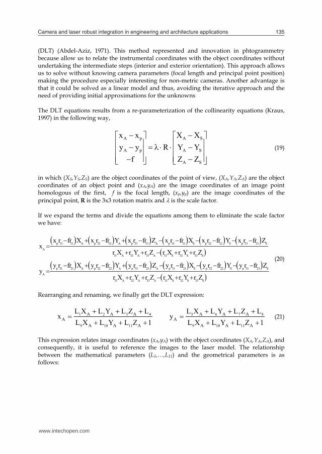
Camera and laser robust integration in engineering and architecture applications 135
L BV AX 0 (13) where L is the independent term vector, B is the jacobian matrix of the observations, V is the vector of the residuals, A is the jacobian matrix of the unknowns and X is the vector of unknowns. The normal equation system we get after applying the criterion of least squares is in the form:
T 1 T 1 1 TA M Ax A M L 0 where M BW B (14)
This equation is equivalent to the least squares solution we obtain when directly solving for the so called observation equation system. In this case we can say that the matrix M plays the role of weighting the equations (instead of the observations). Please note that this matrix is obtained from the weighting of the observations (through the matrix W) and from the functional relationship among them expressed the jacobian matrix (matrix B). In this way, this matrix operates in the equation system as a geometrical counterpart of the metrical relationship between the precision of the different observations (image and object). From the equation (13) and its solution (14) we can obtain the adjusted residuals:
11 T 1 TV W B BW B AX L (15)
According to the covariance propagation law (Mikhail and Ackermann, 1976), the cofactor matrix of the estimated parameters is obtained from the equation:
1 1 1T 1 T 1 1 T 1 T 1
x̂ L
1 TL
Q A M A A M Q M A A M A A M A
Q BW B M
(16)
and so, the covariance matrix of the spatial resection is given by:
2ˆ ˆx 0 xC Q (17)
The square root of the elements in the main diagonal of the matrix provides the standard deviation of the exterior orientation parameters. Finally, the mean square error is obtained from:
TV WV
e.m.c.2n 6
(18)
On the other side, with the aim of comparing the results and analyzing its validity we have also solved the spatial resection by means of the so called Direct Linear Transformation
(DLT) (Abdel-Aziz, 1971). This method represented and innovation in phtogrammetry because allow us to relate the instrumental coordinates with the object coordinates without undertaking the intermediate steps (interior and exterior orientation). This approach allows us to solve without knowing camera parameters (focal length and principal point position) making the procedure especially interesting for non-metric cameras. Another advantage is that it could be solved as a linear model and thus, avoiding the iterative approach and the need of providing initial approximations for the unknowns The DLT equations results from a re-parameterization of the collinearity equations (Kraus, 1997) in the following way,
A p A S
A p A S
A S
x x X Xy y R Y Y
f Z Z
(19)
in which (XS,YS,ZS) are the object coordinates of the point of view, (XA,YA,ZA) are the object coordinates of an object point and (xA,yA) are the image coordinates of an image point homologous of the first, f is the focal length, (xp,yp) are the image coordinates of the principal point, R is the 3x3 rotation matrix and is the scale factor. If we expand the terms and divide the equations among them to eliminate the scale factor we have:
p 31 11 A p 32 12 A p 33 13 A p 31 11 S p 32 12 S p 33 13 S
A
31 A 32 A 33 A 31 S 32 S 33 S
p 31 21 A p 32 22 A p 33 23 A p 31 21 S p 32 22 S p 33 23 S
A
31 A
x r fr X x r fr Y x r fr Z x r fr X x r fr Y x r fr Zx
r X r Y r Z r X r Y r Z
y r fr X y r fr Y y r fr Z y r fr X y r fr Y y r fr Zy
r X
32 A 33 A 31 S 32 S 33 Sr Y r Z r X r Y r Z
(20)
Rearranging and renaming, we finally get the DLT expression:
1 2 3 4 5 6 7 8
9 10 11 9 10 11
A A A A A AA A
A A A A A A
L X L Y L Z L L X L Y L Z Lx y
L X L Y L Z 1 L X L Y L Z 1 (21)
This expression relates image coordinates (xA,yA) with the object coordinates (XA,YA,ZA), and consequently, it is useful to reference the images to the laser model. The relationship between the mathematical parameters (L1,…,L11) and the geometrical parameters is as follows:
www.intechopen.com

Sensor Fusion and Its Applications136
p 31 11 p 32 12
1 2
31 S
p 33 133
11 p 31 S 12 p 32 S 13 p 33 S4
p 31 21 p 32 22 p 33 235 6 7
21 p 31 S 22 p 32 S 23 p 33 S8
31 32 339 10 11
x r fr x r frL L
D D
D r X
x r frL
Dfr x r X fr x r Y fr x r Z
LD
y r fr y r fr y r frL L L
D D Dfr y r X fr y r Y fr y r Z
LD
r r rL L L
D D D
32 S 33 Sr Y r Z
(22)
The inverse relationship is:
1
S 1 2 3 4
S 5 6 7 8
S 9 10 11
1 9 2 10 3 11p 2 2 2
9 10 11
5 9 6 10 7 11p 2 2 2
9 10 11
p 9 1 p 10 2 p 11 3
11 12 13
21 22 23
31 32 33
X L L L LY L L L LZ L L L 1
L L L L L Lx
L L L
L L L L L Ly
L L L
x L L x L L x L L
f f fr r ry
R r r r Dr r r
p 9 5 p 10 6 p 10 7
9 10 11
22 2 29 10 11
L L y L L y L L
f f fL L L
1D
L L L
(23)
To solve the spatial resection both models are effective. Nevertheless, some differences must be remarked:
- DLT is a linear model and therefore it does not require neither an iterative process nor initial values for the first iteration (both derived from de Taylor series expansion).
- The number of parameters to be solved when using the DLT is 11 and so, we need at least to have measured 6 control points (2 equations for each point) whereas the number of parameters to be solved when using the collinearity equations is directly 6 (if we are only solving for the exterior orientation or 9 (if we are solving for the exterior orientation and for the three parameters of the interior orientation that the describe the camera without taking into account any systematic error such a as radial lens distortion). Therefore, we will need three control points in the first case, and five in the second case.
Concerning the reliability of the spatial resection, it is important to stress that in spite of robust computing methods that we have applied at the matching stage, there may still persist some mismatching on the candidates homologous points and so the final accuracy could be reduced. These blunders are not easy to detect because in the adjustment its influence is distributed over all the points. As is well known, the least squares approach allows to detect blunders when the geometry is robust, that is, when the conditioning of the design matrix A is good but when the geometry design is weak the high residual which should be related with the gross error is distributed over other residuals. Consequently, it becomes necessary to apply statistical tests such as the Test of Baarda (Baarda, 1968), and/or the Test of Pope (Pope, 1976), as well as robust estimators that can detect and eliminate such wrong observations. Regarding the statistical tests, they are affected by some limitations, some of which are related with the workflow described up to here. These are:
If the data set present a bias, that is, the errors do not follow a gaussian distribution the statistical tests will lose a large part of its performance
Form the actual set of available statistical tests, only the test of Pope can work without knowing previously the variance of the observations. Unfortunately, this is usually the case in photogrammetry.
As stated before, in the case of working under a weak geometry, the probability that these tests do not perform adequately greatly increases. In addition, these tests are only able of rejecting one observation at each iteration.
On the contrary, these statistical tests exhibit the advantage that they may be applied in a fully automated fashion, and thus avoiding the interaction with the user. The test of Baarda (Baarda, 1968), assumes that the theoretical variance is not known and therefore will use the a priori variance (02). It also works on the assumption that the standard deviation of the observations is known. The test is based on the fact that the residuals are normally (gaussian) distributed. The test indicator is the normalised residual (zi), defined as:
i
i0 vv ii
Pvz
PQ P (24)
www.intechopen.com

Camera and laser robust integration in engineering and architecture applications 137
p 31 11 p 32 12
1 2
31 S
p 33 133
11 p 31 S 12 p 32 S 13 p 33 S4
p 31 21 p 32 22 p 33 235 6 7
21 p 31 S 22 p 32 S 23 p 33 S8
31 32 339 10 11
x r fr x r frL L
D D
D r X
x r frL
Dfr x r X fr x r Y fr x r Z
LD
y r fr y r fr y r frL L L
D D Dfr y r X fr y r Y fr y r Z
LD
r r rL L L
D D D
32 S 33 Sr Y r Z
(22)
The inverse relationship is:
1
S 1 2 3 4
S 5 6 7 8
S 9 10 11
1 9 2 10 3 11p 2 2 2
9 10 11
5 9 6 10 7 11p 2 2 2
9 10 11
p 9 1 p 10 2 p 11 3
11 12 13
21 22 23
31 32 33
X L L L LY L L L LZ L L L 1
L L L L L Lx
L L L
L L L L L Ly
L L L
x L L x L L x L L
f f fr r ry
R r r r Dr r r
p 9 5 p 10 6 p 10 7
9 10 11
22 2 29 10 11
L L y L L y L L
f f fL L L
1D
L L L
(23)
To solve the spatial resection both models are effective. Nevertheless, some differences must be remarked:
- DLT is a linear model and therefore it does not require neither an iterative process nor initial values for the first iteration (both derived from de Taylor series expansion).
- The number of parameters to be solved when using the DLT is 11 and so, we need at least to have measured 6 control points (2 equations for each point) whereas the number of parameters to be solved when using the collinearity equations is directly 6 (if we are only solving for the exterior orientation or 9 (if we are solving for the exterior orientation and for the three parameters of the interior orientation that the describe the camera without taking into account any systematic error such a as radial lens distortion). Therefore, we will need three control points in the first case, and five in the second case.
Concerning the reliability of the spatial resection, it is important to stress that in spite of robust computing methods that we have applied at the matching stage, there may still persist some mismatching on the candidates homologous points and so the final accuracy could be reduced. These blunders are not easy to detect because in the adjustment its influence is distributed over all the points. As is well known, the least squares approach allows to detect blunders when the geometry is robust, that is, when the conditioning of the design matrix A is good but when the geometry design is weak the high residual which should be related with the gross error is distributed over other residuals. Consequently, it becomes necessary to apply statistical tests such as the Test of Baarda (Baarda, 1968), and/or the Test of Pope (Pope, 1976), as well as robust estimators that can detect and eliminate such wrong observations. Regarding the statistical tests, they are affected by some limitations, some of which are related with the workflow described up to here. These are:
If the data set present a bias, that is, the errors do not follow a gaussian distribution the statistical tests will lose a large part of its performance
Form the actual set of available statistical tests, only the test of Pope can work without knowing previously the variance of the observations. Unfortunately, this is usually the case in photogrammetry.
As stated before, in the case of working under a weak geometry, the probability that these tests do not perform adequately greatly increases. In addition, these tests are only able of rejecting one observation at each iteration.
On the contrary, these statistical tests exhibit the advantage that they may be applied in a fully automated fashion, and thus avoiding the interaction with the user. The test of Baarda (Baarda, 1968), assumes that the theoretical variance is not known and therefore will use the a priori variance (02). It also works on the assumption that the standard deviation of the observations is known. The test is based on the fact that the residuals are normally (gaussian) distributed. The test indicator is the normalised residual (zi), defined as:
i
i0 vv ii
Pvz
PQ P (24)
www.intechopen.com

Sensor Fusion and Its Applications138
where P is the matrix of weights, vi is the i-th residual, and Qvv is the cofactor matrix of the residuals. This indicator is compared with the critical value of the test to accept or reject the null hypothesis (H0). It is defined by:
2b 2 1, , 1, ,T N F (25)
Where is the significance level, N represents the normal distribution, F is the distribution of Fischer-Snedecor and is the Square – Chi table. The critical value of Baarda (Tb) takes into account the level of significance as well as the power of the test. Therefore, it is very common that certain combinations of and are used in the majority of cases. The most common is =0,1 % and =20%, which leads to a critical value of 3,291. If the null hypothesis is rejected, we will assume that there is gross error among the observations. Therefore, the procedure will consist on eliminating from the adjustment the point with the largest typified residual and repeating the test of Baarda to check if there are more gross errors. The iterative application of this strategy is called data snooping (Kraus, 1997) and permits to detect multiple blunders and to reject them from the adjustment. The test of Pope (Pope, 1976) is used when the a priori variance (02) is not known or is not possible to be determined. In its place the a posteriori variance (26) is used.
T
20
V PVˆr
(26)
This statistic test is usually applied in Photogrammetry since it is very common that the a priori variance is not known. The null hypothesis (H0) is that all the residuals (vi) follow a normal (gaussian) distribution N(0,) such that its variance is the residual normalized variance.
i
ˆ 0 iiVˆ q (27)
where qvivi is the i.th element of the main diagonal of the cofactor matrix of the residuals (Qvv). On the contrary, the alternative hypothesis (Ha) states that the in the set of observations there is a gross error that does not behave according to the normal distribution and, thus, must be eliminated. Thus, we establish as statistical indicator the standardised residuals (wi) that is obtained as:
ii
0 Vi
vwˆ
(28)
Please note that in this test we use the standardised residuals (wi), while in the test of Baarda we use the normalised residual (zi). The only difference is the use of the a posteriori and a priori variance, respectively. Since the residuals are computed using the a posteriori variance they will not be normally distributed (25)but rather will follow a Tau distribution. The critical value of the Tau distribution may be computed from the tables of the t-student distribution (Heck, 1981) according to:
0
0
0
2
r 1, 2r, 2, 2
r 1, 2
r t
r 1 t
(29)
where r are the degree of freedom of the adjustment and 0 the significance level for a single observation that is computing from the total significance level () and the number of observations (n):
1n
0 1 1n
(30)
If the alternative hypothesis is accepted, the standardised residual wi will be regarded as a blunder and hence will be eliminated from the adjustment. The procedure is repeated until the null hypothesis is verified for all the remaining points in a similar way as has been done with the data snooping technique, described above. In addition to the statistical tests described before it is possible (and recommended) to include in the parameter computation a robust estimator to complete the least squares technique. While the base for the statistical estimators is the progressive suppression of the gross errors, the robust estimators technique sets a low weighting of the bad observations and keeps them in the adjustment. These weights depend on the inverse of the magnitude of the residual itself and so error the bad observations are “punished” with low weights which leads in time to a worse residual and to lower weight. The main feature of the robust estimators is they minimize a function different than the sum of squares of the residuals and this is accomplished by modifying on each iteration the weight matrix. There are many robust estimators (Domingo, 2000), because each of them modifies the weighting function in a particular way. The most common robust estimators are:
Sum Minimum ii
1p v
v (31)
www.intechopen.com

Camera and laser robust integration in engineering and architecture applications 139
where P is the matrix of weights, vi is the i-th residual, and Qvv is the cofactor matrix of the residuals. This indicator is compared with the critical value of the test to accept or reject the null hypothesis (H0). It is defined by:
2b 2 1, , 1, ,T N F (25)
Where is the significance level, N represents the normal distribution, F is the distribution of Fischer-Snedecor and is the Square – Chi table. The critical value of Baarda (Tb) takes into account the level of significance as well as the power of the test. Therefore, it is very common that certain combinations of and are used in the majority of cases. The most common is =0,1 % and =20%, which leads to a critical value of 3,291. If the null hypothesis is rejected, we will assume that there is gross error among the observations. Therefore, the procedure will consist on eliminating from the adjustment the point with the largest typified residual and repeating the test of Baarda to check if there are more gross errors. The iterative application of this strategy is called data snooping (Kraus, 1997) and permits to detect multiple blunders and to reject them from the adjustment. The test of Pope (Pope, 1976) is used when the a priori variance (02) is not known or is not possible to be determined. In its place the a posteriori variance (26) is used.
T
20
V PVˆr
(26)
This statistic test is usually applied in Photogrammetry since it is very common that the a priori variance is not known. The null hypothesis (H0) is that all the residuals (vi) follow a normal (gaussian) distribution N(0,) such that its variance is the residual normalized variance.
i
ˆ 0 iiVˆ q (27)
where qvivi is the i.th element of the main diagonal of the cofactor matrix of the residuals (Qvv). On the contrary, the alternative hypothesis (Ha) states that the in the set of observations there is a gross error that does not behave according to the normal distribution and, thus, must be eliminated. Thus, we establish as statistical indicator the standardised residuals (wi) that is obtained as:
ii
0 Vi
vwˆ
(28)
Please note that in this test we use the standardised residuals (wi), while in the test of Baarda we use the normalised residual (zi). The only difference is the use of the a posteriori and a priori variance, respectively. Since the residuals are computed using the a posteriori variance they will not be normally distributed (25)but rather will follow a Tau distribution. The critical value of the Tau distribution may be computed from the tables of the t-student distribution (Heck, 1981) according to:
0
0
0
2
r 1, 2r, 2, 2
r 1, 2
r t
r 1 t
(29)
where r are the degree of freedom of the adjustment and 0 the significance level for a single observation that is computing from the total significance level () and the number of observations (n):
1n
0 1 1n
(30)
If the alternative hypothesis is accepted, the standardised residual wi will be regarded as a blunder and hence will be eliminated from the adjustment. The procedure is repeated until the null hypothesis is verified for all the remaining points in a similar way as has been done with the data snooping technique, described above. In addition to the statistical tests described before it is possible (and recommended) to include in the parameter computation a robust estimator to complete the least squares technique. While the base for the statistical estimators is the progressive suppression of the gross errors, the robust estimators technique sets a low weighting of the bad observations and keeps them in the adjustment. These weights depend on the inverse of the magnitude of the residual itself and so error the bad observations are “punished” with low weights which leads in time to a worse residual and to lower weight. The main feature of the robust estimators is they minimize a function different than the sum of squares of the residuals and this is accomplished by modifying on each iteration the weight matrix. There are many robust estimators (Domingo, 2000), because each of them modifies the weighting function in a particular way. The most common robust estimators are:
Sum Minimum ii
1p v
v (31)
www.intechopen.com

Sensor Fusion and Its Applications140
Huber 1 para v a
p v apara v a
v
Modified Danish 2iv
ip v e In our case, the three robust estimators (31) have been implemented, adapted and combined with the statistical estimators in the spatial resection adjustment in order to detect the gross errors and to improve the accuracy and the reliability of the sensor fusion. Particularly, the robust estimators have been applied on the first iterations to filter the observations from the worst blunders and afterwards, the statistical tests have been applied to detect and eliminate the rest of the gross errors.
5. Experimental results
In order to assess the capabilities and limitations of the methodology of sensor fusion developed, some experiments have been undertaken by using the USALign software (González-Aguilera et al., 2009). In the following pages, tree case studies are outlined. The reasons for presenting these cases are based on the possibilities of integrating different sensors: laser scanner, digital camera and thermal camera.
5.1 Case of study: Hermitage of San Segundo The church of San Segundo is a Romanesque church of the XI century (built between 1130 and 1160) placed at the banks of the river Adaja (Avila, Spain). Its south facade (studied for this case) is the only part that has been preserved from the original building.
5.1.1 Problem and goal The principal facade of the hermitage of San Segundo presents a favourable shape for the sensor fusion since it is similar to a plane and exhibits a large number of singular elements. The sensors used for this work are: a phase shift laser scanner, Faro Photon 80, and a reflex digital camera, Nikon D80. The input data, acquired by these sensors are: a high density point cloud: 1.317.335 points with a spatial resolution of 6mm at a distance of 10 m with the cartesian coordinates (xyz) and an intensity value (int) from the near infrared part of the electromagnetic spectrum (specifically of 785nm); an image with a size of 3872 x 2592 pixels. This camera image is shut from a position close to the centre of the laser scanner. The goal is to obtain a 3D textured mapping from the fusion of both sensors. In this way, we will be able to render with high accuracy the facade and consequently, to help on its documentation, dissemination and preservation.
5.1.2 Methodology and results The laser point cloud is pre-processed to obtain the range image by means of the collinearity equation while the digital image is pre-processed in order to make both sources similar between them. Particularly, in the generation of the range image a total of 6719 points have been processed. This step implies an improvement of the range image quality by correcting the empty pixels and by increasing the resolution which is usually lower than the digital camera resolution. The digital camera image is corrected of the effects of radial lens distortion. The three values of the RGB space are reduced to only the red channel because this is close enough to the wavelength of the laser Faro (Fig. 9)
Fig. 9. Input data. Left: Image acquired with the digital camera. Right: Range image acquired with the laser scanner. The next step is to apply an interest point extraction procedure, by means of the Förstner operator working on criteria of precision and circularity. After it, a robust matching procedure based on a hierarchical approach is carried on with the following parameters: cross correlation coefficient: 0.70 and search kernel size: 15 pixels. As a result, we obtain 2677 interest points from which only 230 are identified as homologous points. This low percentage is due to the differences in textures of both images. In addition, the threshold chosen for the matching is high in order to provide good input data for the next step: the computation of the Fundamental Matrix. This Matrix is computed by means of the algorithm of Longuet-Higgins with a threshold of 2.5 pixels and represents the base for establishing the epipolar constraints. Once these are applied, the number of homologous points increased to 317 (Fig. 10)
Fig. 10. Point matching based on epipolar constraints. Left: Digital image. Right: range image.
www.intechopen.com

Camera and laser robust integration in engineering and architecture applications 141
Huber 1 para v a
p v apara v a
v
Modified Danish 2iv
ip v e In our case, the three robust estimators (31) have been implemented, adapted and combined with the statistical estimators in the spatial resection adjustment in order to detect the gross errors and to improve the accuracy and the reliability of the sensor fusion. Particularly, the robust estimators have been applied on the first iterations to filter the observations from the worst blunders and afterwards, the statistical tests have been applied to detect and eliminate the rest of the gross errors.
5. Experimental results
In order to assess the capabilities and limitations of the methodology of sensor fusion developed, some experiments have been undertaken by using the USALign software (González-Aguilera et al., 2009). In the following pages, tree case studies are outlined. The reasons for presenting these cases are based on the possibilities of integrating different sensors: laser scanner, digital camera and thermal camera.
5.1 Case of study: Hermitage of San Segundo The church of San Segundo is a Romanesque church of the XI century (built between 1130 and 1160) placed at the banks of the river Adaja (Avila, Spain). Its south facade (studied for this case) is the only part that has been preserved from the original building.
5.1.1 Problem and goal The principal facade of the hermitage of San Segundo presents a favourable shape for the sensor fusion since it is similar to a plane and exhibits a large number of singular elements. The sensors used for this work are: a phase shift laser scanner, Faro Photon 80, and a reflex digital camera, Nikon D80. The input data, acquired by these sensors are: a high density point cloud: 1.317.335 points with a spatial resolution of 6mm at a distance of 10 m with the cartesian coordinates (xyz) and an intensity value (int) from the near infrared part of the electromagnetic spectrum (specifically of 785nm); an image with a size of 3872 x 2592 pixels. This camera image is shut from a position close to the centre of the laser scanner. The goal is to obtain a 3D textured mapping from the fusion of both sensors. In this way, we will be able to render with high accuracy the facade and consequently, to help on its documentation, dissemination and preservation.
5.1.2 Methodology and results The laser point cloud is pre-processed to obtain the range image by means of the collinearity equation while the digital image is pre-processed in order to make both sources similar between them. Particularly, in the generation of the range image a total of 6719 points have been processed. This step implies an improvement of the range image quality by correcting the empty pixels and by increasing the resolution which is usually lower than the digital camera resolution. The digital camera image is corrected of the effects of radial lens distortion. The three values of the RGB space are reduced to only the red channel because this is close enough to the wavelength of the laser Faro (Fig. 9)
Fig. 9. Input data. Left: Image acquired with the digital camera. Right: Range image acquired with the laser scanner. The next step is to apply an interest point extraction procedure, by means of the Förstner operator working on criteria of precision and circularity. After it, a robust matching procedure based on a hierarchical approach is carried on with the following parameters: cross correlation coefficient: 0.70 and search kernel size: 15 pixels. As a result, we obtain 2677 interest points from which only 230 are identified as homologous points. This low percentage is due to the differences in textures of both images. In addition, the threshold chosen for the matching is high in order to provide good input data for the next step: the computation of the Fundamental Matrix. This Matrix is computed by means of the algorithm of Longuet-Higgins with a threshold of 2.5 pixels and represents the base for establishing the epipolar constraints. Once these are applied, the number of homologous points increased to 317 (Fig. 10)
Fig. 10. Point matching based on epipolar constraints. Left: Digital image. Right: range image.
www.intechopen.com

Sensor Fusion and Its Applications142
The next step is to obtain the exterior parameters of the camera in the laser point cloud system. An iterative procedure based on the spatial resection adjustment is used in combination with robust estimators as well as the statistical test of Pope. 18 points are eliminated as a result of this process. The output is the position and attitude parameters of the camera related to the point cloud and some quality indices that give an idea of the accuracy of the fusion process of both sensors (Table 2).
Rotation (Grad) Translation (mm) Quality indices X0 Y0 Z0 XoYoZo (mm) 0,xy (pixels)
107.6058 11.3030 2.5285 -252.0 1615.4 18.2 21.4 0.66 Table 2. Parameters and quality indices of the robust estimation of the spatial resection of the digital camera referenced to the laser scanner. Finally, once the spatial resection parameters have been computed a texture map is obtained (Fig. 11). This allows us to integrate under the same product both the radiometric properties of the high resolution camera and the metric properties of the laser scanner.
Fig. 11. Left: Back projection error on pixels with a magnification factor of 10. Right: Texture mapping as the result of the fusion of both sensors
5.2 Case study 2: Rock paintings at the Cave of Llonín The snaky shaped sign of the cave of Llonin, placed in Asturias (Spain) poses a special challenge for the sensor fusion of the laser scanner and the digital camera. This challenge is double: on one side, it is a geometrical challenge since we have to deal with an irregular surface composed by convex and concave elements and, on the other side, it is a radiometric challenge since the illumination conditions are poor as usual at underground places and besides this the preservation conditions of the paintings are deficient.
5.2.1 Problem and goal The workspace is focused on the most important part of the rock paintings of the cave, the snaky shaped sign. The sensors used for this work are: a time of flight laser scanner, Trimble GX200, and a reflex digital camera, Nikon D80. The input data, acquired by these sensors are: a high density point cloud (153.889 points with a spatial resolution of 5 mm) with the cartesian coordinates (xyz) and an intensity value (int) from the visible part of the electromagnetic spectrum (specifically of 534nm, that is, green); an image with a size of 3872 x 2592 pixels.
The goal is to obtain a 3D textured mapping from the fusion of both sensors. In this way, we will be able to render with high accuracy the rocky paintings of the Cave of Llonín and, hence, we will contribute to its representation and preservation.
5.2.2 Methodology and results The laser point cloud is pre-processed to obtain the range image by means of the collinearity equation while the digital image is pre-processed in order to make both sources similar between them. Particularly, in the generation of the range image a total of 6480 points have been processed. This step yields an improvement in the image quality by enhancing the effects of the empty pixels and by increasing the resolution which is usually lower than the digital camera resolution. The digital image will be corrected of radial lens distortion effects and transformed from the RGB values to luminance values as described in the section (2.3.2) (Fig. 12).
Fig. 12. Input data. Left: Image acquired with the camera. Right: Range image acquired with the laser scanner.
The next step is to apply an interest point extraction procedure, by means of the Harris operator and a robust matching procedure based on a hierarchical approach with the following parameters: cross correlation coefficient: 0.80 and search kernel size: 15 pixels. As a result, we obtain 1461 interest points from which only 14 are identified as homologous points. This low rate is due to the low uncertainty while trying to bridge the gap between the textures of both images. In addition, the threshold chosen for the matching is high to avoid bad results that could distort the computation of the Fundamental Matrix. This Matrix is computed by means of the algorithm of Longuet-Higgins with a threshold of 2.5 pixels and represents the base for establishing the epipolar constraints. This, in time, leads to an improvement of the procedure and thus the matching yields as much as 63 homologous points (Fig. 13).
www.intechopen.com

Camera and laser robust integration in engineering and architecture applications 143
The next step is to obtain the exterior parameters of the camera in the laser point cloud system. An iterative procedure based on the spatial resection adjustment is used in combination with robust estimators as well as the statistical test of Pope. 18 points are eliminated as a result of this process. The output is the position and attitude parameters of the camera related to the point cloud and some quality indices that give an idea of the accuracy of the fusion process of both sensors (Table 2).
Rotation (Grad) Translation (mm) Quality indices X0 Y0 Z0 XoYoZo (mm) 0,xy (pixels)
107.6058 11.3030 2.5285 -252.0 1615.4 18.2 21.4 0.66 Table 2. Parameters and quality indices of the robust estimation of the spatial resection of the digital camera referenced to the laser scanner. Finally, once the spatial resection parameters have been computed a texture map is obtained (Fig. 11). This allows us to integrate under the same product both the radiometric properties of the high resolution camera and the metric properties of the laser scanner.
Fig. 11. Left: Back projection error on pixels with a magnification factor of 10. Right: Texture mapping as the result of the fusion of both sensors
5.2 Case study 2: Rock paintings at the Cave of Llonín The snaky shaped sign of the cave of Llonin, placed in Asturias (Spain) poses a special challenge for the sensor fusion of the laser scanner and the digital camera. This challenge is double: on one side, it is a geometrical challenge since we have to deal with an irregular surface composed by convex and concave elements and, on the other side, it is a radiometric challenge since the illumination conditions are poor as usual at underground places and besides this the preservation conditions of the paintings are deficient.
5.2.1 Problem and goal The workspace is focused on the most important part of the rock paintings of the cave, the snaky shaped sign. The sensors used for this work are: a time of flight laser scanner, Trimble GX200, and a reflex digital camera, Nikon D80. The input data, acquired by these sensors are: a high density point cloud (153.889 points with a spatial resolution of 5 mm) with the cartesian coordinates (xyz) and an intensity value (int) from the visible part of the electromagnetic spectrum (specifically of 534nm, that is, green); an image with a size of 3872 x 2592 pixels.
The goal is to obtain a 3D textured mapping from the fusion of both sensors. In this way, we will be able to render with high accuracy the rocky paintings of the Cave of Llonín and, hence, we will contribute to its representation and preservation.
5.2.2 Methodology and results The laser point cloud is pre-processed to obtain the range image by means of the collinearity equation while the digital image is pre-processed in order to make both sources similar between them. Particularly, in the generation of the range image a total of 6480 points have been processed. This step yields an improvement in the image quality by enhancing the effects of the empty pixels and by increasing the resolution which is usually lower than the digital camera resolution. The digital image will be corrected of radial lens distortion effects and transformed from the RGB values to luminance values as described in the section (2.3.2) (Fig. 12).
Fig. 12. Input data. Left: Image acquired with the camera. Right: Range image acquired with the laser scanner.
The next step is to apply an interest point extraction procedure, by means of the Harris operator and a robust matching procedure based on a hierarchical approach with the following parameters: cross correlation coefficient: 0.80 and search kernel size: 15 pixels. As a result, we obtain 1461 interest points from which only 14 are identified as homologous points. This low rate is due to the low uncertainty while trying to bridge the gap between the textures of both images. In addition, the threshold chosen for the matching is high to avoid bad results that could distort the computation of the Fundamental Matrix. This Matrix is computed by means of the algorithm of Longuet-Higgins with a threshold of 2.5 pixels and represents the base for establishing the epipolar constraints. This, in time, leads to an improvement of the procedure and thus the matching yields as much as 63 homologous points (Fig. 13).
www.intechopen.com

Sensor Fusion and Its Applications144
Fig. 13. Point matching based on epipolar constraints. Left: Digital image. Right: range image.
Afterwards, the exterior parameters of the camera are referenced to the laser point cloud in an iterative procedure based on the spatial resection adjustment in which robust estimators as well as the statistical test of Pope play a major role. As a result, we obtain the following parameters: position and attitude of the camera related to the point cloud and some quality indices that give an idea of the accuracy of the fusion process of both sensors (Table 3).
Rotation (Grad) Translation (mm) Quality indices X0 Y0 Z0 XoYoZo (mm) 0,xy (píxeles)
122.3227 20.6434 16.9354 962.9 23665.1 -7921.1 124 2.5 Table 3. Parameters and quality indices of the robust estimation of the spatial resection of the digital camera referenced to the laser scanner. Finally, once the spatial resection parameters are computed, a texture map is obtained (Fig. 14). This allows us to integrate under the same product both the radiometric properties of the high resolution camera and the metric properties of the laser scanner.
Fig. 14. Left: Back projection error on pixels with a magnification factor of 5. Right: Texture mapping as the result of the fusion of both sensors.
5.3 Case studio 3: architectural building The next case study is related with a modern architectural building situated at the University of Vigo (Spain), and has a special interest in the context of the fusion of the laser scanner and the thermal image since the results could be exploited in the study of the energetic efficiency of the building.
5.3.1 Problem and goal The basic problem is to overcome the radiometric problems due to the spectral differences of each sensor. The target is twofold: on one side, to solve the matching of two largely different images: the range image generated from the laser scanner and thermal image acquired with the thermal camera. On the other side, try to demonstrate the usefulness of the sensor fusion in order to attain hybrid products such as thermal 3D models and orthofotos. The following tables (Table 4), (Table 5) and figure (Fig. 15) show the technical specifications of the sensors.
Principle FOV Range Spot size
Speed Accuracy Wavelength External Camera
Faro Photon 80
CW H360º V320º
0.60-72m
3.3mm 120000 points/sec
2mm @25m
785 nm (Near Infrared)
Y
Table 4. Technical specifications: Faro Photon laser scanner
Thermographic Measuring Range
Spatial Resolution
Spectral Range
FOV Focusing Range
Image Resolution
Quantization
SC640 FLIRGX200
-40° at +1,500°
0.65 mrad (1cm at 30m)
7.5-13μm
24° (H) x 18° (V)
50 cm to infinity
640x480 pixels
14 bit
Table 5. Technical specifications: FLIR SC640 thermal camera
Fig. 15. Faro Photon (Left); FLIR SC640 thermal camera (Right).
5.3.2 Methodology and results The workspace is the facade of a modern concrete building covered with panels and located at the University of Vigo (Spain). Particularly, the density of the laser scanner point cloud is high (above 2.8 million points with an object resolution of 10mm). This leads to a range image with enough resolution (1333x600 pixels) to ensure an adequate feature extraction.
www.intechopen.com

Camera and laser robust integration in engineering and architecture applications 145
Fig. 13. Point matching based on epipolar constraints. Left: Digital image. Right: range image.
Afterwards, the exterior parameters of the camera are referenced to the laser point cloud in an iterative procedure based on the spatial resection adjustment in which robust estimators as well as the statistical test of Pope play a major role. As a result, we obtain the following parameters: position and attitude of the camera related to the point cloud and some quality indices that give an idea of the accuracy of the fusion process of both sensors (Table 3).
Rotation (Grad) Translation (mm) Quality indices X0 Y0 Z0 XoYoZo (mm) 0,xy (píxeles)
122.3227 20.6434 16.9354 962.9 23665.1 -7921.1 124 2.5 Table 3. Parameters and quality indices of the robust estimation of the spatial resection of the digital camera referenced to the laser scanner. Finally, once the spatial resection parameters are computed, a texture map is obtained (Fig. 14). This allows us to integrate under the same product both the radiometric properties of the high resolution camera and the metric properties of the laser scanner.
Fig. 14. Left: Back projection error on pixels with a magnification factor of 5. Right: Texture mapping as the result of the fusion of both sensors.
5.3 Case studio 3: architectural building The next case study is related with a modern architectural building situated at the University of Vigo (Spain), and has a special interest in the context of the fusion of the laser scanner and the thermal image since the results could be exploited in the study of the energetic efficiency of the building.
5.3.1 Problem and goal The basic problem is to overcome the radiometric problems due to the spectral differences of each sensor. The target is twofold: on one side, to solve the matching of two largely different images: the range image generated from the laser scanner and thermal image acquired with the thermal camera. On the other side, try to demonstrate the usefulness of the sensor fusion in order to attain hybrid products such as thermal 3D models and orthofotos. The following tables (Table 4), (Table 5) and figure (Fig. 15) show the technical specifications of the sensors.
Principle FOV Range Spot size
Speed Accuracy Wavelength External Camera
Faro Photon 80
CW H360º V320º
0.60-72m
3.3mm 120000 points/sec
2mm @25m
785 nm (Near Infrared)
Y
Table 4. Technical specifications: Faro Photon laser scanner
Thermographic Measuring Range
Spatial Resolution
Spectral Range
FOV Focusing Range
Image Resolution
Quantization
SC640 FLIRGX200
-40° at +1,500°
0.65 mrad (1cm at 30m)
7.5-13μm
24° (H) x 18° (V)
50 cm to infinity
640x480 pixels
14 bit
Table 5. Technical specifications: FLIR SC640 thermal camera
Fig. 15. Faro Photon (Left); FLIR SC640 thermal camera (Right).
5.3.2 Methodology and results The workspace is the facade of a modern concrete building covered with panels and located at the University of Vigo (Spain). Particularly, the density of the laser scanner point cloud is high (above 2.8 million points with an object resolution of 10mm). This leads to a range image with enough resolution (1333x600 pixels) to ensure an adequate feature extraction.
www.intechopen.com

Sensor Fusion and Its Applications146
Nevertheless, in the case of the thermal image, we find the opposite situation: the resolution is low (640x480 pixels) and the pixel size projected on the object taking into account the technical specifications and a shutting distance of 20 metres, is of 5 cm. The following image (Fig. 16) shows the input data of this case study.
Fig. 16. Input data: (Left) Range image (GSD 1 cm) obtained with the laser scanner Faro Photon. (Right) Thermal image (GSD 5 cm) acquired with the thermal camera SC640 FLIR. In relation with the methodology we have developed, it can be divided in four parts: i) pre-processing of the range and thermal images ii) feature extraction and matching iii) registration of the images iv) generation of hybrid products. The pre-processing automatic tasks to prepare the images for the matching process are diverse. Nevertheless, due to the specific properties of the images, the most important stage undertaken at this level is a texture extraction based on the Laws filters. In this way, we achieve to uniform the images. Particularly, the range and thermal images are convoluted with the filters E5L5 and L5E5 which are sensitive to horizontal and vertical edges respectively (Fig. 17). Both images of each case are added to obtain an output image free from any orientation bias.
(a) (b) (c) (d)
Fig. 17. Texture images derived from the range image (a)(b) and thermal image (c)(d). Afterwards, we apply a feature extraction process and matching. Particularly, edges and lines are extracted by using the Canny and Burns operators, respectively. The working parameters for these operators are: deviation: (1), Gaussian kernel size: 5x5, superior threshold: 200, inferior threshold: 40 and minimum length of lines: 20 pixels. A total amount of 414 linear segments are extracted for the range image whereas the number of segments extracted for the thermal image is 487 (Fig. 18).
Fig. 18. Linear features extraction on the range image (Left) and on the thermal image (Right) after applying the Canny and Burns operators. In the next step, and taking into account the extracted linear features and their attributes: direction, length and intersection, a feature based matching procedure is undertaken. Particularly, the intersection between the most favourable horizontal and vertical lines is computed and used as input data in the fundamental matrix. As a result, the epipolar constraints are applied iteratively to reinforce the lines matching and thus to compute the registration of thermal camera supported by robust estimators and the statistical test of Pope. The following table (Table 6) shows the results of this stage.
Rotation (Grad) Translation (mm) Quality indices X0 Y0 Z0 XoYoZo (mm) 0,xy (pixels) 98.9243 184.2699 -1.3971 2087.3 -259.8 212.9 130 0.9
Table 6. Resulting parameters of the spatial resection supported by the test of Pope. Finally, once both sensors are registered to each other the following products could be derived: a 3D thermal model and thermal orthofoto (Fig. 19). These hybrid products combine the qualitative properties of the thermal image with the quantitative properties of the laser point cloud. In fact, the orthophoto may be used as matrix where the rows and columns are related with the planimetric coordinates of the object while the pixel value represents the temperature.
Fig. 19. Hybrid products from the fusion sensor: 3D thermal model (Left); thermal orthophoto (GSD 5 cm) (Right).
www.intechopen.com

Camera and laser robust integration in engineering and architecture applications 147
Nevertheless, in the case of the thermal image, we find the opposite situation: the resolution is low (640x480 pixels) and the pixel size projected on the object taking into account the technical specifications and a shutting distance of 20 metres, is of 5 cm. The following image (Fig. 16) shows the input data of this case study.
Fig. 16. Input data: (Left) Range image (GSD 1 cm) obtained with the laser scanner Faro Photon. (Right) Thermal image (GSD 5 cm) acquired with the thermal camera SC640 FLIR. In relation with the methodology we have developed, it can be divided in four parts: i) pre-processing of the range and thermal images ii) feature extraction and matching iii) registration of the images iv) generation of hybrid products. The pre-processing automatic tasks to prepare the images for the matching process are diverse. Nevertheless, due to the specific properties of the images, the most important stage undertaken at this level is a texture extraction based on the Laws filters. In this way, we achieve to uniform the images. Particularly, the range and thermal images are convoluted with the filters E5L5 and L5E5 which are sensitive to horizontal and vertical edges respectively (Fig. 17). Both images of each case are added to obtain an output image free from any orientation bias.
(a) (b) (c) (d)
Fig. 17. Texture images derived from the range image (a)(b) and thermal image (c)(d). Afterwards, we apply a feature extraction process and matching. Particularly, edges and lines are extracted by using the Canny and Burns operators, respectively. The working parameters for these operators are: deviation: (1), Gaussian kernel size: 5x5, superior threshold: 200, inferior threshold: 40 and minimum length of lines: 20 pixels. A total amount of 414 linear segments are extracted for the range image whereas the number of segments extracted for the thermal image is 487 (Fig. 18).
Fig. 18. Linear features extraction on the range image (Left) and on the thermal image (Right) after applying the Canny and Burns operators. In the next step, and taking into account the extracted linear features and their attributes: direction, length and intersection, a feature based matching procedure is undertaken. Particularly, the intersection between the most favourable horizontal and vertical lines is computed and used as input data in the fundamental matrix. As a result, the epipolar constraints are applied iteratively to reinforce the lines matching and thus to compute the registration of thermal camera supported by robust estimators and the statistical test of Pope. The following table (Table 6) shows the results of this stage.
Rotation (Grad) Translation (mm) Quality indices X0 Y0 Z0 XoYoZo (mm) 0,xy (pixels) 98.9243 184.2699 -1.3971 2087.3 -259.8 212.9 130 0.9
Table 6. Resulting parameters of the spatial resection supported by the test of Pope. Finally, once both sensors are registered to each other the following products could be derived: a 3D thermal model and thermal orthofoto (Fig. 19). These hybrid products combine the qualitative properties of the thermal image with the quantitative properties of the laser point cloud. In fact, the orthophoto may be used as matrix where the rows and columns are related with the planimetric coordinates of the object while the pixel value represents the temperature.
Fig. 19. Hybrid products from the fusion sensor: 3D thermal model (Left); thermal orthophoto (GSD 5 cm) (Right).
www.intechopen.com

Sensor Fusion and Its Applications148
6. Conclusions and future perspectives
The presented chapter has presented and developed a semi-automatic fusion of three sensors: a terrestrial laser scanner, a reflex digital camera and a thermal camera. Through this new approach, a central issue for the integration of sensor technology has been solved efficiently using precise and reliable data processing schemes. It was demonstrated with different practical examples tested through the developed tool “USAlign”. With relation to the most relevant advantages of the proposed approach, we could remark on: The integration of sensors, regarding the three sensors analyzed here (laser scanner, digital image and thermal image) is feasible and that an automatization of the process may be achieved. In this way, we can overcome the incomplete character of the information derived from only one sensor. More specifically, we have seen that the initial difference between the sources: geometric differences, radiometric differences and spectral differences may be solved if we take advantage of the multiple procedures that the photogrammetric and the computer vision communities have been developing for the last two decades. In this sense, it is also important to stress that these strategies must work: a) on a pre-processing and processing level; b) on a multi-disciplinary fashion where strategies are developed to take advantage of the strength of certain approaches while minimize the weaknesses of others; c) taking advantage of iterative and hierarchical approaches based on the idea that the first low accurate and simple solutions are the starting point of a better approximation that can only be undertaken if the previous one is good enough. On the other hand, the main drawbacks that have been manifested from this work are: The processing is still far away from acceptable computing times. At least on the unfavorable cases (case 2 and 3) we think that is still a long way to go on reducing the computing time. We think that seeking for a better integration of the diverse strategies that has been used or developing new ones may lead to an optimization in this sense. Likewise the full automatization target is fairly improvable. The user interaction is required mainly to define threshold levels and there is a wide field of research to improve this. It is important to note that this improvement should not rely on a higher complexity of the procedures involved in the method since this would punish the previous question of the computation effort. So this is a sensitive problem that must be undertaken in holistic way. The data and processing presented here deal with conventional image frames. It would be a great help if approaches to include line-scanning cameras or fish eye cameras would be proposed. Finally regarding with future working lines, the advantages and drawbacks stated before point out the main lines to work on in the future. Some new strategies should be tested on
the immediate future: to develop a line based computation of the spatial resection, to develop a self calibration process to render both the calibration parameters of each sensor and the relationship among them, to work on a better integration and automatization of the multiple procedures or to work on the generalization of this approaches to other fields like the panoramic images.
7. References
Abdel-Aziz, Y.I. & Karara, H.M. (1971). Direct linear transformation from comparator coordinates into space coordinates in close range photogrammetry. Proceedings of the Symposium on close range photogrammetry, pp. 1-18, The American Society of Photogrammetry: Falls Church.
Aguilera, D.G. & Lahoz, J. G. (2006). sv3DVision: didactical photogrammetric software for single image-based modeling”, Proceedings of International Archives of Photogrammetry, Remote Sensing and Spatial Information Sciences 36(6), pp. 171-179.
Baarda, W. (1968). A testing procedure for use in geodetic networks, Netherlands Geodetic Commission Publications on Geodesy. New Series, 2 (5), Delft.
Brown, D. C. (1971). Close Range Camera Calibration. Photogrammetric Engineering. Burns, B. J., Hanson, A.R. & Riseman, E.M. (1986) Extracting Straight Lines, IEEE
Transactions on Pattern Analysis and Machine Intelligence, pp. 425-455. Canny, J. F. (1986). A computational approach to edge detection. IEEE Trans. Pattern Analysis
and Machine Intelligence, pp. 679-698. Dana, K. & Anandan, P. (1993). Registration of visible and infrared images, Proceedings of the
SPIE Conference on Architecture, Hardware and Forward-looking Infrared Issues in Automatic Target Recognition, pp. 1-12, Orlando, May 1993.
Domingo, A. (2000). Investigación sobre los Métodos de Estimación Robusta aplicados a la resolución de los problemas fundamentales de la Fotogrametría. PhD thesis. Universidad de Cantabria.
Douskos V.; Grammatikopoulos L.; Kalisperakis I.; Karras G. & Petsa E. (2009). FAUCCAL: an open source toolbox for fully automatic camera calibration. XXII CIPA Symposium on Digital Documentation, Interpretation & Presentation of Cultural Heritage, Kyoto, 11-15October 2009.
Fischler, M. A., & R. C. Bolles, (1981). Random sample consensus: A paradigm for model fitting with application to image analysis and automated cartography. Communications of the ACM, 24(6), pp- 381-395.
Förstner, W. & Guelch, E. (1987). A fast operator for detection and precise location of distinct points, corners and center of circular features. ISPRS Conference on Fast Processing of Photogrammetric Data, pp. 281-305, Interlaken, Switzerland.
Gabor, D. (1946) Theory of Communication, Journal of Institute for Electrical Engineering, Vol. 93, part III. n.º 26. pp. 429-457.
González-Aguilera, D. & Gómez-Lahoz, J. (2008). From 2D to 3D Through Modelling Based on a Single Image. The Photogrammetric Record, vol. 23, nº. 122, pp. 208-227.
González-Aguilera, D.; Rodríguez-Gonzálvez, P. & Gómez-Lahoz, J. (2009). An automatic procedure for co-registration of terrestrial laser scanners and digital cameras, ISPRS Journal of Photogrammetry & Remote Sensing 64(3), pp. 308-316.
www.intechopen.com

Camera and laser robust integration in engineering and architecture applications 149
6. Conclusions and future perspectives
The presented chapter has presented and developed a semi-automatic fusion of three sensors: a terrestrial laser scanner, a reflex digital camera and a thermal camera. Through this new approach, a central issue for the integration of sensor technology has been solved efficiently using precise and reliable data processing schemes. It was demonstrated with different practical examples tested through the developed tool “USAlign”. With relation to the most relevant advantages of the proposed approach, we could remark on: The integration of sensors, regarding the three sensors analyzed here (laser scanner, digital image and thermal image) is feasible and that an automatization of the process may be achieved. In this way, we can overcome the incomplete character of the information derived from only one sensor. More specifically, we have seen that the initial difference between the sources: geometric differences, radiometric differences and spectral differences may be solved if we take advantage of the multiple procedures that the photogrammetric and the computer vision communities have been developing for the last two decades. In this sense, it is also important to stress that these strategies must work: a) on a pre-processing and processing level; b) on a multi-disciplinary fashion where strategies are developed to take advantage of the strength of certain approaches while minimize the weaknesses of others; c) taking advantage of iterative and hierarchical approaches based on the idea that the first low accurate and simple solutions are the starting point of a better approximation that can only be undertaken if the previous one is good enough. On the other hand, the main drawbacks that have been manifested from this work are: The processing is still far away from acceptable computing times. At least on the unfavorable cases (case 2 and 3) we think that is still a long way to go on reducing the computing time. We think that seeking for a better integration of the diverse strategies that has been used or developing new ones may lead to an optimization in this sense. Likewise the full automatization target is fairly improvable. The user interaction is required mainly to define threshold levels and there is a wide field of research to improve this. It is important to note that this improvement should not rely on a higher complexity of the procedures involved in the method since this would punish the previous question of the computation effort. So this is a sensitive problem that must be undertaken in holistic way. The data and processing presented here deal with conventional image frames. It would be a great help if approaches to include line-scanning cameras or fish eye cameras would be proposed. Finally regarding with future working lines, the advantages and drawbacks stated before point out the main lines to work on in the future. Some new strategies should be tested on
the immediate future: to develop a line based computation of the spatial resection, to develop a self calibration process to render both the calibration parameters of each sensor and the relationship among them, to work on a better integration and automatization of the multiple procedures or to work on the generalization of this approaches to other fields like the panoramic images.
7. References
Abdel-Aziz, Y.I. & Karara, H.M. (1971). Direct linear transformation from comparator coordinates into space coordinates in close range photogrammetry. Proceedings of the Symposium on close range photogrammetry, pp. 1-18, The American Society of Photogrammetry: Falls Church.
Aguilera, D.G. & Lahoz, J. G. (2006). sv3DVision: didactical photogrammetric software for single image-based modeling”, Proceedings of International Archives of Photogrammetry, Remote Sensing and Spatial Information Sciences 36(6), pp. 171-179.
Baarda, W. (1968). A testing procedure for use in geodetic networks, Netherlands Geodetic Commission Publications on Geodesy. New Series, 2 (5), Delft.
Brown, D. C. (1971). Close Range Camera Calibration. Photogrammetric Engineering. Burns, B. J., Hanson, A.R. & Riseman, E.M. (1986) Extracting Straight Lines, IEEE
Transactions on Pattern Analysis and Machine Intelligence, pp. 425-455. Canny, J. F. (1986). A computational approach to edge detection. IEEE Trans. Pattern Analysis
and Machine Intelligence, pp. 679-698. Dana, K. & Anandan, P. (1993). Registration of visible and infrared images, Proceedings of the
SPIE Conference on Architecture, Hardware and Forward-looking Infrared Issues in Automatic Target Recognition, pp. 1-12, Orlando, May 1993.
Domingo, A. (2000). Investigación sobre los Métodos de Estimación Robusta aplicados a la resolución de los problemas fundamentales de la Fotogrametría. PhD thesis. Universidad de Cantabria.
Douskos V.; Grammatikopoulos L.; Kalisperakis I.; Karras G. & Petsa E. (2009). FAUCCAL: an open source toolbox for fully automatic camera calibration. XXII CIPA Symposium on Digital Documentation, Interpretation & Presentation of Cultural Heritage, Kyoto, 11-15October 2009.
Fischler, M. A., & R. C. Bolles, (1981). Random sample consensus: A paradigm for model fitting with application to image analysis and automated cartography. Communications of the ACM, 24(6), pp- 381-395.
Förstner, W. & Guelch, E. (1987). A fast operator for detection and precise location of distinct points, corners and center of circular features. ISPRS Conference on Fast Processing of Photogrammetric Data, pp. 281-305, Interlaken, Switzerland.
Gabor, D. (1946) Theory of Communication, Journal of Institute for Electrical Engineering, Vol. 93, part III. n.º 26. pp. 429-457.
González-Aguilera, D. & Gómez-Lahoz, J. (2008). From 2D to 3D Through Modelling Based on a Single Image. The Photogrammetric Record, vol. 23, nº. 122, pp. 208-227.
González-Aguilera, D.; Rodríguez-Gonzálvez, P. & Gómez-Lahoz, J. (2009). An automatic procedure for co-registration of terrestrial laser scanners and digital cameras, ISPRS Journal of Photogrammetry & Remote Sensing 64(3), pp. 308-316.
www.intechopen.com

Sensor Fusion and Its Applications150
Grün, A. (1985). Adaptive least squares correlation: A powerful image matching technique. South African Journal of Photogrammetry, Remote Sensing and Cartography 14 (3), pp.175-187.
Han, J.H. & Park, J.S. (2000). Contour Matching Using Epipolar Geometry, IEEE Trans. on Pattern Analysis and Machine Intelligence, 22(4), pp.358-370.
Harris, C. & Stephens, M. J. (1988). A combined corner and edge detector. Proceddings of Alvey Vision Conference. pp. 147-151
Hartley, R. I. (1997). In defence of the 8-point algorithm. IEEE Transactions on Pattern Analysis and Machine Intelligence, 19(6), pp. 580-593.
Heck, (1981). The influence of individual observations on the result of a compensation and the search for outliers in the observations. AVN, 88, pp. 17-34.
Hintz, R.J. & Zhao, M. Z. (1990). Demonstration of Ideals in Fully Automatic line Matching of Overlapping Map Data, Auto-Carto 9 Proceedings. p.118.
Jarc, A.; Pers, J.; Rogelj, P.; Perse, M., & Kovacic, S. (2007). Texture features for affine registration of thermal (FLIR) and visible images. Proceedings of the 12th Computer Vision Winter Workshop, Graz University of Technology, February 2007.
Keller, Y. & Averbuch, A. (2006) Multisensor Image Registration via Implicit Similarity. IEEE Trans. Pattern Anal. Mach. Intell. 28(5), pp. 794-801.
Kong, S. G.; Heo, J.; Boughorbel, F.; Zheng, Y.; Abidi, B. R.; Koschan, A.; Yi, M. & Abidi, M.A. (2007). Adaptive Fusion of Visual and Thermal IR Images for Illumination-Invariant Face Recognition, International Journal of Computer Vision, Special Issue on Object Tracking and Classification Beyond the Visible Spectrum 71(2), pp. 215-233.
Kraus, K. (1997). Photogrammetry, Volume I, Fundamentals and Standard Processes. Ed. Dümmler (4ª ed.) Bonn.
Laws, K. (1980). Rapid texture identification. In SPIE Image Processing for Missile Guidance, pp. 376–380.
Levoy, M.; Pulli, K.; Curless, B.; Rusinkiewicz, S.; Koller, D.; Pereira, L.; Ginzton, M.; Anderson, S.; Davis, J.; Ginsberg, J.; Shade, J. & Fulk, D. (2000). The Digital Michelangelo Project: 3-D Scanning of Large Statues. Procedding of SIGGRAPH.
Li, H. & Zhou, Y-T. (1995). Automatic EO/IR sensor image registration. Proceedings of International Conference on Image Proccessing. Vol. 2, pp.161-164.
Longuet-Higgins, H. C. (1981). A computer algorithm for reconstructing a scene from two projections. Nature 293, pp. 133-135.
Lowe, D. G. (2004). Distinctive image features from scale-invariant keypoints, International Journal of Computer Vision, 60(2), pp. 91-110.
Luhmann, T.; Robson, S.; Kyle, S. & Harley, I. (2006). Close Range Photogrammetry: Principles, Methods and Applications. Whittles, Scotland, 510 pages.
Mancera-Taboada, J., Rodríguez-Gonzálvez, P. & González-Aguilera, D. (2009). Turning point clouds into 3d models: The aqueduct of Segovia. Workshop on Geographical Analysis, Urban Modeling, Spatial statistics, pp. 520-532, Yongin (Korea)
Mikhail, E.M. & Ackerman, F. (1976) Observations and least squares. New York. University Press of America.
Mitka, B. & Rzonca, A. (2009). Integration of photogrammetric and 3D laser scanning data as a flexible and effective approach for heritage documentation. Proceedings of 3D Virtual Reconstruction and Visualization of Complex Architectures, Trento, Italy.
Pope, A. J. (1976). The statistics of residuals and the detection of outliers. NOAA Technical Report NOS 65 NGS 1, National Ocean Service, National Geodetic Survey, US Department of Commerce. Rockville, MD, Washington, 133pp.
Rocchini, C.; Cignoni, P. & Montani, C. (1999). Multiple textures stitching and blending on 3D objects. 10th Eurographics Rendering Workshop, pp. 127-138.
Rousseau, F.; Fablet, R. & Barillot, C. (2000) Density based registration of 3d ultrasound images using texture information, Electronic Letters on Computer Vision and Image Analysis, pp. 1–7.
Sánchez, N.; Arias, B.; Aguilera, D. & Lahoz, J. (2004). Análisis aplicado de métodos de calibración de cámaras para usos fotogramétricos. TopCart 2004, ISBN 84-923511-2-8, pp. 113-114.
Sanz, E. (2009). Control de la deformación en sólidos mediante técnicas de fotogrametría de objeto cercano: aplicación a un problema de diseño estructural. PhD thesis. Universidad de Vigo.
Schenk T. (1986). A Robust Solution to the Line-Matching Problem in Photogrammetry and Cartography, Photogrammetric Engineering and Remote Sensing 52(11), pp. 1779-1784.
Shepard, D. (1968). A two-dimensional interpolation function for irregularly-spaced data. Proceedings of the ACM National Conference, pp. 517–524.
Stamos, I., & Allen, P. K. (2001). Automatic registration of 3-D with 2-D imagery in urban environments. IEEE International conference on computer vision pp. 731-736.
Straßer, W. (1974) Schnelle Kurven-und Flaechendarstellung auf graphischen Sichtgeraeten, PhD thesis, TU Berlin.
Süli, E. & Mayers, D. (2003). An Introduction to Numerical Analysis, Cambridge University Press, ISBN 0-521-00794-1.
Zhang, Z.; Deriche, R.; Faugeras, O. & Luong, Q-T. (1995). A robust technique for matching two uncalibrated images through the recovery of the unknown epipolar geometry. Artificial intelligence, 78(1-2), pp. 87-119.
www.intechopen.com

Camera and laser robust integration in engineering and architecture applications 151
Grün, A. (1985). Adaptive least squares correlation: A powerful image matching technique. South African Journal of Photogrammetry, Remote Sensing and Cartography 14 (3), pp.175-187.
Han, J.H. & Park, J.S. (2000). Contour Matching Using Epipolar Geometry, IEEE Trans. on Pattern Analysis and Machine Intelligence, 22(4), pp.358-370.
Harris, C. & Stephens, M. J. (1988). A combined corner and edge detector. Proceddings of Alvey Vision Conference. pp. 147-151
Hartley, R. I. (1997). In defence of the 8-point algorithm. IEEE Transactions on Pattern Analysis and Machine Intelligence, 19(6), pp. 580-593.
Heck, (1981). The influence of individual observations on the result of a compensation and the search for outliers in the observations. AVN, 88, pp. 17-34.
Hintz, R.J. & Zhao, M. Z. (1990). Demonstration of Ideals in Fully Automatic line Matching of Overlapping Map Data, Auto-Carto 9 Proceedings. p.118.
Jarc, A.; Pers, J.; Rogelj, P.; Perse, M., & Kovacic, S. (2007). Texture features for affine registration of thermal (FLIR) and visible images. Proceedings of the 12th Computer Vision Winter Workshop, Graz University of Technology, February 2007.
Keller, Y. & Averbuch, A. (2006) Multisensor Image Registration via Implicit Similarity. IEEE Trans. Pattern Anal. Mach. Intell. 28(5), pp. 794-801.
Kong, S. G.; Heo, J.; Boughorbel, F.; Zheng, Y.; Abidi, B. R.; Koschan, A.; Yi, M. & Abidi, M.A. (2007). Adaptive Fusion of Visual and Thermal IR Images for Illumination-Invariant Face Recognition, International Journal of Computer Vision, Special Issue on Object Tracking and Classification Beyond the Visible Spectrum 71(2), pp. 215-233.
Kraus, K. (1997). Photogrammetry, Volume I, Fundamentals and Standard Processes. Ed. Dümmler (4ª ed.) Bonn.
Laws, K. (1980). Rapid texture identification. In SPIE Image Processing for Missile Guidance, pp. 376–380.
Levoy, M.; Pulli, K.; Curless, B.; Rusinkiewicz, S.; Koller, D.; Pereira, L.; Ginzton, M.; Anderson, S.; Davis, J.; Ginsberg, J.; Shade, J. & Fulk, D. (2000). The Digital Michelangelo Project: 3-D Scanning of Large Statues. Procedding of SIGGRAPH.
Li, H. & Zhou, Y-T. (1995). Automatic EO/IR sensor image registration. Proceedings of International Conference on Image Proccessing. Vol. 2, pp.161-164.
Longuet-Higgins, H. C. (1981). A computer algorithm for reconstructing a scene from two projections. Nature 293, pp. 133-135.
Lowe, D. G. (2004). Distinctive image features from scale-invariant keypoints, International Journal of Computer Vision, 60(2), pp. 91-110.
Luhmann, T.; Robson, S.; Kyle, S. & Harley, I. (2006). Close Range Photogrammetry: Principles, Methods and Applications. Whittles, Scotland, 510 pages.
Mancera-Taboada, J., Rodríguez-Gonzálvez, P. & González-Aguilera, D. (2009). Turning point clouds into 3d models: The aqueduct of Segovia. Workshop on Geographical Analysis, Urban Modeling, Spatial statistics, pp. 520-532, Yongin (Korea)
Mikhail, E.M. & Ackerman, F. (1976) Observations and least squares. New York. University Press of America.
Mitka, B. & Rzonca, A. (2009). Integration of photogrammetric and 3D laser scanning data as a flexible and effective approach for heritage documentation. Proceedings of 3D Virtual Reconstruction and Visualization of Complex Architectures, Trento, Italy.
Pope, A. J. (1976). The statistics of residuals and the detection of outliers. NOAA Technical Report NOS 65 NGS 1, National Ocean Service, National Geodetic Survey, US Department of Commerce. Rockville, MD, Washington, 133pp.
Rocchini, C.; Cignoni, P. & Montani, C. (1999). Multiple textures stitching and blending on 3D objects. 10th Eurographics Rendering Workshop, pp. 127-138.
Rousseau, F.; Fablet, R. & Barillot, C. (2000) Density based registration of 3d ultrasound images using texture information, Electronic Letters on Computer Vision and Image Analysis, pp. 1–7.
Sánchez, N.; Arias, B.; Aguilera, D. & Lahoz, J. (2004). Análisis aplicado de métodos de calibración de cámaras para usos fotogramétricos. TopCart 2004, ISBN 84-923511-2-8, pp. 113-114.
Sanz, E. (2009). Control de la deformación en sólidos mediante técnicas de fotogrametría de objeto cercano: aplicación a un problema de diseño estructural. PhD thesis. Universidad de Vigo.
Schenk T. (1986). A Robust Solution to the Line-Matching Problem in Photogrammetry and Cartography, Photogrammetric Engineering and Remote Sensing 52(11), pp. 1779-1784.
Shepard, D. (1968). A two-dimensional interpolation function for irregularly-spaced data. Proceedings of the ACM National Conference, pp. 517–524.
Stamos, I., & Allen, P. K. (2001). Automatic registration of 3-D with 2-D imagery in urban environments. IEEE International conference on computer vision pp. 731-736.
Straßer, W. (1974) Schnelle Kurven-und Flaechendarstellung auf graphischen Sichtgeraeten, PhD thesis, TU Berlin.
Süli, E. & Mayers, D. (2003). An Introduction to Numerical Analysis, Cambridge University Press, ISBN 0-521-00794-1.
Zhang, Z.; Deriche, R.; Faugeras, O. & Luong, Q-T. (1995). A robust technique for matching two uncalibrated images through the recovery of the unknown epipolar geometry. Artificial intelligence, 78(1-2), pp. 87-119.
www.intechopen.com

Sensor Fusion and Its Applications152
www.intechopen.com

Sensor Fusion and its ApplicationsEdited by Ciza Thomas
ISBN 978-953-307-101-5Hard cover, 488 pagesPublisher SciyoPublished online 16, August, 2010Published in print edition August, 2010
InTech EuropeUniversity Campus STeP Ri Slavka Krautzeka 83/A 51000 Rijeka, Croatia Phone: +385 (51) 770 447 Fax: +385 (51) 686 166www.intechopen.com
InTech ChinaUnit 405, Office Block, Hotel Equatorial Shanghai No.65, Yan An Road (West), Shanghai, 200040, China
Phone: +86-21-62489820 Fax: +86-21-62489821
This book aims to explore the latest practices and research works in the area of sensor fusion. The bookintends to provide a collection of novel ideas, theories, and solutions related to the research areas in the fieldof sensor fusion. This book is a unique, comprehensive, and up-to-date resource for sensor fusion systemsdesigners. This book is appropriate for use as an upper division undergraduate or graduate level text book. Itshould also be of interest to researchers, who need to process and interpret the sensor data in most scientificand engineering fields. The initial chapters in this book provide a general overview of sensor fusion. The laterchapters focus mostly on the applications of sensor fusion. Much of this work has been published in refereedjournals and conference proceedings and these papers have been modified and edited for content and style.With contributions from the world's leading fusion researchers and academicians, this book has 22 chapterscovering the fundamental theory and cutting-edge developments that are driving this field.
How to referenceIn order to correctly reference this scholarly work, feel free to copy and paste the following:
Diego Gonzalez-Aguilera, Pablo Rodriguez-Gonzalvez and Javier Gomez-Lahoz (2010). Camera and LaserRobust Integration in Engineering and Architecture Applications, Sensor Fusion and its Applications, CizaThomas (Ed.), ISBN: 978-953-307-101-5, InTech, Available from: http://www.intechopen.com/books/sensor-fusion-and-its-applications/camera-and-laser-robust-integration-in-engineering-and-architecture-applications