CALIFORNIA AMBIENT DIOXIN AIR MONITORING PROGRAM

2002 TO 2006 DATA ANALYSIS OF DIOXINS, FURANS,

BIPHENYLS, AND DIPHENYLETHERS

FINAL REPORT STI-907024.05-3292-FR2

By:

Jessica G. Charrier Hilary R. Hafner Katie S. Wade

Steven G. Brown Clinton P. MacDonald

Sonoma Technology, Inc. 1455 N. McDowell Blvd., Suite D

Petaluma, CA 94954-6503

Prepared for: Donald Hammond

Monitoring and Laboratory Division Air Resources Board

California Environmental Protection Agency P.O. Box 2815

Sacramento, CA 95812

March 31, 2010

iii

TABLE OF CONTENTS

Section Page LIST OF FIGURES.......................................................................................................... v LIST OF TABLES............................................................................................................ix

1. INTRODUCTION ................................................................................................. 1-1 1.1 Background on Dioxin and Dioxin-like Compounds .................................... 1-1 1.2 California Ambient Dioxin Air Monitoring Network....................................... 1-2 1.3 Conceptual Model ....................................................................................... 1-4 1.4 Emissions of Dioxins, Furans, Biphenyls, and Diphenylethers.................... 1-5 1.5 Objectives of this Analysis Project and Organization of the Report............. 1-6

2. DATA ACQUISITION AND PREPARATION........................................................ 2-1 2.1 CADAMP Data ............................................................................................ 2-1 2.2 Supplementary Data Sets ........................................................................... 2-8 2.3 Data Validation............................................................................................ 2-9 2.4 Preparation of Data Aggregates................................................................ 2-10

3. CHARACTERIZATION OF DIOXINS, FURANS, BIPHENYLS, AND DIPHENYLETHERS ............................................................................................ 3-1 3.1 Technical Approach .................................................................................... 3-1 3.2 Summary of Concentration Ranges ............................................................ 3-3

3.2.1 Concentration Ranges within the CADAMP Network ....................... 3-3 3.2.2 Comparison to NDAMN.................................................................... 3-4 3.2.3 Comparison of CADAMP and NDAMN Fingerprints....................... 3-11

3.3 Correlations Among Compounds .............................................................. 3-16 3.4 Spatial Patterns......................................................................................... 3-18

3.4.1 Spatial Patterns by Air Basin and TEQ by Compound Class ......... 3-19 3.4.2 ANOVA Results.............................................................................. 3-28 3.4.3 Compound Profiles......................................................................... 3-30

3.5 Temporal Patterns..................................................................................... 3-32 3.5.1 Seasonal Patterns.......................................................................... 3-32 3.5.2 Inter-annual Patterns...................................................................... 3-35

3.6 Correlations with Parallel Air Quality Measurements ................................ 3-36 3.7 Summary................................................................................................... 3-49

4. METEOROLOGICAL ANALYSIS......................................................................... 4-1 4.1 Technical Approach .................................................................................... 4-1

4.1.1 Dioxins Cluster Analysis and Parameter Groupings......................... 4-2 4.1.2 Meteorological Parameters .............................................................. 4-2 4.1.3 Regression Analysis......................................................................... 4-6 4.1.4 Time Series Analysis........................................................................ 4-7 4.1.5 Source Area Analysis....................................................................... 4-9

4.2 Results ...................................................................................................... 4-11 4.2.1 Individual Regression Analysis Results.......................................... 4-11 4.2.2 Time Series Results ....................................................................... 4-12

iv

TABLE OF CONTENTS

Section Page

4.2.3 Multiple-linear Regression Results................................................. 4-16 4.2.4 Source Analysis Results ................................................................ 4-17

4.3 Meteorological Analysis Summary ............................................................ 4-30

5. SOURCE APPORTIONMENT AND CASE STUDY ANALYSIS .......................... 5-1 5.1 Technical Approach .................................................................................... 5-1

5.1.1 Principal Component Analysis (PCA)............................................... 5-1 5.1.2 Chemical Mass Balance (CMB) ....................................................... 5-1 5.1.3 Positive Matrix Factorization (PMF) ................................................. 5-2

5.2 Principal Component Analysis Results........................................................ 5-3 5.3 Chemical Mass Balance Results................................................................. 5-5 5.4 Positive Matrix Factorization Results .......................................................... 5-6 5.5 Case Study Analysis ................................................................................. 5-10

5.5.1 Technical Approach ....................................................................... 5-10 5.5.2 Fire Impact ..................................................................................... 5-10 5.5.3 Time Series.................................................................................... 5-13

5.6 Summary................................................................................................... 5-17

6. CONCLUSIONS AND RECOMMENDATIONS.................................................... 6-1 6.1 Summary of Work ....................................................................................... 6-1 6.2 Conclusions ................................................................................................ 6-2 6.3 Recommendations ...................................................................................... 6-4

6.3.1 Measurements ................................................................................. 6-4 6.3.2 Data Analyses .................................................................................. 6-5

7. REFERENCES .................................................................................................... 7-1

APPENDIX A: BACKGROUND INFORMATION FOR DIOXINS, FURANS, BIPHENYLS, AND DIPHENYLETHERS.............................................A-1

APPENDIX B: MULTI-LINEAR REGRESSION ANALYSIS.........................................B-1

APPENDIX C: GOOGLE EARTH SITE PICTURES................................................... C-1

v

LIST OF FIGURES

Figure Page

1-1. Chemical structure of dioxins, furans, biphenyls, and diphenylethers.. ................ 1-1

1-2. CADAMP monitoring locations. ............................................................................ 1-3

3-1. Interpretation of notched box plots produced by SYSTAT.. ................................. 3-2

3-2. Interpretation of a special case of notched box plots produced by Systat............ 3-3

3-3. CADAMP annual averages (n=30) compared with all NDAMN annual averages (9 remote, 21 rural, and 4 urban sites [n=98]).................................... 3-8

3-4. Summary statistics of urban CADAMP annual averages (n=30) compared with the median urban NDAMN annual averages (n=8) (Fort Cronkite was removed from NDAMN urban data). .................................................................. 3-9

3-5. Summary statistics of urban CADAMP annual averages (n=30) compared with the median annual average at two California NDAMN sites: Rancho Seco and Fort Cronkite.................................................................................... 3-10

3-6. Normalized median fingerprint plots for dioxins and furans................................ 3-12

3-7. NDAMN rural and remote percentage of CADAMP median dioxin and furan annual averages.. ............................................................................................ 3-13

3-8. Normalized median fingerprint plots for biphenyls.............................................. 3-14

3-9. NDAMN rural and remote percentage of CADAMP median biphenyl annual averages.......................................................................................................... 3-15

3-10. Total TEQ (sum of PCDD, PCDF, and PCB) by air basin.. .............................. 3-20

3-11. TEQ by parameter group.. ............................................................................... 3-21

3-12. Total TEQ by site. ............................................................................................ 3-23

3-13. Total TEQ by parameter group and site: South Coast=2002-2004; Bay Area=2002-2004; San Joaquin=2005-2006; and Sacramento=2003-2004. .... 3-24

3-14. Individual TEQ for dioxins, furans, and biphenyls. ........................................... 3-25

3-15. Spatial distribution of 2,2’,3,3’4,4’5,5’6,6’-DecaBDE (DecaBDE) concentrations by air basin which is typical of other diphenylethers................ 3-27

3-16. Spatial distribution of 2,4-DiBDE (DiBDE2) concentrations by site which is typical of other diphenylethers. ........................................................................ 3-27

vi

LIST OF FIGURES

Figure Page

3-17. Relative contributions (fraction of concentration) to the total mass by group at the Rubidoux monitoring site. ...................................................................... 3-31

3-18. The typical relative contribution to the total diphenylether mass versus the atypical fingerprint at San Jose........................................................................ 3-33

3-19. Example of seasonal patterns for HpCDF2, OCDD, and PeCB2 which are typical of furans, dioxins, and biphenyls respectively. ..................................... 3-34

3-20. Example atypical seasonal patterns for HxCB1 and HpCB1............................ 3-35

3-21. Inter-annual patterns in median dioxin, furan, and biphenyl TEQs by air basin. ............................................................................................................... 3-37

3-22. Inter-annual patterns in median dioxin, furan, and biphenyl TEQs by site. ...... 3-38

3-23. Annual median fingerprint plots of compounds at San Jose. ........................... 3-39

3-24. Annual median fingerprint plots of compounds at Reseda. .............................. 3-40

3-25. Annual median fingerprint plots of compounds at Livermore. .......................... 3-41

3-26. Inter-annual patterns in median concentrations of diphenylethers by site........ 3-42

3-27. Correlations between zinc TSP and example furan, dioxin, and biphenyl parameters at Rubidoux (n=12). ...................................................................... 3-44

3-28. Correlations between zinc PM2.5 and example furan, dioxin, and biphenyl parameters at Rubidoux (n=43). ...................................................................... 3-45

3-29. Toxics release inventory of zinc point emissions in 2004 and 2002-2004 wind data at Rubidoux. .................................................................................... 3-46

3-30. Scatter plots of typical furan and biphenyl compounds with sulfur PM2.5 at Rubidoux (n=43). ............................................................................................. 3-47

3-31. Scatter plots of black carbon PM2.5 (n=8) and elemental carbon PM2.5 (n=23) concentrations with furans and dioxins at San Jose. ....................................... 3-47

3-32. Scatter plots of carbon monoxide and representative dioxin, furan, biphenyl, and diphenylether compounds at Rubidoux (n=30-42). ................................... 3-48

3-33. Representative dioxin, furan, biphenyl, and diphenylether correlations with PM2.5 (n=42) and PM10 (n=40) at Rubidoux. .................................................... 3-49

vii

LIST OF FIGURES

Figure Page

3-34. Scatter plots of OCDD, OCDF, HxCB4, and NonBDE1 and silicon PM2.5 at Rubidoux (n=42). ............................................................................................. 3-50

4-1. Cluster analysis results for compounds using the nearest neighbor linkage. ....... 4-3

4-2. Time series of normalized monthly average temperature and normalized dioxin and furan concentrations and normalized monthly average temperature and normalized dioxin and furan concentrations adjusted to ventilation index at Livermore. ........................................................................... 4-8

4-3. Example compilation of source direction, furan compound concentration, and meteorological conditions at Reseda in fall 2004............................................. 4-10

4-4. Example seasonal compilation figures for Reseda furans in 2004. .................... 4-10

4-5. Time series plots of normalized, ventilation-adjusted dioxin concentrations and maximum temperature at six sites. ........................................................... 4-13

4-6. Time series plots of normalized, ventilation-adjusted furans concentrations and maximum temperature at six sites. ........................................................... 4-14

4-7. Time series plots of normalized, ventilation-adjusted biphenyl concentrations and maximum temperature at six sites. ........................................................... 4-15

4-8. Sacramento compilation plots for dioxins........................................................... 4-19

4-9. Sacramento compilation plots for furans ............................................................ 4-20

4-10. Sacramento compilation plots for biphenyls.. ................................................... 4-21

4-11. Reseda compilation plots for dioxins................................................................ 4-24

4-12. Reseda compilation plots for furans. ................................................................ 4-25

4-13. Reseda compilation plots for biphenyls............................................................ 4-26

4-14. Rubidoux compilation plots for dioxins.. ........................................................... 4-27

4-15. Rubidoux compilation plots for furans. ............................................................. 4-28

4-16. Rubidoux compilation plots for biphenyls.. ....................................................... 4-29

5-1. PMF results for combined (all sites in California) data set. .................................. 5-8

5-2. PMF results for Bay Area sites............................................................................. 5-9

viii

LIST OF FIGURES

Figure Page

5-3. FIP analysis features for October 29, 2003........................................................ 5-11

5-4. Sum of dioxin, furan, and biphenyl concentrations compared to sum of FIPs, Rubidoux site, 2002-2003................................................................................ 5-12

5-5. October 26, 2003, satellite image of smoke impact from Southern California fires.................................................................................................................. 5-13

5-6. Time series of silicon PM2.5 and example dioxin, furan, and biphenyl compounds at Rubidoux. ................................................................................. 5-15

5-7. Time series of NOx and example dioxin, furan, and biphenyl compounds at Rubidoux. ........................................................................................................ 5-16

ix

LIST OF TABLES

Table Page 1-1. Site abbreviations used in the report.................................................................... 1-4

1-2. VMT by county in 2004. ....................................................................................... 1-5

2-1. Dioxin abbreviations used in this report. .............................................................. 2-2

2-2. Furan abbreviations used in this report. ............................................................... 2-2

2-3. Polychlorinated biphenyl abbreviations used in this report................................... 2-3

2-4. Polybrominated diphenylether abbreviations used in this report. ......................... 2-4

2-5. CADAMP data completeness and sampling timeframe by site. ........................... 2-5

2-6. Percentage of data below detection by compound and site. ................................ 2-6

2-7. Summary of data invalidated using collocated analyses. ..................................... 2-9

3-1. TEQ concentration ranges measured in the CADAMP network using all available data (2003-2006).. .............................................................................. 3-4

3-2. Average and range of diphenylether compound concentrations using all available data (2004-2006). ............................................................................... 3-5

3-3. Summary of NDAMN monitoring locations used in analyses with monitor type designations. ..................................................................................................... 3-6

3-4. NDAMN rural and remote percentage of CADAMP urban concentrations. ........ 3-16

3-5. Sample correlation matrix among dioxin, furan, and biphenyl compounds at Sacramento.. ................................................................................................... 3-17

3-6. Average and median TEQ by air basin. ............................................................. 3-22

3-7. Analysis of variance results................................................................................ 3-29

4-1. Parameter groupings used in meteorological analyses........................................ 4-4

4-2. Meteorological variables used in the regression analysis. ................................... 4-5

4-3. Meteorological parameters selected for the time series analyses. ....................... 4-6

4-4. Correlation coefficients (R2) for Sacramento. ..................................................... 4-11

5-1. PCA results. ......................................................................................................... 5-4

x

LIST OF TABLES

Table Page

5-2. Top 10 sources of dioxin, furan, and biphenyl releases in the United States for the year 2000. .............................................................................................. 5-5

5-3. CMB summary of results...................................................................................... 5-7

1-1

1. INTRODUCTION

1.1 BACKGROUND ON DIOXIN AND DIOXIN-LIKE COMPOUNDS

Dioxin and dioxin-like compounds are a class of highly toxic chemicals that are formed during the combustion (burning) of materials and the manufacture of certain chlorinated chemicals. Dioxin and dioxin-like compounds include three groups: (1) polychlorinated dibenzo-p-dioxins (dioxins, PCDDs), (2) polychlorinated dibenzofurans (furans, PCDFs), and (3) coplanar polychlorinated biphenyls (biphenyls, PCBs). Another group of toxic compounds, polybrominated diphenylethers (diphenylethers, PBDEs), have similar properties to dioxins and dioxin-like compounds and have been of interest in the literature due to the significant rise in concentrations in human breast milk in the 1990s (Baird and Cann, 2005). Dioxins, furans, and biphenyls can be emitted from a variety of sources including mobile sources, waste incineration, chemical manufacturing plants and other industrial sources that burn fuel, forest fires, and residential wood burning. Diphenylethers are used as fire retardants in commercial plastics and foams found in computers, TVs, and furniture, through which they are distributed widely to the environment. The California Air Resources Board (ARB) has identified dioxins, furans, biphenyls, and diphenylethers as toxic air contaminants (TACs) (California Air Resources Board, 2008). ARB monitored ambient data for dioxins, furans, biphenyls, and diphenylethers in California from 2002 to 2006 (http://www.arb.ca.gov/aaqm/qmosopas/dioxins/dioxins.htm). The chemical structure of these pollutants is shown in Figure 1-1.

23

4

5 6

1

2’ 3’

4’

5’6’1’

Coplanar Polychlorinated Biphenyl (Biphenyl, PCB)

23

4

5 6

1

2’ 3’

4’

5’6’1’

23

4

5 6

1

2’ 3’

4’

5’6’1’

Coplanar Polychlorinated Biphenyl (Biphenyl, PCB)

Polybrominated Diphenylether(Diphenylether, PBDE)

1

23

4

5 6

1’

2’ 3’

4’

5’6’

Polybrominated Diphenylether(Diphenylether, PBDE)

1

23

4

5 6

1’

2’ 3’

4’

5’6’

Polybrominated Diphenylether(Diphenylether, PBDE)

1

23

4

5 6

1’

2’ 3’

4’

5’6’

Polychlorinated Dibenzo-p-Dioxin(Dioxin, PCDD)

Polychlorinated Dibenzo-p-Dioxin(Dioxin, PCDD)

Polychlorinated Dibenzofuran(Furan, PCDF)

Polychlorinated Dibenzofuran(Furan, PCDF)

Figure 1-1. Chemical structure of dioxins, furans, biphenyls, and diphenylethers. Numbers on the molecules are used in naming them (see Appendix A).

1-2

Appendix A includes naming conventions, measured analytes, abbreviations, and toxicity equivalency values. Other important terminology is used in this report:

Toxic Equivalency Factor (TEF) – A “normalizing” factor that weights the relative toxicity of each dioxin, furan, and biphenyl congener compared with the most toxic dioxin; 2,3,7,8-tetrachlorodibenzo-p-dioxin. Especially useful when comparing mixtures of congeners or assessing health effects.

Toxic Equivalency Quotient (TEQ) – Ambient concentrations that have been weighted by their respective TEF. The sum of individual congeners is often reported, giving an idea of the relative toxicity in a single value.

1.2 CALIFORNIA AMBIENT DIOXIN AIR MONITORING NETWORK

The California Ambient Dioxin Air Monitoring Program (CADAMP) was initiated by the ARB to provide information on ambient levels of dioxins, furans, biphenyls, and diphenylethers in populated areas. CADAMP began in 2002 to collect urban ambient data for dioxins, furans, biphenyls, and their individual congeners; monitoring for diphenylethers began in 2003. Initial monitoring was focused in the San Francisco Bay Area Air Basin and the South Coast Air Basin. Monitoring was added in Sacramento in 2003 and in the San Joaquin Valley Air Basin in 2005.

CADAMP sampling and analytical protocols were modeled after the EPA’s National Dioxin Air Monitoring Network (NDAMN). Of note, all samples in CADAMP are collected over a 28-day cycle in order to acquire sufficient mass to avoid generating data below the detection limit. NDAMN monitors are sited principally in rural and remote areas to determine general background levels of dioxin and dioxin-like compounds. CADAMP sited most monitors in population centers. CADAMP also differed from NDAMN with its inclusion of a family of fire retardant compounds, collectively known as diphenylethers.

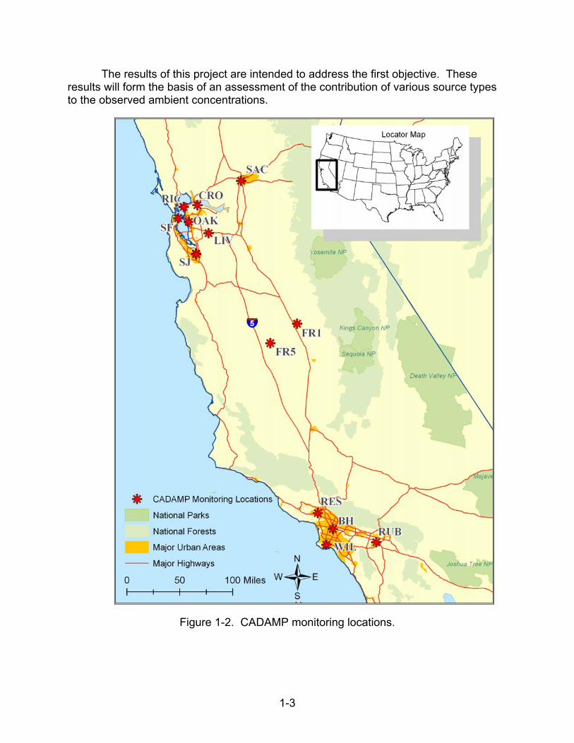
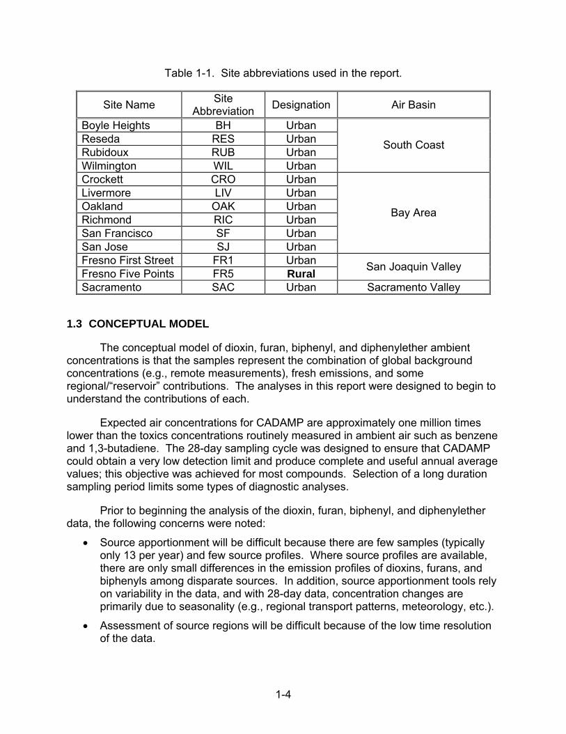
In addition to being located in population centers, CADAMP site locations were chosen based on several factors including, but not limited to, the proximity to potential sources and elevated concentrations of criteria pollutants, toxic air contaminants, and related pollutants. Several of the dioxin monitors were operated in parallel with new monitoring stations that were installed as part of ARB’s Children’s Environmental Health Protection Program. Sites are shown in Figure 1-2 and site abbreviations are listed in Table 1-1.

The specific objectives of CADAMP were to

1. assess airborne concentrations of dioxins, furans, biphenyls, and diphenylethers in populated areas in California potentially impacted by emissions from stationary and mobile sources;

2. provide additional information for the California Children’s Environmental Health Protection Act (Senate Bill SB25, Escutia, 1999) monitoring program by using the same sampling sites.

1-3

The results of this project are intended to address the first objective. These results will form the basis of an assessment of the contribution of various source types to the observed ambient concentrations.

Figure 1-2. CADAMP monitoring locations.

1-4

Table 1-1. Site abbreviations used in the report.

Site Name Site

Abbreviation Designation Air Basin

Boyle Heights BH Urban Reseda RES Urban Rubidoux RUB Urban Wilmington WIL Urban

South Coast

Crockett CRO Urban Livermore LIV Urban Oakland OAK Urban Richmond RIC Urban San Francisco SF Urban San Jose SJ Urban

Bay Area

Fresno First Street FR1 Urban Fresno Five Points FR5 Rural

San Joaquin Valley

Sacramento SAC Urban Sacramento Valley

1.3 CONCEPTUAL MODEL

The conceptual model of dioxin, furan, biphenyl, and diphenylether ambient concentrations is that the samples represent the combination of global background concentrations (e.g., remote measurements), fresh emissions, and some regional/“reservoir” contributions. The analyses in this report were designed to begin to understand the contributions of each.

Expected air concentrations for CADAMP are approximately one million times lower than the toxics concentrations routinely measured in ambient air such as benzene and 1,3-butadiene. The 28-day sampling cycle was designed to ensure that CADAMP could obtain a very low detection limit and produce complete and useful annual average values; this objective was achieved for most compounds. Selection of a long duration sampling period limits some types of diagnostic analyses.

Prior to beginning the analysis of the dioxin, furan, biphenyl, and diphenylether data, the following concerns were noted:

Source apportionment will be difficult because there are few samples (typically only 13 per year) and few source profiles. Where source profiles are available, there are only small differences in the emission profiles of dioxins, furans, and biphenyls among disparate sources. In addition, source apportionment tools rely on variability in the data, and with 28-day data, concentration changes are primarily due to seasonality (e.g., regional transport patterns, meteorology, etc.).

Assessment of source regions will be difficult because of the low time resolution of the data.

1-5

Comparisons between sites and air basins will be somewhat hampered by differences in sampling periods, number of samples, and the total number of samples available at a given site.

Throughout this report, analysis results include a discussion of data limitations and caveats to ensure that results are not over-interpreted. Of particular note, given the strong seasonal patterns in the data, it is important to recognize that correlation between pollutant concentrations and other measures does not imply causation.

1.4 EMISSIONS OF DIOXINS, FURANS, BIPHENYLS, AND DIPHENYLETHERS

Dioxins, furans, biphenyls, and diphenylethers are emitted from a variety of sources and can be re-entrained into the environment after they have deposited to a surface. For example, biphenyls can deposit in water and be re-emitted as vapor when temperatures rise (Baird and Cann, 2005), and all particle bound dioxins, furans, biphenyls, and diphenylethers can be re-suspended as dust. The combination of these mechanisms makes ascribing sources to ambient levels of these compounds difficult.

An important primary source of fresh emissions of dioxins, furans, and biphenyls is combustion, including mobile source emissions, wood burning, and fuel burning. In an urban environment, such as those in which most of the CADAMP monitors are located, mobile sources are expected to be important. Table 1-2 details the vehicle miles traveled (VMT) by county where CADAMP monitoring sites are located. Differences in ambient dioxin, furan, and biphenyl concentrations among sites may be partially explained by the local mobile source activity, so we might expect dioxin, furan, and biphenyl concentrations at Los Angeles County sites to be higher than at other sites. Point sources, including both electrical generating units (EGUs) and other sources such as chemical manufacturing, smelting, etc., are also potentially important sources. Medical waste incineration and backyard barrel burning are two of the largest sources of dioxins, furans, and biphenyls nationally (U.S. Environmental Protection Agency, 2006); however, these sources were regulated in California during CADAMP monitoring and are not expected to contribute to emissions (California Air Resources Board, 2004, 2003).

Table 1-2. VMT by county in 2004 (California Air Resources Board, 2007). Site abbreviations are defined in Table 1-1.

County Sites In County

Air Basin 2004 VMT (thousands

of miles per day)

Los Angeles RES, BH, WIL 232,828 Riverside RUB

South Coast 54,998

Alameda LIV, OAK 35,872 Santa Clara SJ 41,287 Contra Costa CRO, RIC 25,879 San Francisco SF

San Francisco Bay Area

13,184 Sacramento SAC Sacramento Valley 32,244 Fresno FR1, FR5 San Joaquin Valley 20,114

1-6

1.5 OBJECTIVES OF THIS ANALYSIS PROJECT AND ORGANIZATION OF THE REPORT

The primary objective of this report is to begin to better understand the possible sources of dioxins, furans, biphenyls, and diphenylethers in California. Detailed data validation and assessment (Section 2), characterization by spatial and temporal analyses (Section 3), meteorological analyses (Section 4), and source apportionment analyses (Section 5) were conducted. Conclusions and recommendations for further analysis are provided in Section 6. Appendix A contains naming conventions, measured analytes, abbreviations, and toxicity equivalency values. Appendix B provides more details about multiple-linear regression. Appendix C contains Google Earth™ images of each CADAMP site.

2-1

2. DATA ACQUISITION AND PREPARATION

2.1 CADAMP DATA

A database containing monitoring data collected within the CADAMP network was obtained from ARB on October 5, 2007. The database contains measurements of 7 dioxin, 10 furan, 14 biphenyl, and 40 diphenylether congeners at 13 locations in California. This database has been subjected by ARB to a rigorous field and laboratory quality assurance process designed specifically for CADAMP. Selected elements include third-party field flow-rate and system audits at each sampling location, a laboratory systems audit, and performance evaluation samples submitted to both the ARB’s contract laboratory and the EPA NDAMN laboratory. Collocated sampling was included at three CADAMP sites as was parallel sampling at an NDAMN site at Fort Cronkite (San Francisco Bay Area Air Basin).

Data quality measures include the percentage of data below detection and data completeness. The percentage of data below detection demonstrates the ability of an analytical method to characterize ambient concentrations and provides an indication of the usability of the data for subsequent analyses, while data completeness indicates the number of missing samples which is important when calculating valid seasonal and annual averages.

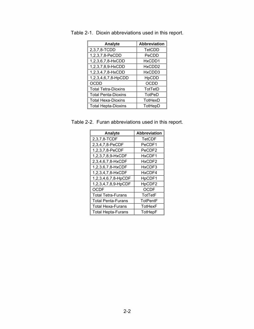
Tables 2-1 through 2-4 contain the naming conventions and abbreviations used in the plots and tables in this report (with additional details in Appendix A). Abbreviations are used to aid in data presentation because most of the compound names are very long and difficult to differentiate. Abbreviations were created to systematically display necessary compound information including the number of chlorine atoms, the compound class, and to facilitate differentiation between congeners. First, the number of chlorine or bromine atoms is indicated by the abbreviation prefix. The compound class is then displayed as “CDD” for –chlorinated dibenzo dioxin, “CDF” for –chlorinated dibenzo furan, “CB” for –chlorinated biphenyl, and “BDE” for –brominated diphenylether. Note that the last letter of the name is enough to identify the compound class (i.e., D for dioxin, F for furan, B for biphenyl, E for diphenylether). Congeners are then differentiated with a numeric suffix; if no suffix is present, then only one congener was measured. For example, TetCDD is a dioxin with four chlorines and no other congeners are measured. PeBDE4 is a diphenylether with five bromines and other congeners are measured.

2-2

Table 2-1. Dioxin abbreviations used in this report.

Analyte Abbreviation

2,3,7,8-TCDD TetCDD 1,2,3,7,8-PeCDD PeCDD 1,2,3,6,7,8-HxCDD HxCDD1 1,2,3,7,8,9-HxCDD HxCDD2 1,2,3,4,7,8-HxCDD HxCDD3 1,2,3,4,6,7,8-HpCDD HpCDD OCDD OCDD Total Tetra-Dioxins TotTetD Total Penta-Dioxins TotPeD Total Hexa-Dioxins TotHexD Total Hepta-Dioxins TotHepD

Table 2-2. Furan abbreviations used in this report.

Analyte Abbreviation

2,3,7,8-TCDF TetCDF 2,3,4,7,8-PeCDF PeCDF1 1,2,3,7,8-PeCDF PeCDF2 1,2,3,7,8,9-HxCDF HxCDF1 2,3,4,6,7,8-HxCDF HxCDF2 1,2,3,6,7,8-HxCDF HxCDF3 1,2,3,4,7,8-HxCDF HxCDF4 1,2,3,4,6,7,8-HpCDF HpCDF1 1,2,3,4,7,8,9-HpCDF HpCDF2 OCDF OCDF Total Tetra-Furans TotTetF Total Penta-Furans TotPentF Total Hexa-Furans TotHexF Total Hepta-Furans TotHepF

2-3

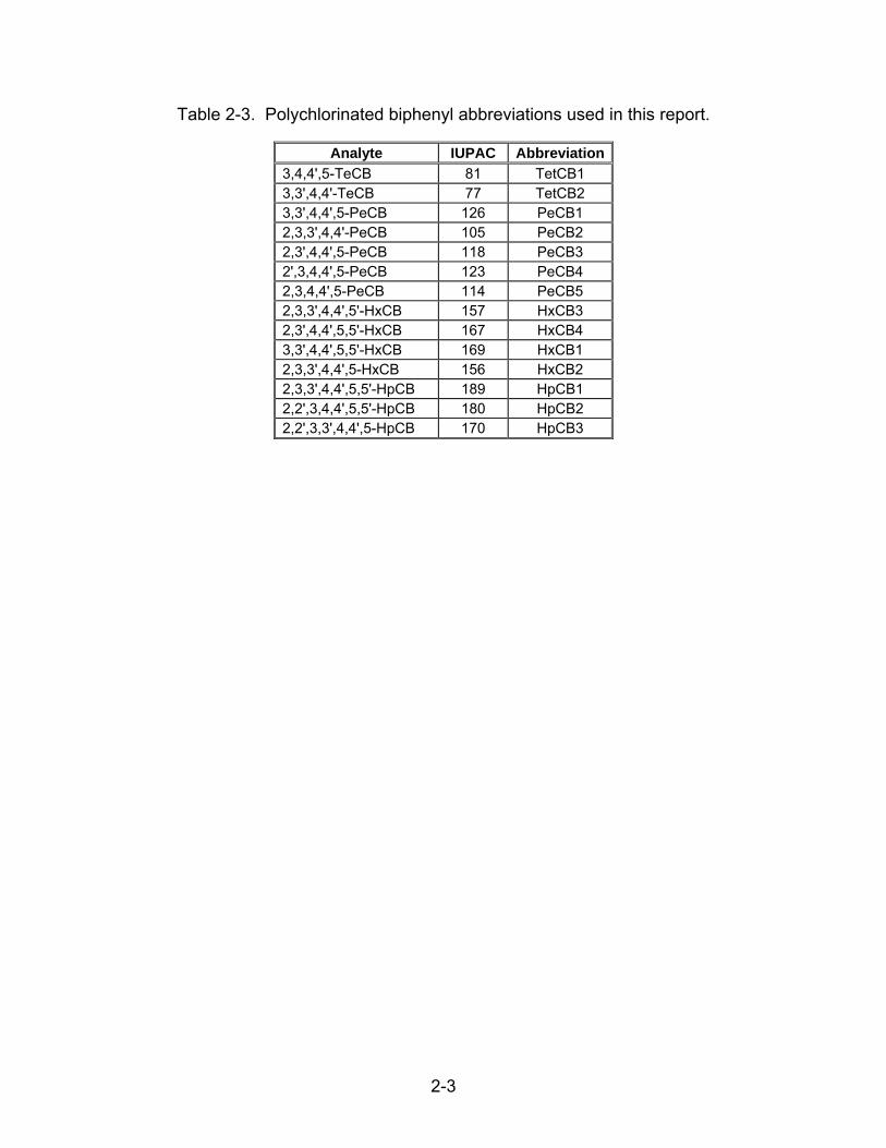
Table 2-3. Polychlorinated biphenyl abbreviations used in this report.

Analyte IUPAC Abbreviation

3,4,4',5-TeCB 81 TetCB1 3,3',4,4'-TeCB 77 TetCB2 3,3',4,4',5-PeCB 126 PeCB1 2,3,3',4,4'-PeCB 105 PeCB2 2,3',4,4',5-PeCB 118 PeCB3 2',3,4,4',5-PeCB 123 PeCB4 2,3,4,4',5-PeCB 114 PeCB5 2,3,3',4,4',5'-HxCB 157 HxCB3 2,3',4,4',5,5'-HxCB 167 HxCB4 3,3',4,4',5,5'-HxCB 169 HxCB1 2,3,3',4,4',5-HxCB 156 HxCB2 2,3,3',4,4',5,5'-HpCB 189 HpCB1 2,2',3,4,4',5,5'-HpCB 180 HpCB2 2,2',3,3',4,4',5-HpCB 170 HpCB3

2-4

Table 2-4. Polybrominated diphenylether abbreviations used in this report.

Analyte IUPAC Abbreviation

2,6-DiBDE 10 DiBDE1 2,4-DiBDE 7 DiBDE2 2,4'-DiBDE 8 DiBDE3 3,4-DiBDE 12 DiBDE4 4,4'-DiBDE 15 DiBDE5 3,4,4'-TriBDE 37 TriBDE1 2,4,4'-TriBDE 28 TriBDE2 2,4,6-TriBDE 30 TriBDE3 2,2',4-TriBDE 17 TriBDE4 2,4',6-TriBDE 32 TriBDE5 3,3',4-TriBDE 35 TriBDE6 3,3',4,4'-TetraBDE 77 TetBDE1 2,2',4,4'-TetraBDE 47 TetBDE2 2,3',4,4'-TetraBDE 66 TetBDE3 2,3',4',6-TetraBDE 71 TetBDE4 2,4,4',6-TetraBDE 75 TetBDE5 2,2',4,5'-TetraBDE 49 TetBDE6 2,2',4,6'-TetraBDE 51 TetBDE7 3,3',4,5'-TetraBDE 79 TetBDE8 2,2',3,4,4'-PentaBDE 85 PeBDE1 2,2',4,4',6-PentaBDE 100 PeBDE2 2,2',4,4',5-PentaBDE 99 PeBDE3 2,3,4,5,6-PentaBDE 116 PeBDE4 2,3',4,4',6-PentaBDE 119 PeBDE5 2,3,3',4,4'-PentaBDE 105 PeBDE6 3,3',4,4',5-PentaBDE 126 PeBDE7 2,2',4,4',5,5'-HexaBDE 153 HxBDE1 2,2',4,4',5,6'-HexaBDE 154 HxBDE2 2,2',3,4,4',5'-HexaBDE 138 HxBDE3 2,2',3,4,4',6'-HexaBDE 140 HxBDE4 2,2',4,4',6,6'-HexaBDE 155 HxBDE5 2,2',3,3',4,4'-HexaBDE 128 HxBDE6 2,2',3,4,4',5',6-HeptaBDE 183 HpBDE1 2,3,3',4,4',5,6-HeptaBDE 190 HpBDE2 2,2',3,4,4',5,6-HeptaBDE 181 HpBDE3 2,2',3,4,4',5,5',6-OctaBDE 203 OBDE 2,2',3,3',4,4',5,6,6'-NonaBDE 207 NonBDE1 2,2',3,3',4,4',5,5',6-NonaBDE 206 NonBDE2 2,2',3,3',4,5,5',6,6'-NonaBDE 208 NonBDE3 2,2',3,3',4,4',5,5',6,6'-DecaBDE 209 DecaBDE

Data completeness was high, spanning a range of 87 to 100 percent completeness by site (Table 2-5). Overall data quality of CADAMP data was excellent. Few dioxin, furan, or biphenyl compounds measured had greater than 50 percent of

2-5

data below detection at a given site (Table 2-6). As a whole, diphenylethers were more frequently below detection than other measured compounds, and 2,4,6-TriBDE3 (TriBDE3) and 3,3’,4-TriBDE (TriBDE6) were always below the limit of detection.

Table 2-5. CADAMP data completeness and sampling timeframe by site. Site abbreviations are defined in Table 1-1.

Site Air Basin Expected Number of Samples

Number of Samples

Percent Completeness

Sampling Date Range

BH 38 38 100 2002-2004 RES 39 34 87 2002-2004 RUB 52 45 87 2002-2005 WIL

South Coast

39 37 95 2002-2004 CRO 38 36 95 2002-2004 LIV 52 52 100 2002-2005 OAK 39 36 92 2002-2004 RIC 39 39 100 2002-2004 SFa 28 28 100 2003-2004 SJ

Bay Area

39 34 87 2002-2004 FR1 18 18 100 2005-6/2006 FR5

San Joaquin Valley 13 12 92 6/2005-6/2006

SAC Sacramento Valley 26 26 100 2003-2004

a SF was a value-added site sponsored by the Bay Area Air Quality Management District.

2-6

Table 2-6. Percentage of data below detection by compound and site. Green indicates 0 to 50 percent below detection, pink indicates >50 percent below detection, and grey indicates the parameter was not measured. Compound abbreviations are defined in Tables 2-1 through 2-4.

Page 1 of 2

South Coast Bay Area San Joaquin SACCompound BH RES RUB WIL CRO LIV OAK RIC SF SJ FR1 FR5 SACTetCDD 2 6 0 3 3 4 5 3 0 0 0 33 0 PeCDD 2 3 0 0 3 0 4 0 0 3 0 0 0 HxCDD1 0 0 0 6 0 0 0 3 0 0 0 0 0 HxCDD2 0 0 0 3 0 0 2 3 0 0 0 0 0 HxCDD3 2 0 0 0 0 0 4 8 11 0 0 0 4 HpCDD 0 0 0 0 0 0 0 0 0 0 0 0 0 OCDD 0 0 0 0 0 0 0 0 0 0 0 0 0 TetCDF 0 0 0 0 0 2 0 3 4 0 0 25 0 PeCDF1 0 0 0 0 3 0 0 3 0 0 0 0 0 PeCDF2 0 3 0 0 3 0 4 0 0 3 8 0 0 HxCDF1 19 23 9 25 28 35 25 24 22 30 15 42 32 HxCDF2 0 0 0 3 3 2 0 0 0 3 4 8 8 HxCDF3 0 0 0 0 3 0 0 0 0 0 0 0 0 HxCDF4 0 3 0 3 0 2 2 5 0 0 4 0 4 HpCDF1 0 0 2 0 0 0 0 0 0 0 0 0 0 HpCDF2 3 0 0 3 3 10 0 5 7 0 4 8 4 OCDF 0 0 0 0 0 0 0 0 0 0 0 0 0 TetCB1 0 3 5 0 8 6 2 3 0 3 8 42 0 TetCB2 0 0 0 0 0 0 0 0 0 0 0 0 0 PeCB1 0 0 5 0 3 0 0 0 0 0 8 58 0 PeCB2 0 0 2 0 0 0 0 0 0 0 0 8 0 PeCB3 0 0 0 0 0 0 0 0 0 0 0 0 0 PeCB4 0 0 5 3 0 2 0 0 0 0 0 58 0 PeCB5 0 3 2 0 3 6 0 0 0 0 0 83 0 HxCB1 32 44 45 36 89 61 46 66 37 52 72 75 24 HxCB2 0 0 2 0 0 0 0 0 4 0 0 8 0 HxCB3 0 0 2 0 0 0 0 0 4 0 0 25 0 HxCB4 0 0 0 0 0 0 0 0 0 0 0 8 0 HpCB1 0 9 5 0 3 4 2 3 0 3 8 33 0 HpCB2 0 0 0 0 0 0 0 0 0 0 0 0 0 HpCB3 0 0 0 0 0 0 0 0 0 0 0 0 0 DiBDE1 91 93 95 85 97 95 91 95 96 100 DiBDE2 0 0 0 0 0 0 0 0 4 0 DiBDE3 0 0 0 0 0 0 0 0 4 0 DiBDE4 26 0 0 0 3 10 4 0 0 17 DiBDE5 0 0 0 0 0 0 0 0 0 0 TriBDE1 0 3 0 0 3 0 4 0 4 42 TriBDE2 0 0 0 0 0 0 0 0 0 8 TriBDE3 100 100 100 100 100 100 100 100 100 100 TriBDE4 0 7 0 0 0 0 0 0 4 33 TriBDE5 47 40 47 69 61 62 48 76 100 92 TriBDE6 100 100 100 100 100 100 100 100 100 100

2-7

Table 2-6. Percentage of data below detection by compound and site. Green indicates 0 to 50 percent below detection, pink indicates >50 percent below detection, and grey indicates the parameter was not measured. Compound abbreviations are defined in Tables 2-1 through 2-4.

Page 2 of 2

South Coast Bay Area San Joaquin SACCompound BH RES RUB WIL CRO LIV OAK RIC SF SJ FR1 FR5 SACTetBDE1 6 13 16 8 28 43 43 29 8 17 TetBDE2 0 0 0 0 0 0 0 0 0 0 TetBDE3 0 0 0 0 0 0 0 0 0 0 TetBDE4 0 0 0 0 8 0 0 0 4 0 TetBDE5 0 0 5 8 0 14 0 0 8 25 TetBDE6 0 0 0 0 0 0 0 0 0 0 TetBDE7 0 0 4 8 TetBDE8 30 15 24 42 PeBDE1 0 0 0 0 0 0 4 0 0 0 PeBDE2 0 0 0 0 0 0 0 0 0 0 PeBDE3 0 0 0 0 0 0 0 0 0 0 PeBDE4 100 90 100 85 100 95 96 95 92 92 PeBDE5 6 7 11 0 6 5 17 0 8 8 PeBDE6 79 63 79 69 100 100 91 100 60 67 PeBDE7 41 57 53 77 78 71 70 52 36 33 HxBDE1 0 0 0 0 0 0 0 0 0 0 HxBDE2 0 0 0 0 0 0 0 0 0 0 HxBDE3 0 3 0 0 0 10 0 0 4 8 HxBDE4 3 0 0 8 3 29 17 0 8 25 HxBDE5 0 3 0 15 0 10 4 0 4 17 HxBDE6 80 85 84 100 HpBDE1 0 3 0 8 0 5 0 0 0 8 HpBDE2 3 7 16 15 19 33 30 10 28 33 HpBDE3 21 33 37 23 42 62 48 29 52 33 OBDE 0 15 8 17 NonBDE1 0 3 0 0 0 0 0 10 4 0 NonBDE2 3 0 0 15 3 5 4 10 4 0 NonBDE3 0 7 0 15 6 14 17 14 12 25 DecaBDE 0 0 0 0 0 0 0 0 0 8 TotHepD 0 0 0 0 0 0 0 0 0 0 0 0 0 TotHepF 0 0 0 0 0 0 0 0 0 0 0 0 0 TotHexD 0 0 0 0 0 0 0 0 0 0 0 0 0 TotHexF 0 0 0 0 0 0 0 0 0 0 0 0 0 TotPeD 0 0 0 0 0 0 0 0 0 0 0 0 0 TotPentF 0 0 0 0 0 0 0 0 0 0 0 0 0 TotTetD 0 0 0 0 0 0 0 0 0 0 0 0 0 TotTetF 0 0 0 0 0 0 0 0 0 0 0 0 0

2-8

2.2 SUPPLEMENTARY DATA SETS

Additional data sets were acquired for comparison to CADAMP, including measurements of dioxins, furans, and biphenyls from EPA’s NDAMN network, parallel measurements of air quality and meteorological data available through EPA’s Air Quality System (AQS), as well as nearby meteorological measurements and derived parameters from surface and upper-air measurements in the National Oceanic and Atmospheric Association (NOAA) monitoring network.

NDAMN data were obtained from Dr. David Cleverly (EPA Office of Research and Development) on October 26, 2007, and contain dioxin, furan, and biphenyl measurements at 9 remote, 21 rural, and 4 urban sites across the United States, including two urban California sites. These data were used for a comparison to CADAMP data and to provide an understanding of the regional and background contribution to ambient concentrations.

Many parallel air quality measurements were available through AQS, including criteria pollutants, volatile organic compounds (VOCs), and speciated particulate measurements. These data were used to assist in source identification.

Meteorological measurements from 2001 through 2006 were obtained from the NOAA National Data Center (NOAA, 2007, 2008) and contain commonly measured parameters (e.g., temperature and relative humidity) as well as derived parameters (e.g., daily maximum mixing height and ventilation index). While all parameters in the database are daily records, some are daily averages, such as average daily wind speed, and some are time-specific, such as morning (12Z) 500-mb heights.1 To match the CADAMP data duration, these daily parameters were averaged over the same time period with a 75 percent completeness requirement. This completeness criterion requires at least 75 percent of expected samples to be present to calculate an average. These data were used to understand the impact of meteorology on concentrations of dioxins, furans, biphenyls, and diphenylethers, and to attempt to remove the strong seasonal patterns that are mostly driven by meteorological conditions in order to better understand source impacts.

NDAMN data have the same 28-day duration as CADAMP data, but only one sample per quarter is collected, while CADAMP data are collected continuously (e.g., 13 28-day measurements per year). Because of the disparity in sampling frequency, annual average concentrations were used to compare NDAMN and CADAMP concentrations. A 75 percent completeness criterion was applied for calculation of valid annual averages.

Supplementary air quality and meteorological measurements are collected at hourly to daily frequency. In order to properly match these data to CADAMP 28-day measurements, the data were first aggregated to daily averages. A 75 percent daily completeness criterion was required if data were collected on a sub-daily sampling schedule. The daily averages were then converted to 28-day averages based on the

1 Table 4-2 provides a complete list of parameters used.

2-9

CADAMP sampling schedule; 75 percent completeness was also required to create valid monthly averages.

2.3 DATA VALIDATION

Raw CADAMP data were validated using collocated data, time series, and fingerprint plots. Collocated data (i.e., a second sample that is collected at the same site during the sampling period with the same equipment type), provide a measure of data quality. Time series analyses are useful in identifying differences in concentrations among compounds or between sites. Fingerprint plots are also useful for comparing among samples and sites.

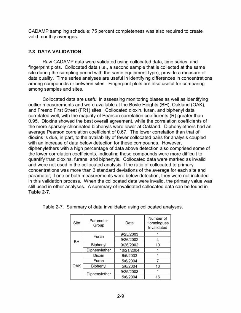
Collocated data are useful in assessing monitoring biases as well as identifying outlier measurements and were available at the Boyle Heights (BH), Oakland (OAK), and Fresno First Street (FR1) sites. Collocated dioxin, furan, and biphenyl data correlated well, with the majority of Pearson correlation coefficients (R) greater than 0.95. Dioxins showed the best overall agreement, while the correlation coefficients of the more sparsely chlorinated biphenyls were lower at Oakland. Diphenylethers had an average Pearson correlation coefficient of 0.67. The lower correlation than that of dioxins is due, in part, to the availability of fewer collocated pairs for analysis coupled with an increase of data below detection for these compounds. However, diphenylethers with a high percentage of data above detection also comprised some of the lower correlation coefficients, indicating these compounds were more difficult to quantify than dioxins, furans, and biphenyls. Collocated data were marked as invalid and were not used in the collocated analysis if the ratio of collocated to primary concentrations was more than 3 standard deviations of the average for each site and parameter; if one or both measurements were below detection, they were not included in this validation process. When the collocated data were invalid, the primary value was still used in other analyses. A summary of invalidated collocated data can be found in Table 2-7.

Table 2-7. Summary of data invalidated using collocated analyses.

Site Parameter

Group Date

Number of Homologues Invalidated

9/25/2003 1 Furan 9/26/2002 4

Biphenyl 9/26/2002 10 BH

Diphenylether 10/21/2004 1 Dioxin 6/5/2003 1 Furan 5/6/2004 7

Biphenyl 5/6/2004 10 9/25/2003 1

OAK

Diphenylether 5/6/2004 16

2-10

A validated data set was prepared that merged the primary and collocated data using the following hierarchy: (1) primary sample always takes precedent if valid; (2) if the primary sample was invalid, missing, or below detection and the collocated sample was valid, the collocated sample was used.

Time-series plots of concentrations of merged data were visually inspected for apparent outliers (measured concentrations more than two times higher than the typical variability in concentration); outliers were marked as suspect and compared with behavior of other homologues. A few large concentration spikes were observed and were typically echoed in all parameters of a group. Due to the 28-day sampling period and agreement between parameters, it was difficult to confidently flag these occurrences as invalid. Outliers were investigated further by comparing compound profiles (i.e., fingerprints) of high concentration events to the average compound profile. Differences in profiles for high concentration events may indicate the presence of an additional source causing the concentration spike; however, the relative ratios of compounds were consistent between high and median profiles and did not indicate any additional sources. A spike in 1,2,3,4,7,8,9-HpCDF (HpCDF2) nearly five times the typical maximum concentration was observed at Crockett on February 14, 2002, which was not apparent in other furan homologues. Fingerprint plots showed an atypical ratio of HpCDF2 to other furan compounds; however, all other furan compounds were similar to the average fingerprint profile. The outlier value was 999, which was likely meant to be “-999”, an invalid data code. This observation coupled with the fact that 1,2,3,4,7,8,9-HpCDF (HpCDF2) was the only furan in that sample to show a marked difference in behavior led to invalidation of the data point2. Sufficient evidence could not be found to invalidate other high concentration events so they were marked as suspect and tracked in data aggregates (e.g., seasonal and annual averages). Whenever possible, median concentrations were used instead of means in subsequent analyses to reduce biases by high concentration values.

Data validation of CADAMP dioxin, furan, and biphenyl data showed a dataset of good accuracy (i.e., collocated agreement), and data quality (i.e., few invalid or suspect samples) that successfully measured very low concentrations (i.e., most data above detection). Diphenylether data showed less accuracy (i.e., collocated disagreement) as well as more data below detection, more than 50 percent of data below detection at all sites for 6 out of 40 measured compounds.

2.4 PREPARATION OF DATA AGGREGATES

Seasonal and annual aggregates were prepared from the CADAMP 28-day data. Because of the long sampling period, a “rounding” methodology was developed to create representative seasonal and annual averages. For example, some samples began December 20, 2001. Eleven of the sampling days represent December 2001, while 17 of the sampling days represent January 2002. Because this sample is more 2 Subsequent to delivery of this report, ARB checked this value and determined it to be a valid concentration of 999 fg/m3. Analyses were not updated.

2-11

representative of January 2002, the month and year were rounded, as was any sample with greater than 50 percent of the sampling period attributed to the next month.

Completeness requirements for seasonal and annual aggregates were 2 of 3 samples and 3 of 4 quarters, respectively. Suspect data were included in data aggregates and the number of suspect samples included in the aggregate was tabulated; all invalid data were excluded from data aggregates. The annual average was defined as spanning a calendar year. For some site-compound combinations, while a year or more of data was collected, the data did not meet our completeness criteria for an annual average over a calendar year.

TEQ values were calculated for total dioxins (TEQD), furans (TEQF), and biphenyls (TEQB); dioxins plus furans (TEQD/F); and total TEQ (TEQTOT) where TEQTOT is the sum of all dioxin, furan, and biphenyl compounds. These values are calculated as the sum of the individual compound World Health Organization 97 (WHO-97) TEQs and represent the total toxicity of the respective groups. WHO-97 TEFs were not available for 2,2’,3,4,4’,5,5’-HpCB (HpCB2) and 2,2’3,3’,4,4’,5-HpCB (HpCB3), so the WHO-94 TEFs were used. In order to create a valid measure of toxicity, a consistent suite of measured compounds within a group was required to be present; for example, all 10 furan compounds measured were required to be present to calculate TEQF. Samples were considered to be present if they were below detection; missing compounds were mainly due to data that had been previously invalidated. TEQ values were calculated using both zero and MDL/2 for values below detection. For brevity, only results using zero substitutions are included in the report.

3-1

3. CHARACTERIZATION OF DIOXINS, FURANS, BIPHENYLS, AND DIPHENYLETHERS

3.1 TECHNICAL APPROACH

Building on the existing summary analyses prepared by ARB, additional analyses were performed to further understand the spatial and temporal patterns and variability in the data. The following tools for analyses are discussed in this section:

Investigation of scatter plots (and correlations) among pollutants.

Analysis of variance (ANOVA) of sites grouped by air basin to examine between-site and within-site variance as well as by all air basins of interest to examine variations across air basins. ANOVA tables were constructed for each parameter by site and air basin. The tables indicate if a variable of interest (e.g., species concentration) is statistically significantly dependent on a given grouping (e.g., site location). ANOVA does this by comparing the variability between groups with the variability within a group. If the p-value reported in the ANOVA table is less than or equal to 0.05, the variable is considered statistically significantly dependent on the grouping at a 95 percent confidence level.

Comparison of box whisker plots of pollutants across sites to examine statistically significant differences in concentrations as well as differences in distributions across sites. For example, a notched box plot can show if the median concentration at a site is statistically significantly different than at other sites. Notched box plots (Figures 3-1 and 3-2) are particularly efficient for examining multiple pollutants because they are easier to visually assess than tables.

Spatial principal component analysis (PCA), including multiple sites in one data set, to see how sites group together. Sites that group together likely have similar source impacts.

Analyses were performed for compound groupings and individual compounds at monthly, quarterly, and annual average levels. Summary tables and graphs provide both concentrations and TEQs where appropriate. For presentation of results, data were grouped by air basin: South Coast Air Basin; San Francisco Bay Air Basin; Sacramento Valley Air Basin; and San Joaquin Valley Air Basin.

The relationship of the compound groups and key species to other pollutants such as ozone, particulate matter (PM2.5), carbon monoxide (CO), oxides of nitrogen (NOx), and air toxics (as available) was also investigated using scatter plots/correlation coefficients. A strong correlation between a measured compound/compound group and a pollutant that shows a significant mobile source emission influence, for example, implies that the measured compound/compound group may also be influenced by mobile sources. Because the 28-day sampling may weaken any observed temporal relationship (and the number of samples at some sites may limit statistical analyses), seasonal and monthly averages were also plotted and compared qualitatively to look for similar trends across pollutants.

3-2

The CADAMP data were put into national perspective by comparing the measured concentrations in California’s program with those at other sites in California and the United States from the mostly rural NDAMN program and current literature. Estimates of the percent of each pollutant likely due to background concentrations using reported values of national rural background and remote background concentrations were made.

25th percentile

75th percentile

0

100

200

300

Mea

sure

Outliers

Notcharoundmedian

Median

95 % C.I.

95 % C.I.

Whisker

25th percentile

75th percentile

0

100

200

300

Mea

sure

Outliers

Notcharoundmedian

Median

95 % C.I.

95 % C.I.

Whisker

Figure 3-1. Interpretation of notched box plots produced by SYSTAT. Boxes show the 25th to 75th percentiles (interquartile range, IQR), whiskers extend to 1.5*IQR, and concentrations beyond the whiskers are designated with star symbols. Concentrations beyond 3*IQR are designated with open circles. The median and 95 percent confidence interval (C.I.) are shown as a notch.

3-3

0

10

20

30

40

50M

easu

re

75th Percentile

25th Percentile

95th %Confidence

Interval

0

10

20

30

40

50M

easu

re

75th Percentile

25th Percentile

95th %Confidence

Interval

Figure 3-2. Interpretation of a special case of notched box plots produced by Systat.

It is sometimes possible for the 95 percent confidence interval to be outside the interquartile range. In Figure 3-2, the 25th percentile is larger than the lower 95 percent confidence interval. When this occurs, all statistical representations are the same as the typical notched box plot, but the plot takes on the folded appearance apparent at the bottom of the box in Figure 3-2.

3.2 SUMMARY OF CONCENTRATION RANGES

The summary of concentration ranges provides an overview of dioxin, furan, biphenyl, and diphenylether concentrations observed in California from 2003-2006.

3.2.1 Concentration Ranges within the CADAMP Network

A summary of toxic equivalency quotient (TEQ) concentration ranges measured in the CADAMP network can be found in Table 3-1; more spatially and temporally detailed statistics are discussed further in this section. TEQ values were calculated for total dioxins (TEQD), furans (TEQF), and biphenyls (TEQB); dioxins plus furans (TEQD/F); and total TEQ (TEQTOT) where TEQTOT is the sum of all dioxin, furan, and biphenyl compounds. Statistics were calculated using zero for data below detection. While some compounds (e.g., OCDD, OCDF, and 2,2’,3,4,4’,5,5’-HpCB [HpCB2]) were always

3-4

above detection, the minimum TEQ values reported in Table 3-1 likely consist of multiple compounds below detection and, therefore, may be regarded as a lower estimate.

Table 3-1. TEQ concentration ranges measured in the CADAMP network using all available data (2003-2006). TEQ abbreviations are defined in the text.

Group Minimum Maximum Mean Standard Deviation

Median

TEQD 1.7 170 14 15 9.4 TEQF 0.80 86 9.5 9.3 6.4 TEQD/F 2.6 190 24 22 16 TEQB 0.060 22 5.6 3.8 4.8 TEQTOT 2.8 190 29 22 24

TEF values have not been defined for diphenylethers, so aggregation to TEQ cannot be performed. A summary of the average and range of diphenylether compound concentrations is shown in Table 3-2.

3.2.2 Comparison to NDAMN

To put the CADAMP data into a national perspective, concentration ranges of CADAMP data were compared with concentration ranges of NDAMN data. The NDAMN network contains mostly rural and remote sites and is expected to have lower concentrations than the CADAMP network, which mainly consists of urban sites. Annual average concentrations were used for inter-comparison because of discrepancies in sampling frequency between networks; NDAMN samples were collected once per quarter, while CADAMP samples were collected continuously. A 75 percent annual completeness criterion was required to calculate annual averages. Additionally, NDAMN sampled only 7 of the 14 biphenyl compounds measured by CADAMP; other measured compound groups are comparable. CADAMP biphenyl TEQs used in these analyses were recalculated to include only those 7 biphenyls to facilitate a valid comparison.

Table 3-3 contains a list of NDAMN monitoring locations along with monitor type designations; NDAMN monitors located in California are in bold text. There are no formally accepted definitions of the terms urban, rural, and remote: usually urban and rural make up a contrasting pair. The most important distinction between all three lies in population density (and in the present context, local emissions density) but there are no firmly established limits. In very rough terms, rural implies a population density between 10 and 100 people per square km. Urban and remote are above and below these densities, respectively. These three terms are thus undefined but reasonably well understood.

3-5

Table 3-2. Average and range of diphenylether compound concentrations using all available data (2004-2006). Abbreviations are defined in Tables 2-1 through 2-4.

Parameter Average

Concentration (fg/m3) Minimum Concentration

(fg/m3) Maximum Concentration

(fg/m3) DiBDE1 0.20 * 9.3 DiBDE2 140 * 1100 DiBDE3 380 39 3900 DiBDE4 250 * 3400 DiBDE5 690 43 3700 TriBDE1 150 * 1100 TriBDE2 2800 * 19000 TriBDE3a * * * TriBDE4 1500 * 7200 TriBDE5 22 * 890 TriBDE6 a * * * TetBDE1 36 * 230 TetBDE2 53000 2200 1600000 TetBDE3 1900 130 42000 TetBDE4 340 * 4900 TetBDE5 150 * 3100 TetBDE6 2200 170 36000 TetBDE7 180 * 1200 TetBDE8 70 * 400 PeBDE1 1800 * 66000 PeBDE2 9900 350 370000 PeBDE3 47000 1400 2100000 PeBDE4 4.1 * 140 PeBDE5 170 * 4600 PeBDE6 5.2 * 170 PeBDE7 15 * 350 HxBDE1 3000 8.6 87000 HxBDE2 3100 63 100000 HxBDE3 290 * 5500 HxBDE4 130 * 2900 HxBDE5 290 * 12000 HxBDE6 5.0 * 100 HpBDE1 950 * 23000 HpBDE2 87 * 2000 HpBDE3 17 * 100 OBDE 290 * 1500 NonBDE1 1000 * 7500 NonBDE2 920 * 9200 NonBDE3 700 * 6100 DecaBDE 19000 * 95000

a Indicates 100 percent of data below the limit of detection. * Indicates value is below the limit of detection.

3-6

Table 3-3. Summary of NDAMN monitoring locations used in analyses with monitor type designations.

Site State Type

Fort Cronkhitea CA Urban Rancho Seco CA Urban Beltsville MD Urban Newport OR Urban Craig AK Rural Arkadelphia AR Rural Everglades FL Rural Quincy FL Rural McNay IA Rural Dixon Springs IL Rural Monmouth IL Rural Fond Du Lac MN Rural Bay St. Louis MS Rural Clinton Crops NC Rural North Platte NE Rural Jasper NY Rural Caldwell OH Rural Oxford OH Rural Bixby OK Rural Lake Keystone OK Rural Hyslop Farms OR Rural Penn Nursery PA Rural Padre Island TX Rural Bennington VT Rural Lake Dubay WI Rural Trapper Creek AK Remote Chiricahua AZ Remote Grand Canyon AZ Remote Craters Moon ID Remote Lake Scott KS Remote T. Roosevelt N.P. ND Remote Goodwell OK Remote Big Bend TX Remote Ozette Lake WA Remote

a The Fort Cronkhite NDAMN site is classified as an urban site; however, a Google Earth investigation showed that it is not representative of an urban location. Fort Cronkite (alternative spelling) data were not included in statistical summaries of urban concentrations; this site was treated separately in this report.

3-7

When all NDAMN sites were included, CADAMP TEQ ranges for dioxins, furans, and biphenyls were higher than NDAMN TEQ ranges (Figure 3-3). The 10th to 90th percentiles of all groups overlapped, but the 25th to 75th percentile ranges did not. Twenty-one of the NDAMN sites are considered rural and nine are considered remote; lower concentrations are expected at these sites compared with those at urban sites which typically are nearer primary sources.

Fresno Five Points (FR5), the CADAMP rural site, is separated from urban CADAMP sites in Figure 3-3 so it can be compared directly to NDAMN data. The FR5 data point consists of a single annual average of 12, 2005-2006 measurements. Dioxin, biphenyl, and furan TEQ values at FR5 are within the interquartile range of NDAMN TEQ values.

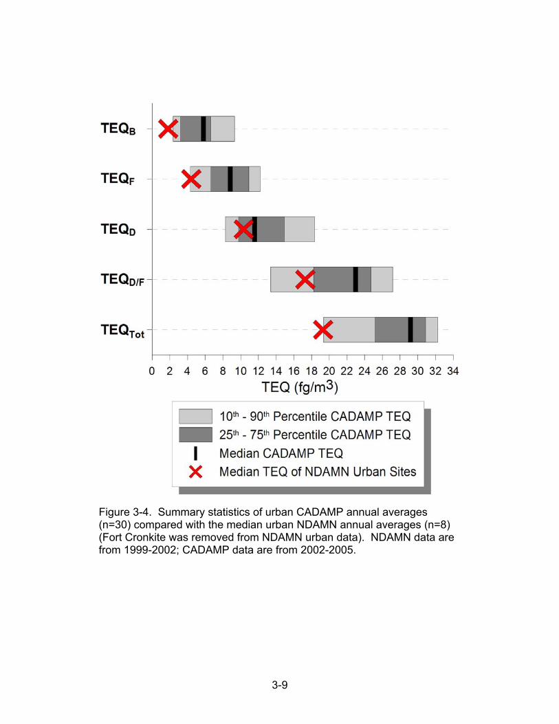
Rural and remote NDAMN sites were then removed to compare CADAMP concentrations to urban NDAMN concentrations. The Fort Cronkite NDAMN site is classified as an urban site; however, a Google Earth investigation showed that it is not representative of an urban location so it was removed from statistical calculations shown in Figure 3-4. Not enough valid annual averages were available to calculate percentiles when only urban NDAMN sites were considered, so only the median NDAMN concentration is included. Figure 3-4 compares the median urban NDAMN concentrations to CADAMP concentration ranges. NDAMN median urban concentrations are less than the 25th percentile of CADAMP concentrations, with the exception of dioxin (TEQD), which is between the 25th and 50th percentile CADAMP concentration.

CADAMP concentration ranges were also compared with the two California NDAMN sites: Rancho Seco and Fort Cronkite (Figure 3-5). Both California NDAMN sites are designated as urban. The median Fort Cronkite TEQs were well below the CADAMP TEQ ranges. Fort Cronkite is located in a relatively isolated coastal area of Marin County which likely explains the low concentrations observed there. The median Rancho Seco TEQs were closer to CADAMP values, but were below the median of CADAMP concentrations for all groups except the dioxins, which were above the 75th percentile CADAMP TEQ. Rancho Seco is located in the outskirts of Sacramento County and is expected to have an urban influence, but is not in the center of an urban area, as are many of the CADAMP sites. Other than the dioxins, the relationship of California concentrations observed in Figure 3-5 is in line with our expectations based on the NDAMN and CADAMP site locations.

In the three comparisons, NDAMN TEQB values were lower than CADAMP TEQB values, typically below the 25th percentile (Figures 3-3 through 3-5). NDAMN TEQF values were lower but had more overlap with CADAMP TEQF values (Figures 3-3 and 3-4). NDAMN TEQD values were lower than CADAMP TEQD values at rural and remote sites (Figure 3-3), however urban NDAMN TEQD values were within the interquartile range of CADAMP values (Figure 3-4) and some urban NDAMN sites were above the 75th percentile CADAMP TEQD value. Though monitoring and temporal differences may affect measured concentrations, the relative TEQ values from both monitoring networks fit our conceptual model of expected concentrations based on site location, providing confidence in this comparison.

3-8

Figure 3-3. CADAMP annual averages (n=30) compared with all NDAMN annual averages (9 remote, 21 rural, and 4 urban sites [n=98]). FR5, the CADAMP rural site, is displayed separately from urban CADAMP data. NDAMN data are from 1999-2002, CADAMP data are from 2002-2005, and CADAMP rural data are a single average of 2005 and 2006 data.

3-9

Figure 3-4. Summary statistics of urban CADAMP annual averages (n=30) compared with the median urban NDAMN annual averages (n=8) (Fort Cronkite was removed from NDAMN urban data). NDAMN data are from 1999-2002; CADAMP data are from 2002-2005.

3-10

Figure 3-5. Summary statistics of urban CADAMP annual averages (n=30) compared with the median annual average at two California NDAMN sites: Rancho Seco and Fort Cronkite. NDAMN data are from 1999-2002; CADAMP data are from 2002-2005.

3-11

3.2.3 Comparison of CADAMP and NDAMN Fingerprints

To look for differences in sources and source strength in rural and remote areas compared with the CADAMP network, fingerprint plots were created using normalized concentrations of dioxins and furans. The normalized concentration is the relative contribution to the total fingerprint, calculated by dividing each species median concentration by the sum of the median concentrations of each species type. This is done to examine differences in the relative contribution to the total fingerprint that may not be as noticeable if absolute concentrations were used due to large differences in median concentrations for urban, rural, and remote sites. Additionally, the differences in CADAMP and NDAMN data are consistent across groups and these effects will be minimized by normalization. Rural and remote fingerprints are also shown as a percent of urban concentrations. FR5, the CADAMP rural site, was not included in analyses so that CADAMP data would represent urban concentrations only.

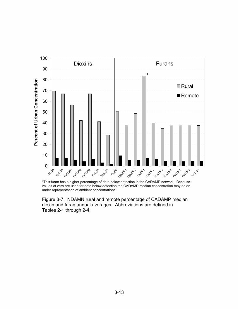
Figures 3-6 and 3-7 show that furans have a relatively constant percentage of urban concentrations across all species while the dioxins have a decreasing percent of urban concentration with a decrease in number of chlorine atoms. The dioxin profile indicates that rural and remote dioxins are aged, that is, these areas do not have as many sources as the California urban areas. The fact that furans show a relatively consistent percentage across compounds within this group may indicate that they do not weather as quickly as dioxins, or that there are more furan sources in remote and rural areas.

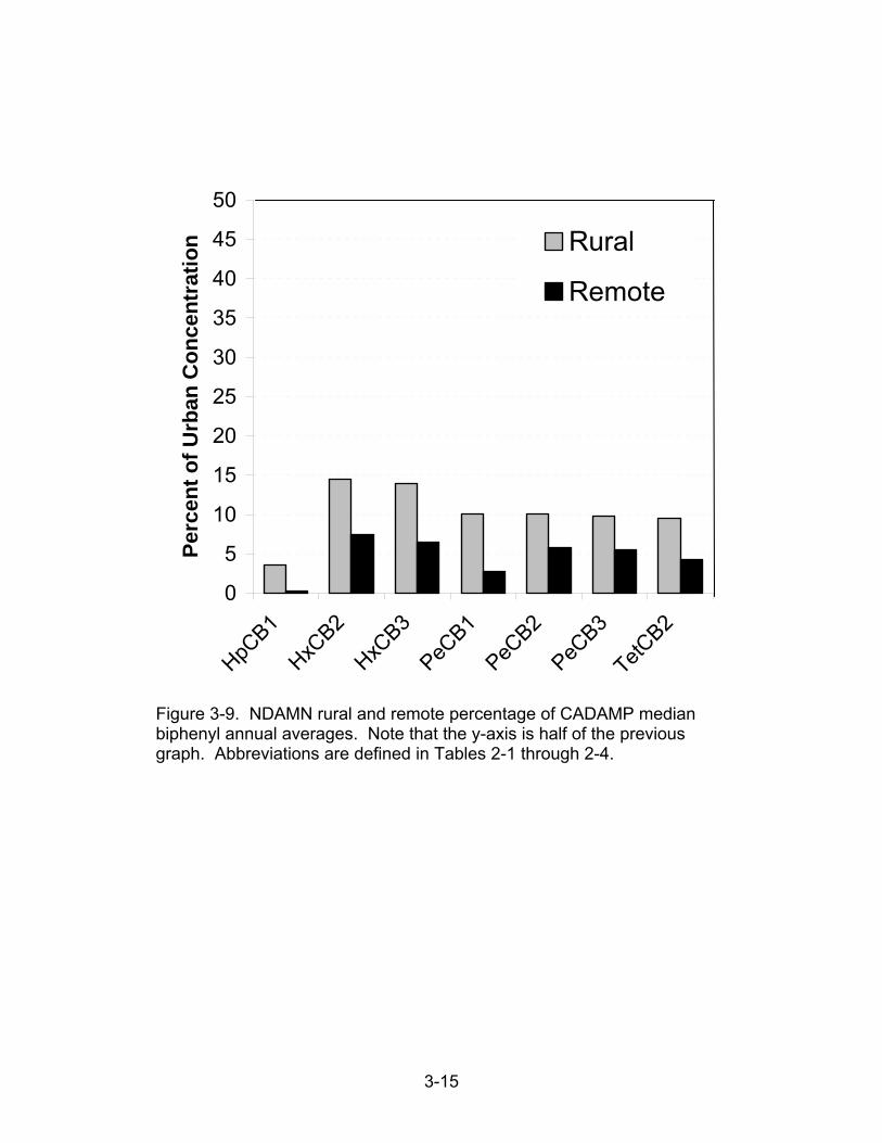
The biphenyl percentage of urban concentration (Figures 3-8 and 3-9) is similar to the furan profile—the percentage of urban concentration is relatively consistent across compounds within a group. Urban biphenyl concentrations measured in the CADAMP network are much higher than those measured in rural and remote areas by the NDAMN network. This indicates that biphenyl species are not as long-lived as dioxin and furan compounds. A numerical summary of the NDAMN percentage of urban concentration is shown in Table 3-4.

A literature review was conducted to compare data from other areas and historical data with CADAMP concentrations (Lohmann and Jones, 1998). However, similar time periods and methods were not available, and the concentration ranges reported in the literature were an order of magnitude or more larger than CADAMP concentrations. It is likely that analysis methods, sampling periods, and reporting differences influence this discrepancy.

3-12

(a)

0.0001

0.001

0.01

0.1

1

OCDD HpCDD HxCDD1 HxCDD2 HxCDD3 PeCDD TetCDD

No

rmal

ized

Co

nce

ntr

ati

on

CADAMP (Urban)

NDAMN Rural

NDAMN Remote

(b)

0.0001

0.001

0.01

0.1

1

OCDFHpC

DF1HpC

DF2HxC

DF1HxC

DF2HxC

DF3HxC

DF4PeC

DF1PeC

DF2

TetCDF

No

rmal

ized

Co

nce

ntr

atio

n

CADAMP (Urban)

NDAMN Rural

NDAMN Remote

Figure 3-6. Normalized median fingerprint plots for (a) dioxins and (b) furans. Data were normalized to the sum of median concentration by group (so bars represent the relative contribution of each species). Figures are displayed on a log scale. Abbreviations are defined in Tables 2-1 through 2-4.

3-13

0

10

20

30

40

50

60

70

80

90

100

OCDD

HpCDD

HxCDD1

HxCDD2

HxCDD3

PeCDD

TetCDD

OCDF

HpCDF1

HpCDF2

HxCDF1

HxCDF2

HxCDF3

HxCDF4

PeCDF1

PeCDF2

TetCDF

Per

cen

t o

f U

rban

Co

nce

ntr

ati

on

Rural

Remote

Dioxins Furans

*

*This furan has a higher percentage of data below detection in the CADAMP network. Because values of zero are used for data below detection the CADAMP median concentration may be an under representation of ambient concentrations.

Figure 3-7. NDAMN rural and remote percentage of CADAMP median dioxin and furan annual averages. Abbreviations are defined in Tables 2-1 through 2-4.

3-14

0.00001

0.0001

0.001

0.01

0.1

1

HpCB1 HxCB2 HxCB3 PeCB1 PeCB2 PeCB3 TetCB2

No

rmal

ized

Co

nce

ntr

atio

n

CADAMP (Urban)

NDAMN Rural

NDAMN Remote

Figure 3-8. Normalized median fingerprint plots for biphenyls. Data were normalized to the sum of median concentration by group. Figures are displayed on a log scale. Abbreviations are defined in Tables 2-1 through 2-4.

3-15

0

5

10

15

20

25

30

35

40

45

50

HpCB1

HxCB2

HxCB3

PeCB1

PeCB2

PeCB3

TetCB2

Per

cen

t o

f U

rban

Co

nce

ntr

atio

n Rural

Remote

Figure 3-9. NDAMN rural and remote percentage of CADAMP median biphenyl annual averages. Note that the y-axis is half of the previous graph. Abbreviations are defined in Tables 2-1 through 2-4.

3-16

Table 3-4. NDAMN rural and remote percentage of CADAMP urban concentrations. Abbreviations are defined in Tables 2-1 through 2-4.

Compound

NDAMN Rural Median Annual Average

Percentage of CADAMP Concentration

NDAMN Remote Median Annual Average

Percentage of CADAMP Concentration

OCDD 69.8 7.3 HpCDD 66.9 7.4 HxCDD1 56.4 5.6 HxCDD2 42.2 4.1 HxCDD3 67.1 6.4 PeCDD 41.2 3.1 TetCDD 28.9 1.9 OCDF 50.5 9.5 HpCDF1 38.1 5.5 HpCDF2 48.8 5.2 HxCDF1 83.4 7.2 HxCDF2 40.1 6.0 HxCDF3 34.9 4.5 HxCDF4 37.4 4.5 PeCDF1 37.3 4.0 PeCDF2 37.9 4.6 TetCDF 37.7 4.5 HpCB1 3.6 0.3 HxCB2 14.4 7.4 HxCB3 13.9 6.5 PeCB1 10.1 2.8 PeCB2 10.1 5.7 PeCB3 9.8 5.5 TetCB2 9.5 4.3

3.3 CORRELATIONS AMONG COMPOUNDS

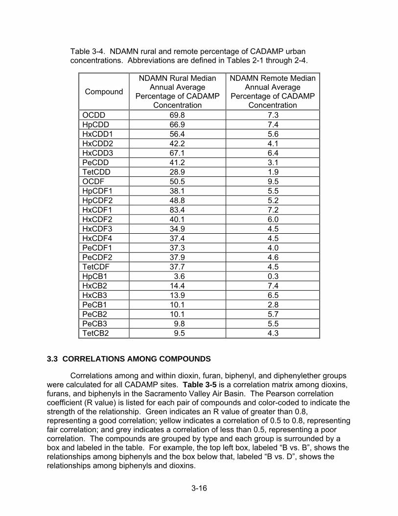
Correlations among and within dioxin, furan, biphenyl, and diphenylether groups were calculated for all CADAMP sites. Table 3-5 is a correlation matrix among dioxins, furans, and biphenyls in the Sacramento Valley Air Basin. The Pearson correlation coefficient (R value) is listed for each pair of compounds and color-coded to indicate the strength of the relationship. Green indicates an R value of greater than 0.8, representing a good correlation; yellow indicates a correlation of 0.5 to 0.8, representing fair correlation; and grey indicates a correlation of less than 0.5, representing a poor correlation. The compounds are grouped by type and each group is surrounded by a box and labeled in the table. For example, the top left box, labeled “B vs. B”, shows the relationships among biphenyls and the box below that, labeled “B vs. D”, shows the relationships among biphenyls and dioxins.

3-17

Table 3-5. Sample correlation matrix among dioxin (D), furan (F), and biphenyl (B) compounds at Sacramento. Green indicates an R value above 0.8, yellow indicates an R value from 0.5 – 0.8, and grey indicates an R value below 0.5. Abbreviations are defined in Tables 2-1 through 2-4.

TE

TC

B1

TE

TC

B2

PE

CB

1

PE

CB

2

PE

CB

3

PE

CB

4

PE

CB

5

HX

CB

1

HX

CB

2

HX

CB

3

HX

CB

4

HP

CB

1

HP

CB

2

HP

CB

3

OC

DD

HP

CD

D

HX

CD

D1

HX

CD

D2

HX

CD

D3

PE

CD

D

TE

TC

DD

OC

DF

HP

CD

F1

HP

CD

F2

HX

CD

F1

HX

CD

F2

HX

CD

F3

HX

CD

F4

PE

CD

F1

PE

CD

F2

TE

TC

DF

TETCB1 1.0

TETCB2 0.8 1.0

PECB1 0.6 0.8 1.0

PECB2 0.8 1.0 0.9 1.0

PECB3 0.8 1.0 0.9 1.0 1.0

PECB4 0.8 1.0 0.9 1.0 1.0 1.0

PECB5 0.8 1.0 0.9 1.0 1.0 1.0 1.0

HXCB1 0.1 0.1 0.3 0.0 0.0 0.1 0.0 1.0

HXCB2 0.8 1.0 0.9 1.0 1.0 1.0 1.0 0.0 1.0

HXCB3 0.8 1.0 0.9 1.0 1.0 1.0 1.0 0.1 1.0 1.0

HXCB4 0.7 1.0 0.9 1.0 1.0 1.0 1.0 0.0 1.0 1.0 1.0

HPCB1 0.7 0.8 0.8 0.8 0.8 0.8 0.8 0.4 0.8 0.9 0.8 1.0

HPCB2 0.8 1.0 0.9 1.0 1.0 1.0 1.0 0.0 1.0 1.0 1.0 0.9 1.0

HPCB3 0.8 0.9 0.9 1.0 1.0 1.0 1.0 0.1 1.0 1.0 1.0 0.9 1.0 1.0

OCDD 0.2 0.4 0.1 0.3 0.3 0.3 0.3 0.5 0.3 0.2 0.3 0.1 0.2 0.2 1.0

HPCDD 0.2 0.4 0.1 0.3 0.3 0.4 0.3 0.6 0.3 0.2 0.3 0.1 0.2 0.2 1.0 1.0

HXCDD1 0.1 0.3 0.0 0.3 0.3 0.3 0.3 0.7 0.2 0.2 0.2 0.2 0.2 0.1 0.9 1.0 1.0

HXCDD2 0.2 0.4 0.1 0.3 0.3 0.3 0.3 0.7 0.3 0.2 0.3 0.1 0.2 0.2 0.9 1.0 1.0 1.0

HXCDD3 0.2 0.4 0.0 0.3 0.3 0.3 0.3 0.6 0.2 0.2 0.2 0.1 0.2 0.2 1.0 1.0 1.0 1.0 1.0

PECDD 0.0 0.2 0.1 0.2 0.2 0.2 0.2 0.7 0.1 0.1 0.1 0.3 0.1 0.0 0.9 1.0 1.0 1.0 1.0 1.0

TETCDD 0.1 0.0 0.3 0.0 0.0 0.0 0.0 0.8 0.1 0.1 0.1 0.5 0.1 0.2 0.7 0.8 0.9 0.9 0.8 0.9 1.0

OCDF 0.2 0.3 0.0 0.3 0.3 0.3 0.3 0.9 0.2 0.2 0.2 0.3 0.2 0.1 0.7 0.8 0.9 0.9 0.8 0.8 0.9 1.0

HPCDF1 0.2 0.3 0.1 0.2 0.2 0.3 0.2 0.9 0.2 0.1 0.2 0.3 0.1 0.1 0.6 0.7 0.7 0.7 0.7 0.7 0.8 1.0 1.0

HPCDF2 0.3 0.4 0.0 0.3 0.3 0.4 0.3 0.9 0.3 0.2 0.3 0.2 0.2 0.2 0.7 0.8 0.8 0.8 0.8 0.8 0.8 1.0 1.0 1.0

HXCDF1 0.1 0.3 0.1 0.2 0.2 0.2 0.2 0.9 0.1 0.1 0.2 0.3 0.1 0.1 0.7 0.8 0.9 0.9 0.8 0.9 0.9 0.9 0.9 0.9 1.0

HXCDF2 0.3 0.4 0.0 0.3 0.3 0.3 0.3 0.9 0.2 0.2 0.2 0.2 0.2 0.2 0.6 0.7 0.7 0.7 0.7 0.7 0.8 1.0 1.0 1.0 0.9 1.0

HXCDF3 0.2 0.3 0.0 0.3 0.3 0.3 0.3 0.9 0.2 0.2 0.2 0.3 0.2 0.1 0.6 0.7 0.8 0.8 0.7 0.8 0.8 1.0 1.0 1.0 0.9 1.0 1.0

HXCDF4 0.2 0.3 0.0 0.3 0.3 0.3 0.3 0.9 0.2 0.2 0.2 0.3 0.2 0.1 0.6 0.7 0.8 0.8 0.7 0.8 0.8 1.0 1.0 1.0 0.9 1.0 1.0 1.0

PECDF1 0.4 0.4 0.1 0.4 0.4 0.4 0.4 0.9 0.3 0.3 0.3 0.1 0.3 0.2 0.5 0.6 0.6 0.7 0.6 0.6 0.7 0.9 0.9 0.9 0.8 1.0 0.9 0.9 1.0

PECDF2 0.2 0.3 0.0 0.3 0.3 0.3 0.3 0.9 0.2 0.2 0.2 0.3 0.2 0.1 0.7 0.8 0.9 0.9 0.8 0.9 0.9 1.0 1.0 1.0 0.9 1.0 1.0 1.0 0.9 1.0

TETCDF 0.0 0.2 0.1 0.2 0.2 0.2 0.2 0.8 0.1 0.1 0.1 0.3 0.1 0.0 0.8 0.9 0.9 0.9 0.9 0.9 0.9 0.9 0.8 0.9 0.9 0.8 0.9 0.8 0.7 0.9 1.0

B vs. B

D vs. D

F vs. F

B vs. D

B vs. F D vs. F

3-18

The correlations in Table 3-5 are typical of those observed at all sites. There is good correlation within each group (e.g., F vs. F) with the exception of 3,3’4,4’5,5’-HxCB (HxCB1) in the biphenyl group. A high percentage of 3,3’4,4’5,5’-HxCB (HxCB1) data was below detection at most sites (40-75 percent) causing the low correlation with all other parameters. However, only 24 percent of HxCB1 data was below detection at Sacramento, and a fair to good correlation with dioxins and furans is shown which is not typical of other data. Investigation of the time series of this species at Sacramento showed a seasonal pattern that was opposite that of other biphenyls and very similar to that of dioxins and furans. Comparison between parameter types shows fair to good correlations between dioxins and furans, and poor correlations between biphenyls and either dioxins or furans.

Diphenylethers were too numerous to succinctly include in Table 3-5. Overall, correlations among diphenylethers were inconsistent. The best correlations within the diphenylether group were between the highest chlorinated (Cl = 8-10) compounds. Additionally, OBDE was typically well correlated with the biphenyls, as were various tetra-brominated diphenylether compounds; however, these species were not monitored at all sites, so this relationship may be an artifact of a low number of data points.

While these correlations are largely influenced by the similarity or dissimilarity of seasonal patterns, the quantity of available data, and the amount of data below detection, there was strong agreement among sites. Compounds within a group (e.g., dioxins) behave very similarly (R≥0.8), with the exception of diphenylethers. Additionally dioxins and furans behave similarly to each other (R≥0.6) while biphenyls do not behave like either dioxins or furans (R≤0.4). The single compound that does not conform to these conclusions is 3,3’4,4’5,5’-HxCB (HxCB1), which does not correlate with other biphenyls, and instead behaves very similarity (R≥0.9) to furans and somewhat similarly (R≥0.6) to dioxins.

3.4 SPATIAL PATTERNS

The variation in dioxin, furan, biphenyl, and diphenylether levels within and by air basin was investigated to understand how concentrations vary within and between urban environments, and by proximity to potential sources. The South Coast Air Basin has a much higher VMT than the other air basins, so if mobile sources were the most important contributor to ambient levels, this area should see the highest concentrations given the same meteorological conditions. Point sources are also likely important, and all air basins had sources near CADAMP monitoring sites, though proximity of sites to point sources within an air basin may explain some differences between sites. For both mobile and point sources, the effect may be different for each compound group, that is, the South Coast sites see an enhancement of furans, compared with other areas, which may be due to the larger VMT in the area, but dioxins may not show the same response. Finally, re-entrainment of dioxins, furans, and biphenyls from soil or fires may complicate the spatial trends.

3-19

To investigate sources, variability by compound group was investigated by site and air basin. ANOVA was conducted to further understand if differences among and within air basins are statistically significant. Site “fingerprints” of dioxin, furan, and biphenyl compounds were also compared, where differences could indicate the impact of disparate sources between sites. The results of these spatial analyses in terms of meteorology are discussed in Section 4.

3.4.1 Spatial Patterns by Air Basin and TEQ by Compound Class

Analyses were conducted by first examining total dioxin, furan, and biphenyl concentrations and grouping them by air basin, then working down to each compound group and individual site. Figure 3-10 shows total TEQ (sum of a consistent set of dioxins, furans, and biphenyls) by air basin, over the entire study period. South Coast Air Basin concentrations are higher than those in the Bay Area; both the San Joaquin Valley and Sacramento Valley Air Basins offer less data and larger confidence intervals. In addition, the San Joaquin Valley Air Basin includes FR5, a rural site.

Figure 3-11 and Table 3-6 specify total TEQ by compound class and air basin. While dioxin compounds are not significantly different between the South Coast and Bay Area air basins, TEQs of both biphenyls and furans are significantly higher in the South Coast. This difference could suggest that these latter compound classes are enhanced in the South Coast due to the higher emissions in the area. Sacramento median TEQ values are comparable or higher than Bay Area TEQ values and lower than South Coast TEQ values, with the exception of TEQF which is 24 percent lower than the Bay Area and 54 percent lower than the South Coast (Table 3-6). The San Joaquin air basin exhibits the lowest measured concentrations, in part because of the inclusion of the rural FR5 site in this air basin; site specific comparisons will be discussed in the next section.

Next, concentrations were investigated by site to understand the variability within air basins. Figures 3-12 through 3-14 show concentrations by site for total TEQ and by compound group and demonstrate additional variation within air basins. The largest variation among sites with a long data record occurs in the Bay Area, where the total TEQ at the Crockett site is much lower than at the other sites in the air basin, and is significantly lower than at all but one other site. Also, Oakland TEQs are much higher than at other sites within the San Francisco Bay Area Air Basin, though only significantly higher than those at three of the other five sites. Much of these total TEQ differences are influenced by differences in furan and biphenyl concentrations among the sites. Dioxins show little difference within the air basin, with the exception of lower concentrations at Crockett.

The South Coast Air Basin also shows differences among the sites, though not as large a variation as the Bay Area. The Boyle Heights site has the highest total TEQ concentrations in the South Coast, influenced by the high levels of biphenyls relative to other sites. Again, dioxin levels are similar among sites. Further investigation into meteorological influences and proximity to sources may help elucidate these intra-urban differences.

3-20

S. Coast

Bay Area

San Joaquin

Sacramento

0

50

100

150

200T

EQ

(f g

/m3)

Figure 3-10. Total TEQ (sum of PCDD, PCDF, and PCB) by air basin. Bay Area and South Coast = 2002-2004; Sacramento=2003-2004; San Joaquin = 2005-2006. San Joaquin includes both Fresno First Street and FR5.

3-21

S. Coast

Bay Area

San Joaquin

Sacramento

0

10

20

30

40

50

TE

Q(f

g/m

3 )

Furans

Dioxins

Biphenyls

S. Coast

Bay Area

San Joaquin

Sacramento

0

10

20

30

40

50

TE

Q(f

g/m

3 )

S. Coast

Bay Area

San Joaquin

Sacramento

0

10

20

30

40

50

TE

Q(f

g/m

3 )

Furans

Dioxins

Biphenyls

Figure 3-11. TEQ by parameter group. Bay Area and South Coast = 2002-2004; Sacramento = 2003-2004; San Joaquin = 2005-2006. San Joaquin includes both Fresno First Street and FR5.

3-22

Table 3-6. Average and median TEQ by air basin. A value of zero was used for data below detection.

Air Basin Parameter Median TEQ

(fg/m3) Mean TEQ

(fg/m3) Number of Samples

Bay Area 9.1 14 219 S. Coast 10 13 149 Sacramento 10 18 25 San Joaquin

TEQD

5.8 18 30 Bay Area 5.1 8.5 218 S. Coast 8.4 12 147 Sacramento 3.9 7.4 25 San Joaquin

TEQF

3.0 5.5 30 Bay Area 4.1 5.1 219 S. Coast 5.9 6.6 149 Sacramento 5.1 6.0 25 San Joaquin

TEQB

3.2 3.7 29 Bay Area 15 23 217 S. Coast 19 25 147 Sacramento 15 25 25 San Joaquin

TEQD/F

10 23 30 Bay Area 20 28 217 S. Coast 27 32 147 Sacramento 25 31 25 San Joaquin

TEQTOT

14 27 29

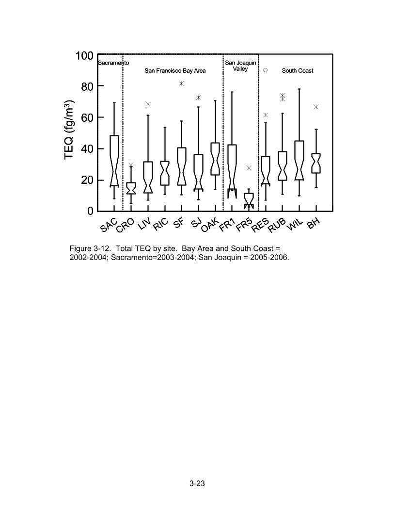
3-23

SACCRO LIV RIC SF SJ

OAKFR1

FR5RES

RUBWIL BH

SacramentoSan Francisco Bay Area

San JoaquinValley South Coast

TE

Q(f

g/m

3)

100

80

60

40

20

0

SACCRO LIV RIC SF SJ

OAKFR1

FR5RES

RUBWIL BH

SacramentoSan Francisco Bay Area

San JoaquinValley South Coast

TE

Q(f

g/m

3)

100

80

60

40

20

0

Figure 3-12. Total TEQ by site. Bay Area and South Coast = 2002-2004; Sacramento=2003-2004; San Joaquin = 2005-2006.

3-24

RES RUB WIL BH0

10

20

30

40

50T

EQ

(f g

/m3)

FuransDioxinsBiphenyls

CRO LIV RIC SF SJ OAK0

10

20

30

40

50

FR1 FR50

25

50

75

TE

Q (

f g/m

3)

SAC0

25

50

75

Figure 3-13. Total TEQ by parameter group and site (clockwise from top left): South Coast=2002-2004; Bay Area=2002-2004; San Joaquin=2005-2006; and Sacramento=2003-2004.

3-25

SACCRO LIV RIC SF SJ

OAKFR1

FR5RES

RUBWIL BH

0

20

40

60

80

Dio

xin

TE

Q (

fg/m

3)

SacramentoSan Francisco Bay Area

San JoaquinValley South Coast

SACCRO LIV RIC SF SJ

OAKFR1

FR5RES

RUBWIL BH

0

10

20

30

40

50

Fura

n T

EQ

(fg

/m3)

SacramentoSan Francisco Bay Area

San JoaquinValley South Coast

SACCRO LIV RIC SF SJ

OAKFR1

FR5RES

RUBWIL BH

0

5

10

15

20

25

Bip

hen y

l TE

Q (

fg/m

3 )

SacramentoSan Francisco Bay Area

San JoaquinValley South Coast

Figure 3-14. Individual TEQ for dioxins, furans, and biphenyls.

3-26

The Sacramento Valley and San Joaquin Valley Air Basin sites provided a more limited data set than did the other air basins, so confidence intervals when comparing among sites are large. The FR5 site concentrations are significantly lower than at any other site studied, and the site represents regional background, rather than urban influences. Dioxin concentrations at the Sacramento and Fresno First Street sites were similar to those observed in the San Francisco Bay Area and South Coast Air Basins. The biphenyl concentrations at the Sacramento and Fresno First Street sites were relatively high compared some of the sites in the San Francisco Bay Area and South Coast Air Basins. The furan concentrations at the Sacramento and Fresno First Street sites were lower than those at South Coast sites but similar to those at San Francisco Bay Area sites. Local sources may again be important for furans and biphenyls, especially in the South Coast.

Diphenylethers were also investigated by air basin and site, two different compounds are shown in Figures 3-15 and 3-16. The two compounds presented, 2,2’,3,3’4,4’5,5’6,6’-DecaBDE (DecaBDE) and 2,4-DiBDE (DiBDE2), are typical examples of spatial concentrations for diphenylethers. These compounds are highest in the South Coast overall, though Oakland and San Jose levels are higher than those in the rest of the Bay Area and similar to those in the South Coast. Rubidoux shows the highest concentrations, indicating these compounds may be influenced by sources that do not impact furan and biphenyl concentrations as much. Diphenylether concentrations were typically low in the San Joaquin Valley sites (Figure 3-16).

Overall spatial variability of biphenyl and diphenylether TEQ values was higher than that of dioxins and furans (Figure 3-14 and 3-16). The intra-urban differences of biphenyls and diphenylethers indicate that proximity to sources and/or meteorology is important in the ambient levels, and that one site in an air basin may not be representative of the entire air basin.

3-27

South Coast

Bay Area

San Joaquin

0

10000

20000

30000

40000

50000

60000

70000

80000

90000

100000

Con

cen

tra

tion

(fg

/m3 )

South Coast

Bay Area

San Joaquin

0

10000

20000

30000

40000

50000

60000

70000

80000

90000

100000

Con

cen

tra

tion

(fg

/m3 )

Figure 3-15. Spatial distribution of 2,2’,3,3’4,4’5,5’6,6’-DecaBDE (DecaBDE) concentrations by air basin which is typical of other diphenylethers. Diphenylethers were not monitored in Sacramento.

LIV SJ SFRIC

OAKFR1

FR5RUB

WIL BH

0

200

400

600

Con

cent

ratio

n (f

g/m

3 )

Bay Area

San Joaquin

South Coast

LIV SJ SFRIC

OAKFR1

FR5RUB

WIL BH

0

200

400

600

Con

cent

ratio

n (f

g/m

3 )

Bay Area

San Joaquin

South Coast

Figure 3-16. Spatial distribution of 2,4-DiBDE (DiBDE2) concentrations by site which is typical of other diphenylethers.

3-28

3.4.2 ANOVA Results

An ANOVA analysis provides a statistical measure of the similarity in average concentrations of compounds between air basins. The variability between groups (total TEQ for each group) is compared with the variability within each group (i.e., concentrations of each compound) to determine if differences between groups are real or within the noise of the data set. ANOVA between San Francisco Bay Area and South Coast Air Basins

Each compound and TEQ group (dioxins, furans, and biphenyls) were first compared between the Bay Area and South Coast Air Basins. The dioxin total TEQ did not show a significant dependence between these two air basins. Furan and biphenyl total TEQ did show a significant difference between these two air basins. This finding is consistent with the results when individual compounds were considered, that is, dioxin concentrations were not dependent on air basin while furan concentrations were different by air basin. Some biphenyls had a significant dependence on air basin and some did not. The variability within each air basin for furan and biphenyl concentrations is greater than that for dioxins which leads to these different results.

ANOVA was run again after Crockett site (CRO) data were removed because CRO had significantly different concentrations than other Bay Area sites and was thought to over-influence the ANOVA results. After removal of Crockett data, the results for TEQ groupings did not change; however, several compounds showed different results. Therefore, the Crockett site does not impact variation in total TEQ of any group, but does impact the variability of some compounds. These results indicate that as a whole, dioxin concentrations in the South Coast and Bay Area are not statistically significantly different, while furan and biphenyl concentrations are statistically significantly different. ANOVA results are summarized in Table 3-7.

ANOVA among Sites for all Air Basins

When all sites were considered, including sites from the Bay Area, South Coast, Sacramento Valley, and San Joaquin Air Basins, all TEQ groupings and all but two individual compounds showed a significant dependence on site. This result was expected because differences in concentration ranges among all sites were previously observed. When the Crockett site was removed from this analysis, the dioxins were no longer significantly dependent on site and four species that previously were dependent on site were no longer so. This result is likely because the Crockett site differed most from other sites in terms of concentration ranges; removing the Crockett site decreased the between-site variability.

3-29

Table 3-7. Analysis of variance results. S=Significant difference between sites; NS=insignificant difference between sites. Abbreviations are defined in Tables 2-1 through 2-4.

ANOVA Between Bay

Area and South Coast Air Basins

ANOVA Among Sites for All Air

Basins

ANOVA Among Sites for Individual Air Basins

Group or Compound

All Sites

All Sites Except CRO

All Sites

All Sites Except CRO

Bay Area

Bay Area

without CRO

South Coast

TEQD NS NS S NS S NS NS

TEQF S S S S S NS NS

TEQB S S S S S S S

TETCDD NS S S S S S S PECDD NS NS S S S S S HXCDD1 NS NS NS S S NS NS HXCDD2 NS NS S S S NS NS HXCDD3 NS NS S NS S NS S HPCDD NS NS S S S NS S OCDD NS NS S S S NS S TETCDF S S S S S S NS PECDF1 S NS S S S S NS PECDF2 S S S S S S NS HXCDF1 S NS NS S NS S NS HXCDF2 S S S NS S NS S HXCDF3 S S S S S S NS HXCDF4 S S S S S S NS HPCDF1 S S S S S S S HPCDF2 S S S S S S S OCDF S S S S S S NS TETCB1 NS NS S S S NS S TETCB2 NS NS S NS S NS S PECB1 S S S S S S S PECB2 NS S S S S S S PECB3 NS S S S S S S PECB4 NS NS S NS S NS S

PECB5 NS S S S S NS S HXCB1 S S S S S NS NS HXCB2 NS NS S S S NS S HXCB3 S NS S S S NS S HXCB4 NS NS S S S S S HPCB1 S S S S S S S HPCB2 S NS S S S S S

HPCB3 S NS S S S S S

3-30

ANOVA among Sites for Individual Air Basins

ANOVA was also performed among sites within the San Francisco Bay Area and South Coast Air Basins. Only one compound (1,2,3,7,8,9-HxCDF [HXCDF1]) within the Bay Area did not show a significant dependence on site. However, when the Crockett site was removed from analysis, 13 compounds and both the dioxin and furan TEQ groups no longer had a significant dependence on site. The Crockett site was largely responsible for the between-site variability in the Bay Area. When Crockett was removed from the analysis, Bay Area TEQ groups of dioxins and furans were statistically similar across sites as were about half the compounds.

When just the South Coast Air Basin sites were considered, the dioxin and furan TEQ groups, as well as many of the compounds, did not show significant dependence on site. The biphenyls as a group, and compounds except 3,3’4,4’5,5’-HxCB (HxCB1), had significant dependence on site; a higher percentage of HxCB1 data below is detection which probably influences the difference from other biphenyl compounds. This result implies the variability in concentrations of dioxins and furans is less than that of biphenyls in the South Coast Air Basin.

Figure 3-14 qualitatively agrees with the ANOVA results, and provides further insight into what caused the ANOVA results observed in Table 3-7. Notched box plots are based around median concentrations while ANOVA results are based on mean concentrations; agreement between the two statistical measures provides further confidence in the results. Overall, dioxin concentrations are very consistent across sites, furan concentrations have a little more variability, and biphenyl concentrations have high variability between sites.

3.4.3 Compound Profiles

Though some compounds showed spatially distinct concentration ranges, the relative fingerprints were similar among sites. Figure 3-17 shows an example fingerprint plot for each group. The y-axis indicates the fraction of the total mass from compounds within the group, for example, a value of 0.1 for 1,2,3,4,6,7,8-HpCDF (HpCDF1) would be interpreted to mean that HpCDF1 accounts for 10 percent of the total furan mass. The dioxin fingerprint is dominated by OCDD and 1,2,3,4,6,7,8-HpCDD (HpCDD), which account for an average of 26 and 7 percent of the total dioxin mass respectively. Furan fingerprints are also dominated by the higher chlorinated compounds with OCDF and HpCDF1 accounting for 10 and 13 percent of the total furan mass on average. The penta-chlorinated biphenyls account for the majority of the biphenyl mass with 2,3’,4,4’5-PeCB (PeCB3) at 19 percent and 2,3,3’,4,4’-PeCB (PeCB2) at 7 percent of the total mass; 2,2’3,4,4’5,5’-HpCB (HpCB2) accounts for an average of 5 percent of the total mass. 2,2’,4,4’-TetraBDE (TetBDE2) accounts for the most diphenylether mass with 13 percent, followed by 2,2’,3,3’,4,4’,5,5’,6,6’-DecaBDE (DecaBDE) and 2,2’,4,4’,5-PentaBDE (PeBDE3) at 8 percent each.

3-31

Dioxins Furans

OCDD

HpCDD

HxCDD1

HxCDD2

HxCDD3

PeCDD

TetCDD

0.00010

0.00100

0.01000

0.10000

1.00000

Fra

c tio

n o

f Co n

cent

rati o

n

OCDF

HpCDF1

HpCDF2

HxCDF1

HxCDF2

HxCDF3

HxCDF4

PeCDF1

PeCDF2

TetCDF

0.001

0.010

0.100

Fra

ctio

n of

Co

nce n

tra

tion

Biphenyls

HpCB1

HpCB2

HpCB3

HxCB1

HxCB2

HxCB3

HxCB4

PeCB1

PeCB2

PeCB3

PeCB4

PeCB5

TetCB1

TetCB2

0.00001

0.00010

0.00100

0.01000

0.10000

Fra

ctio

n o

f Con

cent

ratio

n

Diphenylethers

DecaBDE

NonBDE1

NonBDE2

NonBDE3OBDE

HpBDE1

HpBDE2

HpBDE3

HxBDE1

HxBDE2

HxBDE3

HxBDE4

HxBDE5

HxBDE6

PeBDE1

PeBDE2

PeBDE3

PeBDE4

PeBDE5

PeBDE6

PeBDE7

TetBDE1

TetBDE2

TetBDE3

TetBDE4

TetBDE5

TetBDE6

TetBDE7

TetBDE8

TriBDE1

TriBDE2

TriBDE4

TriBDE5

DiBDE1

DiBDE2

DiBDE3

DiBDE4

DiBDE5

TriBDE6

TriBDE3

0.00001

0.00010

0.00100

0.01000

0.10000

Fra

ctio

n of

Co n

cent

r atio

n

Figure 3-17. Relative contributions (fraction of concentration) to the total mass by group at the Rubidoux (RUB) monitoring site. Abbreviations are defined in Tables 2-1 through 2-4.

3-32

Diphenylethers at San Jose exhibited the only marked difference in the relative fingerprint profile. Figure 3-18 shows the San Jose diphenylether profile compared with the Rubidoux (typical) profile. The fingerprints are plotted on a linear scale to show the difference more clearly. In the San Jose fingerprint, the contribution of 2,2’,3,3’,4,4’,5,5’,6,6’-DecaBDE (DecaBDE) and 2,2’,4,4’-TetraBDE (TetBDE2) are less than half of the typical fingerprint while the contribution of 2,2’,4,4’,5-PentaBDE (PeBDE3) has increased to become the highest percentage of total mass (red circles). Note that fingerprints in Figure 3-18 look different than those in Figure 3-17 because they are plotted on a linear, rather than log, scale.

While absolute compound mass can vary, the distribution of compound mass (i.e., fingerprints) is very similar from site to site and sample to sample. The spatial and temporal similarity in compound fingerprints indicates that samples are aged. This similarity also means that analyses using either TEQ or concentrations will yield consistent results No information is being lost by using TEQ throughout the rest of this report.

3.5 TEMPORAL PATTERNS

3.5.1 Seasonal Patterns

Seasonal patterns of all compounds were investigated by site using notched box plots, which show the median concentration, with a 95 percent confidence interval, and give information about the distribution of concentrations. Concentrations of all compounds of dioxins and furans peaked in the cool seasons (September-February). Biphenyls generally exhibited a warm season (June-August) peak with two exceptions. The first was 3,3’,4,4’,5,5’-HxCB (HxCB1), which had a cool season peak, but had a high percent of data below detection at most sites (40-70 percent). However, HxCB1 showed a strong cool season peak at Sacramento, where only 24 percent of data were below detection. Because data below detection were reported as a zero and there were changes in the MDL throughout the study period, further investigation is necessary to determine if this trend is real or an artifact of the amount of data below detection. Another compound, 2,3,3’,4,4’,5,5’-HpCB (HpCB1) also exhibited a cool season peak at some sites (e.g., San Francisco, San Jose, Livermore, and Wilmington). Similar to HXCB1, a higher percentage of the HpCB1 data was below detection during the warm months and further investigation is needed to understand seasonal variability. An example of typical seasonal patterns is shown in Figure 3-19; biphenyl compounds that exhibit an atypical seasonal pattern are shown in Figure 3-20.

Because diphenylether data points at any given site were insufficient to create box plots and did not have WHO-97 TEFs, these compounds were examined by air basin. No diphenylether compounds had consistent seasonal trends between air basins, the patterns were typically weak compared with the dioxins and furans, and the trends were not consistent within parameter groups.

3-33

DecaBDE

NonBDE1

NonBDE2

NonBDE3

HpBDE1

HpBDE2

HpBDE3

HxBDE1

HxBDE2

HxBDE3

HxBDE4

HxBDE5

PeBDE1

PeBDE2

PeBDE3

PeBDE4

PeBDE5

PeBDE6

PeBDE7

TetBDE1

TetBDE2

TetBDE3

TetBDE4

TetBDE5

TetBDE6

TriBDE1

TriBDE2

TriBDE4

TriBDE5

DiBDE1

DiBDE2

DiBDE3

DiBDE4

DiBDE5

TriBDE6

TriBDE3

0.00

0.03

0.06

0.09

0.12

0.15

Fra

ctio

n of

Co n

cen t

ratio

n

SJ

DecaBDE

NonBDE1

NonBDE2

NonBDE3OBDE

HpBDE1

HpBDE2

HpBDE3

HxBDE1

HxBDE2

HxBDE3

HxBDE4

HxBDE5

HxBDE6

PeBDE1

PeBDE2

PeBDE3

PeBDE4

PeBDE5

PeBDE6

PeBDE7

TetBDE1

TetBDE2

TetBDE3

TetBDE4

TetBDE5

TetBDE6

TetBDE7

TetBDE8

TriBDE1

TriBDE2

TriBDE4

TriBDE5

DiBDE1

DiBDE2

DiBDE3

DiBDE4

DiBDE5

TriBDE6

TriBDE3

0.00

0.03

0.06

0.09

0.12

0.15F

ract

ion

of C

once

n tra

tion RUB (Typical)

DecaBDE

NonBDE1

NonBDE2

NonBDE3

HpBDE1

HpBDE2

HpBDE3

HxBDE1

HxBDE2

HxBDE3

HxBDE4

HxBDE5

PeBDE1

PeBDE2

PeBDE3

PeBDE4

PeBDE5

PeBDE6

PeBDE7

TetBDE1

TetBDE2

TetBDE3

TetBDE4

TetBDE5

TetBDE6

TriBDE1

TriBDE2

TriBDE4

TriBDE5

DiBDE1

DiBDE2

DiBDE3

DiBDE4

DiBDE5

TriBDE6

TriBDE3

0.00

0.03

0.06

0.09

0.12

0.15

Fra

ctio

n of

Co n

cen t

ratio

n

SJ

DecaBDE

NonBDE1

NonBDE2

NonBDE3OBDE

HpBDE1

HpBDE2

HpBDE3

HxBDE1

HxBDE2

HxBDE3

HxBDE4

HxBDE5

HxBDE6

PeBDE1

PeBDE2

PeBDE3

PeBDE4

PeBDE5

PeBDE6

PeBDE7

TetBDE1

TetBDE2

TetBDE3

TetBDE4

TetBDE5

TetBDE6

TetBDE7

TetBDE8

TriBDE1

TriBDE2

TriBDE4

TriBDE5

DiBDE1

DiBDE2

DiBDE3

DiBDE4

DiBDE5

TriBDE6

TriBDE3

0.00

0.03

0.06

0.09

0.12

0.15F

ract

ion

of C

once

n tra

tion RUB (Typical)

DecaBDE

NonBDE1

NonBDE2

NonBDE3

HpBDE1

HpBDE2

HpBDE3

HxBDE1

HxBDE2

HxBDE3

HxBDE4

HxBDE5

PeBDE1

PeBDE2

PeBDE3

PeBDE4

PeBDE5

PeBDE6

PeBDE7

TetBDE1

TetBDE2

TetBDE3

TetBDE4

TetBDE5

TetBDE6

TriBDE1

TriBDE2

TriBDE4

TriBDE5

DiBDE1

DiBDE2

DiBDE3

DiBDE4

DiBDE5

TriBDE6

TriBDE3

0.00

0.03

0.06

0.09

0.12

0.15

Fra

ctio

n of

Co n

cen t

ratio

n

SJ

DecaBDE

NonBDE1

NonBDE2

NonBDE3OBDE

HpBDE1

HpBDE2

HpBDE3

HxBDE1

HxBDE2

HxBDE3

HxBDE4

HxBDE5

HxBDE6

PeBDE1

PeBDE2

PeBDE3

PeBDE4

PeBDE5

PeBDE6

PeBDE7

TetBDE1

TetBDE2

TetBDE3

TetBDE4

TetBDE5

TetBDE6

TetBDE7

TetBDE8

TriBDE1

TriBDE2

TriBDE4

TriBDE5

DiBDE1

DiBDE2

DiBDE3

DiBDE4

DiBDE5

TriBDE6

TriBDE3

0.00

0.03

0.06

0.09

0.12

0.15F

ract

ion

of C

once

n tra

tion RUB (Typical)

Figure 3-18. The typical relative contribution to the total diphenylether mass (RUB) versus the atypical fingerprint at San Jose (SJ). Red circles indicate the species accounting for most of the difference. Abbreviations are defined in Tables 2-1 through 2-4.

3-34

HpCDF2

Winter

Spring

SummerFall

0.0

0.1

0.2

0.3

0.4

0.5

0.6

TE

Q (

fg/m

3)

OCDD

Winter

Spring

SummerFall

0.00

0.05

0.10

0.15

0.20

TE

Q (

fg/m

3)

PeCB2

Winter

Spring

SummerFall

0

1000

2000

3000

4000

5000

Con

cen

trat

i on

(fg

/ m3)

Figure 3-19. Example of seasonal patterns for HpCDF2, OCDD, and PeCB2 which are typical of furans, dioxins, and biphenyls respectively. Wilmington site data are illustrated; all sites show similar seasonal patterns. Abbreviations are defined in Tables 2-1 through 2-4.

3-35

HxCB1

Winter

Spring

SummerFall

0

5

10

15

20

25

Co

nce n

trat

i on

(fg /

m3

)HpCB1

Winter

Spring

SummerFall

0

10

20

30

40

50

60

70

Con

cent

rati o

n (f

g /m

3)

Figure 3-20. Example atypical seasonal patterns for HxCB1 and HpCB1. Wilmington site data are illustrated; all sites show similar seasonal patterns. Abbreviations are defined in Tables 2-1 through 2-4.

3.5.2 Inter-annual Patterns

Changes in median concentrations/TEQ were examined by year to determine if any annual trends were apparent. Because of the low number of available samples per year, significance tests were not appropriate and these results should be considered qualitative. Additionally, only two or three years of data were available (depending on site), which is not sufficient to constitute a trend. Total TEQ by Air Basin for Dioxins, Furans, and Biphenyls

Median annual TEQ for dioxins, furans, and biphenyls were examined by air basin (Figure 3-21). No distinct patterns were apparent at Bay Area and Sacramento sites over the years, but the median annual TEQs of all three groups at South Coast sites were higher in 2002. TEQs for dioxins and biphenyls appear to be decreasing by year in the South Coast Air Basin.

Total TEQ by Site for Dioxins, Furans, and Biphenyls

Median annual TEQs were also examined by site (Figure 3-22). Dioxins at Livermore were noticeably higher in 2003; in 2002 dioxins were noticeably higher at San Jose and Reseda. Dioxins and furans appear to be increasing by year at Oakland. Other noticeable differences in furans occur at San Jose, Reseda, and Rubidoux where furans were higher in 2002 than in subsequent years. Although changes in dioxin and

3-36

furan TEQs were similar, changes in biphenyls were not. Biphenyls in Richmond were low in 2002 and high at Boyle Heights in 2004.

Individual Species TEQ by Site for Dioxins, Furans, and Biphenyls

Fingerprint plots (median concentrations of each species within a compound group) were examined by year for each site. An example of a dioxin, furan, and biphenyl fingerprint plot for each air basin is shown in Figures 3-23 to 3-25. Overall, similar patterns/ratios were seen across years at all sites. Some deviations include higher dioxin and furan TEQs in 2002 at San Jose and Reseda, and some higher dioxin TEQs in 2003 at Livermore.

Diphenylether Concentrations by Site

Fingerprint plots were also examined for diphenylethers by year and site (Figure 3-26). Similar to the dioxin, furan, and biphenyl plots, ratios among diphenylether species were similar across years. The only group with a consistent change across sites was the NonaBDE group, which appears to be increasing. More analysis is necessary to determine the robustness of this result.

3.6 CORRELATIONS WITH PARALLEL AIR QUALITY MEASUREMENTS

Correlations of compound concentrations with other air quality parameters can provide insight into sources. For example, ambient benzene and toluene data are typically well correlated if a site is dominated by mobile sources, as they are both emitted in vehicle exhaust (Main et al., 1996; Brown et al., 2007). Parallel air quality measurements were available for some CADAMP sites and include a variety of parameters including criteria pollutants, VOCs, semi-volatile organic compounds (SVOCs), and speciated particulate measurements.

Site-level correlations were performed for Livermore and Rubidoux because these sites have the longest sampling period (2002-2005) and represent the San Francisco Bay Area and South Coast Air Basins. Additionally, regression statistics at San Jose were calculated in order to corroborate some results. One hundred thirty-seven parallel air quality parameters were available at Rubidoux, 30 were available at Livermore, and 105 were available at San Jose.

Dioxins and furans at Rubidoux showed the strongest correlation coefficient (R2) with zinc total suspended particulates (TSP). R2 values for dioxins and furans were between 0.5 and 0.8; however, only 12 data points (one year of data) were available for analysis. Measurements of TSP metals were also available at San Jose. The measurement time periods overlapped by only a few months, so comparisons could not be drawn, and other CADAMP sites did not measure TSP metals for the period of interest. Figure 3-27 shows scatter plots of zinc TSP versus OCDF and 1,2,3,6,7,8-HxCDD (HxCDD1) partitioned into warm (March-August) and cool (September-February). The correlation between OCDF and zinc TSP are upheld in the scatter plot (Figure 3-25a); the correlation with HxCDD1 is influenced by one high data point (Figure 3-25b). The seasonal pattern of dioxins and furans is similar to particulate

3-37

TEQD

0

2

4

6

8

10

12

Bay Area Sacramento South Coast

Me

dia

n T

EQ

(fg

/m3)

2002

2003

2004

TEQF

0

2

4

6

8

10

12

Bay Area Sacramento South Coast

Me

dia

n T

EQ

(fg

/m3)

2002

2003

2004

TEQB

0

1

2

3

4

5

6

7

8

Bay Area Sacramento South Coast

Me

dia

n T

EQ

(fg

/m3)

2002

2003

2004

Figure 3-21. Inter-annual patterns in median dioxin, furan, and biphenyl TEQs by air basin.

3-38

TEQD

0

5

10

15

20

25

CRO LIV OAK RIC SF SJ SAC BH RES RUB WIL

Me

dia

n T

EQ

(fg

/m3 )

TEQF

0

2

4

6

8

10

12

14

16

CRO LIV OAK RIC SF SJ SAC BH RES RUB WIL

Me

dia

n T

EQ

(fg

/m3 )

TEQB

0

2

4

6

8

10

12

CRO LIV OAK RIC SF SJ SAC BH RES RUB WIL

Me

dia

n T

EQ

(fg

/m3 )

2002

2003

2004

2002

2003

2004

2002

2003

2004

TEQD

0

5

10

15

20

25

CRO LIV OAK RIC SF SJ SAC BH RES RUB WIL

Me

dia

n T

EQ

(fg

/m3 )

TEQF

0

2

4

6

8

10

12

14

16

CRO LIV OAK RIC SF SJ SAC BH RES RUB WIL

Me

dia

n T

EQ

(fg

/m3 )

TEQB

0

2

4

6

8

10

12

CRO LIV OAK RIC SF SJ SAC BH RES RUB WIL

Me

dia

n T

EQ

(fg

/m3 )

2002

2003

2004

2002

2003

2004

2002

2003

2004

Figure 3-22. Inter-annual patterns in median dioxin, furan, and biphenyl TEQs by site.

3-39

2004

2003

2002

YEAR

2004

2003

2002

YEAR

OCDD

HpCDD

HxCDD1

HxCDD2

HxCDD3

PeCDD

TetCDD

0.01

0.10

1.00

10.00

Med

ian

TE

Q(f

g/m

3 )

OCDD

HpCDD

HxCDD1

HxCDD2

HxCDD3

PeCDD

TetCDD

0.01

0.10

1.00

10.00

Med

ian

TE

Q(f

g/m

3 )

OCDF

HpCDF1

HpCDF2

HxCDF1

HxCDF2

HxCDF3

HxCDF4

PeCDF1

PeCDF2

TetCDF

0.001

0.010

0.100

1.000

10.000

Med

ian

TE

Q(f

g/m

3 )

OCDF

HpCDF1

HpCDF2

HxCDF1

HxCDF2

HxCDF3

HxCDF4

PeCDF1

PeCDF2

TetCDF

0.001

0.010

0.100

1.000

10.000

Med

ian

TE

Q(f

g/m

3 )

HpCB1

HpCB2

HpCB3

HxCB1

HxCB2

HxCB3

HxCB4

PeCB1

PeCB2

PeCB3

PeCB4

PeCB5

TetCB1

TetCB2

0.0010

0.0100

0.1000

1.0000

Med

ian

TE

Q(f

g/m

3)

HpCB1

HpCB2

HpCB3

HxCB1

HxCB2

HxCB3

HxCB4

PeCB1

PeCB2

PeCB3

PeCB4

PeCB5

TetCB1

TetCB2

0.0010

0.0100

0.1000

1.0000

Med

ian

TE

Q(f

g/m

3)

Figure 3-23. Annual median fingerprint plots of compounds at San Jose (SJ). Abbreviations are defined in Tables 2-1 through 2-4.

3-40

2004

2003

2002

YEAR

2004

2003

2002

YEAR

OCDD

HpCDD

HxCDD1

HxCDD2

HxCDD3

PeCDD

TetCDD

0.01

0.10

1.00

10.00

Me

dia

n T

EQ

(fg/

m3 )

OCDD

HpCDD

HxCDD1

HxCDD2

HxCDD3

PeCDD

TetCDD

0.01

0.10

1.00

10.00

Me

dia

n T

EQ

(fg/

m3 )

OCDF

HpCDF1

HpCDF2

HxCDF1

HxCDF2

HxCDF3

HxCDF4

PeCDF1

PeCDF2

TetCDF

0.001

0.010

0.100

1.000

10.000

Me

dia

n T

EQ

(fg/

m3 )

OCDF

HpCDF1

HpCDF2

HxCDF1

HxCDF2

HxCDF3

HxCDF4

PeCDF1

PeCDF2

TetCDF

0.001

0.010

0.100

1.000

10.000

Me

dia

n T

EQ

(fg/

m3 )

HpCB1

HpCB2

HpCB3

HxCB1

HxCB2

HxCB3

HxCB4

PeCB1

PeCB2

PeCB3

PeCB4

PeCB5

TetCB1

TetCB2

0.0010

0.0100

0.1000

1.0000

Med

ian

TE

Q(f

g/m

3)

HpCB1

HpCB2

HpCB3

HxCB1

HxCB2

HxCB3

HxCB4

PeCB1

PeCB2

PeCB3

PeCB4

PeCB5

TetCB1

TetCB2

0.0010

0.0100

0.1000

1.0000

Med

ian

TE

Q(f

g/m

3)

Figure 3-24. Annual median fingerprint plots of compounds at Reseda (RES). Abbreviations are defined in Tables 2-1 through 2-4.

3-41

2004

2003

2002

YEAR

2004

2003

2002

YEAR

OCDD

HpCDD

HxCDD1

HxCDD2

HxCDD3

PeCDD

TetCDD

0.010

0.100

1.000

10.000

Med

ian

TE

Q(f

g/m

3 )

OCDD

HpCDD

HxCDD1

HxCDD2

HxCDD3

PeCDD

TetCDD

0.010

0.100

1.000

10.000

Med

ian

TE

Q(f

g/m

3 )

OCDF

HpCDF1

HpCDF2

HxCDF1

HxCDF2

HxCDF3

HxCDF4

PeCDF1

PeCDF2

TetCDF

0.0010

0.0100

0.1000

1.0000

10.0000

Med

ian

TE

Q(f

g/m

3 )

OCDF

HpCDF1

HpCDF2

HxCDF1

HxCDF2

HxCDF3

HxCDF4

PeCDF1

PeCDF2

TetCDF

0.0010

0.0100

0.1000

1.0000

10.0000

Med

ian

TE

Q(f

g/m

3 )

HpCB1

HpCB2

HpCB3

HxCB1

HxCB2

HxCB3

HxCB4

PeCB1

PeCB2

PeCB3

PeCB4

PeCB5

TetCB1

TetCB2

0.0010

0.0100

0.1000

1.0000

Med

ian

TE

Q(f

g/m

3 )

HpCB1

HpCB2

HpCB3

HxCB1

HxCB2

HxCB3

HxCB4

PeCB1

PeCB2

PeCB3

PeCB4

PeCB5

TetCB1

TetCB2

0.0010

0.0100

0.1000

1.0000

Med

ian

TE

Q(f

g/m

3 )

Figure 3-25. Annual median fingerprint plots of compounds at Livermore (LIV). Abbreviations are defined in Tables 2-1 through 2-4.

3-42

RIC

DecaBDE

NonBDE

HpBDE

HxBDE

PeBDE

TetBDE

TriBDE

DiBDE

1000

10000

100000

1000000M

edia

n C

once

ntra

tion

(fg/

m3 )

RIC

DecaBDE

NonBDE

HpBDE

HxBDE

PeBDE

TetBDE

TriBDE

DiBDE

1000

10000

100000

1000000M

edia

n C

once

ntra

tion

(fg/

m3 )

OAK

DecaBDE

NonBDE

HpBDE

HxBDE

PeBDE

TetBDE

TriBDE

DiBDE100

1000

10000

100000

1000000

Med

ian

Con

cent

ratio

n (f

g/m

3 )

OAK

DecaBDE

NonBDE

HpBDE

HxBDE

PeBDE

TetBDE

TriBDE

DiBDE100

1000

10000

100000

1000000

Med

ian

Con

cent

ratio

n (f

g/m

3 )

SF

DecaBDE

NonBDE

HpBDE

HxBDE

PeBDE

TetBDE

TriBDE

DiBDE

100

1000

10000

100000

1000000

Med

ian

Con

cent

ratio

n (

fg/m

3 )

SF

DecaBDE

NonBDE

HpBDE

HxBDE

PeBDE

TetBDE

TriBDE

DiBDE

100

1000

10000

100000

1000000

Med

ian

Con

cent

ratio

n (

fg/m

3 )

SJ

DecaBDE

NonBDE

HpBDE

HxBDE

PeBDE

TetBDE

TriBDE

DiBDE

1000

10000

100000

1000000

Med

ian

Con

cent

ratio

n (f

g/m

3 )

SJ

DecaBDE

NonBDE

HpBDE

HxBDE

PeBDE

TetBDE

TriBDE

DiBDE

1000

10000

100000

1000000

Med

ian

Con

cent

ratio

n (f

g/m

3 )

WIL

DecaBDE

NonBDE

HpBDE

HxBDE

PeBDE

TetBDE

TriBDE

DiBDE

1000

10000

100000

1000000

Med

ian

Con

cent

ratio

n (f

g/m

3 )

WIL

DecaBDE

NonBDE

HpBDE

HxBDE

PeBDE

TetBDE

TriBDE

DiBDE

1000

10000

100000

1000000

Med

ian

Con

cent

ratio

n (f

g/m

3 )

BH

DecaBDE

NonBDE

HpBDE

HxBDE

PeBDE

TetBDE

TriBDE

DiBDE1000

10000

100000

1000000

Med

ian

Con

cent

ratio

n (f

g/m

3 )

BH

DecaBDE

NonBDE

HpBDE

HxBDE

PeBDE

TetBDE

TriBDE

DiBDE1000

10000

100000

1000000

Med

ian

Con

cent

ratio

n (f

g/m

3 )

RUB

DecaBDE

NonBDE

HpBDE

HxBDE

PeBDE

TetBDE

TriBDE

DiBDE

1000

10000

100000

1000000

Me

dia

n C

on

cen

tra

tion

(fg

/m3)

RUB

DecaBDE

NonBDE

HpBDE

HxBDE

PeBDE

TetBDE

TriBDE

DiBDE

1000

10000

100000

1000000

Me

dia

n C

on

cen

tra

tion

(fg

/m3)

200520042003

YEAR

200520042003

YEAR

Figure 3-26. Inter-annual patterns in median concentrations of diphenylethers by site. Abbreviations are defined in Tables 2-1 through 2-4.

3-43

pollution (i.e., zinc TSP); therefore, seasonality may be influencing this correlation. However, biphenyls have the opposite seasonal pattern to dioxins and furans, but show no correlation with zinc TSP (Figure 3-25c). If the correlation were dependant on seasonal variability alone, biphenyls should show a negative correlation with zinc TSP. This pattern is observed in correlations with zinc PM2.5 (Figure 3-28), indicating that the relationship with zinc PM2.5 may be a result of similar seasonal patterns, while the correlation with zinc TSP may be the result of similar emissions sources.

The zinc emissions near Rubidoux during 2004 were investigated along with wind roses (2002-2004 data) to identify local sources of zinc (Figure 3-29). Major zinc emission sources were located about six miles northwest of the Rubidoux site, and prevailing winds were frequently from the direction of these sources; more data are necessary to corroborate this finding. Major zinc sources near Rubidoux include wire production and refining activities. Additional local sources of zinc may include tire wear, which emits as much zinc as medical waste incinerators in the US (Councell et al., 2004).

Biphenyls at Rubidoux did not show strong correlations with any species but showed fair correlations with ozone, phosphorous TSP, all particulate sulfate size fractions (PM10, PM2.5, TSP), and sulfur PM2.5, although correlation coefficients were never greater than 0.65. Scatter plots of these air quality parameters and dioxins, furans, and biphenyls indicate that correlations were influenced by similarity in seasonal patterns, as dioxins and furans showed a weak negative correlation. Figure 3-30 shows scatter plots of biphenyls and furans with sulfur PM2.5 at Rubidoux; a weak to fair correlation of biphenyls with sulfur PM2.5 was also indicated at San Jose (R2=0.1-0.6). Though seasonality may be a factor, the positive correlation of sulfur PM2.5 with biphenyls seems stronger and further investigation in warranted.

Correlations at San Jose showed a strong relationship (R2 typically above 0.9) between black carbon PM2.5 and both furans and dioxins. Unfortunately, again, only limited data were available for comparison and no other sites provided available black carbon measurements to corroborate this finding. Black carbon is emitted as a product of fuel combustion including wood, but in California urban areas, it can be related to mobile source emissions, especially diesel. Other air quality parameters related to mobile sources were available for comparison. Figure 3-31 shows the relationship between black carbon PM2.5, elemental carbon PM2.5, and typical dioxin and furan species. Though correlation coefficients for elemental carbon were low, Figure 3-31 shows a good relationship between elemental carbon and dioxins and furans. Low correlation coefficients were likely influenced by a single outlier point. Based on the scatter plots, furans seem to have a more linear relationship with elemental and black carbon than do dioxins; dioxin concentrations appear to level off at higher carbon concentrations. These relationships point to a mobile source influence for both dioxins and furans, though the low number of data points and strong seasonal patterns contribute to uncertainty in this conclusion.

Correlation coefficients at Livermore did not show strong relationships. This result is primarily because the compounds that did show relationships at the other sites, such as TSP metals and black carbon, were not measured at Livermore.

3-44

HxC

DD

1 (f

g/m

3)

Zinc TSP (µg/m3)

R2=0.70O

CD

F (

fg/m

3)

Zinc TSP (µg/m3)

R2=0.76

0.00 0.05 0.10 0.15 0.200

10

20

30

40

50

60

70

80

90

0.00 0.05 0.10 0.15 0.200

10

20

30

40

50

60

WarmCool

SEASON

Furan Dioxin

Pe

CB

3 (

fg/m

3 )

Zinc TSP (µg/m3)

R2=0.040

Biphenyl

0.00 0.05 0.10 0.15 0.200

50

100

150

200

HxC

DD

1 (f

g/m

3)

Zinc TSP (µg/m3)

R2=0.70O

CD

F (

fg/m

3)

Zinc TSP (µg/m3)

R2=0.76

0.00 0.05 0.10 0.15 0.200

10

20

30

40

50

60

70

80

90

0.00 0.05 0.10 0.15 0.200

10

20

30

40

50

60

WarmCool

SEASON

WarmCool

SEASON

Furan Dioxin

Pe

CB

3 (

fg/m

3 )

Zinc TSP (µg/m3)

R2=0.040

Biphenyl

0.00 0.05 0.10 0.15 0.200

50

100

150

200

Pe

CB

3 (

fg/m

3 )

Zinc TSP (µg/m3)

R2=0.040

Biphenyl

0.00 0.05 0.10 0.15 0.200

50

100

150

200

(a) (b)

(c)

Figure 3-27. Correlations between zinc TSP and example (a) furan, (b) dioxin, and (c) biphenyl parameters at Rubidoux (n=12). Red indicates warm seasons (March-August); blue indicates cool seasons (September-February). Abbreviations are defined in Tables 2-1 through 2-4.

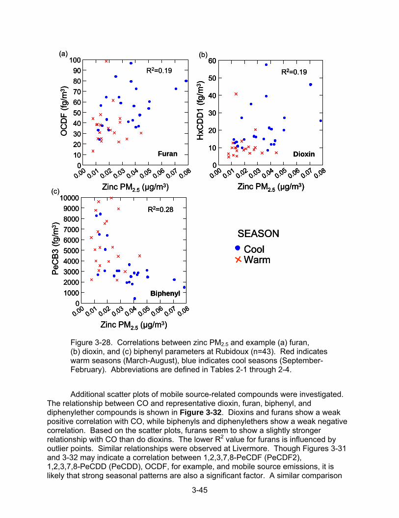
3-45

WarmCool

SEASON

0.000.01

0.020.03

0.040.05

0.060.07

0.08

Zinc PM2.5 (µg/m3)

0

10

20

30

40

50

60

70

80

90

100O

CD

F (

fg/m

3 )R2=0.19

Furan

0.000.01

0.020.03

0.040.05

0.060.07

0.08

Zinc PM2.5 (µg/m3)

0

10

20

30

40

50

60

HxC

DD

1 (f

g/m

3 )

R2=0.19

Dioxin

0.000.01

0.020.03

0.040.05

0.060.07

0.08

Zinc PM2.5 (µg/m3)

0

1000

2000

3000

4000

5000

6000

7000

8000

9000

10000

PeC

B3

(fg/

m3)

R2=0.28

Biphenyl

(a) (b)

(c)

WarmCool

SEASON

WarmCool

SEASON

0.000.01

0.020.03

0.040.05

0.060.07

0.08

Zinc PM2.5 (µg/m3)

0

10

20

30

40

50

60

70

80

90

100O

CD

F (

fg/m

3 )

0.000.01

0.020.03

0.040.05

0.060.07

0.08

Zinc PM2.5 (µg/m3)

0

10

20

30

40

50

60

70

80

90

100O

CD

F (

fg/m

3 )R2=0.19

Furan

0.000.01

0.020.03

0.040.05

0.060.07

0.08

Zinc PM2.5 (µg/m3)

0

10

20

30

40

50

60

HxC

DD

1 (f

g/m

3 )

R2=0.19

Dioxin

0.000.01

0.020.03

0.040.05

0.060.07

0.08

Zinc PM2.5 (µg/m3)

0

10

20

30

40

50

60

HxC

DD

1 (f

g/m

3 )

0.000.01

0.020.03

0.040.05

0.060.07

0.08

Zinc PM2.5 (µg/m3)

0

10

20

30

40

50

60

HxC

DD

1 (f

g/m

3 )

R2=0.19

Dioxin

0.000.01

0.020.03

0.040.05

0.060.07

0.08

Zinc PM2.5 (µg/m3)

0

1000

2000

3000

4000

5000

6000

7000

8000

9000

10000

PeC

B3

(fg/

m3)

R2=0.28

Biphenyl

0.000.01

0.020.03

0.040.05

0.060.07

0.08

Zinc PM2.5 (µg/m3)

0

1000

2000

3000

4000

5000

6000

7000

8000

9000

10000

PeC

B3

(fg/

m3)

R2=0.28

Biphenyl

(a) (b)

(c)

Figure 3-28. Correlations between zinc PM2.5 and example (a) furan, (b) dioxin, and (c) biphenyl parameters at Rubidoux (n=43). Red indicates warm seasons (March-August), blue indicates cool seasons (September-February). Abbreviations are defined in Tables 2-1 through 2-4.

Additional scatter plots of mobile source-related compounds were investigated. The relationship between CO and representative dioxin, furan, biphenyl, and diphenylether compounds is shown in Figure 3-32. Dioxins and furans show a weak positive correlation with CO, while biphenyls and diphenylethers show a weak negative correlation. Based on the scatter plots, furans seem to show a slightly stronger relationship with CO than do dioxins. The lower R2 value for furans is influenced by outlier points. Similar relationships were observed at Livermore. Though Figures 3-31 and 3-32 may indicate a correlation between 1,2,3,7,8-PeCDF (PeCDF2), 1,2,3,7,8-PeCDD (PeCDD), OCDF, for example, and mobile source emissions, it is likely that strong seasonal patterns are also a significant factor. A similar comparison

3-46

with NOx was not performed because while NOx is emitted by mobile sources, there are also other significant sources of NOx.

Figure 3-29. Toxics release inventory (U.S. Environmental Protection Agency, 2004) of zinc point emissions in 2004 and 2002-2004 wind data at Rubidoux.

Dioxins, furans, biphenyls, and diphenylethers are semi-volatile and are therefore thought to partition between the gas and particulate phase. The highest chlorinated compounds have the lowest vapor pressures and are expected to be more heavily associated with PM (Lohmann and Jones, 1998). Based on regression statistics, there was no correlation between compounds and PM mass. This lack of correlation is upheld in Figure 3-33 where scatter plots between PM2.5, PM10, and higher chlorinated compounds show no correlation. Similar patterns were observed at Livermore. This lack of correlation is likely a function of the difference in sampling schedule between compounds and PM. The 28-day dioxins sample constitutes a sum of concentrations, while PM measurements are an average of 24-hr samples collected every third or sixth day. Therefore, the PM measurements only capture a fraction of the 28-day time period and many concentration events are lost. This lack of correlation should not be considered evidence of a lack of association between these compounds and PM.

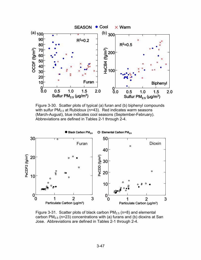
3-47

0.0 0.5 1.0 1.5 2.0Sulfur PM2.5 (µg/m3)

0

100

200

300

HxC

B4 (

fg/m

3 )

R2=0.5

Biphenyl

R2=0.2

0.0 0.5 1.0 1.5 2.0Sulfur PM2.5 (µg/m3)

0102030405060708090

100O

CD

F (

fg/m

3 )

Furan

SEASON Cool Warm(a) (b)

0.0 0.5 1.0 1.5 2.0Sulfur PM2.5 (µg/m3)

0

100

200

300

HxC

B4 (

fg/m

3 )

R2=0.5

Biphenyl

0.0 0.5 1.0 1.5 2.0Sulfur PM2.5 (µg/m3)

0

100

200

300

HxC

B4 (

fg/m

3 )

R2=0.5

Biphenyl

R2=0.2

0.0 0.5 1.0 1.5 2.0Sulfur PM2.5 (µg/m3)

0102030405060708090

100O

CD

F (

fg/m

3 )

Furan

R2=0.2

0.0 0.5 1.0 1.5 2.0Sulfur PM2.5 (µg/m3)

0102030405060708090

100O

CD

F (

fg/m

3 )

Furan

SEASON Cool WarmSEASON Cool Warm(a) (b)

Figure 3-30. Scatter plots of typical (a) furan and (b) biphenyl compounds with sulfur PM2.5 at Rubidoux (n=43). Red indicates warm seasons (March-August), blue indicates cool seasons (September-February). Abbreviations are defined in Tables 2-1 through 2-4.

PeC

DF

2 (f

g/m

3)

Particulate Carbon (µg/m3)

PeC

DD

(fg/

m3)

Particulate Carbon (µg/m3)0 1 2 3

0

10

20

30

Black Carbon PM2.5 Elemental Carbon PM2.5

0 1 2 30

10

20

30

40

50

PeC

DF

2 (f

g/m

3)

Particulate Carbon (µg/m3)

PeC

DD

(fg/

m3)

Particulate Carbon (µg/m3)0 1 2 3

0

10

20

30

Black Carbon PM2.5 Elemental Carbon PM2.5Black Carbon PM2.5 Elemental Carbon PM2.5

0 1 2 30

10

20

30

40

50Furan Dioxin

Figure 3-31. Scatter plots of black carbon PM2.5 (n=8) and elemental carbon PM2.5 (n=23) concentrations with (a) furans and (b) dioxins at San Jose. Abbreviations are defined in Tables 2-1 through 2-4.

3-48

R2=0.26

R2=0.17

0.2 0.4 0.6 0.8 1.0 1.2Carbon Monoxide (ppm)

0

1000

2000

3000O

CD

D (

fg/m

3 )

R2=0.14

0.2 0.4 0.6 0.8 1.0 1.2Carbon Monoxide (ppm)

0

10

20

30

40

50

60

70

80

90

100

OC

DF

(fg

/m3 )

0.2 0.4 0.6 0.8 1.0 1.2Carbon Monoxide (ppm)

0

100

200

300

HxC

B4

(fg/

m3 )

R2=0.27

0.2 0.4 0.6 0.8 1.0 1.2Carbon Monoxide (ppm)

0

1000

2000

3000

4000

5000

6000

7000N

onB

DE

1 (

fg/m

3 )

Season Cool Warm

(a)

(c)

(b)

(d)

R2=0.26

R2=0.17

0.2 0.4 0.6 0.8 1.0 1.2Carbon Monoxide (ppm)

0

1000

2000

3000O

CD

D (

fg/m

3 )

R2=0.14

0.2 0.4 0.6 0.8 1.0 1.2Carbon Monoxide (ppm)

0

10

20

30

40

50

60

70

80

90

100

OC

DF

(fg

/m3 )

R2=0.14

0.2 0.4 0.6 0.8 1.0 1.2Carbon Monoxide (ppm)

0

10

20

30

40

50

60

70

80

90

100

OC

DF

(fg

/m3 )

0.2 0.4 0.6 0.8 1.0 1.2Carbon Monoxide (ppm)

0

100

200

300

HxC

B4

(fg/

m3 )

0.2 0.4 0.6 0.8 1.0 1.2Carbon Monoxide (ppm)

0

100

200

300

HxC

B4

(fg/

m3 )

R2=0.27

0.2 0.4 0.6 0.8 1.0 1.2Carbon Monoxide (ppm)

0

1000

2000

3000

4000

5000

6000

7000N

onB

DE

1 (

fg/m

3 )R2=0.27

0.2 0.4 0.6 0.8 1.0 1.2Carbon Monoxide (ppm)

0

1000

2000

3000

4000

5000

6000

7000N

onB

DE

1 (

fg/m

3 )

Season Cool WarmSeason Cool Warm

(a)

(c)

(b)

(d)

Figure 3-32. Scatter plots of carbon monoxide and representative (a) dioxin, (b) furan, (c) biphenyl, and (d) diphenylether compounds at Rubidoux (n=30-42). Red indicates warm seasons (March-August); blue indicates cool seasons (September-February). Abbreviations are defined in Tables 2-1 through 2-4.

3-49

OC

DF

(fg/

m3 )

10 20 30 40 5010

20

30

40

50

60

70

80

90

100

10 20 30 40 5010

20

30

40

50

60

70

80

90

100

40

2000

PM2.5 (µg/m3) PM2.5 (µg/m3)

PM10 (µg/m3) PM10 (µg/m3) PM10 (µg/m3)

PM2.5 (µg/m3)

Non

BD

E1

(fg/

m3 )

HxC

B4

(fg/

m3 )

HxC

B4

(fg/

m3 )

OC

DF

(fg/

m3 )

20 30 40 50 60 70 80 900

1000

2000

3000

20 30 40 50 60 70 80 900

1000

2000

3000

20 30 40 50 60 70 80 9010

20

30

40

50

60

70

80

90

100

20 30 40 50 60 70 80 9010

20

30

40

50

60

70

80

90

100

20 30 40 50 60 70 80 900

100

200

300

20 30 40 50 60 70 80 900

100

200

300

20 30 50 60 70 80 900

1000

3000

4000

5000

6000

7000

10 20 30 40 500

100

200

300

10 20 30 40 500

100

200

300

10 20 30 40 500

1000

2000

3000

4000

5000

6000

7000

10 20 30 40 500

1000

2000

3000

4000

5000

6000

7000Dioxin Furan Biphenyl Diphenylether

PM10 (µg/m3)

OC

DD

(fg/

m3 )

R2=0.005

PM2.5 (µg/m3)

OC

DD

(fg/

m3 )

R2=0.03

R2=0.02 R2=0.08

R2=0.01

R2=0.3 R2=0.2

Non

BD

E1

(fg/

m3 )

R2=0.005

10 20 30 40 500

1000

2000

3000

10 20 30 40 500

1000

2000

3000

SEASON Cool WarmSEASON Cool Warm

Figure 3-33. Representative dioxin, furan, biphenyl, and diphenylether correlations with PM2.5 (n=42) and PM10 (n=40) at Rubidoux. Red indicates warm seasons (March-August); blue indicates cool seasons (September-February). Compound abbreviations are defined in Tables 2-1 through 2-4.

There is also evidence that soil can act as a reservoir for dioxins, furans, and biphenyls (Cleverly et al., 1999). Though regression statistics did not indicate a correlation, scatter plots of particulate soil markers (e.g., silicon, calcium) were investigated. Collection differences discussed previously between PM species and CADAMP monitoring likely affect these correlations as well. Figure 3-34 shows correlations between silicon PM2.5 and measured compounds. While correlations are not apparent, Pearson correlation coefficients (R) for dioxin, furan, and biphenyl are positive. The relationship between silicon and dioxins, furans, and biphenyls may be overcoming the strong seasonal differences among the compounds, indicating some correlation. This lack of correlation should not be considered evidence of a lack of association between these compound groups and soil and crustal markers due to the difference in the sampling schedule between CADAMP and PM. More investigation into the effect of sampling schedule differences is needed.

3.7 SUMMARY

A variety of analytical tools were used to characterize spatial and temporal patterns, place CADAMP concentrations into national perspective, investigate the relationship between rural and urban concentrations, and identify potential sources. The behavior of dioxins, furans, and biphenyls was generally consistent within their respective compound classes, while diphenylethers showed inconsistent results among

3-50

compounds and sites. This observation is likely explained by a combination of more data below detection, fewer available samples, and lower confidence in sampling methods as indicated by the analysis of collocated data.

0.0 0.1 0.2 0.3 0.40

1000

2000

3000

4000

5000

6000

7000

0.0 0.1 0.2 0.3 0.40

100

200

300

0.0 0.1 0.2 0.3 0.40

10

20

30

40

50

60

70

80

90

100

0.0 0.1 0.2 0.3 0.40

1000

2000

3000

Non

BD

E1

(fg

/m3 )

Silicone PM2.5 (µg/m3)

R2=0.02

OC

DD

(fg

/m3 )

Silicone PM2.5 (µg/m3)

R2=0.01

OC

DF

(fg

/m3 )

Silicone PM2.5 (µg/m3)

R2=0.09

Silicone PM2.5 (µg/m3)

HxC

B4

(fg

/m3 )

R2=0.03

Season Cool WarmSeason Cool Warm

Figure 3-34. Scatter plots of OCDD, OCDF, HxCB4, and NonBDE1 and silicon PM2.5 at Rubidoux (n=42). Red indicates warm seasons (March-August); blue indicates cool seasons (September-February). Abbreviations are defined in Tables 2-1 through 2-4.

Highlights of Findings

Dioxins and furans showed similar behavior in most analyses. The highest concentrations occurred in cool months and lowest concentrations in warm months, consistent with seasonal influence of ventilation, and consistent emissions sources throughout the year. Total dioxin TEQ and furan TEQ were similar among sites within an air basin. Concentrations in the South Coast Air Basin were slightly higher than concentrations in the San Francisco Bay Area Air

3-51

Basin. The FR5 site, which is the only rural site, had the lowest measured TEQ for biphenyls and furans.

Biphenyls exhibited different behavior than dioxins and furans. Biphenyl concentrations showed a seasonal pattern that peaked in warm months and were lowest in cool months. Concentrations of biphenyls were highly variable across sites, indicating ambient concentrations may be impacted by local sources and/or reactivity. Similar to dioxins and furans, ambient concentrations in the South Coast Air Basin were slightly higher than those in the Bay Area Air Basin; and the lowest ambient concentrations occurred at the FR5 monitoring site.

Concentrations (TEQ) of dioxins, furans, and biphenyls in California are typically one to two times higher than at other urban sites nationally. Though the NDAMN network only conducts four samples per year, thus only capturing one-third of the number of samples measured by the CADAMP network, the NDAMN data set provided useful comparisons to national concentrations of dioxins and differences among urban, rural, and remote compound profiles. Rural NDAMN concentrations of dioxins, furans, and biphenyls were equal to about 60 percent, 40 percent, and 10 percent of urban concentrations, respectively. In contrast, remote NDAMN concentrations of dioxin, furan, and biphenyl compounds were consistently about 5 percent of urban concentrations. The similarity in the fraction of remote concentrations among dioxins, furans, and biphenyls indicates a comparable lifetime, while the dissimilarity in the fraction of rural concentrations may indicate that there are more rural sources of dioxins and furans than biphenyls.

Mobile sources are likely an important contributor to dioxin and furan concentrations. Correlations with air quality parameters such as black carbon, elemental carbon PM2.5, and CO indicated mobile sources of dioxins and furans. Strong correlations with zinc TSP at one site implicated local sources of dioxins and furans; TSP metals data were not available at other sites for comparison. Dioxins, furans, biphenyls, and diphenylethers did not show a relationship with soil and crustal markers such as silicon and calcium. However, this lack of correlation should not be considered evidence of a lack of association between these compound groups and soil and crustal markers due to the difference in the sampling schedule between CADAMP and PM. The similarity in effect of ventilation index on all parameters and differences in sampling frequency among networks may influence these results.

Further investigation of the impact of meteorology on seasonal patterns as well as the potential sources of dioxins, furans, biphenyls, and diphenylethers will be discussed in Sections 4 and 5 of this report.

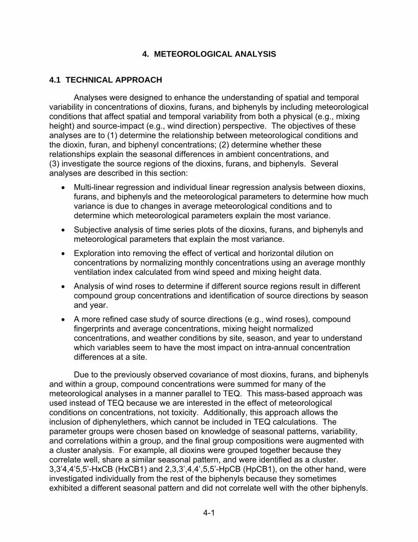
4-1

4. METEOROLOGICAL ANALYSIS

4.1 TECHNICAL APPROACH

Analyses were designed to enhance the understanding of spatial and temporal variability in concentrations of dioxins, furans, and biphenyls by including meteorological conditions that affect spatial and temporal variability from both a physical (e.g., mixing height) and source-impact (e.g., wind direction) perspective. The objectives of these analyses are to (1) determine the relationship between meteorological conditions and the dioxin, furan, and biphenyl concentrations; (2) determine whether these relationships explain the seasonal differences in ambient concentrations, and (3) investigate the source regions of the dioxins, furans, and biphenyls. Several analyses are described in this section:

Multi-linear regression and individual linear regression analysis between dioxins, furans, and biphenyls and the meteorological parameters to determine how much variance is due to changes in average meteorological conditions and to determine which meteorological parameters explain the most variance.

Subjective analysis of time series plots of the dioxins, furans, and biphenyls and meteorological parameters that explain the most variance.

Exploration into removing the effect of vertical and horizontal dilution on concentrations by normalizing monthly concentrations using an average monthly ventilation index calculated from wind speed and mixing height data.

Analysis of wind roses to determine if different source regions result in different compound group concentrations and identification of source directions by season and year.

A more refined case study of source directions (e.g., wind roses), compound fingerprints and average concentrations, mixing height normalized concentrations, and weather conditions by site, season, and year to understand which variables seem to have the most impact on intra-annual concentration differences at a site.

Due to the previously observed covariance of most dioxins, furans, and biphenyls and within a group, compound concentrations were summed for many of the meteorological analyses in a manner parallel to TEQ. This mass-based approach was used instead of TEQ because we are interested in the effect of meteorological conditions on concentrations, not toxicity. Additionally, this approach allows the inclusion of diphenylethers, which cannot be included in TEQ calculations. The parameter groups were chosen based on knowledge of seasonal patterns, variability, and correlations within a group, and the final group compositions were augmented with a cluster analysis. For example, all dioxins were grouped together because they correlate well, share a similar seasonal pattern, and were identified as a cluster. 3,3’4,4’5,5’-HxCB (HxCB1) and 2,3,3’,4,4’,5,5’-HpCB (HpCB1), on the other hand, were investigated individually from the rest of the biphenyls because they sometimes exhibited a different seasonal pattern and did not correlate well with the other biphenyls.

4-2

Similar to TEQ, the completeness criterion required that each compound within a group be present.

4.1.1 Dioxins Cluster Analysis and Parameter Groupings

Before performing cluster analysis to compound groups, compounds with greater than 55 percent of data below detection overall were removed. These compounds included 2,4,6-TriBDE3 (TriBDE3), 3,3’,4-TriBDE (TriBDE6), 2,3,4,5,6-PentaBDE (PeBDE4), 2,3,3',4,4'-PentaBDE (PeBDE6), 2,4',6-TriBDE (TriBDE5), 3,3',4,4',5-PentaBDE (PeBDE7), 2,2',3,3',4,4'-HexaBDE (HxBDE6), and 2,6-DiBDE (DiBDE1). Cluster analysis was performed on the remaining compounds in SYSTAT using the Euclidean distance and the nearest neighbor linkage (also known as “single” linkage). This method uses the two nearest neighbors within a group to calculate the Euclidean distance (i.e., geometric distance) between the clusters. A smaller distance indicates that compounds are more similar (StatSoft, 2004).

Cluster results are shown in Figure 4-1. Overall, compounds are grouped by type and color-coded: dioxins in red, furans in orange, biphenyls in yellow, and diphenylethers in blue and green. Outlier compounds are those that have the largest Euclidean distance (e.g., 2,2',4,4',6-PentaBDE [PeBDE2]), and are typically not grouped near other compounds of the same type. The final groupings used in subsequent meteorological analyses are listed in Table 4-1 along with a description of why the compounds were grouped. The disparate behavior of 3,3’4,4’5,5’-HxCB (HxCB1) and 1,2,3,7,8,9-HxCDF (HxCDF1) from their groups was influenced by the amount of data below detection; therefore, these compounds are not discussed in the analyses.

4.1.2 Meteorological Parameters

To investigate the relationship between meteorology and dioxins, furans, and biphenyls, we used a meteorological data set that contains over 120 observed, modeled, and calculated meteorological and transport parameters available near several sites within each sampling region for the period of interest. This data set contained many parameters known to influence criteria pollutant concentrations and are, therefore, likely to influence dioxins, furans, and biphenyls as well. The parameters included measures of daily transport direction and distance from each site, mixing heights, wind speed and direction, ventilation index, temperature, cloud coverage, rainfall amounts, incoming solar radiation, aloft temperatures, and relative humidity (RH).

Because many of the meteorological parameters are covariant, highly covariant meteorological parameters were identified and only one or two representative parameters were retained for further analysis. For example, aloft temperatures at 700 mb and 850 mb are highly covariant; therefore, only 850-mb temperatures were used in the regression analysis. Table 4-2 lists the final set of variables retained for the regression analysis.

4-3

0.0 0.2 0.4 0.6 0.8 1.0 1.2Distances

TETCB1TETCB2

PECB1

PECB2PECB3PECB4

PECB5

HXCB1

HXCB2HXCB3

HXCB4

HPCB1

HPCB2HPCB3

OCDDHPCDD

HXCDD1HXCDD2HXCDD3

PECDDTETCDD

OCDF

HPCDF1

HPCDF2

HXCDF1

HXCDF2

HXCDF3HXCDF4PECDF1PECDF2TETCDF

DECABDE

NONBDE1NONBDE2NONBDE3

OBDE

HPBDE1HPBDE2

HPBDE3

HXBDE1HXBDE2

HXBDE3

HXBDE4

HXBDE5PEBDE1

PEBDE2

PEBDE3PEBDE5

TETBDE1

TETBDE2TETBDE3

TETBDE4

TETBDE5TETBDE6

TETBDE7

TETBDE8

TRIBDE1

TRIBDE2TRIBDE4

DIBDE2DIBDE3DIBDE4

DIBDE5

Euclidean

Figure 4-1. Cluster analysis results for compounds using the nearest neighbor linkage. Abbreviations are defined in Tables 2-1 through 2-4.

4-4

Table 4-1. Parameter groupings used in meteorological analyses. Abbreviations are defined in Tables 2-1 through 2-4.

Group Name

Constituents Reason Grouped

D All Dioxins Correlate well, similar seasonal pattern

F All Furans except HxCDF1 Correlate well, similar seasonal pattern

B All Biphenyls except HpCB1 and HxCB1

Correlate well, similar seasonal pattern

E1 Penta and Hexa BDEs that are not listed elsewhere

Correlate well, similar seasonal pattern, cluster analysis

E2 Di, Tri, Tet, Hept, Oct, Non, Deca BDEs that are not listed elsewhere

Cluster analysis

HxCB1 HxCB1 Different seasonal pattern, low correlation

HpCB1 HpCB1 Different seasonal pattern, low correlation

HxCDF1 HxCDF1 Lower correlation, cluster analysis PeBDE2 PeBDE2 Cluster analysis PeBDE5 PeBDE5 Cluster analysis HxBDE3 HxBDE3 Cluster analysis HpBDE3 HpBDE3 Cluster analysis

To further limit the number of variables for the subjective time series analysis, we reviewed the regression analysis results and used our knowledge of how meteorological parameters typically affect air quality to select a subset of meteorological variables from those available in Table 4-2. The final set of meteorological parameters is shown in Table 4-3.

4-5

Table 4-2. Meteorological variables used in the regression analysis.

Parameter Code

Description

CCAVGPM Afternoon (4 p.m.-4 p.m. LST) average fractional cloud cover (tenths) CCAVTAM Morning (7 a.m.-10 a.m. LST) average fractional cloud cover (tenths) D24T850 24-hr change in morning (~1200 UTC) temperature at 850 mb D24TD850 24-hr change in morning (~1200 UTC) dew point temperature at 850 mb DDP24HR 24-hr dew point temperature change DEVH850 Deviation in morning (~1200 UTC) height of 850-mb surface (m) from

the 10-year monthly mean DPAVG Average dew point temperature (°K) DT850 Morning (~1200 UTC) 850-mb surface temperature difference (°K) FOGHRS Occurrence of fog (hours) H500 Morning (~1200 UTC) height of 500-mb surface (m) H700 Morning (~1200 UTC) height of 700-mb surface (m) H850 Morning (~1200 UTC) height of 850-mb surface (m) HAZEHRS Occurrence of haze (hours) MHMAX Maximum mixing height (m) 4 a.m.–4 p.m. LST MRMAX Maximum water vapor mixing ratio (g/kg) MRMHI Maximum rate of mixing height increase (m/hr) 6 a.m.–12 p.m. LST PRECIP Total precipitation (inches) RAINHRS Occurrence of rain (hours) RHAVG Average daily RH (%) SLPAVG Average sea level pressure (mb) STPAVG Average station pressure (mb) T850 Morning (~1200 UTC) temperature at 850 mb TAAVG Average apparent temperature (°K) TD850 Morning (~1200 UTC) dew point temperature at 850 mb TDELTA Diurnal temperature change (°K) TMAX Maximum surface temperature (°K) TRANDIR 24-hr transport direction TRANDIS 24-hr transport distance VI Ventilation index (peak mixing height x mean afternoon wind speed WNDRUN 24-hr scalar wind run WSAVG Average daily wind speed (m/s) WSAVGAM Average morning (7 a.m.–10 a.m. LST) wind speed (m/s) WSAVGPM Average afternoon (4 p.m.–4 p.m. LST) wind speed (m/s )

4-6

Table 4-3. Meteorological parameters selected for the time series analyses.

Parameter Code

Description

CCAVTAM Morning (7 a.m.–10 a.m. LST) average fractional cloud cover (tenths) H500 Morning (~1200 UTC) height of 500-mb surface (m) MHMAX Maximum mixing height (m) 4 a.m.–4 p.m. LST PRECIP Total precipitation (inches) RHAVG Average daily RH (%) T850 Morning (~1200 UTC) temperature at 850 mb TMAX Maximum surface temperature (°K) TRANDIR 24-hr transport direction VI Ventilation index (peak mixing height x mean afternoon wind speed)

4.1.3 Regression Analysis

Stepwise regression, an automated method of performing multi-linear regression, was run on each cluster to determine which of the meteorological parameters most influenced the variability of dioxin, furan, and biphenyl concentrations. In this analysis, forward regression was used, in which the independent variable with the highest correlation to the dependent variable is included in the model first. As each remaining independent variable is added to the model, a significance test is used to determine if that independent variable should be included in the model. An independent variable is included if the alpha value is less than a user-specified limit (for this analysis, that limit was 0.15). Alpha is a measure of the reliability of a statistical hypothesis as being true. Some issues are known to exist with this method:

The probability calculated for each independent variable is conditioned on the inclusion of other independent variables and are therefore difficult to interpret.

Because of interactions among the independent variables, the R2 values, and other measures of confidence in the results, are generally biased high.

Collinear independent variables are not handled well by the model (an additional motivation to remove these at the outset).

However, multi-linear regression analysis is still an efficient means of identifying important predictor variables from a large set of variables and, while this analysis provided interesting results, analyst knowledge of both analyte (i.e., dioxins, furans, and biphenyls) and meteorological behavior must be equally weighted to draw conclusions. To provide an adequate number of samples for robust regression calculations, all available data were included in the regression analysis (i.e., data were not partitioned spatially).

In addition to the multi-linear regression analysis, we performed a brief analysis to investigate the relationship between individual meteorological variables and dioxins, furans, and biphenyls by site. We performed this analysis to further investigate site-specific differences; however, fewer data points were available for this assessment. We

4-7

discuss results for Sacramento because it has more distinct meteorological conditions among the seasons compared to the San Francisco Bay Area and South Coast Air Basins. Correlation matrices for all sites are provided in accompanying material. Because of the small number of observations, the correlations between the individual meteorological parameters and air quality concentrations should be viewed with caution.

4.1.4 Time Series Analysis

To more thoroughly evaluate the relationship between meteorological parameters and the dioxin, furan, and biphenyl clusters, a subjective review of time series data was performed. Time series data were normalized to the average by site in order to place parameters on the same scale.

The relationships between dioxins, furans, and biphenyls and meteorological parameters are complex because multiple meteorological parameters could affect ambient concentrations. In addition, most meteorological parameters are somewhat covariant, especially on the time-scale on which dioxins, furans, and biphenyls are reported. As an example of the covariance, in the summer, on average, ventilation is high and temperatures are warm, whereas, in the winter, ventilation is low and temperatures are cool.

The strong seasonal pattern of dioxin and furan compounds is similar to that observed in other air quality parameters (e.g., benzene) that are driven by seasonal ventilation differences. Even though emissions may be relatively consistent throughout the year, low ventilation in cool months can cause high pollutant concentrations, while higher ventilation in warm months can cause low concentrations. Therefore, we hypothesized that ventilation had a significant effect on observed seasonal patterns and may have obscured the effects of other meteorological parameters. Other factors that may affect seasonal patterns of dioxins and furans are seasonal emissions sources (e.g., heating in winter) and summertime increase of OH radicals causing increased removal in the atmosphere during these months (Cleverly et al., 2007). In this analysis, ventilation-adjusted concentrations were calculated in order to remove seasonal ventilation effects and further assess the potential impact of seasonal emissions, meteorological effects, and reactivity on concentrations of dioxins, furans, and biphenyls. Ventilation is a measure of mixing height (e.g., volume) and wind speed (e.g., stagnation), and is calculated by multiplying the two. Monthly average ventilation index (VI) was normalized to the average by site and multiplied by compound group concentrations to create adjusted concentrations. Figure 4-2 shows an example time series of temperature and dioxin and furan concentrations that are not adjusted for VI (left) versus concentrations that are adjusted for VI (right). After month-to-month variations of VI are removed, the seasonal pattern of dioxins and furans are reduced.

4-8

12/2001

6/2002

12/2002

6/2003

12/2003

6/2004

12/2004

6/2005

12/2005

6/20060

1

2

3

4

5

Nor

mal

ized

Con

cent

ratio

n

Dioxins Adjusted for VIMaximum Temperature

12/2001

6/2002

12/2002

6/2003

12/2003

6/2004

12/2004

6/2005

12/2005

6/20060

1

2

3

4

5

Nor

mal

ized

Con

cent

ratio

n

12/2001

6/2002

12/2002

6/2003

12/2003

6/2004

12/2004

6/2005

12/2005

6/20060

1

2

3

4

5

Nor

mal

ized

Con

cent

ratio

n

12/2001

6/2002

12/2002

6/2003

12/2003

6/2004

12/2004

6/2005

12/2005

6/20060

1

2

3

4

5

Nor

mal

ized

Con

cent

ratio

n

Dioxins Adjusted for VIMaximum TemperatureDioxins Adjusted for VIMaximum Temperature

12/2001

6/2002

12/2002

6/2003

12/2003

6/2004

12/2004

6/2005

12/2005

6/20060

1

2

3

4

5

Nor

mal

ized

Con

cent

ratio

n

FuransMaximum Temperature

12/2001

6/2002

12/2002

6/2003

12/2003

6/2004

12/2004

6/2005

12/2005

6/20060

1

2

3

4

5

Nor

mal

ized

Con

cent

ratio

n

FuransMaximum Temperature

12/2001

6/2002

12/2002

6/2003

12/2003

6/2004

12/2004

6/2005

12/2005

6/20060

1

2

3

4

5

Nor

mal

ized

Con

cent

ratio

n

FuransMaximum TemperatureFuransMaximum Temperature

Furans Adjusted for VIMaximum Temperature

12/2001

6/2002

12/2002

6/2003

12/2003

6/2004

12/2004

6/2005

12/2005

6/20060

1

2

3

4

5

Nor

mal

ized

Con

cent

ratio

n

Furans Adjusted for VIMaximum Temperature

12/2001

6/2002

12/2002

6/2003

12/2003

6/2004

12/2004

6/2005

12/2005

6/20060

1

2

3

4

5

Nor

mal

ized

Con

cent

ratio

n

Figure 4-2. Time series of normalized (i.e., average = 1) monthly average temperature and normalized dioxin and furan concentrations (left) and normalized monthly average temperature and normalized dioxin and furan concentrations adjusted to ventilation index (right) at Livermore.

12/2001

6/2002

12/2002

6/2003

12/2003

6/2004

12/2004

6/2005

12/2005

6/20060

1

2

3

4

5

Nor

mal

ized

Con

cent

ratio

nDioxinsMaximum Temperature

12/2001

6/2002

12/2002

6/2003

12/2003

6/2004

12/2004

6/2005

12/2005

6/20060

1

2

3

4

5

Nor

mal

ized

Con

cent

ratio

n

12/2001

6/2002

12/2002

6/2003

12/2003

6/2004

12/2004

6/2005

12/2005

6/20060

1

2

3

4

5

Nor

mal

ized

Con

cent

ratio

n

12/2001

6/2002

12/2002

6/2003

12/2003

6/2004

12/2004

6/2005

12/2005

6/20060

1

2

3

4

5

Nor

mal

ized

Con

cent

ratio

nDioxinsMaximum TemperatureDioxinsMaximum Temperature

4-9

Please note, mixing heights were calculated using data from the nearest temperature sounding combined with temperature data at an air quality measurement site. Temperature soundings were available from Oakland and San Diego (Miramar). For example, for Sacramento, the mixing heights were determined using the Oakland temperature sounding and Sacramento surface data. Thus, the mixing heights used in the analysis are more representative of air quality measurement sites near a sounding and less representative of sites farther from soundings.

4.1.5 Source Area Analysis

To determine the influence of source areas, wind roses were generated for each site, season, and year to determine if different source regions affect concentrations. Parallel hourly wind measurements necessary to create wind roses were only available for the time period of interest at three sites: Sacramento, Reseda, and Rubidoux. Wind roses were overlaid on site maps, along with the seasonal average concentration of meteorological parameters and compound groups, and fingerprints of individual compounds. Figure 4-3 shows an example of this “compilation” figure for furans in Reseda in fall 2004. Fall 2004 average furan compound group for non-adjusted furans, and VI adjusted (Fn) concentrations are shown, circled in green. Fall 2004 average daily maximum temperature (Temp), average of the daily average relative humidity (RH), and average of the daily average cloud cover (CC) at Reseda are shown, circled in blue. Cloud coverage ranges from clear (0) to obscured (10). The normalized compound fingerprint is shown, circled in red. Concentrations in fingerprint plots were normalized to the total by site, season, and year; therefore, each fingerprint represents the relative contribution. In this profile, 1,2,3,4,6,7,8-HpCDF (HpCDF1) accounts for about 20 percent of the total furan concentration. The wind rose is centered on the site location. Wind roses show the frequency distribution of hourly wind direction color-coded by wind speed. The direction of the petal indicates the direction from which the wind is coming (i.e., think of each petal as an arrow pointing towards the site). The length of each petal indicates the frequency of winds from that direction, so longer petals indicate more frequent winds from that direction. The petal is then color-coded by wind speed as indicated in the legend. For example, if half the petal is blue, 50 percent of winds from that direction were between 2 and 4 m/s.These compilation figures were tiled by group and site to allow direct comparison of compound concentrations, source influence, and meteorological conditions within and between years. An example of a single year of data (2004) at Reseda is shown in Figure 4-4. Using this approach, we can quickly evaluate how transport patterns changed by season based on the wind roses and how relative compound profiles changed. Note that the compound profiles shown are meant for qualitative, rather than quantitative, use. Additionally, the highest and lowest values for each parameter and year are color-coded: highest values in red and lowest in blue. At a glance, it is apparent that both furan concentrations and VI-adjusted furan concentrations were lowest in the summer and highest in the winter. The final figures shown in Section 4.2.4 contain additional rows for each year so that inter- and intra- annual patterns can be easily compared.

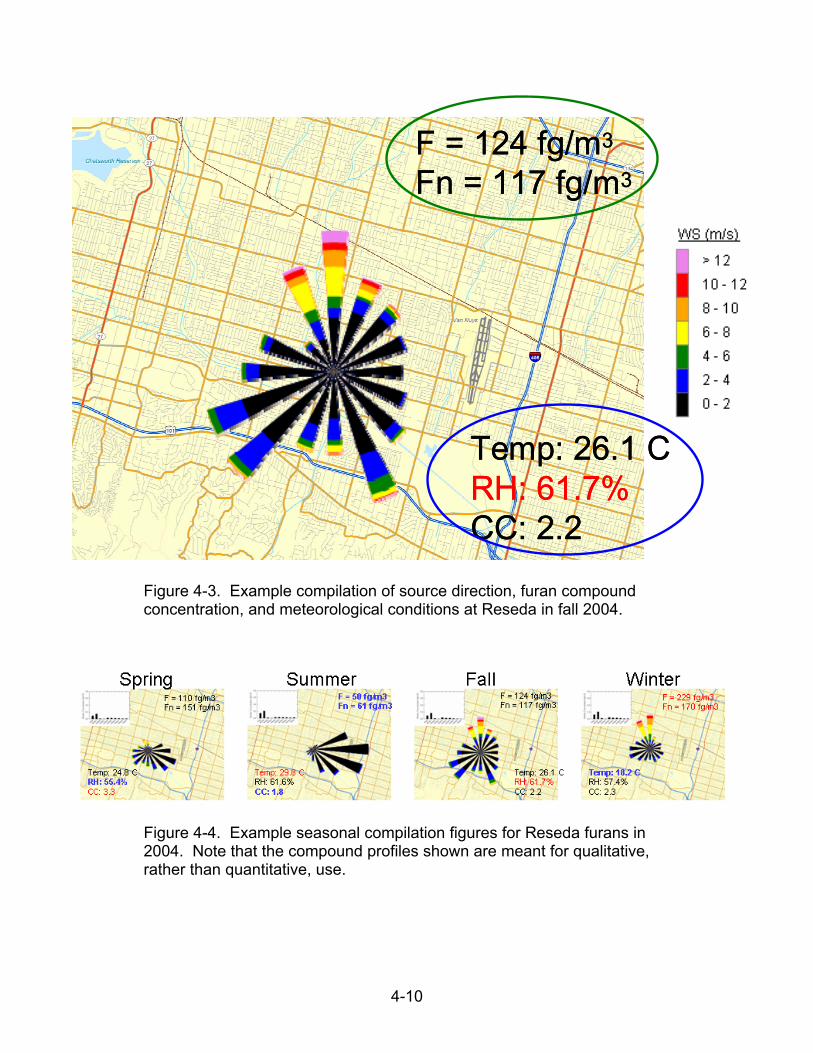
4-10

F = 124 fg/m3

Fn = 117 fg/m3

F = 124 fg/m3

Fn = 117 fg/m3

Temp: 26.1 C RH: 61.7%CC: 2.2

Temp: 26.1 C RH: 61.7%CC: 2.2

Figure 4-3. Example compilation of source direction, furan compound concentration, and meteorological conditions at Reseda in fall 2004.

Figure 4-4. Example seasonal compilation figures for Reseda furans in 2004. Note that the compound profiles shown are meant for qualitative, rather than quantitative, use.

4-11

4.2 RESULTS

The meteorological analysis was based on individual regression, time series, multiple-linear regression, and source analysis. Because the sampling frequency of the dioxins, furans, and biphenyls limited the nature of these analyses, it was difficult to fully understand the cause and effect relationship between dioxins, furans, and biphenyls and meteorology. However, these analyses show that the spatial and temporal variations of meteorology and dioxin, furan, and biphenyl concentrations are often related. Some of the analyses are sound enough to support conclusions about the causes of the relationship, while others show that data are at least consistent with hypotheses that could be further tested with future analyses and measurement programs.

4.2.1 Individual Regression Analysis Results

Table 4-4 lists correlation coefficients between selected meteorological parameters and dioxins, furans, and biphenyls for Sacramento. Correlation matrices for all sites are provided in accompanying material. In general, the correlation coefficients among dioxins, furans, and biphenyls and meteorology were directionally similar, but generally higher for Sacramento compared to other areas. In addition, some variables, such as relative humidity, had a good relationship with dioxins, furans, and biphenyls for Sacramento, but poor relationships in other areas. Because the number of observations was small, the correlations between the individual meteorological parameters and compound concentrations should be viewed with caution.

Table 4-4. Correlation coefficients (R2) for Sacramento. Positive correlations are shaded red. Bold correlation coefficients indicate the highest correlation for each compound.

Meteorological Parameter Biphenyls Dioxin Furans 925 mb Temperature 0.44 0.39 0.40 Maximum Temperature 0.24 0.52 0.66 Average Morning Temperature Maximum Mixing Height

0.24 0.00

0.55 0.47

0.68 0.71

Ventilation Index 0.00 0.33 0.50 West to East Transport 0.00 0.35 0.78 Average RH 0.31 0.52 0.70

Overall, furans and dioxins show a similar relationship with meteorology and are negatively correlated with all parameters except RH. Biphenyls behave quite differently and are positively correlated with all meteorological parameters except RH.

Dioxins

Non-adjusted for ventilation: Dioxins have high correlation coefficients and, like furans, are negatively correlated with temperature, mixing height, west-to-east transport, and ventilation, and positively correlated with RH. Dioxin concentrations are high when

4-12

temperatures are cold, mixing is limited, RH is high, and ventilation is poor—conditions that generally occur in the winter.

Adjusted for ventilation: When dioxin concentrations are adjusted for ventilation, the relationship with RH and temperature disappears, indicating that dioxin concentrations are most influenced by ventilation.

Furans

Non-adjusted for ventilation: Furans have very high correlation coefficients and are negatively correlated with temperature, mixing height, transport, and ventilation. Furan concentrations are high when temperatures are cold, mixing is limited, RH is high (a positive correlation), and ventilation is poor—conditions that generally occur in the winter.

Adjusted for ventilation: When concentrations are adjusted to remove the influence of ventilation, the negative relationship with temperature turns positive and the relationship with RH turns negative, indicating that furan concentrations, like dioxins, are most influenced by ventilation and not temperature or RH.

Biphenyls

Non-adjusted for ventilation: Biphenyls have a positive correlation with temperature and negative correlation with RH, but have no relationship with mixing height or ventilation. High biphenyl concentrations occur when it is warm and dry. Because warm and dry conditions generally occur in the summer when ventilation is high, the influence of temperature actually overwhelms the influence of increased ventilation that occurs during the summer.

Adjusted for ventilation: When adjusted for ventilation, the positive relationship between temperature and biphenyls is enhanced as is the negative relationship with RH. Because biphenyl concentrations are known to increase due to volatilization (Baird and Cann, 2005), we suggest that the high warm season concentrations are due to high temperatures and not low RH. RH is directly influenced by temperature, and RH’s relationship with biphenyls is likely an artifact of that effect.

4.2.2 Time Series Results

Figures 4-5 through 4-7 show time series plots of ventilation-adjusted dioxins, furans, and biphenyls and maximum temperature, respectively, for Boyle Heights (BH), Crocket (CRO), Livermore (LIV), Reseda (RES), Rubidoux (RUB), and Sacramento (SAC). Time series plots for the other meteorological variables are provided in accompanying material.

Dioxins

Ventilation-adjusted dioxin concentrations show no relationship with maximum temperature at all sites except Rubidoux. A very weak positive relationship with temperature indicates that when temperatures increase, so do dioxin concentrations at

4-13

12/2001

6/2002

12/2002

6/2003

12/2003

6/2004

12/2004

6/2005

12/2005

6/2006

0

1

2

3

4

5N

orm

aliz

ed C

once

ntra

tion

12/2001

4/2002

8/2002

12/2002

4/2003

8/2003

12/2003

4/2004

8/2004

12/2004

0

1

2

3

4

5

Nor

mal

ized

Con

cent

ratio

n

LIV

RES

SAC

2/2003

4/2003

6/2003

8/2003

10/2003

12/2003

2/2004

4/2004

6/2004

8/2004

10/2004

12/2004

0

1

2

3

4

5

12/2001

6/2002

12/2002

6/2003

12/2003

6/2004

12/2004

6/2005

12/2005

6/2006

0

1

2

3

4

5

Nor

mal

ized

Con

cent

ratio

n

RUB12/2001

4/2002

8/2002

12/2002

4/2003

8/2003

12/2003

4/2004

8/2004

12/2004

0

1

2

3

4

5

Nor

mal

ized

Con

cent

ratio

n

CRO

BH

12/2001

4/2002

8/2002

12/2002

4/2003

8/2003

12/2003

4/2004

8/2004

12/2004

0

1

2

3

4

5

Nor

mal

ized

Con

cent

ratio

n

Dioxin Concentration Maximum Temperature

12/2001

6/2002

12/2002

6/2003

12/2003

6/2004

12/2004

6/2005

12/2005

6/2006

0

1

2

3

4

5N

orm

aliz

ed C

once

ntra

tion

12/2001

4/2002

8/2002

12/2002

4/2003

8/2003

12/2003

4/2004

8/2004

12/2004

0

1

2

3

4

5

Nor

mal

ized

Con

cent

ratio

n

LIV

RES

SAC

2/2003

4/2003

6/2003

8/2003

10/2003

12/2003

2/2004

4/2004

6/2004

8/2004

10/2004

12/2004

0

1

2

3

4

5

12/2001

6/2002

12/2002

6/2003

12/2003

6/2004

12/2004

6/2005

12/2005

6/2006

0

1

2

3

4

5

Nor

mal

ized

Con

cent

ratio

n

RUB12/2001

4/2002

8/2002

12/2002

4/2003

8/2003

12/2003

4/2004

8/2004

12/2004

0

1

2

3

4

5

Nor

mal

ized

Con

cent

ratio

n

CRO

BH

12/2001

4/2002

8/2002

12/2002

4/2003

8/2003

12/2003

4/2004

8/2004

12/2004

0

1

2

3

4

5

Nor

mal

ized

Con

cent

ratio

n

Dioxin Concentration Maximum Temperature

LIV

RES

SAC

2/2003

4/2003

6/2003

8/2003

10/2003

12/2003

2/2004

4/2004

6/2004

8/2004

10/2004

12/2004

0

1

2

3

4

5

12/2001

6/2002

12/2002

6/2003

12/2003

6/2004

12/2004

6/2005

12/2005

6/2006

0

1

2

3

4

5

Nor

mal

ized

Con

cent

ratio

n

RUB12/2001

4/2002

8/2002

12/2002

4/2003

8/2003

12/2003

4/2004

8/2004

12/2004

0

1

2

3

4

5

Nor

mal

ized

Con

cent

ratio

n

CRO

BH

12/2001

4/2002

8/2002

12/2002

4/2003

8/2003

12/2003

4/2004

8/2004

12/2004

0

1

2

3

4

5

Nor

mal

ized

Con

cent

ratio

n

Dioxin ConcentrationDioxin Concentration Maximum TemperatureMaximum Temperature

Figure 4-5. Time series plots of normalized, ventilation-adjusted dioxin concentrations and maximum temperature at six sites.

4-14

LIV

12/2001

6/2002

12/2002

6/2003

12/2003

6/2004

12/2004

6/2005

12/2005

6/2006

0

1

2

3

4

5

Nor

mal

i zed

Con

cent

rat io

n

RES

12/2001

4/2002

8/2002

12/2002

4/2003

8/2003

12/2003

4/2004

8/2004

12/2004

0

1

2

3

4

5

Nor

mal

i ze

d C

once

ntr

atio

n

SAC

2/2003

4/2003

6/2003

8/2003

10/2003

12/2003

2/2004

4/2004

6/2004

8/2004

10/2004

12/2004

0

1

2

3

4

5

RUB

12/2001

6/2002

12/2002

6/2003

12/2003

6/2004

12/2004

6/2005

12/2005

6/2006

0

1

2

3

4

5

Nor

mal

ized

Con

cent

rat io

n

CRO

12/2001

4/2002

8/2002

12/2002

4/2003

8/2003

12/2003

4/2004

8/2004

12/2004

0

1

2

3

4

5

Nor

mal

ized

Con

cent

rat io

n

BH

12/2001

4/2002

8/2002

12/2002

4/2003

8/2003

12/2003

4/2004

8/2004

12/2004

0

1

2

3

4

5

Nor

mal

ized

Con

cent

rat io

n

Furan Concentration Maximum Temperature

LIV

12/2001

6/2002

12/2002

6/2003

12/2003

6/2004

12/2004

6/2005

12/2005

6/2006

0

1

2

3

4

5

Nor

mal

i zed

Con

cent

rat io

n

LIV

12/2001

6/2002

12/2002

6/2003

12/2003

6/2004

12/2004

6/2005

12/2005

6/2006

0

1

2

3

4

5

Nor

mal

i zed

Con

cent

rat io

n

RES

12/2001

4/2002

8/2002

12/2002

4/2003

8/2003

12/2003

4/2004

8/2004

12/2004

0

1

2

3

4

5

Nor

mal

i ze

d C

once

ntr

atio

n

RES

12/2001

4/2002

8/2002

12/2002

4/2003

8/2003

12/2003

4/2004

8/2004

12/2004

0

1

2

3

4

5

Nor

mal

i ze

d C

once

ntr

atio

n

SAC

2/2003

4/2003

6/2003

8/2003

10/2003

12/2003

2/2004

4/2004

6/2004

8/2004

10/2004

12/2004

0

1

2

3

4

5SAC

2/2003

4/2003

6/2003

8/2003

10/2003

12/2003

2/2004

4/2004

6/2004

8/2004

10/2004

12/2004

0

1

2

3

4

5

RUB

12/2001

6/2002

12/2002

6/2003

12/2003

6/2004

12/2004

6/2005

12/2005

6/2006

0

1

2

3

4

5

Nor

mal

ized

Con

cent

rat io

n

RUB

12/2001

6/2002

12/2002

6/2003

12/2003

6/2004

12/2004

6/2005

12/2005

6/2006

0

1

2

3

4

5

Nor

mal

ized

Con

cent

rat io

n

CRO

12/2001

4/2002

8/2002

12/2002

4/2003

8/2003

12/2003

4/2004

8/2004

12/2004

0

1

2

3

4

5

Nor

mal

ized

Con

cent

rat io

n

CRO

12/2001

4/2002

8/2002

12/2002

4/2003

8/2003

12/2003

4/2004

8/2004

12/2004

0

1

2

3

4

5

Nor

mal

ized

Con

cent

rat io

n

BH

12/2001

4/2002

8/2002

12/2002

4/2003

8/2003

12/2003

4/2004

8/2004

12/2004

0

1

2

3

4

5

Nor

mal

ized

Con

cent

rat io

n

BH

12/2001

4/2002

8/2002

12/2002

4/2003

8/2003

12/2003

4/2004

8/2004

12/2004

0

1

2

3

4

5

Nor

mal

ized

Con

cent

rat io

n

Furan ConcentrationFuran Concentration Maximum TemperatureMaximum Temperature

Figure 4-6. Time series plots of normalized, ventilation-adjusted furans concentrations and maximum temperature at six sites.

4-15

12/2001

6/2002

12/2002

6/2003

12/2003

6/2004

12/2004

6/2005

12/2005

6/2006

0

1

2

3

4

5

No

rma

lized

Con

cen

trat

ion

LIV

12/2001

4/2002

8/2002

12/2002

4/2003

8/2003

12/2003

4/2004

8/2004

12/2004

0

1

2

3

4

5

Nor

mal

ize

d C

onc

entr

atio

n

RES2/2003

4/2003

6/2003

8/2003

10/2003

12/2003

2/2004

4/2004

6/2004

8/2004

10/2004

12/2004

0

1

2

3

4

5

Nor

mal

ize

d C

o nce

ntra

tion

SAC

12/2001

6/2002

12/2002

6/2003

12/2003

6/2004

12/2004

6/2005

12/2005

6/2006

0

1

2

3

4

5

Nor

mal

ize

d C

onc

entr

atio

n

RUB12/2001

4/2002

8/2002

12/2002

4/2003

8/2003

12/2003

4/2004

8/2004

12/2004

0

1

2

3

4

5

Nor

mal

ize

d C

onc

entr

atio

n

CRO

12/2001

4/2002

8/2002

12/2002

4/2003

8/2003

12/2003

4/2004

8/2004

12/2004

0

1

2

3

4

5

Nor

mal

ize

d C

onc

entr

atio

n

BH

Biphenyl Concentration Maximum Temperature

12/2001

6/2002

12/2002

6/2003

12/2003

6/2004

12/2004

6/2005

12/2005

6/2006

0

1

2

3

4

5

No

rma

lized

Con

cen

trat

ion

LIV

12/2001

4/2002

8/2002

12/2002

4/2003

8/2003

12/2003

4/2004

8/2004

12/2004

0

1

2

3

4

5

Nor

mal

ize

d C

onc

entr

atio

n

RES2/2003

4/2003

6/2003

8/2003

10/2003

12/2003

2/2004

4/2004

6/2004

8/2004

10/2004

12/2004

0

1

2

3

4

5

Nor

mal

ize

d C

o nce

ntra

tion

SAC

12/2001

6/2002

12/2002

6/2003

12/2003

6/2004

12/2004

6/2005

12/2005

6/2006

0

1

2

3

4

5

Nor

mal

ize

d C

onc

entr

atio

n

RUB12/2001

4/2002

8/2002

12/2002

4/2003

8/2003

12/2003

4/2004

8/2004

12/2004

0

1

2

3

4

5

Nor

mal

ize

d C

onc

entr

atio

n

CRO

12/2001

4/2002

8/2002

12/2002

4/2003

8/2003

12/2003

4/2004

8/2004

12/2004

0

1

2

3

4

5

Nor

mal

ize

d C

onc

entr

atio

n

BH

Biphenyl ConcentrationBiphenyl Concentration Maximum TemperatureMaximum Temperature

Figure 4-7. Time series plots of normalized, ventilation-adjusted biphenyl concentrations and maximum temperature at six sites.

4-16

Rubidoux. It is not clear from this limited analysis if the relationship is due to temperature directly affecting dioxin concentrations, an artifact of the ventilation adjustment, or seasonal changes in emissions that impact the site.

The correlation analysis for Sacramento showed that prior to adjusting for ventilation, dioxins correlated negatively with maximum temperature. However, after adjusting for ventilation, the time series of dioxin concentrations shows no clear relationship with maximum temperature or any of the other meteorological parameters. This illustrates the importance of adjusting the data for ventilation to properly assess the influence of other meteorological parameters or seasonal sources on pollutant concentrations.

Furans

The adjusted concentrations for Sacramento, Crocket, and Rubidoux show a seasonal cycle with high concentrations in the summertime and low concentrations in the wintertime (note that this is opposite non-adjusted concentrations). Thus, any meteorological parameter that exhibits a strong seasonal cycle has a good relationship with furan concentrations. These meteorological parameters include maximum temperature, aloft temperature, mixing height, and precipitation. However, it is not clear from this analysis which of these variables cause the seasonal cycle of ventilation-adjusted furan concentrations. What is clear is that ventilation has an important impact on furan concentrations. For example, the ventilation adjustment concentrations for Sacramento are eight times lower in the wintertime and one-third higher in the summertime compared to the non-adjusted concentrations.

For Rubidoux and Crocket, the adjusted furan concentrations show the best relationships with 850 mb temperature. These positive relationships probably indicate how well 850-mb temperature varies by season, rather than indicating a direct impact of 850-mb temperature on furan concentrations.

For Boyle Heights, Livermore, and Reseda, there is no clear seasonal pattern in ventilation-adjusted furan concentrations and no clear relationship with any of the meteorological parameters. This lack of relationship is similar to the dioxin findings.

Biphenyls

Adjusted biphenyl concentrations show a strong seasonal relationship at all sites. During the summertime adjusted concentrations are high and during the wintertime they are low. Thus, any meteorological parameter that exhibits a strong seasonal cycle shows a good relationship with biphenyl concentrations, including maximum temperature. That adjusted biphenyl concentrations remain high in the summertime despite high ventilation indicates that biphenyls are strongly influenced by processes other than ventilation. That biphenyls increase at all sites in the summertime suggests that the increase has less to do with seasonal changes in the transport of emissions from nearby sources, and more to do with temperature changes, which influence all sites in California in a similar fashion over the year.

4-17

4.2.3 Multiple-linear Regression Results

Multiple-linear regression analyses were performed on the non-ventilation adjusted concentrations prior to the time series and individual regression analyses. However, as the time series and individual regression analyses demonstrated, adjusting for ventilation is a key to understanding the relationship between dioxins, furans, biphenyls, and diphenylethers and meteorology. In addition, to provide an adequate number of samples for robust regression calculations, all available data were included in the regression analysis (i.e., data were not partitioned spatially). Combining the data was a necessary step in this exploration; however, interpretation of results was further complicated. Because of these issues, only a brief summary of our findings from the regression analysis is provided. A more detailed discussion can be found in Appendix B.

The total variance in dioxin concentrations explained by meteorology is 39 percent. To provide context, in our experience in California, meteorology typically explains about 50 to 60 percent of variance of daily 24-hr PM2.5 concentrations and 60 to 75 percent of the variance of daily maximum 8-hr ozone concentrations. Therefore, 39 percent is a fair correlation given the limited data set and the large spatial area covered by the samples.

The total variance in furan concentrations explained by meteorology is 68 percent. This correlation is high for meteorology and air quality parameters and is on par with correlation coefficients for meteorology and daily ozone concentrations.

The total variance in biphenyl concentrations explained by meteorology is 44 percent. Like dioxins, this correlation is fair, given the limited data set and the large spatial area covered by the samples.

4.2.4 Source Analysis Results

To determine the influence of source area, compilation plots were generated for Sacramento, Reseda, and Rubidoux for each season and year. The compilation plots contain wind roses, fingerprints of compound groups, ventilation-adjusted and non-adjusted compound group concentrations, and seasonal averages of the daily average RH, daily average cloud coverage, and daily maximum temperature. The findings are presented by site.

Figures 4-8 through 4-10 show the Sacramento compilation plots for dioxins, furans, and biphenyls. The following observations are noted:

Seasonal Wind Patterns. Winds during all seasons in 2003 and 2004 were predominately from the southern quadrant. In the winter, strong winds were more often from the southeast, and in the fall they were more often from the southwest. Storm systems cause the strong winter southeast winds. In the spring, the strong winds are due to storm systems and the Delta breeze. In all seasons except summer, winds came from the west and northwest, due to clearing winds behind storms. Strong winds never came from the northeast or

4-18

east. Light winds were most common in the fall and winter and least common in the summer. These slow wind speeds, along with low mixing heights, contribute to low ventilation observed in the winter.

Yearly Wind Differences. Wind patterns differ little between years. There are a few notable exceptions:

– Westerly winds occurred more frequently in winter 2003 compared to those in winter 2004.

– Strong northwesterly winds occurred more frequently and westerly and southwesterly winds less frequently in fall 2004 compared to those in fall 2003

– More periods of stronger winds occurred in spring 2004 compared to those in spring 2003.

Possible Sources. Because the wind patterns were generally similar between years, it is difficult to determine if specific upwind source areas explain the yearly differences in concentrations. That being said, we offer the following observations:

– Ventilation-adjusted dioxin concentrations were about 50 percent lower in spring 2004 compared to spring 2003. Winds were more often from the northwest in 2004 and less often from the south compared to 2003. This pattern suggests that there are more sources of dioxins south of the measurement site than northwest. It should also be noted that spring maximum temperatures were on average much warmer in 2004 compared to 2003; however, based on previous analyses, it is unlikely that temperature is the cause of this difference in dioxin concentrations.

– Yearly differences in furan concentrations by season are similar to those of dioxins (with the exception of spring), indicating that furans have source areas similar to those of dioxins in Sacramento. Furan concentrations were similar in springs 2003 and 2004 while dioxins were twice as high in spring 2003 compared to spring 2004. There is no clear explanation for this difference.

– During most seasons, biphenyls behaved differently than the dioxins and furans. In the spring, biphenyl concentrations are significantly lower in 2003 compared to 2004, whereas, dioxin and furan concentrations were higher. Of note, spring 2004 was much warmer than spring 2003, which likely led to higher biphenyl concentrations.

– In the winter, when temperatures were about the same between years, adjusted biphenyl concentrations were more than five times higher in 2004 compared to 2003, suggesting that biphenyl concentrations are affected by factors other than temperature.

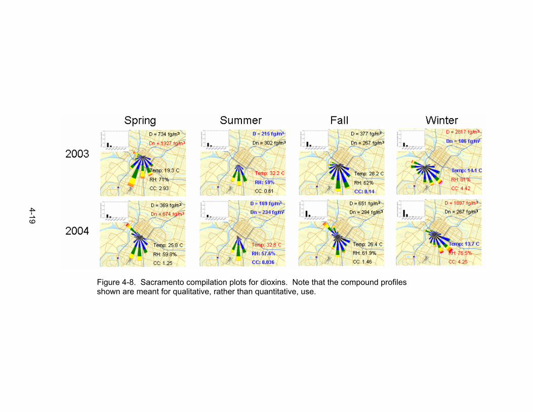
4-19

Figure 4-8. Sacramento compilation plots for dioxins. Note that the compound profiles shown are meant for qualitative, rather than quantitative, use.

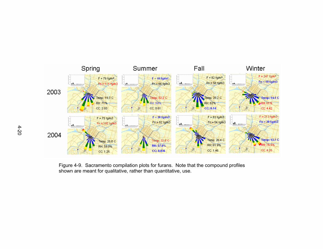
4-20

Figure 4-9. Sacramento compilation plots for furans. Note that the compound profiles shown are meant for qualitative, rather than quantitative, use.

4-21

Figure 4-10. Sacramento compilation plots for biphenyls. Note that the compound profiles shown are meant for qualitative, rather than quantitative, use.

4-22

Figures 4-11 through 4-13 show the Reseda compilation plots for dioxins, furans, and biphenyls. The following observations are noted.

Seasonal Wind Patterns. Compared to Sacramento, wind directions in 2002-2004 were much more evenly distributed during spring, fall, and winter. In the summer, winds were predominantly from the northeast to southeast and were generally light. In the spring, winter, and fall, there were periods of strong winds from the northerly quadrant. The strong northerly winds were likely Santa Ana winds and post-frontal clearing winds.

Yearly Wind Differences. Wind patterns differ little between years with the exception more frequent stronger northerly and southerly winds in fall 2004.

Possible Sources. Because wind patterns were generally similar between years, it is difficult to determine if specific upwind source areas explain the yearly differences in concentrations. That being said, we offer the following observations.

– Ventilation-adjusted and non-adjusted dioxin concentrations were about 50 percent or more higher in spring 2002 compared to spring 2003 and 2004. This difference cannot be explained by transport. However, 2002 was cloudier and cooler than 2003 and 2004. It has been suggested that OH radicals may be a significant sink for dioxins and furans. A cloudier spring in 2002 may have caused a reduction in available OH radicals at the surface, thus an increase in dioxin and furan concentrations.

– Ventilation-adjusted dioxin concentrations were about 300 to 400 percent higher in fall 2002 compared to fall 2003 and 2004. This seasonal average concentration is influenced by a single, large concentration spike in fall 2002 (Figure 4-5 [RES]). This spike in concentrations cannot be explained by transport differences but is mirrored by the furan concentrations (Figure 4-6 [RES]), perhaps indicating an unusual emissions event.

– Ventilation-adjusted dioxin concentrations were about 35 percent greater in fall 2004 than fall 2003. In 2004, more periods of strong northerly and southerly winds occurred.

– During fall 2002, ventilation-adjusted furan concentrations were about five times greater than in fall 2003 and 2004. Dioxin and furan concentrations may both be strongly influenced by the same unusual emission source in 2002. Like dioxins, ventilation-adjusted furans were also greater in 2004, when northerly winds were more frequent compared to 2003.

– Unlike furans and dioxins, ventilation-adjusted biphenyl concentrations were similar in fall 2002 and 2003, indicating that whatever caused the high furan and dioxin concentrations in 2002 may not have had the same impact on biphenyls.

– In fall 2004, biphenyls were much lower than in fall 2003, probably because temperatures were lower in fall 2004.

4-23

– Ventilation-adjusted and non-adjusted biphenyl concentrations are much lower in summer 2004 compared to summer 2002 and 2003. The reason is not clear, given similar temperatures and transport patterns among the years.

Figures 4-14 through 4-16 show the Rubidoux compilation plots for dioxins, furans, and biphenyls. The following observations are noted.

Seasonal Wind Patterns. Spring, summer, and fall 2002-2005 were dominated by westerly winds. Periods of strong winds from the northerly quadrant occurred in fall. Winter wind directions were roughly evenly distributed, but most commonly came from the northerly quadrant. Strong winds occurred year-round and were typically from the west or north. The strong northerly winds in the fall, winter, and spring were likely Santa Ana winds and post-frontal clearing winds. Westerly winds are caused by the sea breeze.

Yearly Wind Differences. There is virtually no difference in the wind patterns among years.

Possible Sources: Because the wind patterns were so similar among years, it is not possible to determine if specific upwind source areas explain the yearly differences in concentrations. That being said, we offer the following observations.

– Spring ventilation-adjusted and non-adjusted dioxin concentrations were much higher in 2005 compared to the other years, despite similar meteorology and transport patterns. An unusual emission event may have occurred in 2005 that impacted dioxins measured at Rubidoux. Furans did not exhibit this marked increase in 2005, which means that whatever caused the high dioxin concentrations did not influence furans to the same degree.

– Summer ventilation-adjusted and non-adjusted dioxins concentrations were much higher in 2004 compared to the other years despite similar meteorology and transport patterns. This finding suggests that an unusual emission event occurred. Furans do not exhibit this marked increase in 2004, which means that whatever caused the high dioxin concentrations did not influence furans to the same degree.

– Fall ventilation-adjusted and non-adjusted dioxin concentrations were higher in 2002 compared to the other years. Fall 2002 was much cooler and cloudier than other years. An increase in dioxin concentrations under cooler and cloudier conditions was also observed at Reseda during summer 2003.

– Winter ventilation-adjusted dioxin concentrations were significantly higher in 2002 despite similar meteorological and transport patterns. The cause of the higher concentrations is not clear.

– For all seasons, biphenyl concentrations were highest during periods of highest temperatures—which occurred in summers 2002-2005, spring 2004, and fall 2003.

4-24

Figure 4-11. Reseda compilation plots for dioxins. Note that the compound profiles shown are meant for qualitative, rather than quantitative, use.

4-25

Figure 4-12. Reseda compilation plots for furans. Note that the compound profiles shown are meant for qualitative, rather than quantitative, use.

4-26

Figure 4-13. Reseda compilation plots for biphenyls. Note that the compound profiles shown are meant for qualitative, rather than quantitative, use.

4-27

Figure 4-14. Rubidoux compilation plots for dioxins. Note that the compound profiles shown are meant for qualitative, rather than quantitative, use.

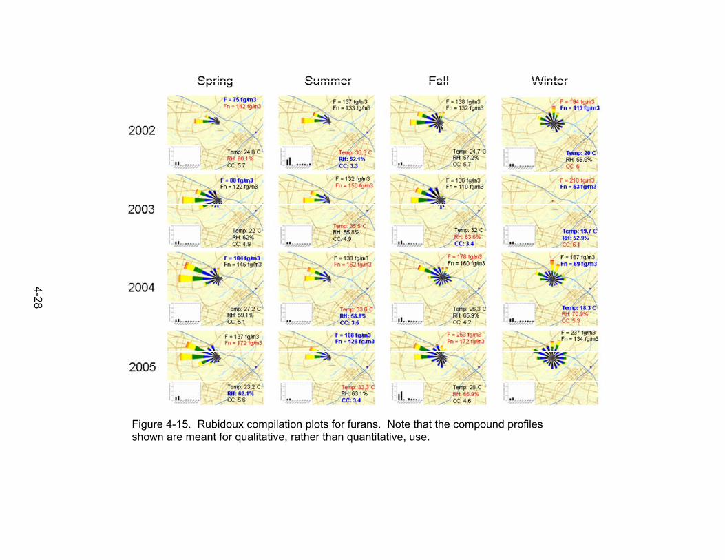
4-28

Figure 4-15. Rubidoux compilation plots for furans. Note that the compound profiles shown are meant for qualitative, rather than quantitative, use.

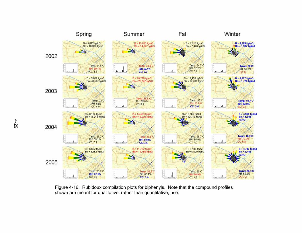
4-29

Figure 4-16. Rubidoux compilation plots for biphenyls. Note that the compound profiles shown are meant for qualitative, rather than quantitative, use.

4-30

4.3 METEOROLOGICAL ANALYSIS SUMMARY

Meteorological and air quality analyses were conducted to determine the relationship between meteorological conditions and the dioxins, furans, and biphenyls and their source regions:

Multi-linear regression analysis between dioxins, furans, and biphenyls and meteorological parameters to determine which meteorological parameters explain the most variance. Multiple-linear regression analyses were performed on the non-ventilation adjusted concentrations. However, as subsequent analyses demonstrated, adjusting for ventilation (see bullet 3) is vital to understanding the relationship between dioxins, furans, and biphenyls and meteorology not influenced by ventilation (i.e., temperature, relative humidity, wind direction, etc). In addition, to provide an adequate number of samples for robust regression calculations, data from all sites were included in the regression analysis. It was difficult to draw conclusions from the multiple-linear regression results.

Individual linear regression analysis between dioxins, furans, and biphenyls and the meteorological parameters for each site. This analysis proved more useful than multiple-linear regression and offered insight into the relationship between meteorology and dioxins, furans, and biphenyls . This analysis was especially useful when coupled with subjective analysis of time series plots (see bullet 4).

Adjustments to remove the effect of ventilation on concentrations. Low ventilation in cool months can cause high pollutant concentrations, while higher ventilation in warm months can cause low concentrations. Concentrations were adjusted for ventilation to remove this effect. Ventilation is a measure of the volume of the air into which pollutants disperse and is calculated by multiplying wind speed and mixing height. Although the mixing height and wind data used in the analysis contain some degree of uncertainty, accounting for the effect of ventilation was important to elucidate the relationship between non-ventilation processes (meteorological and emission sources) and dioxin, furan, and biphenyl concentrations.

Subjective analysis of time series plots of the ventilation-adjusted dioxin, furan, and biphenyl, concentrations and meteorological parameters that explain the most variance. The meteorological parameters investigated were maximum surface temperature, aloft temperature, mixing height, relative humidity, and precipitation. The time series analysis coupled with the regression analysis provided good insight into how meteorology influences dioxin, furan, and biphenyl concentrations.

Subjective analysis of wind roses, compound fingerprints and average concentrations, mixing height normalized concentrations, and weather conditions by site, season, and year to determine whether a relationship exists between source areas and dioxins, furans, and biphenyls. This analysis provided some insight into potential source areas of high concentrations of dioxins, furans, and biphenyls. It also showed that the combined influence of meteorology and transport on concentrations of dioxins, furans, and biphenyls is complex and

4-31

requires detailed case study analysis beyond that performed in this exploratory work.

Highlights of Findings

Dioxins

Dioxins are negatively correlated with ventilation.

Ventilation-adjusted dioxin concentrations show no significant seasonal pattern. This illustrates the importance of adjusting the data for ventilation to properly assess the influence of other meteorological parameters on pollutant concentrations.

At Reseda, ventilation-adjusted dioxin concentrations were about 50 percent higher in spring 2002 compared to spring 2003 and 2004. This difference cannot be explained by transport. It was cloudier and cooler in 2002 than in 2003 and 2004. It has been suggested that OH radicals may be a significant sink for dioxins and furans. A cloudier spring in 2002 may have caused a reduction in available OH radicals at the surface, thus an increase in dioxin and furan concentrations.

Furans

Furan concentrations are negatively correlated with ventilation.

Ventilation has an important impact on furan concentrations. For example, the ventilation-adjusted concentrations at Sacramento are eight times lower in the wintertime and one-third higher in the summertime compared to the non-adjusted concentrations.

The ventilation adjustments account for most of the seasonal patterns.

At Sacramento, yearly differences in furan concentrations by season are similar to those of dioxins, indicating that furans have source areas similar to those of dioxins.

Biphenyls

Biphenyl concentrations are positively correlated with ventilation.

Ventilation-adjusted biphenyl concentrations are high during the summertime and low during the wintertime at all sites. When adjusted for ventilation, summer biphenyl concentrations are still higher than in other seasons. Based on correlations (Table 4-4), temperature may account for this behavior (i.e., increased volatilization with increased temperature).

At Rubidoux, for all seasons, biphenyl concentrations were highest during periods of highest temperatures—which occurred in spring 2004, summer and fall 2003, and winter 2005.

That biphenyl concentrations increase at all sites in the summertime suggests that the increase is less influenced by seasonal changes in the transport of emissions from nearby sources, and influenced more by temperature changes, which similarly influence all sites in California over the year. However, it should

4-32

be noted that at Sacramento in the winter, when temperatures were about the same between years, adjusted biphenyl concentrations were higher in 2004 compared to 2003, suggesting that biphenyl concentrations were affected by factors other than temperature.

At Reseda, unlike furans and dioxins, ventilation-adjusted biphenyl concentrations were similar in fall 2002 and 2003, indicating that whatever caused the high furan and dioxin concentrations in 2002 did not have the same impact on biphenyls.

5-1

5. SOURCE APPORTIONMENT AND CASE STUDY ANALYSIS

5.1 TECHNICAL APPROACH

The use of three statistical tools was explored to attempt to understand, and potentially quantify, emission sources contributing to dioxin, furan, biphenyl, and diphenylether concentrations: principal component analysis (PCA), chemical mass balance (CMB), and positive matrix factorization (PMF).

5.1.1 Principal Component Analysis (PCA)

Principal component analysis (PCA) was conducted to identify sources of dioxins, furans, and biphenyls. PCA identifies groups of species that covary. The covariance is typically due to common emissions sources (e.g., vehicle exhaust) or atmospheric processing such as deposition, dilution, or formation (e.g., sulfate formation from SO2). PCA is a common type of factor analysis applied to atmospheric data and has been used extensively on a wide variety of data sets (for example, Pancras et al., 2006; García et al., 2006; Ho et al., 2006). The method used in this analysis is known as variance maximizing (varimax) rotation. Essentially, the original variable space is rotated so that the variance around the new axes is maximized. This gives the most variance within each factor, enabling easier interpretation. PCA extracts factors so that the first factor explains the most variability in a data set and consecutive factors explain relatively less and less variance. The goal is to maximize the amount of information about a data set (measured by the variance) while minimizing the number of factors. PCA uses Eigen analysis, in which variance of a new factor is expressed as that factor’s eigenvalue. In this analysis, only factors with eigenvalues greater than 1 were retained, a typical threshold for PCA. Sensitivity analysis was conducted using eigenvalues less than 1 to ensure that meaningful factors were not excluded.

5.1.2 Chemical Mass Balance (CMB)

CMB is a source apportionment method that solves a series of linear equations with a least squares solution in which each equation represents the concentration of a chemical species measured at the receptor as the sum of the products of source contributions and source profiles (Watson, 1979). For each species i, the concentration of i measured at the monitoring site is the sum of source contributions from source j (Sj) times the fraction of Sj composed of species i (Fij) for the number of sources (n) sources (Equation 5-1). To obtain a unique solution, the number of chemical species must be greater than n.

n

jiji SFC1

(5-1)

The required inputs for running CMB are an ambient data set and source profiles. The ambient data set includes concentrations measured at a monitoring site for each chemical species over time. Source profiles include the fractional contributions for each

5-2

chemical species emitted by a source to the total mass emitted by that source. Because source profiles are required input, sources must be identified and their emissions characterized prior to running the CMB model. It is important to use source profiles that are representative of local sources and to model chemical species that have minimal reactivity. Alternatively, if sources are close to the monitoring site, reaction times are minimized. The desired result in running CMB is to determine the source contribution for each source input into the model. Determined source contributions represent the ambient concentration that can be attributed to the associated source.

5.1.3 Positive Matrix Factorization (PMF)

PMF is a multivariate factor analysis tool that has been applied to a wide range of data, including 24-hr speciated PM2.5 data, size-resolved aerosol data, deposition data, air toxics data, and VOC data (Kim et al., 2003; Kim and Hopke, 2004; Brown et al., 2007; Lee et al., 2002; Kim et al., 2004; Pekney et al., 2006; Polissar et al., 2001; Ramadan et al., 2000; Poirot et al., 2001; Zhou et al., 2004; Zhao et al., 2004; Yakovleva et al., 1999; Song et al., 2001; Hwang and Hopke, 2006). Simply, PMF decomposes a matrix of ambient data into two matrices, which then need to be interpreted by the analyst as to what source types are represented. The method is described in detail elsewhere (Paatero, 1997; Paatero and Tapper, 1994).

The goal of multivariate receptor modeling such as PMF and CMB (Watson et al., 1990; Watson et al., 1991; Henry et al., 1984) is to identify a number of sources that best characterize the pollutant mix at a site, the species profile of each source, and the amount of mass contributed by each source to each individual sample. By individually weighing data, PMF allows days when data are missing or suspect to be retained, and the analyst can adjust the uncertainty so that these data also have a smaller impact on the final solution. The missing and below detection limit data are assigned much less weight compared with actual measured values, so these data are less important to the solution (Polissar et al., 2001; Hopke, 2003; Poirot et al., 2001; Ramadan et al., 2000; Lee et al., 2002; Song et al., 2001). In this analysis, data below the method detection limit (MDL) were substituted with half the maximum reported MDL. The maximum MDL was used for substitution because use of the sample-specific MDL could introduce a false source of variability in the data if there were regular changes in the sample-specific MDL. Missing data were substituted with median concentrations. Similar to previous studies (Polissar et al., 2001; Hopke, 2003; Poirot et al., 2001; Ramadan et al., 2000; Lee et al., 2002; Song et al., 2001), the uncertainty for data below detection was calculated as 5/6*MDL; and for missing data it was four times the median. A multi-linear regression of the factor contributions to the measured mass was then applied to provide scaling multipliers to normalize PMF results into the original mass units.

In this study, a standalone version of PMF (EPA PMF version 2.0) was used. EPA PMF is a graphical user interface that was based on the PMF model and solved using the multilinear engine as implemented in the program ME-2 (Paatero, 1999). EPA PMF operates in a robust mode, meaning that “outliers” are not allowed to overly influence the fitting of the contributions and profiles.

5-3

Model performance criteria are used to guide the final solution in PMF, including the goodness-of-fit parameter (Q) and convergence statistics. The final model output is also analyzed to determine how well the modeled results reproduce the input data. This includes examining the residuals for each species, the scatter plots between species, and the mass recovery.

Uncertainties in the EPA PMF solution are estimated using a bootstrapping technique, which is a re-sampling method in which “new” data sets are generated that are consistent with original data, each data set is decomposed into profile and contribution matrices, and the resulting profile and contribution matrices are compared with the base run (Eberly, 2005). Instead of inspecting point estimates, this method allows the analyst to review the confidence intervals for each species to obtain more robust profiles.

5.2 PRINCIPAL COMPONENT ANALYSIS RESULTS

PCA was run separately for each air basin to provide an adequate amount of data for the model. The resulting factors were similar across air basins and are thought to be influenced by similarities in seasonality of the respective compound groups as seen in other analyses. PCA results are shown in Table 5-1. For all air basins, the ten furans were in the same factor indicating that furans show very similar variability to each other. The biphenyls were also typically grouped together, with the exception of 3,3’,4,4’,5,5’-HxCB (HXCB1) in Sacramento (consistent with the correlation matrix depicted in Table 3-5). This species showed a seasonal pattern different from other biphenyls, which is likely the reason it was not grouped with the other biphenyls; because limited data are available, these results should not be over-interpreted. The diphenylethers were never all in the same group and were typically grouped by level of halogenation. That they were not grouped together indicates that the diphenylethers do not exhibit the same variability across levels of chlorination, which may be due to differences in vapor pressure. Additionally, diphenylethers were sometimes grouped with biphenyls. While this may indicate similar sources, the grouping is likely influenced by the similarity in seasonal patterns that were sometimes observed for furans and diphenylethers. The dioxins were in their own group in the South Coast Air Basin, but were divided in the other air basins; one group was associated with the furans. A similarity in sources of dioxins and furans may be indicated. While dioxins and furans are often emitted by similar sources, the results of this investigation are more likely explained by the similarity in seasonal pattern. The percent of total variance explained by each factor is also shown in Table 5-1. Biphenyls and diphenylethers contribute to the most variance in all air basins, while dioxins and furans contribute less variance.

5-4

Table 5-1. PCA results. Abbreviations are defined in Tables 2-1 through 2-4.

Factor Constituents

Percent of Variance Explained

Factor Constituents

Percent of Variance Explained

Factor Constituents

Percent of Variance Explained

Factor Constituents

Percent of Variance Explained

HXCB3 HXBDE5 PECB2 HXCDF2HXCB2 PEBDE3 PECB3 HPCDF1TETCB2 PEBDE1 HXCB4 HXCDF4HXCB4 HXBDE2 HXCB2 HXCDF3PECB2 TETBDE3 HXCB3 PECDF1PECB5 TETBDE2 HPCB2 HXCB1HPCB2 HXBDE1 TETCB2 HPCDF2HPCB3 HXBDE4 HPCB3 OCDFPECB3 PEBDE5 TRIBDE2 PECDF2PECB4 TETBDE6 TETBDE5 TETCDF

TETCB1 PEBDE2 TETBDE2 TETCDDPECB1 TETBDE4 DIBDE5 HXCDD2HPCB1 TETBDE5 TETBDE6 HXCDD1

TETBDE2 HXBDE3 DIBDE3 PECDDPEBDE2 TRIBDE2 PECDF1 HPCB3

TETBDE3 TRIBDE4 HXCDF4 HXCB2TRIBDE2 PECDF1 HXCDF3 HPCB2TETBDE5 HXCDF3 HXCDF2 HXCB3PEBDE1 HXCDF4 PECDF2 HXCB4

TETBDE6 HXCDF2 TETCDF PECB5HPCDF1 PECDF2 HPCDF1 PECB2HXCDF2 HPCDF1 HPCDF2 PECB3HXCDF3 HPCDF2 OCDF PECB4HXCDF4 OCDF PECDD TETCB2HPCDF2 TETCDF HXCDD2 PECB1PECDF1 HXCDD3 HXCDD1 HPCB1OCDF HXCDD2 HXBDE4 TETCB1

PECDF2 PECDD HXBDE2 OCDDHXCDF1 HXCDD1 PEBDE1 HXCDD3TETCDF PECB3 HXBDE1 HPCDD

NONBDE3 PECB2 HXBDE5NONBDE1 PECB4 TETBDE3NONBDE2 HXCB3 PEBDE2DECABDE HXCB2 PEBDE3PEBDE5 PECB5 PEBDE5HXBDE3 HXCB4 HXBDE3DIBDE3 TETCB2 TETBDE7DIBDE2 TETCB1 TETBDE4DIBDE4 PECB1 HPBDE1

TRIBDE1 HPCB3 OCDDDIBDE5 HPCB2 HPCDD

TRIBDE4 HPCB1 HXCDD3TETBDE4 DIBDE3 NONBDE1HXBDE1 DIBDE4 NONBDE2HXBDE2 DIBDE2 OBDEHXBDE5 TRIBDE1 NONBDE3PEBDE3 DIBDE5 DECABDEHXBDE4 NONBDE2 DIBDE2PECDD NONBDE1 DIBDE4

HXCDD3 NONBDE3HPCDD DECABDE

HXCDD1 OCDDHXCDD2 HPCDD

OCDD TETCDDTETCDD HPBDE1 4TETBDE1HPBDE1HPBDE2

DioxinsFuransBiphenylsDiphenyl Ethers

9

5

33

41

23

23

21

23

12

11

12

4

25

16

19

9

7

11

25

18

10

13

South Coast San Francisco Bay Area San Joaquin Valley Sacramento Valley

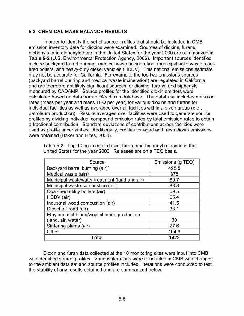
5-5

5.3 CHEMICAL MASS BALANCE RESULTS

In order to identify the set of source profiles that should be included in CMB, emission inventory data for dioxins were examined. Sources of dioxins, furans, biphenyls, and diphenylethers in the United States for the year 2000 are summarized in Table 5-2 (U.S. Environmental Protection Agency, 2006). Important sources identified include backyard barrel burning, medical waste incineration, municipal solid waste, coal-fired boilers, and heavy-duty diesel vehicles (HDDV). This national emissions estimate may not be accurate for California. For example, the top two emissions sources (backyard barrel burning and medical waste incineration) are regulated in California, and are therefore not likely significant sources for dioxins, furans, and biphenyls measured by CADAMP. Source profiles for the identified dioxin emitters were calculated based on data from EPA’s dioxin database. The database includes emission rates (mass per year and mass TEQ per year) for various dioxins and furans for individual facilities as well as averaged over all facilities within a given group (e.g., petroleum production). Results averaged over facilities were used to generate source profiles by dividing individual compound emission rates by total emission rates to obtain a fractional contribution. Standard deviations of contributions across facilities were used as profile uncertainties. Additionally, profiles for aged and fresh dioxin emissions were obtained (Baker and Hites, 2000).

Table 5-2. Top 10 sources of dioxin, furan, and biphenyl releases in the United States for the year 2000. Releases are on a TEQ basis.

Source Emissions (g TEQ) Backyard barrel burning (air)* 498.5 Medical waste (air)* 378 Municipal wastewater treatment (land and air) 89.7 Municipal waste combustion (air) 83.8 Coal-fired utility boilers (air) 69.5 HDDV (air) 65.4 Industrial wood combustion (air) 41.5 Diesel off-road (air) 33.1 Ethylene dichloride/vinyl chloride production (land, air, water) 30 Sintering plants (air) 27.6 Other 104.9

Total 1422

Dioxin and furan data collected at the 10 monitoring sites were input into CMB with identified source profiles. Various iterations were conducted in CMB with changes to the ambient data set and source profiles included. Iterations were conducted to test the stability of any results obtained and are summarized below.

5-6

1. Ambient data and source profiles in mass units were used versus TEQ units.

2. Compounds in the ambient data set and in profiles were combined by the number of halogens (e.g., dioxins with five chlorine atoms were combined) versus individual compounds.

3. Individual source profiles (e.g., medical waste incineration, diesel vehicles) were included versus averaged profiles (e.g., average of combustion sources, average of mobile sources).

4. The aged profile was added. The aged profile was only available on a mass basis and grouped by halide number; therefore, any iteration with this profile was conducted with ambient data and other profiles in mass units and grouped by chlorine number.

Results for the various CMB iterations are summarized in Table 5-3 for two sites, Rubidoux (RUB) and Livermore (LIV). The percent of the mass apportioned for each run is shown in the table as well as the sources to which mass was apportioned. The mass closure was poor for all runs conducted using ambient data and profiles in TEQ units, whereas approximately half the mass was apportioned when inputs were in mass units. The only source that was consistently implicated in all runs was motor vehicles. However, the percent of mass apportioned was not consistent between runs and, therefore, we cannot quantify the importance of mobile sources to ambient dioxin levels.

In general, CMB source apportionment with dioxin and furan data was not successful due to several limitations. Ambient samples are collected over a period of one month, providing significant time for reaction to occur. As a result, the relative abundance of the compounds in the atmosphere compared to what is seen in fresh emissions will change, making it difficult to apportion mass using this technique. In order to address this issue, the aged dioxin profile was included in several of the iterations. However, mass was not consistently apportioned to this source. Source profiles used in the analysis including the aged profile are not necessarily representative of local sources due to limited measurements of dioxin emissions. The lack of good source profiles restricts the ability of the model to apportion mass.

5.4 POSITIVE MATRIX FACTORIZATION RESULTS

PMF was run on three data sets: (1) a combined data set of data from all sites in California, (2) a Bay Area data set, and (3) a South Coast Air Basin data set. Overall, the results followed seasonal patterns and chlorination level.

The combined data set included data from Boyle Heights, Oakland, Reseda, Rubidoux, Sacramento, San Francisco, San Jose, and Wilmington. The sites used were “stacked”, meaning each site/date was considered a separate sample. Sites showing a much different distribution of data were removed from PMF analysis because they were consistently resolved into individual site factors as opposed to “source” factors. The final data set had 263 data points. Three to five factors were explored; only the three-factor solution was stable. The factors were divided by type, with a separate biphenyl, dioxin, and furan factor (see Figure 5-1).

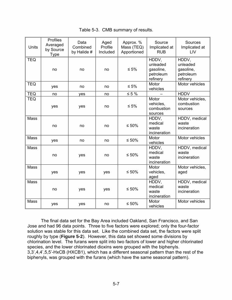
5-7

Table 5-3. CMB summary of results.

Units

Profiles Averaged by Source

Type

Data Combined by Halide #

Aged Profile

Included

Approx. % Mass (TEQ) Apportioned

Source Implicated at

RUB

Sources Implicated at

LIV

TEQ

no no no ≤ 5%

HDDV, unleaded gasoline, petroleum refinery

HDDV, unleaded gasoline, petroleum refinery

TEQ yes no no ≤ 5%

Motor vehicles

Motor vehicles

TEQ no yes no ≤ 5 % – HDDV TEQ

yes yes no ≤ 5%

Motor vehicles, combustion sources

Motor vehicles, combustion sources

Mass

no no no ≤ 50%

HDDV, medical waste incineration

HDDV, medical waste incineration

Mass yes no no ≤ 50%

Motor vehicles

Motor vehicles

Mass

no yes no ≤ 50%

HDDV, medical waste incineration

HDDV, medical waste incineration

Mass yes yes yes ≤ 50%

Motor vehicles, aged

Motor vehicles, aged

Mass

no yes yes ≤ 50%

HDDV, medical waste incineration

HDDV, medical waste incineration

Mass yes yes no ≤ 50%

Motor vehicles

Motor vehicles

The final data set for the Bay Area included Oakland, San Francisco, and San Jose and had 96 data points. Three to five factors were explored; only the four-factor solution was stable for this data set. Like the combined data set, the factors were split roughly by type (Figure 5-2). However, this data set showed some divisions by chlorination level. The furans were split into two factors of lower and higher chlorinated species, and the lower chlorinated dioxins were grouped with the biphenyls. 3,3’,4,4’,5,5’-HxCB (HXCB1), which has a different seasonal pattern than the rest of the biphenyls, was grouped with the furans (which have the same seasonal pattern).

5-8

Figure 5-1. PMF results for combined (all sites in California) data set. Abbreviations are defined in Tables 2-1 through 2-4.

5-9

Figure 5-2. PMF results for Bay Area sites (OAK, SF, and SJ). Abbreviations are defined in Tables 2-1 through 2-4.

5-10

The final data set for the South Coast Air Basin consisted of data from Boyle Heights, Reseda, Rubidoux, and Wilmington with a total of 144 points per parameter. The data set did not give any stable results, possibly because of the higher variability between sites or more disparate sources.

PMF analyses were not successful in identifying sources. PMF relies on the variability in concentrations to resolve different sources. The month-long sampling period provides adequate time for reaction and likely obscures unique sources causing compounds within a group (i.e., dioxins) to have little variability. In PMF analysis of Bay Area data, furans were split into two factors based on chlorination. This result is likely based on different physical and chemical properties as a result of chlorination (e.g. half life, volatility) rather than different sources.

5.5 CASE STUDY ANALYSIS

5.5.1 Technical Approach

The relationship between ambient compound concentrations, meteorology, and multiple source impacts coupled with long sampling times makes source identification difficult. One approach to better understand sources is to examine case studies of unusual events during which emissions or ambient concentrations are known to be outside the typical range. For example, large wildfires were known to have occurred in Southern California in October 2003 that impacted the Rubidoux site. A case study of concentrations at the Rubidoux site was performed to see if a relationship between the October 2003 fires and ambient concentrations of compounds was evident. Time series of parallel measurements at Rubidoux were also investigated to better understand correlations between high pollutant concentrations.

5.5.2 Fire Impact

Fire Impact Potential (FIP) combines ensemble backward trajectories with satellite-detected fire data to explore the potential for smoke from wild and prescribed fires to impact a receptor site. FIP is explained in the example Figure 5-3. A total of 18, 72-hr backward trajectories are modeled for each day (every four hours at three different ending heights). Trajectories are modeled using the Hybrid Single-Particle Lagrangian Integrated Trajectory (HYSPLIT) model. Because the model reports hourly trajectory locations, the ensemble results in 18 * 72 = 1296 points. These discrete points are then converted to a continuous surface using a kernel density function in a geographic information system (GIS). The kernel density function “smears” the trajectories to account for spatial uncertainty. The surface is then normalized to a maximum value of one. Fire detections for the analysis day plus the prior day are intersected with the density surface. Each detection “pixel” is assigned a value of one. Daily FIP is calculated by summing the normalized density surface values under each detection pixel. A high FIP means that many fire pixels were detected near one or more modeled trajectories.

5-11

Figure 5-3. FIP analysis features for October 29, 2003. There were large fires in the region and some transport from the fires to the Rubidoux site.

Fire information for this analysis is from the Moderate Resolution Imaging Spectroradiometer (MODIS) instruments onboard the National Aeronautics and Space Administration (NASA) Terra and Aqua satellites. Large fires, such as those burning in Southern California in October 2003, are detected as many individual pixels.

To evaluate the impact of fires on concentrations, the FIP was calculated for each day of 2002 and 2003 for the Rubidoux site. The FIPs were then summed over the same sampling periods as the dioxin measurements. The summed FIPs were then compared to the sum of dioxin, furan, and biphenyl concentrations (Figure 5-4).

A significant increase in FIP in October 2003 was observed in agreement with records of large wildfire events at the same time in the South Coast Air Basin. A marked increase in the sum of dioxin concentrations corresponds roughly with the large increase in FIP in October 2003. Dioxin concentrations peaked in November 2003 and were much higher than any other concentrations measured during the study period, so this concentration spike is not a result of typical seasonal patterns. The sum of furan concentrations are higher in October 2003 than in previous months, but were similarly

5-12

(a)

0

200

400

600

800

1000

1200

1/17

/200

2

3/14

/200

2

5/16

/200

2

7/15

/200

2

9/26

/200

2

11/2

1/20

02

1/16

/200

3

3/13

/200

3

5/8/

2003

7/3/

2003

8/28

/200

3

10/2

3/20

03

12/1

8/20

03

Co

nce

ntr

atio

n (

fg/m

3 )

0

500

1000

1500

2000

2500

3000

3500

4000

4500

Su

m o

f FIP

Sum of FIP

Sum of Dioxin Concentrations

(b)

0

200

400

600

800

1000

1200

1/17

/200

2

3/14

/200

2

5/16

/200

2

7/15

/200

2

9/26

/200

2

11/2

1/20

02

1/16

/200

3

3/13

/200

3

5/8/

2003

7/3/

2003

8/28

/200

3

10/2

3/20

03

12/1

8/20

03

Co

nc

entr

ati

on

(fg

/m3 )

0

50

100

150

200

250

300

350

Su

m o

f FIP

Sum of FIP

Sum of Furan Concentrations

(c)

0

200

400

600

800

1000

1200

1/17

/200

2

3/14

/200

2

5/16

/200

2

7/15

/200

2

9/26

/200

2

11/2

1/20

02

1/16

/200

3

3/13

/200

3

5/8/

2003

7/3/

2003

8/28

/200

3

10/2

3/20

03

12/1

8/20

03

Co

nce

ntr

atio

n (

fg/m

3 )

0

2000

4000

6000

8000

10000

12000

14000

16000

18000

20000

Su

m o

f FIP

Sum of FIP

Sum of Biphenyl Concentration

Figure 5-4. Sum of (a) dioxin, (b) furan, and (c) biphenyl concentrations compared to sum of FIPs, Rubidoux site, 2002-2003.

5-13

high in October 2002. The increase of furan concentrations in 2003 is likely due to seasonal variation and not to the influence of wildfires. he sum of biphenyl concentrations also did not increase during October 2003. These observations indicate that large wildfire events may influence dioxin concentrations but do not seem to affect biphenyl and furan concentrations. Additional years of data need to be investigated to determine if the observed relationship is the result of seasonal variation or an actual impact from forest fires on concentrations, and to examine if smaller forest fires also impact concentrations. Diphenylethers were not monitored until May 2003 and were, therefore, not included in this analysis; however, no increase in concentrations in October 2003 was observed. Figure 5-5 is a NASA satellite image from October 26, 2003, showing significant smoke impacts on the Rubidoux site (NASA Earth Observatory, 2003).

RubidouxRubidouxRubidouxRubidoux

Figure 5-5. October 26, 2003, satellite image of smoke impact from Southern California fires. Red dots indicate satellite fire detects and the green dot indicates the Rubidoux site.

5.5.3 Time Series

Time series of compounds with silicon PM2.5 and NOx were used to further investigate soil and mobile sources, respectively, at Rubidoux — silicon is a soil marker and NOx correlates well with mobile source emissions. While NOx can be emitted by industrial sources, over 90 percent of NOx emissions in Riverside County are attributed to mobile sources based on the EPA’s NEI (U.S. Environmental Protection Agency, 2007). Silicon measurements were made for 24 hours every third day, while compounds were sampled continuously; thus, high concentration events captured by CADAMP monitoring may not be apparent in silicon measurements. NOx

5-14

measurements were made daily and were consistent with the CADAMP sampling period.

Figure 5-6 shows time series of silicon PM2.5 with example dioxin, furan, and biphenyl compounds at Rubidoux; two case study events are labeled 1 and 2. Event 1 shows high Silicon PM2.5 concentrations in December 2002 which are echoed in OCDD and OCDF concentrations (Figures 5-6a and b), but not in 2,2’,3,4,4’,5,5’-HpCB (HpCB2) concentrations (Figure 5-6c). These relationships are consistent with expected, meteorologically influenced, seasonal patterns of dioxins, furans, and biphenyls, and, while silicon PM2.5 concentrations are higher than usual, none of the compounds show markedly high concentrations. Event 2 shows a peak in silicon PM2.5 concentrations in April 2004. A similar peak in concentrations is not apparent in OCDD (Figure 5-6a), a small, temporally shifted peak is observed in OCDF (Figure 5-6b) concentrations, and a small, well correlated, peak in HpCB2 concentrations (Figure 5-6c) is observed. Though event 1 does not influence HpCB2 concentrations, the overall correlation between silicon PM2.5 and HpCB2 concentrations seems to be better than that between silicon PM2.5 and either OCDD or OCDF concentrations. While soil may provide a reservoir of compounds, it does not seem to cause a significant increase in concentrations of compounds in Rubidoux based on the available data. Additional investigation into other sites and seasonally adjusted concentrations is warranted.

Figure 5-7 shows time series of NOx with example dioxin, furan, and biphenyl compounds at Rubidoux. Of note, the overall temporal variation of NOx and OCDD and OCDF is excellent, and even small spikes in NOx concentrations (e.g., Figures 5-7a and 5-7b, event 1) are apparent in OCDD and OCDF concentrations. A few OCDD and OCDF outlier events are not well correlated with NOx, for example the wildfire related increase in OCDD concentrations in October 2003 (Figure 5-7a, event 2). The fact that NOx concentrations do not show a significant increase in October 2003 provides further support that high OCDD concentrations observed in event 2 are driven by exceptional wildfire events, and furthermore, the continued correlation of OCDF and NOx in October 2003 (figure 5-7b, event 2) supports the findings that concentrations of furans were not amplified by the wildfire. Other OCDD and OCDF measurements that do not correlate well with NOx are likely due to similar exceptional emission events. The similarity between dioxins, furans, and NOx indicates that mobile sources may be a significant source for these compounds at Rubidoux. Meteorological effects (e.g., ventilation) may also assist this relationship. HpCB2 does not correlate well with NOx (Figure 5-7c). The strong biphenyl seasonal pattern seems to drive the difference; therefore, conclusions cannot be made about the relationship between HpCB2 and NOx. Further investigation into data at other sites and meteorologically adjusted concentrations may offer further insight.

5-15

(a)

21

Silicon PM2.5 OCDD

1/2002

4/2002

7/2002

10/2002

1/2003

4/2003

7/2003

10/2003

1/2004

4/2004

7/2004

10/2004

1/2005

4/2005

7/2005

10/2005

1/20060.0

0.1

0.2

0.3

0.4

Sili

con

PM

2.5

(µg/

m3)

0

1000

2000

3000O

CD

D(fg/m

3)21

Silicon PM2.5 OCDDSilicon PM2.5 OCDD

1/2002

4/2002

7/2002

10/2002

1/2003

4/2003

7/2003

10/2003

1/2004

4/2004

7/2004

10/2004

1/2005

4/2005

7/2005

10/2005

1/20060.0

0.1

0.2

0.3

0.4

Sili

con

PM

2.5

(µg/

m3)

0

1000

2000

3000O

CD

D(fg/m

3)

(b)

1 2

1/2002

4/2002

7/2002

10/2002

1/2003

4/2003

7/2003

10/2003

1/2004

4/2004

7/2004

10/2004

1/2005

4/2005

7/2005

10/2005

1/20060.0

0.1

0.2

0.3

0.4

Sili

con

PM

2.5

(µg

/m3)

102030405060708090100

OC

DF

(fg/m3)

1 2

1/2002

4/2002

7/2002

10/2002

1/2003

4/2003

7/2003

10/2003

1/2004

4/2004

7/2004

10/2004

1/2005

4/2005

7/2005

10/2005

1/20060.0

0.1

0.2

0.3

0.4

Sili

con

PM

2.5

(µg

/m3)

102030405060708090100

OC

DF

(fg/m3)

(c)

1 2

1/2002

4/2002

7/2002

10/2002

1/2003

4/2003

7/2003

10/2003

1/2004

4/2004

7/2004

10/2004

1/2005

4/2005

7/2005

10/2005

1/20060.0

0.1

0.2

0.3

0.4

Sili

con

PM

2.5

(µg/

m3)

0

1000

2000

3000

HpC

B2

(fg/m3)

1 2

1/2002

4/2002

7/2002

10/2002

1/2003

4/2003

7/2003

10/2003

1/2004

4/2004

7/2004

10/2004

1/2005

4/2005

7/2005

10/2005

1/20060.0

0.1

0.2

0.3

0.4

Sili

con

PM

2.5

(µg/

m3)

0

1000

2000

3000

HpC

B2

(fg/m3)

Figure 5-6. Time series of silicon PM2.5 and example (a) dioxin, (b) furan, and (c) biphenyl [2,2’,3,4,4’,5,5’-HpCB (HpCB2)] compounds at Rubidoux. Two case studies of interest are labeled 1 and 2.

5-16

(a) NOX OCDD

2

1

1/2002

4/2002

7/2002

10/2002

1/2003

4/2003

7/2003

10/2003

1/2004

4/2004

7/2004

10/2004

1/2005

4/2005

7/2005

10/2005

1/20060

50

100

150

200

NO

X(p

pb)

0

1000

2000

3000O

CD

D(fg/m

3)

NOX OCDDNOX OCDD

2

1

1/2002

4/2002

7/2002

10/2002

1/2003

4/2003

7/2003

10/2003

1/2004

4/2004

7/2004

10/2004

1/2005

4/2005

7/2005

10/2005

1/20060

50

100

150

200

NO

X(p

pb)

0

1000

2000

3000O

CD

D(fg/m

3)

(b)

2

1

1/2002

4/2002

7/2002

10/2002

1/2003

4/2003

7/2003

10/2003

1/2004

4/2004

7/2004

10/2004

1/2005

4/2005

7/2005

10/2005

1/20060

102030405060708090

100

NO

X(p

pb)

102030405060708090100

OC

DF

(fg/m3)

2

1

1/2002

4/2002

7/2002

10/2002

1/2003

4/2003

7/2003

10/2003

1/2004

4/2004

7/2004

10/2004

1/2005

4/2005

7/2005

10/2005

1/20060

102030405060708090

100

NO

X(p

pb)

102030405060708090100

OC

DF

(fg/m3)

(c)

1

1/2002

4/2002

7/2002

10/2002

1/2003

4/2003

7/2003

10/2003

1/2004

4/2004

7/2004

10/2004

1/2005

4/2005

7/2005

10/2005

1/20060

102030405060708090

100

NO

X(p

pb)

0

1000

2000

3000

HpC

B2

(fg/m3)

1

1/2002

4/2002

7/2002

10/2002

1/2003

4/2003

7/2003

10/2003

1/2004

4/2004

7/2004

10/2004

1/2005

4/2005

7/2005

10/2005

1/20060

102030405060708090

100

NO

X(p

pb)

0

1000

2000

3000

HpC

B2

(fg/m3)

Figure 5-7. Time series of NOx and example (a) dioxin, (b) furan, and (c) biphenyl [2,2’,3,4,4’,5,5’-HpCB (HpCB2)] compounds at Rubidoux. Two case studies of interest are labeled 1 and 2.

5-17

5.6 SUMMARY

Source apportionment of ambient dioxin, furan, biphenyl, and diphenylether data was attempted using a variety of tools including PCA, CMB, PMF, and case study analyses. The two case study analyses most successfully identified potential sources of these compounds.

Highlights of Findings

No new insight into sources was obtained using CMB, PCA, or PMF. CMB was unsuccessful due to the lack of California-specific source profiles for dioxins, furans, and biphenyls coupled with aged ambient samples. PCA and PMF analyses were hindered by the long sampling duration, low data counts, and strong collinearity within groups that is likely a function of meteorology rather than emissions. Overall, compounds were grouped by similarity in seasonal pattern; however, compounds within a group were sometimes segregated among factors by the level of chlorination. For example, PCA results for the South Coast Air Basin showed lower chlorinated furans in a separate factor than other furans. These results probably reflect slight differences in physical properties among compounds in a group, rather than source differences.

Case study analysis indicated that wildfires are a source of dioxins, but not furans, biphenyls, or diphenylethers. The first case study investigated the impact of large wildfires that occurred in Southern California in October 2003 where the Rubidoux site in Riverside, California, was heavily impacted by smoke. Concentrations of both dioxins and furans were elevated around the time of the wildfires. Typically, both dioxins and furans peak in winter. Furan concentrations were within the normal wintertime range compared to other years, while dioxin concentrations were more than twice the expected wintertime range. This difference indicates that dioxins were enhanced by the wildfire emissions, while furans were not. Biphenyl and diphenylether concentrations did not increase during the wildfires.

Case study analysis indicated that mobile sources are likely important sources of dioxins and furans in an urban environment, while soil may not be an important factor. The second case study investigated the similarities between time series of silicon PM2.5 and NOx in relation to compounds where silicon PM2.5 was used as a tracer for soil, and NOx for mobile sources. The relationship between silicon PM2.5 and dioxins, furans, and biphenyls was not strong; however, sampling schedule discrepancies may contribute to the inconsistent relationship. Time series showed good correlation of NOx with dioxins and furans; even minor variations in NOx concentrations were often echoed in dioxin and furan concentrations. Biphenyls were poorly correlated with NOx; however, the biphenyl seasonal pattern may obscure the correlation. Case studies at additional CADAMP sites may provide more insight into sources of dioxins, furans, biphenyls, and diphenylethers.

6-1

6. CONCLUSIONS AND RECOMMENDATIONS

The California Air Resources Board (ARB) has identified dioxins, furans, biphenyls, and diphenylethers as toxic air contaminants (TACs), and they are listed as hazardous air pollutants (HAPs) by the U.S. Environmental Protection Agency (EPA). The California Ambient Dioxin Air Monitoring Program (CADAMP) was initiated by the ARB to provide information about ambient levels of dioxins, furans, biphenyls, and diphenylethers in populated areas. CADAMP began in late 2001 to collect urban ambient data for dioxins, furans, biphenyls, and their individual compounds; monitoring for polybrominated diphenylethers (diphenylethers, PBDEs) began in 2003. Initial monitoring focused on the San Francisco Bay Area and South Coast air basins. Monitoring was added in the Sacramento Air Basin in 2003 and in the San Joaquin Valley Air Basin in 2005. The primary objective of this report is to begin to better understand the possible sources of dioxins, furans, biphenyls, and diphenylethers in California.

A range of detailed spatial and temporal; meteorological; and source identification and contribution analyses were conducted. Many of the analyses were wholly new for this type of data set. Not all analyses were successful. Some analyses provided unexpected results. Several analyses warrant more exploration while others will need improved measurements or additional supporting data before being attempted again. Conclusions from these analyses and recommendations for future work are summarized here.

6.1 SUMMARY OF WORK

Data quality was assessed using collocated data samples to understand what level of confidence we have in the data and subsequent analyses. Spatial and temporal variations among and between air basins and compound groups were investigated to understand potential source impacts. Spatial differences could be due to proximity of sources, weathering of ambient concentrations, different meteorology, or other factors. Temporal variations may indicate seasonal sources. Urban concentrations were compared to rural and remote concentrations to investigate the impact of urban sources on ambient concentrations, and the relative impact of regional versus local sources. Meteorology is expected to impact the variation in concentrations, so the relationship of species with meteorology, and with ventilation in particular, was investigated. Likely sources were also investigated by examining the relationship of dioxins, furans, biphenyls, and diphenylethers with typical source markers such as soil, carbon monoxide (CO), nitrogen oxides (NOx), and elemental carbon (EC). Case studies examining these relationships and the impacts of large-scale fires were conducted. Receptor modeling and data analysis tools such as principal component analysis (PCA), positive matrix factorization (PMF), and chemical mass balance (CMB) were also applied.

6-2

Detailed data validation and assessment (Section 2), spatial and temporal analyses (Section 3), meteorological analyses (Section 4), and source apportionment analyses (Section 5) were conducted. Analyses indicated that source proximity and/or meteorology is important to ambient levels of dioxins, furans, biphenyls, and diphenylethers and that one site in a large and complex air basin may not be representative of the entire air basin. Analyses indicate mobile sources as likely important contributors to dioxin and furan concentrations, while soil did not appear to be as important. A large increase in dioxin concentrations during the 2003 Southern California wildfires occurred, suggesting that wood smoke may also be an important transient source. In addition to sources, ventilation appeared to be an important factor in concentration variations.

These findings indicate that monitoring ambient dioxins, furans, biphenyls, and diphenylethers was a successful practice by ARB, and that multiple monitors are necessary for an urban network. Local urban sources appear to be important, so additional work could be conducted to better quantify the impact of these sources, including development of source profiles and collection of additional data. This work demonstrated a number of novel conclusions and would be greatly enhanced with additional years of data, which would enable not only examination of long-term trends, but also make statistical analyses, like those conducted during this study, more robust. Parallel measurements at these monitoring sites were vital for many analyses, so dioxin, furan, biphenyl, and diphenylether measurements should be viewed in the larger context of ambient air monitoring to ensure the most robust and cost-efficient monitoring network. Additional analyses focusing on impacts from wildfires, mobile and industrial source contributions, and the differences among the various California air basins are also needed.

6.2 CONCLUSIONS

Several key findings were identified through the course of this work. This work led us to the following conclusions.

Overall, data quality, as measured by percent of data below detection and data completeness, was excellent for the dioxins, furans, and biphenyls and questionable for diphenylethers. Collocated data results for dioxins, furans, and biphenyls show that the monitoring program was well designed and operated. Collocated diphenylether data showed poor agreement; and detection limits for many compounds and measurements need to be improved to adequately capture ambient concentrations.

Spatial differences in total Toxic Equivalency Quotient (TEQ) and relative concentrations, both between and within air basins, were large, indicating that several monitoring sites in California are warranted. South Coast Air Basin furan and biphenyl concentrations are higher than those in the Bay Area, consistent with the larger vehicle miles traveled (VMT) and amount of point source emissions in each area. Dioxin concentrations were similar across sites in California with the exception of Crockett and FR5 where concentrations of all compounds were much lower. Lower concentrations are expected at FR5 as it is

6-3

the only rural site in the CADAMP network. Within-urban area differences in concentrations indicate that source proximity and/or meteorology is important in the ambient levels of dioxins, furans, biphenyls, and diphenylethers and that one site in a large and complex air basin may not be representative of the entire air basin. Biphenyls have the highest spatial variability.

Dioxins and furans showed similar behavior in most analyses, while biphenyls exhibited different behavior. The highest concentrations of dioxins and furans occurred in cool months and lowest concentrations in warm months, consistent with seasonal influence of ventilation, and consistent sources throughout the year. Biphenyls exhibited highest concentrations in summer and lowest concentrations in winter, indicating ventilation does not have a significant impact. Concentrations in the South Coast were slightly higher than concentrations in the Bay Area. The FR5 site, which is the only rural site, had the lowest measured concentrations with the exception of total TEQ for dioxins.

There is an urban excess3 over rural and remote concentrations of dioxins, furans, and biphenyls. Depending on chlorination, dioxins show an urban excess of 30-70 percent, while furans and biphenyls show a relatively consistent excess of 60 percent and 90 percent, respectively, regardless of compound chlorination. The urban CADAMP sites consistently measured higher concentrations of these pollutants than did rural and remote sites. Higher chlorinated dioxin compounds (e.g., OCDD) show lower urban excess while lower chlorinated dioxin compounds (e.g., 2,3,7,8-TCDD [TetCDD]) show higher urban excess. This result may indicate that weathering of dioxins occurs due to reaction with OH radicals, which more effectively degrade lower chlorinated compounds. Similar weathering is not observed for furans and biphenyls which have a consistent urban excess regardless of compound chlorination. The observed weathering of dioxins indicates that rural concentrations of dioxins may originate from urban areas and that there are few rural sources. The consistency in urban excess for furans and biphenyls indicates that these compounds are not weathered and may have more diffuse primary sources in rural areas. Chemical properties may also play a role in these differences, as lower chlorinated furans and biphenyls may be less prone to OH reaction than lower chlorinated dioxins. Continued urban monitoring should be considered.

Ventilation (a measure of mixing height and wind speed) strongly influences dioxin and furan concentrations. Meteorology accounts for much of the variation in concentrations from month to month. Data analyses of dioxins and furans need to take into account the effects of ventilation.

Once ventilation is considered, the lack of seasonality in the dioxin data indicated that seasonal sources (e.g., winter wood smoke, windblown dust) are not major contributors to dioxin levels but may be contributors to furans.

3 Assuming that the remote and rural concentrations represent the regional background concentration, the difference between urban and remote or rural concentrations for each compound is defined as urban excess: Urban Excess = Urban Concentration (from CADAMP network) – Regional Background (from rural or remote measurements).

6-4

Several analyses (e.g., correlation with elemental carbon [EC], carbon monoxide [CO]; exploratory source apportionment) indicate that mobile sources are likely important contributors to dioxin and furan concentrations.

Very high dioxin or furan concentrations were recorded for some months, spread throughout the data set. In a case study, we examined the period of large wildfires near the South Coast Air Basin in October 2003 and found that smoke may have been a large contributor to the high concentrations of dioxins during this period. Additional investigation is warranted. This event did not appear to have a significant effect on furan, biphenyl, or diphenylether concentrations.

6.3 RECOMMENDATIONS

While performing the analyses in this project, we developed recommendations for measurements that could provide useful information for future analyses. We also recognize that some of the exploratory analyses were potentially more fruitful than others, and they could be carried out when additional funds are available.

6.3.1 Measurements

We recommend consideration of the following measurement suggestions:

Improve emission inventory estimates for dioxins, furans, biphenyls, and diphenylethers. To improve our analysis results, we need to have a better understanding of where emissions occur, the quantity of emissions, and the source profiles of the emissions.

Sample with parallel measurements of speciated particulate matter (TSP, PM10, or PM2.5) and black carbon on the same sampling schedule (e.g., continuous or daily measurements). A better match of these data to the 28-day samples could improve the correlation analyses.

Collect specific source profiles for mobile and industrial sources. Source profiles will improve the possibility of successful analysis with multivariate source apportionment models such as CMB and PMF. Characterization of dioxin-like compounds in fire emissions and in California soil would also be useful.

Analyze the filters and polyurethane foam (PUF) separately to provide a breakdown of mass of species in the vapor and particulate phases. This additional information may assist in better source apportionment (if matching information can be obtained for source profiles) and better understanding of the relationship of these species with temperature.

Analyze the four filters collected in a given 28-day cycle separately (as well as providing a sum) to improve temporal resolution of the particulate fraction. Though an increased percentage of samples will be below detection, some samples will be above detection and may provide better evidence of sources, especially fire events.

6-5

– Calculations based on current data show that if dioxin compounds concentrations were reduced by a factor of four, less than 10 percent of measurements would be below detection at most sites, indicating a fair portion of data may still be usable if this method were employed.

Investigate measurement techniques that could provide better temporal resolution. For example, many variations of real-time gas phase and/or individual particle mass spectrometry instruments are available that may be appropriate for analysis of dioxin-like compounds. Some known caveats are that these techniques are typically not quantitative, may not be able to provide consistent speciated data, and cannot differentiate between compounds of the same mass. Some advantages of these techniques are that they provide measurements of detailed chemical composition of particles that contain dioxins and detailed information on temporal variability. This knowledge could significantly enhance source identification, for example, whether dioxins have the same diurnal variability as traffic patterns.

6.3.2 Data Analyses

We recommend consideration of the following data analysis suggestions:

Improve ventilation data for adjusting concentrations. Strong seasonal patterns of dioxin and furan compounds are similar to those observed in other air quality parameters that are strongly influenced by seasonal ventilation. In this project, ventilation-adjusted dioxin, furan, and biphenyl concentrations were calculated to remove this effect. Subsequent analysis of the ventilation-adjusted concentrations proved quite useful because the effects of other meteorological parameters and seasonal source impacts were made more apparent. However, the readily available data used to calculate ventilation were spatially and temporally limited, which may reduce the accuracy of the adjusted concentrations. The ventilation calculation could be improved by using boundary layer winds and mixing heights derived from radar wind profilers (RWPs) near measurement sites. In addition, we recommend developing a relationship between the derived daily mixing heights and mixing heights from other sources such as models or rawinsondes and use that relationship to fill in days without RWP data. This analysis would result in more temporally and spatially accurate adjusted concentrations, which would be especially useful for understanding the relationships between meteorological parameters and seasonal source impacts in the San Joaquin Valley and South Coast Air Basins—areas that lacked high quality mixing height data.

Perform additional source apportionment to further understand sources of these pollutants. Apply PCA and/or PMF on dioxins data that have been adjusted for ventilation index. This approach would be entirely new.

Further investigate the relationship between compound concentrations and mobile source influence. Mobile sources were shown to be potentially important to ambient concentrations of dioxins and furans. Additional data are needed to understand site-specific mobile source influences. Useful data include annual

6-6

average daily traffic (AADT) or more detailed information such as data for nearby surface streets. As part of this investigation, available gridded emissions inventories could be combined with source influence information (e.g., wind speed and direction) to quantify the mobile source influence among CADAMP monitoring sites.

Conduct other analysis using ventilation-adjusted concentrations. The ventilation-adjusted concentrations analysis was exploratory and was only conducted with time series data plots. Because of the usefulness of the ventilation-adjusted concentrations in understanding the seasonality of dioxins and furans, we recommend using these data in many other analyses such as step-wise regression, correlation matrices, and spatial analysis. The result of this work would be more insight into how meteorological processes influence dioxins and furans. By removing the strong collinear influence of ventilation on all parameters, we anticipate that some additional correlations, and thus insight into sources, may be obtained.

Perform additional correlation matrix analyses. Correlation matrices using meteorological data were only analyzed for the Sacramento site to investigate the utility of this approach. The analysis proved useful for understanding the relationship between meteorology and dioxins and furans.

Improve the evaluation of yearly changes in synoptic meteorology. The meteorological data used in the analysis for each site were single-point observations. This single-point data set was useful to characterize the local meteorological conditions and their influence on dioxins and furans. However, the single-point observations could not explain all observed yearly differences in concentrations. Past analyses of criteria pollutants have shown that regional weather patterns can provide additional insight into the processes that influence air quality. Therefore, we recommend evaluating regional meteorology using synoptic weather charts and the ARB’s daily surface wind flow analyses. The expected result is improved understanding of how yearly differences in large-scale meteorological patterns influence dioxins and furans.

Improve source analysis. Wind roses and average meteorology for each year and season were used to investigate interannual differences in dioxin-like concentrations. Although this analysis did provide valuable information, we recommend enhancing the analysis by comparing differences for each month rather than for each season. This approach would be beneficial because we anticipate that the monthly data will have more pronounced differences between years compared to the seasonal data. Thus, we will be able to better understand how changes in transport (as indicated by the wind roses) influence dioxin concentrations. Although wind roses are useful for understanding local transport patterns, they do not provide accurate information on longer-range transport (i.e., greater than ~30 km). Therefore, we recommend improving our understanding of dioxin sources by (1) calculating daily trajectories from each site using the Hybrid Single-Particle Lagrangian Integrated Trajectory (HYSPLIT) model, (2) summing those trajectories for each month and year to create monthly transport maps, and (3) comparing the monthly transport patterns to determine if monthly differences in dioxin or furan concentrations can be explained by differences in transport.

6-7

Conduct additional investigation of unusual emissions events. Our analysis showed large seasonal differences in the concentrations of dioxins, furans, and biphenyls between years that we could not fully attribute to meteorology. We suspect that these large concentration differences are due to unusual emission events such as wildland fires. Exploratory analyses indicate that this approach may be fruitful. To better understand the potential impact of unusual emission events, we recommend conducting additional detailed investigations of unusual events that occurred during the measurement period and investigate the relationship between these events, transport, and observed dioxin, furan, and biphenyl concentrations.

7-1

7. REFERENCES

Baird C. and Cann M. (2005) Environmental Chemistry, 3rd Edition, W.H. Freeman, New York.

Baker J.I. and Hites R.A. (2000) Is combustion the major source of polychlorinated dibenzo-p-dioxins and dibenzofurans to the environment? A mass balance investigation. Environ. Sci. Technol. 34, 2879-2886 (14). Available on the Internet at http://pubs3.acs.org/acs/journals/doilookup?in_doi=10.1021/es9912325

Brown S.G., Frankel A., and Hafner H.R. (2007) Source apportionment of VOCs in the Los Angeles area using positive matrix factorization. Atmos. Environ. 41, 227–237 (STI-2725).

California Air Resources Board (2003) Airborne toxic control measure to reduce emissions of toxic air contaminants from outdoor residential waste. Final regulation order. Available on the Internet at <http://www.arb.ca.gov/toxics/atcm/reswstatcm.htm>.

California Air Resources Board (2004) Dioxins airborne toxic control measure (ATCM) for medical waste incinerators. Final regulation order. Available on the Internet at <http://www.arb.ca.gov/toxics/atcm/dioxatcm.htm>. March 24.

California Air Resources Board (2007) Population and vehicle trends report. Web site. Available on the Internet at <http://www.arb.ca.gov/app/emsinv/trends/ems_trends.php>.

California Air Resources Board (2008) California Code of Regulation, Title 17. Public Health, Division 3. Air Resources, Chapter 1. Air Resources Board, Subchapter 7. Toxic Air Contaminants, Sections 93000 and 93001. April.

Cleverly D., Winters D., Schweer G., McCarthy S., Ferrario J., Buchert J., Greene C., Schaum J., Byrne C., and Dupuy A. (1999) A study of the diurnal and nocturnal measurement of Polychlorinated Dibenzo-p-Dioxins (CDDs) and Polychlorinated Dibenzofurans (CDFs) in ambient air. Short paper in Organohalogen Compounds, Volume 41:335-338, Dioxin ‘99, the 19th International Symposium on Halogenated Environmental Organic Pollutants and POPs, Venice, Italy, September 12-17.

Cleverly D., Ferrario J., Byrne C., Riggs K., Joseph D., and Hartford P. (2007) A general indication of the contemporary background levels of PCDDs, PCDFs, and coplanar PCBs in the ambient air over rural and remote areas of the United States. Environ. Sci. Technol. 41, 1537-1544.

Councell T.B., Duckenfield K.U., Landa E.R., and Callender E. (2004) Tire-wear particles as a source of zinc to the environment. Environ. Sci. Technol. 38 (15), 4206-4214.

7-2

Eberly S. (2005) EPA PMF 1.1 user's guide. Prepared by the U.S. Environmental Protection Agency, National Exposure Research Laboratory, Research Triangle Park, NC, June.

García J.H., Li W.-W., Cárdenas N., Arimoto R., Walton J., and Trujillo D. (2006) Determination of PM2.5 sources using time-resolved integrated source and receptor models. Chemosphere 65, 2018–2027.

Henry R.C., Lewis C.W., Hopke P.K., and Williamson H.J. (1984) Review of receptor model fundamentals. Atmos. Environ. 18 (8), 1507-1515.

Ho K.F., Cao J.J., Lee S.C., and Chan C.K. (2006) Source apportionment of PM2.5 in urban area of Hong Kong. J. Hazardous Materials B138, 73–85.

Hopke P.K. (2003) A guide to positive matrix factorization. Prepared for the Positive Matrix Factorization Program, Potsdam, NY, by the Department of Chemistry, Clarkson University, Potsdam, NY.

Hwang I. and Hopke P.K. (2006) Comparison of source apportionments of fine particulate matter at two San Jose Speciation Trends Network sites. J. Air & Waste Manag. Assoc. 56 (9), 1287-1300.

Kim E., Hopke P.K., and Edgerton E.S. (2003) Source identification of Atlanta aerosol by positive matrix factorization. J. Air & Waste Manag. Assoc. 53, 731-739.

Kim E. and Hopke P.K. (2004) Improving source identification of fine particles in a rural northeastern U.S. area utilizing temperature-resolved carbon fractions. J. Geophys. Res. 109 (D9), D09204, doi: 09210.01029/02003JD004199.

Kim E., Hopke P.K., and Edgerton E.S. (2004) Improving source identification of Atlanta aerosol using temperature resolved carbon fractions in positive matrix factorization. Atmos. Environ. 38, 3349-3362.

Lee J.H., Yoshida Y., Turpin B.J., Hopke P.K., Poirot R.L., Lioy P.J., and Oxley J.C. (2002) Identification of sources contributing to mid-Atlantic regional aerosol. Journal of Air and Waste Management Association 52, 1186-1205.

Lohmann R. and Jones K.C. (1998) Dioxins and furans in air and deposition: A review of levels, behaviour and processes. Sci Total Environ 219, 53-81.

Main H.H., Roberts P.T., and Korc M.E. (1996) PAMS data analysis workshop. Prepared for U.S. Environmental Protection Agency, Research Triangle Park, NC, presented at EPA Region III Headquarters, Philadelphia, PA, by Sonoma Technology, Inc., Santa Rosa, CA, STI-996170-1589-WD2, July.

7-3

NASA Earth Observatory (2003) Natural hazards: fires in Southern California. Web site prepared by the National Aeronautics and Space Administration, October. Available on the Internet at <http://earthobservatory.nasa.gov/NaturalHazards/shownh.php3?img_id=11799>

NOAA (2007) Integrated global radiosonde archive: data access - ASCII files. Web site created by the NOAA Satellite and Information Service. Available on the Internet at <http://www.ncdc.noaa.gov/oa/climate/igra/index.php?name=ascii>.

NOAA (2008) Integrated surface hourly observations. Web site created by the NOAA National Data Center. Available on the Internet at <http://ols.nndc.noaa.gov/plolstore/plsql/olstore.prodspecific?prodnum=C00353-CDR-S0001>.

Paatero P. and Tapper U. (1994) Positive matrix factorization: a non-negative factor model with optimal utilization of error estimates of data values. Environmetrics 5, 111-126.

Paatero P. (1997) Least squares formulation of robust non-negative factor analysis. Chemometrics and Intelligent Laboratory Systems 37, 23-35.

Paatero P. (1999) The multilinear engine - A table-driven, least squares program for solving multilinear problems, including the n-way parallel factor analysis model. Journal of Graphical Statistics 8, 854-888.

Pancras J.P., Ondov J.M., Poor N., Landis M.S., and Stevens R.K. (2006) Identification of sources and estimation of emission profiles from highly time-resolved pollutant measurements in Tampa, FL. Atmos. Environ. 40 (S467–S481).

Pekney N.J., Davidson C.I., Robinson A., Zhou L., Hopke P., Eatough D., and Rogge W.F. (2006) Major source categories for PM2.5 in Pittsburgh using PMF and UNMIX. Aerosol Sci. Technol. 40, 910-924.

Poirot R.L., Wishinski P.R., Hopke P.K., and Polissar A.V. (2001) Comparative application of multiple receptor methods to identify aerosol sources in northern Vermont. Environ. Sci. Technol. 35 (23), 4622-4636.

Polissar A.V., Hopke P.K., and Poirot R.L. (2001) Atmospheric aerosol over Vermont: chemical composition and sources. Environ. Sci. Technol. 35 (23), 4604-4621.

Ramadan Z., Song X.-H., and Hopke P.K. (2000) Identification of sources of Phoenix aerosol by positive matrix factorization. J. Air & Waste Manag. Assoc. 50, 1308-1320.

Song X.H., Polissar A.V., and Hopke P.K. (2001) Sources of fine particle composition in the northeastern U.S. Atmos. Environ. 35 (31), 5277-5286.

7-4

StatSoft, Inc. (2004) Cluster analysis. Web site prepared by StatSoft, Inc. Available on the Internet at <http://www.statsoft.com/textbook/stcluan.html>.

U.S. Environmental Protection Agency (2004) Toxics Release Inventory (TRI) program. Available on the Internet at <http://www.epa.gov/tri>.

U.S. Environmental Protection Agency (2006) An inventory of sources and environmental releases of dioxin-like compounds in the United States for the years 1987, 1995, and 2000. Final report prepared by the U.S. Environmental Protection Agency, Washington, D.C., EPA/600/P-03/002F, November.

U.S. Environmental Protection Agency (2007) National emission inventory and documentation. Available on the Internet at <http://www.epa.gov/ttn/chief/net/2002inventory.html>.

Watson J.G. (1979) Chemical element balance receptor model methodology for assessing the source of fine and total particulate matter. Ph.D. Dissertation, Oregon Graduate Center, Portland, OR, University Microfilms International, Ann Arbor, MI.

Watson J.G., Robinson J.F., Chow J.C., Henry R.C., Kim B.M., Pace T.G., Meyer E.L., and Nguyen Q. (1990) The USEPA/DRI chemical mass balance receptor model, CMB 7.0. Environ. Soft. 5, 38-49.

Watson J.G., Chow J.C., and Pace T.G. (1991) Receptor modeling for air quality management. In Chemical mass balance, P.K. Hopke ed., Elsevier Press, New York, 83-116

Yakovleva E., Hopke P.K., and Wallace L. (1999) Receptor modeling assessment of PTEAM data. Environ. Sci.Technol. 33, 3645-3652.

Zhao W., Hopke P.K., and Karl T. (2004) Source identification of volatile organic compounds in Houston, TX. Environ. Sci. Technol. 38, 1338-1347.

Zhou L., Kim E., Hopke P.K., Stanier C.O., and Pandis S. (2004) Advanced factor analysis on Pittsburgh particle size-distribution data. Aerosol Sci. Technol. 38 (S1), 118-132.