calibrating a market model to commodity and interest rate risk
TRANSCRIPT

QUANTITATIVE FINANCE RESEARCH CENTRE QUANTITATIVE F
INANCE RESEARCH CENTRE
QUANTITATIVE FINANCE RESEARCH CENTRE
Research Paper 372 May 2016
Calibrating a Market Model to Commodityand Interest Rate Risk
P. Karlsson, K.F. Pilz and E. Schlögl
ISSN 1441-8010 www.qfrc.uts.edu.au

Calibrating a Market Model to Commodityand Interest Rate RiskP. Karlsson∗1, K.F. Pilz†2, and E. Schlögl‡3
1Quantitative Analytics, ING Bank, Amsterdam, The Netherlands.2RIVACON GmbH, Germany.
3Quantitative Finance Research Centre, University of Technology Sydney, Australia.
April 30, 2016
Abstract
Based on the multi-currency LIBOR Market Model (LMM) this paper constructs a hy-brid commodity interest rate market model with a time-dependent stochastic local volatilityfunction allowing the model to simultaneously fit the implied volatility surfaces of commodityand interest rate options. Since liquid market prices are only available for options on com-modity futures, rather than forwards, a convexity correction formula for the model is derivedto account for the difference between forward and futures prices. A procedure for efficientlycalibrating the model to interest rate and commodity volatility smiles is constructed. Finally,the model is fitted to an exogenously given correlation structure between forward interestrates and commodity prices (cross–correlation). When calibrating to options on forwards(rather than futures), the fitting of cross–correlation preserves the (separate) calibrationin the two markets (interest rate and commodity options), while in the case of futures a(rapidly converging) iterative fitting procedure is presented. The fitting of cross–correlationis reduced to finding an optimal rotation of volatility vectors, which is shown to be an ap-propriately modified version of the “orthonormal Procrustes” problem in linear algebra. Thecalibration approach is demonstrated in an application to market data for oil futures.
Keywords: Calibration; Commodity markets; Derivative pricing; Interest rate mod-elling; Interest rate derivatives; Oil futures; Energy derivatives
∗Email: [email protected]. Parts of the work was carried out while Patrik was a PhD Student atLund University, Sweden and a visiting scholar position at the Quantitative Finance Research Centre (QFRC) atUniversity of Technology Sydney, Australia, Oct 2011 – Jan 2012. He wishes to thank Caroline Dobson and theQFRC for their hospitality. Moreover, thanks to Hans Byström for connecting him with the QFRC.
†Email: [email protected]. Parts of the work of this paper were carried out while being a visitor at theQuantitative Finance Research Centre (QFRC) at University of Technology Sydney, Australia. Kay Pilz wishesto thank the QFRC for their hospitality.
‡Corresponding author. Email: [email protected]

1 Introduction
The modelling of market risks for the pricing of derivative financial instruments has come a longway since the seminal paper of Black & Scholes (1973). In particular, it is widely recognisedthat such models need to be calibrated to all available liquid market prices, including optionsof various strikes and maturities, for all relevant sources of risk. For commodity derivatives, theapproach presented in this paper represents a step closer to this ideal.In addition to commodity prices and their stochastic dynamics, the valuation and risk man-agement of positions in commodity derivatives also depend on market interest rates and thestochastic dynamics thereof. The market instruments, to which a model should be calibrated,include the swaption “cube” (swaptions of (1) various maturities, (2) various strikes, on (3)swaps of various lengths) and commodity options of various maturities and strikes. For com-modities, futures are more liquid than forwards — consequently (as well as to make the modelmore realistic) the correlation between commodity prices and interest rates becomes a relevantmodel input already at the level of calibration.The model presented in this paper, with its associated calibration method, is fitted to marketprices for swaptions in a swaption cube, options on commodity futures for various maturitiesand strikes, and of course the underlying futures and interest rate term structures. Furthermore,it is fitted to exogenously estimated correlations between interest rates and commodity prices.The construction is based on a LIBOR Market Model (LMM)1 for the interest rate market andthe commodity market, with the two markets linked in a manner analogous to the constructionof the multicurrency LMM,2 where the convenience yield takes the role of the interest rate inthe commodity market (thus convenience yields are assumed to be stochastic). To allow a fit tomarket–implied volatility smiles (and skews) of commodity and interest rate options, the modelis equipped with a time–dependent stochastic local volatility function (SLV), following Piterbarg(2005)3.Efficient calibration is achieved in a two steps, by first calibrating the model to interest rateand commodity markets separately, building on a synthesis of the calibration approaches for theLMM in Pedersen (1998) and the SLV-LMM in Piterbarg (2005). In order to be able to calibrateefficiently to commodity futures, we construct (and test) two approximations for calculating thedifference between futures and forwards in the proposed model. The separate calibration in thetwo markets in the first step is then followed by an orthonormal transformation of the commodityvolatility vectors to rotate the commodity volatilities relative to the interest rate volatilities insuch a manner as to achieve the desired correlations between the two markets. The calibrationof this orthonormal transformation to the desired cross-correlations is cast in terms of a modifiedorthonormal Procrustes problem, permitting an effective solution algorithm to be applied. Weillustrate the use of the model on real market data.For the example, we chose U.S. Dollars (USD) as the "domestic" currency and Brent Crude Oilas the commodity (the "foreign currency"). The "exchange rate" is given by the Brent CrudeOil futures prices denoted in USD. These prices, when converted to forward prices using anappropriate convexity correction, can be interpreted as forward exchange rates between theUSD economy and an economy where value is measured in terms of units of Brent Crude Oil
1See the seminal papers by Miltersen, Sandmann & Sondermann (1997), Brace, Gatarek, & Musiela (1997)and Jamshidian (1997).
2See Schlögl (2002b).3Grzelak & Oosterlee (2011) presented an extensions of Schlögl (2002b) with stochastic volatility.
2

(where convenience yields are interpreted as the foreign interest rates). In the example, themodel is calibrated to the USD swaptions volatility cube, and the volatility smile of European-style options on Brent Crude Oil futures.Hybrid modelling combining commodity and interest rate risk was initiated by Schwartz (1982),who modelled interest rate risk via stochastic dynamics of the continuously compounded shortrate, without reference to a full model calibrated to an initial term structure. Subsequently,a number of authors proposed models for stochastic convenience yields, some of whom alsoincorporated stochastic dynamics of the term structure of interest rates.4 In these models, con-tinuously compounded convenience yields (and possibly interest rates) typically are normallydistributed, since they are assumed to be driven by a Heath, Jarrow & Morton (1992) termstructure model with generalised (possibly multi-factor) Ornstein/Uhlenbeck dynamics. In sucha model, effective calibration to available commodity and interest rate options is difficult whenonly at–the–money options are considered, and not possible for the full range of available strikes.At–the–money calibration is a strength of lognormal LIBOR Market Models, and Pilz & Schlögl(2013) construct a hybrid model which exploits this, also making use of an orthonormal rota-tion of volatility vectors to fit the cross–correlations between the commodity and interest ratemarkets. By lifting the lognormality assumption, the present paper goes beyond their work toallow calibration to the full swaption cube and commodity volatility surface, and it refines thecorrelation fitting procedure through rotation by casting it as a modification of the orthonormalProcrustes problem,5 which can be solved by a fast numerical algorithm.6
As noted above, the individual model components are based on the stochastic local volatilityformulation of the LMM by Piterbarg (2005). This represents one major strand of the literatureextending the LMM beyond at–the–money calibration. The other major strand is based on theSABR model of Hagan et al. (2002), laid out in detail in Rebonato, McKay & White (2009).In the present context the choice of the SLV–LMM over the SABR–LMM as the basis of thehybrid interest rate/commodity model is driven by three considerations:
1. Specification of the stochastic volatility dynamics along the lines of Piterbarg (2005) avoidsthe mathematical problems associated with SABR,7 i.e. the log-normality of the volatilityprocess and the undesirable behaviour of the stochastic differential equation (SDE) of theunderlying for certain values of the “constant elasticity of variance” (CEV) parameter β.The former implies divergence to infinity of volatility almost surely in finite time. Thelatter involves non-uniqueness of the solution to the SDE (for 0 < β < 1
2) and/or theprocess of the underlying financial variable being absorbed at zero (for 0 < β < 1).
2. The SLV–LMM is directly amenable to calibration by an appropriately modified Pedersen(1998) algorithm, in which we directly, exogenously control the correlation structure ofthe underlying financial variables (as opposed to the correlation structure of the drivingBrownian motions). In particular in the absence of liquid market instruments contain-ing useable information on “implied” correlations,8 correlation is subject to considerable
4See, for example, Gibson & Schwartz (1990), Cortazar & Schwartz (1994), Schwartz (1997), Miltersen &Schwartz (1998), and Miltersen (2003).
5See Golub & Van Loan (1996).6This algorithm is given as Algorithm 8.1 in Gower & Dijksterhuis (2004).7See Section 3.10 of Rebonato, McKay & White (2009).8Although swaption prices depend in theory on correlations between forward rates, in practice this dependence
is too weak for these correlations to be extracted in a meaningful way; see e.g. Choy, Dun & Schlögl (2004).
3
“parameter uncertainty,” and having directly interpretable correlation inputs assists incontrolling for this source of “model risk.”
3. In the present paper, the SLV–LMM for each market (interest rates and the commodity)is driven by a vector of independent Brownian motions. Thus correlations are introducedby the way volatility is distributed over these Brownian motions (“factors”) by the vector–valued volatility functions. This permits a two–stage procedure of fitting cross–correlationsbetween markets after fitting the models for the individual markets (though there is somecoupling when calibrating to futures), using orthonormal transformations.
The paper is organised as follows. The basic notation, the results of the single– and multi-currency LMM and their interpretation in the context of commodities are presented in Section2. In Section 3 the calibration of the commodity part of the Commodity LMM to plain vanillaoptions is discussed. In Section 4 the relationship between futures and forwards in the model ispresented, which permits calibration of the model to futures as well as forwards. The calibrationof the interest rate part of the hybrid Commodity LMM will not be discussed in detail in thispaper, because this problem has already been addressed by many authors, e.g., Piterbarg (2005),and most methods should be compatible with our model. However, in Section 5 we discuss howboth separately calibrated parts of the model – the interest rate and the commodity part –can be merged in order to have one underlying d-dimensional Brownian motion for the jointmodel and still match the market prices used for calibration of the particular parts. Section 6illustrates the application of the model to real market data.
2 The Commodity LIBOR Market Model
2.1 The LIBOR Market Model
For the construction of the LMM for the domestic interest rate market we assume a givenprobability space (Ω,F ,P), where the underlying filtration Ft, t ∈ [0, TN ] coincides with theP-augmentation of the natural filtration of a d-dimensional standard Brownian motion W , andEP
t [ · ] := EP[ · |Ft] denote the conditional expectation on the information at time t. Let TN be afixed time horizon, P (t, T ), T ∈ [t, TN ] the bond price, i.e. the amount that has to be investedat time t to receive one unit of the domestic currency at time T , hence P (T, T ) = 1 for everyT ∈ [0, TN ]. Assuming the discrete-tenor structure, 0 = T0 < T1 < . . . < TN , with intervalsτn = Tn+1−Tn, the forward LIBOR rate L(t, Tn) with fixing period Tn as seen at time t is givenby
L (t, Tn) = τ−1n
(P (t, Tn)
P (t, Tn+1)− 1
), q(t) ≤ n ≤ N − 1,
where q (t) is the index function of the LIBOR rate with the shortest maturity not fixed at timet, defined as Tq(t)−1 ≤ t < Tq(t). The price of the discounted bond maturing at time Tn > t isthen given by
P (t, Tn) = P(t, Tq(t)
) n−1∏i=q(t)
11 + τiL (t, Ti)
.
The dynamics of the forward LIBOR rate L(t, Tn) as seen at time t ∈ [0, T ], under the PTn+1-
4

forward measure9 is given by
dL(t, Tn) = σL(t, Tn)⊤dW Tn+1(t), (1)
where σL(t, Tn) is a d-dimensional process, discussed later in this section. From Girsanov’stheorem, the dynamics of L(t, Tn) are
dL(t, Tn) = σL(t, Tn)⊤(γL (t, Tn) dt + dW Tn(t)
),
where W Tn is a d-dimensional vector–valued Brownian motion10 under the PTn-forward measureand γL is determined by the volatility of the forward bond price process, i.e.
d
(P (t, Tn)
P (t, Tn+1)
)= P (t, Tn)
P (t, Tn+1)γL(t, Tn)dW Tn+1(t) with
γL (t, Tn) = τnσL(t, Tn)1 + τnL(t, Tn)
, (2)
relates dW Tn+1 to dW Tn by,
dW Tn(t) = dW Tn+1(t)− γL (t, Tn) dt. (3)
Further results and the connection of this model to the framework of Heath, Jarrow & Morton(1992) can be found in Andersen & Piterbarg (2010).
2.1.1 The Stochastic Local Volatility LMM
For most markets, implied volatilities calculated from traded option prices are strike dependent,i.e. exhibit a volatility smile and skew (slope of the at-the-money volatility) . To capture theskew, we assume that the time-dependent volatility functions are of separable deterministic form
σL (t, Tn) = φL (L (t, Tn)) λL (t, Tn) , (4)
where λL (t, Tn) is a bounded deterministic d-dimensional function and φL : R+ → R+ is a timehomogenous local volatility function. This is a fairly general setup, and one model allowing forskewed implied volatility is the displaced-diffusion model, where φL is given by (Andersen &Piterbarg 2010, Remark 7.2.13),
φL (L (t, Tn)) = bL (t, Tn) L (t, Tn) + (1− bL (t, Tn)) L (0, Tn) .
When (1− bL (t, Tn)) /bL (t, Tn) < (L (0, Tn) τn)−1, the existence of path wise unique solutionsfollow (Andersen & Piterbarg 2010, Lemma 14.2.5).To capture the volatility smile, we follow Andersen & Brotherton-Ratcliffe (2005) and scale theBrownian motions with a mean-reverting stochastic volatility process given by,
dzL (t) = θ (zL,0 − zL (t)) dt + η√
zL (t)dZL (t) , (5)
9This forward measure is the equivalent martingale measure associated with taking the zero coupon bondP (t, Tn+1) as the numeraire, and under this measure (the existence of which is assured under the model assump-tions below) forward LIBOR L(t, Tn) is necessarily a martingale, i.e. driftless — see e.g. Musiela & Rutkowski(1997).
10Thus W Tn is a d-dimensional vector, each component W Tni , 1 ≤ i ≤ d, is a Brownian motion under the
PTn -forward measure, and the quadratic covariation between the components is zero: dW Tni dW Tn
j = 0 ∀i = j.
5

where θ and η are positive constants, zL (0) = zL,0 = 1 and ZL is a Brownian motion underthe spot measure QB.11 The quadratic covariation of ZL and each component of W is assumedto be zero. Assuming the LIBOR dynamics in (1) with the separable volatility function in (4)and stochastic volatility (5), the stochastic local volatility LIBOR market model (SLV–LMM)specifies the dynamics of the forward LIBOR rates for n = 1, . . . , N by
dL (t, Tn) =√
zL (t)φL (L (t, Tn)) λ⊤L (t, Tn) dW Tn+1 (t) . (6)
When calibrated to interest rate option market data, the model matches at-the-money volatilitiesthrough λL, the skews (slope of the Black/Scholes implied volatilities) through bL and curvaturesof the volatility smiles through the volatility of variance η. The speed of mean reversion κ
determines how fast the spot volatility converges to the forward volatility, or more specifically,how fast zL (t) is pulled back to its long–term mean level zL,0.The relationship between spot measure QB and forward measures is given by (Andersen &Piterbarg 2010, Section 14.2)
dW Tn+1 (t) =√
zL (t)µn (t) dt + dW B (t) , (7)
µn (t) =n∑
j=q(t)
τjφL (L (t, Tj))1 + τjL (t, Tj)
λL (t, Tj) . (8)
Moreover, we assume that the Brownian motion ZL (t) of the variance process zL (t) is indepen-dent of the d-dimensional Brownian motion W and that all forward LIBORs and factors aredriven by the same scaling
√zL (t).
2.2 The Commodity Market
The approach incorporating a commodity market corresponds largely to the approach as de-scribed for the log-normal case in Section 2.2 of Pilz & Schlögl (2013), which in turn is based onthe multi-currency extension of LIBOR market models introduced in Schlögl (2002b). There-fore, we focus on the aspects related to the stochastic local volatility extensions of the model.The setup for the commodity parallels the one for interest rates in the previous section, and thecorresponding volatility functions are denoted by σF and γF . As explained in Pilz & Schlögl(2013), the commodity market can be seen as a “foreign interest market” with the commodity(e.g. crude oil) as currency. “Foreign bond prices” C(t, T ) can be interpreted as “convenienceyield discount factors” for the commodity, defined as the amount of the commodity today whichis equivalent to the discounted (using domestic interest rates) value of receiving one unit ofthe commodity (e.g. one barrel of crude oil) at time T , taking into account any storage costsand convenience yields.12 The same logic as for the domestic interest rate market can be usedto derive “forward rates” for the commodity market, but since such “convenience yield instru-ments” are not traded for commodities, we construct the model by specifying domestic interestrate dynamics on the one hand, and the dynamics of forward commodity prices on the otherhand. Then, as noted in Schlögl (2002b), this implicitly determines the “foreign interest ratedynamics,” i.e. the convenience yield dynamics in the present interpretation.
As in Schlögl (2002b), the existence of a spot price process S(t) for the commodity is assumed,denoted in the local currency (e.g. USD per barrel crude oil). Then, its forward value is given
11See for instance Section 4.2.3 of Andersen & Piterbarg (2010).12Thus, the C(t, T ) represent the effect of the convenience yield net of storage cost.
6

by
F (t, Tn) = C(t, Tn)S(t)P (t, Tn)
, (9)
for all n = 0, . . . , N . We assume the same tenor structure τn = Tn+1 − Tn for interest andcommodity markets. If this assumption needs to be lifted in order to reflect market reality, aninterpolation on either of the forwards can be applied. Since LIBORs have typically 3-monthor 6-month tenors, and exchange traded futures13 often have expiries with 1-month or 3-monthtime difference, the interpolation has to be made for forward interest rates in most cases. Seefor instance Schlögl (2002a) on forward interest rate interpolation.The forwards in (9) are necessarily martingales under the PTn-forward measure, i.e.
dF (t, Tn) = σ⊤F (t, Tn) dW Tn (t) , (10)
for all n = 0, . . . , N . To account for a stochastic local volatility dynamics for the commodityprices, the dynamics for the commodity forward prices are set to
dF (t, Tn) =√
zF (t)φF (F (t, Tn)) λF (t, Tn) dW Tn (t) , (11)
where
dzF (t) = θF (zF0 − zF (t)) dt + ηF
√zF (t)dZF (t) , (12)
φF (F (t, Tn)) = bF (t, Tn) F (t, Tn) + (1− bF (t, Tn)) F (0, Tn) , (13)
and θF , ηF positive constants, zF (0) = zF0 = 1 and bF (t, T ) a deterministic function mappingfrom R+ → R+. The Brownian motions W Tn+1 , for n = 0, . . . , N − 1, are the same as in (1),ZF (t) is a Brownian motions under the spot measure QB, and there is no correlation betweenthe underlying drivers and volatility drivers in the sense that for all n = 0, . . . , N − 1
dWTn+1i dZL(t) = dW
Tn+1i dZF (t) = dZF (t)dZL(t) = 0 ∀1 ≤ i ≤ d.
Note that the structure of the dynamics for the commodity forwards F (t, Tn) is the same asfor the interest forward rates L(t, Tn), except that they are martingales under different forwardmeasures.As demonstrated in Schlögl (2002b), this fully specifies the hybrid model: Denote by γF (t, Tn)the volatility of the quotient C(t, Tn)/C(t, Tn+1) of convenience yield discount factors, thenγF (t, Tn) is determined by the no-arbitrage relation of the multi-currency LMM (Schlögl 2002b,Equation (11)),
σF (t, Tn) = γF (t, Tn)− γL(t, Tn) + σF (t, Tn+1). (14)
In addition to the no-arbitrage condition (14), cross-correlations specify linkages between theinterest rates and commodity forwards markets. Their form and calibration will be discussed indetail in Section 5.
13The futures versus forward relation will be discussed in Section 4.
7

3 Calibration with Time Dependent Parameters
This section discusses aspects of the calibration of the hybrid model, which consists in ourapproach of two parts. The first part calibrates the (LIBOR) interest rate forward market andthe commodity market separately to their market instruments. The second part merges thetwo separate calibrations with due regard to cross-correlations and the no-arbitrage condition.Readers who have their own preferred individual calibration routines for the stochastic localvolatility LMM of Section 2.1.1, as well as for the stochastic local volatility commodity modelof Section 2.2, may skip this and the following section and continue directly with Section 5.As mentioned in the introduction, we focus on the calibration of the commodity leg, since acalibration of the LIBOR market model in the context of stochastic local volatility has alreadybeen addressed by many other authors, for instance Piterbarg (2005).
Since the Commodity LMM is based on commodity forwards, we have to calibrate to forwardimplied volatilities or plain vanilla option prices written on forwards. However, commoditiesfutures rather than forwards are most liquidly traded (consider, for example, the Brent CrudeOil futures in the market data example in Section 6) and thus forward prices have to be deducedfrom futures prices. As we are working in a hybrid model that is integrating commodity andinterest rate risk, it is not adequate to equate forward prices with futures prices, as is stillcommon among practitioners. Section 4 describes how to take into account the distinctionbetween futures and forwards when applying the calibration methods proposed in the presentsection.
The calibration of the model to commodity forward instruments follows the ideas of Piterbarg(2005) and is split into two parts. First, a pre-calibration is performed to determine a globallyconstant speed of mean reversion θF and volatility of variance ηF such that the volatility smilegiven from market option quotes is matched as closely as possible. Second, the volatility termstructure λF and the volatility skew structure bF are fitted to option prices.
3.1 Step 1 – Calibrating the level of mean reversion and volatility of variance
To obtain an efficient calibration algorithm we follow Piterbarg (2005) and project the fulldynamics of the commodity forwards F ( · , Tn) in Equation (11) with time-dependent parametersonto a model with constant parameters using the parameter averaging technique. Formally, theSDE with time-dependent parameters is replaced by an SDE with constant parameters for eachmaturity, where both have the same marginal distribution. These parameters are called effectiveparameters, and let λF,n denote the effective volatility and bF,n denote the effective skew, for allmaturity times Tn. The dynamics of F (t, Tn) is then given by
dF (t, Tn) =√
zF (t)(bF,nF (t, Tn) + (1− bF,n)F (0, Tn))
)λF,n dW Tn(t). (15)
We assume to have forward processes F ( · , T1), . . . , F ( · , TN ) with expiries T1, . . . , TN and wefurther think of T0 as "now". Times-to-maturity for an arbitrary calendar time t ≥ 0 are given byxn = Tn − t for n = 0, 1, . . . , N . For the commodity calibration, market prices for call options14
14For notational simplicity, we assume that the option expires at the same time the futures does. In most casesthe option expires a few days before the futures expiry. In some cases, like for EUA carbon emission futures, theoption can even expire several months before the underlying futures.
8
on F ( · , Tn), with payoff (F (Tn, Tn)−Ki)+, and for several strikes Ki, i = 1, . . . , kn, are assumedto be available and are denoted by Cmkt
n,i .Vanilla options on (15) can be calculated efficiently by the Fourier method described in Andersen& Piterbarg (2010) ( Chapter 9). We denote the resulting model call prices by Cmod
n,i .The calibration problem of the first step is then to find parameters θF , ηF and bF,n, λF,n forn = 1, . . . , N , such that ∑
n = 1, . . . , N,
i = 1, . . . , kn
(Cmod
n,i − Cmktn,i
)2 −→ min .
For the global parameters θF for mean reversion level of the variance process, and ηF for volatilityof variance, this optimisation yields their final values in the calibration. The term structure andskew parameters, bF,n and λF,n respectively, will be adapted in the next step to fit the marketas closely as possible.
3.2 Step 2 – Calibrating the Volatility Term- and Skew-Structure
The calibration of the volatility term structure follows the approach given in Pilz & Schlögl(2013), but we include the calibration of the skew structure into this procedure.
The term structure of volatility levels is assumed to be piecewise constant for a specified grid ofcalendar times ti = (0, t1, . . . , tnc) and times to maturity xj = (x0, x1, . . . , xnf
), which defines a(nc×nf ) matrix of volatilities V = (vi,j)1≤i≤nc,1≤j≤nf
. The relation of the d-dimensional modelvolatility vectors λ(t, Tn) (for all n) and matrix V is given by
∥ λ(t, Tn) ∥ =∑
0 ≤ i ≤ nc − 10 ≤ j ≤ nf − 1
1ti≤t<ti+1, xj≤Tn−t<xj+1 vi,j . (16)
The number of forward times nf in the volatility matrix do not need to coincide with the numberof traded forwards N , and especially in regions of large forward times a rougher spacing canbe chosen for xj , since volatilities tend to flatten out with increasing forward time. To be ableto price options on all of the forwards, the maturity of the longest available forward has to besmaller or equal to the latest calendar time and the longest time to maturity, TN ≤ mintnc , xnf
.We refer to Pilz & Schlögl (2013) for a more detailed discussion on the setup with piecewise con-stant volatilities, and how to compute total variances efficiently for given calendar and forwardtimes.In the next section we will use the correlations to obtain a map from the volatility levels∥λF (t, Tn)∥ to the components of the volatility vectors λF (t, Tn) that are multiplied by thed-dimensional Brownian motion in (11).
In a manner analogous to the volatility levels, we define a (nc × nf )-dimensional matrix B =(bi,j)1≤i≤nc,1≤j≤nf
for the matrix of piecewise constant skews. To keep notation simple, we usethe same grid as for the volatility term structure. The entry bi,j represents the skew correspond-ing to forward F (t, Tn) with ti−1 ≤ t < ti and xj−1 ≤ Tn − t < xj .
The optimisation of Step 2 is defined with respect to a set of calibration criteria. The firstcalibration criterion measures the quality of fit and is as in Step 1 defined by the sum of squared
9

differences between market and model prices,
q =∑
n = 1, . . . , N,
i = 1, . . . , kn
(Cmod
n,i − Cmktn,i
)2. (17)
Since the number of parameters is potentially quite large (and larger than the number of marketprices in (17)), we follow Pedersen (1998) and specify for the volatility two smoothness criteriasλ given by,
sλ = ηλ,1
nf∑j=1
nc−1∑i=1
(vi+1,j − vi,j)2 + ηλ,2
nc∑i=1
nf −1∑j=1
(vi,j+1 − vi,j)2. (18)
The first term measures departures from time–homogeneity; it demands that volatilities withdifferent calendar times but the same time to maturity do not deviate from each other too much.The second term, the forward time smoothness, forces the volatility term structure to be smoothin time to maturity for each fixed calendar time. The larger the weight ηλ,1, the more volatilityand skew become (calendar) time homogeneous. The larger the weights ηλ,2, the flatter thevolatility and skew becomes in forward time direction.We specify an analogous smoothness function for the skew term structure sb with correspondingweights ηb,1 and ηb,2
sb = ηb,1
nf∑j=1
nc−1∑i=1
(bi+1,j − bi,j)2 + ηb,2
nc∑i=1
nf −1∑j=1
(bi,j+1 − bi,j)2. (19)
The smile contribution to the implied volatility coming from the parameters fixed in the firstcalibration step of Section 3.1 is unaffected by the smoothness criteria here.
Remark 3.1 Although the number of parameters is potentially quite large, the optimisation, forinstance using a Levenberg–Marquardt approach for minimising the objective value q + sλ + sb,usually gives stable calibration results, since the smoothness criteria force the parameters to anon-parametric but structured form.
Remark 3.2 The reason why we have not used the effective parameters bF,n and λF,n from theglobal calibration of 3.1 as target values in our second calibration 3.2, as for example proposed inPiterbarg (2005), is that we here assumed the more complex case of calibrating to options on fu-tures. This requires to compute the convexity correction in each optimisation step, which changesthe relation between options prices and the effective volatility and skew parameters. Therefore,the advantage of using pre-computed effective parameters for calibration is not applicable in ourgeneral case.
Remark 3.3 As pointed out by Andersen & Piterbarg (2010), the degree of freedom is poten-tially quite large here, and obtaining the volatility and skew term-structure simultaneously iscomputational inefficient. One could assume that the skew bF and volatility λF to be two al-most orthogonal problems (changing the volatility has an minor impact on the skew and viceversa) and solve for them separately. Step 2 can therefore be divided into two steps. First,solve for the skew term structure by fixing the volatility parameters, e.g., to the ones obtained
10

in the first step, λF,n, together with η and θ. And since the time-dependent skew can be solvedfor explicitly as in Piterbarg (2005), one can target the implied skews from Step 1 instead ofoption prices and reduce the computational time significantly by avoiding Fourier pricing withineach iteration. Then, given the skew term-structure and the parameters η and θ, the volatilityterm structure is calibrated. However, as mentioned in Remark 3.2, due to the futures-forwardconvexity correction we cannot target the implied volatilities directly here.
3.3 Construction of the decomposed volatilities λF (t, Tn) from ∥λF (t, Tn)∥
We conclude this section by briefly describing a method for constructing a map from V =∥λF (t, Tn)∥ in Equation (16) to λF (t, Tn) via volatility factor decomposition or PCA. Theconcept of volatility factor decomposition and factor reduction can either be included in thecalibration process, or applied to the final volatility matrix after calibration. As it will bedemonstrated in the following Sections 4 and 5, the volatility factor decomposition has to beincluded in the calibration process when calibrating to futures and options on futures. Themethod has to be applied separately for every calendar time, which is therefore fixed to arbitraryti in the following. Let vi denote the ith row (corresponding to calendar time ti) of V , written ascolumn vector. Together with the exogenously given correlation matrix15 C, which is assumedto be constant over calendar time, the covariance matrix is calculated by
Σ = (viv⊤i )⊙ C, (20)
where ⊙ means component–wise multiplication (Hadamard product). Σ is symmetric andpositive definite, hence can be decomposed into Σ = RD1/2(RD1/2)⊤. The columns of R =(rj,k)1≤j,k≤nf
consist of orthonormal eigenvectors and the diagonal matrix D = (ξj,k)1≤j,k≤nfof
the eigenvalues of Σ. This representation allows us to reduce the number of stochastic factors,because usually the first d eigenvalues (when ordered decreasingly in D and the columns of R
accordingly) account for the bulk of the overall variance, with d substantially smaller than nf .Hence, R and D can be reduced to matrices R ∈ Rnf ×d and D ∈ Rd×d by retaining only thefirst d columns in R and the upper d×d sub-matrix in D, respectively. Instead of vi we now usethe a matrix U = (uj,k)1≤j≤nf ,1≤k≤d (the calendar time index i has been skipped for notationalconvenience) with entries uj,k = rj,k
√ξk, which relate to vi by
v2i,j =
d∑k=1
u2j,k =
d∑k=1
r2j,kξk (j = 1, . . . , nf ). (21)
We can then extract the stepwise constant volatility function for the forwards as λijk = rj,k
√ξk.
Remark 3.4 The correlation matrix C in (20) is the forward returns correlation matrix, notfutures returns. However, the correlation matrices for forward and futures returns coincide forthe suggested convexity adjustments in Section 4.
4 Futures/Forward Relation and Convexity Correction
The calibration method in Section 3 is applicable only when forwards and options on forwardsare available. This section presents a model–consistent approximate conversion of futures prices
15Determining the commodity forward correlations.
11
to forward prices for all relevant data for calibration, in order to apply the methods of theprevious section.We introduce the notation G(t, T ) for a futures price at time t with maturity T , and, as before,F (t, T ) will be the corresponding forward price. From no-arbitrage theory we know F (T, T ) =G(T, T ) and that prices of plain vanilla options on forwards and futures must coincide, wheneverthe maturities of option, forward and futures are the same. This allows us to use the call pricesof options on futures for calibration of forwards, and we only have to assure that the (virtual)forwards have the same maturities as the futures. Due to equation (10) the forward F ( · , Tn) isan exponential martingale under the Tn-forward measure.Denoting by EB the expectation under the spot risk–neutral measure QB, futures follow thegeneral relation
G (t, T ) = EBt [S (T )] , (22)
see Cox, Ingersoll & Ross (1981), where S(t) is the spot price, which satisfies by no-arbitrageconstraints S(t) = F (t, t) = G(t, t) for all t. Integrating (11) and using (7)-(8) gives,
F (Tn, Tn) = F (t, Tn) +∫ Tn
t
√zF (s)φF (F (s, Tn))λ⊤
F (s, Tn)dW Tn(s)
= F (t, Tn) +∫ Tn
t
√zF (s)
√zL(s)φF (F (s, Tn))λ⊤
F (s, Tn)µn−1(s)ds
+∫ Tn
t
√zF (s)φF (F (s, Tn))λ⊤
F (s, Tn)dWB(s).
Putting these relations together and taking the QB-expectation for the futures, as in (22), resultsin
G(t, Tn) = EBt [F (Tn, Tn)]
= F (t, Tn) + EBt
[∫ Tn
t
√zF (s)
√zL(s)φF (F (s, Tn))λ⊤
F (s, Tn)µn−1(s)ds]
+ EBt
[∫ Tn
t
√zF (s)φF (F (s, Tn))λ⊤
F (s, Tn)dWB(s)]
= F (t, Tn) + EBt
[∫ Tn
t
√zF (s)
√zL(s)φF (F (s, Tn))λ⊤
F (s, Tn)µn−1(s)ds]
(23)
= F (t, Tn) + D (t, Tn) , (24)
the third equality follows since the last expectation is that of an Itô integral, further let D(t, Tn)denote the convexity correction.From here we consider two alternative ways to proceed.
4.1 Approximation 1 - Freeze all risk factors
The first crude approximation would be to freeze all random variables by setting Li = L(t, Ti),F j = F (t, Tj) and zL = zL(t) = 1, zF = zF (t) = 1 such that the convexity correction D(t, Tn)can be approximated by,
D(t, Tn) ≈∫ Tn
tφF (F n)
n−1∑j=q(s)
τjφL(Lj)1 + τjLj
λ⊤F (s, Tn)λL(s, Tj)ds. (25)
Pilz & Schlögl (2013) demonstrate how the integrals in (25) can be computed when the volatilityfunctions are piecewise constant.
12

0 0.5 1 1.5 2 2.545
46
47
48
49
50
51
52
Expiry
Price
Monte Carlo Approximation 1 Approximation 2
0 0.5 1 1.5 2 2.5−12
−10
−8
−6
−4
−2
0
2
4
Expiry
Re
lativ
e E
rro
r (b
ps)
Approximation 1 Approximation 2
Figure 1: Left: Futures prices from Monte Carlo simulation, Approximation 1 and Approx-imation 2. Right: Relative error in basis points (bps). With λL = 0.20, λF = 0.30,bL = 0.9, bF = 0.8, θL = θF = 1, ηL = 0.5, ηF = 0.4, Corr (dL (t, Tj) , dL (t, Tk)) =Corr (dF (t, Tj) , dF (t, Tk)) = 0.9.
4.2 Approximation 2 - Freeze LIBORs and Commodity forwards
For the second approximation we choose to freeze the LIBORs and commodity forwards butkeep the volatility stochastic. Set Li = L(t, Ti) and F j = F (t, Tj) and use conditioning forthe stochastic volatility processes. If the expectation and the integration can be interchanged itfollows from the independence of the stochastic volatility processes that the convexity correctionD(t, Tn) can be approximated by,
D(t, Tn) ≈∫ Tn
tφF (F n)
n−1∑j=q(s)
τjφL(Lj)1 + τjLj
λ⊤F (s, Tn)λL(s, Tj)EB
t
[√zF (s)
]EB
t
[√zL(s)
]ds. (26)
The first moments of the squared volatility process can be represented as (Andersen & Piterbarg2010, Volume 3, Appendix A),
EBt
[√z (T )
]=
√2e−θ(T −t)
n (t, T )e− n(t,T )
2
∞∑j=0
(n (t, T ) /2)j
j!Γ (d/2 + j + 1/2)
Γ (d/2 + j), (27)
where Γ(x) is the Gamma function, and the parameters n and d are given by
n(t, T ) = 4θe−θ(T −t)
η2(1− e−θ(T −t)), d = 4θz0
η2 . (28)
We illustrate the accuracy of the two approximations in Figure 1. Clearly the stochastic volatil-ity factors have too much impact on the futures–forward convexity to be neglected. As demon-strated, Approximation 2 performs exceptionally well and produces an error less than 2 basispoints, which is more than acceptable within a calibration routine.
5 Merging Interest Rate and Commodity Calibrations
The calibrations for the interest rate market and the commodity market have so far been con-sidered separately, with exception of the convexity correction in Section 4. This section focus
13

on linking the calibrations of two asset classes in order to get a joint Commodity and LMM cal-ibration. The relation between these two asset classes is determined by their cross-correlationmatrix, which is assumed to be constant over time. Before addressing the problem of mergingthe calibrations in Section 5.2, we briefly discuss how to generate the cross-correlation matrixfrom historical data in Section 5.1.
5.1 The Exogenous Cross-Correlations
The cross–correlations between commodity forwards and interest rate forwards are much lesspronounced than the correlations between the futures and forwards, respectively, within theasset classes. This makes the estimation for cross-correlations from historical data less stablethan for the correlations within the asset classes. For example, the structure of the cross-correlation matrix between Brent Crude Oil futures and USD interest rate forwards in Figure6 of Section 6 can hardly be explained by obvious rationales. Therefore, one might decide tospecify exogenously a very simple cross-correlation structure in practice. The simplest casewould be to assign a single value to all cross-correlation in the matrix Rexogen
LF . If this seems toocrude, a linear relationship can be fitted by regressing the empirical cross-correlations for theforward interest rates and commodity futures on a 2-dimensional plane.
5.2 The Cross-Calibration
The quadratic (cross-)covariation process for commodity forwards with maturity Tm and forwardinterest rates with settlement Tn is given by the dynamics
dL(t, Tn)dF (t, Tm) =(√
zL(t)φL(L(t, Tn))λL(t, Tn))⊤(√
zF (t)φF (F (t, Tm))λF (t, Tm))dt,
where we have used the fact that
dW Tn+1(t) = dW Tm(t) +√
zL(t)(µn(t)− µm−1(t)
)dt,
and dt dW Tm = 0. Similar to the pure interest forward rate correlations (Andersen & Piterbarg2010, Section 14.3), the cross-correlations of the increments are given by
Corr(dL(t, Tn), dF (t, Tm)
)= λL(t, Tn) λ⊤
F (t, Tm)∥ λL(t, Tn) ∥ ∥ λF (t, Tm) ∥
, (29)
since only the factorized λF and λL are (column-)vectors, and all other values in the equationabove are scalars. Abbreviate
ΛL = (λ⊤L (t, Tn))1≤n≤N = (λL;n,k(t))1≤n≤N,1≤k≤d, (30)
ΛF = (λ⊤F (t, Tm))1≤m≤M = (λF ;m,k(t))1≤m≤M,1≤k≤d, (31)
ULF =(∥ λL(t, Tn) ∥ ∥ λF (t, Tm) ∥
)1≤n≤N,1≤m≤M
, (32)
where m and n are indices for different expiries and forward (settlement) times, respectively,and k is the index relating to the stochastic factor. We skip the calendar time dependence,since it could be considered as fixed throughout the rest of this subsection. Then, the modelcross-correlation in (29) can be written as
RmodelLF = (ΛLΛ⊤
F )⊘ ULF , (33)
14
where ⊘ denotes the element-wise division. Merging the individual interest rate and commoditycalibrations in order to get a joint calibration means to modify the calibrated matrices ΛL andΛF such that equation (33) is matched (maybe only as closely as possible) for an exogenouslygiven correlation matrix Rexogen
LF ,
RexogenLF ≈ (ΛLΛ⊤
F )⊘ ULF = RmodelLF .
Note that the skew parameter, being part of φL(·) and φC(·), as well as the smile parameter,being part of the specification of the square root processes zF (t) and zL(t), need not to bemodified, as they do not determine the cross-correlations, as equation (29) demonstrates.
Clearly, there are many possible approaches to improve the relation RexogenLF ≈ Rmodel
LF . Theapproach we propose in this section will be guided by the following. Firstly, the quality of theindividual calibrations to market instruments relating to one asset class only – interest rates orcommodities – is more important that the cross-correlation fit. This is because these marketinstruments are much more liquidly traded, and therefore provide reliable information. Secondly,the adjustment step needs to be carried out in an efficient way, having a common fit criterionfor the approximation.An approach that combines these considerations is to find a rotation matrix Q, that is appliedto one of the calibrated matrices, say ΛF , with the objective to minimize the Frobenius distancebetween the model and the exogenous covariance matrices. Formally, a matrix Q is sought, suchthat
∥ RexogenLF ⊙ ULF − ΛL(ΛF Q)⊤ ∥F−→ min, subject to QQ⊤ = Id, (34)
with Id the (d× d) identity matrix and ∥ . ∥F the Frobenius norm. From the theory of normaldistributions it follows that an orthonormal rotation changes the cross-covariances, but not thecovariance matrices ΣL = ΛLΛ⊤
L and ΣF = ΛF Λ⊤F , hence, the individual calibrations remain
unaffected.
For the problem of (34) it is quite reasonable to assume d ≤ N , i.e., the number of stochasticfactors has to be equal or less than the number of forward interest rates.16
The problem of finding the Q satisfying (34) is similar to the so-called "orthonormal Procrustes"problem: For given matrices A, B ∈ Rm×p find an orthonormal matrix Q ∈ Rp×p that minimizesthe distance between A and B,
∥ A−BQ ∥F −→ min, such that QQ⊤ = Id, (35)
In Golub & Van Loan (1996, Section 12.4.1) it is shown that the solution is given by Q = UV ⊤,where U and V result from the singular value decomposition (SVD) of B⊤A, i.e. B⊤A = UDV ⊤.Unfortunately, (34) is more complicated than the Procrustes problem in (35), because in ourcase Q comes under a transposition. As stated in Gower & Dijksterhuis (2004), Section 8.3.3,“there seems to be no algebraic solution to the problem” (34), to which they refer as a “scaledorthonormal Procrustes” problem. However, the authors discuss a numerical solution, based onan algorithm of Koschat & Swayne (1991), that works well in our case, as we will demonstratein Section 6 below.
16Note that the roles of ΛL and ΛF can be interchanged, and the sufficient assumption actually is d ≤maxM, N. Furnishing the model with more stochastic factors than maxM, N contributes only spuriouscomplexity to the model. From a practical point of view, the aim is to keep the number of stochastic factorssmall.
15
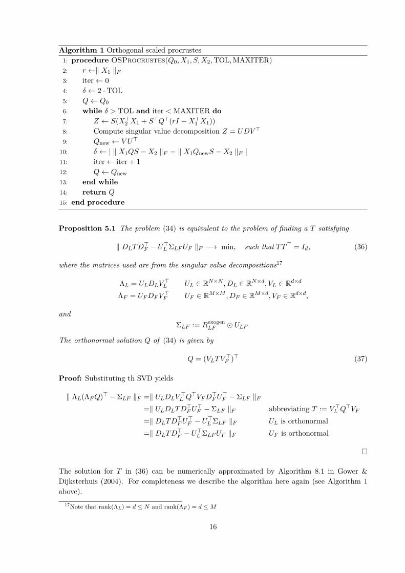
Algorithm 1 Orthogonal scaled procrustes1: procedure OSProcrustes(Q0, X1, S, X2, TOL, MAXITER)2: r ←∥ X1 ∥F3: iter← 04: δ ← 2 · TOL5: Q← Q06: while δ > TOL and iter < MAXITER do7: Z ← S(X⊤
2 X1 + S⊤Q⊤(rI −X⊤1 X1))
8: Compute singular value decomposition Z = UDV ⊤
9: Qnew ← V U⊤
10: δ ← | ∥ X1QS −X2 ∥F − ∥ X1QnewS −X2 ∥F |11: iter← iter + 112: Q← Qnew13: end while14: return Q
15: end procedure
Proposition 5.1 The problem (34) is equivalent to the problem of finding a T satisfying
∥ DLTD⊤F − U⊤
L ΣLF UF ∥F −→ min, such that TT ⊤ = Id, (36)
where the matrices used are from the singular value decompositions17
ΛL = ULDLV ⊤L UL ∈ RN×N , DL ∈ RN×d, VL ∈ Rd×d
ΛF = UF DF V ⊤F UF ∈ RM×M , DF ∈ RM×d, VF ∈ Rd×d,
andΣLF := Rexogen
LF ⊙ ULF .
The orthonormal solution Q of (34) is given by
Q = (VLTV ⊤F )⊤ (37)
Proof: Substituting th SVD yields
∥ ΛL(ΛF Q)⊤ − ΣLF ∥F =∥ ULDLV ⊤L Q⊤VF D⊤
F U⊤F − ΣLF ∥F
=∥ ULDLTD⊤F U⊤
F − ΣLF ∥F abbreviating T := V ⊤L Q⊤VF
=∥ DLTD⊤F U⊤
F − U⊤L ΣLF ∥F UL is orthonormal
=∥ DLTD⊤F − U⊤
L ΣLF UF ∥F UF is orthonormal
The solution for T in (36) can be numerically approximated by Algorithm 8.1 in Gower &Dijksterhuis (2004). For completeness we describe the algorithm here again (see Algorithm 1above).
17Note that rank(ΛL) = d ≤ N and rank(ΛF ) = d ≤ M
16
The objective is to find a Q that minimizes
∥ X1QS −X2 ∥F , subject to QQ⊤ = I,
where S has entries on its diagonal only.The stopping of the numerical procedure is controlled by the maximal number of iterations(MAXITER) and the tolerance in change of the Frobenius norm (TOL) in the objective above.As initial guess the trivial transformation Q0 = I can be used.
6 Applying the calibration to market data
6.1 Summary of the Calibration Procedure
The following scheme summarises the steps of the calibration procedure, bringing together thesteps discussed in the previous sections and assuming the calibration of the (domestic) interestrate LMM has already been carried out.18
I. Preliminary calculations applied to the LMM calibration outcome.
1. For each calendar time ti (1 ≤ i ≤ nL):
(a) Compute the covariance matrix ΣLi as in (20).
(b) Decompose ΣLi into λL
i using PCA as described in Section 3.
II. Hybrid Calibration.
1. Calibrate on all commodity data to obtain the global θF , and ηF .
2. Calibrate on all data to obtain the skew term-strucutre BF , see Remark 3.3.
3. For each calendar time ti (1 ≤ i ≤ nF ):
(a) Compute the covariance matrix ΣFi as in (20).
(b) Decompose ΣFi into UF
i using PCA as described in Section 3.(c) Compute the rotation matrix Q using Algorithm 1
4. Compute forward prices from futures prices using (26).
5. Compute model options prices on forwards.
6. Continue with Step 3 until a sufficiently close fit to commodity market instru-ments and assumed cross–correlations is reached.
The dynamics of the thus calibrated hybrid Commodity LMM with time-dependent SLV canthen be written as follows. Let W be a d-dimensional Brownian motion and denote by λL
i,j andλF
i,j the d-dimensional vectors in ΛL and ΛF of volatilities for calendar times t ∈ [ti−1, ti) and
18Note that we must iterate over repeated calibration to the commodity market and to the cross–correlations,as the conversion of commodity futures into forwards depends on cross–correlations.
17
Jan14 Apr14 Jul14 Oct14 Jan1540
50
60
70
80
90
100
110
120
Futu
res
Pric
es
1M1Y2Y4Y
Jan14 Apr14 Jul14 Oct14 Jan15
15
20
25
30
35
40
45
50
55
Impl
ied
Vol
atili
ty (%
)
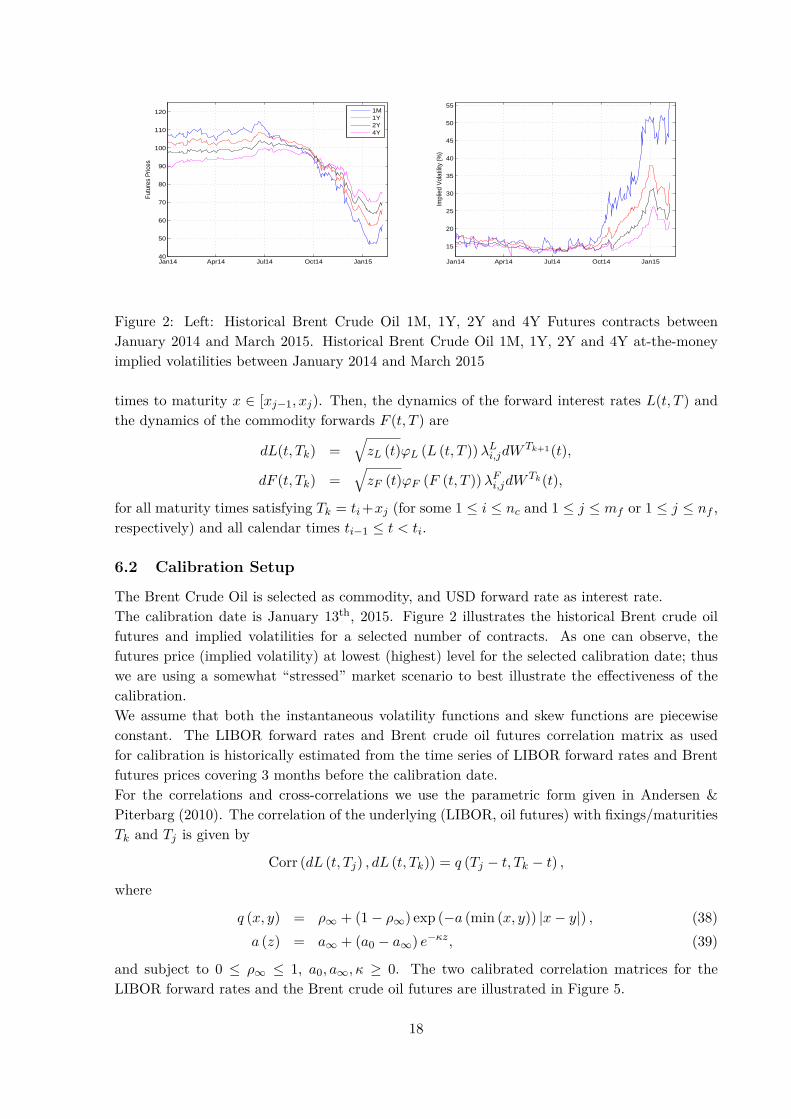
Figure 2: Left: Historical Brent Crude Oil 1M, 1Y, 2Y and 4Y Futures contracts betweenJanuary 2014 and March 2015. Historical Brent Crude Oil 1M, 1Y, 2Y and 4Y at-the-moneyimplied volatilities between January 2014 and March 2015
times to maturity x ∈ [xj−1, xj). Then, the dynamics of the forward interest rates L(t, T ) andthe dynamics of the commodity forwards F (t, T ) are
dL(t, Tk) =√
zL (t)φL (L (t, T )) λLi,jdW Tk+1(t),
dF (t, Tk) =√
zF (t)φF (F (t, T )) λFi,jdW Tk(t),
for all maturity times satisfying Tk = ti +xj (for some 1 ≤ i ≤ nc and 1 ≤ j ≤ mf or 1 ≤ j ≤ nf ,respectively) and all calendar times ti−1 ≤ t < ti.
6.2 Calibration Setup
The Brent Crude Oil is selected as commodity, and USD forward rate as interest rate.The calibration date is January 13th, 2015. Figure 2 illustrates the historical Brent crude oilfutures and implied volatilities for a selected number of contracts. As one can observe, thefutures price (implied volatility) at lowest (highest) level for the selected calibration date; thuswe are using a somewhat “stressed” market scenario to best illustrate the effectiveness of thecalibration.We assume that both the instantaneous volatility functions and skew functions are piecewiseconstant. The LIBOR forward rates and Brent crude oil futures correlation matrix as usedfor calibration is historically estimated from the time series of LIBOR forward rates and Brentfutures prices covering 3 months before the calibration date.For the correlations and cross-correlations we use the parametric form given in Andersen &Piterbarg (2010). The correlation of the underlying (LIBOR, oil futures) with fixings/maturitiesTk and Tj is given by
Corr (dL (t, Tj) , dL (t, Tk)) = q (Tj − t, Tk − t) ,
where
q (x, y) = ρ∞ + (1− ρ∞) exp (−a (min (x, y)) |x− y|) , (38)a (z) = a∞ + (a0 − a∞) e−κz, (39)
and subject to 0 ≤ ρ∞ ≤ 1, a0, a∞, κ ≥ 0. The two calibrated correlation matrices for theLIBOR forward rates and the Brent crude oil futures are illustrated in Figure 5.
18

0
2
4
6
0
1
2
3
0.4
0.5
0.6
0.7
0.8
0.9
Calendar TimeForward Time
0
2
4
6
0
1
2
3
0.2
0.4
0.6
0.8
1
1.2
Calendar TimeForward Time
Figure 3: Left: The calibrated implied volatility term structure for the swaption cube. Right:The calibrated implied skew term structure for the swaption cube.
0 1 2 3 4 50.35
0.4
0.45
0.5
0.55
0.6
0.65
0.7
Expiry
Effe
ctiv
e A
TM V
olat
ility
Mkt 1Y tenorMod 1Y tenorMkt 2Y tenorMod 2Y tenorMkt 3Y tenorMod 3Y tenor
0 1 2 3 4 50.4
0.5
0.6
0.7
0.8
0.9
1
1.1
1.2
1.3
1.4
Expiry
Effe
ctiv
e S
kew
Mkt 1Y tenorMod 1Y tenorMkt 2Y tenorMod 2Y tenorMkt 3Y tenorMod 3Y tenor
Figure 4: Left: The calibrated effective volatility λmktn,m for the swaption cube. Right: The
calibrated effective skew bmktn,m for the swaption cube
6.3 The Interest Rate Calibration
The calibration of the SLV–LMM for the USD interest rate market was conducted based onPiterbarg (2005) by first performing a pre–calibration to fit the SLV–LMM, with constant pa-rameters for each tenor and expiry, to the swaption cube. Figure 4 illustrates the obtainedeffective at–the–money volatility λmkt
n,m and effective skew bmktn,m for each tenor Tn and expiry Tm.
These obtained model parameters then serve as target values in the main calibration whencalibrating the volatility and skew term–structure as described in Piterbarg (2005). Figure 3shows the resulting volatility and skew term-structure obtained by the main calibration. Figure4 shows the quality of fit effective at–the–money volatility λmkt
n,m and effective skew bmktn,m. The
overall model fit to the implied volatility is very good. Moreover, we chose dL = 4 factors, whichtypically explains about 99.99% of the overall variance.
6.4 The Cross-Calibration
The calibration of the Brent Crude Oil futures was achieved by the method described in Section3. The market instruments are futures and options on futures. Figure 7 shows the calibratedvolatility and skew surface. Calendar and forward times go out to 3 years, and although on the
19

0
2
4
6
0
2
4
60.7
0.75
0.8
0.85
0.9
0.95
1
Forward TimeForward Time 0
2
4
6
0
2
4
60.8
0.85
0.9
0.95
1
Forward TimeForward Time
Figure 5: Left: The historically estimated LIBOR forward rate correlation matrix. Right: Thehistorically estimated Brent crude oil futures correlation matrix.
0
2
4
6
0
2
4
6−0.5
0
0.5
1
Commodity ForwardsInterest Rate Forwards 0
2
4
6
0
2
4
60
0.01
0.02
0.03
0.04
Commodity ForwardsInterest Rate Forwards
Figure 6: Left: The target cross-correlation matrix (green) estimated from historical futuresreturns, the rotated cross correlation (blue) and the un-rotated cross correlation (grey) matrix,for the calendar time 0. Right: The absolute differences between target and rotated cross-correlations.
exchange futures with expiries in every month are traded, we chose the calendar and forwardtime vectors to be unequally spaced (while still calibrating to all traded instruments), [0, 1M,3M, 6M, 9M, 1Y, 2Y, 3Y]. This setup speeds up the calibration without losing much structurein the volatility surface, since the market views futures with long maturity to have almost flatvolatility. For weighting in the calibration objective function we have chosen ηλ,1 = ηb,1 = 0.1(time homogeneity, i.e. smoothness in calendar time direction), ηλ,2 = ηb,2 = 0.01 (smoothnessin forward time direction).The exogenously given target cross-correlation matrix (calculated from the historical time seriescovering 3 months before the calibration time) and the estimated cross-correlation from historicalfutures returns and the cross-correlation matrix for the calendar time that fitted worst areillustrated in Figure 6.Finally, we link both separately calibrated volatility matrices to one set of stochastic factors.Table 1 shows how much of the overall variance, i.e. of the sum of variances over all factors,can be explained by the leading factors, when the factors are sorted according to decreasingcontribution to total variance of the commodity forwards. The first two factors already account
20

Number of Factors 1 2 3 4 5 . . . 19Percentage of 98.14 99.84 99.96 99.98 99.99 . . . 100Overall Variance
Table 1: The percentage of overall variance that can be generated by the first i factors, obtainedfrom PCA of the commodity forward covariance matrix for the first calendar time t1.
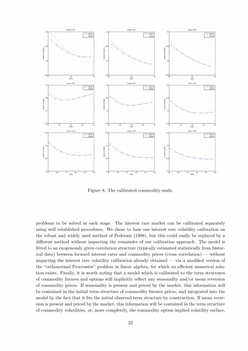
for more than 99% of the overall varianceNote that if it is necessary to interpolate the forward interest rate volatility matrix in order tomatch the calendar times of the commodity volatility matrix, the forward rate covariance matrixwill change and, hence, eigenvalue decompositions of the calendar time adjusted covariancematrices yield different results than an eigenvalue decompositions of the original covariancematrices as used for calibration. However, these differences should not be substantial as long asthe calibrated volatility matrix is sufficiently smooth in calendar time.The model fit to the commodity implied volatility is illustrated in Figure 8.
0
1
2
3
01
23
45
0.2
0.3
0.4
0.5
0.6
0.7
Calendar TimeForward Time
0
1
2
3
01
23
450
0.2
0.4
0.6
0.8
Calendar TimeForward Time
Figure 7: Left: The calibrated commodity volatility surface. Right: The calibrated commodityskew surface.
7 Conclusion
As the market data example in the previous section demonstrates, the LMM approach to termstructure modelling remains is one of the most flexible in allowing for good calibration of themodel to market data, even when it is extended to allow for market quotes across multiplestrikes (volatility “skews” and “smiles”) and the integration of (and correlation between) multiplesources of risk — commodity and interest rate risk in our present example. This is due to actualmarket observables (in particular forward LIBORs) being modelled directly and model pricesfor calibration instruments (e.g. caps/floors, swaptions, commodity futures and options) beingavailable either in exact or accurate approximate closed form.The dynamics of all market variables can be expressed in terms of the same, vector–valuedBrownian motion and correlation between market variables is obtained via the sum productsof the respective vector–valued volatilities. As a consequence, the calibration across multiplesources of risk can be broken down into stages, simplifying the high–dimensional optimisation
21
40 50 600.35
0.4
0.45
0.5Expiry: 0.16Y
Strike
Implie
d V
ola
tilit
y
ModelMarket
40 50 600.35
0.4
0.45
0.5Expiry: 0.24Y
Strike
Implie
d V
ola
tilit
y
ModelMarket
40 50 600.35
0.4
0.45
0.5Expiry: 0.32Y
Strike
Implie
d V
ola
tilit
y
ModelMarket
50 60 70 80 900.25
0.3
0.35
0.4Expiry: 0.58Y
Strike
Implie
d V
ola
tility
ModelMarket
50 60 70 80 900.25
0.3
0.35
0.4Expiry: 0.82Y
Strike
Implie
d V
ola
tility
ModelMarket
50 60 70 80 900.25
0.3
0.35
0.4Expiry: 1.28Y
Strike
Implie
d V
ola
tility
ModelMarket
50 60 70 80 90 1000.2
0.25
0.3
0.35Expiry: 1.79Y
Strike
Implie
d V
ola
tility
ModelMarket
50 60 70 80 90 1000.2
0.25
0.3
0.35Expiry: 2.28Y
Strike
Implie
d V
ola
tility
ModelMarket
50 60 70 80 90 1000.2
0.25
0.3
0.35Expiry: 2.79Y
Strike
Implie
d V
ola
tility
ModelMarket
Figure 8: The calibrated commodity smile.
problems to be solved at each stage. The interest rate market can be calibrated separatelyusing well established procedures. We chose to base our interest rate volatility calibration onthe robust and widely used method of Pedersen (1998), but this could easily be replaced by adifferent method without impacting the remainder of our calibration approach. The model isfitted to an exogenously given correlation structure (typically estimated statistically from histor-ical data) between forward interest rates and commodity prices (cross–correlation) — withoutimpacting the interest rate volatility calibration already obtained — via a modified version ofthe “orthonormal Procrustes” problem in linear algebra, for which an efficient numerical solu-tion exists. Finally, it is worth noting that a model which is calibrated to the term structuresof commodity futures and options will implicitly reflect any seasonality and/or mean reversionof commodity prices. If seasonality is present and priced by the market, this information willbe contained in the initial term structure of commodity futures prices, and integrated into themodel by the fact that it fits the initial observed term structure by construction. If mean rever-sion is present and priced by the market, this information will be contained in the term structureof commodity volatilities, or, more completely, the commodity option implied volatility surface,
22
to which the model is calibrated.19
19Specifically, mean reversion would manifest itself in the market as a downward sloping term structure ofcommodity option implied volatilities.
23

BIBLIOGRAPHY
Andersen, L. & Brotherton-Ratcliffe R. (2005), ‘Extended Libor Market Models with StochasticVolatility’, Journal of Computational Finance 9, 1–40.
Andersen, L.B & Piterbarg, V. (2010), Interest Rate Modeling: Models, Products, Risk Man-agement. In three volumes.
Black, F. & Scholes, M. (1973), ‘The Pricing of Options and Corporate Liabilities’, Journal ofPolitical Economy 81(3), 637–654.
Brace, A., Gatarek, D. & Musiela, M. (1997), ‘The Market Model of Interest Rate Dynamics’,Mathematical Finance 7, 127–154.
Choy, B., Dun, T. & Schlögl, E. (2004), ‘Correlating Market Models’, Risk, 17, 124–129.
Cortazar, G. & Schwartz, E. S. (1994), ‘The Valuation of Commodity Contingent Claims’,Journal of Derivatives 1, 27–39.
Cox, J.C., Ingersoll, J.E. & Ross, S.A. (1981), ‘The Relation between Forward Prices and FuturesPrices’, Journal of Financial Econometrics 9, 321–346.
Gibson, R. & Schwartz, E. S. (1990), ‘Stochastic Convenience Yield and the Pricing of OilContingent Claims’, Journal of Finance 45, 959–976.
Golub, G. & Van Loan, C. (1996), Matrix Computations (3rd ed.), Johns Hopkins.
Gower, J.C. & Dijksterhuis, G.B. (2004), Procrustes Problems, Oxford University Press.
Grzelak, L. & Oosterlee, C. (2011), ‘On Cross-Currency Models with Stochastic Volatility andCorrelated Interest Rates’, Applied Mathematical Finance, 1–35.
Hagan, P., Kumar, D., Lesniewski, A. & D. Woodward. (2002), ‘Managing Smile Risk’, WilmottMagazine September, 84–108.
Heath, D., Jarrow, R. & A. Morton. (1992), ‘Pricing and the Term Structure of Interest Rates:A New Methodology for Contingent Claims Valuation’, Econometrica 60, 77–105.
Jamshidian, F. (1997), ‘LIBOR and Swap Market Models and Measures’, Finance & Stochastics1, 293–330.
Koschat, M.A. &D.F. Swayne (1991), ‘A weighted Procrustes criterion’, Psychometrika 56,229-223.
Miltersen, K. (2003), ‘Commodity Price Modelling that Matches Current Observables: A NewApproach’, Quantitative Finance 3, 51–58.
Miltersen, K., Sandmann, K. & Sondermann, D. (1997), ‘Closed Form Solutions for Term Struc-ture Derivatives with Log-Normal Interest Rates’, Journal of Finance 52, 409–430.
Miltersen, K. & Schwartz, E. (1998), ‘Pricing of Options on Commodity Futures with StochasticTerm Structures of Convenience Yield and Interest Rates’, Journal of Financial and Quanti-tative Analysis 33, 33–59.
Musiela, M. & Rutkowski, M. (1997), Martingale Methods in Financial Modelling, SpringerVerlag.
Pedersen, M.B. (1998), ‘Calibrating Libor Market Models’, SimCorp Financial Research Work-
24

ing Paper.
Rebonato, R., McKay, K. & R. White (2009), The SABR/LIBOR Market Model, Wiley.
Pilz, K.F. & Schlögl, E. (2013), ‘A hybrid commodity and interest rate market model’, Quanti-tative Finance, 13, 543–560.
Piterbarg, V. (2005b), ‘Time to smile’, Risk Magazine, 18, 71–75.
Schlögl, E. (2002), ‘Arbitrage-Free Interpolation in Models of Market Observable Interest Rates’,In K. Sandmann & P. Schonbucher (Eds.), Advances in Finance and Stochastics, Springer,Heidelberg.
Schlögl, E. (2002), ‘A Multicurrency Extension of the Lognormal Interest Rate Market Models‘ Finance & Stochastics 6, 173–196.
Schwartz, E. S. (1982), ‘The Pricing of Commodity–Linked Bonds’, Journal of Finance 37, 525–539.
Schwartz, E. S. (1997), ‘The Stochastic Behavior of Commodity Prices: Implications for Valua-tion and Hedging’, Journal of Finance 52, 923–973.
25