c national advisory committee c for … · c < national advisory committee ... woods,...
TRANSCRIPT

(s) I\
cc<
NATIONAL ADVISORY COMMITTEE
FOR AERONAUTICS ‘L
TECHNICAL NOTE 2643
SPAN LOAD DISTRIIXTTIONS RESULTING FROM ANGLE OF ATTACK,
ROLLING, AND PITCHING FOR TAPERED SWEPTBACK WINGS
WITH STREAMWISE TIPS
SUPERSONIC LEADING AND TRAILING EDGES
By John C. Martin and Isabella Jeffreys
Langley Aeronautical LaboratoryLangley Field, Va.
I
Washington
July 1952
. ..,.A; “; ‘v
,- -irri.-d
/.
>
,. -
— --.——-—- ..–-. . . . . . -.. .. ..— — .
https://ntrs.nasa.gov/search.jsp?R=19930083555 2018-08-20T07:51:04+00:00Z

TECHLIBRARY KAFB. NM
,L
—
lIllnllllllilllimllol011b5b43
NATIONAL ADVISORY COMMDTEE F(IRAERONAI%l?ICS
TECHNICAL NOTE 2643
SPAN LOAD DISTRIBUTIONS RESUIX’INGFROM ANGLE OF ATTACK,
ROLLDIG, AND PITCHING F(IRTAPERED SWEW33ACK WINGS
W131HEWREAWISE T12S
SUPERSONIC LEADING AND TRAIIJNG EWES
By John C. Msrtin and Isabella Jeffreys
SUMMARY
On the basis of the linearized sup&sonic-flow theory the span load&Lstributions resulting from constant angle of attack, from steady rolling,and from steady pitching were calculated for a series of thin sweptbacktapered w@gs with stresmwi.setips ad. with supersonic lea-g and _&ailingedges. The results are valid for the Mach nmib~ range for which theMach line from eith~ wing tip does not intersect the remote half-tig.
The results of the analysis are presented as a series of designChsxts. Some illustrative variations of the spanwise distribtiion ofcircuktion with the variouE
.design parameters sre also presented.
INTRODUCTION
.
A lmowledge of aerodynamic spanwise loatig is of great value inperforming aerodynamic calculations. In references 1 to 4 the Unearizedupwash behind a lifting wing is shown to be largely determined by thespamise loading except for the region close to the trailing edge. Itmay also be demonstrated that, except in the vicinity of the trailingedge, the sidewash velocity component is also largely determined by thespanwise loadhg. The ah of the present pap= is to determine spanwiseloadings for a series of thin sweptback tapered wings with stresmwisetips and with supersonic leadhg and hailing edges. These spanwiseloadings can be utilized in connection with the estimation of flow fieldsalthough the results of the analysis my also be applied to problems inaerodynamic loads and aeroelasticity. .
The spanwise distribution of circulation resulting from a constantangle of attack was eval-ted chieflj because of the significance of the
.-. ..__— . . .. .. -..—- ,.. ,..—__ ___ ..— —---- . ..—

2 ..,,,, NACA TN 2643
downwash induced by the wing on the horizontal tail surfaces. similarly, ,“Ithe spanwise distribution of cticulation resulting from a constant rateof roll was evaluated principally because of the significance of thevelocities induced by the wing on the tail-surface contribution tostability and damping. The spanwise distribution of circulation resultingfrom a constant rate of pitch was evaluated because of the possiblehportance of the downwash tiduced by the pitching wing on the horizontaltail surfacds and because the downwash resulting from a pitching wing isone component of the downwash induced by a wing with a constant verticalacceleration. (See reference 5.)
This paper presents calculated curves for the spanwise distributionof circulation (the spanwise distribution of circulation is proportionalto the spanwise loaclbg) resulthg from a constant angle of attack, aconstant rate of roll.,and a constamt rate of pitch. The wings consideredhave an srbitraty tap= ratio, leading and trailing edges that arestraight across the semispan and swept at a constant angle, and tipsthat are parallel to the free-stream direction. The results are validfor the range of Mach number for which the leading and trailing edgesare supersonic.
The results of the analysis are given in the form of generalizedequations for the spanwise distribution of circulation resulting froma constant angle of attack, a constmt rate of roll, and a constant rateof -pitch. A series of design curves is presented from which rapidesthation of the spanwise distributions of circulation can be madefor given values of aspect ratio, taper ratio, Mach nuniber,and leading-edge sweep. Some illustrative variations of the spsnwise distributionsof circulation are also presented.
SYMBOLS
A“ aspect ratio
B=d=”h &panwise coordinate of intersection of trailtig edge of wing
and Mach line from *g tip
cl section lift ‘coefficient
% pressure-clifference coefficient
c chord (mibscript r refers to root chord)
E mean aerodynamic chord
,1
.
.
_——.— ._— — .

NACA TN 26k3
d
e
13(xl)
Q(X,Y), @(x,Y)
H
b
.
3
spanwise coordinate of intersection of trai3Jng edgeof wing and Mach line reflected from wing tip
spanwise coordinate of titersection of trailing edgeof wing and Mach line from leading edge of wing
expression for that part of boundary of area S1
not made q of Mach lties from point (x,y)(seefig. 3)
limits of integration (see fig. 3)
distance in chord lengths from wing apex to center-.of-gavity location for wing with a static marginof 0.05E
wing span
cot Amk=—=All(l+ x)
cot A AB(l+ A) - 41ilB(l- k)
CC2 spanwise loaQ
M
m
P
J?
v
x, y, z
Mach number ‘
co-tA
defined by equation (6)
rate of roll
rate of pitch “
area of integration .-
free-stream veloc”ity,. ,,
rectangular coordinates (x-aXi’s“parallelto free-stream &Lrection)
auxiliary rectangular coordinates
angle of attack
spanwise distribution of circulationequation (2))
(defined by
\
.— .- —.-—. — .— —

—.. ..— — .
4 NLICATN 2643.
9 velocity Totential on wing wer surface
A sweep of wing leading edge (see fig. 1)
Am sweep of wing trailing edge (see fig. 1)
L taper ratio
$indicates a closed line integral
subscript:
TE refers to wing trai13ng edge
ANAIXSIS
Scope .
The analysis is limited to calculations of the spanwise distributionsof circulation for wings of vanishingly small thiclmess that have zero
.
c?3atEr. The results me valid for a range of supersonic speeds for.
which the leading and trailtig edges are supersonic (the components offree-stream velocity normal to the edges are supersonic). The wingconfigurations considered are defined by the information and sketchesgiven in figure 1. These wings have an sxbitrary taper ratio, stream-wise tips, and sweptback lead3ng edges, although the trailing edges maybe either sweptback or sweptforward. A further restriction is that theMach line from either tip may not titersect the remote half-tig.
Method
Basic considerations.- The evaluation of the spanwise loadings
generally requires ,thelmowledge of the pressure distribution on thewing surface or the knowledge of the perturbation velocity potentialalong the wing trailing edge. These-two quantities are related by thefollowing expression:
(1)
$. . . . .—_— — ——-—— ———— -——— —. ——–. -—— . —.——— -— -— — —

MCA m 2643 5
The spanwise distribution of circulation is related to the spanwiseloading and the trailing-edge potential by the following equation:
(2)
In the remainhg sections the spanwise distribution of circulation willbe used h preference to the spanwise loading since flow-field calculationsare generally set up in terms of the spanwise distribution of circulation.
Determination of the trail~-edge potential.- The potential
function @ must satisfy the linearized partial-differential equationof steady flow and the boundary conditions that sre associated with thewtig in its prescribed motion. The boundary conditions on a w5ng performingthe motions considered here are:
For a constant angle of attack, /
92 = -av. For a constant rate of roll,
f$z= -w
(z = o) (3)
(z = o) (3)
For a constant rate of pitch,
$2 = .~ (z = o) (3C)
Note that, within the fruework of the linearized theory, the boundarycondition for a ~ with a constant rate of roll is also the boundarycondition for a w@ which has a l@ear lateral twist and that theboundary condition on a wing with a constant rate of pitch is also theboundary condition on a wing which has linear camber.
The potential along the wing trailing edge can be deterndnedbyEward~s method (reference 6). From this reference the potential atany petit on the upper surface of the wing may be expressed as
i
J-TJ
$Z@(x)y) =-~ ~1 q (k)
n ‘1 (x - X1)2 -B2(Y - D)2
.— .—— . ..__— —.. . .. —___ —.–--— ——— —— ———. —-—--— J,,

—
6 NM!flTN 2643
The area of integration S1 is the area of the wing ph form tithti
the “effective” forwardMach cone Yrom the petit (x,Y)”. Fi~e 2 showssuch a region of integration. For the motions of the wing consideredherein, the potential on the wer surface of the wing maybe obtainedby substituting equations (3) tito equation (4) and performing theindicated titegations.
The evaluation of the inte~als involved in finitlmgthe potentialcan, however, be shplified by ~ we of we we~-wo~ re~tion(reference i’,p. 181)
J @(q,Yl).,. dlq d-y,= - &’(x,,Y,) W, ~
Rrom a comparison of
seen to be given by
(5)~Yl d
—
equations (4) and (5) the function P(xl,Y1) is
(,’,’$Z
P(xl,yl) = - * dy~
(X - X1)2 - B2(y - ~)2
(6)
Hencej from equations (3), (k), (5), and (6) the potential on the wp=surface of a wing is as follows:
For a constant angle of attack,
For a constant rate of roll,
(7) ‘
1-lB(Y -XL) ~1
(X- X1)2 -B2(y-Y~)2+Y Sin ~-x
1
.. (8)
n,
.—
..
.

NACA TN 2643 7
For
Thethefor
For
a constant rate of pitch,
$&y) .S$
-lB(Y - ~) ~1
Ja3s1~sti .-.1(9)
line integrals in equations (7) to (9) along the Mach lines from.
petit (x,Y) can be easily evaluated. The folluwing expressionstie potentials are obtained:
a constant angle of attack,
[9(X,Y) = ~ 2x - gl(x,y) -
2B.2,X,YI] +:’-’-’:) sKIB~x--g:~ dq
.
For a constant rate of roll,
9(X,Y) = g [~ - g-J(x,Y)- 132(x,Y)l+L J
Pq2(4
z J {J(x - x& -
Q(x) ~ ‘2[Y - ‘(X1!2+
For a constant
-1y sin
x - xl 1rate of pitch,
ax,
(lo)
(1.2)
(II)
●
. . . . . .——_. ___ .. . .. –—— --y .— ———— ———.— -. -.— .—— _ ___ _

8 NACAm 26k3
where g(xl) is the expression for that psrt of the boundary of the
area S1 that does not contain the Mach lines from the point (x,y),
and where gl(x) and g2(x) are the limits of integration which are
actually the end potits of the g(xl) boundsry. (See fig. 3.) Note
that eqwtions (10), (U), and (1.2)are applicable to any plan form towhich E&vard?s method can be applied. Since there are no singularitiesin the titegrands of these eqyations they can be evaluated numericallywithout Ufficulty.
ItlHJLTs
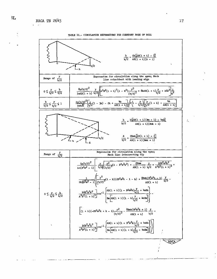
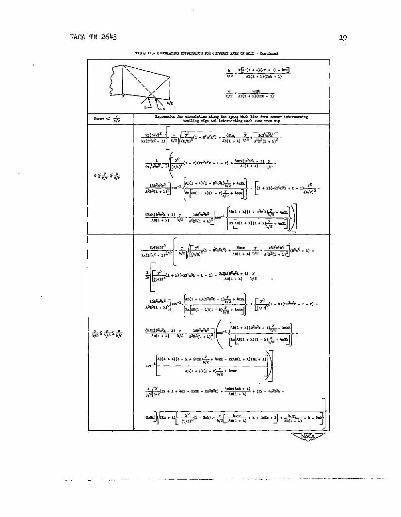
Expressions for the trailing-edgepotentials were either takenfrom table I of reference 8 or found by the use of equations (10), (U),and (12). The spsmdse distribution.of circulation was expressed as afunction of y by.stistitutingthe equation for the trailing edge intothe expressions for the potential &fference between the upper and lowersurfaces of the wing. These expressions for the spanwise distributionsof circulation are presented for constant angle of attack in table 1,for constant rate of roll in table II, and for constant rate of pitchh table III. The formulas sre valid for either sweptforwaxd or swept-back trailtig edges, the proper applications depending on the sign of k.
“
“
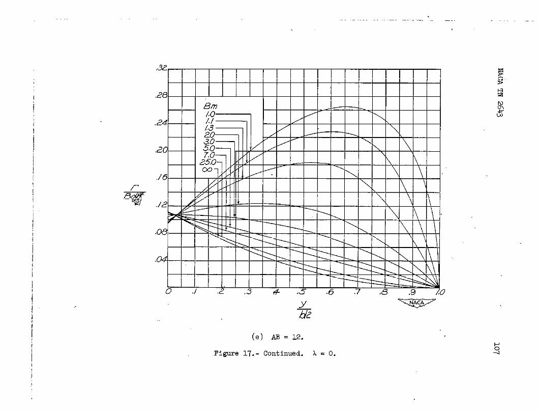
The results of the calculations for the spahwise &Lstribution ofcirculation for w3ngs with a constant angle of attack are presented infigures 4 to 9. An index of these figures is given h table IV. Similarresults for constant rate of roll are plotted in figures 10 to 15 andfor constant rate of pitching about the ~ apex in fi~es 16 to 21,with hlexes of figures for the two types of mothne listed in tables Vand VI. These figures sre equally applicable for sweptback or sweptforwardtrailing edges.
The results of the calculationspresented in figures 16 to 21 arefor wings pitchtig about theti apex. The spsmtise distribution ofcticulation for a w3ng pitchtig about an srbitrary point located adistance xd downstream of the wing apex is given by
(13)
where the subscript q tidicates the spanwise distribution of circulationassociated with a pitcldng wing and the mibscript a tidicates thespanwise distribution of circuJ.ationassociated with a wing at a constantangle of attack.
-.
..— — -——— —— .— —..

2L9NACA TN 2643
Note that,several lifttig
M the total cticulation of a wing is divided smongkhes, the distribution of circulation associated with
each lifting l~e cm-be determined by the superposition of the &lstri-butions of circulation associated with a number of wings. For thisreason the calculations were extended to rather large values of theparameter AB.
Figures 4 to 21 indicate that in many cases the spanwise distributionof circulation can be approximated very closely by WWple curves. Thusit is to be expected that for these cases the flow field behind thewings coul.dbe calculated approximately.by making use of these simplecurves that approxhate the actual spanwise distribution of circulation.
Illustrative curves of the spanwise distribution of circulation forwings with a constant angle of attack, a constant rate of roll, andaconstant rateof pitch are presented in figures 22, 23, and 24,respectively. ~ figure 24 the values presented were calculatedlyequation (13) for center of gravity located to provide a static margin ‘-of 0.0~5. These figures show the effect on the spanwise distributionof circulation of varying each of the parameters - aspect ratio, taperratio, Mach number, and leading-edge sweep - separately. Some specificvariations of the spanwise distribution of circulation with the positionof the axis of pitch me presented in figure 25.
CONCLUDING REMARK
On the basis of the steady linearized supersonic-flow theory thespanwise distribution of circulation resulting from constant angle ofattack, from steady rolling, and from steady pitching was determinedfor a series of thin sweptback tapered wings with streamwise tips andwith supersonic leading and trailing edges.
\
Langley Aeronautical LaboratoryNational Advisory Committee for Aeronautics
Langley Field, Vs., October 24, 1951
-.,.. .——. — —.—. -- ,-. --- ..—.— —— ——- — —- -

’10
REFERENCES, “. “
~ACA TN 2643
,, ....
1. Robtison, A.; and Hunte&Tod, J. Ho : _Bound and Tratig Vortices inthe Linearized Theory of Supersonic Flow, and the Downwash in tieWake of a Delta Wing. Rep. No. 10, College of Aero., Cranfield,(British), Oct. 1947.
.,2. Mirels; Harold, and Haefeli, ,RudolphC.: Line-Vortex Theory for
Calculation of Supersonic Downwash. ,NACA Rep. 983, 1950:,.
3. Martin, John C.: The Calculation of Downwash Be&d Wings of ArbitraryPlan Form at SupersonicSpeeds. -NACATN 213S, 1950.
,,,“4. Haefeli,”Rudolph C...Mirelsj H~old, and Cmmnlngs; ~OhIlL.:. charts
.for Estimating Downwaih Behind Rectangular, Trapezoidal, audTriangular Wings at SWqsonic Speeds. NACA TN 2141, 1950.
,-5. Ribner, Herb&t” S.: “““Ttie-Depend@ -Downwashat the Tail and the
Pitchbg Moment Due to Normal Accel~ation at Supersonic Speeds.NACA ‘TN,2042,195U. ,,~.. .:. , .~” -
6. Ev-vard,John C.: Use o? Sotice Distributions for EvalualxbgTheoretical Aerodynamics of Thin Finite Wings at Supersonic Speeds.NACA Rep. 951, 1950. , ,,: ~
7. Woods, Ike&rick S.: Advanced Calculus. Ginn and Co., 1934.
8. Harmon,”Sidney M., and Jeffreys, Isabella: !l?heoret~calLift andDsmping in Roll.of Thin Wings with Arbitrary Sweep and Taper ats~ersofic, Speeds. Sqmrsonic LeatLingand Trailing Edges. NACA -m 2114, 197).
.,, ,
.
. . . .
——. --——— ——. —.—. — .

NACA TN 2@3
TAUE I.- cEmmmaf=Fm=ImBmc m=x+!r Amlsc4AmAcI
11
8
-.——— . —_— ..z —.———-- ..—.- —— .——.——

12 NACA TN 2643
\
_.— — .-
.
.

13
.
-—. — —..._ —.— —-.—z ~ ——. .—.. .—— .—

I14 TWX m 2643
.
.
. .—-— ~ ——-— ——— —.

%$51b/2
TAB~ I.- CIWUIATIOE 2XFEESSICEIS FOR CfJH&T.ARTAH131E OF ATTACK - Continued
15
>
b\‘\ \ \ \ /
‘></
0 \ b/2h e
h AB(l + L)(BM+ 1) - @~“ EaB(l + x)
A. 4b/2 M(1 + ~)
__.—_ . . .. . __ _ .—— —

16 NACATN 2643
T#Br2 L- ~07(-S91W9kW(IX3m AI?O18WATlWK-Concluded
h AB(l+A)-4m“ AB(l+k)-ql -1)
.
—.—. —. ..— -—
NACA TN 2643 17
TABLE II.- cImmA!rIoN ExPmMIcEm FmcomTAm!RmEo F EuLL
.
—-—-. . .
h @B(l + x) - q~= AB(l +A)(k +1)
\0
\
//
R8nge of :~reeelcm for circulaticm along the spn; Mach
b/2 line coincident with leading edge
h @(b/2)2o~$z~v 1
#)--?&+8kAB(l+L)*+16k2-$3TCAB(1+ A)V
~s L$l W&y&(l - *)b/2 b/2 -=+m:+,~~pfi)~(l+k) +n:+,J
h k~(l + A)(Bu + 1) - 4mlJ—.b/2 AB(l + A)(mk + 1)
\d
/2w[@(l + L) - ZJ
/ IZ” AB(l+L)(EW+l)
Bxpreasim for circulatlca along the spn;Rmge of b=2 Msch line intersecting tip
[ ‘9’
2p(b/2)2 - y 1- B%%2) + h 2+16B%-W ~
kfl(B%# - 1) b/2~(b/2) AI!(1 + A) b/2 A%2(1 + A)*
- ([
~~& , -&.@ - k)(=%k- 1 -k) +h~~k; l~&-
16E?MW
] {[ ‘1-1AB(l+A)(1-B&k)b++hmko~L~A
b/2 b/2~cos BmAB(l +L)(l - k)%+ hJuIQ] -
[(1 + k)(-2B?m% + k - 1)* - -(B%% + 1) Y—-
(b/2)2 AB(l + x) b/2
.
i{}1 ,
AB(l + L)(1 + B%%= + 4mBk16B%-2 -1COB b/2
A2B2(1 + L)[ 1IWAB(l+A)(l+k)~+ b=
b/2 1
-.“ ‘-+w’-’
__. . .... __. —.. —- .— .—. .— — ———.

NACA TN 2643
mPJxn.- cE=ImrwKrF2m2IoE2 Pm caHwm2brE oFRoLL-cmtinnd
-Of$ Expremlcm for ci.rmlatim almg * p;Mach line Inta-aectingtip
2p(b/2)2
[+
1
‘ +2(w%a#)+~z+ ~ (B2m2.1)-
kx(Bw - 1)3/2bj (b/2) AB(l + A) b/2 A2E12(I+ X)2
[[
1 ~l+k)(-23%%+k-1)-h~~Aj l)fi-= (b/2)2
M2%%?
] [[
cm-l
7m(l+A)(B%%+lb’2 + k
+_&l-k)(#k -l-k)+A%’(l + X) (b/2)2
][2a AB(l+l)(l+ k@+-.b/2
1({ }X3(l+k)(l+wk- 1)*- 4&k
h<y<d 6mk(B?A - 1) Y I.Q%?#
@“m”m--1
A2(l + a) ~ - A%?(1 + X)2 E@l+A)(L- k~+kmi] -
r 11-
-1 (l+k)(l +k+=)b~+bmW?kAB (l+ A)(=+l)C*
AF@+L)(l-k~+4rEk
b
1 = 3k+l+knB-m-2#B%+&Ek(&l + 1)
+(Zk-4##k-% 12 A2(l - A)
aE2) (Em + 1)
Y{ 1}--&#l+Eak) +~~a+k+ 2mIQ+~+~-k-~
~(b/2)2
([
~l+k)(=%%+l-k)+m~~k; l)-&+sk?(F%2 - 1)~2 (V+)
H
162%%2 --1 1AB(l+x)(ak +l.. k~.. z@l+ L)(m-l)+4n2k+
A%?(l + A) AB(l+ L)(I+k~+ ~
d<~~l~ “ b/2
Ty*-m+l-m--+=w +(-a +41?#k -2&k)-
lf {4m2k(JlmB-1) 9
[Ba-1)----4+mk)+L - ~- 1 })
hm +k-=AB(l+x) k+2dTc+l+—
(b/2)2 b/2 A2(l + A) AI!(1+ x)
-.
.
.
——. — ——
NACATN 2643
mJL-ammIAmm 2xmm21msm ca2iYm E4nw FnIL—21ntlmd
19
+4-\ /-\ /
0 ‘>”/ \ b/2h e
e &uz“ A2(l+ Aj(w - 1)
Expmdcmf orcircnlatialalalg theSpsn;hcilllmhcmtal—btandng~dsa~ intwmd@ Mchlilmfrcm tip
9k-l~-
{b/2)
\
~ {[
lm%w --1 1A2(l+k)(l..#k)&+4m
Awl + A)2- (l+k)(-22%%
][YaA2(l+A)(l - k)++ ~
~ {[
6mk(* + 1) y I.!&# ~q
1
‘(l+ A)(l+**+*M(1 + A) ~-&#(~+x)
1BmAB(l+l)(l+kL+Xb/2
@(b/2)2
IIL
-$ *1-*+==+ 11-22(2%%)-X8(2%2 - 1)~2 D(l + X) b/2 Awl + A)
1L& =@l+k)(-2&#k +k-l)-w~~L; l~-&- .
] {[
162%w --~
}[
A20+w#k+l&+bm+=@l-k)(2E%%-l-k)+
A2B2(1+ A)2mAB(I + L)(I+ k%+ x]
(d {[
&k(E%l - 1)r 162%%? ~a
}
AB(l+A)(*-l)&-&kB
AM +x) ~ - &~l + ~)Rd2(.+wk%+ti] -
[—l-
A2(l+L)(l +k*alR)-&+wm-aA2(l +l)(M+l)
am-’
AB(l+L)(l-k~+Mk
r-L(m+l+ --am-awk)+-(p+; l)+(2k-4222k-* bj2
-c l-j~l+Bzk).+ y -~+k+~+l +-&&k -2zk(b/2)2 b/2 A2(l+ A) J
-.. — —— ——..— .—— — ———— —- -—— -———— -———— -—

~re.seim fm circulatim almg the p; Mach lina IYccneentw i.nt~ct.lng-%% ~ ~ ~ ~tietiingfichMm riwntip
p(b/2)2
[+ *(1 - k)(2B%#k -1- k) + ‘~:x~ 1) ; -
k%(B%2- 1)3/2 (b/2)
16B%aF
u
AB(l+X)(l +k+M!k)&+4m --(l+ L)(W+l)--1
A%(1 + X)2 AB(l + 1)(1 - k)-& +4mPL 1-+%=
[Myyb*m+l+ --2d%-2aRk)+ ~[:=y+2A&B%-
11 [[
2M% (m+l&2&(l+=)+_&-m~ ~,1
4mF&+k+~+ +
g~- k-m
Q?
\ 4mEk
\ $5” AB(l + k)(w - 1)\
\ //\
\o /’
h k~m(l + L)(M + 1) - 4~1\/ b/2
“e /h~“ AB(l + A)(i%k + 1)
Y Expmmlicmfar airculatica along the qmrl; math line-of~ from center intersecting trailing edge
[~
2p(b/2)2 y #1-B-)+ 8My 16B%42
kx(B%2 - 1) -ma—+ +
M(1 + N b12 *2B2(1 + ~)2
1
(!1- k)(2K%%- 1- k)+ ‘~~k; 1) _&-
=~~ (b/2)2
0%%
{ }
AB(l+X)(l - B%%) y + hmEkA-}W-l ~E,, , ~,(1 - k~+ -I - [al+ k)(-* + k -1, -
b/2
~ {E
*(B* + 1) Y 16B%%# --l
711
AB(l+L)(l+Bwk)by2+hl!kAB(l+a)=-A*(1 + L) h (1 + L)(l + k)b~ + km]
e<y<h P(b/2)2~“~nb~
[ 1+(1 -k)(Z3%% -1- k) + ‘;~A; 1) * - A%:~2
k2(lf# - 1)3/2 (b/2)
.
.— —
‘+&$=-
—.———
,
.
.
.
.

.
.,
NAC.ATN 2643 21
.
TABLE II. - CDEXJMTICWEDlE291~S FOBCCBW?AMTB&T2OFROIL- Ccattiei
F@4m0f~ ExpreeBicmfor drail.atlonalong the span; MachMmb/2 frm center Intersecting trailing edge
p(b/2)2
3([
9 (1-1@%%s-1-k)+8nlPk(B%k - 1) y—-
&(B% - 1) p= AB(l + A) b/2
+AB(l+X)(l +k+2@-&+Mk -2%AB(l+X)(Em+l)
~[
161iwk2 cm-lA%32(1+ A) AB(l + X)(l - k)~ + hdk
b/2
L$LS1b/2 bj2
[~-&k+ l+ MMBk-2&k)+ 4==&:;)l)+M#B’2k-
1( {- (Ea+l)‘2 Y
[ 1 })-~+k+~k+l +&-k-Bmk
-~l+~)+w AB(l+l)
--+-- ‘;2’’’:’”
0 -i-”b/2
Y Expnaelm for circulation almg the span; M9chline‘e ‘f * coincident with lea&Lngedge; unswepttrailing. .4@
hC%+$q ~:&/-~]
\
h<y<l
r
2p(b/2)2 ~ ~ - p +~=~” 3% b/2 .(:+LJ/~
.
--- .—— .-— -— --——— .. —-— .—— ..--—. — — — .—. .—— ————-—-—

22 NACA ~ 2643
,,.!
.
.
.
.
.——

NACA TN 2643 23
-
. . .—. —.—.. — — .—-— ..- ——— ——— ------- —-- —–---- --

24 NACA TN 2643
.
.
.
.
.
...—.—.-— —— ——- ———. .—--— --- —

L NACA TN 2643 25
TABIx HI. - CIWOIAT ICUlEXFI?XWGWFOBCOKO?AI?T_ OFPTl?C8
.
. . . . ..—. ——.— —.—- ——- —.—- .—— . ----- .-. _..—— .— ——— —--

26
Z14BIEm.- clmmATIm~?02 wrxcAm2AT2 aPPnc2-cmt-
NACA TN 2643
,
.
—---- . ..—-.— .—— ——. .

NACA TN 2643 27
.—. — .—— —.. — ——— . . .—

28 NACA ~ 2643
TABmm. —cmEmIAmolf mK-cEsmcm FmmmmiT RHewm-continwd
J
#
—.. —.— .—.——— — ——— ——-—— ..— ——.

NACA TN 2643
!rABm m.- cmmfATIaI ~cm FOR cofmAmRM3c3PlIcE -G3ntinm3d
$-w
29
.—— — .— —— —--- - . . —— ——— —

30 * NACA TN 2643
w Iu.- ~ul ~m m a2a2mm Mz2m PITc2-cmNamlQd
0
.
—. .

.
TABm .nI. - cImmATIIRl Bxm2E31cuwm cxumMm2A12 cQPmcE—conunma
31
.— ..— .—. ——- . - -- .-- —- —,—.

--- __..— _. . . . . . .-— ----- —— .. ——.

5L NACA TN 2643 33
TABIalv.-m5?3cLmv’Bm cImmATIaf AmiomE2PAHm cmrAE’rAmIEoFAmAcK,&
d2 I Em F@tn A2 I M I Figur A2 Bm F&meA2 I Ba Flgura
l..—
1.01.s2.0
;::
G1.11.32.0
A . 0.%(concluded)
—.
x . 1.03d)
6(c)(p. 47;
(s%
6(e)b. 49)
(%
COncl
i:;1.32.0
;::7-o
25.0.T
1.32.0
;::
L:.
1.01.11.32.03.0
2::.
1.01.11.32.0
;::
2::m.
A.o
(P.4*)
(329)
2 1.01.11.32.0S.o7.0.
6
8
12
12 I 1.0 7(0)
(P. 5s
T(P.56
+
1.11.32.0
R
&::.m 1.0
1.11.32.0
;::
&
3
3 9(b)(p. 64)
4
6
1.01.11.32.0
;::
;::.
—1.01.11.32.0
;::
;::.—1.01.11.3
;::7.05.0.
(No)
i
5(Ct(p. 1)
—4 1.0
1.11.32.0
;::
;::.
9(C)(P-@
9(d)(P-W
g(a)[p. 67)
3 8(a)(P.57)
8(b)(P.m)
8(c)
(P. 59)
20 6 1.01.11.3
x5.0
;::m
G1.11.32.03.05.07.05.0.
k 1.01.11.32.0
;::25.0
.
8 9(d)[p. 42)
8
(w)
7(b)(P.52)
7(c)(P. 53)
‘(:!dk)
t.
3
T
1.01.11.32.0
;::7.0
25.0mY
1.11.32.0S.o
2::.
6 1.01.11.32.0
;::
;::.
12
20
J
1.01.11.32.0>.07.05.0.
S(e)p. 43:
E 1.01.11.3?.03.05.01.0>.0.
9(f)p. @)
9(2)P. @)
7
8 8(d)(p.60)
8(e)[p.61)
1.0L.1L.3?.0].0r.o).0m—
5(f)p. 44)
1.01.11.3
“;:5.0
2::
Y1.11.32.0
;::
;::m
?0 LOL.1L-3!.01.0i.or.o;.0,
=*
12 1.01.11.32.0
;::7.05.0.
3 1.01.11.32.0
N7.0
6(a)(p. 45)
—4 1.0
1.11.32.0
;::
G
20 1.01.11.32.03.0>.07.05.0.
8(f):p. 62)
------ ... __ —z —— -- .

34 TN
v.- OJFQIL,
2643
A2 I h I Figure A2 m I Figure A2 I Ea I F* ABI B I FigureA-o . L = O.Zi ?.. 0.% A = 0.7s
(COmMsd) (mncluied) (mncluded)
: ::; (P?’m) 6 1-0 12(c) 22 14(f(P-79) u ;;
1.08 2.0 1.1 (:(:!) 1.1 t(P.9 )12 1.3 1.320 ;:: 2.0 1.3 2.0
2.0
3 1.0 U(a) ;:: 3.0 ;::1.1 (P--m1.3 2::
S.o2::
2.0 . .&
8 1.0 x?(d) . A . l.m1-3 (p.80) ~ lo2.0 13(f) 2
41.0
1.0 U(b) 1.1 (p.m) 1.1 (:(2)1.1 (P.72) ;:: 1.3 1.31-3 2.0 2.02.0 2:: 3.0
. 5.0 R;:: \ .
12 1.0 12(e) ;:: u(b)
4::3 1.0
(p.81) . (P.%)m ::; ::;
2.0 A . 0.75 2.06 1.0 n(c) 3.0
1.1 (P.73) R 3 1.0 14(I3)1.3 S.O , 1.1 (P.89) R2.0 . 1.3 25.0
2.0 .
N a 1.0 12(f)1.1 (p.82) ;:: 4 1.0
4:: 1.3 1.1 (m. 2.0 $:: 1.3
.8
2.01.0
(:(%);:: 3.0
1.1 4 1.0 lb(b) 5.02R 1.1 (P.90)
H . 1-3 2::5.0 2.0 .
?.-0.w4:: ;:: 6 1.0 u(d). 3 1.0 13(8) a.o 1.1 (P.*)
1.1 (p.83) . 1.312 1.0 U.(e) 1.3 2.0
1.1 (P.7s) 2.0 6 1.0 14(C)1.3. 1.1 (P.W R2.0 ;:: 1-35.0 2.0 2::
;:: 3.0 .2:: .. R 8 1.0 u(e)
4 1.0 13(b) a.o 1.1 (P.59)m 1.0 n(r) 1.1 (p.w) . 1.3
1.1 (P--m 1.3 2.01.3 2.0 8 1.0 lk(d) 3.02.0 1.1 (P-92)
;:: 1-3 R;:: 25.0 2.0 a.o25.0 . 3.0 .. S.o
6 1.0 l$? 1.0A = 0.-25 1.1 (;?(:l) ;:: 1.1 (W@
1.3 . 1.33 1.0 2.0 2.0
1.1 (3(%) 12 1.0 14(,)1.3 ;:: 1.1 (P.93) ;::2.0 1.3
::: 2.0 4::::: . .7.0 ;::
8 1.0 20 1.01.1 &:(d& 2:: 1.1 (W&)1.3 . 1.3
b 1.0 12(b) 2.0 2.01.1 (P--m 3.01.3 5.0 ;::2.03.0 4:; 2::5.0 . .
d::.
.,
.
.
.
— —.

IWICATN 2643 35
AB Bm F-
L . 0.%(COnclrdd)
A2 Em I Figure
)..0 ?. =0.mmlwl
1.01.11.32.0
;::25.0.
Lo1.32.0
;::
2.:.
1.0
H2.03.0
&:.
1.01.11.32.03.07.0.
j1)
la(c)(p.m)
M(d)(p.112)
(s%)
1.0 161.25 (p.102)1.52.0
;::
2 1.01.11.32.0S.o
g::m
(3.27
@b)(p.M
126
8
12
m
lg(:)(P.U.9)
xm
1.01.1
1.0 17(8)1.1 (p.103)1.32.0
lg(f)(p.la)
‘xl
1.32.0
3
h
1.01.1
;::
2::.
T1.0 17(b)1.3 (p.1.04)
;::
2-R
21(c)(P. la
A . O.m 1.01.11.32.0
;::
2::.
3 1.01.1i.32-.0
;::25.0.
a(a)(p. la)
T.1.0 17(C)
(p.10s)i:;2.05.0
;::.
6 21(d)(P.mla(f)
(p. U4)4 db)
(p.122)1.01.11.32.0
;::23.0.
1.0 17(d)1.1 (p.106)1.32.0
;::3.0
6
T
-K
m
.
1.01.11.32.0
;::7.025.0.
a(c)
(P.K3)8 1.0
1.1
H
;::25.0.
(X!Ll1.01.11.32.0
.&:.
3 l%)(P.u)
1.0 l’l(e)1.1 (P.lo-r)1.32.0
;::
$$
K
—
20
1.0 ~(b)(p. u6)
lg(c)(P..ll7)
12 1.01.11.32.0
;::
4::.
a(f)(P.m1.0
1.11.32.0
;::
2::.
1.01.11.32.0
E
2::.
md)(p. 124)
2Y(e)(P.1.29)
20(f)(P.m
I.1.01.1 (;W.S)1.32.03.0
;::.
i -0.25
1.0al 1.0
1.11.32.0
?::25.0.
m
(:(23)
pIT3 1.0 1.13(a)
(P.-m);:;2.0
;::7.0
4 1.0 ti(b)1.1 (p.Ilo)1.32.0
;::
2::“
--—8 19(d)
(p.11.13)1.01.11.32.0
;::
;::.
1.01.1,1.32.03.05.0
M.
—12
—
1.01.11.32.0.
lg(e)(P. m)
I I
. . . . . . ..__ _____ ——-

I/\
/ \,./
\
$,%-‘
/ /\
\
,’
/
/\
/ \\
/
k-----$?+ --- -fwch Imes
(a) Pod.tive A and Am. (b) Positive A and ne@tive Am.
Figure 1.- Types of wing conftguratiom treated. Sqermnic leadq and
trailing edges; streamwise tips. Note that the Mach ltiee from the
leading edge of the center section may intersect either tip or trailing
edge and alflo that the Mach line from either tip does not titemect theremote half+rhg.
=@=
.

.
NACATN 2643 37
-.
f
//
/\//\
/ \
++-’ *111
LOl ‘J’\ \ 7\ / \
\ \ / / \
i’x . =s=’
.Figure 2.- The area of integration associated with a point (xjy) on the
wing trailing edge.
//
//
//
//
Figure 3.- The limits of integration for equations (9) and (lO).
—-— .—. —-—-- -— —---— --.-. -v
.,
.1.,

/.4
A\,,, , L3m=AB
/’ \ zi-
EiB#D’’’””’ “
.L
-
0 ./ .2 .3 4 ,5 .6 .7 .8 .9 Lo
b/2
Figure h.- The di8txibution of circulation along the span for triangular
wings at a constant angle of attack.
%4
. .

NACA ‘TN2643
+
%?
I I I I I I I I I I I I I I
1 I I I I I
o\
./ .2 .3 .4 .5 .6 .7 .8 .9 /0
+ 2 ~
(a) AB = 3.
fle 5.- The distribution of circulation along the span for wtigsa constant angle of attack with A . 0.
at
.—. . . ..——.— . ...— — __ _ —

YL55
(b) AB = 4.
Figure 3.- Continued. A=o.
. .

I
,
I
.
I
/.4
\-–
io ‘ —-
~
.
I I ,?.o~ 11111 I I
_ zg~ I
.4
,2
00J .2 ,3 .4 .5 ,6 .7 .8 ,9 10
&
(C) AB M 6.
Flgore 5.- Continued. A = 0.
hh
1
}

‘2
00 ./ .2 .3 .4 .S .6 .7 .8 .9 /.0
Y@
(d) AB=8.
Figure 5.- Continwd. k= O.
, ,

I
I
Yb~
(e) JIB = 12.
iFigure ~.- Continued. A = O.
&-

1.
.5
.4
.Z .3 .4 .5 .6 .7 .B .9 /.0
./
v
(f) AB = 20.
Figure 5.- Concluded. ~ = 0.

,
I
I
I
1
I
.8
.4
I
(a) M = 3.
I Figure 6.- !Che distribution of circulation along the span for wlngb ata constant angle of attack with ~ . 0.2S.

/.6
/.4
l!!
/0
.8
(b) AB =&.
.
Figure 6.- Continued. X . 0.L5:
>

1
I
I
.8
,2
00 ,/ .2 .3 .4 .5 .6 ,7 .8 ,9 f!
Yp
(C) AB = 6.
Figure 6.- Continued. k = 0.?5.
)

.8
.7
.(3
.5
.4
/-
,2
0
&(d) D = 8.
Figure 6.- Continued. L = O.-.
. .

& .3
,2
,/,.
.6
,5
.4
/ — 1 — _
— ~
/
m
00 ‘ “;,,2 .3 .4 .5 .6 .7 ./3 .9 i,
(e) AE? = 12.
Figure 6.- Continued. L . 0.2?,6

.4
.3
/-
Kc-$ “2
,/
o0 .1 m2 .3 .4 .5 .6 .7 .8 ,4 ID
(f) AB =20. .
Figure 6.- Concluded. ). = 0.25.

I
I
I
I
1
LAo
2.5.0
—
4 S’ .6 .7 .8 .9 LO
Y
“%
(a) AEi = 3.
Figure 7.- The distribution of cticulation along the span for wings ata constant angle of attack with A = O. w.

-,
Y.. @
(b) AB = 4.
Figure 7.- Continued. ). = 0.50.
UIto
. .

LoI I
.4
.2.’ :
~
b/2 .
(C) AB =6.
——
\—
&
—
.(
Figure 7.- (!Onttiued. ). . 0.50.
.7 .8
&“

.8
.7
.6
.5
.4
.3
.2
J
o
&
(d) AB = 8.
p-e 7.- Continmd. ~ = 0.50..
U
-F
.

)
1
I
I
,
I
./
.6
.5
.4
*3
.2
./
Y“
&’(e) AB = I-2.
P@re 7.- Continued. ). . O.~0.
M

I
,5
.4
.3
r“,2
v2r4jI
/
o0 “./.2.3.4.5 ,6.7 .8’.9I
(f) A-B = 20.
Figure 7.- Concluded. L = 0.50.
VIm
.
1
..

L 57
rVtc$
II
10 I I II I
3.0 —I 5.0 —
250 —.8
.6 -
.4
.2
00 ., .2 ,3 .4.5 .6 .7 .~ .9 ioY
w
(a) AB =3.
Figure 8.- The distribution of circtition along the span for wings ata constant angle of attack with A = 0.75.
—— --—— __—. —-- —_ ——..

.
I
rVdj
W. \
1I I J
‘O ,/ .2 .3 .4 .5 .6 .7 .8 .9 LOI \ 1 ! , , , I , \ \ ,
(b) AB = 4.
Figure 8.- Continued. k = 0.75.
,

NACA TN 2643 59
—. L? I I I—
I 1 1
.7 — \
\\,/’
J.A/
/1 .4/
.U // < /
//
.5 ,/
.4
,3
.2
./
‘o ./ .2 3 .4
RN’d\l\! I
.5 .6 .7 .8 .9 ID
(C) AB = 6.
Figure 8.- Continued. X.= 0.75.
..-— —.——..— --. —.-——. — ---. — — -— . ..— —— — ——- —— ——---——-

I
t
1
I
(d) JIB = 8.
Flgqre 8.- Continued. X = 0.75.
s

I
t
I
!
.
/-
V(Z$
(e) JIB = 12.
Figure 8.- Continued. k = 0.75.mP

1
.5
,4
,3
/-
VCZg,2
./
.6
Bm
-
$ E!=’
(f) AB = 20. !2
Figure 8.- Concluded. L . O.~.g
.

II
I
I
I
I
(a) AB =2.
Figure 9.- The distribution of circulation along the span for wings at
a cons-t angle of attack with k ~ 1.00.

-&-
/.6
I
/,4
[2
m
.8
‘ q -
;dJ\\ \\ h \ \w
%
Y
.6 — 5?
2%
.4 -
.2
00 J .2 3 .4 ,5 .6 .7 .8 .9 10
&(b) AB = 3.
Figure 9.- Continued. h = 1.00.
.

F
v:’
,
/.u( 1 k 1
,6
.4
.2
00 J .2 .3 .4 .5 .6 .7 ,8 .9 10
i
(c) AB = 4.
Figure 9.- Continued. X = 1.oo.

I
I
‘r
(d) m = 6.
Fiw 9.- Continued. k . 1.00.
. .
R

~ .4Va$.
.3
.2
.1
.9
.8
.7
,6
.5
0
(e) AB .8.
Figure 9.- Continued. k = 1.00.

.8
.7
.6
.5
.4
,3
T& ,2
,/
00 J .2 .3 .4 .5 .6 .7 .8 Q IQ
Y =@=’@
(f) AB = 12.
Figure 9.- Continued. L = l.~.
!3

.5
.4
.3
rVb$ “2
o
.0
0 ./ ,2 .3 .4 .5 .6 .7 .8 .9 IQ
(g) A3 = 20.
FQwre 9.- Concluded. X = 1.00.

70 NACA TN 2643
.44Bm=/.O
.40 / \/
Bm =& /4 /
.36 ‘“ /
}
32 - t3m-15 \/
/ / r \/
.26 \ \,
/ 1/
Bm=2.O-A \
.L~:’
// / ‘ \ \/ / / \
.20 I / \
/ \
// // /.16
Bm =3.0I / \,
/ \\
// ‘/./2 / / \ \
.08
.04
0 J .2 .3 4 .5 -6 .7 .8 .9 LO
Figure 10.- The distribution of circulation along the span for triangularwings with a cons~t rate of roll.
.
— ————— —-. —.

I
I
I
I
I
I(a) AB=3i
Figure 11. - The distribution of circulation along the epan for wings with
a constmt rate of roll with L = O,

.6
.5
,4
.3
.2
./
0
Y T
P
(b) AB = 4.
Figure il.- Continued. L=o.
-1i-u

u
I
I
.4 s!Is~
.3
.2
,/
o
I Y =!i9-
W
(C) AB = 6.
Figure U___ Continued. L = O.I
I
I

-af=
v
(d) AB = 8.
Figure 11. - Continued. k = O.
. .

J
1
I
!I
1
I
.24 ~
,20
,16
.[2
r Elm =250
@r .08
Q% —
,3 A .5 .6 1 -8 t9 /0
I
I
(e) AB=l.2.
Figure 11. - Continued. ?b=o.

24
,20
,/ 6
/
,/ 2
.08 A
.3 .$? .5 .6 .7 .8 .9 @
~v
&/z
(f) AB = 20.
Figure U.- Concluded. 1. . 0.

I
i
i
.7
.6
.5
.4
,3
,2
./
o
+
.(a) AB =3.
igure 12. - The distribution of circulation along the span for wings with
a constant rate of roll with ). . 0,2~.
H!2
I

I
.6
.5
.4
/- ,3
4!$
,2
,/
o.. .“ .--r !W .W ,{ .V .Y IL)
(b) AB =4.
Flmre 12. - Continued. k . 0.25.
. .

I
I
I
rP&r
F(C) AB = 6.
Figure L2. - Continued. L . 0.25.
I

80 NACA TN 2643
f-
ff--
40
.36
.32
Z8
24
.20
A
.16
./2
.08
.04 —
00 ., -2 .3 -4 -5 e .7.8 .9 10
+
(d) AB = 8.
.
Figure 12.- Continued. A = 0.25.
,
.
——

I
ILNACATN 2643 8~
rfw-2
,
.32/ ~
.28 / / ‘
.24 /
L
.20
A
./6A ~ ,
./2
Bms-.oa .
04
‘O ./ .2 .3 .4 .5 .6 .7 .8 .9 0
Y.@
(e) AB = 12.
IFigure 12. - Continued. A = 0.25.
I
>
s______ .. . ... . . -- .—. —. -— . .. .—— ——— ————____ .—. —.- -———— .— -----—- - .—--..— —-..-.——

it
,28
/.
..24/ -
—
/ ‘,20 I I I 1/ I I I I I I
(f) AB = 20.
Figure 12. - Concluded. k = 0.25.
,

I
I
t
,
— . . . . .-—
.7
.6
.L 1
./ —
00 ,, .2 ~ ,4,. .5. ,6 .7 ,8 ,9 10
(a) AB =3.
Figure 13.. The diatn?lbutlon of ,circulation along the span for wings with
a constant rate of roll with A . 0. ~.
.

I
I
I
.7
,6
,4
J-_ ,3
4’,2
,{
o
1
;2
(b) AB=k .
Figure 13.- ContlnUd. ~ = 0.50.
.

., . . . . ___ — .
,
.
(
I
I
I!
{
i
II
1
(C) AB = 6.II
Figure 13.- Conttnued. k = 0.50.1 %

I
I
.5
.4
.3
v
,
I
Y -=5=’
(d) D = 8.
Figure 13. - Continued. L = 0.50.
— .—. ..

#
I
)
1
(
——
.
.4
.3
1“ i I I I I I I I I I I I I //L--- I
I I-qL3_ 1111M
Y
(e) AI! = 12.
Figure 13. - Continued. k . 0.50.

I
I
I
I
a-
.32
,28 \’
// ‘
.24 /
/
I
./q
I N I I
Iiizllllllil.08 ,
(f) AB = 20.
Figure 13. - Cuncluded. L . 0.50.
.
—

I
I
.- —. —.
./
.6
20.5
,4
/’- J
XY
,
.2 A
./
,2 ,3 .4 ,5 .6 ..7 .8 .9 LO
(a) AB =3..,
Figure 14. - The distribution of circuktion along the span for wbgs wfth
a constant rate of roll with L = 0.75.
F ‘- ‘--
1.

II
I.7
I
)
.4
&’J.2
I
o
I
I1
.
(b) AB = 4.
Figure 14. - Continued. 1 = 0.75.
I
I

-.
1
I
I
.
, II,1
“ ./ ,2 ,3 ,4 .5 ,6 .7 .8 .G io
Y
T 2
(C) AB .6.
Figure 14. - Continued. k . O.~. ”
i.

I
Iu)lu
i
/-
P(--,2
,5
.4 ‘
.3
,2b??. m– ~
J “
00 J .6’ ,3 .4 .5 .6 .7 .8 .9 dO
(d) AB = 8.
Figure 14. - Continued., k = 0.75.
. .

— ---- —
i
I
.4
.3
.(2
J
,3 ;4 ,5 ,6 ,7 g .8.9.
Y ---+29=0
(e) AB ~ 12.
Figure 14. - Continued. 1 = 0.75.
t“

NACA TN 2643.
,-
.36
.3!2~ 1
//
/.28 . / \l
.24 - / /1
Bm=%O / / ‘c /
/
.20 %7 / / /
2*
./6 /./
./2
.08 ●
A P
.04t3m=~
.3 + S .6 .7 El .9 @
(f) AB = 20.
Figure 14.- Concluded. h = 0.75.
.
,_._.—-——_— — —

I
I(a) AB = 2,
Figure 1>,. The distribution of circulation along the span for wings with
a constant rate of roll with L . 1.W.

i
I
I
.[
,6
.5
.4
f .3’
ti~ 2,
.2
./
~
o ../ .2 .3 .4 .5 .6 .7 .8 .9 10
(b) AI-- 3.
Figure 15. - Continued. k = 1.00.
I
2 , —,

—-— —— -- --- ---- —-—.
r H
I
I
I
I
I
I
I
/-
/0(’
.2
./
.2- .3 .4 ,5 .0 .7 .8 .9 JO
~’(c) AB -4.
II
t
F@-uw U.- Continued: A = I.m.
I
I

I
I .6
.5
..5 I I I I I I I I 1
J ~
.1
.3 .4 .5 .6 .7 .8 .9 lo
(d) AB = 6.
.Figure 15. - Continued. k = 1.(KI.

-. . . .——-— .—. ...— _ . .
I
I
/-
wI
[
I
.6
.5
.4
,3
,2
,/
o0 ,/ .2 .3 .4 ,5 .6 ,7 ,8 .9 ~,
Y
@
(e) AB = 8.
~igure 15. - Continued. Z = l.CO.
I

I
1’
I
(f) AB = 12. ~
Figure 15.- Continued. h = 1.(3O. :
g
* >
. .

\
I
NACA TN 2643 101
r’q(h)’
2
36 -
— /.32 / P .1
/, / \“/
2!8
.24
//.20 /
J 6
./2
.o&’ A
.04
(g) AB = 20.
Figure 15.- Concluded. ~ = 1:00.
.
. . -.. .—---- -— --- . .——. ——. ——-- ——-- —-—— —-.---———- ---————— ———~-— -. –.-

102
)
NACA ‘TN2643
4)’
,.
I1
I
,
Figure 16.. The distribution of circulation along the span for triangular !wings with a constant rate of pitch.
1.
II
m
1._ —— .—

1
II
I
&_..
(a) AB =3.
Figure 17. - The diEtributlon of circulation aloog the span for wings with
a comtant rate of pitch with A = O.
1

7’B’
I
L2
Lo
~
,8
6
.4
+;
.2230
0 ./.2.. 4 .5 .6 .7 ,8
Y -
w
AB =4.
Continued. k = O.
(b
Figure 17. -
P04=
1
. .
.

,- —- —— - -- .—— —. . _—— -. _.. —.A P
I
I
~.=s=’
Z$12
(C) JIB = 6.
Figure 17. - Continued. k = O.‘P
8
I

I
4
I I I I I I I I 1+ I I %1 I I I I I
●
I !
7 I I u I I I
.2
./
I
I I I I I 1 ! I 1 1 I ! m
b’ J ..2 .3 4 .5 .6 .7 d .9 LoL ..... Y
I (d) AFJ= 6.
Figure 17. - Continued. k = 0.
,
+—
. . —- —. —.
I
I
I
1
1
I
1
“TFIaL’EEF.
~
Hz
(e) AB = 12.
Figure 17. - Continued. k = o.

/-
TB
(f) AB = 20.
Figure 17. - Concluded A = O.
. . . . --—
E

.—
,
—
/2
.6. N
L o–
.6
.4 ‘
.2
,
0 ./ .2 ,3 4.S .6 .7 ,8 .9 LO
(a) M = 30
Fi~e I.8. - The didributiod of circulation along the span for wings
with a constant rate of pitch with L = 0.23.
---
5

)
-
%-’(b) AE = 4.
I
Figure 18. - Continued. ~ = 0.25.
PPo
I
,
. .—

I
I
Hil
(C) AB = 6:
Figure 18. - Continued. k = 0.25.

I
I1.1.
r
wB’
0 ./ .2 .3 .4 .5 .6 7 .6 .9 10
(d) AB = 8.
Figure 18. - Continued. 1. 0.25
I
I
II
I
.-—

II
i
I
——— —. ----- .——
7?B’
.3
.3
‘lmm 2%ilTFFFi
0 ./ .2 .3 .4 .5 .6 .7 .8 “.9 [0
(e) AB = 12.
Figure 18. - Continued. k = O.~.

I
I
II
I
I
1
I
.28
.24
.20
Bm
0/6
./2
.08
.04
I 1 I I I l-l I—
o J .2 .3 4 S .6
h
(f) AB = 20.
Figure 18. - Concluded. x . o.=.
!2
1
I
.

.—— ...—. ——. -
>
-—
1
Figure 19..
%
(a) AB :3,
Tbe diatrlbution of circulation along
with a cons-t rate of pitch with 1.the span for wings
= 0.3.
I

1
/2
LoBm
;.7 / -
.8 L3 - / ‘ - \ \
20
— — — —
— —
o ./ .2 .3 4 .5 -6 .7 .e .9 Lo
(b) AB = 4.
Figure 19.- Contlnue& k= 0.50.
. . \
— — —
+’Pm

— -. .—. . . .
.
i
I
I
I
\
./
/ / \
6 \//
Elm/
5/!3
/ / -.4
// / ‘
/ “
/ / ‘
.3
/ ~ ~ ‘ ‘ = 7 \
2 \\
./— — — — — - ~ — —
\
o J .2 ,3 4 .5 .6 .1 .8 .9 Lo,.
Figure
(C) AE = 6.
19. - Continued.
I

(
I
I
\
I
(d) AB = 8.
Figure 19.- Continued. X = 0.50.
.
.—

1
1
I
1Y -
q
(e) ~ .12.
Figure 19.- Continued. k - 0.50.

I
\
/-
782
,..
/l_ I I I L
I
~1 11
II I I I I I I
,I
, , 1
0 J 4 s .6 .1 a .9 Lo
%z -
(r) AB = 20.
E

%TLir
. . . . ..— ———. ——.—. — —.. —
, F
/4
.L2 /
Bm
LcL3 ,,
.8
.6
.4
.2 ‘,
.,
0..l.2,3d,5 .6.7 @ .9 /0
(a) AB = 3.
Figure ~.- The distribution of circulation along the span for wlngawith a constit rate of ~itch with h = 0.75. ,
—

I
I
I
1“II
I
I
(b) AB = 4.
Figure 20.- Continued. k= 0.75.
._
.. . . . . . . . . . ———

NACA ~ 2643,.
123
,,
d
.7
.6
.5
d
.3
,2
./
(C) A13= 6.
Figme 20. - Continued; A = 0.75.
--- . ----- .. —-—- ..—.— —. .— ._— ..-. . _—.

I
I I I I I I I I I 1 !
o J .2 .3 4 ..5 .6 .7 .8 .9 to
,.— --- — .—. .— ..— —.—.
(d) m’= 8.
Figure X). - Continued. L = 0.75.
, ,.- —.—. . . . .

t
II
I
I
!(I
I
I
i
.,
II
I
I
I
!.
NACA TN 2643 125
,
.50
. \.4.3
,/
.40 / I
//
\ \
/ ~
/ ‘/ - ,
\/ ‘
// — — —
~ - / - \, , , 1 I , , ,
I I I I,
Iv
+=-4 ,— — —
I I 1 I 1 I I
0 ./ .2 .3 .4 .5 .6 .7 .8 .9 b /(
(e) AB =12. “
Figure 20. - Continued. 1.= 0.T5.
1,
I
.. . -–—.–. —— -- . . .—.—. .- .L__—-f-_. ..- .. —-. –- .--.-— . . —. —-— ..-. —.- .-

126 NACA TN 2643z
I1’
.
.36 -
\
.32
.28 >/
/.24 /
//
Bm / //
,.20 - ;?
.16
./2/ / /
// / /
.08
/ + - — — — ~ = —
.04 / 4 — — — — — —
O J .2 .3 .4 .5 .6 .7 .8 .9 [0
5(f) AB = 20.
I
Figure 20.- Concluded. h= 0.75.1{
.
.
—— —— ..-— _.— . . ..— —

—-—. —.—...-. — .’. -—_— ..— .—— _
I
I
I
77L927
2.4
Bm/. o
2.0
/.6
L2
“.4
o J ,2 .3 4 .5 .6 .7 ,8 ,9 LO
Fi~e 21. -
.
Y Tz
(a) All = 2.
The distribution of circulation along the span for wingB
with a constant rate of pitch with k = 1.03.
!3
kj

— -. —
L4”
/2
L//0 /,3
%250–
.d
.6 /
/ :11 I
,.4 ~
.2
0 J. .2 .3
Figuxe
,
(b) AB =3. .
I
I
21. - Continued. k = l.~: &
— _.-. ..— ——— ——. .—— —.
r .—--

.1 ‘--’- ‘“ ,
— 1-
i?
It
I
I
Y
1 \l I I I
!sG’
(c) n = 4.
Figure 21. - Continued. L = 1.00.
I
.

130 NACA TN 2643
.—. v’
.
I
.
(d) AB = 6.
Figure 21.- Continued. h = 1.00.
..
.
——— ——.—.. .. .... ——— —— —-. —-.= .--— --— -- ...— .

,.—.. .. —._ . . .
I
Figure 21. - Continued. 1 = 1.00.
,9 m
I

I
I
I
I
r
‘7TB
.
‘t+ttt-t KiI,2
./
1 I I I I I I I I I I I I I I I I I I I 1
0 ./ .2 .3 4 .5 -6 .7 ,8 .9 /0
~-
ti2 iss
(f) AB = 1.2.H‘a
Figure 21. - Continued. L = 1.03.R
~
,- ,.-. ——. . —

I
NACATN 2643 133
.
(g) AB=26.
Figure 21.- Concluded. A = 1.00.
—..—— ..-. —_. _—_... ____ . .. . .. . . . . . . .. ...- -----— ..+- —.— --..—. .. . . .

134 NACA TN 26k3
/.4r
I t I I 1 1 I 1 1 1 IO .1 .2 .3 .4 .5 .6 .7 .8 .9 LO
~h12
(a) Variation with Mach nmber. A = k; A = m“; X = 0.5.
[2-Ad.
IL -—.A=4
.8 -
<.6 -
.4 -
2 -
tI 1 I I f 1 1 1 I 1 I
O J -2 .3 .4 .i5 .6 .7 .8 -Q LOxJ!#z
(b) Variation with aspect ratio. “M= 1.53; A= m“; A =0.5.
Figure 22. - Some illustrative &.riations of the distribution of thecirculation alo~ the span with Mach number, aspect ratio, sweep-back, and taper ratio for tigs at an angle of attack.
.
.
.
●
✎� ✎✿✍✎✿���✎✎�✎

NACA TN 2643 135
Lor
(c)
I I 1 1 1 1 1 1 1 I IO ./ .2 .3 .4 .5 “.6 .7 .8 .9 Lo
b%
Variation with sweepback. A . 4; M = 1.8; 1.. 0
/-
.75.
tI I 1 I 1 , I t I t Io :/ 2 .3 .4 .5 .6 .7 .8 .9 LO
1b/2
(d) Variation with taper ratio. A . J; M . 1.53; A = ~o.
Figure 22. - Concluded.
.
.
._. _ ._ ..__ ...—. —— ..— —— ..—— - ... -. -. . . ..— —.— — .——...

—. —-
136 NACA TN 26k3
.
“(a)
.6,- ~
5-/
.4-
3-
2-
./-
0 1 .2 .3 d .5 .6 .7 .8 .0 [0.!
i
2
Variation with Mach number. A=4; A=~O; h=
.
/ \
/
\
./ -
=@=
o ./ .2 .3 .4 .5 .6 .7 .8 .9 10
.
0.5.
Y“bfz
(b) Variation with aspect ratio. M = 1..53;A = ~“; A = 0.5.
Figure 23.- Some illustrative variations of the distribution of thecticulation along the span with Mach number, aspect ratio, s-weep-back, and taper ratio for wings with a constant rate of roll.
J
I
●
.
—,. .- .——

18LNACA-TN’2643 137
o ./ .2 .3 .4 .5 .6 .7 .8 g 10
6$
A-.75
(c) Variation with sweepback. A = 4; M = 1.8; X = 0.75.
.q
5 -
.4-
3 -
/
2 -
./-
~
o ./ .2 ,3 .4 .5 .6 .7 .8 .9 [0
$
M = 1.53; A = 30.0.(d) VdriatioD with taper ratio. A = 4;
Figure 23.- Concluded.
—-—.-— — — . .-——— . --..— .——— --—- —. .
..—-— --- _._. — . . ..—.--— — -— --..—- --------

138 NACA TN 2643
I 1 I I I 1 I I I I I
O .I .2 .3 .4 .5 .6 ‘.7 .% .9 10
$ 2
(a) Variation with Mach number. A . 4; A . ~“; A = 0.5.
.
?
,
(b) Variation with aspect ratio. M . 1.53; A = ~o; x . 0*50
Figure 24.- Some illustrative variations of the distribution of thecirculation along the span with Mach number, aspect ratio, sweep-back, and taper ratio for wings with a constant rate of pitch.Static margin of 0.05E.-
.
——. ——-— .--—— -—— —-

.
NACA TN 2643
.16r
*/2-
.08 -
04 -
139
,/
,/ \
/-’ ~
3 _B
-.04-
-.(29-
-,/2-
-,/6 t /
-.200 j 1 I 1 I I 1 I t.2 .3 .4 .$ .6 .7 B
I.9 Lo
2%(c) Variation with sweepback. A = 4; M = 1.8; X = 0.75.
(d) Variation with taper ratio. A = 4; M = 1.53; A = 30°.
Figure 24..-Concluded.
.——- —--—.—-- .- ---—– - --—..+ ..—— —--.. ..— —.. .— —.-— ._ ._ ._. ._-.

140’
,.
NACA TN 2643
.
/-
cg. Iocoied u+ tvlng apex
.8 -
.6 - I
.4 -
cghdd Qdls+ance H chord Iengfhsdownstream of wng apex
.’
0
-.2-’
.
.
.
.
cg Iocoted o dts+once 2H chord
-.6 :
..4 ~ .6 .8 LOILb/z
(a) M = 1.25; A = 4;,A = 30; A = 0.5.
Figure 25.- Some illustrative variations of the distribution of thecirculation along span with the position of the axis of pitch forwings with a constant rate’of pitch.
L —.——- — ..__ . . ..—. — --—— . .

NACA TN 2643
I
.
.20.
./6-
q.‘kdd0+my apex-/2-
-08-
/“-./2-’ “
-./(5- cg.Iocm%d Q dm%nce 2 Hchord Ieng+hs downs fream
“.20 -
--.2.4 I I I I I I I I I J
. .2 .4Y 6’ B, - ‘o
b%.
(b) M=~; A=h; A=~O; X= O.~.L
Figure 25. - Continued.
r
141
,
. . . . . . . . - --- —---- ..— -—. - -——-- -- .--— -—---—. —- —.. ._—--- —. .. ..— —...-. ... . . .

142
./6.-
./2 -
.CE1-
.04 -q Iomfai o d.w!mce H chord /eqhb
obwndreom of why apex-
T@
-.04
1-.08
:/2. J “. 1
d : d:$am: 2 Hcbrd Ieng+k donm+reomof Pilng Op%
-.{6 ~’-2’-4 I I I I I 1\/ .6 .8 [0
Zyzz
(C) A= VO; A=4; M= I.8; X
Figure 25.- Continued.
v
= 0.75.
.- —-. .— .— . .—

,
i
NACA TN 2643 -143
~ /ocofed at mtng opex.
/r
I
I
-8 -,
.6 -
.4-
t
.2 -.,
[ /
q I& > aksi%ce 2 H
-.4chord Ieqfhs do~nshvrnof wng apex
-“~--0. Z.4Y.6.8L0
(d) A=~O; A= 4; M = 1.8; A = 0.75.
Figure 25.. cOncluded.
NACA-LanK16y -7-24-62-1004
___ . .. . . .— - —. . ---- -.— -—--—. -...—— -— -----. — — —- —---- ————-—- - —-- -- .-—-— ---