c 2015 by cameron palmer mckinney. all rights reserved
TRANSCRIPT

c© 2015 by Cameron Palmer McKinney. All rights reserved.

GLUON POLARIZATION IN THE PROTON: CONSTRAINTS
AT LOW X FROM THE MEASUREMENT OF THE DOUBLE
LONGITUDINAL SPIN ASYMMETRY FOR
FORWARD-RAPIDITY HADRONS WITH THE PHENIX
DETECTOR AT RHIC
BY
CAMERON PALMER MCKINNEY
DISSERTATION
Submitted in partial ful�llment of the requirements
for the degree of Doctor of Philosophy in Physics
in the Graduate College of the
University of Illinois at Urbana-Champaign, 2015
Urbana, Illinois
Doctoral Committee:
Professor Naomi Makins, Chair
Professor Matthias Grosse Perdekamp, Director of Research
Professor John Stack
Professor Scott Willenbrock

Abstract
In the 1980s, polarized deep inelastic lepton-nucleon scattering experiments re-
vealed that only about a third of the proton's spin of 12~ is carried by the
quarks and antiquarks, leaving physicists with the puzzle of how to account for
the remaining spin. As gluons carry roughly 50% of the proton's momentum, it
seemed most logical to look to the gluon spin as another signi�cant contributor.
However, lepton-nucleon scattering experiments only access the gluon helicity
distribution, ∆g, through e�ects on the quark distributions via scaling viola-
tions. Constraining ∆g through scaling violations requires experiments that
together cover a large range of Q2. Such experiments had been carried out with
unpolarized beams, leaving g(x) (the unpolarized gluon distribution) relatively
well-known, but the polarized experiments have only thus far provided weak
constraints on ∆g in a limited momentum fraction range.
With the commissioning in 2000 of the Relativistic Heavy Ion Collider, the
�rst polarized proton-proton (pp) collider, and the �rst polarized pp running in
2002, the gluon distributions could be accessed directly by studying quark-gluon
and gluon-gluon interactions. In 2009, data from measurements of double longi-
tudinal spin asymmetries, ALL, at the STAR and PHENIX experiments through
2006 were included in a QCD global analysis performed by Daniel de Florian,
Rodolfo Sassot, Marco Stratmann, and Werner Vogelsang (DSSV), yielding the
�rst direct constraints on the gluon helicity. The DSSV group found that the
contribution of the gluon spin to the proton spin was consistent with zero, but
the data provided by PHENIX and STAR was all at mid-rapidity, meaning ∆g
was constrained by data only a range in x from 0.05 to 0.2, leaving out helicity
contributions from the huge number of low-x gluons. A more recent analysis
by DSSV from 2014 including RHIC data through 2009 for the �rst time points
to signi�cant gluon polarization at intermediate momentum fractions, mean-
ing gluon polarization measurements may be more interesting than anticipated,
especially at momentum fractions where no constraints exist as of yet.
A forward detector upgrade in PHENIX, the Muon Piston Calorimeter
(MPC), was designed with the purpose of extending the sensitivity to ∆g to
lower x. Monte Carlo simulations indicate that measurements of hadrons in the
MPC's pseudorapidity of range 3.1 < η < 3.9 probe asymmetric collisions be-
tween high-x quarks and low-x gluons, with the x of the gluons reaching below
ii

0.01 at a collision energy√s = 500GeV . We access ∆g through measurements
of ALL for electromagnetic clusters in the MPC; this thesis details the measure-
ment from the Run 11 (2011) data set at√s = 500GeV . We �nd ALL ≈ 0,
but the statistical uncertainties from this measurement mean we likely cannot
resolve the small expected asymmetries. However, improved techniques for de-
termining the relative luminosity between bunch crossings with di�erent helicity
con�gurations will allow data from a much larger data set in Run 13 to be most
impactful in constraining ∆g, whereas previous measurements of ALL have had
di�culties limiting the systematic uncertainty from relative luminosity.
In this thesis, we begin by presenting an overview of the physics motivation
for this experiment. Then, we discuss the experimental apparatus at RHIC and
PHENIX, with a focus on those systems integral to our analysis. The analysis
sections of the thesis cover calibration of the Muon Piston Calorimeter, a careful
examination of the relative luminosity systematic uncertainty, and the process
of obtaining a �nal physics result.
iii

Acknowledgments
I owe the completion of this thesis in large part to the support and e�orts of a
great number of people, and I want to speci�cally mention a fraction of those
here. First, I want to extend my appreciation to the PHENIX collaboration
as a whole. The dedication and commitment to excellence of the leadership
and senior members of PHENIX permeates through to everyone involved with
the experiment, and I never encountered anyone who was not glad to share
their expertise when I needed help. The conveners of the Spin Physics Working
Group, particularly Oleg Eyser, Itaru Nakagawa, Ralf Seidl, Sasha Bazilevsky,
and Xiaorong Wang, have facilitated frequent in-depth discussions of challenging
analyses while providing valuable insight in their own right.
I have been fortunate enough to work more closely with fantastic mentors and
colleagues who continually impress me with their intelligence, work ethic, and
willingness to help others. Chief among my mentors is my advisor, Matthias
Grosse Perdekamp, whose optimism and enthusiasm can convince anyone he
works with that their work is both doable and worth doing. Our frequent
discussions at lunch on a wide range of topics outside the realm of physics have
also been appreciated and have helped me to understand how the work we can
do as physicists and as citizens in general can be impactful. Mickey Chiu, as the
head of the MPC group and my uno�cial co-advisor, has always made himself
available as an invaluable resource and has helped to coordinate the research of
countless MPC analyzers, even after assuming the role of Director of Operations
in PHENIX.
Furthermore, I have had the pleasure of working with a top-of-the-line
group of post-docs and graduate and undergraduate students in our UIUC
group. I wish to thank all of them for their support and friendship, speci�-
cally Beau Meredith, John Koster, Young Jin Kim, Francesca Giordano, IhnJea
Choi, Martin Leitgab, Michael Murray, Scott Wolin, Daniel Jumper, and Pedro
Montuenga.
I am additionally grateful to our business managers in the Nuclear Physics
Laboratory during my tenure, Penny Sigler and Mike Suchor, who have always
run a tight ship and have allowed us physicists to spend our time doing physics.
Moving beyond PHENIX and UIUC, I want to express my sincerest gratitude
to my family for their love, support, and con�dence. My parents always fostered
iv
in me an appreciation for science, between family trips to parks and museums,
libraries and bookstores, and the countryside to watch meteor showers. They,
my brothers and sisters-in-law, my in-laws, and my extended family have been
my cheering section throughout my studies.
Finally, my wife, Beth, deserves special recognition for being on the front
lines. Always with a steady dose of love, cheer, encouragement, and prayers,
she has been willing and able to pull me through the toughest challenges in
graduate school and is now doing the same with the challenges of parenthood.
I am extremely excited to celebrate with her the conclusion of this chapter and
the beginning of the next chapter of our lives.
v

Contents
Chapter 1 Introduction . . . . . . . . . . . . . . . . . . . . . . . 11.1 A brief history of the proton . . . . . . . . . . . . . . . . . . . . . 11.2 The proton spin puzzle . . . . . . . . . . . . . . . . . . . . . . . . 41.3 Accessing ∆G in polarized proton-proton collisions . . . . . . . . 51.4 Description of kinematics . . . . . . . . . . . . . . . . . . . . . . 131.5 Global QCD analyses . . . . . . . . . . . . . . . . . . . . . . . . . 13
Chapter 2 Experimental overview . . . . . . . . . . . . . . . . . 182.1 The Relativistic Heavy Ion Collider . . . . . . . . . . . . . . . . . 182.2 The PHENIX detector . . . . . . . . . . . . . . . . . . . . . . . . 212.3 The Muon Piston Calorimeter . . . . . . . . . . . . . . . . . . . . 25
Chapter 3 Motivation for the Forward ALL Measurement . . 313.1 Extending sensitivity to ∆G at PHENIX to low x . . . . . . . . . 323.2 ALL projections . . . . . . . . . . . . . . . . . . . . . . . . . . . . 363.3 E�ect of multi-parton interactions and initial- and �nal-state ra-
diation in PYTHIA . . . . . . . . . . . . . . . . . . . . . . . . . . 40
Chapter 4 Relative Luminosity Analysis . . . . . . . . . . . . . 434.1 Overview . . . . . . . . . . . . . . . . . . . . . . . . . . . . . . . 434.2 Scaler data quality assurance . . . . . . . . . . . . . . . . . . . . 444.3 Pileup correction . . . . . . . . . . . . . . . . . . . . . . . . . . . 484.4 Constraining ALL in the BBC with the ZDC . . . . . . . . . . . 574.5 Checks on systematic errors . . . . . . . . . . . . . . . . . . . . . 594.6 Variation in ZDCwide
BBCwide with crossing number . . . . . . . . . . . . 664.7 Summary of relative luminosity status . . . . . . . . . . . . . . . 84
Chapter 5 MPC Calibration . . . . . . . . . . . . . . . . . . . . 855.1 FEM Calibration . . . . . . . . . . . . . . . . . . . . . . . . . . . 855.2 LED Calibration . . . . . . . . . . . . . . . . . . . . . . . . . . . 945.3 Gain Calibration . . . . . . . . . . . . . . . . . . . . . . . . . . . 965.4 Warn map analysis . . . . . . . . . . . . . . . . . . . . . . . . . . 1055.5 π0 mass peak stability . . . . . . . . . . . . . . . . . . . . . . . . 108
Chapter 6 Run 11 MPC Aclus.LL analysis . . . . . . . . . . . . . . 1126.1 Analyzing merged clusters . . . . . . . . . . . . . . . . . . . . . . 1136.2 Merged cluster identi�cation . . . . . . . . . . . . . . . . . . . . . 1216.3 Calculating the asymmetries . . . . . . . . . . . . . . . . . . . . . 1226.4 Single-spin asymmetries Aclus.L,b(y) . . . . . . . . . . . . . . . . . . . 122
6.5 Double longitudinal spin asymmetry, Aclus.LL . . . . . . . . . . . . 124
Chapter 7 Conclusions and outlook . . . . . . . . . . . . . . . . 133
vi

Appendix A Runs used in �nal analysis . . . . . . . . . . . . . 136
Appendix B Asymmetry plots . . . . . . . . . . . . . . . . . . . 137B.1 AL(ZDCBBC ) . . . . . . . . . . . . . . . . . . . . . . . . . . . . . . . 137
B.2 ALL(ZDCBBC ) . . . . . . . . . . . . . . . . . . . . . . . . . . . . . . 139B.3 MPC Aclus.L,b(y) . . . . . . . . . . . . . . . . . . . . . . . . . . . . . 141
B.4 MPC Aclus.LL . . . . . . . . . . . . . . . . . . . . . . . . . . . . . . 145
Bibliography . . . . . . . . . . . . . . . . . . . . . . . . . . . . . . . 150
vii

Chapter 1
Introduction
1.1 A brief history of the proton
The �eld of nuclear physics can be said to have begun with the gold foil scatter-
ing experiment of Hans Geiger, Ernest Marsden, and Ernest Rutherford begin-
ning in 1908. J. J. Thompson, who discovered the electron in 1897, proposed a
model of the atom as a number of electrons N with total charge −Ne embed-ded within a sphere of uniform positive charge +Ne[1, 2]. This model predicted
that positively-charged alpha particles (i.e. doubly-charged helium ions) would
only be de�ected by small amounts in interactions with atoms, as electrons were
known to be too light to signi�cantly alter the path of the heavier alpha parti-
cles, and the di�use positive charge in the model (especially when considered in
tandem with the embedded negative charges) could not create an electric �eld
strong enough to de�ect the particles by more than a few hundredths of a degree.
However, Geiger and Marsden found that while many of the alpha particles did
only experience small de�ections, some were de�ected by large angles, and 1 in
8000 were de�ected by more than 90◦[3]. Rutherford's analysis of the results
from the experiment indicated that the atom contained a very small nucleus of
positive charge that contained nearly all of the mass of the atom[4, 5]. In later
experiments, Rutherford found that upon bombarding nitrogen and other light
elements with alpha particles, fast particles with one unit of positive charge
were emitted; the proton, a building block of all nuclei, had been discovered[6].
The story of the proton (particularly in relation to the topic of my thesis)
also features the work of Otto Stern, who helped to show that particles have an
intrinsic angular momentum that can be observed via the particle's interaction
with magnetic �elds[7]. The proton was measured to have an angular momen-
tum along any chosen axis of 12~, the same as for the electron, where ~ = h
2π , and
h is Planck's constant, integral to the �eld of quantum mechanics. Intertwined
with Planck's constant and quantum mechanics is the quantization of angular
momentum; which can only exist in chunks (quanta) of 12~. Another peculiarity
of quantum mechanics concerns the statement that the measured angular mo-
mentum is always 12~. The total angular momentum of the proton and other
spin-1/2 particles is in fact√
32 ~, but one must measure the angular momentum
with respect to some axis, and the result of that measurement will always be 12~.
1
The strength of the interaction of this spinning positive charge with a magnetic
�eld, or the proton's magnetic moment, was thought to be known from calcu-
lations by Paul Dirac. However, Stern found that the magnetic moment was
larger than predicted by a factor of between two and three. As the calculations
by Dirac assumed the particle was pointlike, this large magnetic moment was
evidence for a yet-unknown internal structure of the proton.
In the 1960s, the internal structure of the proton was con�rmed by exper-
iments at the Stanford Linear Accelerator Center involving the scattering of
high-energy electrons o� of protons, reminiscent of Rutherford's discovery of
the internal structure of atoms through his scattering experiments[8]. In the
experiments at SLAC, the proton is probed by a virtual photon exchanged
between the electron and the target proton, transferring a certain amount of
momentum. In the process, the proton absorbs kinetic energy and can break
apart, meaning the scattering is inelastic. The length scale at which the pro-
ton is probed depends on the wavelength of the virtual photon and therefore
the inverse of the photon's momentum. It was expected that higher-energy,
shorter-wavelength photons corresponding to a larger loss of momentum from
the electron would �see� a smaller sphere of charge inside the proton, which was
thought to have more-or-less evenly distributed charge. As the probability of an
interaction occurring between an electron and a proton, referred to as the cross
section, depends on how much charge the photon sees, the cross section was ex-
pected to fall o� steeply as the energy of the virtual photon increased. Instead,
what was found was that above a certain energy, the cross section remained
roughly constant�the amount of charge seen by a photon was independent of
the length scale. This result indicated that there were point-like objects inside
the proton, which were eventually shown to correspond to theoretical constructs
called quarks (and their antiparticle counterparts, antiquarks) which had been
hypothesized as the fundamental building blocks of an ever-increasing collection
of known subatomic particles[9, 10, 11].
Experiments involving electron-proton and neutrino-proton scattering yielded
more information about quarks: quarks were found to be spin-1/2 particles1;
quarks have fractional charges of +2/3e or −1/3e with the antiquarks carrying
the same magnitude of charge but with opposite sign; there are six �avors2 of
quarks and six corresponding antiquarks; there are three valence quarks in the
proton that determine the proton's quantum numbers; there exists in addition
to the valence quarks a sea of quark-antiquark pairs with smaller fractions of
the proton momentum; and in total, the quarks and antiquarks carry around
50% of the total momentum of the proton.
1In particle physics, it is customary to work with a system of units where ~ = 1, so particleswith spin of 1
2~ are called spin-1/2 particles. We follow this convention except when the ~ is
needed for clarity.2The �avors of quark are called up, down, strange, charm, top, and bottom. Of these, only
the up quark and antiquark (u,u), the down quark and antiquark (d,d), and the strange quarkand antiquark (s, s) are found in the proton as the masses of the other quarks are greaterthan the proton mass.
2

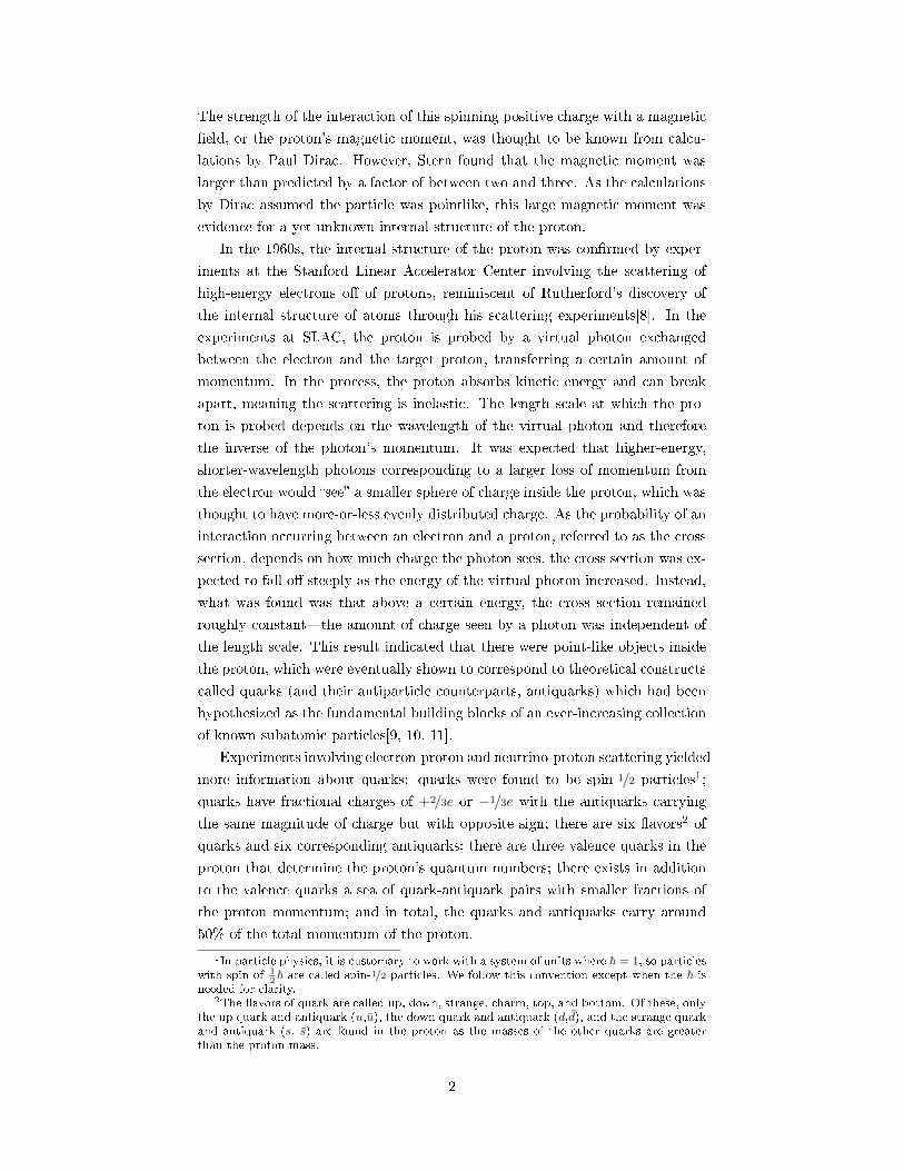
Figure 1.1: Cross sections for inelastic electron-proton scattering fromSLAC/MIT experiments[8]. The cross sections are normalized by the Mottscattering cross section, which describes the scattering of spin-1/2 particles o�of a heavy target, and are compared to expectations from elastic scattering.
3

The remaining 50% of the momentum of the proton comes from a massless
particle called the gluon[12]. The concept of the gluon was developed alongside
the quark models for subatomic structure; the gluon receives its name from the
fact that it carries the strong force that binds quarks together in the proton.
The nature of the interaction between quarks and gluons is central to this thesis
and will be discussed in more detail in the next section. For now, we will simply
state that the existence of the gluon was experimentally con�rmed by detecting
the experimental signature of a gluon being emitted by a quark produced via
e+e− annihilation, and the gluons were found to be spin-1 particles like photons
(which mediate the electromagnetic force) but in contrast to quarks.
1.2 The proton spin puzzle
We have arrived at a description of the proton, a composite spin-1/2 particle
comprised of irreducible spin-1/2 quarks and antiquarks as well as spin-1 glu-
ons, known collectively as partons. The momentum contributions of these con-
stituents was known from electron, muon, and neutrino scattering experiments,
but these experiments involved unpolarized beams and targets and could there-
fore not yield information about the alignment of the spins of the constituent
particles. Polarized beams and targets were being developed alongside the un-
polarized scattering experiments though, meaning the spin of the proton could
be studied in detail. It would be natural to assume that the proton's spin of 1/2
arises from the three valence quarks, with one of the spins oriented antiparallel
to the other two. Experimenters from multiple collaborations all found however
that the quarks inside the proton in total only carry about 25% of the proton's
spin: the proton spin crisis was born.
1.2.1 The pieces
We can easily identify the possible sources of the proton's spin of 1/2. The
quarks each carry intrinsic spin angular momentum of 1/2, which is to say if
one measures a single quark's spin with respect to the axis of the proton's spin
(which we call the z-axis), the result will be +1/2 if the quark's spin is parallel to
the proton's or −1/2 if it is antiparallel. The total contribution of the quark spins
is the di�erence between the numbers of parallel and antiparallel quark spins
times 1/2, which is represented as ∆Σ. The quarks can also have orbital angular
momentum with respect to the proton's spin axis, ∆Lq, from their motion in
the proton. The orbital angular momentum can only be integer multiples of ~,with the sign of the contribution again depending on the direction of the orbital
angular momentum vector compared to the proton's spin axis. Analogously, the
gluons can also contribute spin ∆G and orbital angular momentum ∆Lg, both
in integer multiples of ~. Then, representing the spin contributions from quarks
as ∆Σ and gluons as ∆G, we write a decomposition of the proton's longitudinal
4

spin, or the spin of the proton in the direction of its momentum3:
1
2=
1
2∆Σ + ∆G+ ∆Lq + ∆Lg. (1.1)
As mentioned above, the total quark contribution is fairly well-known from
lepton scattering experiments. The orbital angular momentum distributions are
under investigation via the measurement of transverse momentum dependent
(TMD) distribution functions. The gluon contribution ∆G is constrained to a
small degree in lepton scattering experiments through the interaction of gluons
with quarks (the gluons themselves do not interact directly with leptons as the
gluons have no electric or weak charge). The best constraints on ∆G currently
available are from polarized proton-proton collisions at RHIC. How we learn
about ∆G from polarized proton-proton collisions is the topic of the next section,
when we introduce some formalism and look at the scattering process in more
detail.
1.3 Accessing ∆G in polarized proton-proton
collisions
1.3.1 Quantum chromodynamics4
The theory of quantum chromodynamics (QCD) describes the strong force, in-
teractions between the quarks and gluons that comprise the proton. QCD de-
rives its name from the color charge carried by quarks or gluons. Quarks can
have one of three color charges, antiquarks have one of three corresponding anti-
color charges, and gluons carry one of eight color/anticolor combinations. That
the gluons carry the color charge di�erentiates the strong force from the electro-
magnetic force (where the corresponding force-carrying particle, the photon, is
chargeless) in very signi�cant ways. For example, gluons can temporarily �uctu-
ate into a quark-antiquark pair as photons can. This sea quark-antiquark pairs
popping into and out of existence tend to arrange themselves in the presence of
color charge (say, a quark) to e�ectively screen the amount of color charge visi-
ble outside of the region near the color charge. The result is that the strength of
a QCD interaction, represented by the strong interaction coupling constant αS ,
depends on the distance scale at which the interaction occurs. As mentioned
above, the scale is governed by the four-momentum transfer in the interaction,
which is denoted by q. The Lorentz-invariant quantity is the four-momentum
squared, which for a virtual particle is negative, so by convention we refer to
3This decomposition of the proton spin, proposed by Ja�e and Manohar, emphasizes theindividual partonic contributions to the proton spin. For more details regarding proton spindecompositions, see [13].
4We present a basic overview here. For textbooks with a more detailed introduction of thetopic, as well as some interesting historical backdrop, see [14, 15, 16].
5

the quantity Q2:
Q2 ≡ −q2 ≡ −(four −momentum transfer)2. (1.2)
Conceptually, as Q2 increases, one can peer deeper inside the cloud of quark-
antiquark pairs and see more of the unscreened color charge, so αs would be
expected to increase. This description does align with what we see in quantum
electrodynamics5, but in QCD, the gluons themselves carry a color charge and
an anticolor charge and arrange themselves in such a way that the e�ective
charge of the bare quark is spread out rather than screened. Recalling the
discussion of electron-proton scattering in section 1.1, for a charge spread out
over some volume, we expect the strength of an interaction with that charge to
decrease with increased Q2 and shorter length scales. So, in QCD, changes in Q2
have competing e�ects on αS : screening caused by quark-antiquark pairs and
antiscreening caused by gluons. Which of the two e�ects dominates depends on
the number of �avors of quark nf and the number of colors N (which determines
the number of gluons):
∂αs∂log(Q2)
= (2nf − 11N)α2s
2π. (1.3)
Since there are three colors and six �avors of quark, (2nf − 11N) is negative,
and the coupling constant αs decreases with increasing Q2 and increases with
decreasing Q2. The behavior of αs in both of these directions is important. The
behavior at large energies and short length-scales gives rise to the property of
QCD called asymptotic freedom. In this regime, quarks in the proton can be
approximated as free quarks, not interacting with other partons. This enables
calculations in QCD using perturbation theory (pQCD), wherein simpli�ed cal-
culations with analytic solutions are carried out, while correction terms to the
simpli�ed calculations come with factors of αs and become negligible because
of the smallness of αs. In the low-Q2 regime, on the other hand, αs becomes
large (∼ 1) for length scales on the order of the size of a nucleon. Here, the
correction terms from pQCD do not become negligible, so QCD calculations
describing interactions at this level are impossible. Furthermore, the strength
of the strong interaction actually increases with increasing distance. As a re-
sult, as two color charges separate, the potential energy between them grows to
the point where it becomes more energetically favorable for additional quark-
antiquark pairs to form, with all quarks, antiquarks, and gluons ending up in
color-neutral hadrons. There have been no detections of individual quarks, an-
tiquarks, or gluons�they obey a principle of QCD called con�nement, and the
process by which quarks, antiquarks, and gluons all end up as hadrons in the
�nal state is known as fragmentation6.
5Quantum electrodynamics is the quantum �eld theory of the electromagnetic force.6We also refer to the resulting cascade of particles in the direction of the fragmenting
parton as a jet.
6

In scattering experiments, the main quantity of interest is the rate of particle
production in the acceptance of the detectors. The rate depends on the speci�cs
of the experiment, such as the number of particles in the beam, the frequency at
which particles are incident on either a target or particles in another colliding
beam, and the spatial extent of the beam. Therefore, the quantity compared
between experiments is an intrinsic probability of particles colliding and inter-
acting in a certain way, and this probability is referred to as the cross section,
σ. The cross section is related to the rate of interactions:
σ =rate
L, (1.4)
where L is the luminosity, which, for a collider with beams a and b and numbers
of particles in the beams Na and Nb intersecting with a frequency f in a cross-
sectional area A, is given by
L =NaNbf
A. (1.5)
The cross section is generally measured over some period of time, where we
talk about an integrated luminosity and a total yield of interactions detected
Y , rather than a rate: ˆLdt =
Y
σ. (1.6)
1.3.2 Proton-proton collisions: parton distribution
functions, the partonic cross section, and
fragmentation functions
The framework of pQCD is suitable for calculating fundamental short-range
interactions between partons but not the complex long-range interactions in
hadrons where the e�ective αs is large. The QCD cross section of a high-energy
proton-proton collision where the quarks are considered asymptotically free can
be factorized into three components which can be analyzed separately and com-
bined into a �nal result. We schematically present such a collision in Figure 1.2.
The �rst non-calculable portion of the cross section parameterizes the internal
structure of the proton in the initial state in terms of parton distribution func-
tions (PDFs). These functions describe the number density of a given parton
(a d-quark or gluon, for example) with a certain fraction x of the total momen-
tum of the proton, described at a factorization scale7 µ2 which is generally set
to the squared four-momentum transfer in the interaction Q2 or the square of
the transverse momentum p2T of the �nal state hadron, as Q2 is not directly
7The dependence of the PDFs on the length scale can be thought of a reshu�ing of termsbetween the hard scattering component of the cross section and the PDF (or the fragmentationfunction). For example, a gluon radiated before the scattering by one of the interacting quarkscould be included in the pQCD calculation of the hard scattering cross section. Alternatively,the scale can be chosen such that the correction enters as a modi�cation of the PDF of theparton instead.
7

Figure 1.2: Schematic representation of an inelastic proton-proton scatteringevent[17]. A parton from each of the colliding protons (represented by threelines representing the three valence quarks) participates in the fundamentalhard scattering interaction, which is calculable in pQCD. Emerging from theinteraction are two partons that fragment into colorless particles. A hadron (inthis �gure, a pion denoted by π) from one of the fragmentation processes isdetected in the �nal state.
8
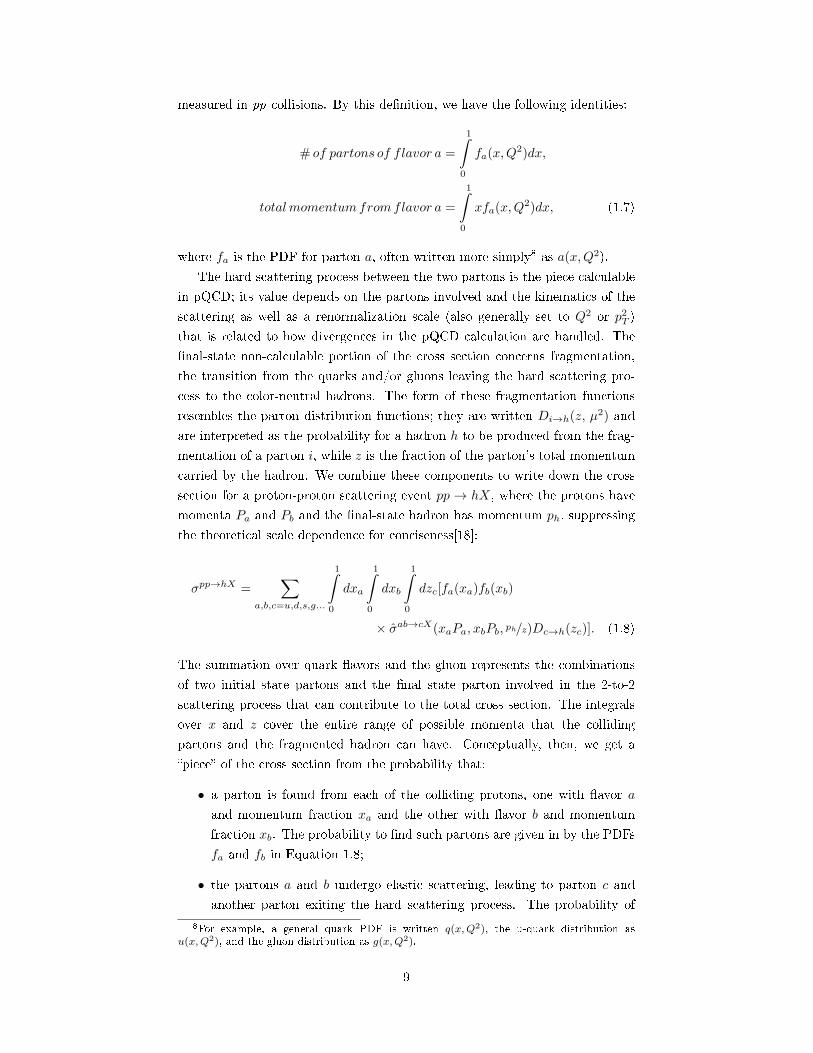
measured in pp collisions. By this de�nition, we have the following identities:
# of partons of flavor a =
1ˆ
0
fa(x,Q2)dx,
totalmomentumfromflavor a =
1ˆ
0
xfa(x,Q2)dx, (1.7)
where fa is the PDF for parton a, often written more simply8 as a(x,Q2).
The hard scattering process between the two partons is the piece calculable
in pQCD; its value depends on the partons involved and the kinematics of the
scattering as well as a renormalization scale (also generally set to Q2 or p2T )
that is related to how divergences in the pQCD calculation are handled. The
�nal-state non-calculable portion of the cross section concerns fragmentation,
the transition from the quarks and/or gluons leaving the hard scattering pro-
cess to the color-neutral hadrons. The form of these fragmentation functions
resembles the parton distribution functions; they are written Di→h(z, µ2) and
are interpreted as the probability for a hadron h to be produced from the frag-
mentation of a parton i, while z is the fraction of the parton's total momentum
carried by the hadron. We combine these components to write down the cross
section for a proton-proton scattering event pp → hX, where the protons have
momenta Pa and Pb and the �nal-state hadron has momentum ph, suppressing
the theoretical scale dependence for conciseness[18]:
σpp→hX =∑
a,b,c=u,d,s,g...
1ˆ
0
dxa
1ˆ
0
dxb
1ˆ
0
dzc[fa(xa)fb(xb)
× σab→cX(xaPa, xbPb, ph/z)Dc→h(zc)]. (1.8)
The summation over quark �avors and the gluon represents the combinations
of two initial state partons and the �nal state parton involved in the 2-to-2
scattering process that can contribute to the total cross section. The integrals
over x and z cover the entire range of possible momenta that the colliding
partons and the fragmented hadron can have. Conceptually, then, we get a
�piece� of the cross section from the probability that:
• a parton is found from each of the colliding protons, one with �avor a
and momentum fraction xa and the other with �avor b and momentum
fraction xb. The probability to �nd such partons are given in by the PDFs
fa and fb in Equation 1.8;
• the partons a and b undergo elastic scattering, leading to parton c and
another parton exiting the hard scattering process. The probability of
8For example, a general quark PDF is written q(x,Q2), the u-quark distribution asu(x,Q2), and the gluon distribution as g(x,Q2).
9

this interaction is given by the parton-level cross section σ;
• and the parton c, a product of the hard scattering interaction, fragments
into the hadron h with a probability dependent on the momentum of the
hadron: Dc→h(zc).
1.3.3 Polarized proton-proton collisions
We can generalize Equation 1.8, which makes no reference to the polarization of
the protons or the quarks and gluons, to the case of polarized pp collisions. As
mentioned in section 1.1, the polarization measured along any axis for a spin-1/2
particle is ± 12~. Consequently, quarks and gluons in the proton can be found
with either the same or opposite helicity as the proton. The unpolarized parton
distribution functions f(x,Q2) are a sum of contributions of the aligned (+)
and antialigned (−) partons:
f(x,Q2) = f+(x,Q2) + f−(x,Q2), (1.9)
and the di�erence of the spin-separated PDFs we call the helicity parton distri-
bution functions:
∆f(x,Q2) = f+(x,Q2)− f−(x,Q2). (1.10)
The total spin contributed to the proton from a particular �avor of quark or a
gluon can be found by taking the product of the parton's spin with the integral
of the helicity distribution over all x:
∆Σ(Q2) =1
2
∑a=q,q
1ˆ
0
∆fa(x,Q2)dx,
∆G(x,Q2) =
1ˆ
0
∆g(x,Q2)dx, (1.11)
where ∆Σ is the contribution from all �avors of quarks and antiquarks.
With polarized partons undergoing the hard scattering process, helicity-
conservation e�ects come into play, and σab→cX has a di�erent value depending
on whether the two colliding partons have the same or opposite helicity (++
or +− referring to the sign of the helicity of the two partons). Similarly to the
helicity PDFs, we have a spin-dependent parton-level cross section:
σab→cX = (σab→cX)++ + (σab→cX)+−,
∆σab→cX = (σab→cX)++ − (σab→cX)+−. (1.12)
For our purposes, we only consider fragmentation functions from unpolarized
quarks, meaning the fragmentation function Dc→h(z) is the same in the unpo-
10

larized and helicity-dependent cross sections.
With the above de�nitions in mind, we now can see how the gluon helicity
distribution, ∆g(x,Q2), is accessed at RHIC. We formulate a cross section asym-
metry that is the di�erence between the cross sections for protons with the same
helicity versus the opposite helicity. The expression looks similar in form to the
unpolarized cross section of Equation 1.8, but the PDFs and parton-level cross
section have been replaced by their helicity-dependent analogues. Measuring
a di�erence in cross sections and normalizing by the unpolarized cross section
greatly simpli�es the analysis because detector acceptances and e�ciencies are
assumed to be independent of the spin states of the interacting protons, meaning
these e�ects cancel out in the ratio. The double longitudinal spin asymmetry
ALL is de�ned as
ALL =σ++ − σ+−
σ++ + σ+− =∆σ
σ, (1.13)
where the helicity superscripts now refer to the helicities of the colliding protons
rather than the partons and ∆σ is the cross section with the helicity-dependent
parton distribution functions and partonic cross section substituted for their
unpolarized counterparts from Equation 1.8:
∆σpp→hX =∑
a,b,c=u,d,s,g...
1ˆ
0
dxa
1ˆ
0
dxb
1ˆ
0
dzc[∆fa(xa)∆fb(xb)
×∆σab→cX(xaPa, xbPb, ph/z)Dc→h(zc)]. (1.14)
The asymmetry ALL is sensitive to ∆q(x)q(x)
∆g(x)g(x) through quark-gluon scattering
processes and ∆g(x)g(x)
∆g(x)g(x) through gluon-gluon scattering. The partonic cross
section asymmetry aLL modulates the strength of the overall asymmetry to the
helicity PDFs and can be thought of as an analyzing power. The partonic cross
section is a function of the center-of-mass scattering angle and the types of
partons involved in the scattering. The value of aLL for various processes from
pQCD calculations is shown in Figure 1.3.
In terms of measuring the asymmetry, we start with Equation 1.13 and
consider the σ++(+−) terms. We have a relation between cross sections and the
particle yield N (e.g. number of pions, electrons, scaler counts), given by
σ =N
L, (1.15)
where the N must be corrected for detector e�ciency and acceptance e�ects:
N =Nmeasεdetεacc
. (1.16)
We assume that the e�ciencies are the same for same-sign and opposite-sign
helicity crossings, so they factor out and cancel in the ratio in Equation 1.13.
11
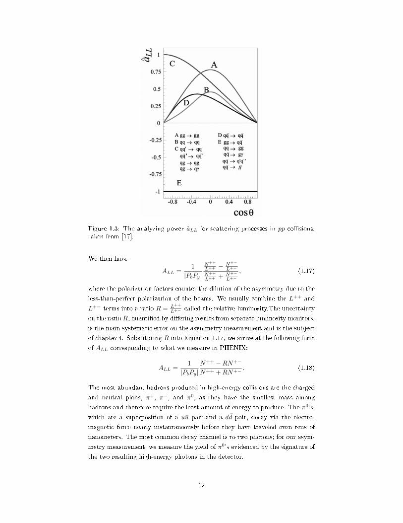
Figure 1.3: The analyzing power aLL for scattering processes in pp collisions,taken from [17].
We then have
ALL =1
|PbPy|
N++
L++ − N+−
L+−
N++
L++ + N+−
L+−
, (1.17)
where the polarization factors counter the dilution of the asymmetry due to the
less-than-perfect polarization of the beams. We usually combine the L++ and
L+− terms into a ratio R = L++
L+− called the relative luminosity.The uncertainty
on the ratio R, quanti�ed by di�ering results from separate luminosity monitors,
is the main systematic error on the asymmetry measurement and is the subject
of chapter 4. Substituting R into Equation 1.17, we arrive at the following form
of ALL corresponding to what we measure in PHENIX:
ALL =1
|PbPy|N++ −RN+−
N++ +RN+− . (1.18)
The most abundant hadrons produced in high-energy collisions are the charged
and neutral pions, π+, π−, and π0, as they have the smallest mass among
hadrons and therefore require the least amount of energy to produce. The π0's,
which are a superposition of a uu pair and a dd pair, decay via the electro-
magnetic force nearly instantaneously before they have traveled even tens of
nanometers. The most common decay channel is to two photons; for our asym-
metry measurement, we measure the yield of π0's evidenced by the signature of
the two resulting high-energy photons in the detector.
12

1.4 Description of kinematics
In a hard scattering QCD interaction between protons, two partons collinear
with the protons with momenta x1P1 and x2P2 interact through the exchange
of a gluon9 with squared four=momentum q2 = −Q2. The two partons exiting
the hard interaction fragment, and a hadron deposits energy in a detector. We
characterize the hadron by its energy, its transverse momentum pT (transverse
to the beam axis) de�ned as
pT =√p2x + p2
y, (1.19)
and its pseudorapidity η, de�ned in terms of the angle θ between the hadron
and the beam axis as
η = −ln[tan(θ
2)]. (1.20)
The pseudorapidity is 0 for particles scattered at a right angle to the beam axis,
while η →∞ along the positive direction of the beam axis and η → −∞ in the
backward direction.
1.5 Global QCD analyses
In order to extract information about the helicity PDFs through asymmetry
measurements in pp, the other components of the polarized and unpolarized
cross sections need to be constrained. The universality of the factorized compo-
nents of cross sections is assumed, meaning those components are independent
of the type of experiment in which they arise. In other words, a parton distribu-
tion or fragmentation function measured in a lepton scattering experiment will
be the same as one found from a proton-proton collision and so on. Di�erent
types of experiment are better suited to provide di�erent pieces of information.
For instance, electron-positron colliders have simple initial states with no par-
ton distribution functions to worry about, but the e+e− annihilation produces
quark-antiquark pairs that fragment into hadrons in the �nal state. Studying
the production rates of hadrons with a range of momenta allows for precise
determination of fragmentation functions. Also, recall from section 1.1 that
lepton-proton scattering experiments have placed strong constraints on the un-
polarized PDFs. In general, theorists perform �ts to data from many di�erent
experiments at di�erent center of mass energies and Q2 to determine the long-
range interactions not calculable in pQCD. This type of analysis is known as a
global analysis.
9In the vast majority of cases, the partons interact via the strong force, exchanging a gluon.In a small fraction of collisions, the partons can exchange a W or Z boson (the force carriersof the weak force) or a photon (the force carrier of the electromagnetic force).
13
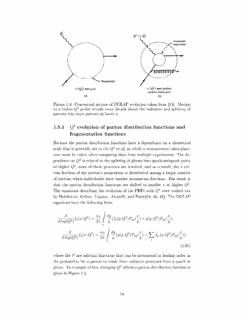
Figure 1.4: Conceptual picture of DGLAP evolution taken from [15]. Movingto a higher-Q2 probe reveals more details about the radiation and splitting ofpartons into more partons at lower x.
1.5.1 Q2 evolution of parton distribution functions and
fragmentation functions
Because the parton distribution functions have a dependence on a theoretical
scale that is generally set to the Q2 or p2T at which a measurement takes place,
care must be taken when comparing data from multiple experiments. The de-
pendence on Q2 is related to the splitting of gluons into quark-antiquark pairs;
at higher Q2, more of these processes are resolved, and as a result, the a cer-
tain fraction of the proton's momentum is distributed among a larger number
of partons which individually have smaller momentum fractions. The result is
that the parton distribution functions are shifted to smaller x at higher Q2.
The equations describing the evolution of the PDFs with Q2 were worked out
by Dokshitzer, Gribov, Lipatov, Altarelli, and Parisi[19, 20, 21]. The DGLAP
equations have the following form:
d
d log(Q2)fq(x,Q
2) =αS2π
1ˆ
x
dy
y(fq(y,Q
2)Pqq(x
y) + g(y,Q2)Pqg(
x
y),
d
d log(Q2)fg(x,Q
2) =αS2π
1ˆ
x
dy
y(g(y,Q2)Pgg(
x
y) +
∑i
fqi(y,Q2)Pgq(
x
y)),
(1.21)
where the P are splitting functions that can be interpreted at leading order as
the probability for a parton to result from radiative processes from a quark or
gluon. An example of how changing Q2 a�ects a parton distribution function is
given in Figure 1.5.
14
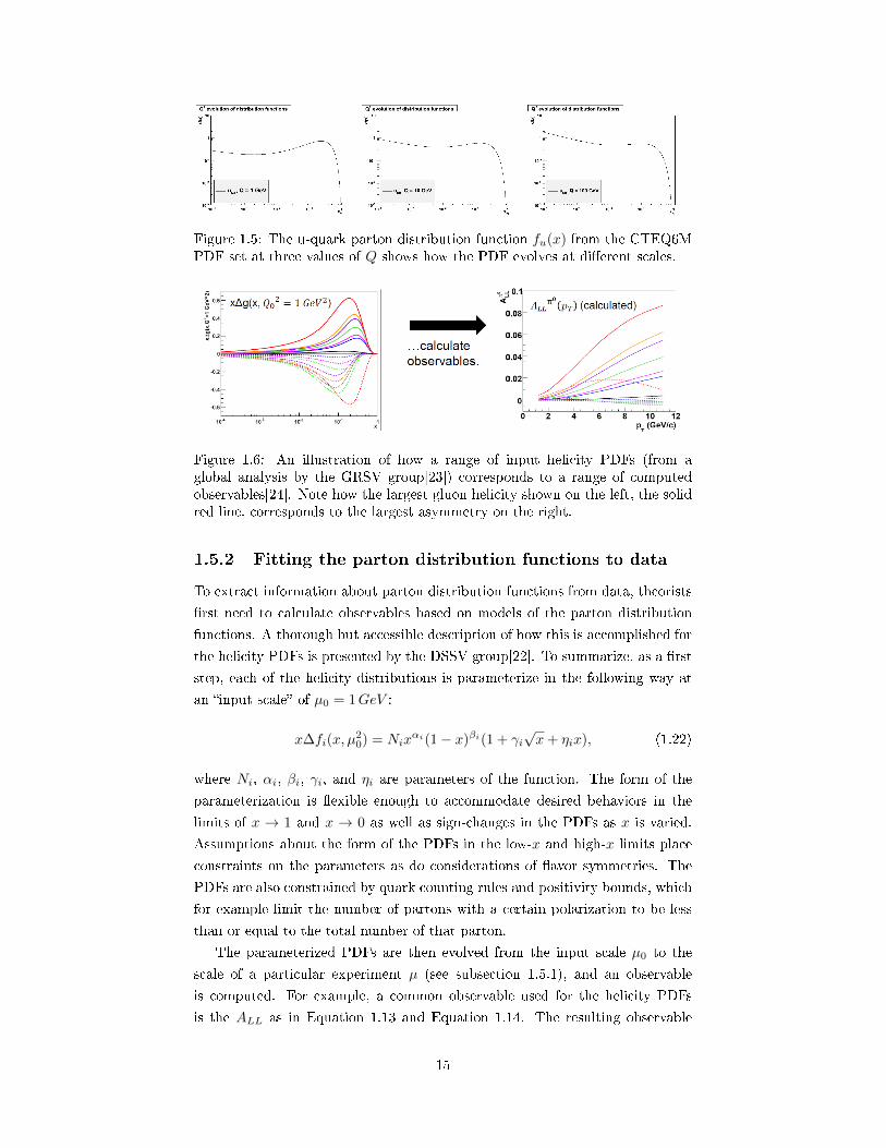
Figure 1.5: The u-quark parton distribution function fu(x) from the CTEQ6MPDF set at three values of Q shows how the PDF evolves at di�erent scales.
Figure 1.6: An illustration of how a range of input helicity PDFs (from aglobal analysis by the GRSV group[23]) corresponds to a range of computedobservables[24]. Note how the largest gluon helicity shown on the left, the solidred line, corresponds to the largest asymmetry on the right.
1.5.2 Fitting the parton distribution functions to data
To extract information about parton distribution functions from data, theorists
�rst need to calculate observables based on models of the parton distribution
functions. A thorough but accessible description of how this is accomplished for
the helicity PDFs is presented by the DSSV group[22]. To summarize, as a �rst
step, each of the helicity distributions is parameterize in the following way at
an �input scale� of µ0 = 1GeV :
x∆fi(x, µ20) = Nix
αi(1− x)βi(1 + γi√x+ ηix), (1.22)
where Ni, αi, βi, γi, and ηi are parameters of the function. The form of the
parameterization is �exible enough to accommodate desired behaviors in the
limits of x → 1 and x → 0 as well as sign-changes in the PDFs as x is varied.
Assumptions about the form of the PDFs in the low-x and high-x limits place
constraints on the parameters as do considerations of �avor symmetries. The
PDFs are also constrained by quark counting rules and positivity bounds, which
for example limit the number of partons with a certain polarization to be less
than or equal to the total number of that parton.
The parameterized PDFs are then evolved from the input scale µ0 to the
scale of a particular experiment µ (see subsection 1.5.1), and an observable
is computed. For example, a common observable used for the helicity PDFs
is the ALL as in Equation 1.13 and Equation 1.14. The resulting observable
15

is compared to the actual data points provided by the experiment, and the
parameters of Equation 1.22 are varied to minimize the χ2. Uncertainty bands
on the helicity PDFs are mapped out by varying the �t parameters until the
χ2 values reach some distance from the minimum; the DSSV group and other
analyzers of global QCD data have found that uncertainty bands that cover∆χ2
χ2 = 2% tend to encompass the �best �t� PDFs resulting from successive
iterations of the global analyses.
1.5.3 Current knowledge of parton distribution functions
While DIS experiments have been successful in determining the polarized parton
distributions for quarks, they are not as useful in constraining ∆g(x,Q2). As
mentioned above, the only constraints placed on ∆g(x,Q2) from inclusive DIS
arise from the DGLAP evolution equations which describe the interdependence
of ∆q(x,Q2) and ∆g(x,Q2) as Q2 varies. Polarized experiments have covered a
fairly limited range ofQ2 though, meaning ∆g(x,Q2) is only weakly constrained.
Under the assumption of universality, theorists and experimentalists can at-
tempt to simultaneously �t PDFs or polarized PDFs to cross sections measured
at various DIS and proton-proton scattering experiments. The CTEQ (Coordi-
nated Theoretical-Experimental Project on QCD) collaboration has performed
such a global �t for unpolarized PDFs, most recently in collaboration with Jef-
ferson Lab in 2013[25], while de Florian, Sassot, Stratmann, and Vogelsang
(DSSV) continually work on �ts for polarized PDFs[22]. Presently, the unpolar-
ized PDFs and the total u− and d-quark polarized distributions are well-known,
whereas the polarized sea-quark PDFs are less well-constrained, and the polar-
ized gluon PDF is weakly constrained, particularly at high and low x (see Fig.
1 and Fig. 2). The PHENIX experiment at RHIC is working towards measure-
ments that will speci�cally help to constrain the polarized sea-quark and gluon
PDFs.
Data from the RHIC experiments STAR and PHENIX provides the strongest
constraints on the gluon polarization thus far. While lepton-hadron scattering
experiments have provided strong constraints on the quark distribution func-
tions on account of the direct (leading order in pQCD) interactions between lep-
tons and quarks, these experiments are only sensitive to the electrically neutral
gluons through DGLAP evolution of the quark distribution functions. Addition-
ally, before 2009, measurements of ALL in PHENIX and RHIC were con�ned
to �nal states detected in a limited range of scattering angle near θ = 90◦. As
we will discuss in detail later on, this means that the polarizations of gluons is
unconstrained at low momentum fractions, where the total number of gluons is
very large compared to the other parton densities. Measuring ALL at kinemat-
ics that provide information on the gluon helicity for low-x is the focus of this
measurement.
16

(a) PDFs from CJ12 global �t, from [25];note the factor of x on the y-axis and the1/10 factor applied to the gluon distribution.
(b) Polarized PDFs from global �t byDSSV from 2009[22]; note the factor of xon the y-axes.
Figure 1.7: Parton distribution functions extracted from global QCD data.
17

Chapter 2
Experimental overview
2.1 The Relativistic Heavy Ion Collider
PHENIX is located at the Relativistic Heavy Ion Collider (RHIC) at Brookhaven
National Laboratory on Long Island, NY[26, 27] . The construction of the col-
lider along with PHENIX and three other experiments, called STAR, BRAHMS,
and PHOBOS, was completed in 1999. Of these experiments, the multi-purpose
experiments STAR and PHENIX are the two that remain operational; a Drell-
Yan experiment called AnDY ran at the BRAHMS interaction point from 2011-
2013. The purpose of RHIC was chie�y to collide heavy ions to reach the
high energy densities required to observe a predicted phase of matter called the
quark-gluon plasma. The existing linear accelerator at BNL had the ability to
accelerate polarized protons however, and advances in spin-rotator technology
(particularly in collaboration with the RIKEN research institute in Japan) al-
lowed the plans for RHIC to extend to studying the spin structure of the proton
as the world's only polarized proton-proton (pp) collider.
Since the �rst physics running in 2000, RHIC has demonstrated impressive
�exibility both in heavy ion and polarized proton running. For the heavy ion
programs, RHIC has collided deuterons as well as copper, gold, uranium, and
aluminum ions at energies of 3.85GeV/nucleon to 100GeV/nucleon. To study
spin physics, RHIC has collided transversely and longitudinally polarized pro-
tons at center-of-mass energies up to√s = 510GeV with polarizations above
50%, and this year for the �rst time, polarized protons have been collided with
heavy ions at energies of 100GeV/nucleon[29].
2.1.1 Accelerator chain
We provide a brief summary here of the production, acceleration, storage, and
collision of polarized protons at RHIC; a more detailed explanation can be found
in [30]. On the order of 1012 polarized H− ions are produced by an optically
pumped polarized ion source. The H− ions are accelerated to an energy of
200MeV by a linear accelerator and are stripped of their electrons, leaving po-
larized protons to be injected into the Alternating Gradient Synchrotron (AGS)
Booster. The AGS Booster accelerates the protons to 1.5GeV and delivers
them to the larger Alternating Gradient Synchrotron, where the protons reach
18

Figure 2.1: An overview of the RHIC/AGS accelerator complex at BrookhavenNational Laboratory[28].
energies of 25GeV . Finally, the bunch of protons, having at this point closer to
1011 protons, is injected into one of two storage rings in RHIC with a circumfer-
ence of 3.8 km. The two rings store counter-rotating beams, called the blue and
yellow beams, which each hold up to 120 bunches of ions separated by 106ns,
and all bunches can be �lled in about 10 minutes. There are nine consecutive
un�lled buckets at the end of the 120 crossings referred to as the abort gap that
allows kicker magnets the time to ramp up to de�ect the beam into beam dumps
when the beams need to be aborted. The luminosity and pro�le of bunches in
the beams are monitored by a system of wall current monitors. These monitors
measure voltage from an image current generated on a conducting pipe by the
ions in the beam. This current is forced across a resistive gap allowing a voltage
to be read out; every �ve minutes, the voltage is sampled for approximately
12µs at intervals of 0.05ns, giving a picture of the charge in both beams at
every point around the ring as the duration of the sampling corresponds to the
revolution period of the protons.
The bunches from the two beams are brought into collision via steering mag-
nets and focusing magnets at up to four collision points; the width of the bunches
in the longitudinal direction is such that nearly all collisions between protons in
the two bunches take place in a range of ±150 cm from the nominal interaction
point. Even with 100 billion protons in each of the intersecting bunches, though,
collisions between protons are extremely rare. For each crossing of bunches, we
see on the order of one inelastic pp collision.
One set of injected bunches in each beam is allowed to remain in the beam
for a number of hours (in Run 11 generally not more than six hours) until the
19

luminosity and polarization deteriorate past the point of usefulness at which
point the beams are dumped. The period of running from one store of protons
or ions is called a �ll. PHENIX further divides the �ll into data-taking segments
of up to an hour-long called runs (not to be confused with the Run, as in Run
11, which refers to a year of data taking). Restarting the data acquisition
system in PHENIX more frequently allows the shift crew to debug the detectors
and electronics systems, preventing problems from compromising an entire �ll's
worth of data.
2.1.2 Spin rotators, spin patterns, and Siberian snakes
Helical dipole magnets are employed at RHIC in order to manipulate the di-
rection of the spin of the polarized protons. This capability is needed for
two purposes�to deliver transversely or longitudinally polarized protons to
PHENIX and STAR and to maintain a high level of polarization in the pro-
ton bunches. The spin rotators are located on either side of the PHENIX and
STAR experiments and change the polarization direction of the protons, which
circulate with their spins transversely up or down with respect to their momen-
tum direction, to a positive or negative helicity state. For each of the ≈ 107
�lled bunches, the blue beam bunch and yellow beam bunch together can have
one of four helicity con�gurations: the blue and yellow bunches can both have
either positive or negative helicity, or the blue bunch can have positive helic-
ity and the yellow bunch negative, or vice versa. For analyses of double spin
asymmetries, yields from the same-sign (both positive or both negative) and
opposite-sign (one positive, one negative) bunches are grouped together. To
avoid time- or crossing-dependent e�ects that cause systematic di�erences be-
tween the helicity con�gurations, the helicities of the blue and yellow bunches
are organized in patterns consisting of repeating groups of 8 crossings that sam-
ple each helicity con�guration twice. In Run 11, four such spin patterns were
used. For two patterns, the pattern of same-sign and opposite-sign crossings,
denoted by S and O, is �SOOSOSSO� beginning with the �rst crossing, labeled
crossing 0. One of the two patterns has all helicities multiplied by −1 relative to
the other. Similarly, the other two spin patterns are arranged as �OSSOSOOS,�
again beginning with crossing 0 and having a relative sign di�erence of −1 in
the bunch helicities.
The purpose of the other group of helical dipole magnets in the accelera-
tors, the Siberian snakes, is to counter the e�ect of depolarization resonances
while the protons are being accelerated or stored. The depolarization resonances
occur due to disturbances to the proton's spin from focusing magnets or imper-
fections in the magnetic �elds that maintain the proton's vertical polarization.
The disturbances are ampli�ed when they occur at the same frequency as the
precession of the proton's spin. The Siberian snakes in RHIC �ip the spin of the
protons by 180◦ twice for each orbit in RHIC, with the result that the e�ect of
20

destabilizing magnetic �elds on the protons' spins cancel out during the course
of a complete orbit. The AGS also uses partial Siberian snakes to avoid the
depolarizing resonances.
2.1.3 RHIC Polarimetry
The polarization of the beams in RHIC is measured at the 12 o'clock position in
the ring by two subsystems, the proton-carbon (pC) and the hydrogen jet (H-
jet) polarimeters. Both measure left-right asymmetries in the elastic scattering
of the polarized protons in the beam o� of a target. The protons in the H-
jet target are polarized, allowing an absolute polarization of the beam to be
determined, but the rate of interactions between the beam protons and the dilute
gas jet is small resulting in large statistical uncertainties. The pC polarimetry
measurement is complementary in the sense that it measures a very high rate
of interactions, allowing for quick measurements that can determine the change
in beam polarization over time. However, the carbon target is unpolarized, and
the polarization measurements from the pC system need to be calibrated with
the results from the H-jet polarimeter.
Additionally, there are detectors along the beam pipe at experiments at
RHIC known as Zero Degree Calorimeters that monitor the luminosity of the
beams by detecting neutrons from di�ractive interactions between protons. In
PHENIX, an array of scintillator strips called the Shower Maximum Detector
determines the position of the neutrons with the resolution needed to measure
a left-right asymmetry. By analyzing this asymmetry, a local polarization mea-
surement can be done that con�rms that the colliding protons are successfully
rotated to longitudinal polarization for collisions in PHENIX during longitudi-
nal pp running.
2.2 The PHENIX detector
The array of detectors that comprise the PHENIX experiment are located at 8
o'clock on the RHIC ring[31]. PHENIX consists of groups of detectors covering
sections around the collision point and serving various purposes:
• The central arm is comprised of two spectrometers that each cover |η| <0.35 and 90◦ in φ. The central arm provides tracking and calorimetry.
• The muon arm covers 1.2 < |η| < 2.4 and is used for identifying, tracking,
and triggering on high-pT muons.
• The Muon Piston Calorimeter (MPC) sits in a hole around the beam pipe
in the muon arms. It covers 3.1 < |η| < 3.9 and 2π azimuthally and was
designed to study nucleon structure at low momentum fraction x.
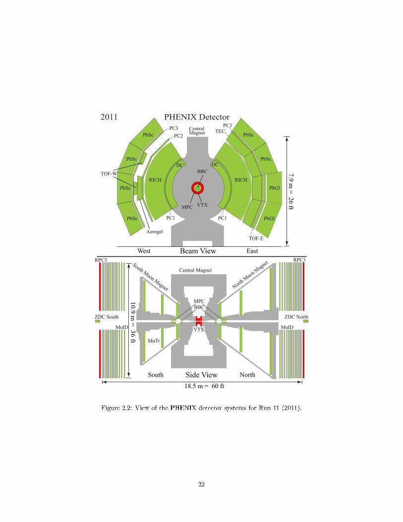
• There are also detectors used for event characterization; the Beam-Beam
Counter (BBC), a pair of detectors encircling the beam pipe at ±144 cm
21
West
South Side View
Beam View
PHENIX Detector2011
North
East
MuTr
MuID
RPC3
MuID
RPC3
MPC
BBC
VTX
PbSc PbSc
PbSc PbSc
PbSc PbGl
PbSc PbGl
TOF-E
PC1 PC1
PC3PC2
Central Magnet
CentralMagnet
North M
uon MagnetSouth Muon Magnet
TECPC3
BBC
VTX
MPC
BB
RICH RICH
DC DC
ZDC NorthZDC South
Aerogel
TOF-W 7.9 m = 26 ft
10.9 m = 36 ft
18.5 m = 60 ft
Figure 2.2: View of the PHENIX detector systems for Run 11 (2011).
22
which PHENIX uses as a minimum bias trigger for inelastic pp collisions,
and the Zero Degree Calorimeter, which sits on the beam axis at ±18m
and monitors the luminosity by detecting neutrons from di�ractive pp
interactions.
For the purposes of our measurement, we only include data collected by the
MPC, BBC, and ZDC; we brie�y introduce the BBC and the ZDC here, while
the MPC will be covered in more detail below.
Coordinates We will also refer to coordinates with respect to PHENIX in
this thesis. For reference, the x-axis and y-axis are perpendicular to the beam,
with the x-axis being horizontal and the y-axis vertical. The z-axis is along the
beam, with z = 0 cm being the center of PHENIX. We refer to the polar angle,
or the angle between a vector and the beam axis, as θ, while the azimuthal angle
around the beam axis is referred to as φ.
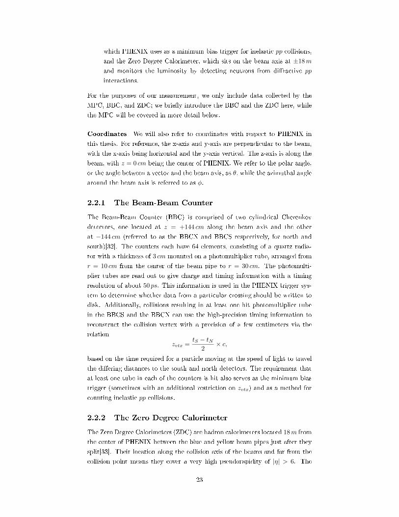
2.2.1 The Beam-Beam Counter
The Beam-Beam Counter (BBC) is comprised of two cylindrical Cherenkov
detectors, one located at z = +144 cm along the beam axis and the other
at −144 cm (referred to as the BBCN and BBCS respectively, for north and
south)[32]. The counters each have 64 elements, consisting of a quartz radia-
tor with a thickness of 3 cm mounted on a photomultiplier tube, arranged from
r = 10 cm from the center of the beam pipe to r = 30 cm. The photomulti-
plier tubes are read out to give charge and timing information with a timing
resolution of about 50 ps. This information is used in the PHENIX trigger sys-
tem to determine whether data from a particular crossing should be written to
disk. Additionally, collisions resulting in at least one hit photomultiplier tube
in the BBCS and the BBCN can use the high-precision timing information to
reconstruct the collision vertex with a precision of a few centimeters via the
relation
zvtx =tS − tN
2× c,
based on the time required for a particle moving at the speed of light to travel
the di�ering distances to the south and north detectors. The requirement that
at least one tube in each of the counters is hit also serves as the minimum bias
trigger (sometimes with an additional restriction on zvtx) and as a method for
counting inelastic pp collisions.
2.2.2 The Zero Degree Calorimeter
The Zero Degree Calorimeters (ZDC) are hadron calorimeters located 18m from
the center of PHENIX between the blue and yellow beam pipes just after they
split[33]. Their location along the collision axis of the beams and far from the
collision point means they cover a very high pseudorapidity of |η| > 6. The
23

calorimeters are designed to detect low pT neutral particles emerging from pp
interactions, and coincidences between the north and south arms are used as a
luminosity monitor similar to the BBC, but with poorer timing (and therefore
zvtx) resolution. In between the �rst two layers of the calorimeters is the Shower
Maximum Detector, which as mentioned in subsection 2.1.3 allows su�cient po-
sition resolution to measure an asymmetry in the neutron yields as an indicator
of the beam polarizations.
2.2.3 Data acquisition (DAQ) system
The data acquisition system at PHENIX[34] has to be able to write a large
volume of data, quickly sift through an even larger amount of data, and com-
bine information from all of the detector components in PHENIX in order to
function properly. Each detector system has a front-end electronics module
(FEM) that digitizes the raw analog signals from the detector and temporarily
stores the data in a bu�er to wait for a trigger decision indicating whether the
data should be written out. The FEMs also send the data needed to determine
whether or not an event is �interesting� to a system called the Local Level-1
(LL1), which processes the data and passes along an �accept� signal (a trigger)
if programmable conditions are met. The Global Level-1 (GL1) system looks at
the output from the various LL1 systems and makes a decision about whether
or not data from a crossing should be recorded. In the event that the GL1's
conditions are met and the DAQ is not in a busy state, it signals the FEMs
via each system's Granule Timing Module (which also ensures that the various
detectors are synchronized by passing along a beam clock timing signal). At
this point, the FEMs send their data to a Data Collection Module (DCM) which
feeds into a Sub-Event Bu�er and �nally an Assembly Trigger Processor. These
last two systems handle the combining of data from the various subsystems
into �events,� any higher-level trigger decisions needed, and the sending of the
complete events' data to hard disks.
From the prospective of a data analyzer in PHENIX, the �nal product is a
set of Data Summary Tables, or DSTs, that are the result of production software
running over raw data �les. The DST �les contain all of the data relevant for
an analysis for a particular detector subsystem and class of event in a human-
understandable format. For example, such a �le for the MPC contains (among
other things) the location and energies for hits in the detector from events meet-
ing a speci�ed trigger condition. The majority of the analysis is performed using
a framework of C++ libraries called ROOT[35]. ROOT provides various data
structures that are generally useful to particle physics analysis; in particular,
data can be organized in a tree structure that tracks the link between all data
common to a certain event. This allows analysis code to be written to compre-
hensively process a single event while ROOT and a PHENIX-speci�c interface to
the DSTs called Fun4All handle the running of each event through the analysis
24

code.
2.2.4 Scaler boards
The DAQ system includes additional components called scaler boards, which
count the number of triggers that occur over the course of the run. The scaler
boards preserve information that would normally be lost due to limits on the
speed of writing data to disk. Certain triggers �re at a rate at which writing out
data for each incidence would be impossible. Therefore, only a small, randomly-
sampled fraction of events selected by these triggers can be fully written out.
The scaler boards at least allow us to track how often the trigger conditions in
the detector systems were met.
There are three sets of scaler boards in PHENIX that we use in this analysis:
the GL1 scalers, the GL1p scalers, and the STAR scalers[36]. The GL1p and
STAR scalers each count triggers on a crossing-by-crossing basis, allowing for
the relative luminosity between bunches of di�erent helicity con�gurations to
be determined. The GL1p board can scale four trigger inputs. In Run 11, these
were the BBCLL1(>0 tubes) trigger, which requires a hit in the BBCS and the
BBCN as well as |zvtx| < 30 cm; the BBCnarrow trigger, which again requires
a coincidence between the BBCS and BBCN but has a stricter vertex cut of
|zvtx| < 15 cm; the ZDCwide trigger, which requires a coincidence between the
north and south arms of the ZDC and |zvtx| < 150 cm; and the ZDCnarrow
trigger, which requires a ZDC coincidence and |zvtx| < 30 cm. The STAR
scalers include these four triggers as well as a BBCwide trigger with no vertex
cut and a clock trigger which counts the number of bunch crossings during a
run. The STAR scalers also store information on whether the DAQ was available
to write data for particular crossings, allowing us to distinguish between �raw�
(all crossings) and �live� crossings. The GL1 boards scale the total number of
triggers integrated over all crossings. We use the GL1 as a cross-check to the
results we see from the GL1p and the STAR scalers. The scaler boards play a
central role in the relative luminosity analysis discussed in detail in chapter 4.
2.3 The Muon Piston Calorimeter
The Muon Piston Calorimeter (MPC) is a forward calorimeter upgrade to
PHENIX designed, constructed, and installed between 2005 and 2008[37]. Uni-
versity of Illinois scientists1 led the proposal, development, and construction of
the detector, which had the scienti�c goals of measuring transverse single spin
asymmetries, measuring the double longitudinal spin asymmetry at low-x, and
looking for signs of low-x gluons reaching a saturation point (i.e. the Color
Glass Condensate) in heavy ion collisions[38].
1Professor Matthias Grosse Perdekamp, post-doctoral researcher Mickey Chiu, and gradu-ate students John Koster and Beau Meredith.
25

(a) CAD drawing of one arm of the MuonPiston Calorimeter.
(b) One arm of the MPC in its positionaround the beam pipe in the muon piston.
Figure 2.3: The Muon Piston Calorimeter
There were very limited options for placement of the MPC in PHENIX, and
the design of the detector re�ects those limitations. The detectors are restricted
in size because they sit in a hole between the muon arm magnet yoke and
the beam pipe; the hole has an a diameter of 45 cm, while beam pipe-related
structures provide an inner diameter minimum of 6.5 inches in the south arm
and 4.62 inches in the north arm. These considerations most obviously constrain
the geometric acceptance of the MPC, but they also impact the choice of the
crystal used for the calorimetry. As we will discuss below, photons and electrons
incident on the calorimeter initiate showers of particles with a lateral extent
that depends on the material used in the calorimeter. In order to best be able
to resolve multiple hits2 in such a small space, we need to use crystals that
limit the lateral development of showers as much as possible. The measure of
this property for calorimeter materials is the Molière radius, and lead tungstate
(PbWO4) crystals were ultimately chosen for their small Molière radius, which is
of roughly the same size as the transverse size of the crystals. The dimensions of
the crystals are 2.2×2.2×18 cm3, where the �rst two dimensions are transverse
to the beam direction and the third is in the direction of the beam, and the
MPCS contains 196 such crystals while the MPCN has 220.
The scintillation light generated by showers in the crystals needs to be
quickly converted into an ampli�ed charge that can be read out. Considera-
tions both of limited space in the z direction and strong magnetic �elds due to
the muon arm magnets lead to the choice of avalanche photodiodes (APDs) to
measure the light output from the crystals. The APDs convert light to electron-
hole pairs via the photoelectric e�ect. The electrons are accelerated by a strong
electric �eld in the APD generated by a high reverse bias voltage, creating an
avalanche of electrons through ionization. The APDs are attached to the end
of the crystals facing the collision point and are soldered to preampli�ers.
Groups of APDs are serviced by one of ten driver boards in each arm of the
MPC. The driver boards both supply the high voltage to the APDs and receive
and transmit the output from the preampli�ers attached to the APDs. The
2A �hit� is a general term for a measured particle incident on a detector.
26

Figure 2.4: Diagrams of tower locations in the MPCS (left) and MPCN (right).The groups of same-colored towers are connected to the same driver board, withten boards for the south arm and ten for the north arm.
signals from the preampli�ers are again ampli�ed by the driver boards and sent
to receiver boards, which converts the signal into a form that can be handled
by spare FEMs from the PHENIX central arm Electromagnetic Calorimeter
(EMCal).
2.3.1 Calorimetry overview
As mentioned above, the PbWO4 crystals are particularly suitable for use in
the MPC. Here, we describe the basics of calorimetry for particle physics to
explain the usefulness of our choice of crystal. For a more detailed description,
refer to the review article we summarize here (from which we take the equations
below)[39] or a book that covers a broader range of techniques and detectors
for particle physics and the interaction of high-energy particles with matter in
general[40]. High-energy electrons or photons incident on the PbWO4 crystals
deposit their energy mainly through a cyclical process of the pair production
of electrons and positrons by high-energy photons and the subsequent emission
of photons by the electrons and positrons through bremsstrahlung radiation.
These processes create a shower of particles with the average energy of the
particles decreasing as the shower progresses (as the energy from the initial
particle is spread between larger and larger numbers of particles). Finally, the
cascading photons and electrons have su�ciently small energy for energy loss via
exciting or ionizing atoms in the PbWO4 to become signi�cant. As the a�ected
atoms de-excite or recombine with electrons, scintillation light is emitted and
transmitted through the crystal to the APD where it is converted to an electrical
signal to be read out.
The electromagnetic showering process is quanti�ed by parameters that de-
pend on the properties of the PbWO4 crystals. The length in a material over
27

Figure 2.5: A simpli�ed sketch of the electromagnetic showering process fora photon incident on the PbWO4 absorber/scintillator crystals. The photon(wavy line) creates an electron-positron pair (solid lines), which in turn radiatephotons through bremsstrahlung radiation, creating a cascade.
which an electron loses all but 1/e of its energy to radiation is called the radia-
tion length, X0. Quantitatively, the energy of the loss by electrons in material
is given by the relation
− dE
dX=
E
X0. (2.1)
The radiation length is also on the order of the mean distance a photon will
travel in the crystal before producing an e+e− pair; a photon beam with initial
intensity I loses intensity to pair production at a rate given by
− dI
dX=
X79X0
. (2.2)
Therefore, the number of radiation lengths spanned by a physical crystal de-
termines how much of an incident particle's energy will be lost to the crystal.
Lead tungstate was chosen as the material for the MPC crystals partly due to
its short radiation length of only 0.89 cm, meaning the 18 cm-long crystals span
20 radiation lengths. The length of the crystals is such that a 1GeV photon
incident on the crystal will deposit about 95% of its energy. The shower also
spreads transversely due to multiple scattering with a characteristic radius also
related to the radiation length. The Moliére radius corresponds to the radius of
a cylinder that contains on average 90% of the energy deposited by the shower
and is approximated by
RM (g/cm2) = 21MeVX0
ε(MeV ), (2.3)
28

where ε ≈ 9MeV (for PbWO4) is the �critical energy� at which energy loss from
ionization equals the energy loss from radiation.
2.3.2 LED monitoring system
The MPC is also out�tted with an LED light distribution system used for moni-
toring changes in the detector response due to aging and temperature e�ects[41].
There are six hollow Te�on boxes called homogenizers mounted to the MPCs.
The boxes each contain two blue LEDs and a red LED, a bundle of optical �bers
for delivering light from the box to individual crystals, and a PIN diode that
measures the light output from the LED for normalization purposes. A signal
synchronized to a laser triggering system in PHENIX is sent to the boxes at
regular intervals to �re the LEDs. The response of each crystal is measured
and compared to the reading from the PIN diode, and we track the variation in
the results throughout Run 11. We use this data to correct for time-dependent
changes in the e�ective gain of the detector as we will describe in section 5.2.
2.3.3 Readout
The FEMs3 store information about the signals generated in the MPC in Ana-
log Memory Units (AMUs) while they wait for a trigger decision from the GL1
(see subsection 2.2.3). The signal from each tower is sampled once every beam
crossing, and information from 64 crossings can be stored at once. The in-
formation stored includes a sample of the voltage waveform, a sample of an
ampli�ed waveform for better sensitivity to low-energy deposits in the MPC,
and a timing measurement. The FEMs also form sums of charge collected from
2x2 and 4x4 groups of towers to use in generating the trigger output for the
MPC. If the GL1 sends the accept signal to the GTM for the MPC, the FEMs
digitize the analog information in the AMUs for readout. At this point, the
stored samples from the two waveforms are digitized into a low-gain ADC value
and a high-gain ADC value (the latter corresponding to the sample from the
ampli�ed waveform) and a TDC value which are sent to the DCM. The ADC
values from the 4th crossing before the current one are also read out; these are
subtracted from the ADC readings from the current crossing to account for the
possibility that residual charge from a previous hit in the detector could not
have yet dissipated, meaning the waveform from the current crossing is sitting
atop a �pedestal� that in�ates the measurement of the charge from the current
crossing. Another pedestal resulting from electronics noise is common to all
ADC measurements in the MPC and is therefore subtracted o� as well.
3The MPC uses FEMs identical to those used by the central arm electromagnetic calorime-ter, the EMCal[42].
29

2.3.4 Triggers
The MPC FEMs are also responsible for sending trigger information used by
PHENIX in determining which events to be recorded. The FEMs compare en-
ergy sums within 4x4 groups of towers to three separate thresholds to make trig-
ger decisions. The triggers are called, from lowest-energy threshold to highest-
energy, 4x4c, 4x4a, and 4x4b. Our analysis uses a data set comprised of events
that �red the MPC 4x4a and/or the MPC 4x4b trigger as well as those which
�re the MPC 4x4c trigger in conjunction with a trigger from the central arm
detector suite. The triggering system for the MPC is covered in much greater
detail in reference [37].
2.3.5 Clustering
During the data production that converts raw data from the MPC to the MPC
DSTs (see subsection 2.2.3), a clustering algorithm is run to associate groups
of towers containing energy from a single electromagnetic shower. A detailed
description of the process can be found in [43]. Essentially, all contiguous towers
reading an energy above a minimum threshold are grouped as a single cluster.
The shape of the energy distribution from an electromagnetic shower over the
towers in a cluster has a known functional form; information about the shower
shape is used to distinguished electromagnetic showers from noise, hadronic
showers, or a single tower background that will be discussed further in subsec-
tion 6.1.1.
30

Chapter 3
Motivation for the Forward
ALL Measurement
PHENIX and STAR have provided constraints to ∆G through measurements
of ALL at mid-rapidity in Runs 3, 5, 6, and 9. However, these measure-
ments access only the gluon spin over a limited range of x �truncated� moment
∆G[0.05,0.2] =´ 0.2
0.05dx∆g(x), based on the kinematics of collisions that result
in high-pT particles at mid-rapidity[22]. A major objective of the RHIC Spin
Program is to extend the kinematic range of x that is accessed, as the truncated
moments ∆G[0,0.05] and ∆G[0.2,1] are presently unconstrained by experimen-
tal data[44]. Here we make the case using PYTHIA simulations that we can
access the low-x range where the gluon distributions dominates via measure-
ments with the MPC. Due to the positivity constraint that |∆g(x)| < g(x) and
the very small gluon density at large x, ∆G[0.2,1] is expected to be < 0.1 for
Q2 = 10 GeV 2. On the other hand, at low x, the gluon density becomes very
high, giving ∆g(x < 0.05) a large range of possible values. Our simulations indi-
cate that we can probe the gluon helicity down to x ∼ 10−3 with measurements
involving the MPC. Hard scattering interactions detected by the MPC are also
shown by pQCD calculations to be mainly quark-gluon interactions.
31

Figure 3.1: Fraction of hard pp interactions resulting from qg, qq, and gg scat-tering processes at η = 3.3 over a range of π0 energies[38].
In this chapter, in addition to examining the accessible range of x, we also
show projected Aπ0
LL's for the 2009 models of ∆g(x) from the DSSV group[22],
as well as for hypothetical models of ∆g(x) that di�er from DSSV in the low-x
region not currently constrained by data.
3.1 Extending sensitivity to ∆G at PHENIX to
low x
The primary means of accessing ∆G =´ 1
0∆g(x)dx at RHIC is through measur-
ing double-spin asymmetries, ALL, for inclusive hadron or jet production. Pre-
vious measurements of this asymmetry in jet and π0 production at STAR[45, 46]
and π0 and η production at PHENIX[47, 48, 49] have only covered a range in
momentum fractions from about 0.05 to 0.2. The range in x is limited by the
kinematics of measuring jets and π0's at mid-rapidity, meaning that the mo-
menta of the interacting partons from the two protons are roughly equal. The
relationship between x and the rapidity is shown by the following relation at
leading order for interacting collinear partons with momentum fractions x1 and
32

x2 with outgoing rapidities1 y3 and y4 and transverse momentum pT :
x1 =pT√s
(ey3 + ey4)
x2 =pT√s
(e−y3 + e−y4). (3.1)
For η ≈ 0, the exponentials in the expressions for x1 and x2 are all close to
1, and x1 and x2 are similar. The rapidities of the outgoing partons cannot
be measured directly; instead, we use π0's as proxies for the outgoing jets.
In PHENIX, the MPC allows an extension of the measured x-range to lower
x by extending the acceptance in PHENIX to larger y. For π0's detected at
forward pseudorapidities, there is a higher likelihood that the interacting partons
had largely asymmetric momenta, with a high-x quark striking a low-x gluon
for example. Additionally, the selection of this scenario can be enhanced by
requiring two π0's in a single arm (�north� or �south�) of the MPC. In this case,
the presence of both jets in the forward direction indicates a large boost of the
center-of-momentum frame of the interacting partons. We further ensure that
the two π0's represent two jets, rather than a single jet yielding two π0's, by
introducing a minimum separation in φ between the π0's. The width of a jet is
such that it cannot span �back-to-back� π0's in the MPC, so requiring |dφ| > π2
should select scattering events with two distinct forward jets 2(Figure 3.2).
Figure 3.2: Kinematics of away-side cut: In di-jet events, we tag one jet witha high-pT π0. The second (associate) π0 can either be in the same jet or anopposite jet. If the associate is in an opposite jet, most likely there is a forwardboost to the system and x1 � x2.
Finally, to have the highest sensitivity to ∆G, we want to select scattering
events that feature a quark-gluon interaction. Since ALL ∝ ∆fa∆fb and ∆q
1The rapidity is de�ned as y = 12ln(
E+|p|cE−|p|c ) and is approximately equal to the pseudora-
pidity for highly relativistic particles.2The |dφ| cut has been employed successfully for forward-forward di-hadron correlations
in dA and pp collisions, where in that analysis, one of the π0's is a merged cluster[50].
33

is large and well-known at large x, we expect larger asymmetries from quark-
gluon scattering than from gluon-gluon scattering. We can tune the process
fractions, the relative ratio of each scattering process, by adjusting a lower limit
on transverse momentum (pT ) of the detected π0's. Having a minimum pT cut
also ensures that we are in a hard-scattering domain where pQCD is applicable.
3.1.1 Determining the accessed range in x from
simulation
To determine the accessible range of x in measurements involving the MPC,
210 million proton-proton collisions were generated using the event generator
PYTHIA[51]. In order to ensure that enough statistics were produced in the
sample for high-pT events, the simulation was divided into 5 sets of 42 mil-
lion events each that di�ered only in the limits placed on the pT of produced
jets. The bins used were 2-5 GeV/c, 5-10 GeV/c, 10-20 GeV/c, 20-30 GeV/c,
and 30-45 GeV/c. In order to determine the statistical uncertainty, all events
were multiplied by a scale factor determined by the cross section reported by
PYTHIA. Because the integrated luminosity´Ldt = Nevents/σ, we know what
integrated luminosity a set of simulated events represents. We can then scale the
events by a factor so that this integrated luminosity matches the projected lu-
minosity to be achieved at RHIC. At the time the simulations were conducted,
it had been estimated that around´Ldt = 300 pb−1 of p + p data would be
taken at√s = 500 GeV by 2015[52]. In the simulated data, there were 41
million events generated for the lowest pT bin, and PYTHIA reports a total
cross section for these events of 34 mb. The scale factor for these events then
is 300 pb−1 × 34mb41M . Applying the scale factor in this way also ensures that the
high-pT events from simulation are not overrepresented, since their scale factors
are small due to their comparatively small cross sections. The error bars were
scaled up by additional factors of 2, 4, or 6 depending on the channel and pT
to represent trigger turn-on and prescale factors. These scaling factors were
chosen such that the error bars in the simulation approximate the error bars
from previous data sets for the same integrated luminosity.
We are interested in determining how the use of the MPC for single- and
double-π0 ALL measurements can select speci�c ranges of x of the two interact-
ing partons. To this end, distributions of x1 and x2 were produced for two π0's
in the central arm (Figure 3.3 (a)), single π0's in the central arm (b), a trigger
π0 in the MPC with a second π0 in the central arm (c), one π0 in the north
MPC and one in the south MPC (d), single π0's in the MPC (e), and two π0's
in one arm of the MPC (f). The optimal pT cuts for the trigger and associate
π0's were determined from a previous simulation. We found that increasing the
minimum pT for both the trigger and associate particles led to larger separa-
34

tions between the x1 and x2 peaks and lower < x2 >3, but as the pT cuts were
increased, statistics became severely limited. The best compromise was deter-
mined to be using the cuts pT,trigger > 3.0GeV/c and pT,assoc. > 1.5GeV/c for
the di-hadron channels. In the Aπ0
LL projections for di-hadron channels, events
with trigger pT > 3.0GeV/c are included, while for single hadron channels, π0's
with pT > 1.0GeV/c were accepted.
A description of the �nal cuts used in these simulation studies is as follows:
a π0 from PYTHIA is considered to be in the MPC if its pseudorapidity falls
within the MPC's �ducial acceptance: −3.7 < η < −3.1 for the south MPC
and 3.1 < η < 3.9 for the north MPC. There are no requirements requiring the
decay photons to be in the MPC acceptance for the purposes of these simpli�ed
simulations. For a π0 to be in the central arm, it must satisfy |η| < 0.35. For
single π0 channels, pT > 1.0GeV/c, and for two-π0 channels, pT,1 > 3.0GeV/c
and pT,2 > 1.5 GeV/c. Lastly, for the MPC-MPC and central arm-central arm
channels, it is required that |dφ| > π2 . The resulting distributions for x1 and x2
from the simulations are shown in Figure 3.3. They are arranged with channels
involving the central arm along the top row and those involving only the MPC
along the bottom row. From the shapes and means of the distributions, it can be
seen that generally, the central arm single- and double-π0 channels feature more
symmetric interactions with respect to x1 and x2, with a lower range for x1 and
a higher range for x2. Moving forward to look at the MPC-central arm channel
and the MPC single- and double-π0 channels, the distributions become more
asymmetric, with x1 moving to higher x as x2 shifts to lower x. In particular,
the MPC double-π0 channel features the (narrowly) lowest < x2 > as well as
the largest < x1 > − < x2 > . While the mean of the x2 distribution for this
channel is still only around a few times 10−2, there is a peak in the distribution
below 10−3, meaning we can hope to be sensitive to ∆g in that region. From
these simulations, we see that a measurement of Aπ0
LL in the MPC can probe
∆g(x) for x ≈ 5 × 10⁻³ and, depending on the statistics collected, as low as
x ∼ 10−3.
3In general, as we see in Equation 3.1, increasing pT results in higher x. However, re-quiring a high-pT particle in our simulations helped to single out hard scattering interactionswhere Equation 3.1 holds. For softer interactions, other e�ects become signi�cant and therelationship between x and η becomes less clear.
35

Figure 3.3: Distributions for the momentum fractions x1 and x2 as reported byPYTHIA for di�erent measurements involving the central arm and MPC.
Two π0's in the central arm (a) Single π0 in the central arm (b) Trigger π0 in the MPC,
associate π0 in the central arm (c)
Trigger π0 in one arm of MPC,
associate π0 in other arm (d)
Single π0 in the MPC (e) Two π0's in one MPC arm (f)
3.2 ALL projections
From the simulations, it is also possible to generate projections of asymme-
tries that can be measured with the MPC along with their statistical uncer-
tainties. For polarized protons, we can write for the di�erence between the
spin-dependent cross sections, ∆σ = σ++ − σ+−:
∆σp+p→π0+X =
∑a,b,c
(∆fa(xa, Q2)⊗∆fb(xb, Q
2)
⊗∆σa+b→c+X(xa, xb, Q2, z)⊗Dc→π0(zc, Q
2)). (3.2)
The asymmetry that we wish to measure is the ratio of this di�erence to the
spin averaged cross section: ALL ≡ σ++−σ+−σ+++σ+−
= ∆σσ . Following the procedure in
[53], the projected asymmetry is calculated as follows. One histogram is �lled
by pT bin with all accepted π0's (or π0 pairs) weighted with only the luminosity
scaling factor to give the unpolarized cross section. A second histogram is �lled
for each π0 or π0 pair, with each weighted by the luminosity scaling factor in
addition to the hadronic double spin asymmetry for the parent event:
w(xA, xB , s, t, u, Q2) =
∆fAfA
∆fBfB
aLL. (3.3)
36
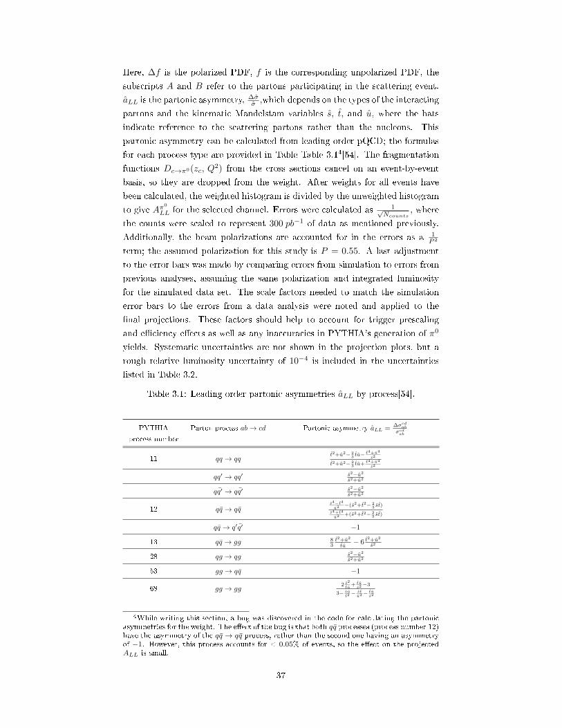
Here, ∆f is the polarized PDF, f is the corresponding unpolarized PDF, the
subscripts A and B refer to the partons participating in the scattering event.
aLL is the partonic asymmetry,∆σσ ,which depends on the types of the interacting
partons and the kinematic Mandelstam variables s, t, and u, where the hats
indicate reference to the scattering partons rather than the nucleons. This
partonic asymmetry can be calculated from leading order pQCD; the formulas
for each process type are provided in Table Table 3.14[54]. The fragmentation
functions Dc→π0(zc, Q2) from the cross sections cancel on an event-by-event
basis, so they are dropped from the weight. After weights for all events have
been calculated, the weighted histogram is divided by the unweighted histogram
to give Aπ0
LL for the selected channel. Errors were calculated as 1√Ncounts
, where
the counts were scaled to represent 300 pb−1 of data as mentioned previously.
Additionally, the beam polarizations are accounted for in the errors as a 1P 2
term; the assumed polarization for this study is P = 0.55. A last adjustment
to the error bars was made by comparing errors from simulation to errors from
previous analyses, assuming the same polarization and integrated luminosity
for the simulated data set. The scale factors needed to match the simulation
error bars to the errors from a data analysis were noted and applied to the
�nal projections. These factors should help to account for trigger prescaling
and e�ciency e�ects as well as any inaccuracies in PYTHIA's generation of π0
yields. Systematic uncertainties are not shown in the projection plots, but a
rough relative luminosity uncertainty of 10−4 is included in the uncertainties
listed in Table 3.2.
Table 3.1: Leading order partonic asymmetries aLL by process[54].
PYTHIA
process number
Parton process ab→ cd Partonic asymmetry aLL =∆σcd
ab
σcdab
11 qq → qqt2+u2− 2
3 tu−t4+u4
s2
t2+u2− 23 tu+ t4+u4
s2
qq′ → qq′ s2−u2
s2+u2
qq′ → qq′ s2−u2
s2+u2
12 qq → qqs4−t4
u2 −(s2+t2− 23 st)
s4+t4
u2 +(s2+t2− 23 st)
qq → q′q′ −1
13 qq → gg 83t2+u2
tu− 6 t
2+u2
s2
28 qg → qg s2−u2
s2+u2
53 gg → qq −1
68 gg → gg2 s2
tu+ tu
s2−3
3− sut2− st
u2− tus2
4While writing this section, a bug was discovered in the code for calculating the partonicasymmetries for the weight. The e�ect of the bug is that both qq processes (process number 12)have the asymmetry of the qq → qq process, rather than the second one having an asymmetryof −1. However, this process accounts for < 0.05% of events, so the e�ect on the projectedALL is small.
37

3.2.1 PDF Sets Used for Aπ0
LL Projections
In generating the weights for the asymmetries (Equation 3.3), for the unpolar-
ized PDFs fA,B we use �ts from a QCD global analysis by the CTEQ (Coor-
dinated Theoretical-Experimental Project on QCD) collaboration [55]. For the
polarized PDFs ∆fA,B , we use results from de Florian, Sassot, Stratmann, and
Vogelsang (DSSV)[22]. Presently, the unpolarized PDFs and the total u− and d-
quark polarized distributions are well-known, whereas the polarized sea-quark
PDFs are less well-constrained, and the polarized gluon PDF is weakly con-
strained, particularly at high and low x (see Figure 1.7). To examine the e�ect
of di�erent models of ∆g(x) on Aπ0
LL, we also generate projected asymmetries
for models of ∆g(x) that di�er from DSSV's best �t.
3.2.2 Modi�ed ∆g(x) Functions
Because we are interested in possible divergences from the DSSV �t to ∆g(x,Q2)
for low x where there is a lack of data, we constructed hypothetical low-x tails
to examine the e�ect on Aπ0
LL. The ∆g's we use, in addition to the standard
�t DSSV-STD and its upper and lower uncertainty limits DSSV-MAX, and
DSSV-MIN, were of the form
∆g(x,Q2 = 10GeV 2) =
k ×DSSV-MAX x < 0.05
DSSV-STD x > 0.05. (3.4)
The constants k were chosen to give values of ∆G[10−3,1.0] ranging from -.7 to
.7. Similarly, we generated ALL projections for ∆g(x) = k × DSSV-MAX over
the whole range of x. The Q2 evolution of the gluon PDF was assumed to be
independent of the scale factor k and was taken from grids provided by DSSV.
Figure 3.4: ∆g(x) from standardDSSV �t, as well as DSSV MIN andMAX from ∆χ2 = +/ − 2%. Allfunctions are scaled by x.
Figure 3.5: DSSV-MAX ∆g(x)compared to g(x)(red) andxg(x)(blue). All functions arescaled by a factor of x.
38

3.2.3 ALL Simulation Results
Projected asymmetries were generated for each of 19 handmade ∆g's overall.
A sample of results from these projections is shown in Figure 3.6 and . The
values of < Aπ0
LL > listed in the table are from �tting the plots of ALL vs. pT
to a constant, and a common factor of 10−4 is dropped from all numbers for
readability. In the Single π0 MPC channel, the �rst point is excluded from the
�t because the dominance of statistics in the lowest pT bin resulted in the �t
reporting the value of Aπ0
LL at that point as the constant. Of particular relevance
for our physics analysis is the small size of the projected asymmetries, even for
models of gluon polarization on the upper end of the range consistent with
experimental data to this point. The simulations point to asymmetries smaller
than 10−3 which would be too small to be seen with the levels of systematic
uncertainty present in ALL measurements at PHENIX in 2009. This concern
motivates our work to limit our systematic uncertainty from our measurement
of the relative luminosity to on the order of 10−4, as we will discuss in depth in
chapter 4.
Even from this limited sample of data, it is possible to identify trends that
point to the low-x region's being probed. First, as a sanity check, it is clear
that the magnitude of the asymmetry increases for all channels as the chosen
∆G[10−3,1.0] increases, and the asymmetry appears to be sensitive to the sign of
∆G. However, when comparing the increase in Aπ0
LL as ∆G[10−3,1.0] is ratcheted
up, the change is much more dramatic for the �forward� channels involving the
MPC than for the �central� channels. The modi�cation of ∆g(x) to bring about
the increase in the truncated moment all occurs at low x. Since the central
channels access less of this range, they are less a�ected by the modi�cation.
However, the forward measurements that do probe the low-x region are very
sensitive to di�erences in the form of ∆g(x) in that region. Of the two forward
channels, the single π0 channel is more sensitive to ∆G because of the higher
statistics available. More concretely, the single π0 MPC measurement could
measure a total gluon polarization of 0.35 at around a 2σ di�erence from zero.
For a ∆G[10−3,1.0] equal to .7 (for the unscaled DSSV-MAX), the di�erence
from zero increases to 5σ. The asymmetries for the di-hadron channel are indeed
larger, indicating a narrower focus on the lower x region of the gluon distribution.
Unfortunately, unlike for the single pion measurement, statistical uncertainties
factor in even more heavily than projected systematic uncertainties.
39

Table 3.2
Table 3.2: Sample of projected Aπ0
LL's �t to a constant, uncertainties, and# of sigmas from 0 with a common factor of 10−4 omitted. The error∆Aπ
0
LL =√
(∆AstatLL )2 + (∆AsysLL )2, using projected AsysLL = 10−4. �CA� refersto the central arm.
∆g(x) =→ DSSV-STD DSSV-MAXDSSV-MAX at low
x
∝DSSV-MAX
∆G[10−3,1.0] =
−0.35
∝DSSV-MAX
∆G[10−3,1.0] = 0.1
Single π0 CA −.1± 1.0(.1σ) 3.8± 1.0(4σ) 2.9± 1(2.9σ) −0.4± 1(−0.39σ) 0.22± 1(0.22σ)
Double π0 CA 1.9± 5.8(.3σ) 2.7± 5.8(.5σ) 2.2± 4.4(0.5σ)−0.75±
4.4(−0.17σ)0.032±4.4(0.0073σ)
π0 MPC+π0 CA −.026± 6.4(.004σ) 6.4± 6.4(1σ) 4.8± 6.6(0.73σ) −1.8± 6.6(−0.28σ) 0.64± 6.6(0.098σ)
Single π0 MPC −.32± 1.2(.3σ) 6.5± 1.0(5σ) 6.4± 1.4(4.7σ) −3.7± 1.4(−2.7σ) 0.75± 1.4(0.56σ)
Double π0 MPC −.34± 14.(.02σ) 12.± 14.(.9σ) 9.8± 6.2(1.6σ) −6.5± 6.2(−1σ) 0.81± 6.2(0.13σ)
π0 MPC N+π0 MPC S −.24± 10.(.02σ) 7.6± 10.(.7σ) 6.5± 4.8(1.4σ) −2.9± 4.8(−0.6σ) 0.63± 4.8(0.13σ)
Figure 3.6: Sample ALL Projections for di�erent channels and ∆g's; only sta-tistical errors shown (does not include projected systematic error of ∼ 10−4).
Single π0 in the CA, DSSV-STD Single π0 in the MPC,
DSSV-STD
Two π0's in the MPC,
DSSV-STD
Single π0 in the CA,
DSSV-MAX
Single π0 in the MPC,
DSSV-MAX
Single π0 in the MPC,
∆g(x < 0.05) =DSSV-MAX,
∆g(x > 0.05) =DSSV-STD
3.3 E�ect of multi-parton interactions and
initial- and �nal-state radiation in PYTHIA
Some of the results from PYTHIA di�er from what would be expected from a
leading order treatment of calculations of kinematics of the involved processes.
This leads to some features of the distributions of x1 and x2 that may not
40

be physical. The main discrepancy is in the range of x accessed by the cen-
tral arm. Previous studies in PHENIX have shown that for p + p collisions at√s = 500GeV , the lower limit of x probed by the central arm is about 5×10⁻³
for 2.0 GeV/c < pT < 2.5 GeV/c, with < x >∼a few times 10−2. The distri-
butions in this note on the other hand show the central arm probing x below
10−3. Furthermore, the x1 range for single π0's in the MPC shows a broad
second hump in addition to the high x quark peak that resembles the x2 dis-
tribution. This symmetrical portion of the distributions is not fully understood
for the forward-boosted collisions that result in π0's in the MPC. Finally, upon
closer examination of kinematic variables on an event-by-event basis, we see a
signi�cant number of events where x2 � x1, indicating a large boost in the
direction of the south MPC, but π0's still show up in the north MPC, or vice
versa. This collection of evidence points toward a weakened connection between
the kinematics of the hard scattering event and the π0's in the �nal state.
Two tunable features of events in PYTHIA can possibly explain these dis-
crepancies: Multi-Parton Interactions (MPIs) and initial- and �nal-state radi-
ation (ISR+FSR). In an event with MPIs, there can be multiple binary in-
teractions between partons in the colliding protons in addition to the hardest
scattering event that is reported by PYTHIA. These can yield additional π0's
that pass our kinematic cuts and are weighted and counted in the same way
as π0's from the primary interaction. For example, consider an event with two
scattering processes: a primary collision (a) and a secondary collision (b). For
the primary collision, we take xa1 � xa2 . This type of collision should result in a
forward boost and π0a's in the forward direction. In the secondary collision, we
can instead have xb1 � xb2, with π0b 's detected in the opposite arm of the MPC.
However, because PYTHIA only reports xa1 and xa2 for each event, the π0b 's will
be mistakenly treated as if they also originated in the primary collision. As a
result, we can see π0's in the opposite arm of the MPC than would be expected
from kinematic considerations based on the reported x1 and x2.
ISR and FSR also can confuse the issue of the proper x1 and x2 to use as the
arguments to the parton distribution functions. When the partons involved in
the hard scattering process radiate gluons, their momentum fractions change.
Additionally, it is possible that the radiated gluons themselves enter the hard
scattering process. Finally, because the radiation processes can themselves be
hard, it is possible that gluons radiated in the initial or the �nal state fragment
directly into π0's that pass the kinematic cuts. It is possible that given our
leading-order calculation of Aπ0
LL and the partonic asymmetries for the projec-
tions, we should not include MPIs, ISR, or FSR from PYTHIA. As a low-level
illustration of the e�ects of MPIs, ISR, and FSR, we include two x distributions
for single π0's for a smaller set of PYTHIA events with MPIs, ISR, and FSR
switched o�.
41

Figure 3.7: x distributions for singleπ0's in the central arm with MPIs,ISR, and FSR switched o�
Figure 3.8: x distributions for singleπ0's in the MPC with MPIs, ISR,and FSR switched o�
42

Chapter 4
Relative Luminosity Analysis
4.1 Overview
One of the main challenges faced in calculating ALL = 1PbPy
N++−RN+−
N+++RN+− to high
precision is determining R, the ratio of the luminosity in same-sign helicity
collisions versus opposite-sign helicity collisions. Particularly in view of the
150 pb−1 of integrated luminosity recorded in Run 13 (compared to the 16.7 pb−1
in Run 11), we hope to push the uncertainty on relative luminosity down to the
order of 10−4. This note is a continuation of work done towards improving the
precision of our relative luminosity measurement over the years in PHENIX,
most recently by groups at Stony Brook University and the University of Illinois
at Urbana-Champaign[56, 57, 58]. In this note, however, we are working chie�y
with scalers with no vertex cut1, as this has been enabled by the STAR scalers
which allow a wider variety of scaler data to be collected. For a summary of the
scalers used in this section, see subsection 2.2.4.
As has been the practice in PHENIX, we use the BBC to determine relative
luminosity due to its good z-vertex resolution and high rates. Nevertheless, we
must be careful not to blindly trust the yields measured by the BBC as rep-
resentative of the true collision rate. In order to maximize our con�dence in
the collision rates as measured by the BBC, we eliminate runs or crossings with
abnormalities in the scaler data through an extensive quality assurance analysis
(section 4.2). Additionally, the limitation that the BBC can only count one
coincidence in a crossing necessitates a rate-dependent correction that accounts
for crossings with multiple collisions (section 4.3). Finally, we limit the possibil-
ity of the BBC itself measuring an ALL through comparison with the luminosity
measured in the second luminosity monitor in PHENIX, the ZDC (section 4.4).
It is the size of the asymmetry ALL(ZDCwideBBCwide ) and its pattern dependence that
serve as our primary estimators of δR.
This chapter ends with a discussion on the crossing dependence of the pileup
corrected ZDCwideBBCwide ratio that is the main driver of poor
√χ2/NDF values in
bunch-�tting ALL(ZDCwideBBCwide ) calculations (section 4.6).
1The ZDCwide trigger actually has a cut at |z| = 150 cm, corresponding to the location ofthe BBC to avoid the ZDC sampling collisions where the BBC has no acceptance. In practice,
this does not make much di�erence, as the average ofZDC(no vtx. cut)
ZDCwideis 1.5× 10⁻⁵.
43

4.2 Scaler data quality assurance
In PHENIX, we have a number of cross-checks on the �goodness� of the scalers
that record the number of triggers from the BBC and ZDC on a run-by-run,
crossing-by-crossing basis. The triggers are recorded by the GL1 scalers, which
sum scalers over all crossings, and the GL1p and STAR scalers, which count
triggers from each of the 120 bunch crossings over the course of a run. We
look for consistency in the data as reported by the three systems and exclude
runs or crossings where discrepancies indicate glitches in the DAQ. Abnormal
data from the scalers, such as a large number of counts in the abort gaps where
no collisions occur, can point to problems with the beam during certain runs.
The shift crews responsible for collecting data during Run 11 also report in
logbooks when they encounter problems during a run that could lead to suspect
data. These considerations all factor into whether a particular run or crossing
is included in the �nal analysis as detailed below.
4.2.1 Run-level QA cuts
Missing STAR scaler data In 29 of the 432 runs designated as �Physics�
runs, there is no STAR scaler data available, making the runs unusable for our
analysis.
STAR scaler bunch structure problems The abort gaps and the four
�empty-full� crossings where only either the blue beam or yellow beam is �lled
are identi�able as crossings where the STAR scalers show greatly reduced counts
in the BBC and the ZDC. In some cases, the gap is �misaligned,� not comprised
of crossings 111-119, but the alignment can be �xed by hand. In other cases,
the abort gap seems to be missing altogether, indicating a malfunction in the
scalers. These problematic runs are excluded from the analysis.
STAR scaler ZDC bunch structure problems We exclude a handful
of runs where the normal bunch structure is present in the BBC scalers, but
problems in the ZDC electronics lead to the abort gaps not appearing in the
ZDC scalers.
STAR-GL1 scaler mismatch The GL1 boards, which integrate trigger
counts over all 120 bunch crossings, provide another cross-check on the accuracy
of the readings from the STAR scalers. The STAR scalers have a slightly delayed
start time at the beginning of each run, resulting in distributions of STARscalersGL1 scalers
that peak between 0.99 and 1.0. We require that this fraction for the clock
triggers, BBCwide triggers, BBCnarrow triggers, and ZDCwide triggers, falls
between 0.99 and 1.0 for all runs included in the analysis.
44

Figure 4.1: Distribution of ratios of STAR scalers to GL1 scalers from each run.
STAR-GL1p scaler mismatch The STAR scalers can also be compared
to the GL1p scalers on a crossing-by-crossing level. Individual crossings where
the ratio of the two scalers falls outside of a range from 0.998 to 1.004 are con-
sidered bad, and these are excluded (see below in the bunch-level QA section).
However, runs with more than six of these bad crossings are removed entirely
from the analysis.
Empty crossing issues In each run, crossings 38, 39, 78, 79, and 111-119
are expected to have few collisions recorded by the STAR scalers due to either
or both of the beams having no proton bunch at that crossing. In a number of
runs, there are either additional �empty� crossings before or after the expected
ones, or some of the crossings expected to be empty register numbers of collisions
consistent with the interaction of two bunches. It is not known whether these
runs exhibit a problem in the timing of the electronics or if there are actual
irregularities in the bunch structure in RHIC, but we exclude these runs in any
case.
Early runs We exclude the period in Run 11 before run 336000, which is
characterized by somewhat unstable beam performance in RHIC, as evidenced
by a low fraction of runs declared suitable for physics analysis, high backgrounds,
and large variations in the ratio of single-arm to coincidence counts in the ZDC
and the ratio of ZDC coincidences to BBC coincidences.
45

4.2.2 Bunch-level QA
Figure 4.2: Database information for individual bunches from one run. Thenumber of π0s reconstructed from MPC analysis is also included. The STARscaler histograms are scaled to appear together on the plot, and the beam spininformation is a constant if a reported helicity is present in the spin databaseand zero otherwise.
In addition to excluding entire runs from the �nal analyzed data set, we drop
individual crossings on a run-by-run basis based on criteria listed below.
Spin information QA The blue and yellow bunches in each crossing are
�lled with either positive or negative helicity, and this information is recorded
in a database. Bunches that are either un�lled or missing their helicity identi�-
cation are excluded from the analysis. In general, these are crossings 38, 39, 78,
and 79, which are the so-called �empty-full� crossings where only either the blue
or yellow beam is �lled, and crossings 111 through 119, the abort gap, which
are never �lled in either beam.
STAR scaler outliers For each run, we plot the value of each of the
six STAR scalers we use versus bunch crossing. We �t these to a constant
using an algorithm that ignores outliers to get the run average. Then, any
crossing i for which scaleri < 0.5 × (scaler average for run) or scaleri > 2 ×(scaler average for run) is excluded.
STAR-GL1p mismatch In comparing the STAR scalers to the GL1p
scalers, we �nd that the ratio for the majority of crossings in all good runs
falls between 0.998 and 1.004. Crossings where this is not the case in any of
46

the scalers present in both the STAR scalers and the GL1p (i.e. BBC30cm,
BBCnarrow, ZDCwide, and ZDCnarrow) are excluded.
Figure 4.3: Trigger live times from the STAR scalers.
Livetime issues/crossing analysis QA In Run 11, there were large
variations in livetime, the ratio of triggers when the DAQ was live (ready to write
data) to total triggers, over the course of the 120 crossings (see Figure 4.3) . In
particular, there is a large drop around crossing 20 and a �recovery� after crossing
82. The presence of the abort gap from crossings 111-119 and the empty-full
crossings also a�ect the livetime of the early crossings. We �nd that because the
e�ect of livetime on the ZDC and BBC is di�erent, including crossings around
these points can have unusual e�ects on the calculated asymmetries between
the BBC and the ZDC. For this reason, we exclude crossings 0, 21, 40, 80, 81,
and 82.
4.2.3 Scaler data QA Summary
The �nal relative luminosity analysis encompasses data from 23,305 good cross-
ings in 239 good runs. The results of the QA are shown in Figure 4.4. The good
runs are listed in Appendix A.
47
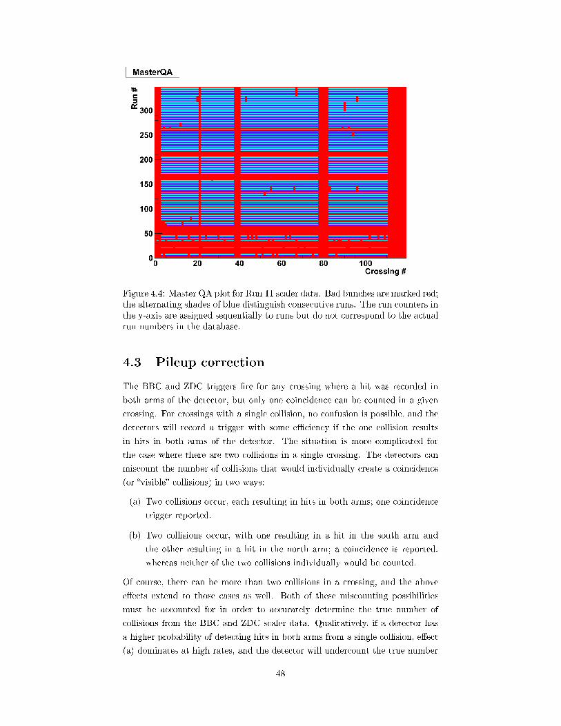
Figure 4.4: Master QA plot for Run 11 scaler data. Bad bunches are marked red;the alternating shades of blue distinguish consecutive runs. The run counters inthe y-axis are assigned sequentially to runs but do not correspond to the actualrun numbers in the database.
4.3 Pileup correction
The BBC and ZDC triggers �re for any crossing where a hit was recorded in
both arms of the detector, but only one coincidence can be counted in a given
crossing. For crossings with a single collision, no confusion is possible, and the
detectors will record a trigger with some e�ciency if the one collision results
in hits in both arms of the detector. The situation is more complicated for
the case where there are two collisions in a single crossing. The detectors can
miscount the number of collisions that would individually create a coincidence
(or �visible� collisions) in two ways:
(a) Two collisions occur, each resulting in hits in both arms; one coincidence
trigger reported.
(b) Two collisions occur, with one resulting in a hit in the south arm and
the other resulting in a hit in the north arm; a coincidence is reported,
whereas neither of the two collisions individually would be counted.
Of course, there can be more than two collisions in a crossing, and the above
e�ects extend to those cases as well. Both of these miscounting possibilities
must be accounted for in order to accurately determine the true number of
collisions from the BBC and ZDC scaler data. Qualitatively, if a detector has
a higher probability of detecting hits in both arms from a single collision, e�ect
(a) dominates at high rates, and the detector will undercount the true number
48

of collisions. If the detector instead has a higher probability of detecting a hit
from a collision in only one arm, the dominant e�ect from multiple collisions
is the accidental coincidences of e�ect (b), and the detector will overcount the
true number of visible collisions.
4.3.1 Derivation of the pileup correction
We now turn to the question of formalizing the pileup correction, following a
derivation by members of the ATLAS collaboration.[59]. We start with a true
rate µ = Ncollisions
Nclock, representing the average number of inelastic pp collisions
per bunch crossing. We assume that the number of collisions in a crossing
obeys Poisson statistics, such that, for the rate µ, the probability of n collisions
occurring in a crossing is
P (n; µ) =µne−µ
n!. (4.1)
We also de�ne e�ciency for a given detector to �see� a hit from a collision in
the south arm, the north arm, or both arms as εS , εN , and εNS respectively;
this e�ciency by de�nition incorporates the detector's acceptance. The true
rates of hits in the detector then are µS = µεS , µN = µεN , and µNS = µεNS .
By extension, we also have εOR = εS + εN − εNS as the e�ciency of at least
one arm of the detector seeing a hit from a collision2. Finally, we have actual
observed single-arm and coincidence rates, NS
Nclock, NN
Nclock, and NNS
Nclock. With these
assumptions and de�nitions, we can begin to work out the relation between true
and observed rates.
Our goal is to determine the value of µvis = µεNS from the scaler values NS ,
NN , NNS , and Nclock. We have that the probability of detecting a coincidence
in a detector (PAND) is one minus the probability of detecting zero hits in at
least one arm (we will call this P0, OR), or
PAND = 1− P0, OR = 1− (P0,S + P0,N − P0,N && 0,S), (4.2)
where the �nal term is the probability that neither arm sees a hit. The proba-
bility for each term on the right-hand side can be determined from the Poisson
distribution:
NNSNclock
= 1− ((µεS)0e−µεS
0!+
(µεN )0e−µεN
0!− (µεOR)0e−µεOR
0!)
= 1− e−µεS − e−µεN + e−µ(εS+εN−εNS). (4.3)
2This follows from the relation P (Aor B) = P (A) + P (B)− P (A&&B).
49

Finally, we introduce the single-arm to double-arm hit ratios3,
kN(S) =εN(S)
εNS. (4.4)
Substituting these ratios into Equation 4.3, the relation simpli�es:4
NNSNclock
= 1− e−µεNSkS − e−µεNSkN + e−µεNS(kS+kN−1)
= 1− e−µNSkS − e−µNSkN + e−µNS(kS+kN−1). (4.5)
This equation cannot be solved for the true rate µNS analytically, but given the
measured rate NNS
Nclockand kN and kS , we can �nd µNS numerically.
4.3.2 Determination of singles-to-doubles ratios for the
ZDC and the BBC
The singles-to-doubles ratios can be found from the single-arm and coincidence
scalers available in the STAR scalers. However, these scalers also depend on
rate due to pileup, so we attempt to correct for this before calculating kN and
kS . We already have the framework above to derive the relation between the
single-arm scaler counts and the true rate of collisions visible to a single arm of
the detector:NS(N)
Nclock= 1− P0,S(N) = 1− e−µεS(N)
µεS(N) = µS(N) = −ln(1−NS(N)
Nclock). (4.6)
If we plug Equation 4.6 into Equation 4.3, we have the following:
NNSNclock
= 1− eln(1− NSNclock
) − eln(1− NNNclock
)+ e
ln(1− NSNclock
)eln(1− NN
Nclock)eµεNS ,
which after simplifying the exponentials and taking the logarithm gives us an
equation for the rate-corrected coincidence rate in terms of only the observed
scalers:
µNS = ln(1− NSNclock
− NNNclock
+NNSNclock
)− ln(1− NSNclock
)− ln(1− NNNclock
). (4.7)
These pileup-corrected values for the singles and doubles rates are what we
use to calculate kN and kS , but why can we not just jump straight to using
Equation 4.7 for our pileup-corrected rates instead of using Equation 4.5? There
are two di�culties with the �scalers-only� approach to the pileup corrections.
3In PHENIX, this value is often de�ned as the ratio of exclusive single-arm counts to the
double-arm counts such that k′N(S)
=εN(S)−εNS
εNS= kN(S)−1 in terms of the de�nitions used
in this section.4Using the exclusive singles-to-doubles ratio, kN(S) → 1 + k′
N(S), so NNS
Nclock= 1 −
e−µNS(1+ks) − e−µNS(1+kN ) + e−µNS(1+kS+kN ).
50
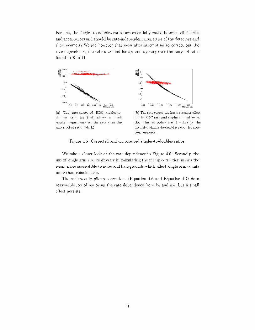
For one, the singles-to-doubles ratios are essentially ratios between e�ciencies
and acceptances and should be rate-independent properties of the detectors and
their geometry.We see however that even after attempting to correct out the
rate dependence, the values we �nd for kN and kS vary over the range of rates
found in Run 11.
(a) The rate-corrected BBC singles-to-
doubles ratio kS (red) shows a much
smaller dependence on the rate than the
uncorrected ratio (black).
(b) The rate correction has a stronger e�ect
on the ZDC rate and singles-to-doubles ra-
tio. The red points are (1 − kS) (or the
exclusive singles-to-doubles ratio) for plot-
ting purposes.
Figure 4.5: Corrected and uncorrected singles-to-doubles ratios.
We take a closer look at the rate dependence in Figure 4.6. Secondly, the
use of single-arm scalers directly in calculating the pileup correction makes the
result more susceptible to noise and backgrounds which a�ect single-arm counts
more than coincidences.
The scalers-only pileup corrections (Equation 4.6 and Equation 4.7) do a
reasonable job of removing the rate dependence from kS and kN , but a small
e�ect persists.
51
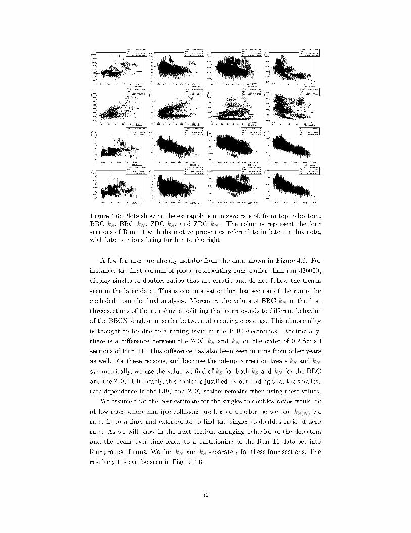
Figure 4.6: Plots showing the extrapolation to zero rate of, from top to bottom,BBC kS , BBC kN , ZDC kS , and ZDC kN . The columns represent the foursections of Run 11 with distinctive properties referred to in later in this note,with later sections being further to the right.
A few features are already notable from the data shown in Figure 4.6. For
instance, the �rst column of plots, representing runs earlier than run 336000,
display singles-to-doubles ratios that are erratic and do not follow the trends
seen in the later data. This is one motivation for that section of the run to be
excluded from the �nal analysis. Moreover, the values of BBC kN in the �rst
three sections of the run show a splitting that corresponds to di�erent behavior
of the BBCN single-arm scaler between alternating crossings. This abnormality
is thought to be due to a timing issue in the BBC electronics. Additionally,
there is a di�erence between the ZDC kS and kN on the order of 0.2 for all
sections of Run 11. This di�erence has also been seen in runs from other years
as well. For these reasons, and because the pileup correction treats kS and kN
symmetrically, we use the value we �nd of kS for both kS and kN for the BBC
and the ZDC. Ultimately, this choice is justi�ed by our �nding that the smallest
rate dependence in the BBC and ZDC scalers remains when using these values.
We assume that the best estimate for the singles-to-doubles ratios would be
at low rates where multiple collisions are less of a factor, so we plot kS(N) vs.
rate, �t to a line, and extrapolate to �nd the singles-to-doubles ratio at zero
rate. As we will show in the next section, changing behavior of the detectors
and the beam over time leads to a partitioning of the Run 11 data set into
four groups of runs. We �nd kN and kS separately for these four sections. The
resulting �ts can be seen in Figure 4.6.
52

Run range BBC kS BBC kN ZDC kS ZDC kN
331130-336000 0.2292 0.2309 3.597 3.381
336000-338000 0.2258 0.2330 3.694 3.436
338000-339700 0.2292 0.2241 3.665 3.495
339700-340515 0.2389 0.2585 3.772 3.616
Table 4.1: Summary of results of singles-to-doubles ratio determination
In practice, there is still enough variation in kN and kS within each section
to justify an attempt to determine the ratios on even shorter timescales. We
�nd that the statistics and lever arm in the ZDCwide rates on the level of an
individual run are not quite su�cient to give stable �ts and values of kN and kS .
However, if we consider each �ll individually, we �nd values that agree well with
the �section-level� values while giving us increased sensitivity to �uctuations in
the singles-to-doubles ratios. For these reasons, for each �ll, we use one value
of BBC kS for BBC kS and kN for all crossings, and likewise for the ZDC.
For the uncertainties on kN and kS , we use the approximate spread on the
values at a given rate over a section of the run. We conservatively estimate that
δ(BBC kS) = ±0.005 and δ(ZDC kS) = ±0.05.
(a) Rate dependence of BBC k′S = kS − 1
for a single �ll. Each point represents one
crossing from the �ll, and the colors repre-
sent runs in the �ll. The rate dependence
within a single run is not strong enough to
extrapolate from, but a clear correlation is
seen over the entire �ll.
(b) The same plot as 4.7a without run
numbers, but error bars and a linear �t
have been added to show the extrapolation
to the zero-rate value of BBC kS = 0.2279.
Figure 4.7: Determination of BBC kS for a single �ll.
53

(a) Rate dependence of ZDC k′S = kS − 1
for a single �ll. Each point represents one
crossing from the �ll, and the colors repre-
sent runs in the �ll. The rate dependence
within a single run is not strong enough to
extrapolate from, but a clear correlation is
seen over the entire �ll.
(b) The same plot as 4.8a without run
numbers, but error bars and a linear �t
have been added to show the extrapolation
to the zero-rate value of ZDC k′S = 3.703.
Figure 4.8: Determination of ZDC kS for a single �ll.
4.3.3 E�ect of the pileup correction
As mentioned before, detectors that see a large singles-to-doubles ratio are likely
to overcount collisions due to accidental coincidences from multiple collisions in
a single crossing hitting a single arm of the detector, whereas detectors with a
small singles-to-doubles ratio undercount collisions because multiple collisions
resulting in true coincidences in a single crossing will only be recorded as a single
coincidence. We see this dichotomy clearly in the pileup corrections to the raw
BBCwide and ZDCwide trigger counts. For our calculated values of kS and kN ,
the BBCwide counts need to be multiplied by a factor greater than one that
grows as the rate increases. Conversely, the ZDCwide counts are multiplied by
a factor smaller than one that decreases with increasing rate.
(a) (b)
Figure 4.9: Pileup correction factors for the BBC (a) and ZDC (b).
The necessity of the pileup correction is clearly demonstrated via a ratio
between the scalers from the two detectors, ZDCwideBBCwide . Ideally, the two detec-
tors count coincidences at a rate directly proportional to the true luminosity,
so the two scalers would be related by a factor that is constant with respect
54

to rate. With no pileup correction applied, the ratio increases drastically with
rate. Particularly because our estimate for the uncertainty on the relative lumi-
nosity measurement depends on ZDCwideBBCwide asymmetries, the correction is needed
to ensure that the rates we measure in one detector are consistent with the
other and that both are proportional to the true collision rate. As shown in
Figure 4.10, the pileup corrections successfully eliminate the rate dependence of
the ZDCwideBBCwide ratio.
Figure 4.10: The e�ect of the pileup correction applied to the BBC and theZDC on the ratio ZDCwide
BBCwide is shown. Each point represents one crossing fromone run, and all crossings from Run 11 that pass the data QA in Run 11 areincluded.
To wrap up the discussion from the previous section on the determination
of the singles-to-doubles ratios, we include a comparison of the ZDCwideBBCwide ra-
tios for one section of the run using the scalers-only pileup correction and the
kS , kN pileup correction, showing the improvement resulting from using the
latter method.
55

(a) Rate-dependence of ZDCwideBBCwide
using
the scalers-only pileup correction (Equa-
tion 4.7).
(b) Rate-dependence of ZDCwideBBCwide
using
the pileup correction with kN and kS
(Equation 4.5). No clear rate-dependence
remains over a wide range of rates.
Figure 4.11: Comparison of pileup correction methods.
After the pileup corrections have been applied to the BBCwide and ZDCwide
scalers, we can take a wide look at the scaler ratios from every crossing over
the entirety of Run 11. We �nd the data arranges into four well-de�ned groups
based on run number. Of the four groups, the �rst is not used in the analysis,
the middle two show reasonably consistent values of ZDCwideBBCwide over a wide range
of BBCwide rates, and the last group is usable despite di�culties with the
bunch storage system that arose leading to wide bunches and a larger range ofZDCwideBBCwide .
Figure 4.12: The pileup corrected ZDCwideBBCwide ratios when plotted against rate fall
in di�erent regions depending on run number.
56

4.4 Constraining ALL in the BBC with the ZDC
Even if we assume that the BBC and the scalers are all working perfectly, and
we are able to correctly account for the possibility of multiple collisions in a
single crossing, we could still run into di�culties if a true physics asymmetry is
measured in the BBC. Such an asymmetry would lead to the BBC measuring
di�erent numbers of collisions in same-sign and opposite-sign crossings for the
same beam, and the measured relative luminosity would not be the proper
normalization for the MPC asymmetry.
For example, if the same physical and positive ALL exists for the pT sampled
by the BBC and the MPC, then both detectors will count higher yields for same-
sign collisions than opposite sign collisions, such that N++ = (1 + δ)N+− for
both detectors. With this assumption, we recall the formula we use to calculate
ALL,
AMPC clus.LL (BBC lumi) =
1
|PbPy|
N++MPC −
N++BBC
N+−BBC
N+−MPC
N++MPC −
N++BBC
N+−BBC
N+−MPC
, (4.8)
and it is clear that no asymmetry will be measured despite our assumption that
ALL exists and is positive.
We employ the other luminosity monitor in PHENIX, the ZDC, as assurance
that the BBC is not measuring an ALL that cancels with an asymmetry in the
MPC. While the MPC and BBC both sample hard collisions between protons,
the ZDC samples double-di�ractive interactions, and the chances are remote
that the same ALL would be generated by two completely di�erent physics
processes. We calculate an asymmetry in the ZDC with the respect to the BBC
in an analogous manner as we do for the MPC:
AZDC.LL (BBC lumi) =1
PbPy
N++ZDC −
N++BBC
N+−BBC
N+−ZDC
N++ZDC −
N++BBC
N+−BBC
N+−ZDC
, (4.9)
δAZDCLL (BBC lumi) =1
PbPy
2N++
BBC
N+−BBC
N++ZDCN
+−ZDC
(N++ZDC +N+−
ZDC)2×√
(δN++
ZDC
N++ZDC
)2 + (δN+−
ZDC
N+−ZDC
)2 + (δN++
BBC
N++BBC
)2 + (δN+−
ZDC
N+−BBC
)2. (4.10)
We calculate the δN from the raw scaler counts in each crossing i as binomial
errors on the rate ri = Ni
Nclocks,i:
δNiNclocks,i
=
√ri(1− ri)Nclocks,i
, (4.11)
taking the error on the number of clock triggers as negligible compared to the
57
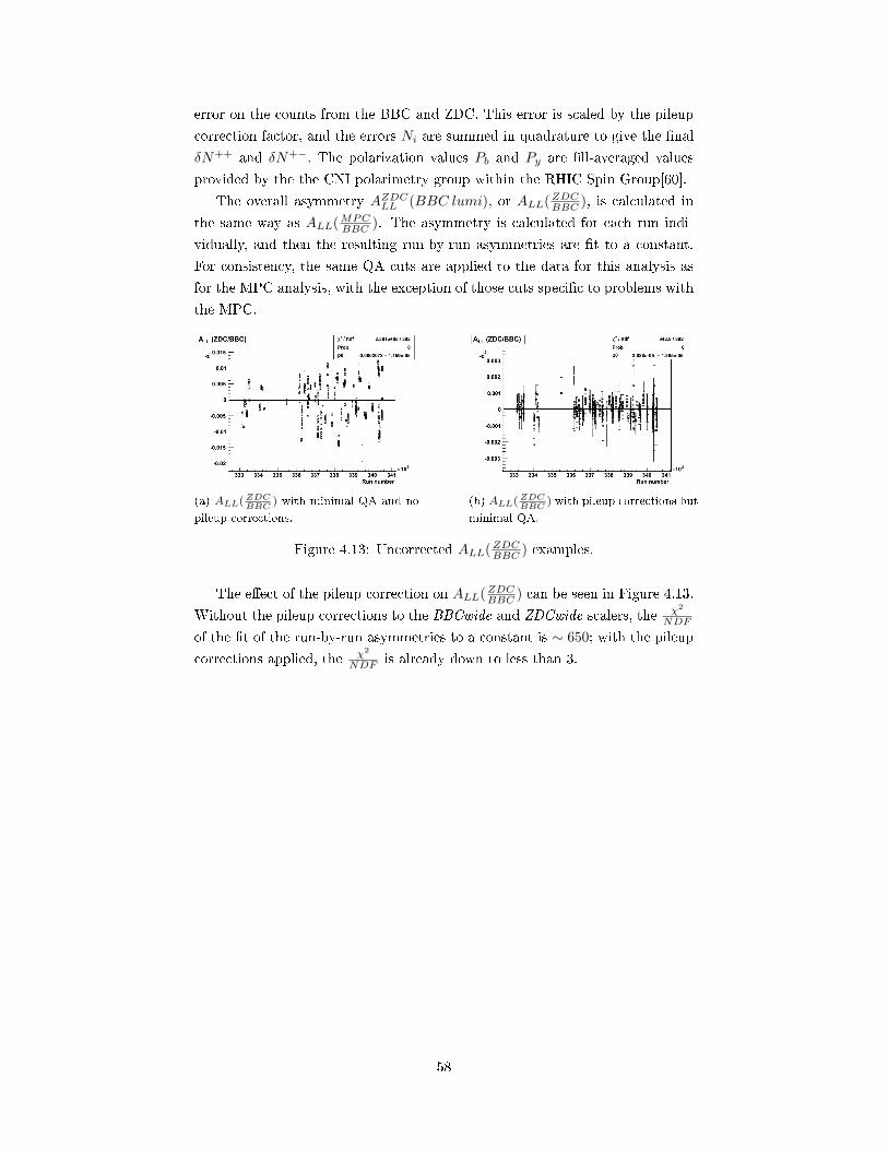
error on the counts from the BBC and ZDC. This error is scaled by the pileup
correction factor, and the errors Ni are summed in quadrature to give the �nal
δN++ and δN+−. The polarization values Pb and Py are �ll-averaged values
provided by the the CNI polarimetry group within the RHIC Spin Group[60].
The overall asymmetry AZDCLL (BBC lumi), or ALL(ZDCBBC ), is calculated in
the same way as ALL(MPCBBC ). The asymmetry is calculated for each run indi-
vidually, and then the resulting run-by-run asymmetries are �t to a constant.
For consistency, the same QA cuts are applied to the data for this analysis as
for the MPC analysis, with the exception of those cuts speci�c to problems with
the MPC.
(a) ALL(ZDCBBC
) with minimal QA and no
pileup corrections.
(b) ALL(ZDCBBC
) with pileup corrections but
minimal QA.
Figure 4.13: Uncorrected ALL(ZDCBBC ) examples.
The e�ect of the pileup correction on ALL(ZDCBBC ) can be seen in Figure 4.13.
Without the pileup corrections to the BBCwide and ZDCwide scalers, the χ2
NDF
of the �t of the run-by-run asymmetries to a constant is ∼ 650; with the pileup
corrections applied, the χ2
NDF is already down to less than 3.
58

Figure 4.14: Final ALL(ZDCBBC ) after the pileup correction and data QA havebeen applied.
With the full data quality assurance cuts applied, problematic crossings and
runs have been removed, bringing the χ2
NDF to 1 and the value of ALL(ZDCBBC ) =
7.298 × 10⁻⁶ ± 1.837 × 10⁻⁵. Generally, the central value of ALL(ZDCBBC ) has
been quoted as δR, the uncertainty on the relative luminosity. As our result is
consistent with zero and smaller than the error on our �t, we instead quote the
error on the �t, 1.837× 10⁻⁵, as the statistical component of δR.
4.5 Checks on systematic errors
As additional veri�cation of the data, our quality assurance methods, and our
calculations, we carry out a number of analyses as cross checks. First, we check
for consistency in ALL(ZDCBBC ) between the four spin patterns used at RHIC dur-
ing Run 11 to ensure that the beam is not a�ected by the particular sequence of
same-sign and opposite-sign crossings. We also compare the asymmetry in even
crossings versus odd crossings to check for e�ects resulting from the separate
trigger circuits in some PHENIX systems that handle alternating crossings. A
third test involving the double spin asymmetry is a bunch shu�ing analysis
wherein asymmetries are calculated with randomized spin patterns to con�rm
that the statistical error we report accurately re�ects the spread of asymmetries
that would be seen if we could repeat our measurement a large number of times.
The last systematic e�ect we attempt to account for involves the pileup correc-
tion; by scanning through a range of values of the singles-to-doubles ratios that
are inputs to the pileup correction, we see how uncertainty in our determination
of those values propagates to an uncertainty in the �nal asymmetry.
59
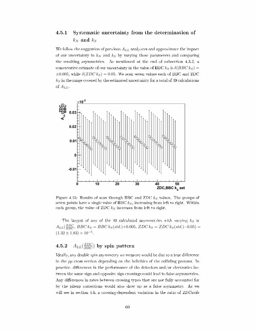
4.5.1 Systematic uncertainty from the determination of
kN and kS
We follow the suggestion of previous ALL analyzers and approximate the impact
of our uncertainty in kN and kS by varying these parameters and comparing
the resulting asymmetries. As mentioned at the end of subsection 4.3.2, a
conservative estimate of our uncertainty in the value of BBC kS is δ(BBC kS) =
±0.005, while δ(ZDC kS) = 0.05. We scan seven values each of BBC and ZDC
kS in the range covered by the estimated uncertainty for a total of 49 calculations
of ALL.
Figure 4.15: Results of scan through BBC and ZDC kS values. The groups ofseven points have a single value of BBC kS , increasing from left to right. Withineach group, the value of ZDC kS increases from left to right.
The largest of any of the 49 calculated asymmetries with varying kS is
ALL(ZDCBBC , BBC kS = BBC kS(std.)+0.005, ZDC kS = ZDC kS(std.)−0.05) =
(1.32± 1.83)× 10−5.
4.5.2 ALL(ZDCBBC
) by spin pattern
Ideally, any double spin asymmetry we measure would be due to a true di�erence
in the pp cross section depending on the helicities of the colliding protons. In
practice, di�erences in the performance of the detectors and/or electronics be-
tween the same-sign and opposite-sign crossings could lead to false asymmetries.
Any di�erences in rates between crossing types that are not fully accounted for
by the pileup corrections would also show up as a false asymmetry. As we
will see in section 4.6, a crossing-dependent variation in the ratio of ZDCwide
60

to BBCwide scalers can lead to an asymmetry that is independent of physics
considerations.
The false asymmetries cause maximal splitting between the two �SOOS�
patterns and the two �OSSO� patterns (de�ned by the pattern of same-sign and
opposite-sign blue and yellow beam helicities in the �rst four crossings) shown
in Table 4.2.
Table 4.2: Spin pattern de�nitions for Run 11
Spin Pattern Crossings 0-7
P0 (SOOS)Blue beam helicity
Yellow beam helicity
+−+−−+−+
+ +−−+ +−−
P1 (SOOS)Blue beam helicity
Yellow beam helicity
−+−+ +−+−−−+ +−−++
P2 (OSSO)Blue beam helicity
Yellow beam helicity
+−+−−+−+
−−+ +−−++
P3 (OSSO)Blue beam helicity
Yellow beam helicity
−+−+ +−+−+ +−−+ +−−
For example, consider a hypothetical distribution of scalers (BBC and ZDC)
that are functions of the crossing numbers only: NBBC(ZDC)(crossing). We
then choose a spin pattern such that the scalers are summed according to their
crossing types, and we plug these totals into Equation 4.9:
PbPyASOOSLL (
ZDC
BBC) =
N++ZDC −
N++BBC
N+−BBC
N+−ZDC
N++ZDC +
N++BBC
N+−BBC
N+−ZDC
.
If we instead use the other type of spin pattern (switching from SOOS to OSSO),
the result is that the identi�cation of each crossing type switches such that in
Equation 4.9, N++ → N+−. Making this substitution back into the formula for
the asymmetry, we obtain the same result, but with a minus sign:
PbPyAOSSOLL (
ZDC
BBC) =
N+−ZDC −
N+−BBC
N++BBC
N++ZDC
N+−ZDC +
N+−BBC
N++BBC
N++ZDC
=
N++BBC
N+−BBC
N+−ZDC −N
++ZDC
N++BBC
N+−BBC
N+−ZDC +N++
ZDC
(4.12)
= −PbPyASOOSLL (ZDC
BBC).
Therefore, we take di�erences in ALL(ZDCBBC ) to be indicative of a false asym-
metry that depends on the details of our particular measurement in PHENIX
rather than a physics asymmetry. We place limits on the size of this type of false
asymmetry by calculating the asymmetry separately for the four spin patterns.
We demonstrate in Figure 4.16 that the asymmetries from all four patterns are
61

consistent with zero and with one another (within 1σ).
Figure 4.16: Double spin asymmetries are shown calculated separately for �llsin Pattern 0 (black, SOOS-type), Pattern 1 (red, SOOS-type), Pattern 2 (blue,OSSO-type), and Pattern 3 (violet, OSSO-type). The asymmetries from thefour patterns are consistent with zero and with one another, and the �ts havereasonable values of χ2/NDF .
4.5.3 Parity-violating single-spin asymmetries
We also construct the longitudinal single spin asymmetries between the ZDC
and the BBC for the blue (yellow) beam,
AL,b(y)(ZDC
BBC) =
1
Pb(y)
N+ZDC −
N+BBC
N−BBC
N−ZDC
N+ZDC +
N+BBC
N−BBC
N+ZDC
,
where the N+is the sum of all scalers in crossings where the blue (yellow) beam
has helicity of +1, while N− is the sum for crossings where the beam has helicity
−1.
A non-zero asymmetry would violate parity conservation, which is impossible
for the strong force. In fact, as can be seen in Figure 4.17, a large asymmetry
is seen in both beams. The cause of this asymmetry is unknown at present, but
the interplay between beam angles or o�sets and a physical AN in the beam
resulting from residual transverse polarization seems to be a good candidate,
as proposed by Andrew Manion and Kieran Boyle[61]. It appears that the
single spin asymmetry in the scalers does not negatively impact our double spin
asymmetry measurements though; any problem would show up as a non-zero
double spin asymmetry in the scalers, which we do not see.
62

(a) AL(ZDCBBC
) for the blue beam. (b) AL(ZDCBBC
) for the yellow beam.
Figure 4.17: AL(ZDCBBC ) results showing a non-zero parity-violating asymmetry.
4.5.4 Bunch shu�ing
The bunch shu�ing test has previously been carried out on �nal physics asym-
metries (e.g. Aπ0
LL) as a check for systematic errors and the accurate deter-
mination of statistical errors. For completeness, I perform the test here on
ALL(ZDCBBC ). For each run, we randomly assign the blue and yellow helicities for
each crossing. With these randomized spin patterns, we recalculate ALL(ZDCBBC ).
As the bunch shu�ing eliminates any relationship between the assigned helici-
ties of a crossing and the true helicities, the e�ective polarization of the shu�ed
data is zero, meaning we expect asymmetries that are consistent with zero within
the statistical uncertainties. The shu�ing procedure is repeated 10,000 times
for each run to get a distribution of asymmetries. We �nd the total asymmetry
for each of the 10,000 shu�es from a �t to the asymmetry vs. run number
(as in the physics case), and we generate a histogram �lled with the value ofALL
δALL(stat.) for each shu�e. We expect the resulting distribution to be centered
at zero to re�ect the unpolarized nature of the shu�ed data, and the width of
the distribution should be near one if the statistical errors on ALL(ZDCBBC ) are
accurately determined.
63

(a) ALL(ZDCBBC
) bunch shu�ing distribu-
tion. Each entry is ALLδALL
for the entire
Run 11 data set (with QA cuts). For this
distribution, σ = 4, in contrast to the ex-
pectation that σ = 1.
(b) Bunch shu�ing widths for individual
runs. No runs are excluded from this plot
by run QA, though runs with extremely
large widths are not shown due to the y-
axis scale.
Figure 4.18: ALL(ZDCBBC ) bunch shu�ing results.
However, it is clear from Figure 4.18 that the bunch shu�ing test fails badly
for the scaler asymmetries. The same behavior is seen in the bunch shu�ing
of the single-spin asymmetries as well. It appears that the statistical errors
signi�cantly underrepresent actual �uctuations in the data. In contrast to our
�ndings from the bunch shu�ing procedure, in our �nal result for ALL(ZDCBBC )
in Figure 4.14, the χ2
NDF is essentially 1, indicating that the statistical errors
used are appropriate. Ultimately, we �nd that the large shu�ing widths are
caused by variations of the ratio of ZDC to BBC scalers over the 120 crossings
in a run. This variation is signi�cant compared to the statistical error, but
normal spin patterns employed at RHIC were designed to limit the impact on
asymmetries of such crossing-dependent �uctuations. Bunch shu�ing leads to
unphysical distributions of same-sign and opposite-sign crossings that cause a
crossing dependence of ZDCwideBBCwide to become problematic. We investigate this
concept further in section 4.6.
4.5.5 Even-odd separated ALL(ZDCBBC
)
The di�erence in BBC kN between even-numbered and odd-numbered crossings
motivates the calculation of ALL(ZDCwideBBCwide ) for even and odd crossings sepa-
rately.
64

Figure 4.19: ALL(ZDCBBC ) for even and odd crossings separately.
(a) ALL(ZDCBBC
) for even crossings only. (b) ALL(ZDCBBC
) for odd crossings only.
The χ2/NDF of the �ts as well as the size of the asymmetries are a bit worse
than for the combined even and odd crossings. This is likely an artifact of the
same e�ect causing the wide shu�ing widths, namely the crossing dependence
of the ZDCwideBBCwide ratio. As mentioned in the previous subsection, this e�ect
is mitigated by the close and even distribution of same-sign and opposite-sign
crossings that ensures that both types of crossings sample similar ZDCwideBBCwide ratios
over the course of the 120 crossings. The spacing between crossing types is
increased when only considering every second crossing in a run. We demonstrate
in Figure 4.20 the continued deterioration of the asymmetry �ts for increased
crossing spacing by considering asymmetries comprised from data only from
every third crossing, every fourth crossing, and so on.
65

Figure 4.20: ALL(ZDCwideBBCwide ) for every nth crossing, for n = 3 to n = 7. Forn = 8, the crossings included in the analysis would all be either same-sign oropposite-sign due to the periodicity of the spin pattern, so no asymmetry canbe calculated.
4.6 Variation in ZDCwideBBCwide with crossing number
We found in the course of the relative luminosity analysis that while on a large
scale (e.g. the sections of Run 11 used for determining kN and kS), the pileup
corrections are e�ective and su�cient for ensuring consistent luminosity mea-
surements between the ZDC and the BBC, this is not the case on the level of
an individual run (see Figure 4.21). The problem is evident when consider-
ing a method of determining the run-by-run asymmetry via the bunch �tting
method5. In this method, we de�ne a function relating the ZDCwideBBCwide at each
crossing nC to the blue and yellow beam helicities for that crossing and a �raw�
5The bunch �tting method is mathematically equivalent to calculating ALL by summingscalers in same-sign and opposite-sign crossings as is done in this chapter. The �tting methodgives more information (via the χ2/NDF ) about how �well-behaved� the data is on a crossing-to-crossing level.
66

asymmetry:
(ZDCwide
BBCwide)nC
= α(1 + Sy,nCSb,nC
εLL), (4.13)
where Sb(y),nC= +1 if the blue (yellow) bunch at crossing nC has positive helic-
ity and−1 if it has negative helicity, and εLL = PbPyALL(ZDCwideBBCwide ). Attempting
to �t data with large non-statistical �uctuations in ZDCwideBBCwide with Equation 4.13
yields very large values of χ2/NDF that call into question the validity of the
�t.
Figure 4.21: The scaler ratios from run 339134 show the characteristic relationto crossing number, peaking around crossing twenty and consistently falling o�during the remaining crossings. The �t parameters show the result of the bunch�tting method for this run (Equation 4.13).
We can clarify the impact of the variation in ZDCwideBBCwide on our asymmetry
calculations by rewriting Equation 4.9 with neither the ZDC nor BBC distin-
guished as the �yield� detector or the �relative luminosity� detector:
AZDC.LL (BBC lumi) =1
|PbPy|
N++ZDC
N++BBC
− N+−ZDC
N+−BBC
N++ZDC
N++BBC
− N+−ZDC
N+−BBC
. (4.14)
We see here that ALL(ZDCBBC ) compares the pileup corrected ZDCwideBBCwide ratios
in same-sign crossings to the ratios in opposite-sign crossings. We would expect
this di�erence to be negligible in the absence of a physical asymmetry in particle
production between the same-sign and opposite-sign crossings. However, we see
from the average values of ZDCwideBBCwide as a function of crossing number that an
opposite-sign crossing could have a smaller ZDCwideBBCwide than a same-sign crossing
simply by having a larger crossing number.
67

Fortunately, we will see in the �nal calculation of ALL(ZDCBBC ) that this prob-
lem is not fatal. The spin patterns employed at RHIC ensure an even distri-
bution of ++ and +- crossings, such that the average crossing number of the
crossing types are near one another. Roughly speaking, we have that the ratiosZDCwideBBCwide are modi�ed by a crossing-dependent factor:
ZDCwide
BBCwide→ ZDCwide
BBCwide× f(crossing#). (4.15)
If we assume that ZDCwideBBCwide has no double spin asymmetry, then the ALL we
measure is only sensitive to di�erences in the values of f between ++ and +-
crossings. Abbreviating the crossing number as nC , we have
ALL(ZDC
BBC) ∼< f(nC) >++ crossings − < f(nC) >+− crossings . (4.16)
Finally, as f(nC) is more or less linear, we estimate that < f(nC) >= f(< nC >
), so we write
ALL(ZDC
BBC) ∝ f(< nC >++ crossings)− f(< nC >+− crossings),
which goes to zero as the di�erence in average crossing number between same-
sign and opposite-sign crossings goes to zero.
While we escape trouble with the crossing-dependent ZDCwideBBCwide ratio when
considering the overall ALL(ZDCBBC ), the pattern is problematic in other ways.
First, a method for determining ALL(ZDCBBC ) on a run-by-run basis using a
method known as bunch �tting yields �ts with very large values of χ2
NDF (see the
�t parameters in Figure 4.22, for example), complicating the identi�cation of
the bunch-by-bunch statistical errors with true statistical �uctuations. A second
point, related to the �rst, is that the bunch shu�ing check on systematic errors
breaks down. Finally, from a philosophical standpoint, if our goal is to pre-
cisely understand the relationship between the BBC's measurement of relative
luminosity and the true relative luminosity and to con�rm our understanding
with the ZDC, we would like to understand why the two detectors count di�er-
ently with respect to one another as a function of crossing number. We discuss
attempts to address these issues in a future section. In the meantime, we will
show how the ZDCwideBBCwide variations lead to large bunch shu�ing widths and why
this e�ect is not a concern for the �nal analysis.
4.6.1 E�ect of crossing-dependent ZDCwideBBCwide
variation on
bunch shu�ing widths
We return to Equation 4.14 and consider how bunch shu�ed asymmetries are
a�ected by a systematic variation in the ratio ZDCwideBBCwide that depends on crossing
number. As explained in the previous section, such a variation is not problem-
atic as long as same-sign and opposite-sign crossings are �evenly distributed�
68

over crossing numbers as they are in the data. However, bunch shu�ing creates
helicity con�gurations where same-sign crossings (or more accurately, crossings
that have been randomly assigned a same-sign con�guration) are more con-
centrated at early or late crossings compared to opposite-sign crossings. The
strong correlation between crossing number and ZDCwideBBCwide means that for earlier
crossings, ZDCwideBBCwide is larger than in later crossings. Therefore, when calcu-
lating ALL(ZDCBBC ), a shu�e with more same-sign crossings at early crossings
will tend to have larger values that enter into the positive term of the numer-
ator of Equation 4.14, while the opposite-sign crossings at later crossings have
smaller ZDCwideBBCwide values entering into the negative term in the numerator. The
resulting ALL,shuf.(ZDCwideBBCwide ) will be positive by virtue of whatever e�ect causes
ZDCwideBBCwide to vary with crossing number, independent of a di�erence between the
cross sections of same-sign and opposite-sign crossings. This e�ect is stronger
for runs with larger slopes in the relation between ZDCwideBBCwide versus crossing num-
ber, while the e�ect is mitigated somewhat in runs with less statistics, where
the increased uncertainty on ZDCwideBBCwide from crossing to crossing can mask the
crossing dependence to some degree.
Figure 4.22: ZDCwideBBCwide vs. crossing for one run; disparity in the locations of
same-sign and opposite-sign crossings can lead to false asymmetries.
We can demonstrate that the unexpectedly large bunch shu�ed asymme-
tries arise from unphysical helicity con�gurations by de�ning a scaler-weighted
average crossing number for same-sign and opposite-sign crossings:
< SS crossings >=
∑SS crossings nC ×BBCwide∑
SS crossingsBBCwide,
69
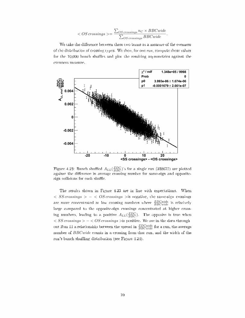
< OS crossings >=
∑OS crossings nC ×BBCwide∑
OS crossingsBBCwide.
We take the di�erence between these two terms as a measure of the evenness
of the distribution of crossing types. We then, for one run, compute these values
for the 10,000 bunch shu�es and plot the resulting asymmetries against the
evenness measure.
Figure 4.23: Bunch shu�ed ALL(ZDCBBC )'s for a single run (338677) are plottedagainst the di�erence in average crossing number for same-sign and opposite-sign collisions for each shu�e.
The results shown in Figure 4.23 are in line with expectations. When
< SS crossings > − < OS crossings >is negative, the same-sign crossings
are more concentrated at low crossing numbers where ZDCwideBBCwide is relatively
large compared to the opposite-sign crossings concentrated at higher cross-
ing numbers, leading to a positive ALL(ZDCBBC ). The opposite is true when
< SS crossings > − < OS crossings >is positive. We see in the data through-
out Run 11 a relationship between the spread in ZDCwideBBCwide for a run, the average
number of BBCwide counts in a crossing from that run, and the width of the
run's bunch shu�ing distribution (see Figure 4.24).
70

Figure 4.24: The e�ect of ZDCwideBBCwide variation and statistical precision on bunchshu�ing widths in the data is shown in this 2D histogram. For small averageBBCwide counts, the statistical error bars cover the variation in ZDCwide
BBCwide (asmeasured by the slope vs. crossing) to some extent, reducing the e�ect on thebunch shu�ing widths. The measurement of ZDCwideBBCwide for each crossing becomesmore precise with increasing BBCwide counts, at which point the e�ect ofincreasing slopes of ZDCwideBBCwide on bunch shu�ing widths becomes apparent.
While the widths of the bunch shu�ing distributions are adversely a�ected
by the crossing dependence of ZDCwideBBCwide , we show through our determination of
ALL(ZDCBBC ) that the problem has a negligible impact on our �nal uncertainty on
relative luminosity. In Figure 4.25, we plot ALL(ZDCBBC ) vs. < SS crossings >
− < OS crossings >instead of run number, �t to a constant in 4.25a and a
line in 4.25b .
71

(a) ALL(ZDCBBC
) vs. < SS crossings >
− < OS crossings > �t to a constant.
(b) ALL(ZDCBBC
) vs. < SS crossings > − <OS crossings > �t to a line; this �t only
o�ers a minuscule improvement in χ2
NDF
compared to the constant �t. There is
a slight dependence of ALL(ZDCBBC
) on the
helicity con�guration, but only at a level
slightly above 1σ.
Figure 4.25: Dependence of ALL(ZDCBBC ) on distribution of same-sign andopposite-sign crossings.
We further con�rm our hypothesis that the increased bunch shu�ing widths
come from the form of ZDCwideBBCwide vs. crossing number by generating test cases
of data for hypothetical runs. The typical spread in ZDCwideBBCwide over a run is
(ZDCwideBBCwide )max−(ZDCwideBBCwide )min = 0.001. We use spreads of 0, 0.0004, 0.001, and
0.003 in the test data. As mentioned before, the total number of scaler counts
in a run also determines how statistically signi�cant a given spread of scaler
ratio values is, so we tune this number as well. We choose a typical value of
BBCwide to generate one test data set, and two other sets are generated with13 and 3 times the typical value of BBCwide.
(a) A test run of data generated with the
assumption that ZDCwideBBCwide
does not de-
pend on crossing number. The scalers in
each crossing are randomly shifted accord-
ing to a Gaussian error distribution.
(b) A test run of data generated with a
large variation in ZDCwideBBCwide
and a large
number of statistics. Both are about 3x
what is seen in a typical run of real data.
Figure 4.26: Examples of ZDCwideBBCwide vs. crossing from test data.
We bunch shu�e the test data sets in the same manner as for the real
data; the results are shown in Figure 4.27. We see that as the slope of the
correlation between ZDCwideBBCwide and crossing number increases (moving down the
72

rows in Figure 4.27), the bunch shu�ing widths increase from around one to
greater than eight, with increased statistical precision (moving to the right in
Figure 4.27) amplifying the e�ect of the slope on the widths even further.
Figure 4.27: Bunch shu�ing for test data. Each row represents one choice forthe spread in ZDCwide
BBCwide as discussed in the text, with the spread starting at 0in the top row and increasing for the following rows. Each column representsone of the selection for the total BBCwide counts; the �rst column is 1
3 of thetypical value, the middle column is the typical value, and the third column is 3times the typical value.
73

4.6.2 The nature of the ZDCwideBBCwide
dependence on crossing
number
Even if the combination of statistics and the crossing dependence of the scaler
ratio ZDCwideBBCwide in Run 11 is not enough to signi�cantly increase our uncertainty
in determining relative luminosity, this may not be the case in future runs with
higher luminosity, longer runs, and di�erent variations of ZDCwideBBCwide with crossing
number. For this reason, we have undertaken further studies of this systematic
e�ect in hopes of understanding the cause.
4.6.2.1 Form of the dependence
The qualitative features of the graph of ZDCwideBBCwide vs. crossing are very similar
across all runs and all sections of Run 11. The main feature is a linearly de-
creasing trend starting around crossing 20 with notable outliers that tend to fall
around the empty-full crossings. The �rst twenty crossings are less consistent
but tend to have ZDCwideBBCwide scaler ratios that begin at nearly the same level as
some of the later crossings but quickly rise to a peak around crossing 20. To
demonstrate the universality of this e�ect, we plot the scaler ratio and crossing
number for each crossing passing QA cuts from all runs in a section of Run 11.
(a) ZDC-to-BBC ratios from all good
crossings from runs between 338450 and
339700.
(b) For each crossing, the statistics-
weighted average for all crossings in a sec-
tion of Run 11 is plotted against the cross-
ing number.
Figure 4.28: Scaler ratios vs. crossing for runs between 338450 and 339700.
74

Figure 4.29: Scaler ratio splines for the four sections of Run 11.
We can also examine the strength of the correlation between ZDCwideBBCwide and
crossing number for each run. This correlation can be measured either by a
correlation factor or from the slope of a linear �t to ZDCwideBBCwide vs. crossing
number. The correlation factor between the set of ordered pairs (ZDCwideBBCwide , nC)
in a run is given by
corr(ZDCwide
BBCwide, nC) =
cov(ZDCwideBBCwide , nC)
σZDCwideBBCwide
σnC
.
The correlation factor method is disadvantageous in that it does not account
for error bars, while using the slope instead as a measure of correlation can
tell us how big of an e�ect results from the correlation but not how good the
correlation is. For both measures, we exclude the �rst 20 crossings that tend
not to follow the same trend as the remaining crossings, as discussed above.
75

(a) The distribution of correlation fac-
tors between the scaler ratios and crossing
number within individual runs is shown.
Nearly all runs show a signi�cant negative
correlation meaning ZDCwideBBCwide
decreases
with increasing crossing number.
(b) Slopes of linear �ts to the data are all
negative. A slope of −5 × 10⁻⁶ over 90
crossings (from 20 to 110) corresponds to a
decrease in the scaler ratio of 0.00045 or a
change of −0.5% for a typical ZDCwideBBCwide
of
0.083.
Figure 4.30: Strength of correlation between scaler ratio and crossing numberin individual runs.
4.6.2.2 Correlation between the scaler ratio and other variables
We have other information in the data on the level of an individual crossing,
including coincidence rates, singles rates, singles-to-doubles ratios, and measures
of the width of the collision vertex distribution6. By looking at how this other
data varies with crossing number and for correlations between these data and
the scaler ratios, we try to understand the underlying cause of the crossing
dependence of ZDCwideBBCwide . We present here distributions of correlation factors on
the level of individual runs between ZDCwideBBCwide and these data.
(a) Run-by-run correlation factors betweenZDCwideBBCwide
and BBCwide rate.
(b) Run-by-run correlation factors betweenZDCwideBBCwide
and ZDCwide rate.
Figure 4.31: Correlations between scaler ratios and coincidence rates.
6We use wall current monitor data from each crossing to generate unbiased vertex distri-butions. For more details, see [58].
76

(a) Run-by-run correlation factors betweenZDCwideBBCwide
and BBCS exclusive single-arm
rate.
(b) Run-by-run correlation factors betweenZDCwideBBCwide
and ZDCS exclusive single-arm
rate.
Figure 4.32: Correlations between scaler ratios and south arm exclusive singlesrates.
(a) Run-by-run correlation factors betweenZDCwideBBCwide
and the BBCN exclusive single-
arm rate.
(b) Run-by-run correlation factors betweenZDCwideBBCwide
and ZDCN exclusive single-arm
rate.
Figure 4.33: Correlations between scaler ratios and north arm exclusive singlesrates.
(a) Run-by-run correlation factors betweenZDCwideBBCwide
and BBC kS .
(b) Run-by-run correlation factors betweenZDCwideBBCwide
and ZDC kS .
Figure 4.34: Correlations between scaler ratios and singles-to-doubles ratios.
77

Figure 4.35: Run-by-run correlation factors between ZDCwideBBCwide and the widths
of the vertex distributions derived from wall current monitor data.
(a) Run-by-run correlation factors betweenZDCwideBBCwide
and BBC vertex distribution
RMS.
(b) Run-by-run correlation factors betweenZDCwideBBCwide
and ZDC vertex distribution
RMS.
Figure 4.36: Correlations between scaler ratios and width of vertex distributions.
78

Figure 4.37: Correlation factors between ZDC kS and width of vertex distribu-tions derived from wall current monitor data.
4.6.3 Possible sources of variation in scaler ratio vs.
crossing number
From the plots in subsubsection 4.6.2.2, we see that the best candidates for a
strong correlation to the scaler ratio are the singles-to-doubles ratio (especially
ZDC kS) and the width of the collision vertex distribution as taken from wall
current monitor data. On the whole, we do not see evidence for a correlation
between ZDCwideBBCwide and single-arm or coincidence rates, though there may be
some slight correlations due to correlations between the rates and the other
variables.
Variation of singles-to-doubles ratios within single runs We �rst con-
sider the possible correlation between crossing-to-crossing variations and the
singles-to-doubles ratios. For the purpose of this exercise, we will look at run
338925 from �ll 15419. Over the range of crossings in this run, the scaler ratio
drops from 0.0829 around crossing 20 to 0.0823 around crossing 100, so we have
a percent change of 0.7%. In Figure 4.39, we show the variation in the singles-to-
doubles ratios through the run. In order to use our method of extrapolating to
zero rate to �nd kS for the pileup correction, we can only choose a single value of
kS for each �ll, and we ignore the crossing dependence of the singles-to-doubles
ratios in applying the pileup correction. This imprecision could theoretically
lead to a crossing-dependent error in the pileup correction that could cause the
variation in the scaler ratio. The �raw� BBCS singles-to-doubles ratios (not
extrapolated to zero rate) fall in a range from 0.223 to 0.225. Shifting this
79

range to the zero-extrapolated value for the �ll of 0.22937 and taking from the
data BBCwideuncorr. = 0.26, we �nd that the range of BBC kS values could
account for a change in the corrected BBCwide rate of 0.03%. Similarly, the
range in ZDC kS of ∼ 0.03 could lead to a change in the ZDCwide rate of 0.3%.
While this gets factor gets close to the 0.7% di�erence in the scaler ratio from
crossing 20 to crossing 100, the change would be applied in the wrong direction.
The later crossings have larger ZDC kS than the early crossings; as a larger
ZDC kS yields a smaller corrected ZDCwide rate, the e�ect of implementing
the varying ZDC kS would be to further decrease the ZDCwideBBCwide ratio at higher
crossing numbers. For this reason, it seems more plausible that the crossing-
dependent variation of the singles-to-doubles ratio has a cause in common with
the scaler ratio variation rather than being the cause of the variation through
pileup corrections.
Figure 4.38: ZDCwideBBCwide ratios for Run 338625.
80

(a) Run-by-run correlation factors betweenZDCwideBBCwide
and BBC vertex distribution
RMS.
(b) Run-by-run correlation factors betweenZDCwideBBCwide
and ZDC vertex distribution
RMS.
Figure 4.39: BBC and ZDC south arm singles-to-doubles ratios vs. crossing forRun 338925.
Crossing dependence of collision vertex distribution widths Trends
similar to what we see in the plots of ZDCwideBBCwide vs. crossing are also present in
plots of vertex distribution width vs. crossing (see Figure 4.40).
Figure 4.40: Vertex distribution widths for Run 338925
The scaler ratio could be sensitive to the vertex widths due to di�erences
in acceptance between the BBC and the ZDC. Theoretically, the scaler ratio
variation could also be a result o� the limited ZDC resolution in conjunction
with the �ducial vertex cut at 150 cm for the ZDCwide trigger; we eliminated
this second possibility by generating the scaler ratios using a simple ZDC coin-
cidence trigger from the STAR scalers that did not include a vertex cut. There
was no noticeable di�erence in the crossing dependence of the scaler ratios.
As for detector acceptance e�ects, the ZDC is located at |z| = 18m, we
81

assume its acceptance is �at within z = ±150 cm. We know from Vernier scans
in Run 11, though, that the BBC acceptance falls o� compared to the ZDC as
|z| approaches 150 cm[62].
Figure 4.41: Plot of BBC acceptance as a function of |z|. The data shown is(BBCwide&&ZDCwide)
ZDCwide .
We can use the acceptance function, aBBC(z) = p0 + p1z2, taken from the
�t to modify the raw BBCwide scalers by a factor that increases with increasing
vertex distribution width to account for would-be coincidences that are lost
due to the BBC's limited acceptance at large |z|. To determine the correction
factor, we generate a Gaussian g(z, vtxRMS) centered at z = 0 cm with a width
taken from the wall current monitor data and a �at function, aflat(z) with the
same p0 as the acceptance function. The correction factor is the ratio of the
integral of the Gaussian with no acceptance modi�cation to the integral of the
acceptance-modi�ed Gaussian:
facc =
´ 150
−150g(z, vtxRMS)× aflat(z)dz´ 150
−150g(z, vtxRMS)× aBBC(z)dz
. (4.17)
The correction factor is applied to the BBCwide scalers before pileup corrections.
We use a typical BBCwide rate of 0.26 to demonstrate the �nal impact on the
rates, as a correction applied before pileup corrections will lead to a di�erent
pileup correction factor as well.
82

Figure 4.42: E�ect of z-dependent BBC acceptance on �nal BBCwide rates.
In Figure 4.42, we see that over the range of vertex widths seen during
the course of Run 11, the BBC acceptance factor can change by around 1%.
However, the majority of �lls have a spread in vertex distribution widths less
than 2.5 cm with none greater than 4 cm; therefore, a more realistic expectation
of the e�ect of an acceptance correction is on the order of 0.1%, too small to
account for the ZDCwideBBCwide crossing dependence. Additionally, any correlation
between ZDCwideBBCwide and vertex width is washed out when considering crossings
from many �lls simultaneously in most of Run 11. Interestingly, after the 9 MHz
radio frequency system involved in con�ning protons in bunches failed around
run 339700, a strong correlation between the scaler ratio and the vertex width
reappears along with larger vertex widths in general for the rest of the run.
83

Figure 4.43: Relation between scaler ratios and vertex distribution widths, be-fore and after the failure of the 9 MHz RF cavity around run 339700.
4.7 Summary of relative luminosity status
For the beam intensity in Run 11, the pileup corrections work su�ciently well
and the crossing dependence of ZDCwideBBCwide can be safely ignored for the purposes
of determining relative luminosity. Our �nal value of ALL(ZDCwideBBCwide ), as deter-
mined from a �t to run-to-run calculations of the asymmetry, is (0.88± 1.8)×10−5. We see no systematic dependence of the asymmetry on spin pattern. We
also scan over a range of values of kS and kN for the BBC and ZDC to es-
timate the systematic uncertainty that enters through the pileup correction.
The resulting spread in ALL(ZDCwideBBCwide ) over all scanned values of kS and kN
is 1.3 × 10⁻⁵, though the asymmetries calculated from all scanned values are
consistent with one another. We nevertheless use the spread as an estimate of
this systematic uncertainty.
While we seem to have the uncertainty from relative luminosity under control
in Run 11 without needing to adjust error bars to account for poor χ2/NDF
values in the bunch �tting, it remains to be seen whether the approach set forth
in this note will be as successful in Run 13. The increase in bunch-to-bunch
luminosities in Run 13 may result in the crossing dependence of ZDCwideBBCwide being
a critical problem. We have laid out ideas of where to look for the cause of
the scaler ratio variation, but no single factor seems to explain everything. We
may need to �nally track down the source of the variation and correct for it to
achieve similar precision in our relative luminosity measurement for Run 13 and
beyond.
84

Chapter 5
MPC Calibration
To extract useful physics information from the MPC, we need to convert the
�raw� information provided by the detector, essentially in the form of charge
output and timing from the avalanche photodiodes attached to each crystal in
the detector, to information about the energy deposited by particles incident
on the detector. A comprehensive overview of this process is detailed in an
analysis note written for the PHENIX collaboration[63]. In a condensed form,
the conversion from charge to energy can be represented for each individual
tower i by the following equation:
Ei = ADCi ×Gi ×Ri(t), (5.1)
where ADCi (Analog-to-Digital Converter) is the charge measurement out-
put by the detector for tower i, Gi is the gain, or the charge-to-energy conversion
factor for tower i, and Ri(t) is a factor that accounts for variations in crystal and
APD output over time. Each of the terms on the right are the result of a subset
of the MPC calibration. The ADCi values depend on calibration of the MPC's
front-end electronics module (FEM); the Gi are determined from a calibration
process wherein the detector's ADC representations of energy are mapped to
physical values via comparison to physical parameters, namely known energy
spectra and the π0 mass; and the Ri(t) are measured by an LED monitoring
system that tracks the response of the detector to stable pulses of light delivered
to each crystal individually in the MPC.
5.1 FEM Calibration
What appears in Equation 5.1 as ADCi is calculated o�ine as the combination
of multiple measurements. From the discussion in subsection 2.3.3, we have
ADCi = ADCpost −ADCpre − (ADCpost,pedestal −ADCpre,pedestal) (5.2)
for both the low-gain ADC and the high-gain ADC. A conversion factor between
the low-gain and high-gain ADC must be found to ensure that the low-gain and
high-gain ADC give the same results. Also, we must determine the high-gain
over�ow value, above which the high-gain ADC is no longer suitable for use.
85

The pedestals are calibration constants that are measured when the MPC is
operational but no beam is present. In practice, these values have been found
to be stable over the course of the run and subtract to 0 in the above equation
anyway. Therefore, they are ignored in our analysis.
Additionally, we determine when the low-gain ADC over�ows, at which point
the recorded ADC value is unreliable. TDC over�ow values are also found
and used to isolate towers in the MPC that are out of time from the particles
associated with a collision of interest.
5.1.1 High-gain to low-gain conversion factor/high-gain
cuto�
The ampli�ed (high-gain) ADC yields a higher ADC value for a given energy
than does the low-gain ADC. The readings from tower i are related by the
following equation:ADCi,high
Ci= ADCi,low. (5.3)
The ampli�cation factor for the high-gain ADC was set in the hardware to be
around 16, but the actual value varies slightly from tower to tower. In the
software, this ampli�cation factor is divided out so that a single Gi can be
used for each tower to convert from ADC to energy, regardless of whether the
high-gain or low-gain ADC is used.
To �nd the high/low ratio Ci for a given tower, the point at which the high-
gain ADC over�ows must �rst be identi�ed, as this gives the endpoint of the
range where the high-gain ADCs are valid. To this end, we plot a histogram
of the high-gain ADCpost −ADCpre values. The over�ow is characterized by a
large peak at the end of the falling ADC spectrum; any charge that would be
measured as having an ADC value greater than 4095 is dumped into the last
ADC bin. The peak is lower than 4095 and broadened because the ADC we
record includes the subtracted ADCpre value, which does not over�ow and can
vary. We �nd the characteristic peak at high ADCs and work back to lower
ADCs to �nd the minimum of the spectrum in a certain range. The bins to the
right of this minimum have increasing numbers of counts in contradiction to the
expectation of a consistently falling spectrum, so high-gain ADCs in this range
are potentially misleading over�ows and cannot be used.
86

Figure 5.1: A plot of the high-gain ADC spectrum for one tower. The verticalred line is drawn where an algorithm determined the over�ow to be.
Next, we compare the high-gain and low-gain ADC readings for a large
number of hits in a given tower. We plot the low-gain ADC versus the high-
gain ADC for each hit, and we �t a line in a range bounded on the low end by
0 and on the high end by the high-gain over�ow values we found (see 5.2a).
The inverse of the slope of this line gives us the constant Ci from Equation 5.3.
Alternatively, we can generate a one-dimensional histogram of the ratio of the
high-gain to low-gain ADC values for a tower. The peak (taken either as the
mean of the histogram or as the peak of a Gaussian �t to the histogram) would
also give us an estimate of Ci.
87

Figure 5.2: Methods for �nding the low-gain conversion factor.
(a) Here, the low gain ADC is plotted
vs. the high gain ADC, and the ratio is
found from the slope of the line �t to the
graph. The blue line represents the high
gain over�ow point and serves as the up-
per limit for the �t.
(b) The distribution of high gain ADC to
low gain ADC ratios is shown. The con-
version factor can be taken as the mean of
this distribution.
Ultimately, for each tower, we compared the resulting low-gain ADC spec-
trum and the high-gain ADC spectrum scaled by 1Ci, for each of the meth-
ods mentioned above for determining Ci. A �matching factor� M is de�ned:
M =∑# of binsk
1# of bins |Nk(highADCCi
)−Nk(lowADC)|, where the Nk are thenumber of counts N in histogram bin k. Whichever Ci gives the smallest value
of M for tower i is the �nal value used.
88

Figure 5.3: Comparison of the high gain ADC spectrum (black), scaled downby the conversion factor, to the low gain ADC spectrum (red).
5.1.2 ADC, TDC Over�ows
The low gain ADCs and the TDCs for each tower can over�ow in the same way
as the high gain ADC over�ows discussed in the previous section. The low gain
ADC over�ow corresponds to an amount of energy deposited in a crystal (or
more directly, charge collected in the APD) that surpasses the dynamic range
of the ADC. A TDC over�ow for a channel indicates a hit that came too late for
the TDC to receive the stop signal, where the TDC start time is determined by
the BBC's measurement of the collision time. A cut based on the TDC over�ow
helps to eliminate out-of-time particles not originating from the pp collision.
The same procedure is used to �nd the over�ows for the low-gain ADCs, the
high-gain ADCs, and the TDCs. An example plot showing the over�ow determi-
nation for the high-gain ADC was included in the previous section in Figure 5.1;
we present examples for the low-gain ADCs and the TDCs in Figure 5.4.
89
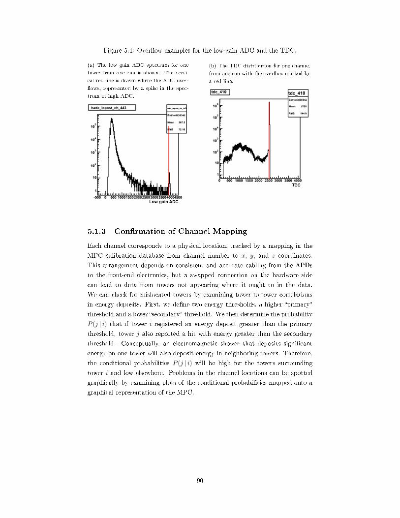
Figure 5.4: Over�ow examples for the low-gain ADC and the TDC.
(a) The low gain ADC spectrum for one
tower from one run is shown. The verti-
cal red line is drawn where the ADC over-
�ows, represented by a spike in the spec-
trum at high ADC.
(b) The TDC distribution for one channel
from one run with the over�ow marked by
a red line.
5.1.3 Con�rmation of Channel Mapping
Each channel corresponds to a physical location, tracked by a mapping in the
MPC calibration database from channel number to x, y, and z coordinates.
This arrangement depends on consistent and accurate cabling from the APDs
to the front-end electronics, but a swapped connection on the hardware side
can lead to data from towers not appearing where it ought to in the data.
We can check for mislocated towers by examining tower-to-tower correlations
in energy deposits. First, we de�ne two energy thresholds, a higher �primary�
threshold and a lower �secondary� threshold. We then determine the probability
P (j | i) that if tower i registered an energy deposit greater than the primary
threshold, tower j also reported a hit with energy greater than the secondary
threshold. Conceptually, an electromagnetic shower that deposits signi�cant
energy on one tower will also deposit energy in neighboring towers. Therefore,
the conditional probabilities P (j | i) will be high for the towers surrounding
tower i and low elsewhere. Problems in the channel locations can be spotted
graphically by examining plots of the conditional probabilities mapped onto a
graphical representation of the MPC.
90

Figure 5.5: Conditional probabilities for a channel with correct location map-ping. The tower in question has by de�nition P (i | i) = 1, but its value is set to0.15 to avoid distorting the color axis. The bright colors surrounding the towerare neighboring towers with comparatively high P (j | i), while the probabilitiesfor towers further away to be hit are vanishingly small.
When scanning through the towers, we found a section of the MPC South
a�ected by an accidental swapping of signal cables that send data from the MPC
to a driver board.
91

Figure 5.6: An error in the cabling for the MPC was uncovered through thechannel mapping analysis. The top row shows a sequence of four adjacenttowers before the mapping was corrected. The �rst two towers from the left arenormal, but the third and fourth plots reveal towers that must be near eachother in physical space but are separated in the data. The bottom row showsthe same towers after the mapping was corrected.
Ultimately, we found that eleven towers were swapped one-to-one with eleven
other towers. The issue was corrected in the reconstruction software by a simple
reassignment of the a�ected channel numbers.
5.1.4 Noise subtraction from problematic driver board
A considerable excess of counts is present in both the low-gain and high-gain
ADC spectra for one of the driver boards in the north arm of the MPC compared
to other channels.
92

Figure 5.7: Location of the noisy driver board in the MPCN (driver board 19).
(a) Low-gain ADC spectrum from one run
for Ch. 416 in the noisy driver board com-
pared to an una�ected channel.
(b) High-gain ADC spectrum from one run
for Ch. 416 in the noisy driver board com-
pared to an una�ected channel.
Figure 5.8: The noisy driver board is evident in both the low-gain and high-gainADC spectra.
We attempt to correct for the noise in the reconstruction code. If > 50%
of the channels in the noisy driver board (at least 10 of the 19) register a hit,
we calculate a truncated mean of the energies recorded by the noisy channels,
excluding the two highest and two lowest energies. This truncated mean energy
is then subtracted from each tower in the driver board, with the goal of removing
the correlated noise in the channels while leaving real energy deposits from a
particle shower intact.
93

5.2 LED Calibration
Analyzers have access to ADC measurements of a �xed amount of light delivered
to the crystals from LEDs via optical �bers twice a second throughout Run 11
(see subsection 2.3.2). The mean ADC recorded from LED pulses for channel
i for a run we write as LEDi(run). We compare these values for each run and
each tower to the values from a reference run to get the relative gain factor,
Ri(t). As we average LED measurements over the period of one run, we write
Ri(run) = (ADCi(run)
ADCi(ref.))−1,
where the inverse represents the concept that as the e�ciency of the detector
falls below what it was at the reference run (meaning ADCi(run)ADCi(ref) < 1), we need
to correct our measurements by a factor greater than one to compensate. There
are occasional runs or towers for which the LED system drops out, so the values
of Ri(run) for those runs or towers are found from interpolating the values
from nearby runs (since Ri(t) is stable over short periods of time) or from
nearby towers (since temperature and radiation aging e�ects should be similar
for towers in close proximity).
In general, radiation damage throughout the running period causes light to
be transmitted less e�ciently in the PbWO4 crystals as time goes on. The end
result is that for the �xed amount of light delivered to the crystals, we measure
smaller ADC values later in the year than early in the year. The towers closer to
the beam pipe (at smaller r in the MPC) experience higher amounts of radiation,
so the LED correction changes more over time for these towers. We present an
example of this behavior in Figure 5.9.
94

Figure 5.9: The average ADC measurement by run normalized to a referencerun for a row of towers in the MPC at varying distances to the beam pipe r.We see that for long time scales, the ADC measurements decrease for each ofthe towers, while the decline is sharper for towers at small r closer to the beampipe. The jump before run 336636 corresponds to a change in the high-voltagesettings of the MPC (see text).
Fluctuations in the LED output as measured by the APDs can also result
from temperature changes in the MPC. Previous studies have found that the
e�ective gain of the APDs decreases by 2% per increase in temperature of one
degree Celsius[41]. A general warming of the detector occurs throughout the run,
which begins in January and ends in April, and temporary sharp �uctuations
in temperature are attributable to the switching on or o� of the electromagnet
in the muon arm ( 5.10a). The brief variations in temperature correspond to
adjustments in the LED correction factor as well ( 5.10b).
(a) Temperature variations in the MPCS
and MPCN during Run 11.
(b) Temperature in the MPCN along with
the ADC response to the LED for one
channel in the MPCN for a section of Run
11.
Figure 5.10: Temperature variations in the MPC.
95

A key feature of the LED data from Run 11 is the jump that occurs be-
tween runs 336610 and 336636. This point in time corresponds to when the
high voltage setting on the MPC APDs was increased from M=10 to M=15 to
compensate for the cumulative degradation of the detector response both during
Run 11 and since the commissioning of the MPC. This change is re�ected by the
increase of the LED readings from ~ 0.7 before the jump to ~ 1.0 afterwards.
We decided to use a single reference run early in the M=15 portion of Run 11,
run 336739, as the M=15 portion is a higher percentage of the run and the LED
system seems to have no problem accounting for the drastic change in the APD
output.
5.3 Gain Calibration
With the FEM calibrated and time-dependent changes in detector response
accounted for, the �nal step is to translate the ADC values to energies by
�nding the gain Gi for each tower. Previously, an initial estimate could be
found using minimum ionizing particles (MIPs) in the MPC. Such particles lose
a nearly �xed amount of energy per length in the MPC, meaning that the total
energy they deposit can be calculated to be 234 MeV. One could �nd the peak
corresponding to the minimum ionizing particles in the ADC spectrum of a
tower, and the Gi would be simply the ratio of 234 MeV to the ADC value at
this peak. The MIP peak was detectable in earlier runs at lower beam energies
where the voltage to the APD was set to M=50. At higher beam energies,
where M=10 or M=15 to increase the range of energies measurable by the ADC
before it over�ows, the MIP peak gets lost in background and electronics noise,
meaning a di�erent approach to approximate the gains was needed. Initially, we
tried an assumption that the gains would be simply related by the ratio of the
M values for the APDs, but this method was not successful. It appears that the
cumulative aging e�ects on the MPC resulted in lower detector response than
would be expected from this simple analysis, necessitating the use of larger
gains.
5.3.1 Spectrum Matching
Knowing the energy spectrum for each tower from a previous run at the same
center-of-mass energy gives another reference point that allows us to bypass a
MIP analysis and �nd a rough estimate of the gain. For each tower, we can gen-
erate a histogram of hit energies from a reference run in Run 91, normalizing the
histogram with the number of events in the sample. We can also generate ADC
histograms for the same tower from Run 11, again normalizing the histogram
with the number of events. Because the MPC is measuring the same physics in
1The MPC was calibrated in earlier runs based on test beam measurements and detec-tor response to minimum ionizing particles which deposit a known amount of energy in thedetector.
96

2011 as it was in 2009, we can determine which gain, when applied to the ADC
spectrum for a tower, reproduces the �true� energy spectrum from Run 9.
We search for the approximate gain by comparing the counts in a range from
4 GeV to 12 GeV2 of the energy histogram to a range in the ADC histogram. For
the energy histogram, the bins to be integrated over begin with the bin centered
at Emin = 4GeV and end at Emax = 12GeV . For the ADC histogram, the low
bin of the range is the bin containing ADCmin = Emin
Gi×Ri(t) = 4GeV
Gi,itr×Ri(t),
where Ri(t) is the relative gain factor taken from the LED measurements and
Gi,itr is the test gain value that we vary from 0 to 2.0 in steps of 0.001. Similarly,
the high bin of the range is the bin containing ADCmax = Emax
Gi× Ri(t) =
12GeVGi,itr
× Ri(t). For each iteration, starting at Gi,itr = 0.001, we �nd R =∑ibin=ADCmaxibin=ADCmin
NADC(ibin)∑ibin=Emaxibin=Emin
NE(ibin), where the NADC and NE refer to the counts in a bin of
the ADC histogram and the energy histogram, respectively. Once we �nd R ≥ 1,
the iterative procedure is stopped, and we take that Gi,itr as the approximate
gain for tower i. The procedure works quite well for well-behaved towers, as can
be seen in Figure 5.11, comparing a reference spectrum for a tower from Run
9 with an energy spectrum in Run 11 generated with the gain found using the
above method.
Figure 5.11: Sample results from spectrum matching method for �nding. Theblack line is the reference energy spectrum from one tower in Run 9, while thered line is the Run 11 spectrum using the gains from the matching method.
For towers in the noisy driver board, we have mixed results. For some
channels, the noise subtraction cleans up the spectra and allows for a successful
2Using this limited range avoids di�culties due to noise at low energy and poor statisticsat high energy.
97

match; for others, the noise subtraction is not su�cient to salvage the channel.
(a) Energy spectrum comparison for Ch.
443 between Run 9 (black) and Run 11
(red,blue). The red spectrum includes the
noise subtraction algorithm while the blue
does not, and improvement can be seen.
(b) Energy spectrum comparison for Ch.
412 between Run 9 (black) and Run 11
(red,blue). The red spectrum includes the
noise subtraction algorithm while the blue
does not. In this case, the noise subtrac-
tion does not correct the shape of the en-
ergy spectrum at low energy.
Figure 5.12: The noisy driver board is evident in both the low-gain and high-gain ADC spectra.
5.3.2 Iterative π0 Calibration
Once we have an approximation of the correct gains for each tower, we �nalize
the gains by generating di-photon invariant mass spectra, identifying the π0
mass peak, and comparing the mass to what we �nd from simulation. When
a π0 decays into two photons, each photon incident on the MPC initiates an
electromagnetic shower which presents as a contiguous �cluster� of towers with
energy deposits in the MPC. For each cluster, we have position and energy in-
formation which allow us to make selection cuts on the clusters entering into the
di-photon mass spectrum and to calculate the invariant mass of the di-photon
pair. To determine the expected reconstructed π0 mass after energy-leakage and
acceptance e�ects are accounted for, we use simulations based on the PYTHIA
event generator as well as GEANT, a software package that emulates the spe-
ci�c geometry, materials, and response of the detector, giving us an idea even
of how the showering and clustering of particles in the detector are expected to
proceed[64]. The reconstructed π0 masses in each tower from the simulations
are given in Figure 5.13 and Figure 5.14. We �nd that the reconstructed masses
are within 10MeV/c2 of the π0 mass of 135MeV/c2, with more accurate recon-
structions away from the edges of the detector where leakage and acceptance
e�ects lead to smaller reconstructed masses.
98

Figure 5.13: Reconstructed π0 masses for each tower from simulation for theMPC South (left) and North (right).
Figure 5.14: Distribution of tower-by-tower π0 mass peaks as determined fromsimulation. The trueπ0 mass is 135MeV/c, but the segmentation of the MPC,acceptance e�ects, and the particular kinematic cuts we use a�ect the locationof the peak of the di-photon invariant mass spectrum.
On the data side, we begin with a set of cuts on single clusters:
• Central tower of cluster not in warn map (�agged as a malfunctioning
tower)
• Eclus > 2GeV
• 12 cm < rclus < 19 cm
• Dispersion < 4.0 cm2(a measure of lateral extent of the shower; the cut
helps to distinguish EM from hadronic showers)
99

• χ2/NDF < 3 (comparison of shower shape to expected energy pro�le)
• No towers in cluster with an ADC over�ow (see subsection 5.1.2)
• TDC from central tower of cluster is not an over�ow (see subsection 5.1.2)
• Dispersion > 0.0005 cm2 (single tower background cut)
• # towers in cluster > 2 (single tower background cut)
• Ecentral tower
Eclus< 0.95 (single tower background cut)
From the set of all clusters that pass the above cuts, we calculate the invariant
mass M2γγ = E2
γγ − p2γγ = 2E1E2(1 − cos(θ)), where θ is the opening angle
between the two clusters and E1and E2 are the energies of the two participating
clusters. The cluster pairs are subject to additional cuts for the iterative π0
calibration:
• 9GeV < Epair < 17GeV (energy window matched to simulation; avoids
noise at low energy and cluster merging at high energy)
• pT,pair > 0.5GeV/c
• cluster separation > 2.6 cm (to avoid overlapping clusters and associated
di�culties)
• α = |E1−E2|E1+E2
< 0.6 (energy asymmetry cut; improves signal to background
ratio)
For each pair that passes all of the above cuts, a histogram for the central
towers of the two participating clusters is incremented at Mγγ , weighted by the
cluster's share of the pair's energy Eclus
E1+E2.
Once the invariant mass spectra for all towers are generated, we �t the
peak near the π0 mass with a Gaussian in a window with a width of 50MeV
around the peak. We get the π0 mass mi for each tower i from the mean of this
Gaussian. We �nd a correction factor to the gain as the ratio of the mass to the
value from simulation, δ = mi
mi,sim, and we adjust the tower gain accordingly.
With the new tower gains, a simpli�ed clustering algorithm is used to recalculate
cluster energies, though to save computation time, we assume the cluster center
positions are unchanged by the reshu�ing of tower energies within the cluster.
The new cluster energies in turn are used to �nd new π0 mass peaks, and we
converge on the �nal gains for all towers through successive iterations of gain
adjustments and comparisons to the simulated mass peaks.
We �nd in the beginning that our estimated gains from the spectrum match-
ing method are an underestimate as shown in Figure 5.15.
100

Figure 5.15: Initial comparison of reconstructed π0 masses in data to simulation,using the gains from spectrum matching to determine tower energies.
During the course of the iterative process, some towers can be seen to have
diverging behavior, often as a result of either far too few or far too many counts.
These towers are added to the warn map (colored in the maps below with
red diagonal lines) as they come up, and they are excluded from contributing
to invariant mass distributions in other towers. With the exception of these
misbehaving towers and the noisy driver board, the iterative procedure results
in π0 masses from nearly all towers that are within 5% of the target value from
simulation. In Figure 5.16, we compare the �nal reconstructed π0 masses to
the value from simulation and plot the results for individual towers as well as a
distribution. In Figure 5.17 and Figure 5.18, we show the �nal invariant mass
distributions for each tower in the MPC South and MPC North. Finally, in
Figure 5.19, we show by what factor the gains from each tower change over the
course of the iterative procedure; the initial estimated gains were on the average
adjusted upwards by ∼ 15%.
101
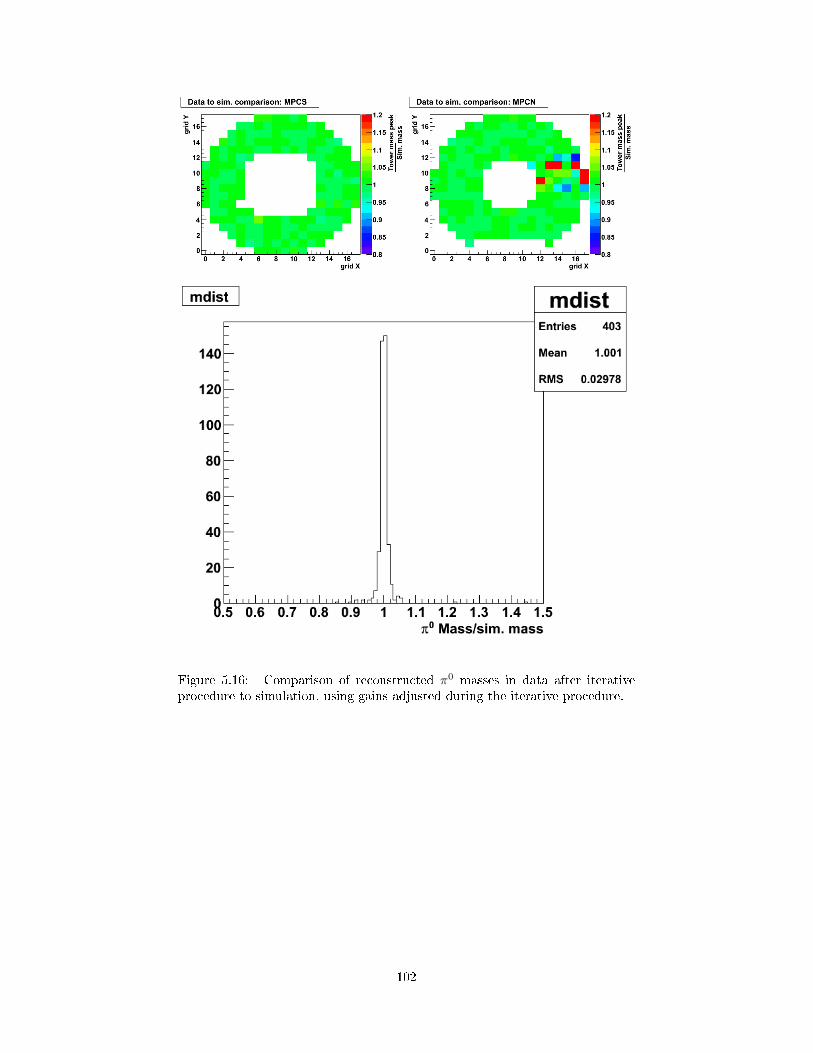
Figure 5.16: Comparison of reconstructed π0 masses in data after iterativeprocedure to simulation, using gains adjusted during the iterative procedure.
102
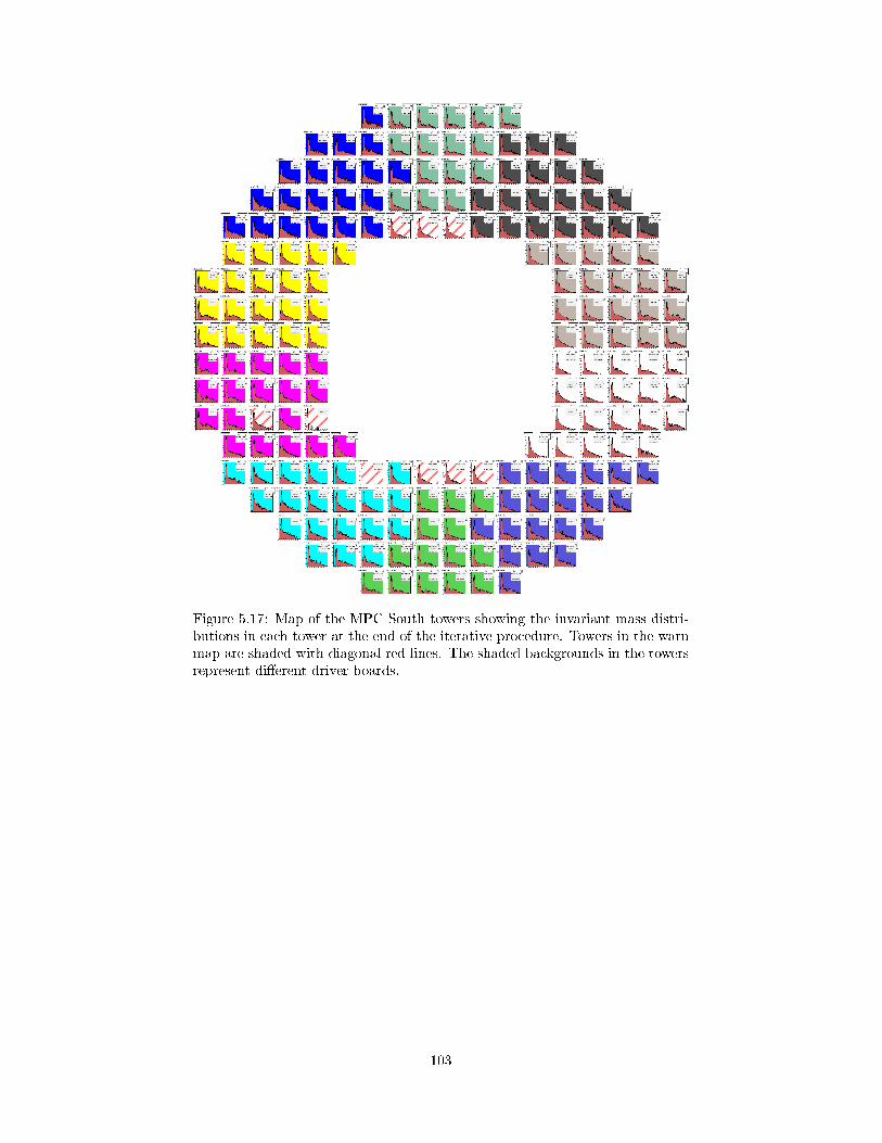
Figure 5.17: Map of the MPC South towers showing the invariant mass distri-butions in each tower at the end of the iterative procedure. Towers in the warnmap are shaded with diagonal red lines. The shaded backgrounds in the towersrepresent di�erent driver boards.
103

Figure 5.18: Map of the MPC North towers showing the invariant mass distri-butions in each tower at the end of the iterative procedure. Towers in the warnmap are shaded with diagonal red lines. The shaded backgrounds in the towersrepresent di�erent driver boards.
104

Figure 5.19: Plots showing the ratio final gaininitial gain for each tower. In the top plot,
the left map represents the MPC South, while the right represents the MPCNorth.
5.4 Warn map analysis
One of the standard cuts used in our �nal analysis is a simple exclusion of
problematic towers in the MPC known as a warn map. The warn map is both
an input and an output to the iterative π0 calibration procedure. The warn
map is needed as input because without a warn map, problematic towers can
skew the invariant mass distributions in other towers and hinder our ability
to accurately determine the correct gains. The warn map however is also an
output from the iterative procedure because we need reasonable gains in order
to determine if towers are �hot� or �cold,� registering too many or too few hits,
respectively, in comparison to other towers in the MPC. For this reason, we
�rst identify towers that are clearly malfunctioning and remove them from the
iterative π0 analysis. Once the iterative π0 calibration is run once, we use the
105

resulting gains to perform a more thorough analysis of hit rates in each tower.
Some care must be taken when comparing the number of hits between dif-
ferent towers. In general, particle production is a function of pseudorapidity η,
and slices in η correspond to rings in the MPC. Rings closer to the center of
the MPC contain fewer towers, so each tower gets a bigger share of the number
of particles, dNdη , for these rings. In other words, while each tower has the same
geometrical size and shape, a tower's span in η and φ depend on r, the distance
from the center of a tower to the center of the beam pipe. In the end, we �nd
that the logarithm of the number of counts per trigger falls roughly linearly
with increasing r. For each run, we �nd the number of counts per minimum
bias trigger in six energy ranges for each tower. We plot log10(cts/trigger) vs.
r and �t with a second degree polynomial (which tracks the relation better at
small and large r), excluding the 15% of towers furthest from the �t to prevent
outliers from dominating the �t. We then �nd the RMS, again excluding the
outliers, and draw bands at ±3σ from the �t as shown in Figure 5.20. Towers
that fall outside of the bands are considered bad for that run and energy bin.
Figure 5.20: Example determination of hot and cold towers in the MPC Southand North for the six energy bins for one run. The �rst two rows are for theMPC South while the last two are for the MPC North. Each individual plotrepresents counts per trigger in a particular energy bin labeled on the plot.
We consider the two sections of Run 11 with di�erent high voltage settings
106

for the MPC separately, and if a tower is bad in more than 10% of runs in a
section for a particular energy range, we say the tower is bad in that range.
Then, if a tower is bad in at least three of the six energy ranges for a section,
we consider it bad for the whole section.
The results for the warn map are shown in Figure 5.21 and Figure 5.22.
The section of the MPCN corresponding to driver board 19 stands out as being
bad as expected. A few of the towers are malfunctioning and were essentially
inoperable during Run 11, while the cause of the other bad towers is less clear.
In some cases, possibly again due to noise, the π0 calibration did not converge
on a �xed gain for a cluster of towers, as in the group on the middle-left of the
MPCS in the M=10 section. The error in the gain applied to these towers could
account for the towers showing up as cold or hot.
Figure 5.21: Warn map for the MPCS and MPCN for the M=10 section of Run11 (runs before 336630), with bad towers marked red. Clusters with a tower inthe warn map are excluded from the �nal analysis.
Figure 5.22: Warn map for the MPCS and MPCN for the M=15 section of Run11 (runs after 336630), with bad towers marked red. Clusters with a tower inthe map are excluded from the �nal analysis.
107

5.5 π0 mass peak stability
As an overall check of our calibrations, we examine the π0 mass peaks on a run-
by-run basis. We generate the invariant mass distributions and �t the peaks as
we do in subsection 5.3.2; however, because we are working with individual runs
with limited statistics, we generate only a single distribution for each arm of
the MPC, rather than one for each tower. We expect the locations and widths
of the mass peaks to be consistent with respect to time. Any deviation in the
measured π0 mass can be attributed to the LED system imperfectly tracking
the degradation in crystal performance over the course of the run. The widths of
the π0 peaks give information on the e�ective energy resolution of the detector
and the precision of the gain calibrations.
108
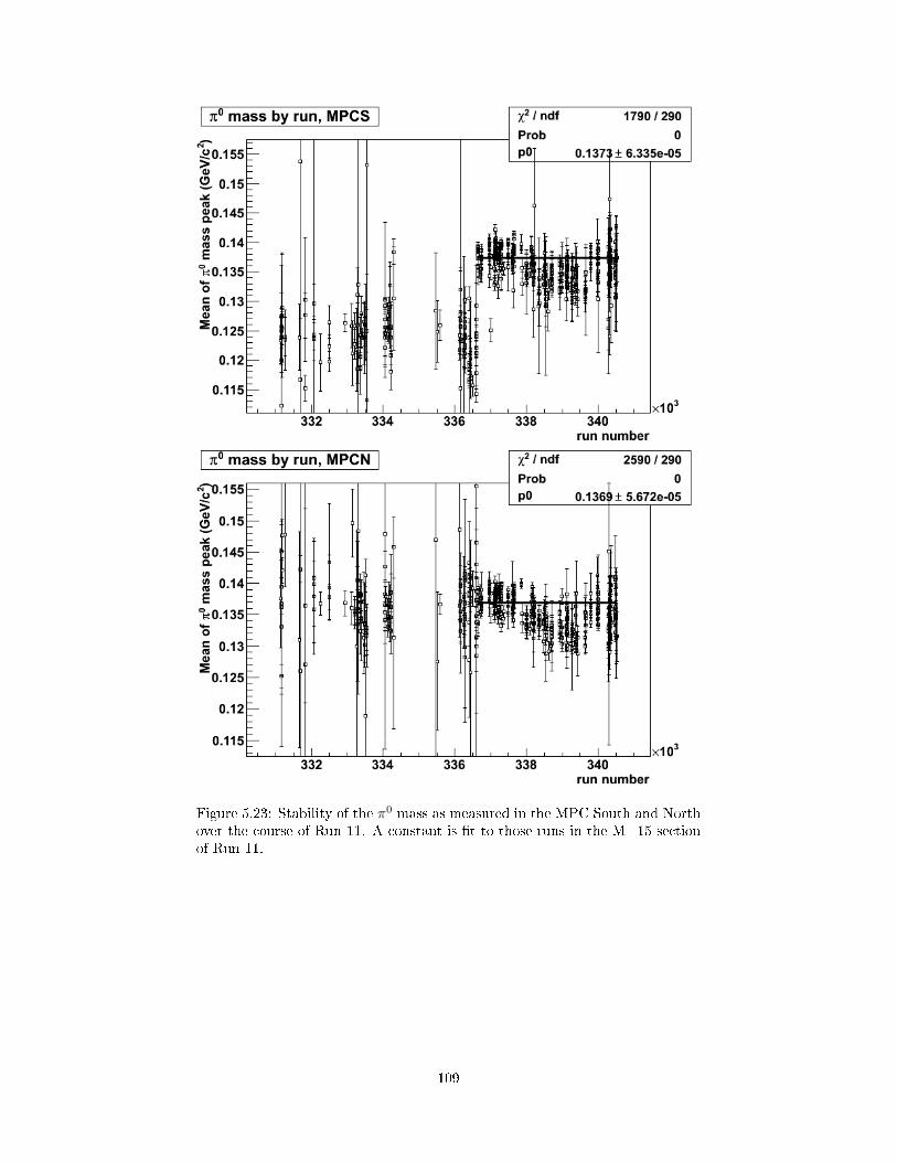
Figure 5.23: Stability of the π0 mass as measured in the MPC South and Northover the course of Run 11. A constant is �t to those runs in the M=15 sectionof Run 11.
109

Figure 5.24: Stability of the π0 width as measured in the MPC South and Northover the course of Run 11. A constant is �t to those runs in the M=15 sectionof Run 11.
First, note in Figure 5.23 the poor statistics (as evidenced by the large
error bars) and the poor quality of the calibration in general in the M=10
section of the run, before run 336636, especially in the south arm of the MPC.
These factors weigh heavily against including the M=10 section of data in the
�nal analysis. In the M=15 section of the run, the masses are comparatively
very consistent, with a noticeable drop in the π0 mass around run 339000 that
nevertheless only amounts to around a 5% �uctuation. This decline in the
110

reconstructed π0 mass appears correlated with increasing rates in RHIC around
the same time (see Figure 5.25).
Figure 5.25: Correlation between BBCwide trigger rate and reconstructed π0
mass in the MPCS (left) and MPCN (right).
I can only speculate about the nature of the correlation; it may be that the
increased rates result in a higher fraction of crossings with multiple collisions,
and the combinatorial background from clusters in the multiple collisions is not
accounted for properly when �tting the mass peak. The 5% di�erence in the
mass over the course of the M=15 section of the run is of comparable size to
the spread in π0 datamasssim.mass from tower to tower after running the iterative π0
calibration.
The mass peak widths (Figure 5.24) are more or less stable in both the M=10
and M=15 segments of the run, with a value between 30 and 35MeV/c2. The
widths are larger than those seen in Run 9 by about 10MeV/c2. The increased
widths are seen in later runs as well, so the decreased resolution may be a result
of the degradation of the detector with time or the necessity of running with
lower high-voltage settings for the best dynamic range at center-of-mass energies
of 500 or 510 GeV .
111
Chapter 6
Run 11 MPC Aclus.LL analysis
Having covered in detail the technical tasks relating to the luminosity normal-
ization for our measurement (chapter 4) as well as the calibration of the MPC
(chapter 5), we turn to the �nal physics analysis where we determine the dou-
ble longitudinal spin asymmetry in the production of electromagnetic clusters
in the MPC. The Aclus.LL analysis is similar in many respects to the ALL(ZDCBBC )
analysis, but di�erences between the MPC and the luminosity detectors provide
some additional complexity to the measurement. The main di�erences can be
explained by the fact that the MPC reports much more than the �hit or no hit�
information we typically use from the luminosity monitors; we record timing
and energy information from each of 416 channels (196 in the south arm, 220
in the north).
One complication of the luminosity scaler analysis that for multiple reasons
is not required for the MPC data is a pileup correction. We count clusters in
the MPC for this analysis, rather than simple binary single-arm or coincidence
counts. Therefore, there is no possibility of an accidental coincidence to worry
about. Also, �missing� a hit in a tower because a second collision in the same
crossing caused a hit in the same tower is unlikely on account of the segmentation
of the MPC and the low rates of high pT clusters in the MPC.
The additional information read out by the MPC compared to the ZDC and
the BBC also allows for more detailed analysis of the detector's performance.
For example, while we were restricted in our luminosity monitors to exclude
data only on the crossing or run level, we are free to also eliminate sections or
individual towers from the MPC on a run-to-run basis from our �nal analysis.
The fact that we read out energies from the MPC towers also gives us more
options in terms of detector QA since we can examine the detector response in
various energy ranges. Finally, having knowledge of cluster energies also allows
us to report the �nal asymmetry as a function of pT , which is important for
theoretical purposes as the pT gives us a handle of the kinematics of a collision
and therefore what momentum fraction of the proton is being probed.
112

6.1 Analyzing merged clusters
While the MPC can reconstruct π0's from the two clusters resulting from the
decay of the π0 to two photons, as seen in our iterative π0 calibration, restricting
our analysis to reconstructed π0's would severely limit our statistics for the
measurement as well as the kinematic range we can cover. The di�culty is that
the opening angle between the two photons resulting from a π0 decay depends
on the energy of the π0 and how the energy is distributed between the photons.
The invariant mass of a particle in the high-energy limit (where E = |p|) interms of the four momenta of its two decay products (photons in our case) is
the scaler product of those four momenta:
m2γγ = pµp
µ = E2 − p2 = 2E1E2(1− cosθ), (6.1)
where θ is the angle between the three-momenta of the two photons and E1
and E2 are their energies. As the total angular diameter of the MPC at 220 cm
is only 10◦, we use the small-angle approximation to rewrite Equation 6.1 as
m2γγ = 2E1E2
θ2
2 . We can immediately see that for the �xed mass of the π0, the
angle between the photon momenta decreases as the energy increases. We also
de�ne a total energy Etot = E1+E2 and an energy asymmetry α = |E1−E2|Etot
such
that α2 =E2
1−2E1E2+E22
E2tot
=E2
tot−4E1E2
E2tot
, so 2E1E2 =E2
tot(1−α2)
2 and Equation 6.1
becomes
m2γγ =
E2tot
2(1− α2)
θ2
2. (6.2)
Our analysis requires a minimum separation of only 2.6 cm between clusters;
however, the clusters cannot be cleanly resolved if their centers are in adjacent
towers. The clusters can be considered a merged cluster if the separation be-
tween their centers is less than 2× 2.2 cm, corresponding to an angle at 220 cm
of 0.022 radians. and a maximum α of 0.6. Plugging these values and the π0
mass of 0.135 GeV/c2 into Equation 6.2, we �nd that the highest-energy π0 we
can reconstruct has E ≈ 17GeV and a maximum pT (for clusters at the outer
edge of the MPC's acceptance) of 1.5GeV/c. If we allow the smaller cluster
separation of 2.6 cm used in the iterative π0 calibration, we can theoretically re-
construct a π0 with E ≈ 28GeV and pT ≈ 2.4GeV/c. These limits are reduced
further when considering cluster pairs with either no energy asymmetry or the
average energy asymmetry around 0.25.
The theoretical framework of pQCD is applicable only for pT > 1GeV/c
where hard interactions dominate, so we have theoretical motivation to focus
on the higher-energy merged clusters as well. While is not practical to focus
our analysis on reconstructed π0's, simulations indicate that the merged clusters
come predominantly from π0's anyway. A study of 30 million PYTHIA events at√s = 500GeV showed that around 80% of merged clusters above pT = 1GeV/c
arise from π0 decay, with smaller contributions from merged clusters from η
meson decay, direct photons, and charged hadrons[65]. The cluster decomposi-
113

tion, showing the fraction of clusters arising from the various contributions as
a function of pT as determined from simulation, is shown in Figure 6.1.
Figure 6.1: Cluster decomposition results from PYTHIA and GEANT at√s =
500GeV .
6.1.1 Single-tower background
There is a background signal that dominates the MPC-triggered data for high-
energy clusters that is known as the single-tower background (Figure 6.2). The
background consists of clusters that do not have any reasonable lateral extent;
instead, what appears to be an unphysically large energy is deposited in a single
tower, with little or no energy in surrounding towers. The energy spectra of these
clusters is �at as well rather than falling o� as a power law at high energies as
would be expected for particles produced in a pp collision. This signal is thought
to be produced by neutrons from interactions between high-energy particles and
steel support structures in PHENIX. These neutrons do not initiate showers
in the PbWO4 crystals, but occasionally they can interact directly with the
silicon in the APDs, kicking out a proton in a nuclear reaction and initiating an
avalanche that in itself is indistinguishable from the avalanche resulting from
scintillation light in the crystals. While the neutrons themselves have small
energies on the order of a hundred MeV, they produce a signal corresponding to
what a particle with tens of GeV of energy would yield through electromagnetic
showering in the detector.
114

Figure 6.2: MPC 4x4a and 4x4b triggers. The spectrum for the 4x4b trigger isin�ated by the presence of the single-tower background which is the dominantsource of clusters with energy above 80GeV or pT above 5GeV (see Figure 6.4).
We attempt to eliminate the single-tower background through a number of
cuts on cluster parameters. These cuts all generally key on the fact that the
background does not involve a shower, so there is no lateral spread of energy
(unless by coincidence with another cluster). One simple cut would be to simply
remove clusters with fewer than a certain number of towers. In the past, analyz-
ers have removed clusters with fewer than three towers, though it seems this can
be pushed further since many of the clusters with only two towers nevertheless
appear normal by other measures. A more direct measure of the spatial extent
of the shower is the dispersion, and requiring the dispersion to be larger than
0.001 essentially selects those clusters with a multiplicity of 1. In terms of the
energy distribution, we know that a typical cluster centered at the center of a
crystal will deposit around 90% of its energy in that crystal and 10% in other
crystals. Single-tower background clusters will claim even larger fractions of the
cluster energy in their central towers, so requiring that Ecentral tower
Eclusteris smaller
than some fraction1 provides another overlapping cut against the background.
Finally, as the position of a cluster's center is calculated as an energy-weighted
average of the locations of towers in the cluster, clusters with one dominant
tower will have their positions entirely determined by the one tower. This po-
1In calculating total cluster energies, only towers with > 2% of the total energy of towersin the cluster contribute to the cluster energy. A factor of 1
0.918is applied to the sum of
the individual tower energies to compensate, meaning that for a truly single tower cluster,EcentEclus
= 0.918. A hypothetical electromagnetic shower depositing 90% of its energy in one
tower and the other 10% in the eight surrounding towers will in contrast have EcentEclus
≈ 0.83.
115

sition shows up clearly as a single-bin spike in a histogram of cluster positions
within a single tower. The actual width of the spike is even much smaller than
shown in the histogram, and we can exclude clusters at the position of the spike.
Figure 6.3: The distribution of cluster r for channel 4 shows a spike between11.7 and 11.8 cm corresponding to the single tower background.
Unfortunately, the chances of at least one tower reporting a high-energy
signal consistent with the single tower background are much higher than the
chances of a tower recording a hit from a particle with the same high energy.
As a result, there is a signi�cant contamination of the triggered data set by the
background signal, and perhaps as few as 5-10% of the clusters we see above
80 GeV in energy are of interest to us. The MPC4x4b trigger is especially
hit hard owing to its higher threshold and correspondingly low rates of �real�
triggers. We show the contamination of the total triggered data sample due to
the single-tower background as well as the spectra after the background clusters
are removed in Figure 6.4.
116

Figure 6.4: E�ect of single tower background cut on cluster pT spectrum. Thereare around ten times as many clusters removed by our single tower backgroundcuts than there are good clusters for pT > 5GeV .
6.1.2 MPC QA
Before computing the �nal cluster yields and asymmetries with data from the
MPC, we must determine which runs and crossings are suitable for inclusion
in our analysis. A number of runs and crossings are already excluded due to
quality checks on data from the BBC and ZDC scalers. We summarize excluded
runs and crossings here.
6.1.2.1 Run-level QA
We carry out checks similar to the ones we employed in the scaler data QA on
a run-by-run level with the MPC data.
Missing data Of the 432 runs marked for physics use in the data acquisition
database, 10 runs were not processed to generate the MPC data �les.
MPC calibration di�culties Possibly due to the lower high-voltage settings
on the MPC APDs in the M=10 section of Run 11 (before run 336636), or
possibly in part due to the same beam stability issues that caused di�culties
in analyzing the BBC and ZDC data before run 336000, we have been unable
at this point to converge on a �nal set of gains for this section of Run 11. Our
measurements of tower and cluster counts per trigger and bunch shu�ing widths
also show wide variations in this early part of Run 11 that are not present in
the M=15 section. For these reasons, we exclude the portion of Run 11 where
117

the MPC is running at the M=10 setting, as well as the �rst �ll at the M=15
setting. Most of this data is excluded due to the BBC and ZDC QA cuts as
well.
PHENIX data acquisition problems Four runs were aborted very early
on due to problems with the data acquisition system; data collected from these
runs is unreliable.
Abort gap alignment For each run, we check that crossings 111 to 119 are
empty, as no collisions occur in these crossings. A crossing shift for each run had
been determined previously by analyzers in PHENIX's Spin Physics Working
Group that corrects the crossing numbers reported in the original data. After
applying the crossing shift, all runs were aligned as expected. However, eight
runs had an abort gap that was one crossing too long as well as sporadic pairs
of empty crossings throughout the rest of the �rst 110 crossings, so we exclude
these runs from our analysis.
6.1.2.2 Crossing-level QA
To �nd outlying crossings that should be excluded, we looked at the number of
clusters in each crossing that pass all of our analysis cuts. We �t a constant
to these values from crossing 0 to crossing 110 and use ROOT's LTS regression
method to only include 85% of the crossings (so the empty-full crossings, for
example, do not have a disproportionate e�ect on the �t). Any crossing with
fewer clusters than 0.5× the run average is �agged as bad. The number of good
clusters for each crossing for a typical run along with the constant �t is shown
in Figure 6.5.
118
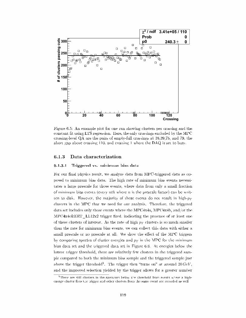
Figure 6.5: An example plot for one run showing clusters per crossing and theconstant �t using LTS regression. Here, the only crossings excluded by the MPCcrossing-level QA are the pairs of empty-full crossings at 38,39,78, and 79, theabort gap above crossing 110, and crossing 1 where the DAQ is set to busy.
6.1.3 Data characterization
6.1.3.1 Triggered vs. minimum bias data
For our �nal physics result, we analyze data from MPC-triggered data as op-
posed to minimum bias data. The high rate of minimum bias events necessi-
tates a large prescale for those events, where data from only a small fraction
of minimum bias events (every nth where n is the prescale factor) can be writ-
ten to disk. However, the majority of these events do not result in high-pT
clusters in the MPC that we need for our analysis. Therefore, the triggered
data set includes only those events where the MPC4x4a, MPC4x4b, and/or the
MPC4x4c&ERT_LL12x2 trigger �red, indicating the presence of at least one
of these clusters of interest. As the rate of high-pT clusters is so much smaller
than the rate for minimum bias events, we can collect this data with either a
small prescale or no prescale at all. We show the e�ect of the MPC triggers
by comparing spectra of cluster energies and pT in the MPC for the minimum
bias data set and the triggered data set in Figure 6.6. At energies below the
lowest trigger threshold, there are relatively few clusters in the triggered sam-
ple compared to both the minimum bias sample and the triggered sample just
above the trigger threshold2. The trigger then �turns on� at around 20GeV ,
and the improved selection yielded by the trigger allows for a greater number
2There are still clusters in the spectrum below the threshold from events where a high-energy cluster �res the trigger and other clusters from the same event are recorded as well
119

of high-energy clusters to be collected, given bandwidth limitations, compared
to the minimum bias trigger.
(a) Cluster energy spectra for minimum bias and triggered data.
(b) Cluster pT spectra for minimum bias and triggered data.
Figure 6.6: Comparison of cluster spectra in minimum bias and triggered data.
6.1.3.2 BBC vertex distribution
Figure 6.7 contains the BBC collision vertex distributions for MPC-triggered
events. For each event, we also �nd the highest-energy cluster in the MPC
(generally the one responsible for �ring the trigger), and we separate the overall
120

vertex distribution into two distributions based on whether the leading cluster
was in the north or south arm. The distribution for the MPCN is larger as
expected due to its larger acceptance. The collision vertex locations are biased
slightly towards the arm containing the leading cluster, as there is also a vertex-
dependent acceptance e�ect in the MPC; for a given angle of a particle leaving
the collision and the beam axis, more particles will hit the MPC if the vertex is
closer to the detector.
Figure 6.7: Distribution of collision vertices as determined by the BBC forMPC-triggered events.
6.2 Merged cluster identi�cation
As discussed previously, for our �nal asymmetries, we consider single high-
energy clusters in the MPC, the majority of which arise from overlapping pairs
of clusters from π0 decay. We apply cuts to clusters in the MPC to maximize
the number of merged clusters in the analysis while minimizing the contribution
from clusters from unmerged π0's and the single tower background. The cuts
used are the following:
• Ecluster > 15GeV
• pT, cluster > 1.5GeV/c
• 12 cm < rcluster < 19 cm
• Central tower not in warn map
• ADC not over�owed
121

• TDC not over�owed
• dispersion > 0.0005 cm2
• At least three towers in the cluster
• Cluster r not in excluded tower-by-tower spike
6.3 Calculating the asymmetries
Recall the de�nitions for the parity-violating single-spin asymmetries AL,b(y) we
use as a crosscheck and the double longitudinal spin asymmetry ALL:
Aclus.L,b(y) =1
Pb(y)
N+clus. −RN
−clus.
N+clus. +RN+
clus.
,
Aclus.LL =1
|PbPy|N++clus. −RN
+−clus.
N++clus. +RN+−
clus.
. (6.3)
As input to the asymmetry calculation for a given run, we need blue and yellow
beam polarization values, cluster yields, and a measurement of relative lumi-
nosity. The blue and yellow beam polarizations can be found in a database
provided by RHIC Spin[60] as in the relative luminosity analysis. We count
clusters that pass all of our analysis cuts in pT bins of 1.5-2.0, 2.0-2.5, 2.5-3.0,
3.0-4.0, 4.0-5.0, 5.0-6.0, 6.0-7.0, 7.0-8.0, and 8.0-12.0 GeV/c. The scaler counts
for determining relative luminosity come from the BBCwide trigger, and the
cluster yields and scaler yields are sorted by bunch according to the blue and
yellow beam helicities (hbhy), where the helicities can be + or −. For Aclus.LL ,
crossings are grouped into same-sign (++ or +−) crossings and opposite-sign
(+− or −+) crossings, excluding crossings removed by data quality cuts (the
same crossings are excluded when calculating both the scaler and cluster yields).
For the single spin asymmetries, Aclus.L,b(y), we consider only the helicity of the blue
or yellow bunch in grouping crossings. We calculate an asymmetry for each run
individually, and the resulting run-by-run asymmetries are �t with a constant
to determine the �nal overall asymmetry. We calculate asymmetries separately
for even and odd crossings (due to slightly di�erent thresholds in the separate
trigger circuits for even and odd crossings) and for the north and south arms
of the MPC. These are checked for consistency and then combined for the �nal
result.
6.4 Single-spin asymmetries Aclus.L,b(y)
We calculate Aclus.L,b(y) separately for even and odd crossings, blue and yellow
beam, and the north and south arms of the MPC. An example of a �t of the
run-by-run asymmetry to a constant is shown in Figure 6.8.
122

Figure 6.8: Aclus.L,b (blue beam) by run for clusters in the MPC South in the lowestpT bin from even crossings only.
Figure 6.9: AclusterL,b(y) vs. pT for the blue (yellow) beam for clusters in the northand south arms of the MPC.
We also show Aclus.L vs. pT results for the blue and yellow beams and clus-
ters in the MPCS and MPCN in Figure 6.9. We see reasonable numbers for
χ2/NDF, and the asymmetries (given by the �t parameters) are consistent
with zero as expected due to the invariance of QCD interactions under a parity
transformation. That the single-spin asymmetries are consistent with zero puts
123

a limit on the size of possible false asymmetries
6.5 Double longitudinal spin asymmetry, Aclus.LL
We present in this section our results for Aclus.LL from the triggered data set, for
even and odd crossings and the north and south arms of the MPC. As for the
single-spin asymmetry results, we only include a sample plot of ALL vs. run
number ( 6.10a), the asymmetries vs. pT separated by arm and even/odd cross-
ings ( 6.10b), and a table of the results for those asymmetries (Table 6.1); the
complete collection of plots can be found in Appendix B. We �nd asymmetries
that are consistent over the course of Run 11 without any time-dependent ef-
fects, and the values of χ2/NDF for the constant �ts to the plots of asymmetry
vs. run number are reasonable as well.
124
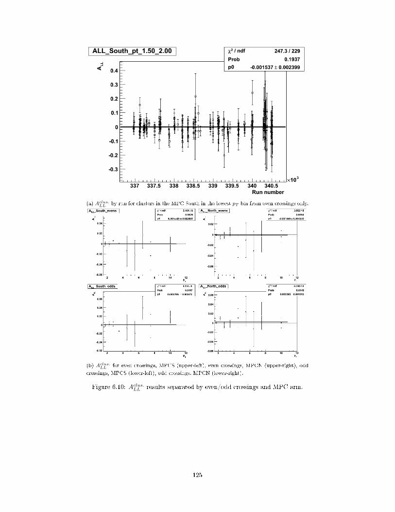
(a) Aclus.LL by run for clusters in the MPC South in the lowest pT bin from even crossings only.
(b) Aclus.LL for even crossings, MPCS (upper-left), even crossings, MPCN (upper-right), odd
crossings, MPCS (lower-left), odd crossings, MPCN (lower-right).
Figure 6.10: Aclus.LL results separated by even/odd crossings and MPC arm.
125

Table 6.1: AclusterLL results for MPC-triggered data
pmin.T pmax.T Arm Crossings AclusterLL δAclusterLL (stat.) χ2/NDF
1.5 2 South evens 8.74E-05 0.00350374 219.84/215
1.5 2 North evens 0.000589329 0.00236312 209.947/215
1.5 2 South odds -0.00105821 0.00348314 223.497/215
1.5 2 North odds 0.000911657 0.00235704 237.524/215
2 2.5 South evens -0.000572485 0.00579321 197.695/215
2 2.5 North evens -0.00464812 0.00377094 191.88/215
2 2.5 South odds 0.00143051 0.00577246 223.396/215
2 2.5 North odds 0.00924482 0.00375744 205.197/215
2.5 3 South evens 0.00602013 0.00933998 186.998/215
2.5 3 North evens -0.00166943 0.00619408 239.691/215
2.5 3 South odds 0.00639768 0.00931184 177.114/215
2.5 3 North odds -0.00467624 0.00614869 211.79/215
3 4 South evens 0.0008295 0.0126835 187.851/215
3 4 North evens 0.00532805 0.00862869 213.868/215
3 4 South odds -0.0146179 0.0125706 207.43/215
3 4 North odds -0.00184115 0.00853786 242.726/215
4 5 South evens -0.0141161 0.0296622 251.249/215
4 5 North evens -0.0227218 0.0206473 242.995/215
4 5 South odds -0.00629458 0.0292019 267.814/215
4 5 North odds 0.0103657 0.0204816 215.677/215
5 6 South evens -0.0230577 0.0295705 264.104/214
5 6 North evens -0.0108052 0.0325265 196.98/214
5 6 South odds -0.0203544 0.0294782 210.414/214
5 6 North odds 0.0245385 0.0324754 219.451/215
6 7 South evens 0.0180156 0.0267388 243.567/214
6 7 North evens -0.0310115 0.0373504 255.458/212
6 7 South odds 0.0394927 0.0266028 195.497/213
6 7 North odds -0.0127945 0.0373464 229.983/213
7 8 South evens -0.0237393 0.0273027 209.183/214
7 8 North evens -0.00361396 0.0295606 237.791/214
7 8 South odds -0.00270692 0.027246 186.997/214
7 8 North odds 0.0150494 0.0294366 207.397/215
8 12 South evens -0.00122043 0.014753 191.961/215
8 12 North evens -0.00399833 0.0110609 223.818/215
8 12 South odds 0.0184251 0.0146121 233.835/215
8 12 North odds 0.000360406 0.0110379 268.267/215
126

6.5.1 Consistency between even and odd crossings and
MPCS and MPCN results
To check for consistency between the asymmetries in each pT bin between even
and odd crossings and north and south arms, we employ a Student's T-test. For
each pT bin, we calculate a T-score,
T − score =ALL,1(pT )−ALL,2(pT )√
(δALL,1(pT ))2 + (δALL,2(pT ))2, (6.4)
that gives the separation between the asymmetries in units of the statistical
error. We then plot the distribution of T-scores, which is expected to follow a
Student's t-distribution.
The bin-by-bin T-scores and the distributions are shown in Figure 6.11.
We see no systematic di�erence between the asymmetries calculated from the
even crossings versus the odd crossings, and the asymmetries in the MPCS and
MPCN are consistent as well.
Figure 6.11: T-tests between asymmetries for even and odd crossings in theMPCS (left), even and odd crossings in the MPCN (middle), and the �nal(even/odd combined) MPCS and MPCN ALL (right).
6.5.2 Aclus.LL by spin pattern
We also calculate Aclus.LL separately for the four spin patterns used in Run 11 to
check for systematic e�ects that depend on the sequencing of bunch helicities
in RHIC. For each of the four asymmetries, we perform the T-test described in
the previous section and combine the asymmetries from even and odd crossings
and north and south arms (Figure 6.12); again, we see nothing unusual in the
T-scores. Finally, we look for discrepancies between patterns by performing T-
tests between the two SOOS-type patterns P0 and P3, between the two OSSO-
type patterns P1 and P2, and the between the combined SOOS and OSSO
asymmetries. These three T-tests yield 9 T-scores each, and the distribution of
all T-scores from the tests are plotted in one histogram (Figure 6.13). The �nal
asymmetries for each pattern are shown in Figure 6.14. The asymmetries from
127

the four patterns show good agreement with one another, though pattern P0 is
negative and slightly further from 0 (at 1.5σ) compared to the other patterns.
Figure 6.12: Compilation of T-tests for the four spin patterns. Each row repre-sents one pattern, ordered sequentially with P0 at the top. The columns are thesame tests shown in the previous section (MPCS even/odd, MPCN even/odd,MPCS/MPCN).
128

Figure 6.13: Combined T-scores from three T-tests, checking the consistencybetween patterns 0 and 3, patterns 1 and 2, and the combined asymmetry frompatterns 0 and 3 and the combined asymmetry from patterns 1 and 2.
Figure 6.14: Aclus.LL calculated separately for each of the four spin patterns. The�t parameters and colors corresponding to the patterns are listed across the topof the plot, starting with P0.
129

6.5.3 Bunch shu�ing
We again use the bunch shu�ing method to check for errors causing a system-
atic o�set of our calculated asymmetries and to check the accuracy of the size
of our statistical errors. We randomize the beam helicities for each crossing and
recalculate ALL for each pT bin. This process is repeated 10,000 times, and
we plot the distribution of ALL/δALL in each pT bin. The shu�ing procedure
ensures that the average e�ective beam polarization over the 10,000 shu�es
is zero, so we should �nd that the mean of the error-normalized asymmetries
should be zero. The width of the distribution should be approximately one if
the statistical uncertainty δALL accurately re�ects the spread we would hypo-
thetically see if we could repeat our asymmetry measurement 10,000 times. We
demonstrate in Figure 6.15 that the shu�ed asymmetry distributions conform
to expectations and do not point to problems with our calculations of Aclus.LL
or its uncertainty. The means of the distributions lie near 0 (within the un-
certainties of the Gaussian �ts), and the widths of the distributions are around
1.02.
Figure 6.15: Bunch shu�ing results for Aclus.LL for clusters in the MPCS, allcrossings.
130

6.5.4 Final results for Aclus.LL (MPC)
Having demonstrated that we calculate consistent asymmetries in the north and
south arms and in even and odd crossings, we statistically combine the results
to determine our �nal result for Aclus.LL in the MPC. First, the even and odd
crossings are combined to give Aclus.LL for the north and south arms, and then
the results from the north and south arms are combined. The resulting �nal
asymmetry is shown in Figure 6.16, and the data points are given in Table 6.2.
We see that the overall asymmetry is consistent with zero as are the asymmetries
in each pT bin. However, the statistical uncertainties, even in the lowest pT bins,
are on the order of 10−3, meaning we are not sensitive to the small asymmetry
we are looking for which is not expected to be larger than 5 × 10⁻⁴ or so (see
subsection 3.2.3).
Figure 6.16: Final Aclus.LL (MPC) by pT at√s = 500GeV . The uncertainty on
the polarization measurement leads to an overall vertical scale uncertainty of6.6%. The systematic uncertainty from the relative luminosity measurement of2× 10−5 is not shown here as it is dwarfed by the statistical uncertainties. Thepoint in each pT bin is plotted at the average pT for the bin.
131

Table 6.2: Final bin-by-bin results for Aclus.LL (MPC) at√s = 500GeV . Units
of pT are GeV/c.
pmin.T pmax.T < pT > Aclus.LL (MPC) δAclus.LL (stat.)
1.5 2.0 1.71 0.000362416 0.00138283
2.0 2.5 2.21 0.00176058 0.00223072
2.5 3.0 2.71 -0.000323252 0.00363911
3.0 4.0 3.35 -0.00103407 0.00501924
4.0 5.0 4.40 -0.00738965 0.0119193
5.0 6.0 5.50 -0.00877294 0.0154528
6.0 7.0 6.51 0.0116827 0.0153475
7.0 8.0 7.52 -0.0044637 0.0141605
8.0 12.0 10.03 0.00198615 0.00624274
132

Chapter 7
Conclusions and outlook
With the ALL measurements with the MPC, PHENIX will provide data to
global QCD analyses that can constrain ∆g(x) for smaller x than is accessed by
central arm measurements, helping to answer the question of how much spin in
total the gluons contribute to the proton spin of 1/2. The Run 9 measurements
of the forward cluster ALL at√s = 200GeV and
√s = 500GeV [65] and this
measurement at√s = 500GeV show asymmetries consistent with zero; how-
ever, the expected asymmetries according to our simulations were small to begin
with, even for signi�cant gluon polarizations, and these are not yet conclusively
ruled out. In this thesis, we have shown how we reduced the uncertainty of
our relative luminosity determination, the leading systematic uncertainty, from
1.3 × 10⁻³ to 2 × 10⁻⁵. With this small systematic uncertainty, analysis of
a much larger data set from 2013 will provide the statistical precision needed
to distinguish between no asymmetry or a possible small asymmetry at forward
rapidity, reducing the wide array of functional forms of ∆g(x) that are presently
consistent with the DSSV analysis. This is crucial for constraining the gluon
contribution to the proton spin for x < 0.05, where current �ts allow for glu-
ons in the small-x region alone to have total helicity ranging from more than12~(the total spin of the proton) to 1
4~ in the opposite direction of the proton's
spin. The potential impact of the ALL measurements in the MPC was discussed
with Rodolfo Sassot of the DSSV group at the 2014 PHENIX SpinFest anal-
ysis meeting in Urbana. Following the discussion, Rodolfo produced the plot
shown in Figure 7.1 to quantify the importance of the MPC analyses to our
understanding of the gluon polarization at low x. While PHENIX and STAR
continue to provide data improving constraints on the gluon polarization for
x > 0.02, the forward measurements will be the �rst to provide information on
the gluon polarization for x < 0.01 as represented by the signi�cant narrowing
of the uncertainty band in Figure 7.1 once projected data from the forward
measurements through 2015 are included.
The �nal word on gluon spin, however, is likely to come from a proposed
electron-ion collider (EIC)[66]. The EIC would be the world's �rst polarized
electron-proton collider and would run at extremely high luminosities, and as
Figure 7.2 shows, the range of center-of-mass energies and Q2 would be su�cient
to constrain ∆g(x) even below x ≈ 10−4.
133

Figure 7.1: Here we show the projected impact of forward measurement of ALLin the MPC through 2015 as well as similar measurements from STAR usingtheir forward electromagnetic calorimeter[44]. In each bin of x, the contribu-tion to the total gluon polarization from that range of x is plotted along withuncertainty bands corresponding to the 90% con�dence interval. Results areshown for the original DSSV analysis including only RHIC data through 2006,the updated DSSV 14 analysis including RHIC data through 2009, and a projec-tion that re�ects the impact of data from simulations representing RHIC datathrough 2015 (with the forward measurements).
134

Figure 7.2: Plots showing the projected impact of an electron-ion collider on ourknowledge of ∆g(x). The plot on the left shows the kinematic ranges coveredby the EIC, while the plot on the right shows the projected impact on theuncertainty bands of the DSSV �t[66].
135

Appendix A
Runs used in �nal analysis
The runs passing the scaler data QA cuts and entering into the asymmetry
calculations were the following:
336155 336156 336157 336158 336159 336160 336285 336286 336502 336596
336597 336598 336601 336603 336604 336609 336610 336962 336963 336964
336968 336969 336971 337113 337115 337116 337117 337118 337119 337120
337121 337122 337123 337131 337133 337140 337141 337142 337143 337217
337219 337220 337221 337222 337234 337236 337237 337238 337239 337240
337242 337290 337291 337292 337293 337302 337359 337360 337494 337495
337496 337497 337498 337499 337500 337618 337619 337620 337621 337622
337624 337627 337629 337642 337643 337645 337648 337649 337650 337651
337652 337653 337864 337865 337877 338003 338005 338006 338008 338009
338010 338012 338097 338203 338208 338209 338210 338211 338212 338213
338349 338350 338351 338352 338353 338354 338355 338490 338491 338492
338493 338494 338496 338535 338536 338539 338542 338543 338544 338545
338546 338613 338677 338920 338922 338925 338926 338927 338928 338992
338993 338994 338995 339118 339120 339122 339123 339124 339125 339127
339129 339130 339134 339135 339136 339138 339139 339140 339141 339142
339144 339238 339269 339273 339274 339277 339278 339364 339365 339367
339375 339376 339430 339432 339570 339572 339580 339583 339587 339591
339639 339640 339641 339646 339647 339648 339649 339795 339797 339801
339803 339805 339981 339982 339984 339985 339989 339992 339993 339994
339996 339999 340000 340006 340009 340273 340285 340287 340289 340296
340306 340308 340310 340312 340314 340315 340316 340321 340324 340326
340327 340334 340335 340336 340337 340342 340343 340344 340349 340367
340368 340369 340371 340476 340477 340478 340486 340489 340490 340491
340492 340493 340495 340496 340506 340508 340511 340512 340513.
136

Appendix B
Asymmetry plots
B.1 AL(ZDCBBC )
Figure B.1: AL,b(ZDCBBC ) (blue beam) vs. run for all crossings.
137

Figure B.2: AL,b(ZDCBBC ) (blue beam) vs. run for all crossings, separated by spin
pattern.
Figure B.3: AL,y(ZDCBBC ) (yellow beam) vs. run for all crossings.
138

Figure B.4: AL,y(ZDCBBC ) (yellow beam) vs. run for all crossings, separated byspin pattern.
B.2 ALL(ZDCBBC )
Figure B.5: ALL(ZDCBBC ) vs. run for all crossings.
139
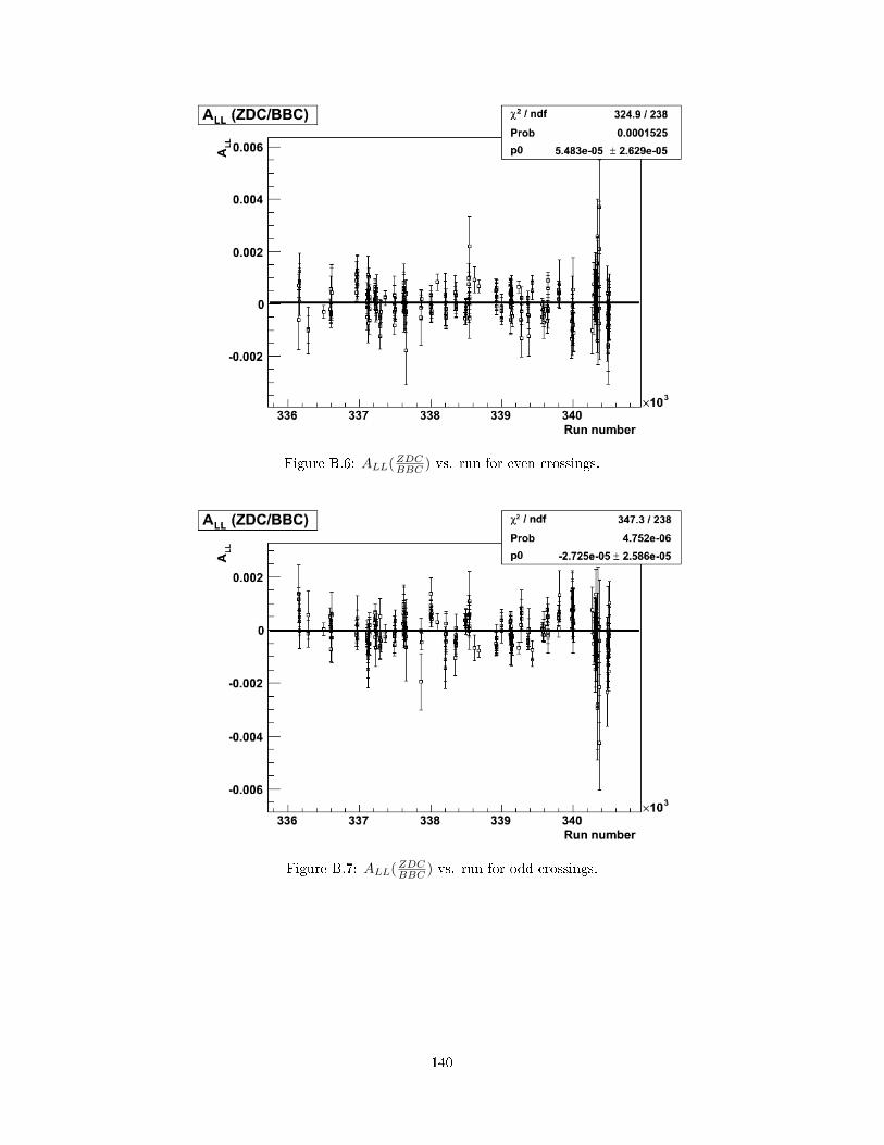
Figure B.6: ALL(ZDCBBC ) vs. run for even crossings.
Figure B.7: ALL(ZDCBBC ) vs. run for odd crossings.
140
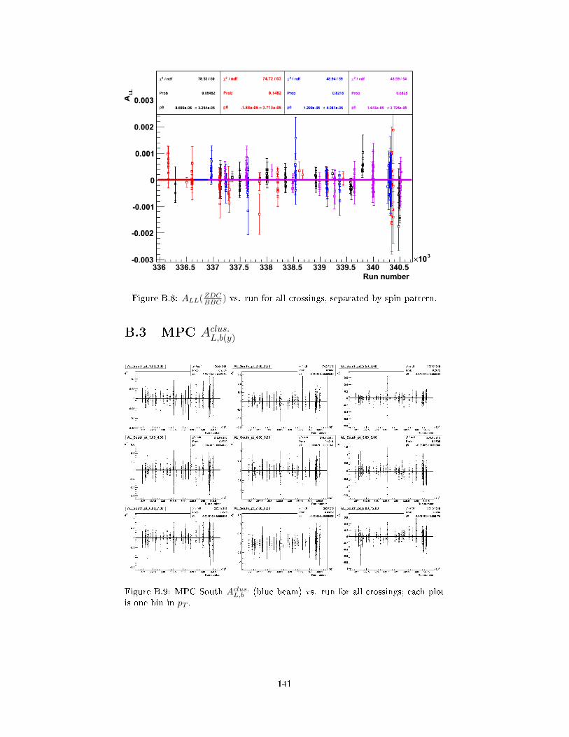
Figure B.8: ALL(ZDCBBC ) vs. run for all crossings, separated by spin pattern.
B.3 MPC Aclus.L,b(y)
Figure B.9: MPC South Aclus.L,b (blue beam) vs. run for all crossings; each plotis one bin in pT .
141
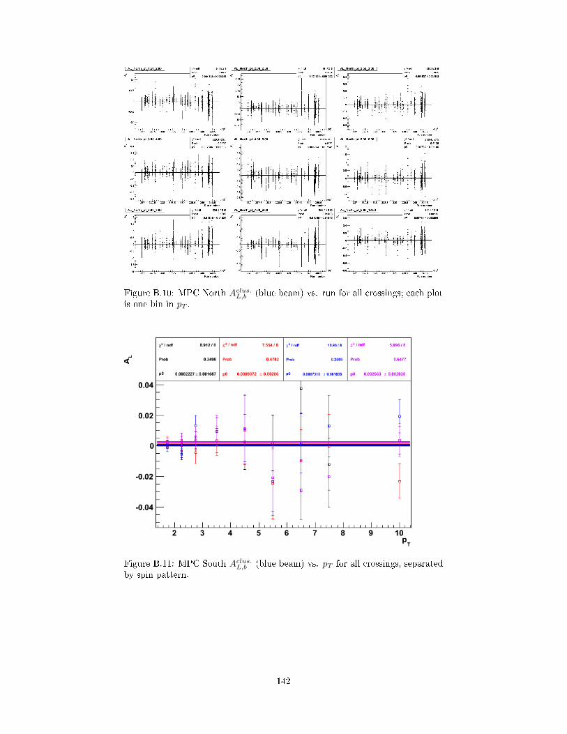
Figure B.10: MPC North Aclus.L,b (blue beam) vs. run for all crossings; each plotis one bin in pT .
Figure B.11: MPC South Aclus.L,b (blue beam) vs. pT for all crossings, separatedby spin pattern.
142

Figure B.12: MPC North Aclus.L,b (blue beam) vs. pT for all crossings, separatedby spin pattern.
Figure B.13: MPC South Aclus.L,y (yellow beam) vs. run for all crossings; eachplot is one bin in pT .
143

Figure B.14: MPC North Aclus.L,y (yellow beam) vs. run for all crossings; eachplot is one bin in pT .
Figure B.15: MPC South Aclus.L,y (yellow beam) vs. pT for all crossings, separatedby spin pattern.
144
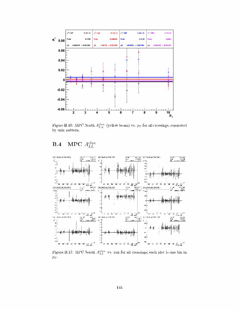
Figure B.16: MPC North Aclus.L,y (yellow beam) vs. pT for all crossings, separatedby spin pattern.
B.4 MPC Aclus.LL
Figure B.17: MPC South Aclus.LL vs. run for all crossings; each plot is one bin inpT .
145

Figure B.18: MPC North Aclus.LL vs. run for all crossings; each plot is one bin inpT .
Figure B.19: MPC South Aclus.LL vs. pT for all crossings, separated by spinpattern.
146

Figure B.20: MPC North Aclus.LL vs. pT for all crossings, separated by spinpattern.
Figure B.21: MPC North and South combined Aclus.LL vs. pT for all crossings,separated by spin pattern.
147

B.4.1 MPC Aclus.LL bunch shu�ing
Figure B.22: Bunch shu�ing results for Aclus.LL in the MPC South for all cross-ings; each plot is one pT bin.
148

Figure B.23: Bunch shu�ing results for Aclus.LL in the MPC North for all cross-ings; each plot is one pT bin.
149
Bibliography
[1] Joseph John Thomson. XL. Cathode rays. The London, Edinburgh, andDublin Philosophical Magazine and Journal of Science, 44(269):293�316,1897.
[2] Joseph John Thomson. XXIV. On the structure of the atom: an investi-gation of the stability and periods of oscillation of a number of corpusclesarranged at equal intervals around the circumference of a circle; with ap-plication of the results to the theory of atomic structure. The London,Edinburgh, and Dublin Philosophical Magazine and Journal of Science,7(39):237�265, 1904.
[3] Hans Geiger and Ernest Marsden. On a di�use re�ection of the α-particles.Proceedings of the Royal Society of London. Series A, Containing Papersof a Mathematical and Physical Character, 82(557):495�500, 1909.
[4] Ernest Rutherford. LXXIX. The scattering of α and β particles by mat-ter and the structure of the atom. The London, Edinburgh, and DublinPhilosophical Magazine and Journal of Science, 21(125):669�688, 1911.
[5] Ernest Rutherford. LVII. The structure of the atom. The London,Edinburgh, and Dublin Philosophical Magazine and Journal of Science,27(159):488�498, 1914.
[6] Ernest Rutherford. LIV. Collision of α particles with light atoms. IV. Ananomalous e�ect in nitrogen. The London, Edinburgh, and Dublin Philo-sophical Magazine and Journal of Science, 37(222):581�587, 1919.
[7] Otto Stern. The method of molecular rays. Nobel lecture., 1946.http://www.nobelprize.org/nobel_prizes/physics/laureates/
1943/stern-lecture.pdf.
[8] Martin Breidenbach, Jerome I Friedman, Henry W Kendall, et al. Observedbehavior of highly inelastic electron-proton scattering. Physical ReviewLetters, 23(16):935, 1969.
[9] Richard P Feynman and Murray Gell-Mann. Theory of the Fermi interac-tion. Physical Review, 109(1):193, 1958.
[10] M. Gell-Mann. A schematic model of baryons and mesons. Physics Letters,8(3):214�215, Feb 1964.
[11] George Zweig. An SU (3) model for strong interaction symmetry and itsbreaking. Version 1, 1964. http://cds.cern.ch/record/570209/files/
CERN-TH-412.pdf.
[12] John Ellis. The discovery of the gluon. International Journal of ModernPhysics A, 29(31), 2014.
150

[13] Xiangdong Ji, Jian-Hui Zhang, and Yong Zhao. Justifying the naive par-tonic sum rule for proton spin. Physics Letters B, 743:180�183, 2015.
[14] David Gri�ths. Introduction to elementary particles. John Wiley & Sons,2008.
[15] Francis Halzen and Alan D Martin. Quark & Leptons: An IntroductoryCourse In Modern Particle Physics. John Wiley & Sons, 2008.
[16] Bogdan Povh, Martin Lavelle, Klaus Rith, Christoph Scholz, and FrankZetsche. Particles and nuclei: an introduction to the physical concepts.Springer Science & Business Media, 2008.
[17] Gerry Bunce, Naohito Saito, Jacques So�er, and Werner Vogelsang.Prospects for spin physics at RHIC. Annual Review of Nuclear and ParticleScience, 50(1):525�575, Dec 2000.
[18] Werner Vogelsang. The spin structure of the nucleon. Journal of PhysicsG: Nuclear and Particle Physics, 34(7):S149, 2007.
[19] V.N. Gribov and L.N. Lipatov. Deep inelastic e p scattering in perturbationtheory. Sov.J.Nucl.Phys., 15:438�450, 1972.
[20] Guido Altarelli and G Parisi. Asymptotic freedom in parton language.Nuclear Physics B, 126(2):298�318, 1977.
[21] YL Dokshitzer. Calculation of the structure functions for deep inelasticscattering and e+ e- annihilation by perturbation theory in quantum chro-modynamics. Sov. Phys. JETP, 46(4):641, 1977.
[22] Daniel de Florian, Rodolfo Sassot, Marco Stratmann, and Werner Vogel-sang. Extraction of Spin-Dependent Parton Densities and Their Uncertain-ties. Phys.Rev., D80:034030, 2009.
[23] M Glück, E Reya, M Stratmann, and W Vogelsang. Models for the polar-ized parton distributions of the nucleon. Physical Review D, 63(9):094005,2001.
[24] Kieran Peter Boyle. Measurements of the double helicity asymmetry inpion production in proton collisions s**(1/2) = 200-GeV and the resultingconstraints on the polarized gluon distribution in the proton. PhD thesis,SUNY, Stony Brook, 2008-05.
[25] J.F. Owens, A. Accardi, and W. Melnitchouk. Global parton distributionswith nuclear and �nite-Q2 corrections. Phys.Rev., D87(9):094012, 2013.
[26] H Hahn, E Forsyth, H Foelsche, et al. The RHIC design overview. Nu-clear Instruments and Methods in Physics Research Section A: Accelerators,Spectrometers, Detectors and Associated Equipment, 499(2):245�263, 2003.
[27] M Harrison, T Ludlam, and S Ozaki. RHIC project overview. Nuclear In-struments and Methods in Physics Research Section A: Accelerators, Spec-trometers, Detectors and Associated Equipment, 499(2):235�244, 2003.
[28] MJ Tannenbaum. Highlights from BNL-RHIC. arXiv preprintarXiv:1201.5900, 2012.
[29] Run Overview of the Relativistic Heavy Ion Collider. http://www.
rhichome.bnl.gov/RHIC/Runs/.
151
[30] I Alekseev, C Allgower, M Bai, et al. Polarized proton collider at RHIC.Nuclear Instruments and Methods in Physics Research Section A: Accelera-tors, Spectrometers, Detectors and Associated Equipment, 499(2):392�414,2003.
[31] K Adcox, SS Adler, M Aizama, et al. PHENIX detector overview. Nu-clear Instruments and Methods in Physics Research Section A: Accelera-tors, Spectrometers, Detectors and Associated Equipment, 499(2):469�479,2003.
[32] K Ikematsu, Y Iwata, K Kaimi, et al. A start-timing detector for the colliderexperiment PHENIX at RHIC-BNL. arXiv preprint physics/9802024, 1998.
[33] Clemens Adler, Alexei Denisov, Edmundo Garcia, et al. The RHIC zero de-gree calorimeters. Nuclear Instruments and Methods in Physics ResearchSection A: Accelerators, Spectrometers, Detectors and Associated Equip-ment, 470(3):488�499, 2001.
[34] Stephen Scott Adler, M Allen, G Alley, et al. PHENIX on-line systems.Nuclear Instruments and Methods in Physics Research Section A: Accelera-tors, Spectrometers, Detectors and Associated Equipment, 499(2):560�592,2003.
[35] Rene Brun and Fons Rademakers. ROOT�an object oriented data analysisframework. Nuclear Instruments and Methods in Physics Research Sec-tion A: Accelerators, Spectrometers, Detectors and Associated Equipment,389(1):81�86, 1997.
[36] H.J. Crawford, F.S. Bieser, and T. Stezelberger. The STAR Scaler Board,A 10 MHz 24-bit VME Memory Module. http://www.star.bnl.gov/
public/trg/TSL/Manual/scaler_paper.pdf.
[37] John Koster. Measurement of Transverse Spin Asymmetries in Polar-ized Proton-Proton Collisions and the Realization of New ElectromagneticCalorimeters for Forward Physics. PhD thesis, University of Illinois atUrbana-Champaign, 2010.
[38] M. Chiu et al. Muon Piston Calorimeter Letter of Intent, 2005. https:
//www.phenix.bnl.gov/WWW/p/draft/chiu/mpc/MPC_LOI_v3.pdf.
[39] Christian W Fabjan and Fabiola Gianotti. Calorimetry for particle physics.Reviews of Modern Physics, 75(4):1243, 2003.
[40] William R Leo. Techniques for Nuclear and Particle Physics Experiments.Dr155, 1990.
[41] J. Koster, M. Chiu, and A. Kazantsev. MPC Run 08 Monitoring System.PHENIX Technical Note 440.
[42] L Aphecetche, TC Awes, J Banning, et al. PHENIX calorimeter. Nu-clear Instruments and Methods in Physics Research Section A: Accelera-tors, Spectrometers, Detectors and Associated Equipment, 499(2):521�536,2003.
[43] M. Chiu, M. Grosse Perdekamp, A. Kazantsev, J. Koster, and B. Meredith.MPC Clustering: Description, Performance, and Comparison of Run8 p+pData and Simulation. PHENIX Analysis Note 949.
152

[44] Elke-Caroline Aschenauer, Alexander Bazilevsky, K Boyle, et al. TheRHIC spin program: achievements and future opportunities. arXiv preprintarXiv:1304.0079, 2013.
[45] L. Adamczyk et al. Longitudinal and transverse spin asymmetries for in-clusive jet production at mid-rapidity in polarized p+p collisions at s= 200GeV. Physical Review D, 86(3):032006, 2012.
[46] Djawotho, P. for the STAR Collaboration. Gluon polarization and jetproduction at STAR. arXiv preprint arXiv:1303.0543, 2013.
[47] A Adare, S Afanasiev, C Aidala, et al. Inclusive cross section and doublehelicity asymmetry for π 0 production in p+ p collisions at s= 62.4 GeV.Physical Review D, 79(1):012003, 2009.
[48] A Adare, S Afanasiev, C Aidala, et al. Gluon-Spin Contribution to theProton Spin from the Double-Helicity Asymmetry in Inclusive π 0 Produc-tion in Polarized p+ p Collisions at s= 200 GeV. Physical review letters,103(1):012003, 2009.
[49] A. Adare et al. Inclusive double-helicity asymmetries in neutral-pion andeta-meson production in p + p collisions at s= 200 GeV. Physical ReviewD, 90(1):012007, 2014.
[50] B. Meredith. A Study of Nuclear E�ects Using Forward-Rapidity HadronProduction and Di-hadron Angular Correlations in
√SNN= 200 GeV d+Au
and p+p Collisions with the PHENIX Detector at RHIC. PhD thesis, Uni-versity of Illinois at Urbana-Champaign, 2011.
[51] Torbjörn Sjöstrand, Stephen Mrenna, and Peter Skands. PYTHIA 6.4physics and manual. Journal of High Energy Physics, 2006(05):026, 2006.
[52] Anne M Sickles, PHENIX Collaboration, et al. The next decade ofphysics with PHENIX. Journal of Physics G: Nuclear and Particle Physics,38(12):124129, 2011.
[53] O Martin and A Schafer. ∆G(x, µ2) from jet and prompt photon productionat RHIC. arXiv preprint hep-ph/0005320, 2000.
[54] Robert L Ja�e and Nobuhiko Saitô. QCD selection rules in polarized hadroncollisions. Physics Letters B, 382(1):165�172, 1996.
[55] Jonathan Pumplin, Daniel Robert Stump, Joey Huston, et al. New gener-ation of parton distributions with uncertainties from global QCD analysis.Journal of High Energy Physics, 2002(07):012, 2002.
[56] K. Boyle, A. Deshpande, and P. Kline. Relative Luminosity in Run9 Po-larized p+p Collisions at sqrts = 200GeV . PHENIX Analysis Note 881.
[57] A. Manion. Method For Determining Relative Luminosity From DetectionProbabilities (Run9 200 GeV). PHENIX Analysis Note 953.
[58] M. Chiu, M. Grosse Perdekamp, and S. Wolin. New Ideas on RelativeLuminosity Determination in Run09 500 GeV Polarized Proton Collisions.PHENIX Analysis Note 1184.
[59] G. Aad et al. Luminosity Determination in pp Collisions at sqrt(s)=7TeV Using the ATLAS Detector at the LHC. Eur.Phys.J.C, 71:1630,2011,January 2011.
153

[60] RHIC Spin Collaboration. Run 11 Polarization, 2012. https://wiki.bnl.gov/rhicspin/Run_11_polarization.
[61] K. Boyle and A. Manion. Beam Angles at PHENIX: A Systematic Studyat sqrts = 200 GeV in Run12 p+p. PHENIX Analysis Note 1028.
[62] P. Kline. Run 11 Vernier Scan Update, 2011. PHENIX Spin PWG Presenta-tion. https://www.phenix.bnl.gov/cdsagenda/askArchive.php?base=
agenda&categ=a11519&id=a11519s1t1/moreinfo.
[63] M. Chiu, M. Grosse Perdekamp, J. Koster, B. Meredith, and S. Wolin.Muon Piston Calorimeter Calibration. PHENIX Analysis Note 927.
[64] Rene Brun, Federico Carminati, Simone Giani, et al. GEANT detectordescription and simulation tool. CERN program library long writeup W,5013:1993, 1993.
[65] S. Wolin. Measuring the Contribution of Low Bjorken-x Gluons to the Pro-ton Spin with Polarized Proton-Proton Collisions. PhD thesis, Universityof Illinois at Urbana-Champaign, 2013.
[66] A Accardi, JL Albacete, M Anselmino, et al. Electron Ion Collider:The Next QCD Frontier-Understanding the glue that binds us all. arXivpreprint arXiv:1212.1701, 2012.
154