c© 2012 Farzaneh Khajouei

A CONSTRUCTIVE LOWER BOUND FOR CARDINALITY OFCODEBOOKS CAPABLE OF CORRECTING MULTIPLE DELETION

AND INSERTIONS

BY

FARZANEH KHAJOUEI

THESIS

Submitted in partial fulfillment of the requirementsfor the degree of Master of Science in Industrial Engineering

in the Graduate College of theUniversity of Illinois at Urbana-Champaign, 2012

Urbana, Illinois

Adviser:

Assistant Professor Negar Kiyavash

ABSTRACT

The construction of the largest codebook capable of correcting multiple num-

ber of deletions and insertions is an open problem in coding theory. The

efforts in the design of these codes mostly concentrate on finding the largest

codebook size for a fixed number of deletions and a codeword length. In fact,

most of these codebooks are designed for a specific number of deletions as

few as one or two. We are interested in finding the largest codebook that

can correct multiple deletion and insertion errors. Previous research focused

on block codes in dealing with deletion and insertion errors.

The problem of constructing the largest codebook can be converted into

an independent set problem in some specific graphs. The exact solution for

the maximal independent set in these graphs is equivalent to finding the

largest possible codebooks capable of correcting specific number of deletions

and insertions. We propose a greedy algorithm which can find a maximal

solution in polynomial time in the number of vertices of the graph. Results

are presented for block codes of length n and the lower bounds are proved

from analyzing the greedy algorithm on these graphs. A general construction

for binary block codes, capable of correcting up to s number of deletion and

insertion errors, is proposed. The construction is based on the concatenation

of codes with shorter blocks. The algorithm will construct an s deletion and

insertion correcting code based on a given d s2e-deletion insertion correcting

code. The size of the codebook grows exponentially and is comparable to

asymptotic lower bound of Levenshtein. The greedy algorithm combined

with the concatenation method can give codebooks of larger sizes.

ii

To my parents, for their love and support.

iii

ACKNOWLEDGMENTS

During my two years of study at UIUC, as a Master’s student, I have had

the privilege of interacting with so many wonderful colleagues and friends

who have been greatly influential in my graduate life. These few sentences

are an attempt to express my deepest gratitude to all those who made such

an exciting experience possible. My foremost gratitude goes to my adviser

Professor Negar Kiyavash for numerous reasons. Being not only a great ad-

viser and an amazingly brilliant researcher but also a great friend. Negar is

undoubtedly one of the most influential people in my life. Secondly, my deep

appreciation and heartfelt gratitude goes to Dr. Ankur Kulkarni for his sup-

port, patience and guidance. He also reviewed my thesis report very carefully

for even the delicate specifics for which I am very thankful to him. I would

like to extend my warmest gratitude to Professor Ramavarapu Sreenivas for

his guidance and support. My special thanks goes to my friends Mavis Ro-

drigues and Siva Kumar for their help and useful comments in writing this

thesis. In addition to those mentioned above, I am grateful to so many

amazing friends who made my study at Illinois an unforgettable stage of my

life and full of memorable moments: Behnaz Arzani, Daniel Cullina, Quan

Geng, Xun Gong, Parisa Hosseinzadeh, Sachin Kadloor, Sreeram Kannan,

Christopher Quinn, Samaneh Mesbahi, Amin Sadeghi, Rezvan Shahoei, and

Maryam Sharifzadeh.

iv

TABLE OF CONTENTS

LIST OF TABLES . . . . . . . . . . . . . . . . . . . . . . . . . . . . . vii

LIST OF FIGURES . . . . . . . . . . . . . . . . . . . . . . . . . . . . viii

CHAPTER 1 INTRODUCTION . . . . . . . . . . . . . . . . . . . . 1

CHAPTER 2 OVERVIEW OF DELETION/INSERTION COR-RECTING CODES . . . . . . . . . . . . . . . . . . . . . . . . . . . 32.1 Synchronization channel . . . . . . . . . . . . . . . . . . . . . 32.2 Background and related work . . . . . . . . . . . . . . . . . . 52.3 Definitions . . . . . . . . . . . . . . . . . . . . . . . . . . . . . 72.4 Optimization problems in graphs . . . . . . . . . . . . . . . . 10

CHAPTER 3 CONSTRUCTION OF CODES BASED ON GREEDYALGORITHM FOR MAXIMAL INDEPENDENT SET PROBLEM 173.1 Introduction . . . . . . . . . . . . . . . . . . . . . . . . . . . . 173.2 Independent sets in graphs . . . . . . . . . . . . . . . . . . . . 183.3 Deletion correcting codes and independent sets . . . . . . . . . 193.4 Experiments . . . . . . . . . . . . . . . . . . . . . . . . . . . . 21

CHAPTER 4 CONSTRUCTION OF CODES BASED ON CON-CATENATION . . . . . . . . . . . . . . . . . . . . . . . . . . . . . 244.1 Introduction . . . . . . . . . . . . . . . . . . . . . . . . . . . . 244.2 Concatenation and larger codebooks . . . . . . . . . . . . . . 244.3 Partitioning and vertex coloring of the graph . . . . . . . . . . 334.4 Bounds on the size of the code . . . . . . . . . . . . . . . . . . 334.5 Conclusion . . . . . . . . . . . . . . . . . . . . . . . . . . . . . 39

CHAPTER 5 CONCLUSION . . . . . . . . . . . . . . . . . . . . . . 40

APPENDIX A COMPLEXITY OF THE GREEDY ALGORITHM . 41A.1 Time complexity and performance of the greedy algorithm . . 41

APPENDIX B DEGREE OF ONE DELETION GRAPHS . . . . . . 42B.1 Definitions and background . . . . . . . . . . . . . . . . . . . 42B.2 Degree for 1-deletion graph . . . . . . . . . . . . . . . . . . . . 43

v

APPENDIX C NUMERICAL RESULTS . . . . . . . . . . . . . . . . 50C.1 Some numerical results . . . . . . . . . . . . . . . . . . . . . . 50

REFERENCES . . . . . . . . . . . . . . . . . . . . . . . . . . . . . . . 53

vi

LIST OF TABLES

2.1 Construction of a two deletion correcting code of length 10. . . 82.2 Duality relations between optimization problems in graphs. . . 16

3.1 Maximum cardinalities for s = 1, 3, 4 deletions. . . . . . . . . . 213.2 Comparison of size of double deletion correcting codes from

various methods . . . . . . . . . . . . . . . . . . . . . . . . . . 23

vii

LIST OF FIGURES

3.1 Example of deletion and insertion code generation graphfor n = 4 and s = 2. Vertices are placed around the unit circle. 19

3.2 Comparison of size of the codebook for double deletion. . . . . 22

B.1 Sequence alignment . . . . . . . . . . . . . . . . . . . . . . . . 46

viii

CHAPTER 1

INTRODUCTION

Deletion channel is a channel in which the output is a subsequence of the

inputs while preserving the order of the transmitted symbols. Deletion er-

rors occur when symbols are randomly dropped, and a subsequence of the

transmitted symbols is received. Similarly, in an insertion channel some

symbols may be inserted into the transmitted sequence at random positions.

Generally speaking, deletion and insertion channels are examples of chan-

nels in which some errors can easily occur and it may result in the loss of

synchronization. These channels arise in packet based communication of in-

formation and in biological applications [1, 2]. Despite recent advances in

developing good error correction codes, the problem of finding good deletion

and insertion correcting codes remains open and the results are few and far

in between.

Deletions, insertions and reversal are some common errors that might

happen to coded symbols. The effort on the design of deletion correcting

codes has mostly concentrated on finding the largest codebook size for a

fixed number of deletions and a codeword length [3–8]. In fact, most of

these codebooks are designed for a specific number of deletions- as few as

one or two. Our goal is to find maximum number of codewords such that the

received sequence can be decoded uniquely.

It is known that the problem of finding deletion and insertion codes can

be converted to an extremal graph problem, by finding the maximum inde-

pendent set in an appropriately defined graph [9]. Let us assume that we

are interested in binary codes of length n, capable of correcting s deletions.

Let G = (V,E) be an undirected graph where each vertex v ∈ V is a bi-

nary sequence of length n. There are 2n vertices in this graph. An edge

is drawn between two vertices u and v if any of the subsequences produced

after s or fewer deletions are the same. Clearly, finding an independent set

in such a graph is equivalent to finding a codebook that can correct up to

1

s deletions and the maximum independent set corresponds to the codebook

of the maximum size. However, finding the maximum independent set in a

general graph is NP-hard [10]. Specially, for the coding problem of interest,

the number of vertices grow exponentially with respect to the code length n

and problem quickly becomes computationally intractable.

In this work, we will use a heuristic algorithm to find the largest known

two deletion correcting codes for n ≤ 25 [11]. Moreover, we provide a frame-

work to design binary deletion correcting codes for a fixed length which

combines a polynomial time heuristic algorithm to find the maximal inde-

pendent set in a graph and the concatenation principle in coding theory.

Once the graph G is constructed, our heuristic algorithm is quite efficient.

However, as the codeword length n grows, the storage complexity of con-

structing the graph quickly becomes prohibitive. Hence, we use the heuristic

to obtain codewords of smaller length and then concatenate them to the

desired length n. Even through the work is focused on deletion errors, as

proved by Levenshtein the codebook can also correct insertion errors [3].

The running time of the maximum independent set algorithm in general

graphs is exponential; we should come up with either an exact algorithm

for these specific graphs that can run in polynomial time or combine the

solution with another method to overcome this restriction. In order to get

larger cardinalities for codebooks, we will introduce a concatenation method

to construct codes of any size based on available codes of smaller sizes. The

cardinality of the codebook obtained by concatenation can be proved to grow

exponentially in the code length and is comparable to the lower bound of

Levenshtein [3]. Concatenation method combined with the greedy algorithm

can give new results for the cardinality of codebooks.

This thesis is organized as follows: Chapter 2 reviews the literature and

introduces the definitions and backgrounds needed for the rest of the thesis.

After describing the background, in chapter 3 a polynomial time independent

set algorithm is presented and the complexity of the algorithm is analyzed.

In chapter 4 we describe how larger codebooks are constructed using con-

catenation. We present specific constructions for single and double deletion

correcting codes. We will show that our combined approach outperforms all

currently known constructions for any s ≥ 2. Finally, we conclude our work

in Chapter 5.

2

CHAPTER 2

OVERVIEW OF DELETION/INSERTIONCORRECTING CODES

Deletion and insertion correcting codes are usually used to correct errors in

channels with synchronization errors. In most communication networks, the

objective is to find an encoding and decoding scheme that makes it possible

to transfer information in rates near capacity. For channels with insertion

and deletion errors, the capacity is unknown, although some upper and lower

bounds on the capacity have been proved [8]. Previous research was focused

on block codes in dealing with synchronization errors. We are interested in

designing of codes that are capable of correcting multiple number of deletion

and insertion errors.

In this chapter we will review important issues in construction of deletion

and insertion correcting codes. To get an opinion about where these codes

can be used first we introduce synchronization channel. We will give a brief

review of previous efforts in literature in section 2.2. Basic definitions that

are going to be used in the other chapters are given in section 2.3.

2.1 Synchronization channel

In most communication and storage channels, substitution errors are the

most common type of errors. Substitution is referred to as the error in which

a transmitted symbol is received as another symbol. A variety of coding

techniques are developed to combat such errors.

However, channels may also suffer from synchronization errors. The con-

cept of synchronization is defined as the following [12]: In a communication

system if the events at the sender correspond to the events at the receiver,

we call those systems synchronized. We can name three different kind of

synchronization: carrier synchronization, bit synchronization and frame syn-

chronization. Carrier synchronization deals with estimation of phase and

3

frequency of the carrier wave. Variation in clock speed can cause bit syn-

chronization error. The start and end of a frame, lost due to the insertions

and deletions during the communication, causes frame synchronization er-

rors.

Synchronization errors can be grouped into two types: deletion errors and

insertion errors. Substitution is equivalent to one deletion and one insertion

at the same place. Hence, it is a special case of deletion and insertion er-

rors. Deletion errors occur when we are not receiving a transmitted symbol

and insertion errors occur when we receive a spurious symbol that was not

transmitted. Deletion and insertion errors can have a negative effect on the

reliability of the communication channel even if powerful codes are used to

correct substitution errors. Therefore, there is a compelling reason to con-

sider codes that not only correct substitution errors, but can also recover

from deletion and insertion errors.

In order to see how deletion and insertion errors can affect the reliability

of communication, we can consider a case in a covert communication channel.

In some applications, such as network flow watermarking, symbols are em-

bedded into inter-packet delays. In this setup, packets are transported over

a communication network via a set of links and nodes connecting the source

to the destination. A failure in any part of the communication route may

cause a packet to be lost, causing a deletion error. Repacketization, which is

a common event in routers, will cause insertion errors. Using codes that only

correct substitutions cannot guarantee the reliability of the communication.

Constructing good coding schemes and an efficient decoding algorithm is

hard since we lack an understanding of the behavior of channels with syn-

chronization errors. A wide range of techniques, ideas and tools are used to

find codes that can correct synchronization errors. Some of these techniques

were listed in [13]. The best known code construction, dealing with deletion

and insertion errors, is the seminal work of Levenshtein on algebraic block

codes. Non-binary perfect codes and bursts correcting codes are two other

groups of codes designed to deal with these types of errors. Synchronizable

codes, marker codes, codes for weak synchronization errors, convolutional

codes, spectral-null codes, expurgated codes and codes over random synchro-

nization channels are some other codes listed in [13] which can deal with

synchronization errors.

4

2.2 Background and related work

To put our contribution into perspective, we will give a short review on

previous related work. Levenshtein’s seminal work introduced deletion and

insertion correcting codes and derived upper and lower bounds on the size of

s deletion and insertion correcting codes for any s [3]. Although these bounds

on the size of the codebook are the best known general bound for any number

of deletions or insertions, they are not constructive. Ullman studied the

problem in a combinatorial context and derived both upper and lower bounds

on the redundancy needed to correct various classes of synchronization errors

[5].

Sloane presented a block synchronization correcting code which could

correct a single deletion error per block. He used the Varshamov-Tenengolts

code for this purpose [6]. Varshamov-Tenengolts code is a single asymmetric

error correcting code and is referred as Leveneshtein’s code [14]. The encod-

ing and decoding algorithm for Levenshtein’s code are very efficient, but the

code cannot correct beyond a single deletion. The Varshamov-Tenengolts

code is defined as the set of all n-tuple binary vectors satisfying the following

equation:

V Ta(n) = {x|n∑i=1

i.xi ≡ a mod n+ 1, x = (x1, . . . , xn) ∈ F n2 } (2.1)

Helberg and Ferreira analyzed the weight spectra and the Hamming dis-

tance properties of single insertion and deletion correcting codes [15]. They

proposed the first generalized number-theoretic code construction to correct

multiple random insertion and deletion errors by using these relationships.

They used the idea of Varshamov-Tenengolts code and generalized to correct

any number of deletions. Their method can be used for constructing code-

books capable of correcting any number of deletions or insertions, but the

size of the codebooks is far from optimum. Their codebook construction is

as the following:

n∑i=1

vixi ≡ a mod u (2.2)

5

vi = 1 +s∑j=1

vi−j (2.3)

u = 1 +s−1∑j=0

vn−j (2.4)

In the case of s = 2, we would have a sequence that recurse on only the

last two previous steps. The coefficients equal to vi = 1 + vi−1 + vi−2 for

each 1 ≤ i ≤ n and the mod is u = 1 + vn + vn−1. We can see that the

recursive formula gives the Fibonacci numbers plus one. The first n terms of

the sequence are weights and the last term is the mod.

Swart and Ferriera [7] used a run-length representation of sequences to

determine sub and super sequences after two insertions or deletions. By

searching through these sequences, they found a double insertion/deletion

codebook of a larger size than what was previously known. However, their

method is computationally expensive and cannot provide optimal solutions.

Butenko et al. [16] found the largest codebook by considering the equiva-

lent maximum independent set problem. They suggested a heuristic to lower

bound the size of the maximum independent set. Based on this heuristic,

they proposed an exact algorithm for the maximal independent set problem

in a general graph. Clearly such an exact algorithm finds the largest code-

book size. However, because of prohibitive complexity, the algorithm cannot

go beyond code length n = 11.

Constructing algebraic codes capable of correcting multiple deletions and

insertions was not successful. In fact, the best known codes have all been

found through search algorithms. In coding theory, there are good algebraic

constructions for block codes capable of correcting specific number of errors

using the Hamming metric, but there are few results for the Levenshtein

metric; see [3, 6]. Butenko et al. found binary codes for correcting two

deletions for codes of maximum length of 11.

6

2.3 Definitions

For two given sequences x and y of the same length, the Hamming distance,

denoted by dH(x, y), is defined as the number of places where the correspond-

ing symbols are different. For two sequences x and y, possibly of different

lengths, the Levenshtein distance, dL(x, y) is defined as the minimum num-

ber of deletions and insertions needed to convert one sequence to the other.

Note that substitution operation is not considered in the definition. If we

include the substitution operation, we call the distance, the edit distance

of two sequences. The deletion, insertion and substitution operations are

usually referred to as edit operations. It is easy to show that the Ham-

ming distance and the Levenshtein distance satisfy non-negativity, identity

of indiscernibles, symmetry and triangular inequality. As a result they are

metrics.

A binary block code of length n, denoted by C ⊆ F n2 , is a set of n-tuples

taken from F2 = {0, 1}. In this thesis, we are using the Levenshtein metric in

the costruction of our codes. In the following we will define some terminology

and notations that we are going to use in the rest of the thesis.

Definition 1 Let x be a binary vector of length n. Define Ds(x) as the

set of all binary vectors of length n− s obtained from x by deleting s bits in

arbitrary positions. Similarly, Is(X) is defined as the set of all binary vectors

of length n+ s obtained from x by inserting s bits in arbitrary positions.

Definition 2 A code Cs,n ⊆ F n2 is said to be s-deletion/insertion correcting

code, if and only if for all ci and cj in Cs,n, ci 6= cj: Ds(ci) ∩Ds(cj) = ∅. For

example C1,3 = {000, 101} and C2,6 = {000000, 000111, 111000, 111111}.

Definition 3 Define Cs,n as a family of sets, each of which is an s-deletion

and insertion correcting codes of the largest size. In other words, if C ∈ Cs,n,

then C is an s-deletion/insertion correcting code and there are no codewords

in F n2 that can be added to C to increase its cardinality.

Definition 4 Let G(V,E) be an undirected graph where each vertex v ∈ Vis labeled with a binary sequence of length n, i.e. V = F n

2 . Define Ls,n =

7

G(V,E), a graph in which an edge connects two vertices u and v if and only

if dL(u, v) ≤ 2s.

Definition 5 Let G(V,E) be an undirected graph with vertex set V and

edge set E. Suppose S is a subset of V and let G(S) denotes the subgraph

induced by vertices in S. A set IS ⊆ V is an independent set if the edge-set of

G(IS) is the empty set. An independent set is maximal if it is not a subset of

any larger independent set. An independent set with maximum cardinality

is called maximum independent set.

Definition 6 The concatenation of an n1-bit code C1 of size |C1| and an

n2-bit code C2 of size |C2|, denoted by C1 × C2, is an (n1 + n2)-bit code of

size |C1| · |C2|, where each codeword in C1×C2 is obtained by the Cartesian

product of codewords from C1 to the codewords from C2.

Example Suppose C1 ∈ C2,3 and C1 ∈ C2,7 with the codewords C1 =

{000, 111} and C2 = {0000000, 1111111, 0000111, 1111000, 0101010}. Table

2.1 shows how we can make codebook of length 10 by concatenating two

double deletion correcting codes of length 3 and 7.

Codewords 0000000 1111111 0000111 1111000 0101010

000 0000000000 0001111111 0000000111 0001111000 0000101010111 1110000000 1111111111 1110000111 1111111000 1110101010

Table 2.1: Construction of a two deletion correcting code of length 10.

Definition 7 Let A,B ⊆ F n2 be two sets, dL(A) is defined as the minimum

Levenshtein distance between any two sequences in A and dL(A,B) is defined

as the minimum Levenshtein distance between two sets A and B such that:

dL(A,B) = minx∈A,y∈B

dL(x, y)

.

Definition 8 The longest common subsequence of two sequences x and y,

denoted by LCS(x, y), is defined as the common sub-sequence obtained from

x and from y by minimum number of deletions.

8

The length of the longest common subsequence can be obtained from the

Levenshtein distance between x and y, where we are allowing only deletion

and insertion and not substitution.

Definition 9 A vertex coloring of G = (V,E) is an assignment of k colors to

vertices in G such that none of the adjacent vertices can have the same color.

Vertices with the same color form an independent set. The minimum number

of colors is called the chromatic number of G and is usually denoted by χ(G).

The graph coloring problem minimizes the number of disjoint independent

sets of G that form a partition of V .

There are some bounds on the chromatic number of a graph. For instance,

an upper bound is given by Brooks [17]. Brooks’ theorem states a relationship

between the maximum degree of a graph and its chromatic number. Consider

a graph which is not a complete graph or a cycle graph of odd length. Suppose

∆ is the maximum degree of the graph, then the the vertices can be colored

with maximum ∆ colors where χ(G) ≤ ∆(G).

For a binary sequence X of length n, let Ds(X) and Is(X) denote the

set of all binary sub-sequences and super-sequences obtained from X by s

number of deletions and insertions respectively. Let τ be the number of

runs in the sequence X, where τ ≤ n. The cardinality of these sets can be

obtained from the following ( [3], [18]):(τ − s+ 1

s

)≤ |Ds(X)| ≤

(τ + s− 1

s

)(2.5)

|Is(X)| =s∑i=0

(n+ s

i

)(2.6)

Construction of the largest deletion and insertion correcting code relates

to the problem of finding maximal independent sets in appropriately defined

graphs. The maximum independent set problem and its related optimization

problems are well studied in literature. In the next section, we will introduce

these optimization problems formally and we will see how these problems are

related.

9

2.4 Optimization problems in graphs

In this section, we survey different mathematical formulation for some opti-

mization problems in graphs. We will give precise definition and mathemat-

ical formulation for these problems is provided: the maximum independent

set problem, maximum clique, minimum vertex covering, maximum matching

problem and different versions of coloring problem.

In algorithms, we usually study two cases for each problem, a decision

version and an optimization version. The decision version usually determines

whether there is a solution of given size or not. The optimization version

provides a solution with the optimum size. In many cases, it is easier to

solve the decision version of the problem. The following definitions hold

through the report.

Let G(V,E) be an undirected graph where V = {1, 2, . . . , n} denotes the

set of vertices and E denotes the set of edges. Let |V | = n and |E| = m,

define AG as the adjacency matrix of the graph G. The graph G = (V,E)

is the complement graph of G(V,E) where E is the complement of E. In

all of the formulations xi is a non-negative variable assigned to node i ∈ V .

For V ′ ⊆ V , G(V ′) is the subgraph induced by V ′ on G. The neighbor set

of vertex i is denoted by N(i) and the degree of that vertex is denoted by

di = |N(i)|. A non-zero and non-negative weight vector w ∈ Rn is considered

as the weight vector for the vertex set where each wi is associated with vertex

i.

2.4.1 Maximum Independent Set Problem

In a graph G an independent set I is a subset of vertices, none of which are

adjacent. Equivalently, I is an independent set if and only if the edge set of

G(I) is empty. An independent set is maximal if it is not a subset of any

larger independent set. An independent set with maximum cardinality in a

graph is called maximum independent set. The size of maximum independent

set in a graph G is denoted by α(G) and is usually called the independence

number, stability number or vertex packing number. There are many equiva-

lent formulations for maximum independent set problem [19]. Some existing

approaches will be reviewed in the following.

The maximum weight independent set problem can be formulated as an

10

integer programming problem as the following:

max∑n

i=1wixi

subject to xi + xj ≤ 1 ∀(i, j) ∈ E

xi ∈ {0, 1} i = 1, . . . , n

(2.7)

The problem can be converted to another formulation which is quadratically

constrained [20].

max∑n

i=1wixi

subject to xixj = 0 ∀(i, j) ∈ E

x2i − xi = 0 i = 1, . . . , n

(2.8)

Suppose A = AG − J where AG is the adjacency matrix and J is n

by n identity matrix. The following formula is a formulation in the global

quadratic zero-one problem considered in [21].

max f(x) = maxx′Ax

subject to xi ∈ {0, 1} i = 1, . . . , n

(2.9)

Abello et al. provide two polynomial formulations where α(G) can be

characterized as an optimization problem [22]. It is proved that for problems

which are linear with respect to each variables, the optimal solution always

has a zero-one values for each xi.

α(G) = max0≤xi≤1,i=1,...,n

n∑i=1

(1− xi)Π(i,j)∈Exj

x ∈ [0, 1]n

(2.10)

11

A quadratic polynomial formulation was provided in [22] as the following:

α(G) = max0≤xi≤1,i=1,...,n

n∑i=1

xi −∑

(i,j)∈E

xixj

x ∈ [0, 1]n

(2.11)

2.4.2 Maximum Clique Problem

The maximum clique problem can be stated in two different ways [19].

Decision version: Given a graph G and an integer k, are there k vertices

in the graph which are all adjacent to each other?

Optimization version: Find a clique with maximum cardinality. Consider

w(G) as the clique number, then the maximum clique problem asks for the

following:

w(G) = max{|S| : S is a clique in G}

The following formula provides an integer programming formulation, in which

the value of the optimal solution is equal to w(G), the clique number.

max∑n

i=1wixi

subject to∑

i∈S xi ≤ 1 ∀S ∈ C = {Maximal Cliques of G}

xi ∈ {0, 1} i = 1, . . . , n

(2.12)

Maximum clique problem is equivalent of the maximum independent set

problem in the complement graph G. Therefore, any formulation for the

independent set problem can be used for the maximum clique problem by

replacing E with E [22]. The clique formulation in (2.12) is preferred to the

formulation in (2.8) since its optimal solution has a smaller gap when we use

the linear relaxation. We should point out that the efficiency of the second

formulation is less since it has exponential number of constraints.

Motzkin and Straus [23] provided a continuous formulation for the quadratic

form. The global optimal solution equals to 12(1− 1

w(G))

max f(x) = max 12x′Ax

12

subject to e′x = 0

x ≥ 0

(2.13)

Edge formulation:

maxn∑i=1

xi

xi + xj ≤ 1,∀(i, j) ∈ E

xi ∈ {0, 1}, i = 1, 2, . . . , n

(2.14)

2.4.3 Graph Coloring Problem

1. Vertex Coloring

A vertex coloring of G = (V,E) is an assignment of k colors to vertices

in G such that none of the adjacent vertices can have the same color.

Vertices with the same color form an independent set and we should

have at least the size of maximum clique number of different colors.

The minimum number of colors is called the chromatic number of G

and usually denoted by χ(G). The graph coloring problem precisely

minimizes the number of disjoint independent sets of G that form a

partition of V . Apparently, minimum clique partition problem is a dual

problem of graph coloring. Let χ(G) denotes the minimum number for

the clique partition of G, the following is immediate.

α(G) ≤ χ(G) = χ(G).

From the definition, the vertex coloring can be translated into the fol-

lowing constraints: for each vertex vi and color k, we can consider a

variable

xik ∈ {0, 1}

where xik is one if we color vi with color k.

13

Each vertex should be colored with only one color:∑k

xik = 1 ∀i

No adjacent vertices can have the same colors ∀ (i, j) ∈ E, ∀k:

xik + xjk ≤ 1

Thus formulation has a variable for each independent set in the graph.

Although this formulation has enormous number of variables, effective

column generation techniques were developed for this problem.

The problem of determining whether K colors are enough to color the

graph can be formulated as the following. Let xik be a binary variable

for i ∈ V, 1 ≤ k ≤ K. The variable xik is equal to one if vertex i has

color k and zero otherwise.

Minimize∑s

xs

xik + xjk ≤ 1∀(i, j) ∈ E,∀k∑k

xik = 1∀i

xik ∈ {0, 1}.

2. Edge Coloring

An edge coloring of G asks for the smallest set of colors needed to color

the edges E, such that no two edges with the same color have common

endpoint. For each edge (i, j) ∈ E assign a color k, xijk = 1 if edge

(i, j) is colored with color k.

xijk ∈ {0, 1}.

Each edge can be colored with only one color.∑k

xijk = 1, ∀(i, j) ∈ E

14

Edges with the same endpoints cannot have the same color:

∑j

xijk ≤ 1, ∀i ∈ V, ∀k

∑i

xijk ≤ 1, ∀j ∈ V, ∀k

2.4.4 Minimum Vertex Cover Problem

This problem asks for the minimum number of vertices such that every edge

has at least one endpoint in it.

A subset S ⊆ V is a clique cover in G if and only if S is and independent

set in G if and only if V − S is a vertex cover in G.

2.4.5 Minimum Dominating Set Problem

A subset of vertices that can cover all other vertices is called dominating set.

In other words, S is a dominating set if each vertex in G is either in s or is

connected to at least one vertex in G. The minimum dominating set problem

asks for such set with minimum cardinality.

2.4.6 Clique Covering Problem

The clique cover problem asks to find the minimum number of cliques that

include every vertex in the graph.

There are two different problems in this area: k-clique covering of the

graph and clique covering number of the graph.

The problem of k-clique covering is defined on a graph G with a given

clique size k. The problem is to use the least number of cliques such that

each edge is contained in at least one clique and all vertices are also covered

(isolated vertices). There might be some edges in cliques which are not in the

graph. The problem of finding the clique covering number of graph usually

arises in the case of perfect graphs. It asks for a partitioning of edges into

minimum number of cliques. All edges of the graph is used in this problem.

15

It is easy to see that an instance problem of the k-colorability in graph G

can be transformed into k-clique covering problem in its complement graph

G. A partition of G into k cliques then corresponds to finding a partition

of the vertices of G into k independent sets; each of these sets can then be

assigned one color to yield a k-coloring.

Table 2.2: Duality relations between optimization problems in graphs.

Covering-Packing DualitiesCovering problems Packing problems

Minimum Set Cover Maximum Set PackingMinimum Vertex Cover Maximum MatchingMinimum Edge Cover Maximum Independent Set

In the next chapter, we will discuss how the problem of finding largest

deletion and insertion correcting codes relates to the problem of finding max-

imal independent sets in appropriately defined graphs.

16

CHAPTER 3

CONSTRUCTION OF CODES BASED ONGREEDY ALGORITHM FOR MAXIMAL

INDEPENDENT SET PROBLEM

3.1 Introduction

It is known that the problem of finding deletion and insertion codes can be

converted to a graph problem, namely finding the maximum independent set

in an appropriately defined graph [9]. However, finding Cs,n with maximum

cardinality for large values of n through finding the maximum independent

set is not practical as the later problem in a general graph is NP-hard [10].

Given the special structure of the graph, we show that a certain heuristic

algorithm can be used to find large maximal independent sets.

Inspired by Sloane’s approach of converting the problem of finding the

largest codebook to that of finding the maximal independent set in an appro-

priately defined graph, we design a polynomial time heuristic algorithm for

finding the maximal independent set of a given graph. This heuristic gives

us a codebook, the cardinality of which is a lower bound on the size of the

maximum feasible codebook. However, the polynomial complexity excludes

the graph construction which becomes interactable as the size of the graph

grows, i.e, the code length grows. To overcome this limitation, we optimally

concatenate the codes obtained from our heuristic to construct codes of larger

length.

In this chapter, we present the relation between independent set problem

and code construction in Section 3.2. In Section 3.3 we will study the greedy

minimum degree algorithm for the independent set problem in our specific

graphs. Section 3.4 provides some simulations data from running the greedy

algorithm on the graphs.

17

3.2 Independent sets in graphs

Lemma 3.1. An independent set IS in Ls,n is equivalent to an s-deletion

and insertion correcting code.

Proof. Suppose u, v ∈ F n2 and u, v ∈ IS, then dL(u, v) > 2s. From the

Definition 4, in an s-deletion/insertion correcting code C, for all u, v ∈ C, u 6=v: Ds(u) ∩ Ds(v) = ∅. Therefore the statement in the Lemma 3.1 can be

translated to the following statement: dL(u, v) > 2s⇐⇒ Ds(u)∩Ds(v) = ∅.First we prove dL(u, v) > 2s ⇒ Ds(u) ∩ Ds(v) = ∅. If Ds(u) ∩ Ds(v) 6=

∅,∃z s.t z ∈ Ds(u) ∩ Ds(v). Since u, v has the same length, the number

of deletions should be equal to number of insertions. Then there exists a

sequence of s deletion and s insertion operations such that u → z → v and

dL(u, v) ≤ 2s.

Conversely, suppose dL(u, v) ≤ 2s, since the order of deletions and inser-

tions is not important, assume we do the deletion first. Then there exist a

z such that u → z → v and z ∈ Ds′(u) ∩ Ds′(v), where s′ ≤ s. Therefore,

Ds′(u) ∩Ds′(v) 6= ∅ ⇒ Ds(u) ∩Ds(v) 6= ∅.

Lemma 3.2. A code that can correct s deletion errors can correct a total of

s deletion and insertion errors, and vice versa.

Proof. For a code C that can correct s-deletions Ds(u) ∩ Ds(v) = ∅. On

the other hand, for an s-deletions and insertions correcting code, any two

codewords should be at a minimum distance af 2s+ 1, therefore for any u, v

within the code dL(u, v) > 2s. Moreover, from the proof of Lemma 3.1,

∀u, v ∈ C : Ds(u) ∩ Ds(v) = ∅ ⇐⇒ dL(u, v) > 2s. Hence the deletion and

insertion correcting code is also a deletion correcting code, and vice versa.

Note that Levenshtein also proved the statement in Lemma 3.2 using a

combinatorial argument [3]. As a result of Lemma 3.2 we construct our code

only for deletion errors but it is a deletion and insertion correcting code.

Clearly, finding an independent set in a graph from Definition 4 is equiv-

alent to finding a codebook that can correct up to s deletion. The maximum

independent set in such graphs corresponds to the codebook of maximum

size. In general graphs, maximum independent set and closely related prob-

lems including maximum clique, chromatic number, and minimum vertex

cover are known to be NP-hard [10]. Consequently, all known exact al-

gorithms rapidly become computationally infeasible as input word length

18

Figure 3.1: Example of deletion and insertion code generation graph forn = 4 and s = 2. Vertices are placed around the unit circle.

increases. Indeed, even approximating the size of the maximum independent

set is difficult in general graphs. Specially, for Ls,n, the number of vertices

grows exponentially in the code length and the problem quickly becomes

computationally intractable.

This problems deals with a special class of graphs. Actually, studying this

special class of graphs is an interesting problem by itself. The complexity

of maximum independent set algorithm is polynomial in some families of

graphs. If our graphs belongs to those families there might be an exact

algorithm for the maximal independent set problem that runs in polynomial

time. In this work, we used those results from graph theory that works in

general graphs.

3.3 Deletion correcting codes and independent sets

As mentioned in the introduction and noted in [9], the problem of finding

the maximal independent set in an appropriately defined graph is equivalent

to our problem of finding s-deletion/insertion correcting codebooks of length

n.

To construct the appropriate graph G = (V,E), we consider each code-

word ci ∈ C as a vertex vi ∈ V . An edge (vi, vj) ∈ E between pair of vi and

vj is inserted if and only if Ds(ci) ∩Ds(cj) 6= ∅. Figure 3.1 depicts one such

graph for n = 4 and s = 2.

Based on the definition of G, an independent set I in G is equivalent to

a Cs,n codebook, since it satisfies the conditions of Definition 2. A simple

19

and yet powerful method for solving the maximum independent set problem

is the greedy selection of vertices discussed in [11]. Even with the greedy

algorithm that runs in polynomial time, the problem becomes computation-

ally intractable since the size of the input grows exponentially. Thus we are

looking for constructive way that can help us design these codes.

3.3.1 Min-Degree Selection Method

A simple and yet powerful method for finding a maximal independent set, is

the greedy selection of vertices in V in the increasing order of vertex degree.

This method runs through several iterations.

Algorithm 1. Heuristic maximal independent set algorithmInput: Set G(V,E), for each v ∈ V , d(v): the vertex degree

and N(v): the set of neighbors.

1. Initialize I with empty set;2. while (V 6= ∅) {3. Select the vertex v ∈ V with minimum d(v);4. Add the selected vertex v to I;5. Remove v and all the vertices in N(v) from V ;6. Remove the edges incident to v ∪N(v) from E;}

7. Output the maximal independent set I;

The algorithm starts with selection of minimum degree vertex in the

graph, removing its neighbors and repeating the procedure for the remaining

graph. In step 5, we remove the neighbors of v from V to prevent their

selection in future iterations, because according to Definition 3, it is not

possible to have neighbors in I. Note that removing the edges from E (step

6) will affect the vertex degree of the remaining vertices in V .

Since no two neighbors are placed in I, it is always an independent set,

which corresponds to a deletion/insertion correcting codebook. Note that

each vertex v is removed from V for further iterations, when we add that

vertex or one of its neighbors to I. Therefore, when the algorithm finishes, I

contains a maximal independent set but not necessarily the maximum one.

20

Table 3.1: Maximum cardinalities for s = 1, 3, 4 deletions.

ns = 1 s = 3 s = 4

VT Min-Deg Helberg Min-Deg Helberg Min-Deg

2 2 2 - - - -3 2 2 - - - -4 4 4 2 2 - -5 6 6 2 2 2 26 10 10 2 2 2 27 16 15 2 2 2 28 30 26 3 4 2 29 52 43 4 5 2 210 94 76 4 6 3 411 172 130 5 8 4 512 316 231 6 12 4 613 586 416 8 15 4 714 1096 759 8 20 5 915 2048 1367 9 28 6 1216 3856 2520 11 40 8 1417 7286 4641 15 58 8 1918 13798 8550 16 83 8 2519 26216 15843 18 123 9 3420 49940 29436 22 186 11 45

3.4 Experiments

We briefly present experimental results for the construction of some deletion

correcting codebooks. In Figure 3.2, we plot the codebook cardinalities with

respect to the length of codewords for n up to 30. It can be seen that

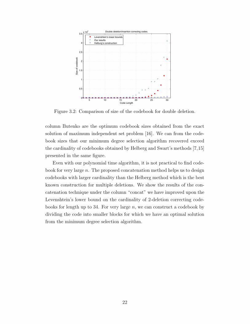
our construction improves upon Levenshtein lower bound for the 2-deletion

correcting codes for this range of n.

In Table 3.1, we compared maximum cardinalities obtained from Hel-

berg’s method [15] and our method. Note that for s = 1, Helberg’s code is

the same as Levenshtein’s code conjectured to be the optimal code for single

deletion correction [6]. For single deletion, VT code outperforms our heuris-

tic, but for larger number of deletions our codebook cardinalities are larger

than any previously known results, namely Helberg’s code. We have omited

s = 2 as they apperead in Table 3.2 already.

In Table 3.2, our results together with the best known cardinalities for

double deletion correcting codebooks are presented. The numbers under the

21

5 10 15 20 25 300

0.5

1

1.5

2

2.5

3

3.5 x 104

Code Length

Size

of c

odeb

ook

Double deletion/insertion correctng codes.

Levenshtein’s lower boundsOur resultsHelburg’s construction

Figure 3.2: Comparison of size of the codebook for double deletion.

column Butenko are the optimum codebook sizes obtained from the exact

solution of maximum independent set problem [16]. We can from the code-

book sizes that our minimum degree selection algorithm recovered exceed

the cardinality of codebooks obtained by Helberg and Swart’s methods [7,15]

presented in the same figure.

Even with our polynomial time algorithm, it is not practical to find code-

book for very large n. The proposed concatenation method helps us to design

codebooks with larger cardinality than the Helberg method which is the best

known construction for multiple deletions. We show the results of the con-

catenation technique under the column “concat” we have improved upon the

Levenshtein’s lower bound on the cardinality of 2-deletion correcting code-

books for length up to 34. For very large n, we can construct a codebook by

dividing the code into smaller blocks for which we have an optimal solution

from the minimum degree selection algorithm.

22

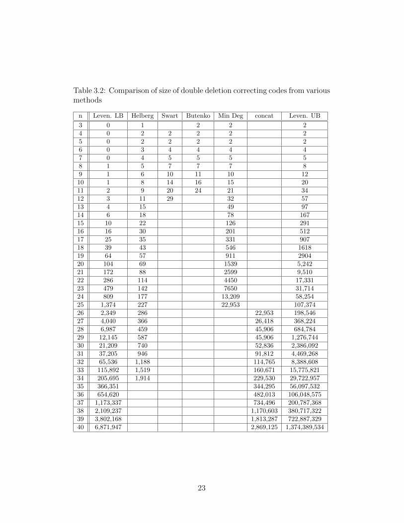
Table 3.2: Comparison of size of double deletion correcting codes from variousmethods

n Leven. LB Helberg Swart Butenko Min Deg concat Leven. UB

3 0 1 2 2 24 0 2 2 2 2 25 0 2 2 2 2 26 0 3 4 4 4 47 0 4 5 5 5 58 1 5 7 7 7 89 1 6 10 11 10 1210 1 8 14 16 15 2011 2 9 20 24 21 3412 3 11 29 32 5713 4 15 49 9714 6 18 78 16715 10 22 126 29116 16 30 201 51217 25 35 331 90718 39 43 546 161819 64 57 911 290420 104 69 1539 5,24221 172 88 2599 9,51022 286 114 4450 17,33123 479 142 7650 31,71424 809 177 13,209 58,25425 1,374 227 22,953 107,37426 2,349 286 22,953 198,54627 4,040 366 26,418 368,22428 6,987 459 45,906 684,78429 12,145 587 45,906 1,276,74430 21,209 740 52,836 2,386,09231 37,205 946 91,812 4,469,26832 65,536 1,188 114,765 8,388,60833 115,892 1,519 160,671 15,775,82134 205,695 1,914 229,530 29,722,95735 366,351 344,295 56,097,53236 654,620 482,013 106,048,57537 1,173,337 734,496 200,787,36838 2,109,237 1,170,603 380,717,32239 3,802,168 1,813,287 722,887,32940 6,871,947 2,869,125 1,374,389,534

23

CHAPTER 4

CONSTRUCTION OF CODES BASED ONCONCATENATION

4.1 Introduction

As mentioned in the previous chapter, the time complexity of the Min-Degree

selection algorithm becomes prohibitive as n grows. In this chapter, we are

going to use a concatenation method to generate larger codebooks. We will

prove a constructive lower bound on the size of the codebook and compare

our bound with the Levenshtein’s lower bound. The construction is based on

concatenation of codes with shorter blocks. It will construct an s-deletion and

insertion correcting code based on a given d s2e-deletion insertion correcting

code.

4.2 Concatenation and larger codebooks

In this section we will propose a construction method to form an s-deletion

correcting code from the concatenation of two sets of smaller codes. First

we will introduce a simple concatenation method to construct larger codes

from codes with smaller sizes. Then based on the concatenation idea, we will

introduce a method of construction that uses a code for smaller number of

deletions to construct a larger code that can correct more number of deletions.

4.2.1 A simple concatenation method for construction ofcodes with larger lengths

In this section we are going to use concatenation to generate larger codebooks.

Lemma 4.1. Let x, y ∈ F n2 and w = LCS(x, y). Length of w is less than

n− s if and only if dL(x, y) > 2s.

24

Proof. If length of w is less than n − s, then w ∈ Ds′(x) ∩ Ds′(y), where

s′ > s. Since w is LCS(x, y) for all s < s′: Ds(x) ∩ Ds(y) = ∅, then from

the proof of Lemma 3.1, dL(x, y) > 2s. Conversely, if dL(x, y) > 2s, then

Ds(x) ∩ Ds(y) = ∅. Then more than s bits should be deleted from both

sequences to get a common subsequence. Therefore, length of w is less than

s.

Theorem 4.2. Let C1 ∈ Cs,n1, C2 ∈ Cs,n2 be two sets of s-deletion correcting

code and let n = n1 +n2. Code C = C1×C2 is an s-deletion correcting code.

Proof. In order to prove this theorem, we present a decoding algorithm for

C1 × C2 as follows.

• Suppose that (n1+n2)-bit codeword c = c1c2 has been transmitted and

(n1 +n2− s′)-bit codeword r has been received, where c1 ∈ C1, c2 ∈ C2

and s′ ≤ s. Assume that in r, i deletions took place in c1 and s′ − ideletions took place in c2.

• To decode r, we need to decode remnant of c1 (denoted by r1) which

is the leftmost n1 − i bits of r and remnant of c2 by r2 which is the

rightmost n2 − (s′ − i) bits of r using C2 code.

• Since C1 can correct up to s deletions, we can remove another s′ − ibits from the right side of r1 (which will result in the leftmost n1 − s′

bits of r). This sequence of bits is what is left from c1 after s′ deletions,

so C1 decoder can construct c1 from it.

• Likewise, since C2 decoder can correct up to s deletions, we can remove

another i bits from the left side of r2 (which will result in the rightmost

n2 − s′ bits of c′). This sequence of bits is what is left from c2 after s′

deletions, so C2 decoder can construct c2 from it.

In the following, we will give an alternative proof for the theorem and we

will use it in the code construction.

Proof. Let’s think of the code C as a two segmented code where the first

segment is formed from codewords in C1 and the second segment is formed

from codewords in C2. Suppose x and y are two elements of C. Let x = x1x2

25

and y = y1y2, where x1, y1 ∈ C1 and x2, y2 ∈ C2. Suppose z = LCS(x, y).

We will show that the length of z should be less that n− s. If so, as a result

of Lemma 4.1, C is an s-deletion/insertion correcting code.

Suppose we have a common subsequence of x and y that has a length of

n − s. Assume s = s1 + s2 = s′1 + s′2 where s1 deletions occurred in x1, s2

in x2, s′1 in y1 and s′2 in y2. Note that s1, s2, s

′1 and s′2 are less than s. Let

n′1 = n1 − s′ where s′ = max{s1, s′1} ≤ s. Consider the first n′1 bits of z

as the substring z[1 . . . n′1] of z. Then z[1 . . . n′1] is a substring of a member

of Ds′(x1) and z[1 . . . n′1] ∈ Ds′(y1) therefore z[1 . . . n′1] ∈ Ds′(x1) ∩ Ds′(y1).

Thus for s′ ≤ s, Ds′(x1) ∩ Ds′(y1) 6= ∅. This is a contradiction because

x1, y1 ∈ C1 and C1 is an s-deletion/insertion correcting code. We could have

used the same argument for the second segment of the sequence. As a result,

for two sequences x and y in C, LCS(x, y) should have a length less than

n− s.

The following is immediate.

Corollary 4.3. For C1 ∈ Cs,n1, C2 ∈ Cs,n1, ..., Cm ∈ Cs,n1, C1×C2×· · ·×Cmis a Cs,∑m

i=1 nicode.

Proof. We prove this corollary using induction. The base of the induction

for m = 2 has been proved in the theorem above. For m > 2, we can divide

the concatenations into two parts. One containing C1 × · · · × Cm−1 and

the other containing Cm. Using the assumption of induction, we know that

C1 × · · · × Cm−1 is a Cs,∑m−1i=1 ni

. By applying the Theorem 4.2, we will have

Cs,∑m−1i=1 ni

× Cm = Cs,∑m

i=1 ni.

Using concatenation, we can easily generate deletion/insertion correcting

codebooks for higher dimensions. Note that decoding cost of these new

codebooks is equal to sum of decoding costs of the comprising parts.

4.2.2 A Special Case of Concatenation

Let us explain a simple special case. Consider C1 to be double-deletion-

correcting codebook of length 3 and C2 to be a larger double deletion cor-

recting codebook. The codewords in C1 are (000) and (111). Starting from

an initial codebook of length n, we can make a new codebook of length n+ 3

26

by concatenating three bits 000 or 111 with each elements of C2. This pro-

cess will take an initial codebook of length n of size m and expand it to a

codebook of length n+ 3 of size 2m.

From the above discussion, we can see that it is important to start con-

catenation of codes from larger blocks. Hence the superiority of our heuristic

algorithm is to create overall larger codebook starting from a large initial set

found from the maximal independent set algorithm.

The concatenation method proposed in this section relies on the avail-

ability of s-deletion correcting code of shorter length. In the next section we

will propose a new concatenation method that uses an s2-deletion correcting

code and gives an s-deletion correcting code.

4.2.3 Concatenation of codes using a buffer sequence

Definition 10 Suppose A ⊆ F n2 is a set of binary sequences partitioned

into p disjoint sets, i.e A =⋃pi=1Ai and ∀i 6= j, Ai ∩ Aj = ∅. Let B ⊆ Fm

2 is

another set of binary sequences that has a cardinality of p, |B| = p. Consider

an ordered set β = (β1, . . . , βp) which is a permutation of elements in the

set B, that each βi ∈ B. The extension of set A with the set β, denoted by

Ae(β), is defined as the following: Ae(β) =⋃pi=1Ai(βi) where Ai(βi) is the

Cartesian product of sequences in Ai with the sequence bi.

Ai(βi) = {X = x1x2|x1 ∈ Ai and x2 = βi} for βi ∈ B (4.1)

Note that |Ai(βi)| = |Ai| and |A| =⋃pi=1 |Ai| =

⋃pi=1 |Ai||βi| = |Ae(β)|.

For example for A = {000, 101} ∪ {100, 011} ∪ {010, 111} ∪ {001, 110} and

B = {00, 01, 10, 11}, the extended set A with the set β = (00, 01, 10, 11) is

demonstrated in the following.

A1(00) = {00000, 10100}

A2(01) = {10001, 01101}

A3(10) = {01010, 11110}

A4(11) = {00111, 11011}

(4.2)

27

Definition 11 An alignment is a sequence of deletion operations transform-

ing sequences x and y into a common subsequence of these two sequences.

The minimum number of deletion operations is used when we are aligning x

and y to LCS(x, y) sub-sequence. We will show that the alignment is not

possible for less than or equal to s number of deletions.

Theorem 4.4. Consider the sets A1, A2, . . . , Ap ⊂ F n12 and B1, B2, . . . , Bq ⊂

F n22 be such that

∀x1 ∈ Ai, y1 ∈ Aj :

{dL(x1, y1) > 2s if i = j

dL(x1, y1) > s if i 6= j

∀x2 ∈ Bi, y2 ∈ Bj :

{dL(x2, y2) > 2s if i = j

dL(x2, y2) > s if i 6= j

The sets are such that |A1| ≥ |A2| ≥ · · · ≥ |Ap| and |B1| ≥ · · · ≥ |Bq|. Let

m = min{p, q} and β ⊆ Cs,n3,where n3 is chosen such that |β| ≥ m. A code

C constructed such that C =⋃mi=1Ci =

⋃mi=1Ai(βi)× Bi can correct up to s

number of deletions, where n = n1 + n2 + n3.

Proof. Code C can be seen as a two segmented code joined with a buffer

sequence. Let’s call the first segment A and the second segment B. We are

concatenating each of Ai sets with a fixed sequence βi and then concatenating

it with the second code Bi. The first segment of the code is that part the

originated from A set and the B segment is the part from B set and the buffer

sequence is from the β set. Within segment A, dL(A) > s, hence segment

A is an b s2c- deletion correcting codes. This means that for any x1, y1 ∈ A

and s′ ≤ b s2c, Ds′(x1) ∩Ds′(y1) = ∅. So, none of the subsequences of length

n1 − b s2c are equal. This property also holds for segment B.

Let x = x1βix2 and y = y1βjy2, where x1 ∈ Ai, y1 ∈ Bi and x2 ∈ Aj, y2 ∈Bj and βi, βj ∈ β. Two cases will arise:

Case 1: i = j

In this case, x1, y1 ∈ Ai and x2, y2 ∈ Bi where dL(Ai) > 2s and dL(Bi) >

2s. Hence, Ai is a Cs,n1 code and Bi is also a Cs,n2 code. Ci is formed from

concatenation of a Cs,n1 code and a Cs,n2 code and a buffer sequence βi. As

a result of Lemma 4.8, it is a Cs,n code.

Case 2: i 6= j

In this case, x1 6= y1 and x2 6= y2. Let’s assume we sent x and y, and s

28

deletions occurred. We will show that the subsequences cannot be similar.

The number of deletions in each segment can take values from 0 to s. In

either of segments dL(xk, yk) > s for k = 1, 2, then within each segments b s2c

deletions can be corrected.

We will study different cases where deletions can happen and then we will

use Lemma 4.1 to show that C is an s-deletion/insertion correcting code. We

will show that there is no way of getting a common subsequence of length at

least n− s from codewords in code C after deletions. Let n− s be the length

of the received code.

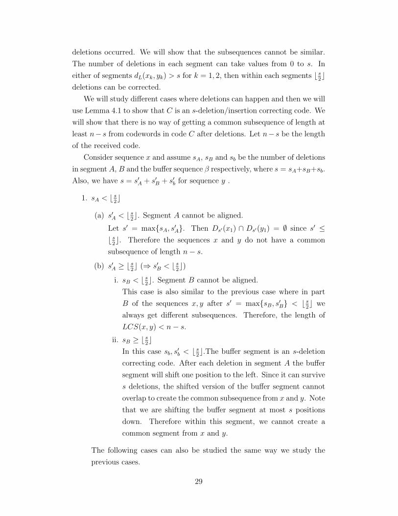
Consider sequence x and assume sA, sB and sb be the number of deletions

in segmentA, B and the buffer sequence β respectively, where s = sA+sB+sb.

Also, we have s = s′A + s′B + s′b for sequence y .

1. sA < b s2c

(a) s′A < b s2c. Segment A cannot be aligned.

Let s′ = max{sA, s′A}. Then Ds′(x1) ∩ Ds′(y1) = ∅ since s′ ≤b s2c. Therefore the sequences x and y do not have a common

subsequence of length n− s.

(b) s′A ≥ b s2c (⇒ s′B < b s2c)

i. sB < b s2c. Segment B cannot be aligned.

This case is also similar to the previous case where in part

B of the sequences x, y after s′ = max{sB, s′B} < b s2c we

always get different subsequences. Therefore, the length of

LCS(x, y) < n− s.ii. sB ≥ b s2c

In this case sb, s′b < b s2c.The buffer segment is an s-deletion

correcting code. After each deletion in segment A the buffer

segment will shift one position to the left. Since it can survive

s deletions, the shifted version of the buffer segment cannot

overlap to create the common subsequence from x and y. Note

that we are shifting the buffer segment at most s positions

down. Therefore within this segment, we cannot create a

common segment from x and y.

The following cases can also be studied the same way we study the

previous cases.

29

2. sA ≥ b s2c (⇒ sB < b s2c)

(a) s′A < b s2c

i. s′B < b s2c. Segment B cannot be aligned.

ii. s′B ≥ b s2c. The buffer segment cannot be aligned.

(b) s′A ≥ b s2c (⇒ s′B < b s2c). Segment B cannot be aligned.

Let A =⋃pi=1Ai. The set A is an independent set in Lb s

2c,n and each

Ai sets are also an independent set in Ls,n. Let b ⊆ Cs,m, for m such that

|Cs,m| ≥ p, and let bi be elements of b. We will prove that m ≤ O(log n).

Form a code C of length n′ = 2n + m from the concatenation of Ai, bi

and Ai as the following:

Lemma 4.5. Supposed a code C formed as the following:

C =

p⋃i=1

Ai(bi)× Ai.

Then the cardinality of the code can be bounded by |A|2

pfrom below.

Proof. First, we will obtain an inequality from Cauchy-Schwarz inequality.

Then a second inequality will be obtained from the union bound as follows.

|C| =p∑i=1

|Ai|2 ≥(∑p

i=1 |Ai|)2

p≥ 1

p|p⋃i=1

Ai|2 =|A|2

p(4.3)

To get the largest cardinality for code C, we should use the largest possible

set as A, then partition it into smallest possible number of sets which is p. In

the next section, we will see how these optimal values can be calculated.

The concatenation with buffer sequence can be used more efficiently.

Since we only used the distance characteristic of partitions and we didn’t

used the indices, there is a better way of concatenating the segments in or-

der to get codes of larger sizes. In the next section, we will introduce this

optimal concatenation.

30

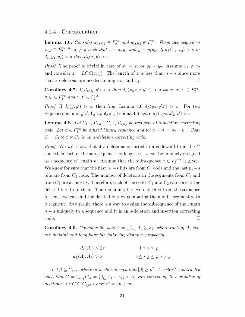
4.2.4 Concatenation

Lemma 4.6. Consider x1, x2 ∈ F n12 and y1, y2 ∈ F n2

2 . Form two sequences

x, y ∈ F n1+n22 , x 6= y such that x = x1y1 and y = y1y2. If dL(x1, x2) > s or

dL(y1, y2) > s then dL(x, y) > s.

Proof. The proof is trivial in case of x1 = x2 or y1 = y2. Assume x1 6= x2

and consider z = LCS(x, y). The length of z is less than n − s since more

than s-deletions are needed to align x1 and x2.

Corollary 4.7. If dL(y, y′) > s then dL(xyz, x′y′z′) > s where x, x′ ∈ F n12 ,

y, y′ ∈ F n22 and z, z′ ∈ F n3

2 .

Proof. If dL(y, y′) > s, then from Lemma 4.6 dL(yz, y′z′) > s. For two

sequences yz and y′z′, by applying Lemma 4.6 again dL(xyz, x′y′z′) > s.

Lemma 4.8. Let C1 ∈ Cs,n1, C2 ∈ Cs,n2 be two sets of s-deletion correcting

code. Let β ∈ F n32 be a fixed binary sequence and let n = n1 + n2 + n3. Code

C = C1 × β × C2 is an s-deletion correcting code.

Proof. We will show that if s deletions occurred in a codeword from the C

code then each of the sub-sequences of length n− s can be uniquely assigned

to a sequence of length n. Assume that the subsequence z ∈ F n−s2 is given.

We know for sure that the first n1−s bits are from C1 code and the last n2−sbits are from C2 code. The number of deletions in the segments from C1 and

from C2 are at most s. Therefore, each of the codes C1 and C2 can correct the

deleted bits from them. The remaining bits were deleted from the sequence

β, hence we can find the deleted bits by comparing the middle segment with

β segment. As a result, there is a way to assign the subsequence of the length

n− s uniquely to a sequence and it is an s-deletion and insertion correcting

code.

Corollary 4.9. Consider the sets A =⋃pi=1Ai ⊆ F n

2 where each of Ai sets

are disjoint and they have the following distance propoerty:

dL(Ai) > 2s 1 ≤ i ≤ p

dL(Ai, Aj) > s 1 ≤ i, j ≤ p, i 6= j.

Let β ⊆ Cs,m, where m is chosen such that |β| ≥ p2. A code C constructed

such that C =⋃i,j Cij =

⋃i,j Ai × βij × Aj can correct up to s number of

deletions, i.e C ⊆ Cs,n′,where n′ = 2n+m.

31

Proof. Let x = x1βijx2 and y = y1βkly2, where x1 ∈ Ai, x2 ∈ Aj and y1 ∈Ak, y2 ∈ Al and βij, βkl ∈ β. Two cases will arise:

Case 1: βij = βkl

In this case, x1, y1 ∈ Ai and x2, y2 ∈ Aj where dL(Ai) > 2s and dL(Aj) >

2s. Hence, each of the Ai and Aj is a Cs,n code. Cij is formed from con-

catenation of a Cs,n code, a buffer sequence βij and another Cs,n code. As a

result of Lemma 4.8, it is a Cs,n code.

Case 2: βij 6= βkl The set β is an s deletion/insertion correcting code.

Therefore, if βij 6= βkl, dL(βij, βkl) > 2s. From Corollary 4.7, for any x and

y constructed βij, βkl as the middle segment, dL(x, y) > 2s.

Algorithm 2 will select such disjoint sets. It starts with the graph Ls,n,

and finds an independent set in this graph and assign it to the first Ai set.

Then it forms a new graph by removing all the nodes in the independent

set and their neighbors within the Levenshtein distance of s of the selected

nodes. It repeats the same procedure for the new graph.

Algorithm 2. Selection of s-distance disjoint setsInput: Graph G(V,E) and MIS(G) as a subroutine for

maximal independent set problem:

1. Initialize G0 = G;2. Output A0 = MIS(G0);3. i = 0;4. while (|Gi| 6= 0) {5. Gi+1 = Gi/ {Ai ∪ {

⋃si=1Ni(Ai)}};

6. Ai+1 = MIS(Gi+1);7. i = i+ 1;8. Output Ai; }

The partitioning of A and B sets is important in the proposed construc-

tion. In the next section, we will see how the disjoint sets Ai can be generated.

We will relate this problem to the graph coloring problem.

32

4.3 Partitioning and vertex coloring of the graph

Lemma 4.10. Let A be an independent set in Ld s2e,n graph. The minimum

coloring of the Ls,n(A) graph is a partitioning of A set into s-distance disjoint

sets with minimum number of sets.

Proof. From equation (4.3), and the fact that the set A is an independent set

in Ld s2e,n, the set A should be chosen such that it is the maximum independent

set in Ld s2e,n. Furthermore, the number of parts we get in the partitioning of

A also should be the smallest possibe number.

Consider the graphs Ld s2e,n, Ls,n and the set A as the set of their vertices.

Since Ls,n has the same vertex set and also contains all edges of Ld s2e,n the

graph Ld s2e,n is in Ls,n. For nodes u, v ∈ A, dL(u, v) > s. Consider the graph

Ls,n(A) which is the subgraph of Ls,n induces by the set A. Choose the A set

such that it is an independent set in Ld s2e,n. A coloring for the graph Ls,n(A)

will give the required partitioning of A. In this partitioning, each of the Ai

sets is a color class in Ls,n(A). Therefore they are independent sets in Ls,n

and can satisfy the distance properties.

In the next section, we will calculate bounds on the size of the code

generated from the concatenation and we will compare the bounds by the

asymptotic bounds of Levenshtein [3].

4.4 Bounds on the size of the code

Levenshtein [3] provide asymptotic upper and lower bounds on the size of

codebook with s-deletions/insertions. For fixed s, as n→∞,

2s(s!)22n

n2s≤ |Cs,n| ≤

s!2n

ns

Example For s = 2, this formula will reduce to

2n+4

n4≤ |C| ≤ 2n+1

n2.

Leveneshtein also proved that any codebook that can correct s-deletions (or

insertion), can correct s number of deletions and insertions [3]. The concate-

nation method discussed in the previous section can be used to construct

33

multiple deletion/insertion correcting codes in a recursive way. Given an

d s2e-deletion/insertion correcting code of length n, one can construct an s-

deletion/insertion code of length 2n+ α log n.

Suppose A1, A2, . . . , Ap are p disjoint sets of sequences in F n2 . The Ai sets

were selected such that

∀x, y ∈ Ai : dL(x, y) > 2s (4.4)

∀x ∈ Ai, y ∈ Aj, i 6= j : dL(x, y) > s (4.5)

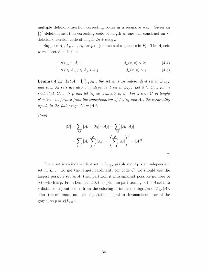
Lemma 4.11. Let A =⋃pi=1Ai , the set A is an independent set in Ld s

2e,n

and each Ai sets are also an independent set in Ls,n. Let β ⊆ Cs,m for m

such that |Cs,m| ≥ p and let βij be elements of β. For a code C of length

n′ = 2n+m formed from the concatenation of Ai, βij and Aj, the cardinality

equals to the following: |C| = |A|2.

Proof.

|C| =∑i,j

|Ai| · |βij| · |Aj| =∑i,j

|Ai||Aj|

=

p∑i=1

|Ai|p∑j=1

|Aj| =

(p∑i=1

|Ai|

)2

= |A|2

The A set is an independent set in Ld s2e,n graph and A1 is an independent

set in Ls,n. To get the largest cardinality for code C, we should use the

largest possible set as A, then partition it into smallest possible number of

sets which is p. From Lemma 4.10, the optimum partitioning of the A set into

s-distance disjoint sets is from the coloring of induced subgraph of Ls,n(A).

Thus the minimum number of partitions equal to chromatic number of the

graph, so p = χ(Ls,n).

34

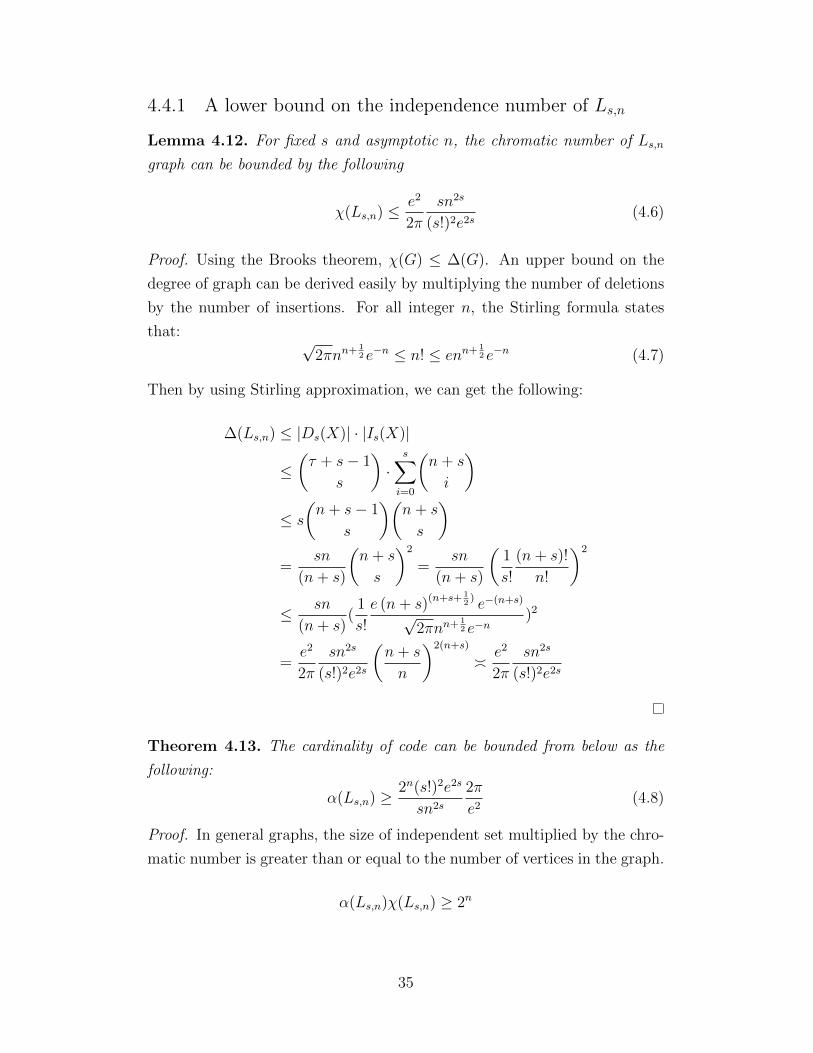
4.4.1 A lower bound on the independence number of Ls,n

Lemma 4.12. For fixed s and asymptotic n, the chromatic number of Ls,n

graph can be bounded by the following

χ(Ls,n) ≤ e2

2π

sn2s

(s!)2e2s(4.6)

Proof. Using the Brooks theorem, χ(G) ≤ ∆(G). An upper bound on the

degree of graph can be derived easily by multiplying the number of deletions

by the number of insertions. For all integer n, the Stirling formula states

that: √2πnn+

12 e−n ≤ n! ≤ enn+

12 e−n (4.7)

Then by using Stirling approximation, we can get the following:

∆(Ls,n) ≤ |Ds(X)| · |Is(X)|

≤(τ + s− 1

s

)·

s∑i=0

(n+ s

i

)≤ s

(n+ s− 1

s

)(n+ s

s

)=

sn

(n+ s)

(n+ s

s

)2

=sn

(n+ s)

(1

s!

(n+ s)!

n!

)2

≤ sn

(n+ s)(

1

s!

e (n+ s)(n+s+12) e−(n+s)

√2πnn+

12 e−n

)2

=e2

2π

sn2s

(s!)2e2s

(n+ s

n

)2(n+s)

� e2

2π

sn2s

(s!)2e2s

Theorem 4.13. The cardinality of code can be bounded from below as the

following:

α(Ls,n) ≥ 2n(s!)2e2s

sn2s

2π

e2(4.8)

Proof. In general graphs, the size of independent set multiplied by the chro-

matic number is greater than or equal to the number of vertices in the graph.

α(Ls,n)χ(Ls,n) ≥ 2n

35

Lemma 4.12 gives the chromatic number. Therefore, we have the following:

α(Ls,n) ≥ 2n

χ(Ls,n)≥ 2n

e2

2πsn2s

(s!)2e2s

=2n(s!)2e2s

sn2s

2π

e2

Lemma 4.14. For all fixed s, the lower bound obtained from the coloring is

greater than the Levenshtein’s lower bound.

Proof. The ratio between the bound from coloring and the Levenshtein’s

lower bound is always greater than one:

2n(s!)2e2s

sn2s2πe2

2s(s!)22n

n2s

=2π

se2

(e2

2

)s≥ 1 (4.9)

Example For the case of s = 2, the lower bound on the size of the codebook

is 4πe22n

n4 ≈ 232n

n4 , which is greater than the Leveneshtein’s lower bound of 2n+4

n4 .

In the following we are going to see how a single deletion correcting code

can be used to construct a double deletion code.

4.4.2 Construction of single deletion correcting code fromconcatenation

Suppose a set A =⋃pi=1Ai, A ⊆ F n

2 is given such that ∀1 ≤ i ≤ p : dL(Ai) >

2 and ∀i 6= j : Ai ∩ Ai = ∅, dL(Ai, Aj) > 1. Let β is also a single deletion

correcting code of length m with cardinality at least p. We will prove that

m ≤ O(log n). For a code C =⋃pi=1Ai(βi) ∗Ai, from equation (4.3) the size

can be bounded as |C| =∑p

i=1 |Ai|2 ≥|A|2p

.

Sloane [6] proved that for fixed n, V T0(n) has the largest cardinality

between all VT-codes, for any 0 ≤ a ≤ n. A lower bound on the size V T0(n)

can be obtained from the following:

|V T0(n)| ≥ 2n

n+ 1(4.10)

For sequences with the same length the Levenshtein distance is always an

even number since the number of deletions and insertions should be equal.

36

Suppose u, v ∈ F n2 , u 6= v, then dL(u, v) ≥ 2. So the condition dL(Ai, Aj) > 1

is automatically satisfied. If we take the set A to be F n2 , then partition the

induces graph on A vertices is L1,s graph and the Ai sets are color classes

in the graph. A possible coloring for the binary sequences of length n are

the coloring from the VT-codes. In this coloring the codes are divided into

n + 1 groups, thus p = n + 1. The set be should be chosen such that it is

a one deletion correcting code. Choosing set β from V T0(m) suggest that

|V T0(m)| ≥ 2m

m+1> p = n + 1. By taking m = 2 log n, we can satisfy the

previous equation. The bounds of Levenshtein for one deletion correcting

codes2n+1

n2≤ |C1,n| ≤

2n

n.

A code C of length 2n+m can be constructed with cardinality:

|C| =p∑i=1

|Ai|2 = |A|2 = (2n)2 (4.11)

The upper bound of Levenshtein for a code with equal length says that the

cardinality of the optimal code is less than 22n+m

2n+m. To see how far we are from

the V T -code, we will calculate the ratio of the sizes.

Lemma 4.15. For a code C of length n′ = 2n + m from the concatenation

of Ai, βi and Ai the cardinality is bounded by:

O(n · log n) ≤ |C1,n′||C|

≤ O(n2)

Proof. The bounds can be calculated from the following:

From the results of concatenation we have |C| ≤ |C1,m| · |A1|2, and since

|A1| ≤ |V T0(n)| ≤ 2n

nand m = 2 log n

|C1,n′||C|

≥22n+m

2n+m+1

2m

m+1· 22nn2

=(m+ 1) · n2

(2n+m+ 1)

=(2 log n+ 1)n2

(2n+ 2 log n+ 1)= O(n · log n)

|C1,n′ ||C|

≤22n+m

2n+m

22n

n+1

=(n+ 1)2m

2n+m=

(n+ 1)n2

2n+ 2 log n= O(n2)

37

Definition 12 The rate of a block code C of length n is defined as the

ratio of the cardinality of C divided by n, R = |C|n

.

Theorem 4.16. For single deletion, the rate of the code formed from the

concatenation asymptotically achieves the rate of optimum code.

Proof. Suppose C1,n′ is the optimum code and C is the code formed from the

concatenation of two codes of length n and a buffer of length m = 2 log n.

From Lemma 4.15, we can see the following:

log (O(n · log n))

n≤

log(|C1,n′ ||C|

)n

≤ log (O(n2))

n

As n goes to infinity, from the sandwich theorem, limn→∞Ropt −R = 0.

4.4.3 Construction of 2-deletion correcting codes fromcoloring of VT codes

In this section, we will study the recursive construction of double deletion

correcting codes, C2,n code from s = 1 deletion correcting codes. Fortunately,

for s = 1, there is an algebraic construction for these codes. The VT-code,

introduced by Levenshtein is conjectured to be the optimal code, which is

the maximum independent set in L1,n graph [6].

Suppose we are interested in finding double deletion correcting codes.

The recursive construction introduced in this chapter is such that the set A

is one deletion correcting code. If we take V Ta(n) as this A set, and find a

coloring for the graph induced by these vertices, we would be able to find

the Ai partitions. As proved in [6], V T0(n) has the largest size between all

V T -codes, we would take this code as the A set.

Lemma 4.17. The size of the 2-deletion correcting code obtained by the

coloring of the induced subgraph of the L2,n graph on V T0(n) is greater than4πe22n

n4(n+1).

Proof. In the previous section we discussed about the partitioning and its

relation to the chromatic number of a graph. We saw that the number of parts

38

is equal to the chromatic number of the induced subgraph of L2,n. Moreover,

the chromatic number of the induced subgraph of a graph is not more than

the chromatic number of the original graph. Therefore, χ (L2,n (V T0(n))) ≤χ (L2,n) ≤ e2

2π2n2∗2

(2!)2e2∗2= n4

4πe2. Hence, we can bound the size of the largest

color class by dividing the size of the subgraph by chromatic number. The

size of V T0(n) code is greater than 2n

n+1[6]. Therefore, we will get the 4πe22n

n4(n+1)

bound.

4.5 Conclusion

In this chapter, we studied a concatenation method for the construction of

larger deletion and insertion correcting codes based on smaller codes. Specif-

ically we showed how our construction works for special cases such as single

and double deletion correcting codes. Moreover, we proved a new lower

bound on the size of the general codes based on a coloring argument. The

new lower bound on the size of s-deletion correcting code is larger than the

lower bound of Levenshtein [3].

39

CHAPTER 5

CONCLUSION

We introduced a new method to search for multiple insertion/deletion error

correcting codes. Our approach works for any number of deletion and inser-

tions s and any code length n. Our approach first recovers a codebook based

on a heuristic algorithm which finds the maximal independent set in an ap-

propriately defined graph and then uses an optimal concatenation technique

to find codebooks that accommodate a larger code length n.

The heuristic algorithm does far better than the optimal concatenation

approach if it could be applied to larger n. However, the complexity of the

algorithm renders this method infeasible for n beyond 25 (although this is

already an improvement over the existing work). Hence, for larger n, concate-

nation technique is employed. It is obvious that the concatenation principle

is not particularly efficient for constructing codebooks of larger length from

codebooks of smaller length. However, given lack of alternatives, by starting

from a larger initial codebook found through the heuristic algorithm, we con-

struct codebooks of much larger cardinalities compared to previous works.

We surmise that the superior performance of the heuristic algorithm is in

fact the result of special structure of the graph. In future, we plan to use

this special structure to come up with better constructions for deletion and

insertion codes. It will be interesting to see if the structure of the graph may

also be utilized to find efficient decoding algorithms.

In future, we can use this special structure to come up with better con-

structions for deletion and insertion codes. The concatenation method gives

some idea for designing an exact algorithm that uses the special structure of

these graphs. We hope that the structure of the graph may also be utilized

to find efficient decoding algorithms.

40

APPENDIX A

COMPLEXITY OF THE GREEDYALGORITHM

A.1 Time complexity and performance of the greedy

algorithm

Using Min-Heap data structure [24] to store the vertices indexed by the

values of d(v), we can easily find the vertex with minimum degree in O(1).

Initializing the heap time costs O(|V |) and we can remove the elements or

change the index values (d(v)), and then update the Heap in O(lg(|V |)).The algorithm starts with a continuous range of numbers from 0 to 2n − 1

representing vertices in V , so we can use an index array to locate the nodes

in Min-Heap in O(1).

Considering the fact that each node is removed exactly once from the

heap (O(|V |. lg(|V |))) and the total number of updates on the values of d(v)

cannot exceed the number of edges in the graph (O(|E|. lg(|V |))), we can

compute the time complexity of Min-Degree Selection algorithm (since each

node has at least one neighbor, then we have |V | ∈ O(|E|)):

O(|V |) +O(|V |. lg(|V |)) +O(|E|. lg(|V |))

= O(|E|. lg(|V |)) = O(|E|.n). (A.1)

Although this algorithm is polynomial regarding the size of the graph

(|V |), we should keep mind that linear increment of n leads to exponential

growth of the size of the graph (V and E). Hence, this algorithm is non-

polynomial regarding the length of the codes, which is the real parameter of

the problem. As a result, using this algorithm for large values of n is not

practical. However, it is worth mentioning that this approach executed on

a normal PC, can provide us with codebooks of length 20 in less than one

hour and codebooks of length 25 in less than one day.

41

APPENDIX B

DEGREE OF ONE DELETION GRAPHS

B.1 Definitions and background

Let G = (V,E) be an undirected graph where each vertex v ∈ V is a binary

sequence of length n. There are |F n2 | = 2n vertices in this graph. An edge is

drawn between two vertices u and v if any of the subsequences they produce

after any s number of deletions are the same. We are interested in finding a

formula for the degree of this graph. For s = 1 we proved the exact formula

for the degree of each vertices by using the results Levenshtein proved in [3]

and [18].

For a binary sequence X of length n, let Ds(X) and Is(X) denote the

set of all binary sub-sequences and super-sequences obtained from X by s

number of deletions and insertions respectively. Let τ be the number of runs

in the sequence X. Levenshtein proved formulas for the maximum number

of sub and super sequence, any two binary sequences of length n can produce

after s-deletions and insertions [3], [18].

For all binary sequences of length n, let N−(n, s) and N+(n, s) denote the

maximum size of the common subsequences and super sequences of length

n− s and n+ s respectively.

N−(n, s) = maxx,y∈Fn

2

|Ds(x) ∩Ds(y)| = 2s−1∑i=0

(n− s− 1

i

)(B.1)

N+(n, s) = maxx,y∈Fn

2

|Is(x) ∩ Is(y)| = 2s−1∑i=0

(n+ s− 1

i

)(B.2)

In the case where s = 1 the above formulas will be reduced to the follow-

ing: D(X) = τ , I(X) = n+ 2 and N+(n, 1) = N−(n, 1) = 2.

The Levenshtein distance dL(x, y) between two sequence x and y is defined

42

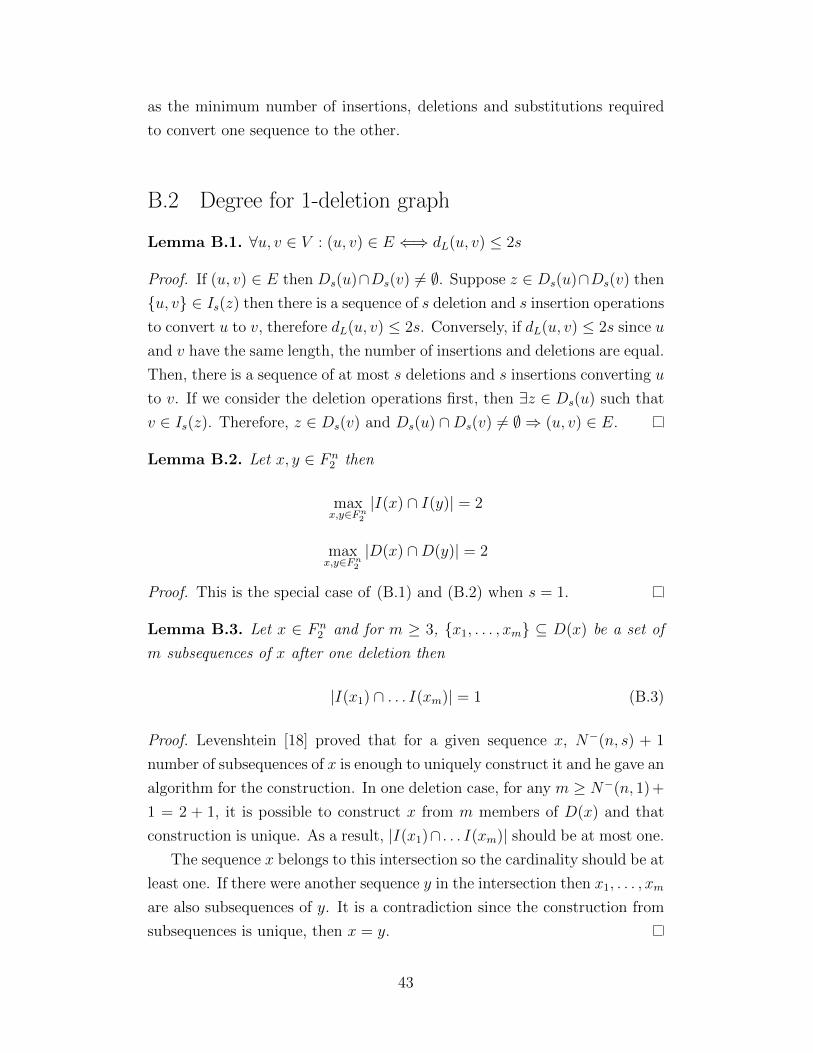
as the minimum number of insertions, deletions and substitutions required

to convert one sequence to the other.

B.2 Degree for 1-deletion graph

Lemma B.1. ∀u, v ∈ V : (u, v) ∈ E ⇐⇒ dL(u, v) ≤ 2s

Proof. If (u, v) ∈ E then Ds(u)∩Ds(v) 6= ∅. Suppose z ∈ Ds(u)∩Ds(v) then

{u, v} ∈ Is(z) then there is a sequence of s deletion and s insertion operations

to convert u to v, therefore dL(u, v) ≤ 2s. Conversely, if dL(u, v) ≤ 2s since u

and v have the same length, the number of insertions and deletions are equal.

Then, there is a sequence of at most s deletions and s insertions converting u

to v. If we consider the deletion operations first, then ∃z ∈ Ds(u) such that

v ∈ Is(z). Therefore, z ∈ Ds(v) and Ds(u) ∩Ds(v) 6= ∅ ⇒ (u, v) ∈ E.

Lemma B.2. Let x, y ∈ F n2 then

maxx,y∈Fn

2

|I(x) ∩ I(y)| = 2

maxx,y∈Fn

2

|D(x) ∩D(y)| = 2

Proof. This is the special case of (B.1) and (B.2) when s = 1.

Lemma B.3. Let x ∈ F n2 and for m ≥ 3, {x1, . . . , xm} ⊆ D(x) be a set of

m subsequences of x after one deletion then

|I(x1) ∩ . . . I(xm)| = 1 (B.3)

Proof. Levenshtein [18] proved that for a given sequence x, N−(n, s) + 1

number of subsequences of x is enough to uniquely construct it and he gave an

algorithm for the construction. In one deletion case, for any m ≥ N−(n, 1)+

1 = 2 + 1, it is possible to construct x from m members of D(x) and that

construction is unique. As a result, |I(x1)∩ . . . I(xm)| should be at most one.

The sequence x belongs to this intersection so the cardinality should be at

least one. If there were another sequence y in the intersection then x1, . . . , xm

are also subsequences of y. It is a contradiction since the construction from

subsequences is unique, then x = y.

43

Suppose x is a sequence of length n with τ number of runs. Let D(x) be

the set of all subsequences of x after one deletion. Since sequence x has τ

number of runs, |D(x)| = τ and each subsequence is obtained from deletion

of one bit from a given run. If a subsequence was obtained from deletion of

a bit from i’th run, we call that subsequence xi. Therefore we can right the

set D(x) as the following: D(x) = {x1, . . . , xτ}. Define Ai = I(xi) the set of

all supersequences of xi after one insertion where xi is a subsequence of x.

Lemma B.4. Let N(x) denotes the set of all vertices in the neighborhood of

x. Then we have the following:

N(x) ∪ {x} = A1 ∪ · · · ∪ Aτ

Proof. The sequences in the neighborhood of x have Levenshtein distance of

2 to it. The set A1 ∪ · · · ∪ Aτ has all possible sequences obtained from x

by one deletion and one insertion. So, excluding the sequence itself, all the

members of this set are within distance 2 as a result of lemma B.1, they are

in neighborhood of x.

Suppose x ∈ F n2 and is written in the run-length representation. For

1 ≤ i ≤ n− 2 define pi as the number of i consecutive single runs excluding

the extreme runs. In other words, in the run length representation, p1 is

the number of −1− patterns, p2 is the number of −11− patterns, p3 is the

number of −111− patterns and so on.

For example, if x = 01011010, the run length representation is x =

1112111. The values of pi can be calculated as the following. We can easily

see p1 = 4 because it is the number of middle runs with length 1, p2 = 2

since we have two of −11− patterns in the sequence as depicted by an over

line 1112111 and p3 = p4 = ... = p6 = 0 since there are no more than 2

consecutive one-runs in the sequence.

Lemma B.5. Let x ∈ F n2 , xi ∈ D(x), Ai = I(xi) and [τ ] = {1, 2, . . . , τ}

then ∑i,j

|Ai ∩ Aj| =(τ

2

)+ τ − 1 +

n−2∑i=1

pi

Proof. For all i, x ∈ Ai then |Ai ∩ Aj| ≥ 1 and from lemma B.2,

44

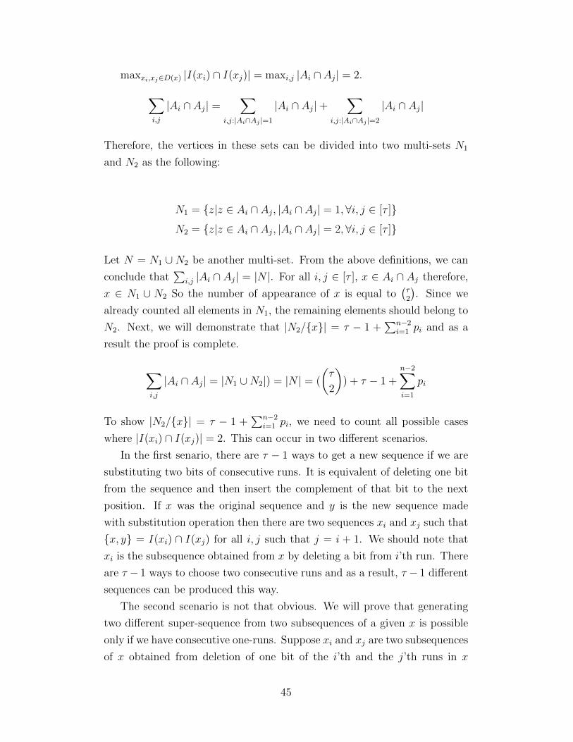
maxxi,xj∈D(x) |I(xi) ∩ I(xj)| = maxi,j |Ai ∩ Aj| = 2.∑i,j

|Ai ∩ Aj| =∑

i,j:|Ai∩Aj |=1

|Ai ∩ Aj|+∑

i,j:|Ai∩Aj |=2

|Ai ∩ Aj|

Therefore, the vertices in these sets can be divided into two multi-sets N1

and N2 as the following:

N1 = {z|z ∈ Ai ∩ Aj, |Ai ∩ Aj| = 1,∀i, j ∈ [τ ]}

N2 = {z|z ∈ Ai ∩ Aj, |Ai ∩ Aj| = 2,∀i, j ∈ [τ ]}

Let N = N1 ∪ N2 be another multi-set. From the above definitions, we can

conclude that∑

i,j |Ai ∩ Aj| = |N |. For all i, j ∈ [τ ], x ∈ Ai ∩ Aj therefore,

x ∈ N1 ∪ N2 So the number of appearance of x is equal to(τ2

). Since we

already counted all elements in N1, the remaining elements should belong to

N2. Next, we will demonstrate that |N2/{x}| = τ − 1 +∑n−2

i=1 pi and as a

result the proof is complete.

∑i,j

|Ai ∩ Aj| = |N1 ∪N2|) = |N | = (

(τ

2

)) + τ − 1 +

n−2∑i=1

pi

To show |N2/{x}| = τ − 1 +∑n−2

i=1 pi, we need to count all possible cases

where |I(xi) ∩ I(xj)| = 2. This can occur in two different scenarios.

In the first senario, there are τ − 1 ways to get a new sequence if we are

substituting two bits of consecutive runs. It is equivalent of deleting one bit

from the sequence and then insert the complement of that bit to the next

position. If x was the original sequence and y is the new sequence made

with substitution operation then there are two sequences xi and xj such that

{x, y} = I(xi) ∩ I(xj) for all i, j such that j = i + 1. We should note that

xi is the subsequence obtained from x by deleting a bit from i’th run. There

are τ − 1 ways to choose two consecutive runs and as a result, τ − 1 different

sequences can be produced this way.

The second scenario is not that obvious. We will prove that generating

two different super-sequence from two subsequences of a given x is possible

only if we have consecutive one-runs. Suppose xi and xj are two subsequences

of x obtained from deletion of one bit of the i’th and the j’th runs in x

45

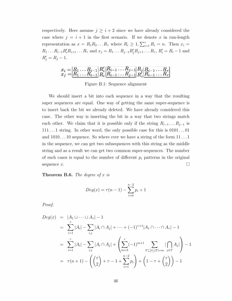
respectively. Here assume j ≥ i + 2 since we have already considered the

case where j = i + 1 in the first scenario. If we denote x in run-length

representation as x = R1R2 . . . Rτ where Ri ≥ 1,∑τ

i=1Ri = n. Then xi =

R1 . . . Ri−1R′iRi+1 . . . Rτ and xj = R1 . . . Rj−1R

′jRj+1 . . . Rτ , R

′i = Ri− 1 and

R′j = Rj − 1.

Figure B.1: Sequence alignment

We should insert a bit into each sequence in a way that the resulting

super sequences are equal. One way of getting the same super-sequence is

to insert back the bit we already deleted. We have already considered this

case. The other way is inserting the bit in a way that two strings match

each other. We claim that it is possible only if the string Ri−1 . . . Rj−1 is

111 . . . 1 string. In other word, the only possible case for this is 0101 . . . 01

and 1010 . . . 10 sequence. So where ever we have a string of the form 11 . . . 1

in the sequence, we can get two subsequences with this string as the middle

string and as a result we can get two common super-sequences. The number

of such cases is equal to the number of different pi patterns in the original

sequence x.

Theorem B.6. The degree of x is

Deg(x) = τ(n− 1)−n−2∑i=0

pi + 1

Proof.

Deg(x) = |A1 ∪ · · · ∪ Aτ | − 1

=τ∑i=1

|Ai| −∑i,j

|Ai ∩ Aj|+ · · ·+ (−1)τ+1|A1 ∩ · · · ∩ Aτ | − 1

=τ∑i=1

|Ai| −∑i,j

|Ai ∩ Aj|+

τ∑m=3

(−1)m+1∑

T⊆[τ ],|T |=m

|⋂j∈T

Aj|

− 1

= τ(n+ 1)−

((τ

2

)+ τ − 1 +

n−2∑i=1

pi

)+

(1− τ +

(τ

2

))− 1

46

= τ(n− 1)−n−2∑i=0

pi + 1

From (2.6) we have |Ai| = |I(xi)| = n+ 1. In lemma B.3 we proved that

for all m ≥ 3 sets of subsequences, |A1∩· · ·∩Am| = 1. Let [τ ] = {1, 2, . . . , τ}

∑T ⊆ [τ ]

|T | = m

|⋂j∈T

Aj| =∑

T ⊆ [τ ]

|T | = m

1 =

(τ

m

)

τ∑m=3

(−1)m+1∑

T⊆[τ ],|T |=m

|⋂j∈T

Aj| = −τ∑

m=3

(−1)m∑

T⊆[τ ],|T |=m

1

= −τ∑

m=3

(−1)m(τ

m

)

= −

(τ∑

m=0

(τ

m

)(−1)m −

(1− τ +

(τ

2

)))

= 1− τ +

(τ

2

)

Example 1 For X = 01011010 from simulations, the degree is 44. We can

calculate it from the above formula as the following: first, let’s convert it

to a run length representation: X = 1112111. Then we should find out the

values of pi. It is easy to see p1 = 4 because it is the number of middle runs

with length 1, p2 = 2 since there is two of −11− patterns in the sequence as

depicted by an over line 1112111 and p3 = p4 = ... = pn−2 = 0 since there

are no more than 2 consecutive one-runs in the sequence. We also know that

τ = 7 and n = 8.

Deg(1112111) = 7 ∗ (8− 1)− (4 + 2) + 1 = 44.

Example 2 For X = 01010101 the degree is 36 from the simulation, the

run length representation is X = 11111111, n = 8 and τ = 8, p1 = 6, p2 = 5,

47

p3 = 4, p4 = 3, p5 = 2, and p6 = 1. The degree is :

Deg(11111111) = 8 ∗ (8− 1)− (6 + 5 + 4 + 3 + 2 + 1) + 1 = 36.

Consider X as a binary sequence of length n, which is written in run-

length representation. X = x1x2 . . . xn = R1R2 . . . Rτ where∑τ

i=1Ri = n

and Ri ≥ 1 for i = 1, 2, . . . , τ . There are(n−1τ−1

)of such sequences in {0, 1}n.

Proposition 1. Starting from a sequence of length n with τ runs, we can

obtain sequences with τ, τ + 1, . . . , τ + 2s runs after insertion ofs bits.

Proof. In order to prove this proposition, we will consider the effect of inser-

tion of one symbol, on the number of runs in a binary sequence.

I Insertion to existing runs

There are τ number of runs in the sequence and we can obtain a different

sequence by insertion of one bit to each of them. So that, there are τ

number of sequences of length n+ 1 with τ number of runs that can be

obtained from a sequence of length n with τ runs.

II Insertion to extrems

There are two ways of insertion of one bit to the extreme of X =

R1R2 . . . Rτ , insertion to the start of the string or insertion to the end

of the string. Two sequences with τ + 1 runs will be the result of this

insertion: 1R1R2 . . . Rτ and R1R2 . . . Rτ1.

III Insertion in the middle of a run and split it.

There are Ri − 1 ways to split a run of Ri bits. For sequence X =

R1R2 . . . Rτ , there are∑τ

i=1(Ri − 1) =∑τ

i=1Ri − τ = n − τ ways of

obtaining a sequence with τ + 2 number of runs by one insertion.

By a recursive way of insertion, we will get the result in the proposition.

When s = 2, the number of super-sequences can be classified based on

the number of runs as the following:

48

1. τ → τ(τ1

)+(τ2

)The first term is the case when we insert both symbols to one run and

the second term is when we insert into two different runs.

2. τ → τ + 1(τ1

)(21

)+ 2 There are two cases, the first case is when we insert one bit

to the extreme and the other to the existing runs, the second case is

when we insert two of the same symbol to one of the extremes.

3. τ → τ + 2

3 + (n− τ)(τ + 1)− 1

4. τ → τ + 3

2(n − τ) One bit is inserted into one of the existing runs and split it

and the other was added to one of the extremes. There are n− τ ways

to split a run and there are two ways of choosing one of the extremes.

5. τ → τ + 4(n−τ2

)To confirm that the number of super-sequences we have counted above covers

all possible cases of insertion of two bits, we show that the summation over

all cases is equal to the formula that levenshtein obtained for number of

super-sequences of a binary sequence of length n.

(τ

1

)+

(τ

2

)+

(τ

1

)(2

1

)+ 2 + 3 + (n− τ)(τ + 1)− 1 + 2(n− τ) +

(n− τ

2

)=n2 + 5n+ 8

2

49

APPENDIX C

NUMERICAL RESULTS

C.1 Some numerical results

In the following, we have listed some of the results for small n and s = 2.

• n=6

– Optimum Solution = [000000, 000111, 111000, 111111]

deg = [29, 72, 115, 126] respectively.∑4i=1 deg(ci) = 342 = 2.6719 ∗ 64

– Greedy Algorithm = [101000, 010011, 111000, 111111]

deg = {47, 64, 61, 60}∑4i=1 deg(ci) = 232 = 3.6250 ∗ 64

• n=7

– Optimum Solution = [0110101, 1000000, 1000111, 1111000, 1111111]

deg = [103, 122, 124, 127, 128].∑5i=1 deg(ci) = 604 = 4.7188 ∗ 128.

– Greedy Algorithm = [0110010, 1111111, 1111000, 0001111, 0101010]

deg = [105, 118, 118, 124, 124]∑5i=1 deg(ci) = 589 = 4.6016 ∗ 128.

• n=8

– Optimum Solution

[00111110,01001100,10000000 ,10000111,11010101,11110000,11111111]

deg = [128, 171, 202, 202, 214, 225, 225].∑7i=1 deg(ci) = 1367 = 5.3398 ∗ 256.

50

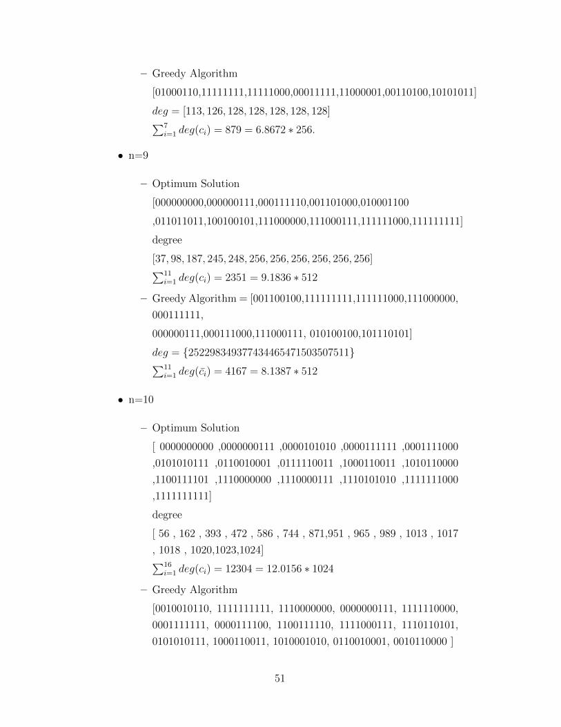
– Greedy Algorithm

[01000110,11111111,11111000,00011111,11000001,00110100,10101011]

deg = [113, 126, 128, 128, 128, 128, 128]∑7i=1 deg(ci) = 879 = 6.8672 ∗ 256.

• n=9

– Optimum Solution

[000000000,000000111,000111110,001101000,010001100

,011011011,100100101,111000000,111000111,111111000,111111111]

degree

[37, 98, 187, 245, 248, 256, 256, 256, 256, 256, 256]∑11i=1 deg(ci) = 2351 = 9.1836 ∗ 512

– Greedy Algorithm = [001100100,111111111,111111000,111000000,

000111111,

000000111,000111000,111000111, 010100100,101110101]

deg = {252298349377434465471503507511}∑11i=1 deg(ci) = 4167 = 8.1387 ∗ 512

• n=10

– Optimum Solution

[ 0000000000 ,0000000111 ,0000101010 ,0000111111 ,0001111000

,0101010111 ,0110010001 ,0111110011 ,1000110011 ,1010110000

,1100111101 ,1110000000 ,1110000111 ,1110101010 ,1111111000

,1111111111]

degree

[ 56 , 162 , 393 , 472 , 586 , 744 , 871,951 , 965 , 989 , 1013 , 1017

, 1018 , 1020,1023,1024]∑16i=1 deg(ci) = 12304 = 12.0156 ∗ 1024

– Greedy Algorithm

[0010010110, 1111111111, 1110000000, 0000000111, 1111110000,

0001111111, 0000111100, 1100111110, 1111000111, 1110110101,

0101010111, 1000110011, 1010001010, 0110010001, 0010110000 ]

51

degree

{56 ,112, 218 ,313, 412, 508, 634, 740 ,823, 896, 938, 978 ,1008,

1022 ,1024 }∑15i=1 deg(ci) = 9682 = 9.4551 ∗ 1024

• n = 11

Greedy Algorithm

[ 00000000000 ,11111111111 ,11111111000 ,00011111111 ,11111000000

,00000011111 ,11000000001 ,11100000111 ,01000000110 ,00000111000

,00110100000 ,10100110000 ,00001010101 ,11000101100 ,00101100011

,11001011111 ,00110011110 ,10101001101 ,10011101010 ,11111001011

,01111001100 ]

Degree=[67 ,134 ,267 ,388 ,520 ,652 ,795 ,965,1120, 1251, 1378 ,1513,

1630, 1728, 1827, 1909, 1960, 2002, 2034, 2044, 2048 ]∑21i=1 deg(ci) = 26232 = 12.8086 ∗ 2048

• n = 12

Greedy Algorithm

[ 000000000000 ,111111111111 ,111000000000 ,000000000111 ,111111000000

,111111111000 ,000111111111 ,000000111111 ,000000111000 ,000111000000

,000111111000 ,111000000111 ,111000111111 ,111111000111 ,110000111100

,001111000011 ,101011111101 ,011110011110 ,111110101010 ,111010111001

,001101110110 ,101110011000 ,011011010000 ,110001100001 ,010100000010

,100101000100 ,000011000110 ,010011101001 ,100000110101 ,110100100110

,100101100111 ,010100010111]

deg=[79, 158, 321, 471, 633, 770, 920, 1056,1292, 1498 1682 1901 2093

2260 2479 2698 2913 3056 3214 3321 3449 3568 3642 3757 3852 3921

3980 4026 4055 4080 4094 4096 ]∑32i=1 deg(ci) = 79335 = 19.3689 ∗ 4096

52

REFERENCES

[1] J. Orth and S. Houghten, “Optimizing the salmon algorithm for theconstruction of dna error-correcting codes.” IEEE Symposium on Com-putational Intelligence in Bioinformatics and Computational Biology.,vol. 17, 2011.

[2] J. Sun, S. Houghten, and J. Ross, “Bounds on edit metric codes withcombinatorial dna constraints.” Congressus Numerantium, vol. 204, pp.65–92, 2010.

[3] V. I. Levenshtein, “Binary codes capable of correcting deletions, in-sertions and reversals,” Soviet Physics - Doklady, vol. 10, no. 8, pp.707–710, February 1966.

[4] F. McWilliams and N. Sloane, The Theory of Error Correcting Codes.Amsterdam, The Netherland, North Holland: North Holland publishingcompany, 1977.

[5] J. D. Ullman, “On the capabilities of codes to correct synchronizationerrors,” IEEE Trans. Inf. Theory, vol. IT-13, no. 1, pp. 95–105, January1967.

[6] N. Sloane, “On single-deletion-correcting codes,” Codes and Designs,Ohio State University, pp. 273–292, May 2002.

[7] T. Swart and H. Ferreira, “A note on double insertion/deletion correct-ing codes,” IEEE Transaction on Information Theory, vol. 49, no. 1, pp.269–273, 2003.

[8] M. Mitzenmacher, “A survey of results for deletion channels and relatedsynchronization channels,” Probab. Surveys, vol. 6, pp. 1–33, 2009.

[9] N. Sloane., “Challenge problems: Independent sets in graphs.” [Online].Available: http://www2.research.att.com/ njas/doc/graphs.html

[10] D. J. M.R. Gary, Computers and interactability: A Guide to the Theoryof NP-Completeness. New York: Freeman, 1979.

53

[11] F. Khajouei, M. Zolghadr, and N. Kiyavash, “An algorithmic approachfor finding deletion correcting codes,” Information Theory Workshop(ITW), 2011 IEEE, pp. 25 –29, oct. 2011.

[12] S. Haykin, Communication Systems. John Wiley and Sons Inc, 2001.

[13] H. Mercier, V. Bhargava, and V. Tarokh, “A survey of error-correctingcodes for channels with symbol synchronization errors,” IEEE Commu-nications Surveys and Tutorials, pp. 87–96, 2010.

[14] R. R. Varshamov and G. M. Tenengol’ts, “Correction code for singleasymmetrical errors,” Automat. Telemekh., vol. 26, pp. 288 – 292, 1965.

[15] A. S. J. Helberg and H. C. Ferreira, “On multiple insertion/deletioncorrecting codes,” IEEE Trans. Inform. Theory, vol. 48, pp. 305–308,January 2002.

[16] S. Butenko, P. Pardalos, I. Sergienko, V. Shylo, and P. Stetsyuk., “Find-ing maximum independent sets in graphs arising from coding theory,”Proceedings of the 2002 ACM Symposium on Applied Computing, pp.542–546, 2002.

[17] R. L. Brooks, “On colouring the nodes of a network,” MathematicalProceedings of the Cambridge Philosophical Society, vol. 37, pp. 194–197, 1941.

[18] V. I. Levenshtein, “Efficient reconstruction of sequences from their sub-sequences or supersequences,” J. Comb. Theory, vol. 93, no. 2, pp. 310– 332, 2001.

[19] P. M. Pardalos and J. Xue, “The maximum clique problem,” Journalof Global Optimization, vol. 4, no. 3, pp. 301–328, 1994-04-01. [Online].Available: http://dx.doi.org/10.1007/BF01098364

[20] N. Z. Shor, “Dual quadratic estimates in polynomial and boolean pro-gramming.” Ann. Oper. Res., vol. 25, no. 1, p. 163168, 1990.

[21] P. M. Pardalos and G. P. Rodgers., “A branch and bound algorithm forthe maximum clique problem.” Computers Ops Res., vol. 19, p. 363375,1992.

[22] J. Abello, S. Butenko, P. Pardalos, and M. Resende, “Finding indepen-dent sets in a graph using continuous multivariable polynomial formu-lations,” Journal of Global Optimization, vol. 21, no. 2, pp. 111–137,2001.

[23] T. S. Motzkin and E. G. Straus., “Maxima for graphs and a new proofof a theorem of turan.” Canad. J. Math., vol. 17, p. 533540, 1965.

54

[24] R. L. R. Thomas H. Cormen, Charles E. Leiserson, Introduction to al-gorithms. MIT Press / McGraw-Hill., 1990.

55