by wang jiahao
TRANSCRIPT

1
Autonomous driving car model and its
control By
Wang JiaHao
A Thesis Submitted in Fulfillment
of the Requirements for the Degree of
MASTER OF
AUTOMOTIVE ENGINEERING
TUTOR:
Professor Nicola Amati
POLITECNICO DI TORION

2
Abstract
This thesis work focused on the research of the autonomous driving
car model and of the steering and speed control of autonomous vehicles.
The different level of vehicle dynamic model are considered such as
kinematic model and bicycle model with the linear or nonlinear tire
model.
The controller is split in 2 parts, the first one is longitudinal controller
corresponding to change of speed, and the other is lateral one which is
mainly related to the steering angle. The lateral controller is based on
the MPC theory, and the longitudinal one use the PID theory. The entire
controller, which is developed in the matlab and simulink, should work
well simultaneously to follow the desired path. To test it, the different
scenario is generated by the autonomous driving toolbox in matlab.
To get more reliable data of the vehicle state, we are using the Carsim
software co-simulating with matlab, making our consideration more
comprehensive.
It’s important to see how the controller parameters (step horizon, cost
function) have the effect on the results.

3
Content
Content ...................................................................................................................................... 3
Chapter 1 Introduction: ............................................................................................................. 6
1.1 General idea of autonomous driving car ......................................................................... 6
1.2 MPC for path planning and tracking application. .......................................................... 11
1.3 thesis problem statement ............................................................................................. 13
Chapter 2 Vehicle and tire model ............................................................................................ 14
2.1 kinematic model ............................................................................................................ 15
2.2 dynamic model .............................................................................................................. 18
2.2.1 bicycle model .......................................................................................................... 19
2.2.2 Tire model ............................................................................................................... 22
2.2.3 linear bicycle model. ............................................................................................... 25
Chapter 3 MPC controller for lateral control .......................................................................... 26
3.1 overview of model predictive control ........................................................................... 26
3.2 LTI model predictive control algorithm ......................................................................... 29
3.3Nonlinear model predictive control ............................................................................... 34
3.4 numerical method for nonlinear system ....................................................................... 36
3.5 dynamic model in path coordinate ............................................................................... 38
Chapter4 Longitudinal control................................................................................................. 40
4.1 Overview of PID theory ................................................................................................. 40
4.2 introduction of longitudinal control .............................................................................. 43
4.3 desired velocity generation ........................................................................................... 45
4.4 Coupled effect between longitudinal and lateral direction. ......................................... 47
Chapter 5 Results ..................................................................................................................... 52
5.1 simulink environment .................................................................................................... 53
5.2 cooperation simulation with carsim .............................................................................. 57

4
5.3 Benchmarking with Carsim ............................................................................................ 61
5.4performance and final result plots ................................................................................. 65
5.4.1 lane keeping assistant system only with lateral control ........................................ 65
5.4.2 lane keeping assistant system with both longitudinal and lateral control. ........... 67
5.4.3 benchmarking with Carsim ..................................................................................... 70
Reference ................................................................................................................................ 72

5
LIST OF FIGURES
figure 1 vehicle control........................................................................................................... 9
figure 2 kinematic model ..................................................................................................... 15
figure 3 bicycle model .......................................................................................................... 19
figure 4 lateral force ............................................................................................................. 23
figure 5 longitudinal force .................................................................................................... 23
figure 6 linear tire force ....................................................................................................... 24
figure 7 mpc algorithm ...................................................................................................... 27
figure 8 MPC controller ..................................................................................................... 28
figure 9 PID control .............................................................................................................. 41
figure 10 force distribution in 4 wheels ............................................................................... 45
figure 11 frication coefficient as function of slip ratio ......................................................... 47
figure 12 longitudinal and lateral force based on experiment data .................................. 48
figure 13 elliptical model...................................................................................................... 49
figure 14 sequence of longitudinal control .......................................................................... 50
figure 15 total architecture of control algorithm ................................................................. 51
figure 16 total simulink environment ................................................................................... 53
figure 17 lateral deviation and relative yaw angle ............................................................... 54
figure 18 vehicle and environment part ............................................................................... 55
figure 19 different scenario .................................................................................................. 57
figure 20 carsim configuration ............................................................................................. 58
figure 21 vehicle dimension ................................................................................................. 59
figure 22 input set ................................................................................................................ 59
figure 23 output set ............................................................................................................. 60
figure 24 carsim s-function .................................................................................................. 61
figure 25 carsim lane keeping function ................................................................................ 61
figure 26 acceleration constraints ........................................................................................ 62
figure 27 preview length ................................................................................................... 63
figure 29 scenario in matlab ................................................................................................ 64
figure 28 scenario in carsim ................................................................................................. 64
figure 30 performance plot A ............................................................................................... 66
figure 31 performance plot B ............................................................................................... 69
figure 32 benchmarking reslts comparision ......................................................................... 71

6
Chapter 1 Introduction:
1.1 General idea of autonomous driving
car
Autonomous driving car is the car that fulfills the transportation task
without the human intervention, using the computer inside the car to
simulate the behavior of the driver and make decision.
Getting the environment data from the variety of sensor, based on the
information of road, localization of vehicle, and the obstacle the
controller will give the command.
Here the autonomous driving system can be divided by the 4 parts
which is system management, environment sensing, path planning, and
vehicle control.
(1) environment sensing
The same as the human driving car, autonomous driving car need the
information of driving environment in real time. There are 2 ways to get
the data, the one is by the help of all the sensor inside the vehicle ,
combined with the environment to have sensor fusion, trying to let
vehicle ‘understand ’ the environment, the other is through the internet
to supply the data of the outside area. For example by the vehicular
networking vehicle can easily get the road data in front of it also the
driving trend of the car which is around the autonomous driving car.

7
Environment sensing system uses these data correlating with the
model inside the computer to understand and recognize the situation.
Environment sensing system is key parts to have reliable driving
behavior which means it is also the most difficult part to fulfill. As we all
know to drive in the city at least autonomous driving car need recognize
the road the traffic light and all the traffic sigh related to traffic rules.
Getting the data from environment sensing system transfer it to path
planning system.
(2)Path planning system
Path planning means inside the environment which has obstacle,
based on a certain standard such as minimal the length of path or
minimal the energy to be used, finding a path from starting point to the
final destination without any interruption.
At present path planting system mainly used theory coming from
research about robotics. In general there are 2 parts: global path
planning and local path planning.
Global path planning means under the condition of knowing the total
map of environment, using the local environment information such as
the location of obstacle and the boundary of the road, autonomous
driving car can confirm the optimist path to follow.
But when the condition is changing such as the other car interrupt

8
the path that autonomous driving car followed, it is important to use the
local path planning to re-plan the path. Local path planning, which
according to sensor data representing local environment information,
generate the path need to be followed. It is under the guide of global
path planning; In the process of planning consider not only the minimal
energy to be used, safety issues but also problem of dynamic
environment constraints.
In the process of local path planning another issue should pay
attention to is the motion planning, which means that local path should
consider the constraint of vehicle dynamic.
Using model predictive control theory into autonomous driving path
planning process, the important issue is that how to solve the vehicle
dynamic constraints. We will discuss it in the following chapter.

9
(3) vehicle control system
Vehicle control system, in which include longitudinal and lateral
direction control, generate the command to follow the path coming from
path planning system. The same as the robotic control there is difference
between the path and the trajectory. Trajectory which considers space
and time simultaneously is one kind of path. The essence of path
planning is trying to minimal the error between the vehicle location and
the reference trajectory through control of vehicle motion. If we talk
about the trajectory it also includes error within time.
Vehicle control system is important part of autonomous driving car.
Environment sensing, path planning must integrate with vehicle control
system. Under all the condition of driving, especially with very high
speed, vehicle dynamic has much more effect on the results. All the
parameter such as side slip of the vehicle, the friction coefficient
figure 1 vehicle control

10
between the tire and the road, aerodynamic need to consider compared
with low speed condition.
(4)system management
Autonomous driving car first is a system work, in which there are a lot
of sensors, actuators, and electronic control unit need to work together,
to fulfill variety of functions such as car following, lane keeping,
emergency stopping, and obstacle avoidance. Different function need to
cooperate with different sensor and actuators to make sure the safety
and comfortable regulation.
When the new condition is facing or the autonomous driving car
receive the new requirement from the passage the system management
should assign different function to actuators based on data coming from
different sensor.
At the same time system management should supervise the whole
autonomous driving car to check what kind of situation of the parts
inside the car.

11
1.2 MPC for path planning and tracking
application.
Vehicle dynamic model play an important role in solving the problem
of autonomous driving car path planning and tracking. Introducing the
dynamic model in path planning process could increase the real-time
capability by reducing the computation quantity.
Felipe KUHNE purpose a control scheme based on vehicle kinematic
model for wheeled mobile robot. Using MPC to have better constraints
condition, by the help of Quadratic programming (QP) to handle
linearization problem of wheeled mobile robot model.[1]
Razvan.C.Rafaila consider autonomous driving car model with
dynamic model but take in to account the nonlinear tire force. The
nonlinear model predictive control model use optimization algorithm to
have the minimal value of cost function.[2]
Matthew Brown put the local path planning and path tracking in same
control system using model predictive control. All the results must be
generated before calculation which takes into account the desired path
positioned in two safe envelopes.
The one envelope represents stability problem optimization the other
gives indicator of obstacle avoidance.[3]

12
Jonathan Y.Goh generates insight from professional drivers. They give
an approach to control autonomous drifting to have better performance
of path tracking problem.
The reference path is generated point by point from all the equilibrium
of drifting points considering the side slip angle of tire is no more very
small meaning non linear of tire force.[4]
Jiechao LIU investigates the effect of different degree of freedom on
performance of model predictive controller. The indicators such as time
to reach the target point and the deviation from desired path are used to
judge the performance.[5]
Steven C peters design path tracking controller consider differential
flatness to explore the limits of tire force with better performance in
trajectory tracking problem.[6]
Path following problem is formed to geometry way to design the
control algorithm [7-11], it is important to consider the closed loop
controller including both longitudinal and lateral direction.[12],and the
driver model detailed information in paper[13 14].

13
1.3 thesis problem statement
This thesis tries to investigate the application of model predictive
control (MPC) in autonomous driving car. Starting from the vehicle
kinematic and dynamic model building within linear or nonlinear tire
model, following the discussion of concepts about the model predictive
control such as optimization, cost function, quadratic programming and
constraints.
A nonlinear mathematical model for a vehicle with dynamic constrains
is developed based on the vehicle data coming from Carsim. Test in the
simulink with various kinds of scenarios to see the final performance of
the controller. Carsim vehicle model is embedded as simulink s-function
and controller is designed by the help of matlab mpc toolbox.
An important issue should be specified which is prediction horizon; it
is the main parameter in mpc controller. The prediction horizon
influences the final performance of the controller and the computation
cost. For autonomous driving car it is quiet important to fulfill the path
tracking in real time, otherwise the vehicle is easily to meet the
dangerous situation due to the delay of the time.
14
Chapter 2 Vehicle and tire
model
Autonomous driving car need to know the car model such as kinematic
or dynamic model to fulfill the function of path planning and path
tracking. From the first chapter we have insight that the better known of
vehicle dynamic model especially when design the path planning system
putting dynamic model in it, the better the path tracking results will
present. It means that the reliable vehicle model is not only precondition
of designing of mpc controller, but also basement of path tracking.
When design mpc controller it is important to consider driving
situation of autonomous driving car. In order to have proper
autonomous driving motion control we must choose proper variable to
have precise prediction of vehicle motion changing.
Motion of vehicle on the road is very complicated, in order to have
right descriptions of car motion; one of the useful approaches is complex
system of differential equations, choosing different variable representing
motion of car.
Adding vehicle kinematic or dynamic model inside mpc controller, we
can confirm aim of control for the controller. Especially in motion
planning, by the help of linearization and simplification of vehicle model,
15
requirement of real time performance can be met.
The linearization and simplification are important approach to solve
the car model such as tire elliptical model and point mass model of car.
In this chapter we present some models of the car, their assumptions
and constraints.
2.1 kinematic model
Kinematic is kind of theory represents the motion of points and
group of objects, neglecting the force that have effects on the motion.
Kinematic is always in direction of geometry of motion to make the
research, considering as a branch of mathematics. Kinematics problem
begins by describing the geometry of the system and declaring the initial
conditions of any known values of position, velocity and/or acceleration
of points within the system.[1]
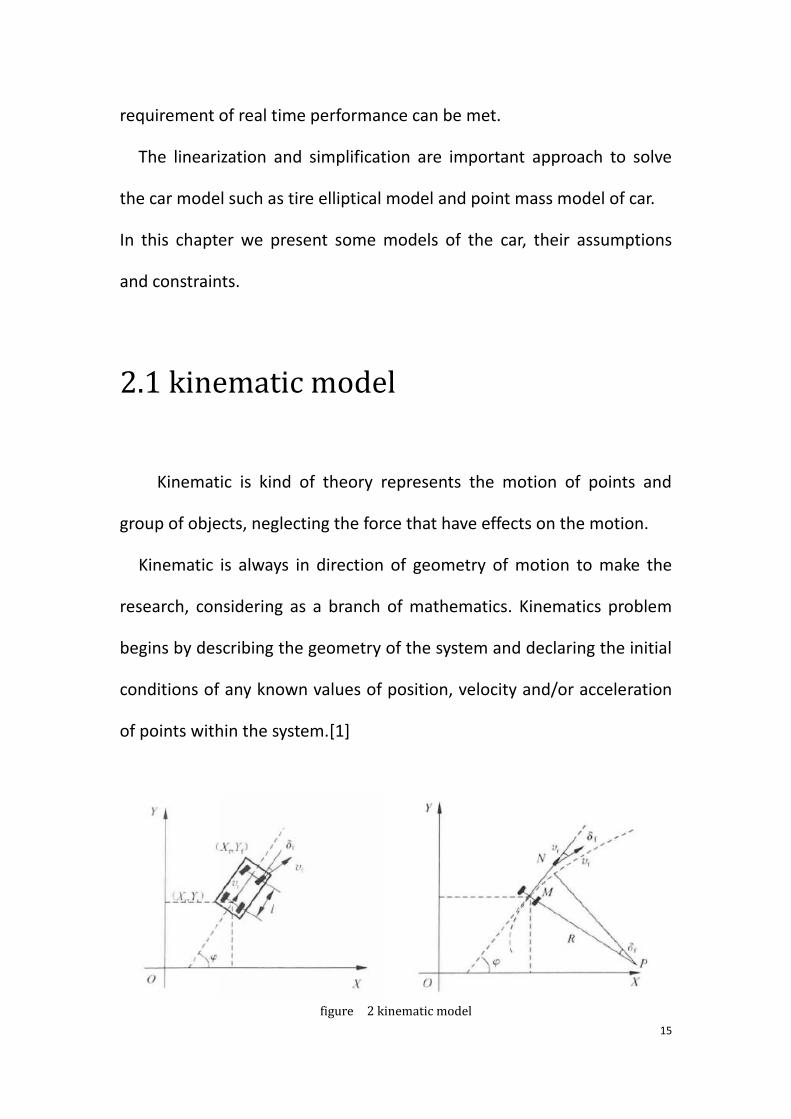
figure 2 kinematic model

16
As figure 2. showed, represent the coordinate of center
point of front axles and rear axles, represent yaw angle of vehicle,
is steering angle of front axle, rear axle, is speed of
front axle, l is wheel base of vehicle.
R is radius of trajectory of the center of mass of rear wheel, P is
Instantaneous center of rotation, M is center point of rear axle, N is
center point of rear axle.
At the center point of rear axle M, the speed is:
The kinematic constrains of front and rear axles are:
=0
Combined with the upper 2 parts of formula we can get:
Considering the geometry relation of front and rear axles:
the yaw rate is :

17
is yaw rate of the car, at the same time from yaw rate the radius of
curvature R and steering angle of front axle can get:
Finally the kinematic model is :
=
The model can be described in a more uniform way which is state
space matrix. Here state variable is [ ] and the control variable is
[ ]. The new model is :
=
+

18
2.2 dynamic model
Vehicle dynamic mainly used to analysis the vehicle suspension
effect including quarter car model and the drivability of car. In drivability
analysis focused on the longitudinal and lateral dynamic issues.[15]
In this thesis we want use mpc controller finishes the path tracking
function, as well as to simplify vehicle dynamic model to reduce
computation cost, in order to confirm real time.[16]
Using kinematic model is not reliable especially when the speeds are
increased and path curvatures are changing. But in such condition,
dynamic model has good performance in path tracking performance.
The dynamic model of the car is very complicated and has more
degree of freedom to handle. At the same time the system is nonlinear
discontinuous.
Before build vehicle dynamic model we need purpose some ideal
assumption:
1. The road is considered as flat surface, the motion is planar.
2. Neglect the effect of motion of suspension
3. Consider the linear tire model neglecting decoupled effect in 2
directions.

19
4. The load transfer is not into consideration
5. Neglect aerodynamic force.
2.2.1 bicycle model
Based on above 5 ideal assumptions, there are 3 direction of motion
for planar vehicle which are longitudinal, lateral and yaw motion of the
car.
As illustrated in figure 3, coordinate system oxyz is fixed in the vehicle;
xoz is midplane of left and right. The original point is in center of gravity
of the car. Coordinate system OXY fixed in the road.
About the force in figure:
are the longitudinal force of front and rear tire
are the lateral force of front and rear tire
figure 3 bicycle model

20
are the tire force in x direction
are the tire force in y direction
Applying Newton’s second law of motion along the X-axis ,Y-axis and Z-
axis:
+
+
Where m and denote the vehicle mass and yaw inertia,
respectively. and denote vehicle longitudinal and lateral velocities,
respectively, and is the turning rate around a vertical axis at the
vehicle’s centre of gravity.
The longitudinal and lateral tire force components in the vehicle body
frame are modeled as follows:
The longitudinal and lateral tire forces are given by Pacejka’s model.
They are nonlinear functions of the tire slip angles α,slip ratios σ, normal
forces Fz and friction coefficient between the tire and road μ:
Fl = fl(α, σ, Fz, μ),

21
Fc = fc(α, σ, Fz, μ).
The slip angles are defined as follows:
where the tire lateral and longitudinal velocity components are
computed from:
The velocity component can be calculated from:
The slip ratios s is approximated as follows:
The friction coefficient μ is assumed to be a known constant and is
the same at all four wheels. We use the static weight distribution to
estimate the normal force on the wheels. They are approximated as:
Finally consider the vehicle fixed coordinate system and inertial
frame.

22
2.2.2 Tire model
Making research on vehicle dynamic, the longitudinal and lateral force
with aligning torque has effect on drivability and handling stability. Due
to the reason of complex behavior of tire, the dynamic model is non
linear. So the important issue to generate dynamic model is choosing
reliable and useful tire model.
Pacejka purposes the magic formula which uses trigonometric
function to represent longitudinal and lateral force [22 23]. Finding
relationship between side slip angel and force in different direction, the
characteristics of tire can be presented.
The usual form of magic formula is:
Where Y is output of function which can be longitudinal or lateral tire
force. B,C,D,Sv are the coefficients correlate to the experiment data. In
the following part we show some typical example of tire plots using
pacejka formula.
Figure 4 shows the lateral tire force as function of side slip angle at
different value of friction coefficient.
Figure 5 shows the longitudinal tire force as function of slip ratio at
different value of friction coefficient.

23
Using pacejka formula for controller designed is also too much
figure 4 lateral force
figure 5 longitudinal force

24
complicated, which means the more simplified model needs to be
presented. From the figure we can easily find that based on the
assumption of side slip angle or slip ratio is very small, the tire force is in
the linear region. The formula can be changed to:
Where is cornering stiffness coefficient of tire, it is related to
frication coefficient and normal force .
Figure6 shows difference between pacejka model and linear model.
The linear tire model is the simplest one which can be used in dynamic
model to design mpc controller without damage to the performance of
path tracking.
figure 6 linear tire force

25
2.2.3 linear bicycle model.
To linear dynamic model, based on the small angle assumption,
approximate all trigonometric function using first order Taylor expansion:
After that the side slip angle are:
,
Combined equations ,the lateral tire force are:
Substitute the equation we get the linear dynamic equation.
26
Chapter 3 MPC controller
for lateral control
This chapter the general knowledge of mpc is presented to show the
reason why that the controller is using mpc theory. Following section is
to show an example of simple controller tracking a desired path. Inside
controller the vehicle model is kinematic model because the reduction of
complexity at first.
The rest of this chapter is to illustrate the controller that used
commonly to fulfill path tracking function based on dynamic vehicle
model.[17 18 19 20 21 ]
3.1 overview of model predictive control
MPC is a method to control process with a variety of constrains.
Chemical industry firstly introduce to factory since 1980s. Nowadays the
use of this control theory has expanded to power electronics and
autonomous driving car, because of the advantage of current timeslot
optimization while keeping future time slots in account.
Inside mpc control process there are 3 critical steps: prediction model,
rolling optimization and feedback correction.

27
Model Predictive Control optimizes the output of a plant over a finite
horizon in an iterative manner (Refer to Figure 7). At time step k, the
initial value of current plant state is known, the control input is
calculated for finite time steps in future k = t + 0T; t + 1T; :::; t +
pT ,where p is previewed prediction horizon steps. During calculation the
problem has transferred to an open loop, constrained, finite time one.
In practical situations, only the first value of control sequence could be
the input to the system. Because of the model simplification and added
disturbances or other kind of noise which can cause error between the
predicted output and the actual process output.
Thus only the first step of the control strategy is applied to the plant
and the plant state is measured again to be used as the initial state for
the next time step. This feedback of the measurement information to
figure 7 mpc algorithm

28
the optimizer adds robustness to the control. The plant state is sampled
again and the whole process is repeated again with the newly acquired
states. The prediction time window [t + 0T; t + 1T; :::; t + pT ] shifts
forward at every time step (reason why MPC is also known as Receding
Horizon Control.
Figure8 shows that general mpc used for autonomous driving car.
The 3 main components are dynamic optimizer, the vehicle model, and
the cost function and constraints.
The output from the mpc controller will be the input to the vehicle;
here mpc controller is for lateral control which means the output is
steering angle. Usually to control a vehicle we need also 2 more
parameter the throttle and the brake which will be discussed in next
chapter. The ground vehicle can be simulated in simulink by a block. The
state estimator gives all the indication of the vehicle in which represents
all state of vehicle. The output of this block will be the input to mpc as
figure 8 MPC controller
29
the new initial condition of next time step calculation.
The task of sensor is to give information of environment which may be
the boundaries of 2 roads, the position of obstacle, and the presence of
other cars.
3.2 LTI model predictive control
algorithm
LTI model prediction control algorithm is based on LTI model as
prediction model which is also common used model in model predictive
control. Compared with nonlinear model predictive control the
advantage is that computation is simple and better real time
performance. For autonomous driving car the real time performance of
algorithm is important issue to consider. Due to that reason here the
introduction of LTI model predictive control algorithm is presented.
As said before in following parts we divide 3 topics to discuss:
prediction function, optimization solution and feedback.
(1)prediction function:
Consider following discrete linear model:

30
We can set as :
A new state space equation:
All the matrix is defined as:
In order to simplify calculation, purpose assumption:
Considering prediction horizon is Np, control horizon is Nc. The output of
control sequence and the output of system in prediction horizon is
calculated by:
31
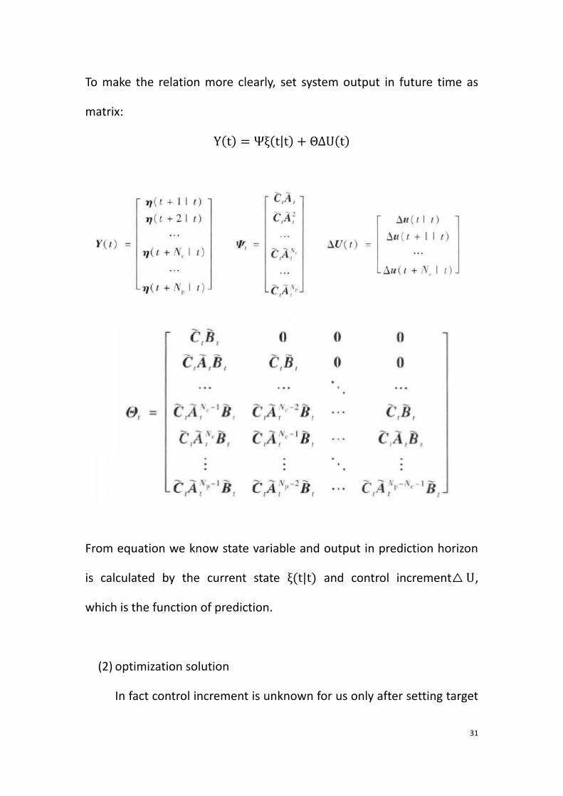
To make the relation more clearly, set system output in future time as
matrix:
From equation we know state variable and output in prediction horizon
is calculated by the current state and control increment ,
which is the function of prediction.
(2) optimization solution
In fact control increment is unknown for us only after setting target
32
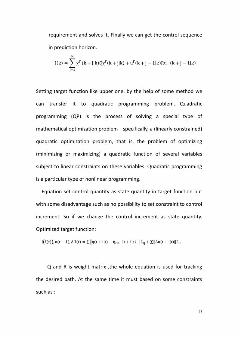
requirement and solves it. Finally we can get the control sequence
in prediction horizon.
Setting target function like upper one, by the help of some method we
can transfer it to quadratic programming problem. Quadratic
programming (QP) is the process of solving a special type of
mathematical optimization problem—specifically, a (linearly constrained)
quadratic optimization problem, that is, the problem of optimizing
(minimizing or maximizing) a quadratic function of several variables
subject to linear constraints on these variables. Quadratic programming
is a particular type of nonlinear programming.
Equation set control quantity as state quantity in target function but
with some disadvantage such as no possibility to set constraint to control
increment. So if we change the control increment as state quantity.
Optimized target function:
( )
Q and R is weight matrix ,the whole equation is used for tracking
the desired path. At the same time it must based on some constraints
such as :

33
Control quantity constraint:
Control increment constraint:
Output constraint:
From here the whole optimization solution is finished, solving all these
equation with different constraints, the control sequence in future time
can be calculated.
(3) Feedback
After solving all the equation, the control increment sequence in
future time :
Based on model predictive control theory, setting the first one in the
sequence as the input control to the system.
The system execute control input till next time step. In next time step the
system based on current information predict future output.

34
3.3Nonlinear model predictive control
In order to use linear model predictive control, the first requirement
is to have linearized vehicle dynamic model. Apart from the nonlinear
model predictive, linear model predictive control is a second choice. As
the research is going on, nonlinear model predictive control is used in
more common area.
For a nonlinear system, consider the model like that:
Where f is transfer function of system, is n dimensional state variable
is m dimensional control variable, is state vatiable constraint, is
control variable constraint.
Set f(0,0)is a stable point of system, and also the control target of
system. For any time horizon N, consider following target function
Where U(t) is control sequence in horizon N, is all the state variable
sequence under control input sequence. Inside the target function
the first item represents tracking ability, the second item presents
constraints.
Combined with model and target function, nonlinear model predictive
control is to solve the problem under all kind of constraints in every time

35
step. For example:
If we get the results from equation satisfy all requirement and constrains,
the optimal control sequence U(t) will meet. Based on the model
predictive control theory, setting the first item, which is inside the
control sequence, as input to the controlled system.
In next time step, system gets new current state and solves the
equation; continue setting first item as input to system. For any
nonlinear system during calculation there are N(n+m) variable, n
nonlinear constraints, also including control increment constraints and
output constraints.
So the more dof of dynamic system the more calculation power
needed. In our case vehicle dynamic model is 3 dof model, the
advantage of nonlinear model predictive control is still there. Otherwise
for high dof vehicle model it needs some simplification, to obey the
requirement in real time.
36
3.4 numerical method for nonlinear
system
In nonlinear model predictive control, by the nonlinear model,
current state and control sequence, predict the future state of system.
It is an iteration process, but with unknown control sequence. Due to
that reason it needs an iteration equation to have an approximate
solution of differential equation.
Usually there are 2 methods, one is Euler method, and the other is
Runge-Kutta method.
The Euler method (also called forward Euler method) is a first-order
numerical procedure for solving ordinary differential equations (ODEs)
with a given initial value. It is the most basic explicit method for
numerical integration of ordinary differential equations.
The Euler method is a first-order method, which means that the local
error (error per step) is proportional to the square of the step size, and
the global error (error at a given time) is proportional to the step size.
The Euler method often serves as the basis to construct more complex
methods.
For a differential equation:

37
Using Euler method, the result in time n+1 can be calculated from
time n. the iteration equation is
But usually this method has a very low level of precision. So in some
condition we try to use another method.
the Runge–Kutta methods are a family of implicit and explicit iterative
methods, which include the well-known routine called the Euler Method,
used in temporal discretization for the approximate solutions of ordinary
differential equations.
Usually the method is :
Here one important issue needs to be specify, the more precision the
results we require, the lower the computation speed.
38
3.5 dynamic model in path coordinate
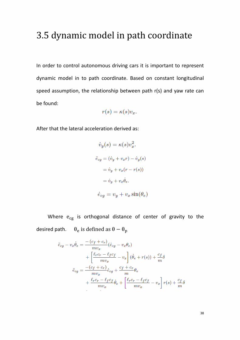
In order to control autonomous driving cars it is important to represent
dynamic model in to path coordinate. Based on constant longitudinal
speed assumption, the relationship between path r(s) and yaw rate can
be found:
After that the lateral acceleration derived as:
Where is orthogonal distance of center of gravity to the
desired path.

39
The state space model in tracking error variables is therefore given by:
40
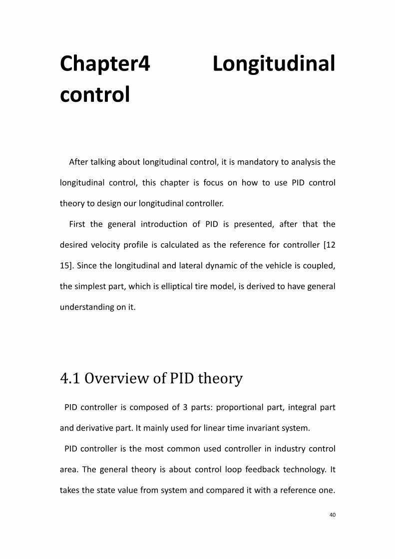
Chapter4 Longitudinal
control
After talking about longitudinal control, it is mandatory to analysis the
longitudinal control, this chapter is focus on how to use PID control
theory to design our longitudinal controller.
First the general introduction of PID is presented, after that the
desired velocity profile is calculated as the reference for controller [12
15]. Since the longitudinal and lateral dynamic of the vehicle is coupled,
the simplest part, which is elliptical tire model, is derived to have general
understanding on it.
4.1 Overview of PID theory
PID controller is composed of 3 parts: proportional part, integral part
and derivative part. It mainly used for linear time invariant system.
PID controller is the most common used controller in industry control
area. The general theory is about control loop feedback technology. It
takes the state value from system and compared it with a reference one.
41
Based on this error applies a correction take in to account proportional,
integral, and derivative terms (denoted P, I, and D respectively), hence
the name.
The main target of controller is to let the output of system as same as
the desired value. PID controller adjusts input according to the history
data and error to make system more stable.
In some application there is no mandatory to use all 3 parts of
controller. Usually sometimes only PI or PD or only P parts are presented
in controller.
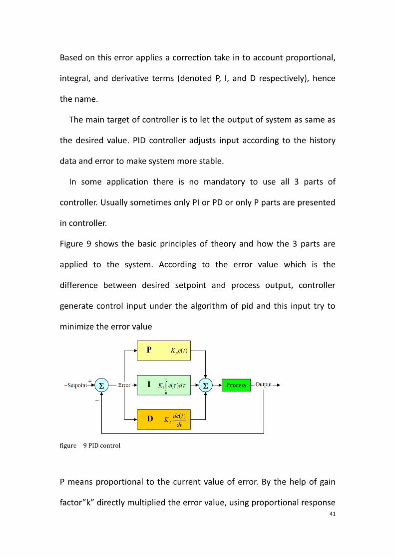
Figure 9 shows the basic principles of theory and how the 3 parts are
applied to the system. According to the error value which is the
difference between desired setpoint and process output, controller
generate control input under the algorithm of pid and this input try to
minimize the error value
figure 9 PID control
P means proportional to the current value of error. By the help of gain
factor”k” directly multiplied the error value, using proportional response

42
to compensate system.
I is represents past value of error and integrate it them over time. Due
to the condition that after proportional control there is a still the error
between current state and desired one which is called residual error. The
I parts try to eliminate residual error. When the residual error turn to be
0, the integral will not continue increase.
D is a part taking in to account the future trend of error. By the help of
derivation of error value, the mission of this part is to reduce change rate
of error value to make it more stable.
The total function can be expressed as :
Where denote as proportional terms, denote as integral terms
and denote as derivative part.

43
4.2 introduction of longitudinal control
After talking about the lateral control of the autonomous driving
cars, it is also important to spend time in longitudinal control, since that
the vehicle can’t drive with constant speed.
These days a lot of work and research has developed to solve
challenge in security problem hence that even in today there are also
millions of people are injured because of car accident. It is the reason
that every car maker is trying to use ADAS to reduce this big number. In
other words the ADAS is also the low level of autonomous driving cars.
One of the common used method is that multi point preview
model[24], this model divide the desired path ahead of vehicle to some
points based on the deviation between the point and current lane
generate signal of steering angle and throttle/ brake.
An active cruise control (ACC) is also used by a majority of vehicles.
The main target is to keep vehicle speed and safety distance between
cars. An mpc based control algorithm is generated [25] with the
advantage of minimal fuel consumption.
Since the vehicle is a system work that every parts have deeply
relationship with each other.
Here we just specify some important parts such as:
The longitudinal and lateral motions are kinematic and dynamic

44
coupling, because of the yaw motion.
When the vehicle is accelerating or cornering, there are longitudinal
and lateral accelerations. Due to that the load transfer is happening and
the vehicle is no more in static state.
The constraint of tire force which called the elliptical model of the tire
is coupled in longitudinal and lateral direction.
It is complex to consider all the effects simultaneously. It is necessary
to have a nonlinear dynamic model to capture all the effects. Since in the
lateral controller which is developed base on mpc theory spends a lot of
time to do calculation. If in longitudinal controller also the nonlinear
model is used which will be a big challenge for the data processor inside
the car. While the real time performance is the first priority of total
system.
Due to the reason of simplification, here the longitudinal controller is
developed by PID theory, using the previewed curvature of path in front
of vehicle, getting data from camera, calculating the desired velocity
while cornering. Here the lateral and longitudinal coupled effects have
effects on the maximal friction force of tire. Based on the desired
velocity and current one, The output of longitudinal controller is signal of
throttle or brake pedal to simulate the driver and it is convenient to
directly send this signal to ECU inside autonomous driving cars.

45
4.3 desired velocity generation
When the vehicle is cornering, it is important to clearly know the
relationship between the steering angel and centrifugal force. If the tire
cannot generate enough force to balance the centrifugal and
aerodynamic force, the vehicle will out of the control which we called
under steering/over steering.
figure 10 force distribution in 4 wheels
From figure 10 shows:we assume that the vehicle is driving in flat road
and neglect aerodynamic force because that the simple model we want
to have.
Taking into account the centrifugal force and tire frication force in
direction to finish the equilibrium equation.

46
Here we assume are conflated with the tire lateral cornering
force . The vertical force on each tire are assumed to be equal which
means all the tire have same frication coefficient . Based on all these
assumption, the approach is referred to ideal steering.
Combined with all the upper equation
Where k denotes the curvature of road. Thus finally we can get the
desired velocity:
To make conclusion of this section, from curvature of the road the
maximal velocity is calculated. It is one of the constraints of longitudinal
controller otherwise the vehicle will go out of the lanes.
The maximal velocity is reference speed of PID controller, time by time
the controlled calculated the error between current speed and maximal
one. Based on the error controller generate signal of throttle/brake

47
pedal to control the speed of the car.
4.4 Coupled effect between longitudinal
and lateral direction.
After getting the maximal velocity, it is mandatory to make research
on the relationship between coupled effect of longitudinal and lateral
direction. In the past the force is generated separately, only the lateral
force to control of the steer of the vehicle and investigate the
performance of autonomous driving cars.
But now due to the presence of longitudinal controller, the tire forces
are generated in both directions at the same time. The condition itself is
changed and the constraints and relationship need to investigate to
make sure the good results.
From the research when increase the longitudinal force of the tire that
figure 11 frication coefficient as function of slip ratio
48
has certain side slip angle, the force in lateral direction is decreases. The
result is same as showed in figure11
By applying the driving or braking torque to the tire with a certain side
slip angle, the shape of frication coefficient is changed along different
side slip angle.
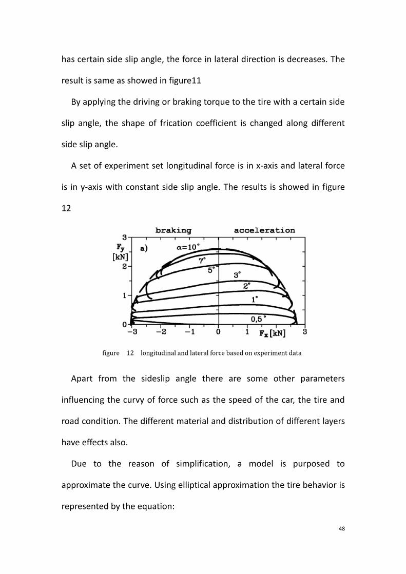
A set of experiment set longitudinal force is in x-axis and lateral force
is in y-axis with constant side slip angle. The results is showed in figure
12
Apart from the sideslip angle there are some other parameters
influencing the curvy of force such as the speed of the car, the tire and
road condition. The different material and distribution of different layers
have effects also.
Due to the reason of simplification, a model is purposed to
approximate the curve. Using elliptical approximation the tire behavior is
represented by the equation:
figure 12 longitudinal and lateral force based on experiment data

49
Where are the lateral force at the given side slip angle with no
longitudinal force applied. The is maximal longitudinal force with
no lateral force which means no side slip angle
Using cornering stiffness substitute lateral force:
Finally the elliptical model of tire is generated to show the couple effect
of lateral and longitudinal direction in figure 13
figure 13 elliptical model
Based on the output of mpc controller, the steering angle and side slip
angle of tire, the lateral force need to apply to the tire is calculated by:

50
From lateral force substitute it in to elliptical model; the available
longitudinal force is generated. The available longitudinal force divide
the mass of the vehicle is the acceleration limit of the vehicle. The limit is
another constraint of PID controller.
figure 14 sequence of longitudinal control
In figure14 it presents the sequence of the data. Starting from the lane
center estimate block, which will be discussed detailed in next chapter,
the curvature of the path is calculated. After due to the prediction
characteristic of mpc controller, the previewed curvature is current
curvature plus the value that curvature derivative multiplies the
prediction horizon. Based on the maximal previewed curvature the
maximal reference velocity is generated, sending it to the PID controller,
according to the difference between the desired velocity and current

51
velocity, the output is acceleration signal. The saturation rate limit
considers maximal longitudinal force available applied to the tire. Taking
in to account the couple effect in 2 directions, the system put first
priority into lateral control otherwise the vehicle will go out of the lanes.
Inside linear model longitudinal dynamic block, by the help of simple
transfer function, the input signal which is acceleration transfers to
output signal which is speed. Using this speed re-send it to mpc
controller updates all the sate inside model. The total architecture of
longitudinal and lateral controller is showed in following figure.
figure 15 total architecture of control algorithm
52
Chapter 5 Results
This chapter introduces the simulation environment based on matlab
and simulink to show the general function of blocks. The test bench
developed in simulink by the help of some example provided by Matlab
Company. It is a basement for our process giving the opportunity to test
the control algorithm performance.
Carsim model is also as s-function introduced to our system because
that it is more comprehensive model taking into account the
aerodynamic force and some dynamic effects of the vehicle. Let the
performance more reliable.
Here first we show the results only with mpc controller to see the
performance about the autonomous driving car in constant speed.
Second Carsim math model representing the whole vehicle system is
introduced into simulink, to see the effects of vehicle dynamic such as
load transfer. After that the results is related to condition including
both longitudinal and lateral controller.
Inside Carsim it provides a procedure of lane keeping function which is
same as our project. It provides an opportunity to have benchmarking
with Carsim. The same scenario is generated both in Carsim and simulink.
The results from 2 methods are compared.

53
5.1 simulink environment
Using matlab to simulate the autonomous driving cars is because that
the powerful computation model and a variety of toolbox that can be
directly used in our project, such as model predictive control toolbox and
automated driving system toolbox.
The automated driving system toolbox provides algorithms and tools
to design and simulate autonomous driving systems. The system give
possibility to generate different scenario including all traffic information,
simulate the entire sensor that embedded in the car and deal with data.
figure 16 presents the total environment of our simulink model which
can be divided into some parts. As discussed before there are
figure 16 total simulink environment

54
longitudinal and lateral control parts, the vehicle and environment parts,
estimate lane center part to simulate the sensor getting the data of
vehicle path.
The general ideal of our system is to keep the vehicle in its lane and
follow the curved road by controlling the front steering angle. This goal is
achieved by driving the lateral deviation e1 and the relative yaw angle e2
to be small. As figure 17 shows:
Controller calculates a steering angle for the ego car based on the
following inputs:
1. Previewed curvature (derived from Lane Detections)
2. Ego longitudinal velocity
3. Lateral deviation (derived from Lane Detections)
4. Relative yaw angle (derived from Lane Detections)
figure 17 lateral deviation and relative yaw angle

55
Using the function representing the vehicle dynamic model, giving the
steering angle and the longitudinal velocity, we can have the vehicle
state during driving. The output can be:
1. Longitudinal position of the car(X coordinate)
2. Lateral position(Y coordinate)
3. Longitudinal velocity
4. Lateral velocity
5. Yaw angle
6. Yaw rate
All these data are used to estimate current state of the autonomous
driving car and re-send it to our controller to correct the control variable
in next step time that we have discussed more detailed in chapter 2.
About the vehicle and environment parts
figure 18 vehicle and environment part

56
Giving the scenario reader to test different scenario generates the ideal
left and right lane boundaries based on the position of the vehicle. From
lane detection, the previewed curvature, the lane markings, the relative
yaw angle and the lateral deviation can be followed to get.
The scenario, which including the information of road , the path lines,
the ego car which is controlled by controller, and the other car as
obstacle with its drive path, use to test the performance of control
algorithms. Following figure presents different scenario.

57
5.2 cooperation simulation with Carsim
Carsim is the software developed by Mechanical Simulation
Corporation; it mainly used to simulate the dynamic behavior of vehicle.
The software simulates the response results with respects to the inputs
figure 19 different scenario

58
such as driver command, the road condition and the aerodynamic force.
figure 20 carsim configuration
The vehicle parameter data getting from Carsim is showed in table 5.1.
Inside Carsim vehicle model it defines vehicle dimension parameters,
vehicle mass and moment of inertia in different direction. In mpc
controller the vehicle bicycle model is 3 dof.
Table 5.1
Parameter value
M:total mass 1412kg
lf :distance form GC to front axle 1.015m
lr:distance from GC to rear axle 1.89m
J:vehicle yaw moment of inertia 1536.7kgm^2

59
figure 21 vehicle dimension
After that it is mandatory to set sending vehicle model as s-function to
simulink. Specify the input and output of s-function. The figure 22 23
presents the general configuration.
figure 22 input set

60
Input signal set:
1: steering angle 2: Vehicle speed
One thing must be mentioned here before the input signal of steering
angle is representing the steering angle of tire. But in Carsim it is defined
by the angle of steering wheel. So the transmission ration is introduced.
Output signal set:
1. Longitudinal position 2.Lateral position
3. Longitudinal velocity 4.Lateral velocity
5. Relative yaw angle 6.Yaw rate
Finally we change the vehicle state function to Carsim s-function, to have
figure 23 output set

61
more comprehensive and reliable data. As figure 24:
figure 24 carsim s-function
5.3 Benchmarking with Carsim
Here the procedure we choose lane keeping normal driving, to
compare the results
figure 25 carsim lane keeping function
62
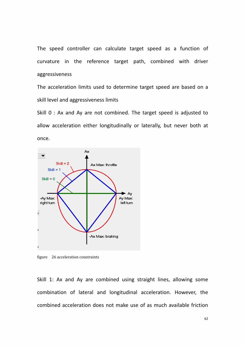
The speed controller can calculate target speed as a function of
curvature in the reference target path, combined with driver
aggressiveness
The acceleration limits used to determine target speed are based on a
skill level and aggressiveness limits
Skill 0 : Ax and Ay are not combined. The target speed is adjusted to
allow acceleration either longitudinally or laterally, but never both at
once.
figure 26 acceleration constraints
Skill 1: Ax and Ay are combined using straight lines, allowing some
combination of lateral and longitudinal acceleration. However, the
combined acceleration does not make use of as much available friction

63
as is used in pure longitudinal or pure lateral acceleration.
Skill 2: Ax and Ay are combined using a friction ellipse, providing a
consistent use of available friction regardless of the direction of the total
acceleration vector.
After that talking about the path preview length set the data as same as
camera configuration and characteristic of lane detection function.
Previewing of the target path is configured with four length parameters
1.Arc length used to estimate curvature: Length of path segment used to
calculate curvature at the mid-point of the segment
2. Preview start :The portion of the reference path that is previewed
figure 27 preview length
64
starts this distance in front of the origin of the vehicle sprung mass
coordinate system (typically the origin is at the center of the front axle)
3. Total preview: This defines the portion of the reference path that is
previewed. Longer distances sometimes give better results for
complicated paths combined with aggressive acceleration settings.
4. Preview interval: Interval for calculating path curvature and target
speed over the preview path
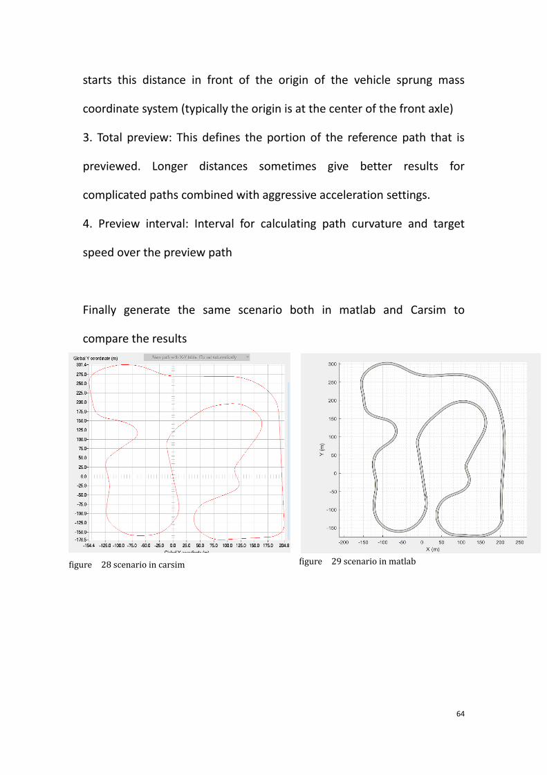
Finally generate the same scenario both in matlab and Carsim to
compare the results
figure 29 scenario in matlab
figure 28 scenario in carsim
65
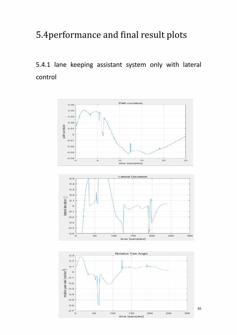
5.4performance and final result plots
5.4.1 lane keeping assistant system only with lateral
control

66
From figure 30, the results of controller are presented such as
curvature, lateral deviation, relative yaw angle, steering angle and driver
path of autonomous car. In the driver path plot the blue line represents
center line of two boundaries the red line is path of vehicle.
The controller performance is good enough to achieve lane keeping
requirement. The steering angle is in the range of [-0.2 +0.3] rad.
figure 30 performance plot A
67
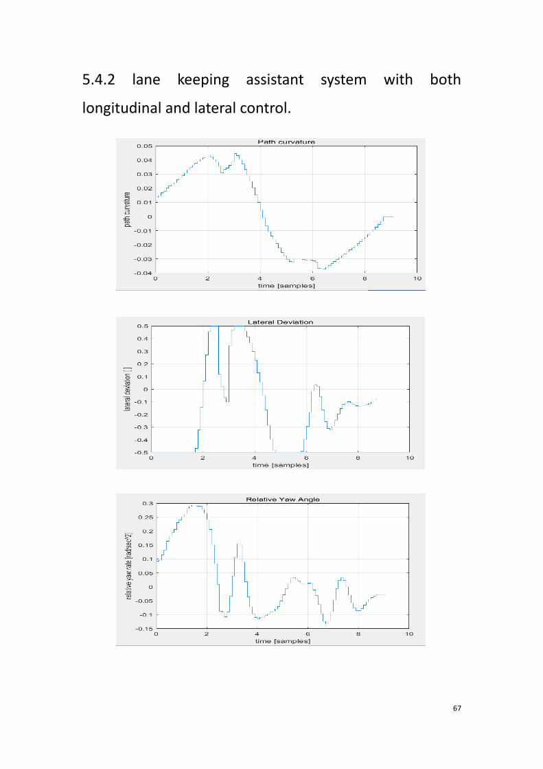
5.4.2 lane keeping assistant system with both
longitudinal and lateral control.

68

69
Apart from items introduced before here the acceleration command
and longitudinal velocity are included. Based on the curvature the
reference velocity is calculated and autonomous driving car follows it.
Since the velocity is not constant as before when cross curvature the
speed is higher than before. As the result of it the steering angle is in the
range of [-0.4 +0.5]
figure 31 performance plot B

70
5.4.3 benchmarking with Carsim
Speed comparison
Steering angle comparison
G-G plot comparison

71
G-G plot, which represents the time history of longitudinal and lateral
acceleration, is a main indicator of formula racing car. Here the results of
2 software is quiet same.
Due to the reason of software default set in Carsim the speed profile is
starting from speed limit which is 80 km/h since in matlab it starts from
0km/h. For the steering angle matlab has smoother maneuver than
Carsim.
figure 32 benchmarking reslts comparision
Vehicle path comparison

72
Reference
1 .F. K¨uhne, “Model Predictive Control of a Mobile Robot Using linearization,” APS/ECM,
2.R. C. Rafaila, “Nonlinear Model Predictive Control of Autonomous vehicle Steering,” 2015 19th
International Conference on System Theory, Control and Computing (ICSTCC), October 14-16, Cheile
Gradistei, Romania
3.M.Brown, “Safe driving envelopes for path tracking in autonomous vehicles,” Control
EngineeringPractice61 (2017)307–316
4.J. Y. Goh, “Simultaneous Stabilization and Tracking of Basic Automobile Drifting trajectories,” 2016
IEEE Intelligent Vehicles Symposium (IV) Gothenburg, Sweden, June 19-22, 2016
5.Jiechao Liu, “THE ROLE OF MODEL FIDELITY IN MODEL PREDICTIVE CONTROL BASED HAZARD
VOIDANCE IN UNMANNED GROUND VEHICLES USING LIDAR SENSORS,” Mechanical Engineering,
University of Michigan, Ann Arbor,Mi,48109
6 .S. C. Peters, “Differential flatness of a front-steered vehicle with tire force control,”2011 IEEE/RSJ
International Conference on intelligent Robots and Systems September 25-30, 2011. San Francisco,
CA, USA
7.R. Skjetne, “Robust output maneuvering for a class of nonlinear systems,” Automatic, vol. 40, no.
3, pp.373–383, 2004.
8.P. Aguiar, “Logic-based switching control for trajectory-tracking and path-following of
underactuated autonomous vehicles its parametric modeling uncertainty,” presented at the 2004
Amer.Control Conf., Boston, MA, Jun. 2004.
9.S. Al-Hiddabi, “Tracking and maneuver regulation control for nonlinear nonminimum phase
systems: Application to flight control,” IEEE Trans. Control Syst. Technol., vol. 10, no. 6, pp.
780–792,Jun. 2002.
10.A. P. Aguiar, “Path following reference-tracking? An answer relaxing the limits to performance,”
5th IFAC/EURON Symp. Intelligent AutonomousVehicles, Lisbon, Portugal, Jul. 2004.
11.Vincent A. Laurense, “Path-Tracking for Autonomous Vehicles at the Limit of Friction,” 2017
American Control Conference May 24–26, 2017, Seattle, USA
12.C. I. Chatzikomis, “A path-following driver model with longitudinal and lateral control of vehicle’s
motion,” Forsch Ingenieurwes (2009) 73: 257–266
13.MacAdam CC, “Understanding and modeling the human driver,” Vehicle System Dynamic
40:101–134
14 .Plochl .M, “Driver models in automobile dynamics application.” Vehicle System Dynamic
45:699–741
15. R.Marino, “ A Nested PID Steering Control for Lane Keeping in Vision Based Autonomous
Vehicles,” 2009 American Control Conference Hyatt Regency Riverfront, St. Louis, MO, USA June
10-12, 2009
16. C.M. Kang, “Comparative Evaluation of Dynamic and Kinematic Vehicle Models,’’53rd IEEE
Conference on Decision and Control December 15-17, 2014. Los Angeles, California, USA
17.A. Eskandarian, “ Handbook of Intelligent Vehicle,” Spriger-Verlag,2012.

73
18 .A. G. Ulsoy, “Automotive Control Systems,” Cambridge, 2012.
19.S.-H. Lee, “Multirate active steering control for autonomous vehicle lateral maneuvering,” in
Proceeding of IEEE Intelligent Vehicles Symposium, pp. 772-777, June 3-7, 2012.
20.J. H. Lee, “Predictive control of vehicle trajectory by using a coupled vector with the vehicle
velocity and sideslip angle,” accepted to IJAT (2008).
21.D.Gu, “Neural predictive control for a carlike mobile robot,” Robotics and Autonomous Systems
39 (2) (2002) 73-86.
22 H.B. Pacejka, “Tire and Vehicle Dynamics”. Elsevier – Butterworth Heinemann, 2004.
23.N. D. Smith, “ Understanding Parameters Influencing Tire Modeling,” Colorado State University,
(2004) Formula SAE Platform
24. Sharp RS et al., “A mathematical model for driver steering control, with design, tuning and
performance results.” Vehicle Sys Dynamic 33:289–326
25.T.Stanger,“A Model Predictive Cooperative Adaptive Cruise Control Approach.”. 2013 American
Control Conference (ACC) Washington, DC, USA, June 17-19, 2013