copyright by tan wang 2014

Copyright

by

Tan Wang

2014

The Thesis Committee for Tan Wang

Certifies that this is the approved version of the following thesis:

Solving Dynamic Repositioning Problem for Bicycle Sharing Systems:

Model, Heuristics, and Decomposition

APPROVED BY

SUPERVISING COMMITTEE:

Chandra R. Bhat

Stephen D. Boyles

Supervisor:



by

Tan Wang, B.E.

Thesis

Presented to the Faculty of the Graduate School of

The University of Texas at Austin

in Partial Fulfillment

of the Requirements

for the Degree of

Master of Science in Engineering

The University of Texas at Austin

December 2014

Dedication

To my parents.

v

Acknowledgements

I would like to thank all the people who made this thesis possible. First of all, I

would like to express my great appreciation to my supervisor, Dr. Chandra Bhat. His

insightful guidance, strict training and substantial support inspired, ignited and excited me

to move forward through my graduate study. Also, his expertise in and passion for the

transportation field encouraged me to make a decision of going further on the way of

research. Then I am especially grateful for Dr. Stephen Boyles, the second reader of my

thesis, for his immediate feedback and useful suggestions on this thesis. He is always

approachable to answer my questions. I learned quite a bit about how to make a better

structure of papers from his valuable comments.

I would like to thank Capital Bikeshare for sharing their system data online.

I also would like to express my thanks to my dear friends for their help and

encouragement, which is supportive enough when I was mired in the research process.

Last but not least, I would like to offer my sincere thanks to my parents, who offered

endless love and support to me. I so appreciate everything they have done for me.

vi

Abstract



Tan Wang, M.S.E.

The University of Texas at Austin, 2014

Supervisor: Chandra R. Bhat

Bicycle sharing systems (BSS) have emerged as a powerful stimulus to non-

motorized travel, especially for short-distance trips. However, the imbalances in the

distribution of bicycles in BSS are widely observed. It is thus necessary to reposition

bicycles to reduce the unmet demand due to such imbalances as much as possible. This

paper formulates a new mixed-integer linear programming model considering the dynamic

nature of the demand to solve the repositioning problem, which is later validated by an

illustrative example. Due to the NP-Hard nature of this problem, we seek for two heuristics

(greedy algorithm and rolling horizon approach) and one exact solution method (Benders’

decomposition) to get an acceptable solution for problems with large instances within a

reasonable computation time. We create four datasets based on real world data with 12, 24,

36, and 48 stations respectively. Computational results show that our model and solution

methods performed well. Finally, this paper gives some suggestions on extensions or

modifications that might be added to our work in the future.

vii

Table of Contents

List of Tables ......................................................................................................... ix

List of Figures ..........................................................................................................x

CHAPTER 1 INTRODUCTION .............................................................................1

1.1 Literature Review......................................................................................1

1.2 Motivation .................................................................................................5

1.3 Thesis Outline ...........................................................................................8

CHAPTER 2 PROBLEM DEFINITION .................................................................9

CHAPTER 3 MIXED-INTEGER LINEAR PROGRAMMING MODEL ...........11

3.1 Notation...................................................................................................11

3.2 Formulation .............................................................................................12

CHAPTER 4 ILLUSTRATIVE EXAMPLE .........................................................15

4.1 Input Data................................................................................................15

4.2 Output Results .........................................................................................16

CHAPTER 5 SOLUTION METHODS .................................................................20

5.1 Greedy Algorithm ...................................................................................20

5.2 Rolling Horizon Approach ......................................................................21

5.3 Benders’ Decomposition .........................................................................22

CHAPTER 6 NUMERICAL EXPERIMENTS .....................................................26

6.1 Data Pre-treatment ..................................................................................26

6.2 Computational Results ............................................................................27

6.2.1 Using Greedy Algorithm.............................................................27

6.2.2 Using Rolling Horizon Approach ...............................................29

6.2.3 Using Benders’ Decomposition ..................................................32

CHAPTER 7 CONCLUSIONS AND FUTURE RESEARCH .............................35

7.1 Conclusions .............................................................................................35

7.2 Future Research ......................................................................................36

viii

REFERENCES ......................................................................................................39

ix

List of Tables

Table 1. Travel Time Matrix (in Seconds).............................................................15

Table 2. Discretized Travel Time Matrix (Interval = 300s) ..................................15

Table 3. Initial Inventory and Capacity of Stations ...............................................16

Table 4. Demand Pattern at Each Time Period ......................................................16

Table 5. Optimal Route and Number of Bikes Carried on Vehicle .......................17

Table 6. Total Unmet Demand after Repositioning ...............................................18

Table 7. Optimal Solution Using GA with T = 5 ...............................................27

Table 8. Optimal Solution Using GA with T = 10 .............................................28

Table 9. Optimal Solution Using RHA with 𝛿= 1 ................................................30

Table 10. Optimal Solution Using RHA with 𝛿= 2 ..............................................30




Table 14. Optimal Solution Using Benders’ Decomposition ................................33

x

List of Figures

Figure 1. Trips to/from Columbus Circle/Union Station .........................................6

Figure 2. Number of Full/Empty Instances in Capital Bikeshare System ...............7

Figure 3. Inventory Level at Each Time Period ( = 900) ..................................19

Figure 4. Inventory Level at Each Time Period ( = 100) ..................................19

Figure 5. Rolling Horizon Approach .....................................................................21

Figure 6. Comparison of Different 𝛿 ....................................................................32

Figure 7. Comparison of Obj. Value ......................................................................34

Figure 8. Comparison of Computation Time .........................................................34

1

CHAPTER 1 INTRODUCTION

1.1 LITERATURE REVIEW

Climate change and the energy crisis have triggered a great amount of research on

sustainable development in recent decades. The most widely used definition of sustainable

development is from the World Commission on Environment and Development (WCED):

Sustainable development is development that meets the needs of the present without

compromising the ability of future generations to meet their own needs (see WCED, 1987).

As an essential component of socio-economic activities, transportation systems also need

to incorporate the concept of sustainability to best serve current and future users.

Although there is no standard definition of transportation sustainability, Black et

al. (2002) summarized the objectives and attributes of a sustainable transportation system

based on literature reviewed. Most previous works focused on satisfying the requirements

for a sustainable environment, such as minimizing fossil fuel depletion, greenhouse gas

emissions, and noise pollution. However, the objectives of a sustainable transportation

system involve more than environmental sustainability. Economic developments and

socio-cultural issues should be also considered. Jeon and Amekudzi (2005) characterized

the indicators and metrics of transportation sustainability, classifying them into four

categories: transportation (including safety), economic, environmental, and socio-

cultural/equity. Litman (2007) also studied the indicators for transportation sustainability

but placed more emphasis on the role of indicators in sustainable transportation planning,

which is a feasible approach to realizing transportation sustainability. Black (2010)

provided another set of indicators to consider in achieving a sustainable transportation

2

system: pricing, policy, education, and technology. Pricing and taxation could be treated

as a special policy to manage travel demand in a sustainable way. This approach has already

resulted in great achievements in major cities like London and Singapore.

The emerging field of Intelligent Transportation Systems (ITS) is growing in

response to developments in telecommunications technology. While ITS concepts were

first broached in the 1930s, ITS is only now in its product development period (see

Figueiredo et al., 2001). The principal motivation for building ITS networks is to enhance

traffic and safety management by creating communication pathways between vehicles and

transportation infrastructures (see Dimitrakopoulos and Demestichas, 2010).

Non-motorized travel modes, such as walking and cycling, contribute to a

sustainable transportation system. Transportation researchers in recent years have

encouraged these modes for their environmentally friendly nature. These modes can

provide many benefits to users and the community at large by improving public fitness and

health, providing a cost savings for consumers, and reducing traffic congestion, road and

parking facility costs, total accident risk, energy consumption, and pollution emissions (see

Litman, 2010). Recently, bicycle sharing systems (BSS) have emerged as a powerful

stimulus to non-motorized travel, especially for short-distance trips. A survey shows that

bicycle sharing has positive influence on reducing automobile and taxi usage, and

increasing bicycling and walking (see Shaheen et at., 2013).

BSS has passed through three generations and now is going into its fourth

generation (see Shaheen et al., 2011). The first BSS was launched in Amsterdam in 1965

with all fifty bicycles permanently unlocked, resulting in theft of and damage to the fleet.

To improve this situation, the second generation of BSS, based on a coin-deposit system,

first appeared in Copenhagen in 1995. However, there were still problems with theft and

damage under the coin-deposit system because the users were anonymous. Incorporating

3

advanced information technologies, the third generation BSS, known as the Vélo a la Carte

System, appeared in Rennes, France in 1998 (see Midgley, 2011). The electronically

locking and identification mechanism effectively avoid the problem that the second

generation BSS had. This approach to a BSS met with great success and rapidly spread.

This BSS is now established in over 165 cities around the world, such as the Vélib’ system

in Paris, Capital Bikeshare in Washington D.C., and Hangzhou Public Bicycle. The three

main components are bicycles, stations, and operating centers. Bicycles are made

accessible to the public in specific docking stations, where users can pick up and return

bicycles with a membership card. To encourage people to use the system, some BSS (such

as Capital Bikeshare) use a pricing scheme that provides the first 30 minutes free. Realizing

that a BSS is not only an independent system but a part of sustainable transportation

system, researchers have begun to consider the connectivity of BSS to other travel modes,

especially to existing public transit systems, which leads the way to the fourth generation

of BSS.

Lin and Yang (2011) addressed the design of the BSS and formulated the strategic

planning problem as a non-linear mixed integer programming problem. Their approach

becomes intractable when solving the real-world problem because of the nonlinearity and

complexity of the formulation. Shu et al. (2010) also developed a deterministic linear

programming model to support decision-making in the design and management of BSS.

Vogel and Mattfeld (2011) used data mining to explore the activity patterns in BSS,

noting the imbalances in the distribution of bicycles. For instance, users tend to pick up

bicycles from stations located higher on a hill and return them in stations located downhill.

As a result, no bicycles are available in hilltop stations and no vacant docks are available

in stations downhill if the operators do not take action. Due to the imbalance of demand

and supply at each station, the BSS operators need to redistribute the bicycles in order to

4

optimize the system performance. In other words, redistribution (i.e., repositioning) is

critical for the BSS to meet the demand for bicycles at the origin stations and vacant docks

in the destination stations. Usually a fleet of trucks is used to transfer bicycles among

stations during a specific time period. The problem of finding an optimal repositioning

route and determining the number of bicycles to transfer while the demand for bicycles is

negligible, e.g., in the evening, is referred to as a static repositioning problem (SRP);

similarly, optimizing the redistribution route while the demand is high, e.g., during the day,

is referred to as a dynamic repositioning problem (DRP).

Many researchers have made great contributions to modeling and solving this

particular SRP in recent years. One intuitive approach is to model it based on the well-

known Traveling Salesman Problem (TSP) (see Miller et al., 1960) with pickup and

delivery (see Hernández-Pérez et al., 2004). Benchimol et al. (2011) adapted a 9.5-

approximation algorithm for C-delivery TSP (see Chalasani and Motwani, 1999) to solve

their SRP model, whose objective is to achieve a given target bicycle inventory level for

each station at the end of the repositioning action, allowing no deviations. However, the

method used to determine the target was not clearly stated. Erdogan et al. (2012) relaxed

the objective by allowing the target inventory level for each station to fall within a range.

However, the criterion for determining the lower bounds and upper bounds was not

specified. Raviv et al. (2013) extended the one-commodity pickup and delivery TSP for

the SRP. One of the ingenious extensions is that they introduced a convex penalty function

as a part of the objective function. The penalty function was suggested to represent the

expected amount of shortages at a station. In order to calculate the expectation value, they

modeled the dynamics of the bicycles inventory level as a continuous-time Markov chain—

more specifically, a non-homogenous Poisson process. Rainer-Harbach et al. (2013)

presented a Variable Neighborhood Search metaheuristic with an embedded Variable

5

Neighborhood Descent, for solving the BSS inventory distribution problem. However, they

did not mention how the target number of available bikes after repositioning is determined.

In response to the advancement made on the SRP, some researchers turned to the

DRP. Contardo et al. (2012) used Dantzig-Wolfe decomposition (see Dantzig and Wolfe,

1960) and Benders’ decomposition (see Benders, 1962) to solve the DRP, but the demand

pattern they used was set by a formula that might not be realistic enough. Benarbia et al.

(2013) introduced a new approach based on Petri nets with variable arc weights to model

the DRP. However, this model was only tested by simulations, and its application to a real-

world BSS was not specified. Caggiani and Ottomanelli (2013) also provided a simulation

model for DRP. Schuijbroek et al. (2013) proposed a new cluster-first route-second

heuristic to solve DRP. One special feature in their model is the service level requirements

at each station, which use the proportion of expected value of total satisfied demand and

expected value of total demand. Nair et al. (2013) used a stochastic characterization of

demand and a model developed in their prior work, in which they employed fleet-

management strategies to deal with DRP.

1.2 MOTIVATION

This paper is primarily concerned with dynamic repositioning since it directly

balances the number of bicycles and vacant lockers in a BSS, especially during the peak

hours. Note that the peak hours for a BSS might differ from that of motorized vehicles.

Working with the trip history data of Capital Bikeshare System in Washington

D.C., we observed a very high rate usage at some stations in certain months. For example,

Figure 1 shows the number of trips to and from the Columbus Circle/Union station during

the last 12 months. Nearly 7000 departures and 6700 arrivals occurred at this station during

September 2013.

6

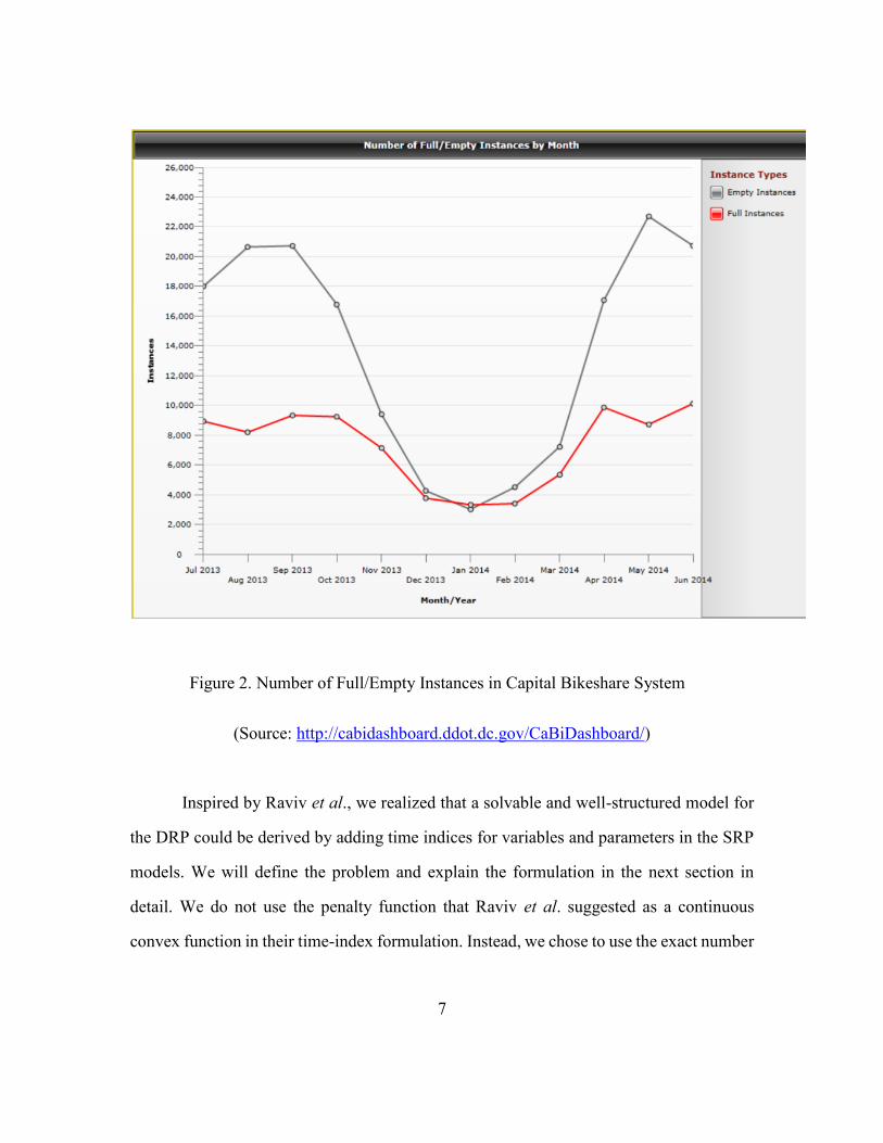
(Source: http://cabidashboard.ddot.dc.gov/CaBiDashboard/)

Figure 2 clearly reveals the serious imbalances in Capital Bikeshare’s inventory

flow. Completely full or completely empty stations discourage users. A strategic static

repositioning action at night may alleviate the imbalance only at the beginning of the next

day, but will not address imbalances that arise during the peak daytime hours. Thus, for a

high-usage BSS, a dynamic repositioning action in the daytime is also needed.

Figure 1. Trips to/from Columbus Circle/Union Station

http://cabidashboard.ddot.dc.gov/CaBiDashboard/

7

(Source: http://cabidashboard.ddot.dc.gov/CaBiDashboard/)

Inspired by Raviv et al., we realized that a solvable and well-structured model for

the DRP could be derived by adding time indices for variables and parameters in the SRP

models. We will define the problem and explain the formulation in the next section in

detail. We do not use the penalty function that Raviv et al. suggested as a continuous

convex function in their time-index formulation. Instead, we chose to use the exact number

Figure 2. Number of Full/Empty Instances in Capital Bikeshare System

http://cabidashboard.ddot.dc.gov/CaBiDashboard/

8

of shortages based on the historic data during a given time period. Thus, we assume that

the forecasting demand is the same as the real-world demand.

By employing discretization of the time, we can formulate the DRP as an Integer

Programming (IP) problem, which has been well studied and can be solved by many

developed solvers, such as the CPLEX optimization software package.

1.3 THESIS OUTLINE

The rest of this thesis is structured as follows.

Chapter 2 provides a formal definition of the essential problem in this thesis.

Chapter 3 explains each component of our model, from notations to the

interpretations of objective function and constraints.

Chapter 4 validates the rationality of our model by solving an illustrative example.

Chapter 5 presents three different solution methods for solving large instances

problem efficiently. Two of them are heuristics-based, and the third is based on Benders’

decomposition.

Chapter 6 describes the real-world data used in this thesis and shows computational

results of using each solution method described in Chapter 5.

Chapter 7 summarizes this thesis and discusses several future works that might be

extended from this thesis.

9

CHAPTER 2 PROBLEM DEFINITION

Suppose we are given a complete digraph ( , ) , where the set of nodes

{0,1, , }n includes a depot indexed with 0 and all stations in the BSS. A

repositioning vehicle travels from the depot to visit all stations and transport desired

number of bicycles at each station. Each station is given a capacity (number of docks) and

an inventory level (number of bicycles and thus number of vacant docks). Each arc

( , )i j is associated with a travel cost. We are also given the expected (forecasting)

demand for bicycles and vacant docks at each station. We have two objectives for this

problem. One is to decrease the total unmet demand for both vacant docks and bicycles as

much as possible. The other is to minimize the total travel cost for the repositioning vehicle.

We measure the unmet demand as the non-negative difference between the

expected demand and the current inventory level for all stations. In this paper we do not

assume the dynamics of demand as a specific stochastic process as some researchers

did,since it would introduce a more complicated problem on estimating the parameters of

such stochastic process. Notice that the quality of the demand forecast would affect the

effectiveness of the repositioning decision. However, in our model (presented in Chapter

3) the demand forecast is just a given input, so the quality of the demand forecast would

not affect the performance of our model in terms of computational time. In other words,

we are considering a repositioning problem in which the demand forecast is given.

Computational time matters in our problem because the repositioning action might be

needed for several times within a short timeframe in some busy BSS. In order to conduct

the numerical experiments (described in Chapter 6), we assume that the demand forecast

is the same as that in reality, which means the demand forecast is 100% accurate. To apply

10

our model in real-world projects, an associated demand forecast model should be

developed as well, which is not in the scope of this thesis.

It is obvious that the repositioning problem involves with the well-studied vehicle

routing problem. We need to determine the number of bicycles to load or unload at each

station while finding an optimal repositioning route.

Unlike the classic TSP we are allowing the repositioning vehicle to visit a station

more than once. More visits on a station can decrease the unmet demand but increase the

travel cost. This trade-off process might result in a better solution than imposing the

constraint of number of visits at a station.

Since we discretize time and all the variables in this problem are integers, we will

present a new Integer Linear Programming (ILP) formulation under assumptions

mentioned above.

The input data for this problem is as follows.

1) Initial inventory (number of bicycles) and capacity (total number of docks) of

each station.

2) Travel times between stations.

3) Demand for both bicycles and vacant docks at each station in each time period.

The output for this problem is a route for the repositioning vehicle during the whole

action and number of bicycles to be loaded and unloaded at each station.

11

CHAPTER 3 MIXED-INTEGER LINEAR PROGRAMMING MODEL

3.1 NOTATION

Sets

Set of stations with a depot indexed by 0.

Set of time periods. Let /M T .

Parameters

0

is Initial inventory level of station i.

ic Capacity of station i.

Time period length (interval).

ijt Travel time from station i to station j.

ijm Number of time periods from station i to station j. /ijij tm .

T Total repositioning time.

,

P

i td Demand for bicycles at station i during tth period.

,

R

i td Demand for vacant docks at station i during tth period.

C Capacity of the repositioning vehicle.

Decision Variables

,ij tx Binary, equal to 1 if the vehicle travels from station i to station j during tth period.

,ij tn Number of bicycles carried on the vehicle when traveling from station i to station

j during tth period.

,i ty Number of bicycles loaded onto the vehicle at station i during tth period.

,i tl Number of unsatisfied docks at station i during tth period.

,i tb Number of unsatisfied bicycles at station i during tth period.

,i ts Number of bicycles at station i during tth period.

12

3.2 FORMULATION

The objective function is to minimize total travel cost and total unmet demand

during the whole repositioning process. In this paper we just use travel time as a measure

of travel cost. Since this problem includes multiple objectives, we need to introduce a

weight that indicates the importance of each objective. This weight also has a specific

meaning, namely one additional unmet demand is equivalent to seconds of additional

travel time in this case.

, , ,minimize ( )ij ij t i t i t

i j t i t

t x l b

First we consider the constraints which represent the balance of inventory level at

each station during each period.

, , 1 , , , , , ,,R P

i t i t i t i t i t i t i ts s y d d l b i t

Note that we do not define time period 0, so it will cause an error when t = 1 for

these constrains since we have a subscript of t-1. To avoid such problems, we can simply

add another constraints 0

,0 ,i is s i or use if-then-else type conditional

constraints when programming.

Next we write constraints for unsatisfied demand for bicycles and docks

respectively. By the definition of unsatisfied demand, it is quite straightforward to write as

the form of , , , 1[ ]R

i t i t i i tl d c s

, , , , 1[ ]P

i t i t i tb d s

, where the notation max[ ] { ,: 0}x x

. However, these equality constraints are nonlinear constraints, which would make our

problem more intractable. Fortunately, this issue is easy to fix in the following way.

, , , , 1, ,R P

i t i t i t i i tl d d c s i t

, , , , 1, ,P R

i t i t i t i tb d d s i t

, integers0, , ,i tl i t

13

, integers0, , ,i tb i t

Since we are considering a minimizing problem, the above constraints can actually

guarantee the number of unsatisfied lockers ,i tl and unsatisfied bicycles ,i tb take the

right value in an optimal solution.

Like classic vehicle routing problem, we need constraints describing the movement

of the repositioning vehicle. The first rule is that it starts from the depot and returns at

the end of reposition action.

0 ,1 1j

j

x

, 00, 1

jj M m

j

x

Then we have flow conservation condition, i.e. the repositioning vehicle can only

leave from a node which it just entered.

, , , , \{1, }jiji t m ik t

j k

x x i t M

Note that for some t, the subscript jit m might be non-positive. To solve this

problem, one way is to set those x’s equal to zero, but this requires more memory space to

create a larger time index set . Another way is to add a condition for that subscript:

, , , , \{1, } s.t. 0jiji t m ik t ji

j k

x x i t M t m

We suggest this modification because it not only avoids the problem when

implementing in program but also reduces the number of constraints.

The repositioning vehicle can only appear on one particular link in a given time

period.

, 1,ij t

i j

x t

Note that we assume , 0ij tx if period t is not the first period when the

repositioning vehicle moving from station i to j, otherwise the first part of our objective

14

function cannot represent the total travel time. That’s why we use less than and equal to

sign in these constraints.

We also should have a balance constraint on bicycles to insure there is no missing

bicycle during the loading and unloading process.

, , , , , \{1, } s.t. 0jiji t m ik t i t ji

j k

n n y i t M t m

The number of bicycles the repositioning vehicle can carry, ,ij tn , cannot excess

the vehicle capacity, and it should be zero when the repositioning vehicle is not traveling

from station i to j at time period t.

, , , , ,ij t ij tn C x i j t

We need to avoid the situation that bicycles in some node are loaded or unloaded

in a period even the node is not visited by the vehicle.

, , , ,i t i ij t

j

y c x i t

, , , ,i t i ij t

j

y c x i t

At last, we need non-negativity and integrality constraints.

, integers , ,i ty i t

, integers0, , , ,ij tn i j t

, integers0 , , ,i t is c i t

, {0,1}, , ,ij tx i j t

15

CHAPTER 4 ILLUSTRATIVE EXAMPLE

In this chapter we use a simple example to illustrate our model, focusing only on

the inputs and outputs of the model. For a large instance problem, it is intractable to solve

directly even using a highly efficient solver. We will present several solution methods in

the next chapter.

4.1 INPUT DATA

Table 1. Travel Time Matrix (in Seconds)

Station 0 1 2 3 4

0 0 600 900 600 900

1 600 0 600 900 600

2 600 900 0 300 600

3 900 300 300 0 600

4 600 900 600 600 0

Table 1 gives travel times between 5 stations. Note that the depot is indexed by 0.

Table 2. Discretized Travel Time Matrix (Interval = 300s)

Station 0 1 2 3 4

0 1 2 3 2 3

1 2 1 2 3 2

2 2 3 1 1 2

3 3 1 1 1 2

4 2 3 2 2 1

16

Table 2 provides number of time periods between 5 stations. We set 1iim to

allow the repositioning vehicle to stay more than one time period on some stations if

necessary.

Table 3. Initial Inventory and Capacity of Stations

Station Initial Inventory Capacity

1 12 15

2 12 18

3 10 20

4 9 15

Table 3 gives the initial inventory and capacity of stations. We do not set constraints

on the inventory level and capacity of the depot.

Table 4. Demand Pattern at Each Time Period

Station 1 2 3 4

Demand (Bikes, Lockers) (6, 7) (5, 6) (9, 7) (5, 5)

In this example, we assume that the demand pattern is time-homogenous, namely

the demand for bicycles and vacant lockers keeps the same at each time period. See Table

4.

We set the capacity of repositioning vehicle as 20. The total repositioning time is

fixed to 2.5 hours (9000s).

4.2 OUTPUT RESULTS

We solved this problem using IBM-ILOG CPLEX 12.6 on an Intel Core i5 2.6 GHz

with 8GB of RAM.

17

Table 5. Optimal Route and Number of Bikes Carried on Vehicle

Time Period = 900 = 100

Route Bikes Carried Route Bikes Carried

1 (0, 3) 10 (0, 3) 11

2

3 (3, 1) 0 (3, 1) 0

4 (1, 2) 11 (1, 1) 1

5 (1, 2) 16

6 (2, 2) 20

7 (2, 2) 13 (2, 2) 17

8 (2, 3) 20 (2, 2) 18

9 (3, 3) 2 (2, 3) 20

10 (3, 1) 0 (3, 2) 1

11 (1, 4) 11 (2, 2) 19

12 (2, 3) 20

13 (4, 2) 5 (3, 3) 14

14 (3, 3) 12

15 (2, 3) 20 (3, 3) 20

16 (3, 3) 8 (3, 3) 8

17 (3, 3) 6 (3, 3) 20

18 (3, 3) 4 (3, 3) 20

19 (3, 3) 2 (3, 3) 2

20 (3, 1) 0 (3, 1) 0

21 (1, 0) 4 (1, 1) 1

22 (1, 1) 2

23 (0, 0) 4 (1, 1) 3

24 (0, 0) 4 (1, 1) 4

25 (0, 0) 4 (1, 1) 19

26 (0, 0) 4 (1, 1) 20

27 (0, 0) 4 (1, 0) 9

28 (0, 0) 4

29 (0, 0) 4 (0, 0) 9

30 (0, 0) 4 (0, 0) 9

18

Table 6. Total Unmet Demand after Repositioning

Unmet Demand = 900 = 100

Bikes 0 0

Lockers 1 3

As we mentioned in the previous section, measures the relative importance

between unmet demand and travel time. A smaller will force the repositioning vehicle

to consider more on saving travel time. We can see from Table 5 that when = 100 the

repositioning vehicle chose to stay at station 3 from period 13-19 and stay at station 1 from

period 21-26. As a result, the total unmet demand with a smaller is greater because

saving travel time is more important than minimizing the unmet demand. This could be

seen in Table 6.

Note that the demand for bicycles and lockers in station 4 is intentionally set to be

self-balanced. It is natural for the repositioning vehicle to not consider visiting station 4;

however, since it has a limited capacity, the repositioning vehicle has a nonzero probability

of visiting station 4 to unload some bikes in order to increase the capability of carrying

bicycles between station 1, 2, and 3.

We also provide dynamic inventory level of each stations during the repositioning

process. Please see Figure 3 ( = 900) and Figure 4 ( = 100).

19

Figure 3. Inventory Level at Each Time Period ( = 900)

Figure 4. Inventory Level at Each Time Period ( = 100)

0

5

10

15

20

25

1 2 3 4 5 6 7 8 9 1 0 1 1 1 2 1 3 1 4 1 5 1 6 1 7 1 8 1 9 2 0 2 1 2 2 2 3 2 4 2 5 2 6 2 7 2 8 2 9 3 0

NU

MN

ER O

F B

IKES

IN S

TATI

ON

TIME PERIOD

Station 1 Station 2 Station 3 Station 4

0

5

10

15

20

25

1 2 3 4 5 6 7 8 9 1 0 1 1 1 2 1 3 1 4 1 5 1 6 1 7 1 8 1 9 2 0 2 1 2 2 2 3 2 4 2 5 2 6 2 7 2 8 2 9 3 0

NU

MB

ER O

F B

IKES

IN S

TATI

ON

TIME PERIOD

Station 1 Station 2 Station 3 Station 4

20

CHAPTER 5 SOLUTION METHODS

Because of the NP-Hard (non-deterministic polynomial-time hard) nature of this

problem, we need to seek more efficient methods to solve for larger instances problem.

First we will provide two heuristics which are computational efficient and might provide a

near-optimal solution: Greedy Algorithm and Rolling Horizon Approach. Then we will

apply Benders’ Decomposition technique to solving this problem in an exact algorithmic

framework.

5.1 GREEDY ALGORITHM

Greedy algorithm is one of the most commonly used heuristic in order to reduce

the problem size. Usually the original problem is divided by time index into several stages

or sub-problems. Greedy algorithm is just to find the locally optimal solution at each stage

with the hope of finding globally optimal solution at the last stage. For example, in our

problem applying greedy algorithm is to tell the repositioning vehicle to stay at the station

where it currently is unless there will be a large unmet demand at some other station at next

planning stage. We denote the length of planning stage as T .

We describe the process of greedy algorithm as follows.

ALGORITHM

Initialize t = 1.

DO WHILE t M

Solve problem within time window [ , ]t t T

Fix all variables within time window [ , ]t t T

Let t = t+ T +1

21

END DO

Although greedy algorithm greatly speeds up computations by solving multiple

sub-problems with much smaller problem sizes, it can produce the optimal solution at last

only if the original problem has optimal substructure. In many cases, problems do not have

such structure and thus more sophisticated dynamic programming techniques are need to

find the global optimal solution. Unfortunately, our problem belongs to the one which does

not have optimal substructure. However, we still can apply greedy algorithm to get a

heuristic solution, which could be an upper bound of our (minimizing) problem.

5.2 ROLLING HORIZON APPROACH

It is natural to apply rolling horizon approach for time index based problems. Like

greedy algorithm, rolling horizon approach also divides the problem into several sub-

problems instead of solving the whole problem at once. Each time we only solve the sub-

problem within a planning horizon [ , ]t t T . The most significant difference between

rolling horizon approach and greedy algorithm is that we only fix variables in a smaller

time interval [ , ] [ , ]t t t t T at each iteration. The next iteration should start at

time period 1t with a planning horizon length of T . We illustrate rolling horizon

approach using the following figure.

Figure 5. Rolling Horizon Approach

22

We also describe the process of greedy algorithm as follows.

ALGORITHM

Initialize t = 1.

DO WHILE t M

Solve problem within time window [ , ]t t T

Fix all variables within time window [ , ]t t

Let t = t+ +1

END DO

Rolling horizon approach is also a heuristic for finding globally optimal solution

with hope of achieving it through finding optimal solution of sub-problems successively.

However, unlike greedy algorithm which fixes all variables decided in one sub-problem,

rolling horizon approach relaxes some of decision variables in the current planning horizon,

allowing them entering next planning horizon in order to get better objective value.

5.3 BENDERS’ DECOMPOSITION

Benders’ decomposition is a solution method for solving problems with a special

block ladder structure. The following is an example of such block ladder structure.

(OP) minimize T Tc x g y

s.t.

, 0

Ax b

Dx Fy d

x y

We often denote the second constraint as “complicating” constraint, because it

involves with most (in this case, all) variables of the problem. For the rest constraint, it is

natural to solve them separately for the associated part of objective function. For example,

if we do not consider the complicating constraint, the only thing we need to do is to

minimize objective function Tc x over constraint , 0Ax b x because there’s no y

23

variable in the constraint. Considering the fact that the complicating constraint cannot be

ignored, Benders’ decomposition works as follows: it decomposes the original problem

into a simple so-called master problem and a sub-problem similar to the original one but

without complicating constraints, then it solves these two problems iteratively instead of

solving the original problem with complicating constraints.

We use the above example to illustrate how to construct master and sub-problem in

Benders’ decomposition.

First we assume we already know a feasible solution of variable x, denoted as x0.

The feasibility indicates that 0 { | , 0}x x Ax b x . Then the original problem (OP)

becomes (P1):

0minimize T Tc x g y (P1) minimize gT y

0

0

0

s . t .

, 0

Ax b

Dx Fy d

x y

0s . t .

0

F y d D x

y

We write the dual problem of (P1) as follows:

(DP) 0maximize ( )Tu d Dx

s.t.

0

TF u g

u

Note that we can think the optimal objective function value DPz as a function of

x, denoted as ( )DPz z x . Thus we can write OP as:

(OP1) minimize ( )Tc x z x

s.t.

0

Ax b

x

We call DP as the sub-problem in Benders’ decomposition. In most cases, the sub-

problem has much smaller problem size so that we can solve it directly within reasonable

time. There are two possibilities that would arise when solving the sub-problem: 1) DP is

unbounded above; 2) DP has an optimal solution.

24

In the first case, solving DP will return one of the extreme rays, denoted as *r ,

with the property that

*

0( ) ( ) 0Tr d Dx

This results in

( )z x .

To avoid this situation in the master problem, we need to add a constraint in the

master problem to cut off that specific x0 :

*( ) ( ) 0Tr d Dx

In the second case, solving DP will return one of the extreme points, denoted as *u

, which satisfies

*

0 0( ) ( ) ( )Tz x u d Dx

If we find that x0 is not optimal for the original problem (OP), we can cut off it by

adding a constraint to the master problem:

*( ) ( )Tz u d Dx

Now we can write our master problem as

(MP) minimize Tc x z

*

*

s . t .

0

( ) ( ) 0

( ) ( )

T

T

A x b

x

r d D x

u d D x z

The optimal solution of the master problem (MP) provides a lower bound of the

original problem (OP), while a feasible solution x0 and y0 provide an upper bound of the

OP, 0 0

T Tc x g y . If the difference between upper bound and lower bound is greater than a

threshold, we update the feasible solution x0 with the optimal solution of MP, *x . Then

add new constraints to the master problem based on this updated x0 by solving new

25

associated sub-problem. We terminate this algorithm if the difference between upper bound

and lower bound is small enough.

We describe Benders’ decomposition as follows.

ALGORITHM

Initialize UB = +∞, LB = ∞, 0 { | , 0}x x Ax b x .

DO WHILE UB – LB > ε

Solve sub-problem

0maximize ( )T

uu d Dx

s.t.

0

TF u g

u

IF Unbounded THEN

Get extreme ray *r

Add constraint *( ) ( ) 0Tr d Dx to master problem

ELSE

Get extreme point *u

Add constraint *( ) ( )Tz u d Dx to master problem

UB ← min {UB, *

0 0( ) ( )T Tc x u d Dx }

END IF

Solve master problem

,minimize T

x zc x z

*

*

s.t.

0

( ) ( ) 0

( ) ( )

T

T

Ax b

x

r d Dx

u d Dx z

LB ← * *Tc x z , *

0x x

END DO

26

CHAPTER 6 NUMERICAL EXPERIMENTS

6.1 DATA PRE-TREATMENT

For this study, we used system data recorded on September 26, 2013, by Capital

Bikeshare in Washington D.C., because of the highly active system behavior on that day

(as was indicated in Figure 1). We fixed the total repositioning time to 2.5 hours (9000s),

the same as in the illustrative example. Thus, we used only the data from 14:00 to 16:30

on September 26th, 2013.

As of 2013, there were more than 150 stations in Capital Bikeshare system. To

include all of these stations in our computation would not be wise, since not all of them

necessarily need repositioning. First, some of them might be self-balanced like station 4 in

illustrative example. Second, some of them might be located in a relatively rural area so

that not too many people actually use them. Hence, we chose only stations that satisfy

either of the following conditions:

1) Total demand for bikes and lockers is greater than a threshold (10 in this paper)

during repositioning time;

2) Difference of demand for bikes and lockers is greater than a threshold (5 in this

paper) during repositioning time.

After filtering, we finally got 48 highly active stations. To better understanding how

our solution methods work, we create four groups of data which includes 12, 24, 36, and

48 stations respectively.

Based on the locations of those 48 stations, we calculate the Manhattan distance

matrix. We then assume the average speed of the repositioning vehicle is 1 m/s so that we

can get the travel time matrix.

The initial inventory levels are set to the real levels recorded in our dataset.

27

The capacity of the repositioning vehicle is set to 20 bicycles.

The location of the depot is not clarified through the website of Capital Bikeshare,

so we just select an imaginary place as our depot. We do not set any constraint on the

capacity and initial inventory level of the depot.

We no longer make change of the weight in the objective function in order to

focus on the efficiency of our computation. In this chapter, we set =900.

We apply greedy algorithm and rolling horizon approach using IBM-ILOG CPLEX

12.6 on an Intel Core i5 2.6 GHz with 8GB of RAM. We upload our Benders’

decomposition program to a famous online server, NEOS, to solve our problem.

6.2 COMPUTATIONAL RESULTS

6.2.1 Using Greedy Algorithm

The only parameter we need to specify for applying greedy algorithm (GA) is the

planning length T . In this paper, we set T = 5 and 10 respectively.

We present the computational results in the following tables. All of these problems

achieve optimal solution in a short time.

Table 7. Optimal Solution Using GA with T = 5

Stations Obj. Value CPU Time (s) Travel Time (s) Unmet Demand

12 13920 1.345 1320 14

24 15828 4.043 1428 16

36 29056 15.774 2956 29

48 71189 33.194 2789 76

28

Table 8. Optimal Solution Using GA with T = 10


12 11029 10.269 2029 10

24 18359 85.889 3059 17

36 23097 331.417 3297 22

48 55652 1407.38 4352 57

From Table 7 and Table 8 we can see that with the number of stations increasing,

the optimal objective function value increases simply because larger network expects more

travel time for the repositioning vehicle to reduce the unmet demand as much as possible.

Intuitively we would expect a longer planning length to return us a better solution

in greedy algorithm, since a longer planning length considers more factors in the future;

and thus it would be more likely to give a solution near to the global optimum. We can see

that for the number of stations equal to 12, 36, and 48, the objective function values in

Table 8 are smaller than those in Table 7. Recall that our objective function consists of two

parts, total travel time for the repositioning vehicle and total number of unmet demand

(bicycles and vacant lockers). We can see that in a longer planning algorithm, the

repositioning vehicle takes more time to visit different stations transferring bicycles in

order to meet the demand since the unmet demand has a high weight in the objective

function. However, as we mentioned before, greedy algorithm after all is a heuristic which

cannot guarantee anything. A short planning length no only means “shortsighted” but also

means “flexible” since it fixes much less variables in each iteration. We can see that for

the number of stations equal to 24, the objective function value in Table 7 is smaller than

that in Table 8. It means fixing fewer variables in this case would yield better solution.

29

Computation time is extremely critical especially for those problems which need

immediate responses or decisions. Our repositioning problem in this paper should be

categorized into such problems, because we cannot take a very long computation time, say

several hours, to make a decision for a 2.5-hour action. In practice, we would set a time

limit (3600s or 7200s) to see the best solution that specific algorithm could find out. But in

this problem, we are lucky to find the optimal solution within that time limit. Note that this

“optimal” is under greedy algorithm, probably not the real global optimal solution.

6.2.2 Using Rolling Horizon Approach

Except for the planning horizon length T , we also need to specify the fixing

interval length 𝛿 . The planning horizon length T determines the runtime for each

iteration (roll), and the fixing interval length 𝛿 actually determines the number of

iterations (rolls) until we find out the optimal solution. Based on the experiments on greedy

algorithm, we could estimate the runtime before we actually use rolling horizon approach

to solve our problems. For example, if we choose T = 10 and 𝛿 = 1, we would expect

an approximately 10 times higher CPU time than that in Table 8, since the runtime for each

iteration is the same, but this rolling horizon approach requires 30 iterations while greedy

algorithm only needs 3 iterations. We notice that the CPU time for the problem whose

number of stations is equal to 48 is 1407.38s; we could not bear a 10 times higher runtime

so we decide to fix the planning horizon length T = 5 and change the fixing interval

length from 1 to 5 to see which one would give us a better solution.

We present the results in the following tables.

30

Table 9. Optimal Solution Using RHA with 𝛿= 1


12 10859 4.802 1859 10

24 13450 20.557 4450 10

36 19239 58.814 4839 16

48 56857 167.112 5557 57



12 10320 2.429 1320 10

24 16936 13.265 3436 15

36 22036 30.151 4036 20

48 59289 117.504 4389 61



12 10320 2.11 1320 10

24 17543 8.933 2243 17

36 24795 22.989 4095 23

48 58665 102.589 4665 60

31



12 11220 1.508 1320 11

24 19868 8.035 2768 19

36 24360 27.646 3660 23

48 61565 72.689 3965 64



12 13920 1.297 1320 14

24 15828 4.015 1428 16

36 29056 16.854 2956 29

48 71189 32.403 2789 76

Note that Table 13 should be the same as Table 7 except for the CPU time. We do

not see an obvious relationship between the length of fixing interval given a fixed planning

horizon length and the quality of solution. We present the results in the following figure to

see the relationship more clearly.

32

Figure 6. Comparison of Different 𝛿

From Figure 6 we can see that the best fixing interval length varies for different

number of stations. For number of stations equal to 12, 𝛿=2 or 3 gives best solution; for

number of stations equal to 24, 𝛿=1 gives best solution; for number of stations equal to

36, 𝛿=1 gives best solution; for number of stations equal to 48, 𝛿=1 gives best solution.

Note that the trends of the objective function value are also different. It is an interesting

topic to look into solutions given by heuristics.

6.2.3 Using Benders’ Decomposition

The sub-problem in Benders’ decomposition is usually easy to solve, in terms of

computation time. The purpose of solving sub-problem is to find a feasible solution which

is not optimal so that we could cut it off in the master problem. It means that we actually

keep adding constraints into the master problem until we find the optimal solution. This

shows that we could solve the master problem very quickly at first, but when the number

of constraints increases, solving master problem becomes slow.

0

10000

20000

30000

40000

50000

60000

70000

80000

1 2 3 4 5

OB

JEC

TIV

E V

ALU

E

FIXING INTERVAL LENGTH

N=12

N=24

N=36

N=48

33

Taking the property of Benders’ decomposition mentioned above into

consideration, we decide to use a famous online server, NEOS, to run our computer

program. We use AMPL input and Gurobi MILP solver provided on NEOS website. We

set the time limit to 7200s in our program to see the best integer solution can be found

within that time limit.

We present the results in the following table.

Table 14. Optimal Solution Using Benders’ Decomposition

Stations Obj. Value CPU Time (s) Travel Time (s) Unmet Demand Cuts

12 3412 198.956 2512 1 26

24 9074 7200* 4574 5 170

36 15473 7200* 4673 12 133

48 75388 7200* 3388 80 107

Note that the problem with number of stations equal to 12 reaches optimality in

198.956s. We can see that the optimal objective function value obtained by Benders’

decomposition is much lower than the above two heuristics, greedy algorithm and rolling

horizon approach. But it should be noticed that the computation time required by Benders’

decomposition is also much longer than those two heuristics. Problems with number of

stations equal to 24, 36, and 48 do not converge to optimality within the 7200s time limit.

However, it still returns us a better solution compared with greedy algorithm and rolling

horizon approach for problems with number of stations equal to 24 and 36. We think

whether to use our heuristics or Benders’ decomposition depends on whether the decision-

maker needs to react in a very short time. For example, if a BSS needs to take repositioning

action for several times in a single day, one might need to solve the repositioning problem

for several times expecting getting a good solution very quickly. In this case, we would

34

suggest use the heuristics. Otherwise, Benders’ decomposition would be much helpful to

reduce the operating cost and economic loss due to the imbalances occurred in BSS.

We compare our three solution methods in terms of solution quality and

computation time in the following figures.

Figure 7. Comparison of Obj. Value

Figure 8. Comparison of Computation Time

11

02

9

15

82

8

23

09

7

55

65

2

10

32

0

13

45

0

19

23

9

56

85

7

34

12

90

74

15

47

3

75

38

8

1 2 2 4 3 6 4 8

OB

JEC

TIV

EV

ALU

E

NUMBER OF STATIONS

GA RHA BD

1.3

45

4.0

43

15

.77

4

33

.19

4

1.5

08

8.0

35

27

.64

6 72

.68

9

19

8.9

56

1 2 2 4 3 6 4 8

CP

U T

IME

(S)

NUMBER OF STATIONS

GA RHA BD

35

CHAPTER 7 CONCLUSIONS AND FUTURE RESEARCH

7.1 CONCLUSIONS

This thesis provides a new mixed-integer linear programming model for the

dynamic repositioning problem, which is motivated by the need to balance the inventory

in response to demand and supply at the more popular stations in a bicycle sharing system

(BSS). Unlike with static repositioning problems, addressing BSS demand presents a

dynamic problem. Solving this dynamic repositioning problem requires us to use time-

indexed variables, which greatly increases the problem size and hence increases the

difficulty of solving. The ideal solution would minimize the total travel time for the

repositioning vehicle and the total unmet demand with a pre-specified weight that indicates

the relative importance of reducing the number of unused bicycles and vacant lockers. Due

to the NP-Hard nature of this problem, we cannot expect to solve the formulated problem

directly even if we use high-performance solvers. We thus provide three different solution

methods—greedy algorithm, rolling horizon approach, and Benders’ decomposition—to

handle this problem. The first two methods are especially useful heuristics for reducing the

size of problems that contain many time-indexed variables. However, these heuristics

cannot guarantee a global optimal solution due to the formulation structure. The third

method, although requiring more computation time, can converge to optimality or yield

better solutions as compared with the first two heuristic methods. In summary, the major

contribution of this thesis is we formulate a dynamic repositioning model and provide

corresponding solution approaches to make a decision of which route the repositioning

vehicle should choose and how many bicycles should be transported between stations,

given any forecasting demand.

36

The selection of either an exact algorithm or heuristics to solve this problem is

somewhat problematic. In practice, we cannot always devote the resources to finding the

optimal solution. If a heuristic can yield a good near-optimal solution within a very short

time, it is not necessary to seek an exact algorithm to find the “best” solution, particularly

when that algorithm requires costly computation time. However, when the optimal solution

is required, applying an exact algorithm is clearly the right choice. For instance, when a

minor decrease in the objective function would prevent a great loss in a system, we should

seek an exact algorithm.

The dataset used in this study comes from the website of Capital Bikeshare in

Washington D.C. After analyzing the complete data set, we ultimately identified 48 stations

that would suffer potentially serious inventory imbalances. We then chose a subset of these

48 stations to create three smaller problems of 12, 24, and 36 stations. In earlier chapters

we detailed the decision variables for our illustrative example used to validate our model.

7.2 FUTURE RESEARCH

There is still a long way to go to solve this problem perfectly.

First, some extensions could be added to our model. In our model, we assume a

BSS has only one repositioning vehicle. A large BSS might have several repositioning

vehicles. To formulate this modification, we just need to add to our variables a subscript

that indicates a specific repositioning vehicle. Additional logical constraints might be

added as well, such as the maximal times visited by each vehicle for each station.

Since the forecasting demand is an important parameter (input) in our formulation,

its accuracy has a critical impact on the successful implementation of the dynamic

repositioning action. In this thesis we do not use any model to do the actual forecasting

work. Instead, we just chose the recorded historic data as our “forecasting” demand. There

37

are several ways to modify this. Schuijbroek et al. (2013) modeled the stochastic demand

by viewing the inventory at each station as an M/M/1/K queuing system with finite capacity

and derive closed-form service level requirements on the transient distribution of the

availability of bicycles and lockers. Nair et al. (2013) modeled the dynamic demand as a

stochastic variable with some pre-assumed distribution, which is probabilistically

characterized based on historical information. Vogel and Mattfeld (2011) used data mining

techniques, such as time series analysis and cluster analysis, to forecast the demand in a

BSS.

We have already discussed the slow convergence property of Bender’s

decomposition; hence, it is a good idea to seek improvement of that aspect, i.e. accelerating

Benders’ decomposition. Magnanti and Wong (1981) studied how to add the optimality

cuts in a Benders’ decomposition algorithm and proved that using stronger cuts can greatly

reduce the number of iterations and hence has an important impact on the speed of

convergence. Their idea is to make use of multiple optimal solutions obtained from the

sub-problem in the previous iterations to get better cuts, an approach based on the solution

of another problem similar to the sub-problem. Papadakos (2008) enhanced this method by

introducing an alternative problem that is independent of the sub-problem. However, this

method involves a sometimes intractable master problem core point. Rei et al. (2009) used

local branching to simultaneously improve the upper and lower bounds obtained

throughout the solution process. The main idea is to explore the neighborhood of the

solution obtained from the master problem in order to find different feasible solutions.

Costa et al. (2012) presented a general scheme for generating extra cuts that are based on

the master problem solutions obtained by a heuristic during the process of Benders’

decomposition.

38

To the author’s knowledge, our model is one of the most basic optimization-based

models for solving dynamic repositioning problems, and the solution of our formulation

might be useful as a benchmark.

39

REFERENCES

Benarbia, T., Labadi, K., Omari, A., & Barbot, J. P. (2013, May). Balancing dynamic bike-

sharing systems: A Petri nets with variable arc weights based approach. In Control,

Decision and Information Technologies (CoDIT), 2013 International Conference

on (pp. 112-117). IEEE.

Benchimol, M., Benchimol, P., Chappert, B., De La Taille, A., Laroche, F., Meunier, F.,

& Robinet, L. (2011). Balancing the stations of a self service “bike hire”

system. RAIRO-Operations Research, 45(01), 37-61.

Benders, J. F. (1962). Partitioning procedures for solving mixed-variables programming

problems. Numerische mathematik, 4(1), 238-252.

Black, J. A., Paez, A., & Suthanaya, P. A. (2002). Sustainable urban transportation:

performance indicators and some analytical approaches. Journal of urban planning

and development, 128(4), 184-209.

Black, W. R. (2010). Sustainable Transportation: Problems and Solutions: Guilford Press.

Burton, I. (1987). Report on Reports: Our Common Future: The World Commission on

Environment and Development. Environment: Science and Policy for Sustainable

Development, 29(5), 25-29.

Caggiani, L., & Ottomanelli, M. (2013). A Dynamic Simulation based Model for Optimal

Fleet Repositioning in Bike-sharing Systems. Procedia-Social and Behavioral

Sciences, 87, 203-210.

Chalasani, P., & Motwani, R. (1999). Approximating capacitated routing and delivery

problems. SIAM Journal on Computing, 28(6), 2133-2149.

40

Contardo, C., Morency, C., & Rousseau, L. M. (2012). Balancing a dynamic public bike-

sharing system (Vol. 4). CIRRELT.

Costa, A. M., Cordeau, J. F., Gendron, B., & Laporte, G. (2012). Accelerating benders

decomposition with heuristicmaster problem solutions. Pesquisa Operacional, 32(1),

03-20.

Czyzyk, J., Mesnier, M. P., & Moré, J. J. (1998). The NEOS server. Computing in Science

and Engin

Dantzig, G. B., & Wolfe, P. (1960). Decomposition principle for linear programs.

Operations research, 8(1), 101-111.

Dimitrakopoulos, G., & Demestichas, P. (2010). Intelligent transportation

systems. Vehicular Technology Magazine, IEEE, 5(1), 77-84.

Dolan, E. D. (2001). NEOS Server 4.0 administrative guide. arXiv preprint cs/0107034.

Erdoğan, G., Laporte, G., & Calvo, R. W. (2012). The One-Commodity Pickup and

Delivery Traveling Salesman Problem with Demand Intervals. Working paper.

Figueiredo, L., Jesus, I., Machado, J. T., Ferreira, J., & de Carvalho, J. M. (2001, August).

Towards the development of intelligent transportation systems. In Intelligent

Transportation Systems (Vol. 88, pp. 1206-1211).

Gropp, W., & Moré, J. (1997). Optimization environments and the NEOS

server. Approximation theory and optimization, 167-182.

Hernández-Pérez, H., & Salazar-González, J. J. (2004). A branch-and-cut algorithm for a

traveling salesman problem with pickup and delivery. Discrete Applied

Mathematics, 145(1), 126-139.

Mihyeon Jeon, C., & Amekudzi, A. (2005). Addressing sustainability in transportation

systems: definitions, indicators, and metrics. Journal of Infrastructure Systems, 11(1),

31-50.

41

Lin, J. R., & Yang, T. H. (2011). Strategic design of public bicycle sharing systems with

service level constraints. Transportation research part E: logistics and transportation

review, 47(2), 284-294.

Litman, T. (2004). Quantifying the benefits of nonmotorized transportation for achieving

mobility management objectives. Victoria, BC: Victoria Transport Policy Institute.

Litman, T. (2007). Developing indicators for comprehensive and sustainable transport

planning. Transportation Research Record: Journal of the Transportation Research

Board, 2017(1), 10-15.

Magnanti, T. L., & Wong, R. T. (1981). Accelerating Benders decomposition: Algorithmic

enhancement and model selection criteria. Operations Research,29(3), 464-484.

Midgley, P. (2011). Bicycle-sharing schemes: Enhancing sustainable mobility in urban

areas. United Nations, Department of Economic and Social Affairs.

Miller, C. E., Tucker, A. W., & Zemlin, R. A. (1960). Integer programming formulation of

traveling salesman problems. Journal of the ACM (JACM), 7(4), 326-329.

Nair, R., Miller-Hooks, E., Hampshire, R. C., & Bušić, A. (2013). Large-Scale Vehicle

Sharing Systems: Analysis of Vélib'. International Journal of Sustainable

Transportation, 7(1), 85-106.

Papadakos, N. (2008). Practical enhancements to the Magnanti–Wong method. Operations

Research Letters, 36(4), 444-449.

Rainer-Harbach, M., Papazek, P., Hu, B., & Raidl, G. R. (2013). Balancing bicycle sharing

systems: A variable neighborhood search approach (pp. 121-132). Springer Berlin

Heidelberg.

Raviv, T., Tzur, M., & Forma, I. A. (2013). Static repositioning in a bike-sharing system:

models and solution approaches. EURO Journal on Transportation and

Logistics, 2(3), 187-229.

42

Rei, W., Cordeau, J. F., Gendreau, M., & Soriano, P. (2009). Accelerating Benders

decomposition by local branching. INFORMS Journal on Computing, 21(2), 333-345.

Schuijbroek, J., Hampshire, R., & van Hoeve, W. J. (2013). Inventory rebalancing and

vehicle routing in bike sharing systems.

Shaheen, S., & Guzman, S. (2011). Worldwide bikesharing. ACCESS Magazine, 1(39).

Shaheen, S. A., Martin, E. W., & Cohen, A. P. (2013). Public Bikesharing and Modal Shift

Behavior: A Comparative Study of Early Bikesharing Systems in North America.

Shu, J., Chou, M., Liu, Q., Teo, C. P., & Wang, I. L. (2010). Bicycle-sharing system:

deployment, utilization and the value of re-distribution. National University of

Singapore-NUS Business School, Singapore.

Vogel, P., Greiser, T., & Mattfeld, D. C. (2011). Understanding bike-sharing systems using

data mining: exploring activity patterns. Procedia-Social and Behavioral Sciences, 20,

514-523.

copyright by tan wang 2014

Documents