by chin choke lin
TRANSCRIPT

ASSESSMENT OF GENETIC RELATEDNESS AMONG
Hydrilla verticillata (L. F.) ROYLE ACCESSIONS IN MALAYSIA
USING RAPD AND AFLP MARKERS.
BY
CHIN CHOKE LIN
Thesis submitted in fulfillment of the
Requirements for the degree
Of Master of Science
MARCH 2010

ii
ACK�OWLEDGEME�TS
I would like to take this opportunity to thank my supervisor Dr. Ahmad Sofiman
Othman for his guidance and advice over the duration of my study. Special thanks to
Dr. Faridah Qamaruz Zaman for commenting on my research and reading my thesis
work. Thanks to all the members and friends in School of Biological Sciences,
Universiti Sains Malaysia. In addition, thanks to all labmates in Institute Bioscience,
Universiti Putra Malaysia and CGAT, Universiti Kebangsaan Malaysia. Thanks are
also due to the staff in Institute of Postgraduate Studies and School of Biological
Sciences, Universiti Sains Malaysia for assistance and facilities provided. Finally,
thanks to my family and friends for their love and endurance.

iii
TABLE OF CO�TE�TS
PAGE �UMBER
ACKNOWLEDGEMENTS ii
TABLE OF CONTENTS iii
LIST OF TABLES vi
LIST OF FIGURES vii
LIST OF PLATES viii
ABSTRAK ix
ABSTRACT x
CHAPTER 1 I�TRODUCTIO�
1.1 General Introduction 1
CHAPTER 2 LITERATURE REVIEW
2.1 Plant Material – Hydrilla verticillata (L. f) Royle 3
2.1.1 Taxonomy and Identification 3
2.1.2 Geographical Distribution and Origin 5
2.1.3 Biology and Physiology 9
2.1.4 Importance 10
2.1.5 Management 11
2.2 DNA Markers in Population Genetic Study
2.2.1 Molecular Markers 12
2.2.2 Random Amplified Polymorphic DNA 13
2.2.3 Amplified Fragment Length Polymorphism 17
2.2.4 The reasons for using RAPD and AFLP 19

iv
CHAPTER 3 MATERIALS & METHODS
3.1 Plant Samples
3.1.1 Sample Collection 20
3.1.2 Sampling Sites 20
3.1.3 DNA Extraction 22
3.1.4 DNA Repurification 23
3.1.5 Quantification of DNA Samples 23
3.2 RAPD Analysis Protocol
3.2.1 Materials 24
3.2.2 Primer Screening 24
3.2.3 PCR Amplification 26
3.2.4 Data Scoring 27
3.3 AFLP Analysis Protocol
3.3.1 Materials 27
3.3.2 AFLP Experiment 29
3.3.3 Separation of Amplified Products 31
3.4 Statistical Analysis for RAPD and AFLP Data
3.4.1 Genetic Relationship 31
CHAPTER 4 RESULTS
4.1 RAPD Experiment 33
4.2 AFLP Experiment 37
4.3 Genetic Relationship
4.3.1 Clustering Analysis 37
4.3.2 Ordination or Multi-dimensional Scaling Method 45

v
CHAPTER 5 DISCUSSIO�S
5.1 Phenetic relationship and phylogeography in Hydrilla verticillata 49
5.2 Relative genetic diversity and population structure 51
5.3 Comparison of RAPD and AFLP markers 54
CHAPTER 6 CO�CLUSIO�S 57
REFERE�CES 59
APPE�DICES

vi
LIST OF TABLES
Table 3.1 Plant materials for RAPD analysis. 25
Table 3.2 Component and concentration used for PCR 26
Table 3.3 Plant materials for AFLP analysis 28
Table 4.1 Sequences of RAPD primers used. 35
Table 4.2 List of accessions by cluster for RAPD analysis 41
Table 4.3 List of accessions by cluster for AFLP analysis 44
Table 8.1 List of Operon 10-mer primers used for screening (MWG Biotech AG)
Table 8.2 List of Operon 10-mer primers used for screening (Operon Technologies)
Table 8.3 Distance Matrix for RAPD analysis
Table 8.4 Distance Matrix for AFLP analysis

vii
LIST OF FIGURES
Figure 2.1(a) H. verticillata with tuber at the edge of rhizomes. 6
Figure 2.1(b) Turions of H. verticillata which broken off from the parent plant. 6
Figure 2.2 Monoecious H. verticillata with both male spathe and female
flower on the same plant. 7
Figure 2.3 Dioecious H. verticillata with female flowering shoot. 8
Figure 3.1 The 28 sampling sites of H. verticillata around Peninsular
Malaysia. 21
Figure 4.1 RAPD analysis on 119 accessionsof H. verticillata from
28 locations. 39
Figure 4.2 AFLP analysis on 82 accessions of H. verticillata from
26 locations 43
Figure 4.3 Principal Coordinate Analysis among the 119 RAPD phenotypes 46
Figure 4.4 Principal Coordinate Analysis among the 82 AFLP phenotypes 48

viii
LIST OF PLATES
Plate 4.1 H. verticillata genomic DNA extractions. 34
Plate 4.2 RAPD reactions with primer OPG-17, DNA from dioecious
and monoecious H. verticillata 36
Plate 4.3 Samples H. verticillata digested with Eco RI and Mse I
restriction enzyme. 38
ix
PE�ILAIA� KESAMAA� GE�ETIK A�TARA AKSESI
Hydrilla verticillata (L. F.) ROYLE DI MALAYSIA ME�GGU�AKA�
PE�A�DA-PE�A�DA RAPD DA� AFLP.
ABSTRAK
Hubungan genetik antara 119 aksesi Hydrilla verticillata dari 28 lokasi di Malaysia
ditentukan dengan menggunakan kaedah DNA Polimorfik Jalur Teramplifikasi (RAPD) dan 82
aksesi H. verticillata dari 26 lokasi dikaji melalui kaedah Polimorfisme Panjang Fragmen
Teramplifikasi (AFLP). Sejumlah sembilan pencetus RAPD menghasilkan 143 jalur
teramplifikasi dengan 105 daripadanya adalah jalur polimorfik. Data RAPD menghasilkan
pohon Neighbour-Joining serta Analisis Koordinat Prinsipal (PCO) yang mengelompokkan
aksesi-aksesi kajian ke dalam empat kumpulan yang tidak berteraskan kawasan geografi.
Sejumlah 326 jalur polimorfik telah dijana melalui kaedah AFLP dengan menggunakan
kombinasi dua pencetus. Pohon Neighbour-Joining yang terhasil dari data AFLP
membahagikan aksesi ini ke dalam 4 kumpulan yang hampir mirip dengan kaedah RAPD.
Namun analisis PCO pula berbeza daripada Neighbour-Joining dengan 3 kumpulan yang jelas
dapat dikenalpasti. Keseluruhannya aras kepelbagaian genetic antara aksesi dalam satu-satu
lokasi berbeza. Ini menunjukkan pentingnya pemahaman tentang pembiakan spesies ini yang
berlaku di sesebuah lokasi.

x
ASSESSME�T OF GE�ETIC RELATED�ESS AMO�G
Hydrilla verticillata (L. F.) ROYLE ACCESSIO�S I� MALAYSIA
USI�G RAPD A�D AFLP MARKERS.
ABSTARCT
Genetic relationships among 119 accessions of Hydrilla verticillata from 28 locations in
Malaysia were determined using Random Amplified Polymorphic DNA (RAPD) and 82
accessions of H. verticillata from 26 locations were studied using the Amplified Fragment
Length Polymorphism (AFLP) technique. A total of nine RAPD primers produced 143
amplified fragments with 105 of them were polymorphic. RAPD data used to generate a
Neighbour-Joining tree and Principal Coordinate Analysis (PCO) clustered these accessions into
four groups that did not separate them according to geographical areas. A total of 326
polymorphic bands were generated using the AFLP technique with two primers combination.
The Neighbour-Joining tree produced from the AFLP data divided the accessions into four
groups that closely resemble those from RAPD analysis. However, the PCO results is
dissimilar with Neighbour-Joining in which only three groups were recognized. Overall the
level of genetic variation among accessions within a location is lower as compared to between
accessions from different locations. This shows that it is important to understand the
reproduction of the species within a location.

1
CHAPTER O�E
I�TRODUCTIO�
1.1 GE�ERAL I�TRODUCTIO�
Hydrilla verticillata (L.f.) Royle is a submerged aquatic plant, macrophyte and
identified as the perfect aquatic weed due to its extensive adaptation in a variety of shallow
aquatic environments (Langeland, 1996). It can grow in various kinds of water such as lakes,
irrigation canals, ponds, rivers and ditches. The plant has a major detrimental impact on water
use. Most drainage and irrigation canals are gradually being blocked and subsequently it will
impede the whole aquatic ecosystem. Particularly in the irrigated rice growing areas, the weed
populations greatly reduced the overall efficiency of water supply and cause serious losses
annually (Mansor & Azinuddin, 1991; Mansor, 1999). According to Hasmah (1999), H.
verticillata is categorized as the most dominant and noxious submerged weed in Malaysia.
Many studies on the biology, ecology and physiology of H. verticillata have been
carried out. However, study on the level and patterns of genetic variation in H. verticillata are
few and focusing on specific areas or on global comparisons (Ryan et al., 1995; Madeira et al.,
1997, 1999; Hofstra et al., 2000). The diverse distribution of plants and its route of spread in
Malaysia are important for facilitating the development and implementation of appropriate
management after weed. Up until now, there is no genetic diversity study on H. verticillata in
Malaysia have been conducted. Population studies using molecular markers are needed to
collect information on the level and structure of genetic diversity.
Initially, morphological observations and measurements are the easiest and the only
available ways to assess biodiversity. However, morphological traits may be influenced by
environmental conditions and growth practices (Khan et al., 2000). Direct assessment of the
DNA-based data to the genetic variation will be more consistent and accurate.
One of the earliest PCR-based DNA fingerprinting techniques is Random Amplified
Polymorphic DNA, RAPD (Kresovich et al., 1992, Stiles et al., 1993, Yang & Quiros, 1993,
Koller et al., 1993, Comincini et al., 1996). RAPD analysis has been widely used to describe
population structure and genetic polymorphism in many plant species, such as Theobroma

2
cacao L. (Russell et al., 1993), Vaccinium macrocarpon (Stewart & Excoffier, 1996), Thalassia
testudinum (Kirsten et al., 1998), Halodule wrightii (Angel, 2002), Aldrovanda vesiculosa
(Martin et al., 2003), Salvinia minima (Madeira et al., 2003), Cocos nucifera L. (Upadhyay et
al., 2004), Potamogeton lucens (Uehara et al., 2006), Prunus africana (Muchugi et al., 2006)
and Sinocalycanthus chinensis (Li & Jin, 2006). To complement RAPD analysis, another
molecular marker namely AFLP (Amplified Fragment Length Polymorphism) was employed to
study the genetic diversity of H. verticillata in Peninsular Malaysia.
Population structure was assessed using statistical methods specifically designed to
overcome the shortcomings inherent in dominant marker data such as RAPD and AFLP.
Therefore, the RAPD and AFLP dataset were subjected to analyses to check on genetic
relationship – similarity and dissimilarity was calculated using variety of algorithm and then
used as a starting point for statistical procedures such as clustering analysis and principal
coordinate analysis.
The objectives of this research were:
o To evaluate the level and patterns of genetic divergence of Hydrilla verticillata
among the accessions in Malaysia, in order to have a better understanding of the
distribution pattern.
o To compare the differences arising from separate analyses from these two
molecular markers and the impact on the ordination of populations relatedness.

3
CHAPTER TWO
LITERATURE REVIEW
2.1 PLA�T MATERIALS – Hydrilla verticillata (L. f) Royle
Hydrilla verticillata is an invasive, submerged aquatic weed that is native to the warmer
areas of Asia. It is mostly perennial but sometimes annual (Cook, 1996). Hydrilla verticillata
has several physiological, morphological and reproduction characteristics that allow this plant to
be well-adapted to live in diverse terrestrial freshwater environments. It forms dense stands
from the bottom to the top of the water, sprawling across the surface and spreading rapidly.
Their abundant growth causes economic hardship once it has infested an area (Langeland,
1996). Hydrilla verticillata is highly polymorphic and its appearance can vary substantially.
This could be explained by the fact that its geographical range is extremely wide and might
imply differences in survival strategy (Verkleij et al., 1983).
2.1.1 Taxonomy and Identification
Hydrilla verticillata grows rooted to the bottom, against submerged obstacles, such as
fallen trees (Hofstra et al., 1999), and sometimes can be found as detached floating mats. They
have adventitious roots which are usually glossy white. When the plant grows in deep water,
stem elongate sparsely until the plant grows near to the water surface and then branching
become profuse. Hydrilla verticillata spreads via underground stems (rhizomes) and
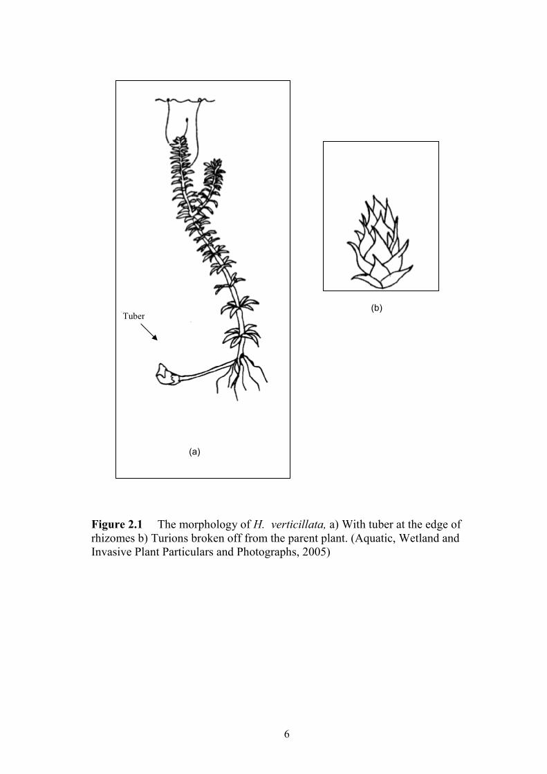
aboveground stems (stolons). It also forms hibernacula, turions in leaf axils and tubers
(subterranean turions) terminally on rhizomes. Turions are compact buds produced in the leaf
axils and they break off the parent plant when mature. They are 5 – 8 mm long, dark green and
spiny. Tubers are underground turions, which form at the end of rhizomes and can be found 30
cm deep in the sediment. They are 5 – 10 mm long and are white or yellowish (Langeland,
1996; Cook, 1996).
The leaves of Hydrilla verticillata are small, 2 – 4 mm wide, 6 – 20 mm long and occur
in whorls of 3 – 8 (Figure 2.1). They generally have 11- 39 sharp teeth per cm along the leaf
margin. They also often have spines or glands along the lower midrib of the leaf and are often

4
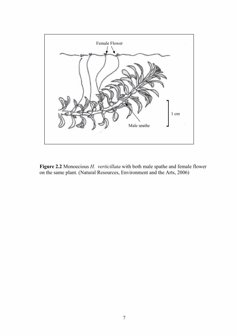
reddish in colour. Hydrilla verticillata can be monoecious (both male and female flowers on
the same plant) (Figure 2.2) or dioecious (male and female flowers on different plants) (Figure
2.3). Each male and female has its own unique growth characteristics. Male flowers have three
whitish red or brown sepals that are 3 mm long by 2 mm wide, and three whitish or reddish
linear petals about 2 mm long. They have three stamens, which forms in the leaf axils until they
break loose, at maturity and float to the surface where they free-float. Female flowers consist of
three translucent petals 10 – 50 mm long by 4 – 8 mm wide and three whitish sepals. They
grow attached to the leaf axils and float on the water surface (Langeland, 1996).
The list below shows the taxonomic classification of Hydrilla verticillata (L.f.) Royle
(Cook, 1996):
Kingdom : Plantae (Plants)
Subkingdom : Tracheobionta (Vascular plants)
Superdivision : Spermatophyta (Seed plants)
Division : Magnoliophyta (Flowering plants)
Class : Liliopsida (Monocotyledons)
Subclass : Alismatidae
Order : Hydrocharitales
Family : Hydrocharitaceae (Tape grass family)
Genus : Hydrilla
Species : Hydrilla verticillata (L. f.) Royle
Hydrilla verticillata closely resembles other members of its family such as Elodea
canadensis and Egeria densa. In 1995, Bowmer et al. distinguished H. verticillata from E.
canadensis by the number of leaves in the whorls, usually three in Elodea and four to six in
Hydrilla. While E. densa is distinguished by its larger leaves which is usually in whorls of four
or five. Hydrilla verticillata has been called Florida elodea, water thyme, lelumut (Leones et al.,
1991) and ‘same’ tree (Mansor, 1994).
5
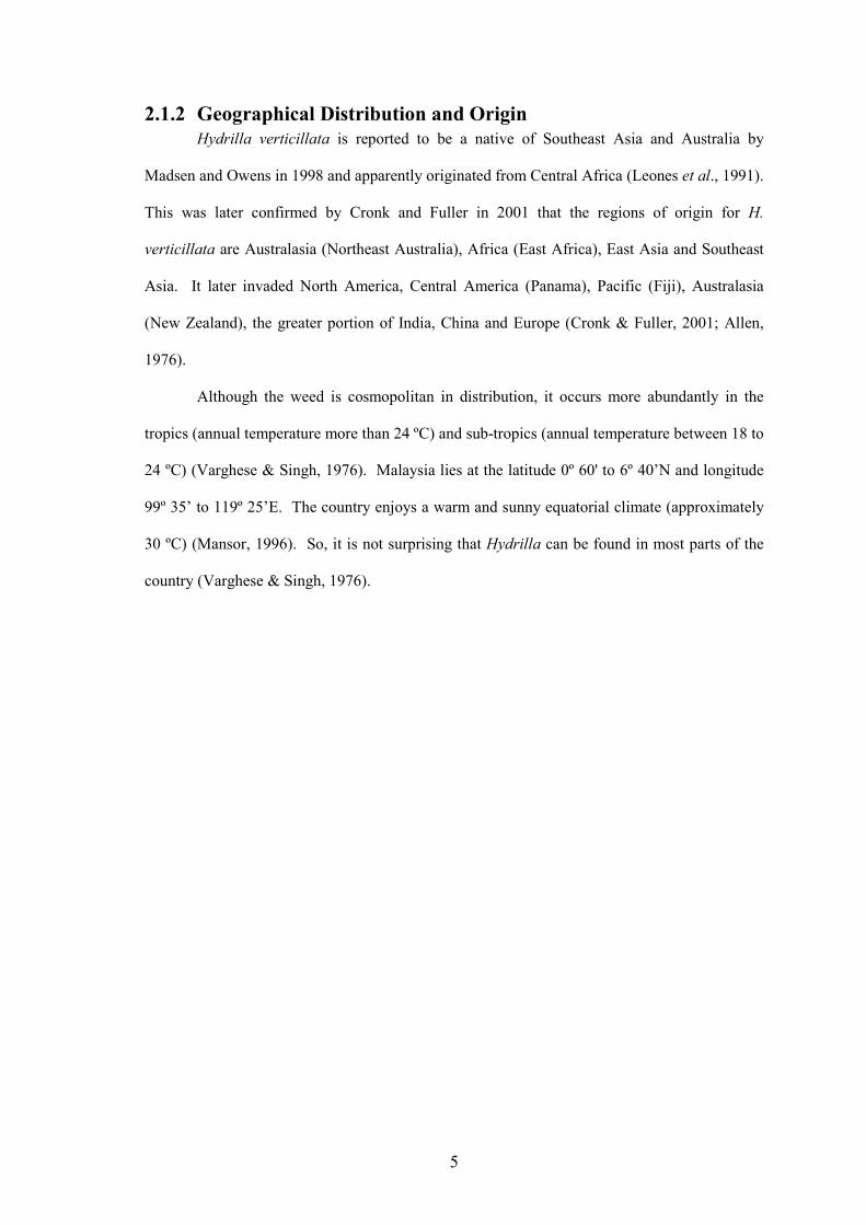
2.1.2 Geographical Distribution and Origin
Hydrilla verticillata is reported to be a native of Southeast Asia and Australia by
Madsen and Owens in 1998 and apparently originated from Central Africa (Leones et al., 1991).
This was later confirmed by Cronk and Fuller in 2001 that the regions of origin for H.
verticillata are Australasia (Northeast Australia), Africa (East Africa), East Asia and Southeast
Asia. It later invaded North America, Central America (Panama), Pacific (Fiji), Australasia
(New Zealand), the greater portion of India, China and Europe (Cronk & Fuller, 2001; Allen,
1976).
Although the weed is cosmopolitan in distribution, it occurs more abundantly in the
tropics (annual temperature more than 24 ºC) and sub-tropics (annual temperature between 18 to
24 ºC) (Varghese & Singh, 1976). Malaysia lies at the latitude 0º 60' to 6º 40’N and longitude
99º 35’ to 119º 25’E. The country enjoys a warm and sunny equatorial climate (approximately
30 ºC) (Mansor, 1996). So, it is not surprising that Hydrilla can be found in most parts of the
country (Varghese & Singh, 1976).
6
Figure 2.1 The morphology of H. verticillata, a) With tuber at the edge of rhizomes b) Turions broken off from the parent plant. (Aquatic, Wetland and Invasive Plant Particulars and Photographs, 2005)
(a)
Tuber (b)
7
Figure 2.2 Monoecious H. verticillata with both male spathe and female flower on the same plant. (Natural Resources, Environment and the Arts, 2006)
Female Flower
Male spathe
1 cm

8
Figure 2.3 Dioecious H. verticillata with female flowering shoot. (Aquatic and Wetland Plants of India, 1996)
1 cm
Female Flower

9
2.1.3 Biology and Physiology
Hydrilla verticillata has several physiological and morphological adaptations which
allow it to outcompete other aquatic plants. The ability of H. verticillata to grow under direct
sunlight at the water surface, as well as under canopy light, may be the factor that leads to its
success. A tolerance of low light conditions may enable H. verticillata to colonize deeper water
than other species (Hofstra et al., 1999), and this capability also enables H. verticillata to start
photosynthesis earlier in the morning. Comparison among three aquatic plant species (H.
verticillata, Vallisneria spiralis L. and Potamogeton pectinatus L.) proved that H. verticillata
showed minimum dark and photorespiration and maximum apparent photosynthesis with
vigorous growth (Jana and Choudhuri, 1979).
The availability of inorganic carbon for photosynthesis differs considerably in water
and air. This is because of slower diffusion rate of carbon dioxide in water than air (Casati et
al., 2000). So, aquatic autotrophs have to develop various ways to cope with limited carbon
dioxide and as well as high oxygen source (Magnin et al., 1997). Hydrilla verticillata is able to
switch from the C3 type mechanism to the C4 type carbon metabolism (fixing inorganic carbon
into malate and asparate) when the percentage of carbon dioxide is low (Rao et al., 2002).
According to Kahara and Vermaat (2003), H. verticillata can tolerate a wide range of
pH with the maximal pH tolerated being approximately pH 10.5. It can tolerate up to 7%
salinity of seawater and survive under limited nutrients such as carbon, nitrogen and phosphorus
(Langeland, 1996). Hydrilla verticillata can also store extra phosphorus for later use if
conditions are unfavorable. In short, the plant can survive in a wide range of environmental
regimes, whether in oligotropic (low nutrient) or eutropic (high nutrient) conditions.
Hydrilla verticillata has many effective means of propagation. There are four ways
(fragmentation, tubers, turions, seed production) of reproduction. Hydrilla verticillata
reproduces mainly by fragmentations. It can sprout new plants from stem fragments containing
as few as two nodes or whorls of leaves. Under unfavorable conditions, the plants propagate
itself asexually through stolons, tubers and turions (Leones et al., 1991). Hydrilla verticillata is
difficult to control because it produces axillary turions and tubers for regrowth after control of

10
the parent plants. Turions of monoecious H. verticillata can survive for 1 year under tank
conditions, but tubers can survive for a period of over four years (Sutton, 1996). The sexual
reproduction appears to be less important as compared to vegetative propagation. Hydrilla
verticillata is probably diploid (2n = 2x = 16) and sometimes endopolyploid, with triploid (2n =
3x = 24) and tetraploid (2n = 4x = 32) cells observed in the same populations (Langeland et al.,
1992).
2.1.4 Importance
As a problematic plant, H. verticillata always causes economic hardship wherever it
occurs. Examples in drainage and irrigation canals, the weed reduces the water flow and results
in higher water levels, greater loss of water by evaporation and inadequate supply of irrigation
water to rice fields (Mansor and Azinuddin, 1991). In addition, H. verticillata also interferes
with boating and navigation through the canals for both recreational and commercial purposes.
While the control of the weed will cost up to millions of ringgit, clearing task may also alter the
water quality and dissolved oxygen level. Although the changes of water chemistry is not too
destructive, but the effect on the habitat is quite pronounced (Mansor and Azinuddin, 1991).
Conversely, coupled with all the negative impact, H. verticillata also play an important
role in the fish populations. Ali (1988) suggested that, besides competing for nutrients and
blocking sunlight for photosynthesis, H. verticillata also able to inhibit zooplankton production.
However, these weeds also modify the predator-prey relationship among various zooplankton
groups as well as between zooplankton and fish (fish larvae, frys and adult fish) by providing
refuges for prey species to hide from predation. So the greater density of zooplankton observed
as weed biomass increased. The impact of this factor on fish population is quite significant and
extremely important to the success of fish population. This is because the year class strength of
fish population depends entirely on the initial survival of fish larvae and frys.

11
2.1.5 Management
There are a few control methods for H. verticillata, different type of water bodies have
to be treated differently and it depends on the end results required. Management or controlling
methods available are mechanical control, chemical control and biological control. In some
cases, physical control (manual removal) is favorable, but by using this method the weed is
never eradicated completely because it involves cutting only the top parts of the plants and not
the underground roots and buds.
There are harvester machines specially designed for mechanically removing H.
verticillata. Although this method is effective but the cost of the machine is high and can only
be used in large water bodies.
For chemical control, there are four commonly used active ingredients namely
fluridone, endothall, copper and diquat (Langeland, 1996). Different chemicals or combinations
of chemicals can be used to control Hydrilla verticillata at different levels. Fluridone
significantly inhibits the growth of H. verticillata, but the disadvantages using fluridone include
its high cost, slow-action, and non-selectivity toward other macrophyte species (Fox et al.,
1996; Hofstra and Clayton, 2001).
Endothall, a fast-acting contact herbicide, is used when immediate control of vegetation
is needed. Copper is used for its algicidal properties when heavy periphytic growth on the H.
verticillata may interfere with herbicide intake. Usually, to increase the efficiency of the
management system, dipotassium salt of endothall was often used in combination with diquat
(6,7-dihydrodipyrido (1,2-a : 2’, 1’-c) pyrazinediium dibromide, chelated copper or the
mono(N, Ndimethylalkalamine) salt of endothall. Pennington et al. (2001) proved that
herbicides applied in combination, specifically dipotassium salt of endothall/copper and
dipotassium salt of endothall/diquat, can provide excellent control of Hydrilla using lower
application rates. Apart from the four chemicals named, acetic acid has proven to be effective
in reducing survival of monoecious Hydrilla verticillata tubers (Spencer and Ksander, 1999).
Bensulfuron methyl also greatly inhibits the tuber formation of H. verticillata (Bowmer et al.,
1995).

12
Biological control is a technique that utilizes insects, microbial pathogens, or the
combination of them to manage the growth of H. verticillata. Hydrellia pakistanae is one of the
widely established biological control agent for H. verticillata (Wheeler and Center, 2001), and
its establishment is sufficient to impact the long-term growth of Hydrilla (Doyle et al., 2002).
Other potential biocontrol agents are H. verticillata leaf-mining fly, (Hydrellia balciunasi Bock)
and the H. verticillata stem boring weevil (Bagous hydrilla O’Brien) (Bowmer et al., 1995).
Paraponyx diminutalis (Lepidoptera: Pyralidae), an aquatic moth may also cause some damage
on H. verticillata but does not result in full control (Cronk and Fuller, 2001). Combination of
chemical fluridone with fungal pathogen (Mycoleptodiscus terrestris) greatly enhanced control,
reduced exposure requirement and increased the susceptibility of H. verticillata to fluridone
(Netherland and Shearer, 1996).
In 1998, Shearer once again tested the efficacy of Mycoleptodiscus terrestris against
dioecious H. verticillata and successfully found a biocarrier for this fungus. Another promising
biocontrol is triploid grass carp (Ctenopharyngodon idella Valenciennes). Killcore et al. (1998)
proved that grass carp effectively controlled Hydrilla but did not create any detectable negative
effects on the littoral fish assemblage. In search of the natural enemies of H. verticillata, two
insects were identified, Aphis sp. and &ymphula sp. Malaysia is believed to be the natural
habitat for this two insects (Varghese and Singh, 1976).
2.2 D�A MARKERS I� POPULATIO� GE�ETIC STUDY
2.2.1 Molecular Markers
In recent years, classical methods to evaluate genetic variation have been complemented
by molecular techniques. Allozyme markers were the first molecular markers that were used for
studying genetic variation within a number of species (Hoey et al., 1996; Sonnante et al., 1997).
Generally, allozyme markers which are co-dominant reveal polymorphism at the protein level
ie. heterozygotes can be distinguished from the homozygotes. But allozyme only detects
variations in protein coding loci, so only a portion of variation are estimated and this may not

13
reveal the true situation for the studied individual or population. In addition, the development
stage of a plant is one of the critical factors that are accounted for in this analysis.
Direct assessment at the DNA level is more sensitive and reliable. There are a whole
range of different DNA-based markers, that can be categorized into three aspects:
a. Non-PCR based approaches – Restriction fragment length polymorphism
(RFLP), Minisatellites, Variable Numbers of Tandem Repeats (VNTRs).
b. PCR based analysis – Microsatellites, RAPD, Inter-Simple-Sequence-Repeats
(ISSR), Inter-Retrotransposon Amplified Polymorphism (IRAP), AFLP.
c. DNA-sequence polymorphism – Single Nucleotide Polymorphism (SNP),
DNA-sequencing.
2.2.2 Random Amplified Polymorphic D�A
Random Amplified Polymorphic DNA (RAPD) developed by Williams et al. in 1990,
is one of the earliest DNA fingerprinting techniques that makes use of PCR. It is also known as
arbitrarily primed PCR. It gives a very quick and less expensive way to screen genetic diversity
in germplasms. RAPD became very popular because of its simplicity and wide applicability. It
is based on the amplification of random DNA segments using single primers of arbitrary
nucleotide sequence. Primers with ten nucleotides and a GC content of at least 50% are
generally used. Primers with lower GC content usually do not yield amplification products.
Because a G-C bond consists of three hydrogen brands and the A-T bond of only two, a primer-
DNA hybrid with less than 50% GC will probably not withstand the temperature at which
polymerization takes place (72oC). Therefore, the DNA-primer hybrid will have melted before
the polymerase has started polymerization. The amplification products are separated on an
agarose gel and detected by staining with ethidium bromide.

14
The enormous attraction of RAPD is due to several factors:
i. Only 25 nanogram of total genomic DNA are required as a starting material for
the analysis. This is particularly a good option if limited materials are
available, for example herbarium .
ii. Since the nucleotide order within the 10-mer primers is arbitrary, no
preliminary work, such as isolation of cloned DNA probes, preparation of
filters for hybridizations or prior knowledge of DNA sequences is needed. A
large number of potential markers can be generated using commercially
available primers (Mailer et al., 1994).
iii. RAPD assay are relatively quick, simple and less expensive. Only a
thermocycling machine and agarose gel apparatus are required in a laboratory.
It is a method of choice for analyses that requires bulking of genomic DNA or
less advanced laboratories (Paran et al., 1991; Upadhyay et al., 2004).
However, there are several difficulties and limitations with the approach:
i. The first concern is the nature of the data generated. RAPD are dominant
markers, the absence of a band represents the homozygous recessive, but the
presence of band cannot be differentiated between homozygous dominant or
heterozygotes. Therefore, in heterozygotes, the differences may appear only as
differences in band intensity, which is usually not reliable.
ii. The assumption that co-migrating bands represent homologous loci is
commonly made. A research by Rieseberg (1996) found out that 90% of the
bands that co-migrated on the same length in the agarose gel were truly
homologous when further examined with Southern hybridization or restriction
digest. To achieve the same degree of statistical power, on the order of 2 to 10
times more individuals need to be sampled per locus when dominant markers

15
are relied upon, as compared to co-dominant markers (Lynch and Milligan,
1994).
iii. Another general problem of RAPD is concerning the robustness of the data
generated. There are many factors that may influence its reproducibility, such
as size of primer, annealing temperature, template DNA quality and thermal
cycler used. Ramser et al. (1996) found that the main critical factor for
reproducibility turned out to be the quality of template DNA. According to
Skroch and Nienhuis (1995), reproducibility expressed as the percentage of
RAPD bands scored that are also scored in replicate data, was 76%. Although
statistical and physical differences may exist, they were not significant enough
to result in differences in genetic distance estimates greater than expected by
chance. After all, careful standardization and optimization in identical
amplification profiles proved to be reliable and highly reproducible (Heun and
Helentjaris, 1993; Lacerda et al., 2001; Shrestha et al., 2002).
The resolution of RAPD offers several potential applications in biological systems:
i. Assessment of genetic variation in populations and species. Similarity values
were generated and subjected in cluster analysis and analysis of molecular
variation (AMOVA). For example, Madeira et al. (2003) used RAPD analysis
to detect differences among geographically referenced samples of Salvinia
minima within and outside of Florida. The results showed that there is evidence
from PCO and AMOVA analysis that all the sampled populations can
somewhat group together according to chronologically infestation.
ii. To study relationships among species and subspecies. The determination of
taxonomic relatedness is only valid between taxa for which the diagnostic
RAPD fingerprint patterns have been established. Similarly, fragments
polymorphic at the species level will operationally identify members of a given

16
species if the fragment is constant among all members of that species (Hadrys
et al., 1992). Khan et al. (2000) reported that it is possible to differentiate very
closely related subspecies such as Gossypium herbaceum and Gossypium
herbaceum Africanum by using RAPD. Furthermore, most of the species can
be individually characterized with species-specific RAPD markers and these
results suggest that the RAPD technique produces reliable results with which to
construct the phylogenetic history of the genus Gossypium. Similarly, Ontivero
et al. (2000) showed that RAPD analysis provide useful data to recognize wild
strawberries and its related species in northwestern Argentina.
iii. To construct and understand genetic linkage maps, gene tagging, and
identification of cultivars. According to Ranade et al. (2001), gene tagging
using RAPD markers has at least three major advantages over other methods.
A universal set of primers can be used and screened in a short period, isolation
of cloned DNA probes or preparation of hybridization filters is not required and
only small quantity of genomic DNA is needed for each analysis. Gene tagging
and marker-assisted selection is an essential component of molecular breeding
and is based on saturation mapping of the genomes.
iv. Assignment of parentage. For example, Besse et al. (2004) used RAPD marker
to analyze the intergeneric hybrid of the genus Vanila Swartz.
Morphologically, Vanilla tahitensis is very similar to V. planifolia, but it
resembles V. pompona in its aromatic characteristics and the absece of fruit
dehiscence at maturity. Therefore, it was suggested that V. tahitensis could be
the result of a hybridization event between V. planifolia and V. pompona. This
hypothesis was confirmed to be wrong when RAPD results revealed that V.
tahitensis is probably not a species of direct hybrid origin (V. planifolia x V.
pompona) but rather a species

17
2.2.3 Amplified Fragment Length Polymorphism
In 1995, Keygene Inc. developed a novel DNA fingerprinting technique termed
Amplified Fragment Length Polymorphism (AFLP) (Vos et al., 1995). This procedure is
essentially a combination of RFLP and RAPD. It is based on the detection of genomic
restriction fragments and followed by PCR amplification. The technique involves three steps:
(1) restriction of the genomic DNA and ligation of oligonucleotide adaptors (2) selective
amplification of a subset of all the fragments in the total digest and (3) gel-based analysis of the
amplified fragments.
The first step requires genomic DNA to be digested by two restriction endonucleases,
one a rare cutter and the other a frequent cutter. A frequent cutter will generate small sizes of
DNA fragments, which are excellent for amplification and the optimal size range for separation
on denaturing gel. While a rare cutter is to reduce the number of DNA fragments to be
amplified. Too many fragments for resolution by gel electrophoresis will create
indistinguishable bands. Double stranded adaptors are then added to the ends of the digested
DNA fragments to provide known sequences for PCR amplification.
Although the numbers of fragments have been reduced, there are thousands of adapted
fragments, depending on the genome size. The number of fragments obtained increased as the
genome size increased. A stricter selection is required to achieve the ideal number of fragments
within the range that can be resolved on a single gel. Thus, primers are designed to incorporate
the known adaptor sequence plus one to three arbitrarily chosen base pairs. Fewer fragments
will be amplified with more additional nucleotides. Normally PCR will be carried out twice.
The first time, pre-selective; only one selective nucleotide is used. The second time, selective
PCR, the same selective nucleotide plus one or two additional ones are used.
There is a variety of techniques that can be used to visualize the amplified products.
Ranging from the simplest way i.e. agarose gel electrophoresis to automated genotyping.
Polyacrylamide gel electrophoresis (manual or automated) is sufficient to separate the fragments
even to a single base pair difference. An automation of AFLP genotyping that allows the use of

18
an internal lane size standard will ensure superior sizing accuracy with no lane-to-lane or gel-to-
gel variation.
Two different types of polymorphism can be detected with AFLP: (1) point mutation in
the restriction sites, or in the selective nucleotides of the primers which results in a signal in one
case and absence of a band in the other, and (2) small insertion or deletions within the
restriction fragment which results in different sized bands.
AFLP markers offer the following advantages:
i. It markers can be applied to any organism and no prior knowledge about the
genomic makeup of the organism needed.
ii. It can be generated at great speed.
iii. AFLP analysis requires minimal amounts of DNA and is insensitive to the
template DNA concentration. Therefore, DNA quantities that vary between
individual samples will not affect the end results of AFLP analysis (Vos et al.,
1995).
iv. The AFLP method is less problematic than RAPD technique, AFLP
amplification is performed under conditions of high stringency, thus eliminating
nonspecific binding and artefactual variation (Parsons and Shaw, 2001).
v. This technique is highly reproducible and provides nearly unlimited number of
informative markers that spread over the entire nuclear genome. As it is, AFLP
markers will be located in variable regions and even low genetic variability can
be detected within any given group of organism (Hodkinson et al., 2000;
Hedren et al., 2001; Després et al., 2003).
The high reliability of AFLP and unparalleled sensitivity to minor genetic differences
make them valuable in diversity studies. AFLP markers have been proved useful for: (1)
systematics and biodiversity surveys, (2) population and conservation genetics, (3) kinship and
parentage analysis and (4) QTL mapping (Quantitative Trait Loci).

19
2.2.4 The reasons for using RAPD and AFLP
Genetic diversity in H. verticillata accession from most part of the world has been
studied using isoenzyme markers (Madeira et al., 1997; Madeira et al., 1999; Hofstra et al.,
2000). However, isoenzymes are less sensitive to genomic changes and it is limited by the
functional enzymes in the coding region which is a relatively small number of loci (Angel,
2002).
By the year 1997, Madeira et al. have successfully studied the relationships among 44
accessions of H. verticillata from places around the world using RAPD. From their
experiments, it was proven that RAPD is a useful tool for examining the inter-relationships of
Hydrilla accessions. In the year 2000, isozyme together with RAPD was used to assess the
genetic structure within and between four populations of Hydrilla in New Zealand. The RAPD
results were congruent with the isozyme results. It shows that there was no variation within and
between samples from four different populations in New Zealand and this is because the genetic
diversity among populations is very low (Hofstra et al., 2000).
In the present study, RAPD technique was employed, as it has been successfully
utilized in H. verticillata. In addition AFLP technique was also used since it has been
suggested to perform well for plants that showed low genetic variability using RAPD. AFLP is
used to complement the RAPD technique. Both RAPD and AFLP have advantages and
disadvantages for assessing genetic diversity, and many studies have demonstrated the high
potential of the two markers for population studies (Madeira et al., 1997; Kristen et al., 1998;
Madeira et al., 1999; Hofstra, 2000; Angel, 2002; Madeira et al., 2003; Martin et al., 2003; Li
and Jin, 2006). It is hoped that the use of these two markers will provide a better resolution of
genetic diversity of H. verticillata in Malaysia.
20
CHAPTER THREE
MATERIALS & METHODS
3.1 PLA�T SAMPLES
3.1.1 Sample Collection
Hydrilla verticillata was collected from all types of water bodies in Malaysia.
Individual rooted shoots, totaling three to ten, were collected randomly and removed carefully
from the substrate. After collection, samples were kept in plastic bags with its native water
before transferring to the laboratory. The epiphytes were washed with water and blotted on
paper towel. Samples were then placed into zipper bags containing silica gel desiccant. The
desiccant was changed regularly to make sure the samples were totally dried. They were then
kept in the freezer at temperature of –20 ˚C until removed for DNA extraction.
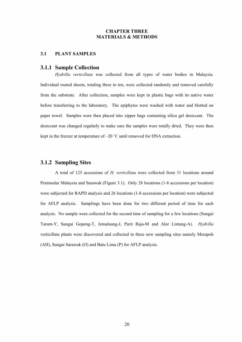
3.1.2 Sampling Sites
A total of 125 accessions of H. verticillata were collected from 31 locations around
Peninsular Malaysia and Sarawak (Figure 3.1). Only 28 locations (1-8 accessions per location)
were subjected for RAPD analysis and 26 locations (1-8 accessions per location) were subjected
for AFLP analysis. Samplings have been done for two different period of time for each
analysis. No sample were collected for the second time of sampling for a few locations (Sungai
Tarum-Y, Sungai Gopeng-T, Jemaluang-J, Parit Raja-M and Alor Lintang-A). Hydrilla
verticillata plants were discovered and collected in three new sampling sites namely Merapoh
(AH), Sungai Sarawak (O) and Batu Lima (P) for AFLP analysis.

21
G F
E
D
AD AE AF AG V Z
AA
T
X
B
A
AH
S
R
N
I M
J
K
N
Scale 1 : 3, 125, 000
O km 50 100 150 7º N
6º N
5º N
4º N
3º N
2º N
1º N 103º E 104º E 102º E 101º E 100º E
SOUTH CHINA SEA
STRAIT OF MALACCA
U
L
Figure 3.1 The 28 sampling sites of Hydrilla verticillata around Peninsular Malaysia. Three sampling sites from Sarawak (Bintawa-Q, Sungai Sarawak-O and Batu Lima-P) were not shown in the map. Code and number assigned in the map is described in Table 3.1 and Table 3.3.
W AB

22
3.1.3 D�A Extraction
DNA was extracted using the CTAB (cetyltrimethylammonium bromide) standard
extraction procedure as described by Doyle and Doyle (1987) with minor modifications. 0.2 –
0.4g of silica gel-dried leaf sample was quickly frozen in liquid nitrogen and ground to fine
powder using a mortar and pestle. 4 ml of preheated (55˚C) 2X CTAB extraction buffer (1.4M
NaCl, 20mM EDTA at pH 8.0, 2% CTAB, 1% PVP, 0.1M Tris at pH 8.0 and 1 % β-
mercaptoethonol) was added to the fine powder and transferred to a 10 ml clean tube. The
suspension was incubated at 55˚C water bath for 30 minutes with occasional shaking to produce
an homogenous solution.
The tube was cooled 5 minutes at room temperature. The mixture was emulsified by
adding 2 ml of chloroform: isoamyl alcohol (24:1, v/v). Tube was spun at 4000 rpm for 10
minutes. The top aqueous layer was transferred to a clean tube then 2 ml of chloroform:
isoamyl alcohol (24:1, v/v) and one ten volume of 10% CTAB was added into the supernatant.
The tube was shaken vigorously before centrifuged at 4000 rpm for 10 minutes. Only 600 µl of
the upper layer were transferred to each of four new 1.5 ml microcentrifuge tubes which
contained two third volumes of cold isopropanol. The mixture was mixed by several inversions
of the tubes.
Precipitated DNA can be observed at the bottom of the tubes as a transparent pellet after
centrifugation at 10 000 rpm for 30 minutes. 600 µl of 76% ethanol/0.2M NaAc was added to
the DNA pellet and it was left to stand at room temperature for 50 minutes. The supernatant
was discarded and 300 µl of 76% ethanol/10 mM NH4Ac was added to wash the DNA pellet.
Ethanol was poured out and the DNA pellet was left to air dry by inverting the tubes on a paper
towel. DNA was dissolved in 50 µl sterile distilled water at 4˚C overnight.

23
3.1.4 D�A Repurification
Extracted DNA was purified with ammonium acetate. 50 µl aliquot of the same DNA
sample from four tubes were combined into a single 1.5 ml microcentrifuge tube resulting in a
total volume of 200 µl. 100 µl of cold 7.5M NH4Ac was later added to the tube. The tube was
incubated at -4˚C for 15-20 minutes and centrifuged at 10 000 rpm for 15 minutes. The
supernatant was removed using a sterile pipette tip and transferred into a new 1.5 ml
microcentrifuge tube. DNA was precipitated using 2 volume of cold 95% ethanol, kept in -4˚C
for 30 minutes and centrifuged again at 10 000 rpm for 15 minutes. The resulting pellet was
washed with 350 µl cold 70% ethanol and centrifuged at 10 000 rpm for 15 minutes. The
pelleted DNA was air dried and resuspened in 100 µl sterile distilled water at 4˚C overnight.
3.1.5 Quantification of D�A Samples
DNA yield and quality was assessed by gel electrophoresis and measured
spectrophotometrically (Eppendorf Biophotometer 6131).
a) Evaluating DNA Quality by Gel Electrophoresis
The quality of the DNA was evaluated by electrophoresis in 0.8% agarose gel. 1 µl of
6X loading buffer (Fermentas) was applied to each 5 µl of DNA and loaded into each well. The
electrophoresis was allowed to run at 80V for 1 hour in 0.5X TBE buffer and stained with
ethidium bromide (1 µg/ml). The gel was visualized under a UV light transilluminator. Only
samples yielding predominantly high quality DNA were included in the study.
b) Determination of DNA Concentration
The optical density for the extracted DNA samples was determined with
spectrophotometer. The absorbance of the samples was read at wavelength 260 nm, 280 nm and
320 nm with Eppendorf Biophotometer 6131. Good quality DNA has a ratio value of
OD260/OD280 between 1.8 to 2.0. A ratio of less than 1.8 is indicative of contamination by
protein and a value of more than 2.0 shows RNA contamination.

24
3.2 RAPD A�ALYSIS PROTOCOL
3.2.1 Materials
A total of 119 accessions (1-8 accessions per populations) from 28 populations were
subjected to RAPD analysis. Code and number assigned for each accession of every location
are given in Table 3.1 and is referred in text and figure for comparisons.
3.2.2 Primer Screening
One hundred and twenty of random primers from four primer sets namely OPA, OPE,
OPF, and OPH (MWG Biotech AG) (Appendix A) while two primer sets OPB and OPG
(Operon Technologies) (Appendix B) were being screened. Two samples from the same
location and one sample from a distant location were chosen to carry out the initial screening of
primers. Primers were chosen based on the clarity and reproducibility of banding patterns in
preliminary screening and were used for further analysis.

25
Table 3.1 Plant materials for RAPD analysis. Populations Sample size Code and number assigned Northern Peninsular D - Sungai Petani, Kedah 2 D1, D2 E - Simpang Tiga, Kedah 1 E1 F - Sungai Kok Mak (Padang Besar), Perlis
6 F1, F2, F3, F4, F5, F6
G - Sungai Korok (Padang Besar), Perlis
5 G1, G3, G4, G7, G9
Y - Sungai Tarum (Langkawi), Kedah
5 Y1, Y2, Y3, Y4, Y5
AD - Sungai Burung (Balik Pulau), Pulau Pinang
6 AD1, AD2, AD3, AD4, AD5, AD6
AE - Sungai Bayan Lepas (Bayan Lepas), Pulau Pinang
6 AE1, AE2, AE3, AE4, AE5, AE6
AF - Sungai Kampung Masjid (Bayan Lepas), Pulau Pinang
6 AF1, AF2, AF3, AF4, AF5, AF6
AG - Sungai Buaya (Balik Pulau), Pulau Pinang
4 AG1, AG3, AG4, AG6
West Coast V - Nibong Tebal, Pulau Pinang 4 V1, V2, V3, V4 AA - Bukit Panchor, Perak 3 AA1, AA2, AA4 Z -Selama, Perak 5 Z2, Z3, Z4, Z5, Z6 U - Simpang Lima, Perak 1 U1 W - Bagan Serai, Perak 5 W2, W3, W4, W5, W6 AB - Semanggol, Perak 7 AB1, AB2, AB3, AB4, AB5, AB6, AB7 T - Sungai Gopeng, Perak 3 T1, T2, T3 X – Temoh, Perak 7 X1, X2, X3, X4, X5, X6, X7 S - Tanjung Karang, Selangor 8 S1, S2, S3, S4, S5, S6, S7, S8 R - Pantai Belimbing, Melaka 4 R1, R2, R4, R5 Southern Peninsular I - Parit Besar, Johor 3 I1, I2, I3 J – Jemaluang, Johor 2 J1, J2 K - Sungai Bang (Kota Tinggi), Johor
3 K1, K2, K3
L - Ayer Hitam, Johor 5 L1, L2, L3, L5, L6 M - Parit Raja (Batu Pahat), Johor
5 M1, M2, M3, M4, M5
N - Sungai Sialang (Tangkak), Johor
5 N1, N3, N5, N6, N8
East Coast A - Alor Lintang, Terengganu 4 A1, A2, A3, A6 B - Sungai Terah (Gua Musang), Kelantan
3 B2, B3, B4
Sarawak Q - Bintawa (Kuching), Sarawak
1 Q1