by

Steven F. Bartlett

Daniel Gillins

April 9th, 2104

EERI

Outline

Modification to Lateral Spread Model

Interpreting and Use CPT Data in

Revised Model

Monte Carlo Method

Mapping Inputs

Map Examples

Youd et al. (2002) Empirical Model

Seismic Factors

M, R

Topographic Factors

W, S

Geotechnical Factors

T15 , F15 , D5015

1 2 3 4 5 6 15

7 15 8 15

*

(100 ) ( 50 0.1 mm)

o off

H

b b b M b LogR b R b LogW b LogS b LogTLogD

b Log F b Log D

Free-face ratio: W (%) = H / L * 100

New Empirical Model

1 2 3 4 5

6 15 1 1 2 2 3 3 4 4 5 5

*o off

H

b b b M b LogR b R b LogW b LogSLogD

b LogT a x a x a x a x a x

xi = the portion (decimal fraction) of T15 in a borehole that

has a soil index corresponding to the table below

(SI) equal to i Soil Index

(SI)

Typical Soil Description in Case

History Database

General

USCS

Symbol

1 Silty gravel, fine gravel GM

2 Coarse sand, sand and gravel GM-SP

3 Medium to fine sand, sand with some silt SP-SM

4 Fine to very fine sand, silty sand SM

5 Low plasticity silt, sandy silt ML

6 Clay (not liquefiable) CL-CH

Comparing the Models

Model R2 (%) MSE σlogDH P-Value

Full: Youd et al. (2002) 83.6 0.0388 0.1970 0.000

Reduced: no F15 or D5015 66.6 0.0785 0.2802 0.000

New: with soil type terms 80.0 0.0476 0.2182 0.000

Youd et al. (2002) Gillins and Bartlett (2013)

Cone Penetrometer Test (CPT)

Estimating N1,60 from CPT Data

Estimating xi Variables with CPT

2 2 0.5[(3.47 ) ( 1.22) ]c tn rI LogQ LogF

Robertson (1990) Soil

Behavior Type Chart

Boundaries of each zone

estimated by circles with

radius = Ic

Histograms of Ic for each SI

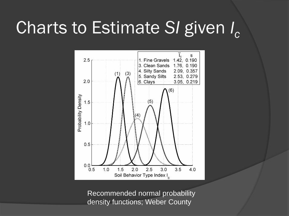
Charts to Estimate SI given Ic

Recommended normal probability

density functions; Weber County

Example 1

i P

1. Fine Gravels 0.63

3. Clean Sands 0.27

4. Silty Sands 0.09

5. Sandy Silts 0.00

6. Clays 0.00

Find probability that:

SI = 1 (i.e., fine gravel)

given Ic = 1.5

P (SI = i | Ic = 1.5 ):

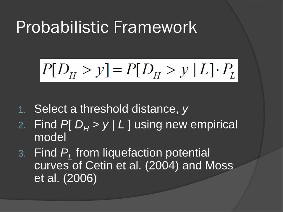
Probabilistic Framework

1. Select a threshold distance, y

2. Find P[ DH > y | L ] using new empirical model

3. Find PL from liquefaction potential curves of Cetin et al. (2004) and Moss et al. (2006)

Example 2

SPT-based Liquefaction Potential

Curves (Cetin et al., 2004)

Find P [ DH > 1 m] given:

CSR = 0.1; N1,60,cs = 10

M = 7.5; R = 20 km

S = 0.5 %

T15,cs = 1 m; σ’v = 1 atm

0.00

0.25

0.50

0.75

1.00

0 10 20 30

PL

N1,60,cs

PL = 0.76

Example 2 (cont.)

P [ DH > y ] = (0.33)*(0.76) = 0.25

= Φ ( - z )

= 0.33

“Simple calculations based

on a range of variables are

better than elaborate ones

based on limited input.”

-Ralph B. Peck

Monte Carlo Technique

Used when:

Unable to compute results deterministically

Systems have many degrees of freedom

Modeling phenomena with significant uncertainty

1) Define a domain of inputs

2) Generate inputs randomly from a probability distribution over the domain;

3) Perform a deterministic computation on the inputs;

4) Aggregate the results to define the median values and their uncertainty

The Normal Distribution

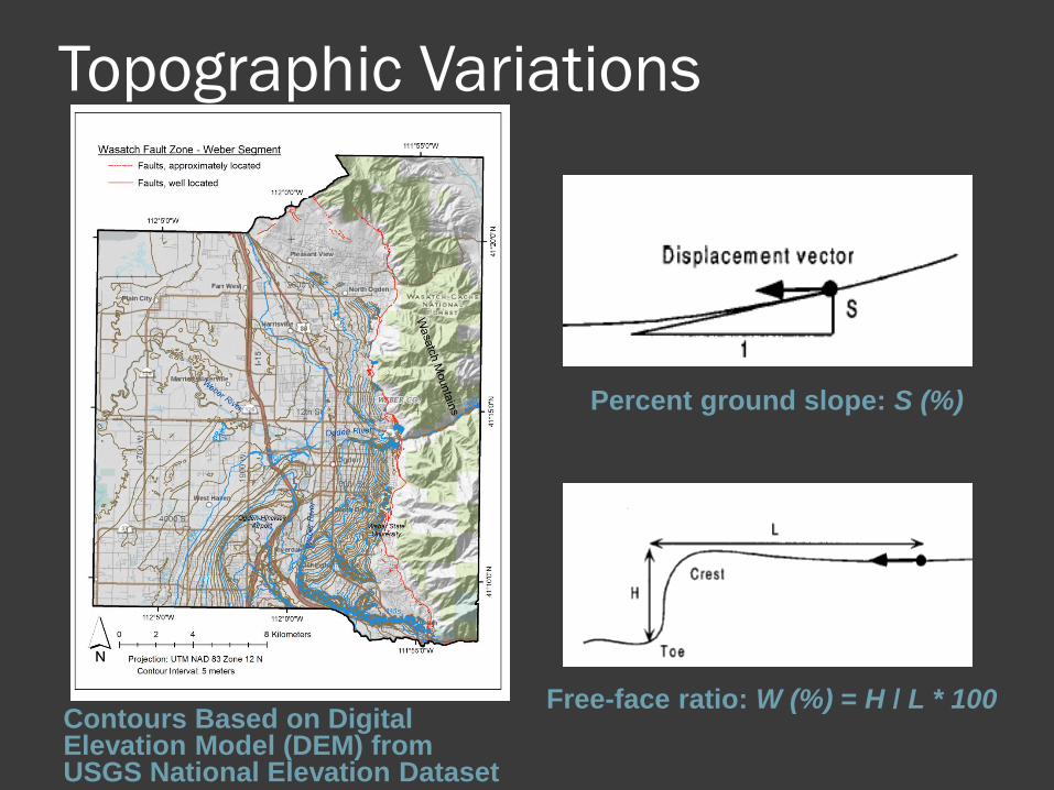
Topographic Variations

Contours Based on Digital Elevation Model (DEM) from USGS National Elevation Dataset

Free-face ratio: W (%) = H / L * 100

Percent ground slope: S (%)

Seismic Inputs

Mean seismic variables from interactive deaggragation of the seismic hazard

Seismic hazard based on 2008 source and attenuation models of the National Seismic Hazard Mapping Project (Peterson et al., 2008)

Liquefaction Triggering Maps

Median probabilities of PL, 500-

year seismic event

Median probabilities of PL, 2,500-

year seismic event

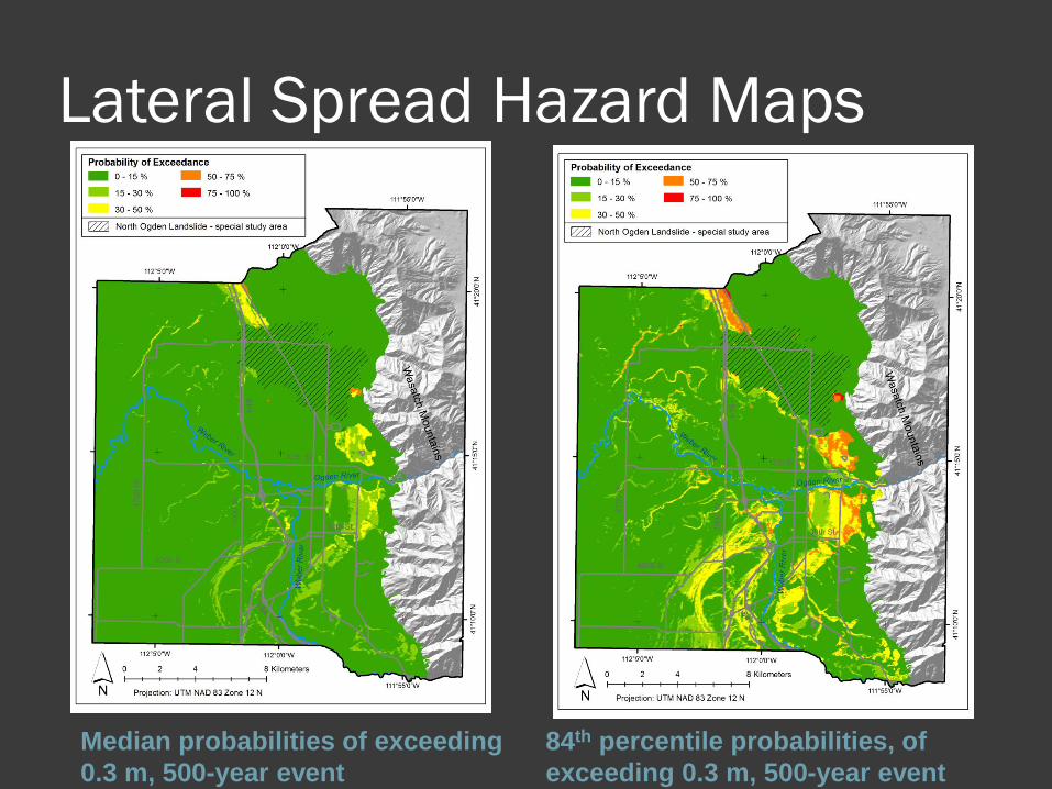
Lateral Spread Hazard Maps

Median probabilities of exceeding

0.3 m, 500-year event

84th percentile probabilities, of

exceeding 0.3 m, 500-year event

Lateral Spread Hazard Maps

Median probabilities of exceeding

0.3 m, 2,500-year event

84th percentile probabilities, of

exceeding 0.3 m, 2,500-year event

For more information:

http://www.civil.utah.edu/~bartlett/ULAG/