Business Process SimulationLecture notes 2II75

W.M.P. van der Aalst and M. VoorhoeveDept. of Mathematics and Computer Science,

Technical University Eindhoven,Postbox 513, 5600 MB, Eindhoven.

PrefaceThese lecture notes are based on a document (Handboek simulatie) in Dutch fromthe first author. It has been translated, revised and adapted as course material bythe second author.

The examples and exercises are based on the Arena package [5].A downgraded student version of Arena can be downloaded from the directory//campusmp/software/rockwell. This version suffices to view, modify, create andsimulate the models of this course. The Arena example models in the exercises canbe found at www.win.tue.nl/˜mvoorhoe/sim.

The simulation course is intended for systems engineering students with modelingexperience and a basic knowledge of probability theory and statistics. Students areexpected to be have some experience in Petri net modeling, as e.g. taught in thecourse 2V060 (systems modeling 1). A recapitulation of the principles can be foundin Appendix A.

1

Contents

1 Introduction 4

2 Conducting a simulation project 6

3 Problem definition and analysis 11

4 Modeling 124.1 Conceptual Modeling . . . . . . . . . . . . . . . . . . . . . . . . . . . 12

4.1.1 Ferry example . . . . . . . . . . . . . . . . . . . . . . . . . . 134.1.2 Photo example . . . . . . . . . . . . . . . . . . . . . . . . . . 14

4.2 Implementing the conceptual model . . . . . . . . . . . . . . . . . . 174.2.1 Ferry example . . . . . . . . . . . . . . . . . . . . . . . . . . 184.2.2 Photo example . . . . . . . . . . . . . . . . . . . . . . . . . . 19

5 Parameterizing the models 21

6 Processing the results 246.1 Observed quantities . . . . . . . . . . . . . . . . . . . . . . . . . . . 246.2 Subruns and preliminary run . . . . . . . . . . . . . . . . . . . . . . 25

6.2.1 Necessity . . . . . . . . . . . . . . . . . . . . . . . . . . . . . 256.2.2 Subruns and initial phenomena . . . . . . . . . . . . . . . . . 26

6.3 Analysis of subruns . . . . . . . . . . . . . . . . . . . . . . . . . . . . 276.3.1 The situation with over 30 subruns . . . . . . . . . . . . . . . 286.3.2 The situation with less than 30 subruns . . . . . . . . . . . . 30

6.4 Variance reduction . . . . . . . . . . . . . . . . . . . . . . . . . . . . 316.5 Sensitivity analysis . . . . . . . . . . . . . . . . . . . . . . . . . . . . 33

7 Pitfalls 33

8 Recommended further reading 37

A Modeling, concurrency and scheduling with Petri nets 39

B Basic probability theory and statistics 42B.1 Random and pseudo-random numbers . . . . . . . . . . . . . . . . . 42B.2 Probability distributions . . . . . . . . . . . . . . . . . . . . . . . . . 43

C Discrete random distributions 44C.1 Bernoulli distribution . . . . . . . . . . . . . . . . . . . . . . . . . . 45C.2 Discrete homogeneous distribution . . . . . . . . . . . . . . . . . . . 45C.3 Binomial distribution . . . . . . . . . . . . . . . . . . . . . . . . . . . 45C.4 Geometrical distribution . . . . . . . . . . . . . . . . . . . . . . . . . 46

2

C.5 Poisson distribution . . . . . . . . . . . . . . . . . . . . . . . . . . . 46

D Continuous random distributions 46D.1 Uniform distribution . . . . . . . . . . . . . . . . . . . . . . . . . . . 47D.2 Triangular distribution . . . . . . . . . . . . . . . . . . . . . . . . . . 47D.3 Negative exponential distribution . . . . . . . . . . . . . . . . . . . . 47D.4 Normal distribution . . . . . . . . . . . . . . . . . . . . . . . . . . . 49D.5 Gamma distribution . . . . . . . . . . . . . . . . . . . . . . . . . . . 50D.6 Erlang distribution . . . . . . . . . . . . . . . . . . . . . . . . . . . . 50D.7 χ2 distribution . . . . . . . . . . . . . . . . . . . . . . . . . . . . . . 52D.8 Beta distribution . . . . . . . . . . . . . . . . . . . . . . . . . . . . . 54

E Random variables 56

F Queuing models 58

3

1 Introduction

Suppose you run a discotheque and have problems in deploying staff on Saturdaynights. At certain times there is too much staff capacity, however customers com-plain about long waiting times for getting their coats hung up and ordering drinks.Because you feel you are employing too much staff and yet face the threat of losingcustomers due to excessive waiting times, you decide to make a thorough investiga-tion. Examples of questions you want answered are:

• What are the average waiting times of customers at the bars and the cloak-room?

• What is the occupation rate of the bar staff?

• Will waiting times be reduced substantially if extra staff is deployed?

• Would it serve a purpose to deploy staff flexibly? (e.g. no longer assigningstaff members to one bar only)

• What is the effect of introducing refreshment coupons on average waitingtimes?

• What are the effects of introducing a ‘happy hour’ to spread the arrivals ofguests?

To answer these and similar questions, simulation can be used. A model is built thatSimulationSimulationmodel

reflects reality and is used to simulate that reality in a computer. In the same waythat an architect uses construction drawings to understand a building, a systemsanalyst may use simulation models to assess a business process.

When is simulation appropriate? Some reasons are:Reasons forsimulation

• Gaining insight in an existing or proposed future situation. By charting andsimulating a business process, it becomes apparent which parts are critical.These parts can then be examined more closely.

• A real experiment is too expensive. Simulation is a cost-effective way to analyzeseveral alternatives. Trial and error is not an option when it comes to hiringextra staff or introducing a refreshment coupon system. You want to make surein advance whether a certain measure will have the desired effect. Especiallywhen starting up a new business process, simulation can save a lot of money.

• A real experiment is too dangerous. Some experiments cannot be carried outin reality. Before a railway company installs a new traffic guidance system, itmust assess the safety consequences. It must be noted, however, that simula-tion alone cannot address safety issues. The safety itself must be addressed byformal analysis techniques, whereas simulation can assist in assessing e.g. theperformance. The same holds for other processes where safety is critical (e.g.aviation or nuclear reactors).

4

Sometimes, rather than using simulation, a mathematical model, also called ananalytical model is sufficient. In Operations Research (OR) many models havebeen developed which can be analyzed without simulation, such as queuing models,optimization models or stochastic models. It is advisable to address a simplifiedversion of the problem at hand by an analytical model and compute its characteristicsbefore conducting a simulation study on the full problem. The analysis gives extrainsight from which the simulation study can profit. Also, the analysis results providea reference for the expected simulation results, so that simulation errors can beavoided as much as possible. If the outcome of the simulation experiments deviatesfrom the computed characteristics, one should find reasons for the difference.In this course, we shall discuss some simple analysis methods that can often be usedto support simulation. More advanced analysis methods, requiring considerableknowledge and effort, can and should be used in certain cases. Strong points ofsimulation versus analysis:Advantages

ofsimulation • Simulation is flexible. Any situation, no matter how complex, can be investi-

gated through simulation.

• Simulation can be used to answer a variety of questions. It is possible to assesse.g. waiting times, occupation rates and fault percentages from one and thesame model.

• Simulation is easy to understand. In essence, it is nothing but replaying amodeled situation. In contrast to many analytical models, little specialistknowledge is necessary to understand the model.

Simulation also has some disadvantages.Disadvantagesofsimulation

• A simulation study can be very time consuming. Sometimes, very long simu-lation runs are necessary to achieve reliable results.

• One has to be very careful in interpreting simulation results. Determining thereliability of results can be very treacherous indeed.

• Simulation does not offer proofs. Whatever occurs in a correct simulationmodel may occur in reality, but the reverse does not hold. Things may happenin reality that have not been witnessed during simulation.

For the construction of a simulation model we use a tool , which ensures that theSimulationtools computer can simulate the situation charted by the model. Tools can be languages

or graphical packages.

Simulation languages A simulation language is a programming language withspecial provisions for simulation, such as Simula.

Simulation packages A simulation package is a tool with building blocks allowingthe assembly of a simulation model. There are special-purpose packages forcertain application areas, such as Taylor II, (production) and more generalpackages like Arena.

5

The advantage of a simulation language is extreme flexibility, but at the cost ofclarity and a considerable programming effort. The use of a simulation package cor-responds to graphical modeling with building blocks that need to be parameterized.The more general (and flexible) the package, the more parameters are needed.Often it is desirable to combine various techniques, such as a Taylor manufactur-ing model with a language-based scheduling algorithm. By means of conceptualmodeling, insight is obtained in the various aspects of the system that needs to bemodeled. From such a conceptual model, a simulation tool can be selected and usedto construct the executable simulation model.————————–A civil servant creates documents for citizens, who are queueing for his help. On average,Photo

example a new citizen needing help arrives every 5 minutes. A photo must be attached to the doc-ument, which is judged by the servant. The judgement takes 1 minute on average. In 40%of the cases, the photo is judged inadequate, upon which the citizen is deferred to a nearbyphotographer to make a new one. This advice takes on average 1.5 minutes, after whichthe next citizen is helped. It takes on average 20 minutes to obtain a new photo; whenthe citizen returns with it, he gets priority for his document and the photo is immediatelyjudged correct. Making the document takes on average 3.5 minutes.

Exercise The Arena model gemeente.doe (at www.win.tue.nl/˜mvoorhoe/sim) contains amodel of the photo example sketched above.You are asked to conduct a simulation to assess the occupation rate of the civilservant. Open the Arena file and press the I (run) button and observe thebehavior. When you have seen enough, press the II (fast-forward) button.When the simulation is completed, you are looking at the state after 1000 hoursof simulation. To find the requested occupation rate, open the Reports tab at theleft and then the Resources report. Under the instantaneous utilization Inst Utilcolumn, the answer (0.97) can be found. Why is this number incorrect? Is ituseful at all to simulate the sketched situation?

2 Conducting a simulation project

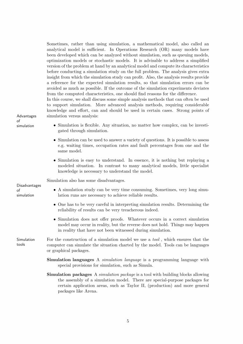
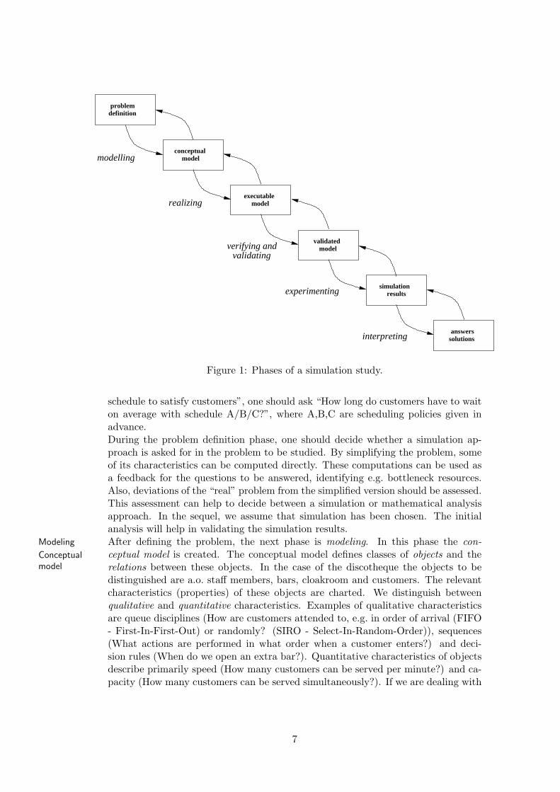
Simulation is often used to support strategic decisions. This requires a properproject-oriented approach, consisting of problem analysis, model construction, sim-ulating and interpreting the results as illustrated in Fig 1). User-friendly tools mayallow rapid prototyping, but it is dangerous to base important decisions on proto-types.An often used “waterfall” approach that illustrates the phasing of a simulationPhasing

project is depicted in Figure 1. Note that a phase can start before completingits predecessors and that it can be influenced by its successors. We give a shortdescription of every phase.

The simulation project starts with a problem definition , describing the goals andProblemdefinition fixing the scope of the simulation study. The scope tells what will and what will

not be a part of the simulation model. The problem definition should also statethe questions to be answered. These questions should be quantifiable and focuson selection rather than optimization. Instead of asking “what is the best bar

6

answerssolutions

validated

modelling

realizing

verifying andvalidating

experimenting

interpreting

simulation

model

modelexecutable

conceptual

results

problemdefinition

model

Figure 1: Phases of a simulation study.

schedule to satisfy customers”, one should ask “How long do customers have to waiton average with schedule A/B/C?”, where A,B,C are scheduling policies given inadvance.During the problem definition phase, one should decide whether a simulation ap-proach is asked for in the problem to be studied. By simplifying the problem, someof its characteristics can be computed directly. These computations can be used asa feedback for the questions to be answered, identifying e.g. bottleneck resources.Also, deviations of the “real” problem from the simplified version should be assessed.This assessment can help to decide between a simulation or mathematical analysisapproach. In the sequel, we assume that simulation has been chosen. The initialanalysis will help in validating the simulation results.After defining the problem, the next phase is modeling. In this phase the con-Modeling

ceptual model is created. The conceptual model defines classes of objects and theConceptualmodel relations between these objects. In the case of the discotheque the objects to be

distinguished are a.o. staff members, bars, cloakroom and customers. The relevantcharacteristics (properties) of these objects are charted. We distinguish betweenqualitative and quantitative characteristics. Examples of qualitative characteristicsare queue disciplines (How are customers attended to, e.g. in order of arrival (FIFO- First-In-First-Out) or randomly? (SIRO - Select-In-Random-Order)), sequences(What actions are performed in what order when a customer enters?) and deci-sion rules (When do we open an extra bar?). Quantitative characteristics of objectsdescribe primarily speed (How many customers can be served per minute?) and ca-pacity (How many customers can be served simultaneously?). If we are dealing with

7

objects of the same class, we specify these characteristics for the entire class (para-meterized if necessary). Graphs can be drawn for showing connections between thevarious objects or object classes. Suitable techniques are situation diagrams, dataflow diagrams or simulation-specific flow diagrams.In section 3, we treat the construction of a conceptual model based on Petri nets andthe translation into an Arena executable model. Petri nets are concurrent, which isof prime importance in simulation. The models are based on cases (called entitiesin Arena), of which there may exist several classes. In the discotheque example, anindividual customer is modeled as a case. Each case has a life cycle; it is created (thecustomer arrives), is involved in various actions (such as ordering drinks) and finallyis disposed of (leaves). A case may contain attributes, that may be set at creationand altered by the actions. What actions are performed may depend on decisions,which may be based on attribute values of the case (or global parameters). Someactions require the presence of resources (e.g. a bartender). Some resources may alsohave a life cycle, as we shall see. Different cases behave concurrently: they influenceeach other’s behavior mainly through the claiming and releasing of resources. Theconceptual model should be timed, in order to measure waiting times of cases andoccupation rates of resources. Verification of the conceptual model is advisable, forexample by deriving place invariants for resources.The construction of the conceptual model will most likely unveil incomplete andcontradictory aspects in the problem definition. Also, the modeling process maybring forth new questions for the simulation study to answer. The problem definitionshould be adjusted accordingly.

After conceptual modeling, the realization phase starts. Here, the conceptual modelRealization

is mapped onto an executable model. The executable model can be simulated onExecutablemodel the computer. How to create this model depends strongly on the simulation tool

used. Simulation languages require a genuine design and implementation phase.Simulation packages, allow a more straightforward translation of the conceptualmodel into building blocks, to which the proper quantitative characteristics (e.g.speed) must be added.

An executable model is not necessarily correct, so it has to be verified. Verifica-Verification

tion of the model is necessary to examine whether the model contains qualitative orquantitative errors, like programming errors or wrong parameter settings. For veri-fication purposes, trial runs can be observed and its results assessed, or a stress testcan be applied to the model. In the stress test, the model is subjected to extremesituations, e.g. arrival of more customers than can be attended to. In such cases,queues should rapidly grow in the course of time. Some tools support more advancedforms of verification, e.g. proving invariance of resources or absence of deadlock.Apart from verification, validation of the model is required, comparing the model toValidation

the actual system. It is good practice to model the “as-is” system and demonstratingtrial runs to experts to elicit comments from them. In addition, the simulationresults are compared to observed historical and analysis data. Mismatches shouldbe accounted for and the model adapted if necessary. Once a match is established,adaptations can be made to model the possible future situations.Verification and validation may lead to adjustments in the simulation model. New

8

insights may even lead to adjusting the problem definition and/or the conceptualmodel. A simulation model found to be correct after validation is called a validatedmodel.Validated

model

The next phase is conducting experiments. These experiments should efficientlyExperimenting obtain reliable results. A simulation experiment is based on a validated model to

which the computer adds random samples from the specified probability distribu-tions while the simulation proceeds. Quantitative results are accumulated that arereturned upon completion. It is standard practice to replicate a simulation run withnew (and different) random samples in order to assess whether their results agree.In many cases, this is achieved by dividing a run into subruns. Important decisionsduring this stage are the run length and the division into subruns.

The simulation results will have to be interpreted, to allow feedback to the problemInterpreting

definition. Reliability intervals will have to be calculated for the various measuresgathered during simulation. The statementcustomers have to wait on average two minutes before being servedis not acceptable; the correct statement would be e.g.with 95% reliability, the average waiting time lies between 110 and 130 seconds.If the subruns are in agreement, the reliability will be high. Also, the quantitativeresults will have to be interpreted to answer the questions in the problem definition.For each such answer the reliability should be stated as well. If the reliability istoo low to allow for any definite answers, new experiments with longer runs arerequired. These matters should be summarized in a final report containing answersto questions from the problem definition and solution proposals.Answers

andsolutions Figure 1 shows that feedback is possible between phases. In practice, many phases

do overlap. Specifically, experimentation and interpretation will often go hand inhand.

Figure 1 assumes the existence of a single simulation model. Usually, several al-ternative situations are compared to one another. In that case, several simulationAlternatives

models are created and experimented with and the results compared. Often, severalpossible improvements of an existing situation have to be compared through simula-tion. We call this a what-if analysis. In such a case a model of the current situationWhat-if

analysis is made first. For this model the phases of Figure 1 are followed. The model is thenrepeatedly adjusted to represent the possible future situations. These adjustmentsmay just concern the executable model (e.g. by changing parameters). In somecases (e.g. when changing control structures), the conceptual model is affected too.In each case, the adjustments should be validated. The different alternatives areexperimented with and the results compared to indicate the expected consequencesof each alternative.

The people involved in a simulation study have their specific responsibilities. Inthe first place, there are users: the persons confronted with the problem to be in-User

vestigated. Secondly, there is a systems analyst , responsible for writing a clearSystemsanalyst problem definition. The analyst also creates the conceptual model. Depending on

9

the tools used, the systems analyst can be supported by a programmer to realizeProgrammer the simulation model. The number of simulation experiments often dictates who

should conduct them. If the experiments have to be conducted regularly, e.g. forsupporting tactical decisions, a user seems appropriate. If it concerns a simulationstudy supporting a one-time strategic decision, the systems analyst or programmeris preferred. For the correct interpretation of the simulation results, it is impor-tant that the persons involved have sufficient knowledge of the statistical aspects ofsimulation.

The builders of a simulation model (the systems analyst and the programmer) ingeneral differ from the “users” (system experts). Their communication is vital to thesimulation project, though. One way of promoting user involvement is by animation.Animation

Animation is the graphical simulation of the modeled situation from a simulationmodel, e.g. by moving objects that change shape. In this way the simulation can bemade to look like reality. Animation is a useful tool for obtaining user validationsof a model, but it cannot replace a proper simulation approach when it comes toaccepting the conclusions.

Exercise Open the model gemeente.doe at www.win.tue.nl/˜ mvoorhoe/sim. The civil ser-vant has been instructed to pass a less harsh judgement on the photos offered.At present, only 25% of the photos are rejected. Modify the model by selectingand opening the photo ok block and changing the parameter Percent True from60% to 75%. We want to replicate our simulation; press the Run tab at the topand select Setup ... from the pull-down menu. Under the Replication Parameterstab, change the Number of Replications value to 9 and the Warm-up Period to50. Press OK and simulate. Upon termination, open the Reports tab at the left,select Category Overview and open the Passport/Queue subdirectory. You findlisted that the average waiting time for citizens is 98 minutes, with half width 64(which means that the probability of an average waiting time between 98-64 and98+64 minutes is 95%), whereas the subrun averages were between 23 and 277minutes. How do you interpret these simulation results?

Case study: ferry simulation

We will use an example connected to traffic simulation to illustrate the conceptssketched here. Here follows the problem definition, extracted from interviews andobservations.————————–A small ferry boat carries cars across a river. At each bank, cars can appear needing toFerry

example cross. When the ferry is at a certain bank and is empty, cars can get on it. There are 10places for cars at the ferry. If the ferry is full or if all cars at the current bank got on board,the ferry crosses to the other bank, where the cars get off. The cars waiting at the otherbank can then enter the ferry, starting a new cycle.The current ferry needs replacement; it is at the end of its life cycle, there are complaintsabout long waiting times and traffic is expected to increase. The replacement candidates area (faster) one with a capacity of 10 places and a (slower) one with a capacity of 15 places.Find out through simulation for the current ferry and both candidate replacements what

10

the average waiting and throughput times of cars are for the present situation and whentraffic increases by 10%.————————–Before even starting the modeling activity, one must worry about obtaining the nec-essary parameters. Many decisions are based on an estimate of the number of casesParameters

Estimate to expect. If the estimate is incorrect, the decision may be wrong. Also, there mustbe quantitative data e.g. about the duration of actions. If too much guesswork isData

gathering needed, the simulation (or analysis) effort will be wasted.

Exercise You are able to use video cameras to obtain data about the ferry system. Theinstallation of cameras may depends on which data should be obtained. Describethe data required for the ferry simulation, their importance and how to obtainthem.

3 Problem definition and analysis

In this phase, the scope of the simulation study should be clearly defined and thequestions needing an answer should be addressed. For the ferry case, it seems prob-able that traffic density is not constant during the day. How should we interpret“average waiting time”? Is it acceptable to have longer waiting times during rushhour if this is compensated by shorter ones at other times? How frequent are ex-ceptional situations and how often can they arise? Can and should the simulationstudy address (some of) these situations? These and similar questions should beanswered and agreed upon . For example, it can be decided that the simulationsDefining the

scope should be carried out based on busy traffic densities that regularly occur (e.g. theaverage morning rush on workdays).In addition to clearing up these matters, a “common sense” analysis is carried out.In the ferry case one observes that an important concept is the cycle time , the timeCycle time

needed to complete a cycle between two successive arrivals at a certain bank. Thefaster ferry has the shortest cycle time; crossing the river takes less time and fewercars are unloaded and loaded. If traffic density is low, the average waiting time ofa car is half the cycle time. In this case, the faster ferry is preferable: not only theaverage waiting time, but also the time needed to cross the river is shorter.With higher traffic densities, the probability increases that more cars are waitingthan the capacity of the ferry, in which case one or more cycle times are added to thewaiting time. This points at another important concept: the capacity of the ferry,Capacity

the maximum number of cars per time unit that can be transported. The capacityof a ferry more or less equals the number of cars it can carry multiplied by its speed.If the speed of the slower ferry is less than 67% of the speed, then the capacity ofthe faster ferry exceeds that of the slower one. No simulation study is required inthis case, since the faster ferry is always better. In the other case, there exists apivotal queue length q. Cars arriving in a queue of length less than q can expect abetter performance from the faster ferry, whereas the slower one will perform betterfor queues of greater length.We assume that the slower boat has indeed the greater capacity. From interviews,we gather that capacity matters, since the building up of queues is not uncommon.In this respect, it is important to notice that the waiting time distribution with

11

the faster ferry is more ”spread out”. When queues are absent, the faster ferryhas shorter waiting times; on the other its lower capacity can lead to the buildingup of queues with longer waiting times. The standard deviation (or its square thevariance of the waiting time distribution is a measure for its spread. In appendix B,the basic concepts from probability theory and statistics are treated. Probably, theaverage throughput time is not the best indicator to compare solutions. Users of theferry will prefer a slightly longer average waiting time if extremes are avoided, whichsuggests using e.g. the sum of the average and standard deviation for comparison.About 85% of the cases, the time needed to cross will not exceed this amount.Importance

of variance We thus start our simulation study, taking good notice of the concepts like cycletime and capacity that have crept up during our analysis. The following questionsare to be addressed.

• Determine for each bank the current average numbers XA, XB of arrivals pertime unit during the morning rush (working days between 7:00 and 9:00).

• For each alternative ferry, determine by simulation the average and standarddeviation for the throughput time (i.e. the waiting time plus crossing time) ofcars at each bank during the morning rush.

• Determine the same characteristics based on a 10% traffic increase (i.e. replac-ing XA, XB by 1.1 ∗XA, 1.1 ∗XB respectively).

4 Modeling

4.1 Conceptual Modeling

Conceptual modeling immediately follows and supports problem definition by clar-ifying the entities and events that need to be studied. A good way to start theconceptual model is by identifying the object classes. In simulation models, there isa marked distinction between cases and resources. Cases (called “entities” in Arena)Case

Entity have a life cycle: they are created, are involved in various actions and finally dis-Action posed of. Cases can be products to be manufactured, customers requiring certain

services or traffic participants (e.g. cars) needing to get from A to B. Resources haveResource

a more permanent character; they are temporally needed for certain actions and assuch they are seized and released. Examples of resources are machines, employeesSeize

Release or road stretches.The first conceptual model starts by listing the cases, resources and actions and theconnections between them. This table is converted into a Petri net. Principles ofNet

modeling net modeling suggest a simple initial model that approximates the desired behavior.We first model the “case workflow” is modeled as a state machine net. Places areused to contain the various cases; a place is added for each state of the case. Inaddition, places are added for resources. Every action is represented by a transition.The action takes a case from one state to a next (maybe the same) state, whichis modeled by a “case” consumption and production arc. Likewise the seizing andCase

workflow releasing of resources is modeled by respectively consumption and production arcs.Resourcebehavior

It is good practice to keep models simple initially and then stepwise refine them.

12

4.1.1 Ferry example

For the ferry case, our cases are cars, of which there are two kinds: one for eitherside of the river (banks A and B). To cross, the cars need the ferry, more specificallya free place on the ferry. So a free place is a resource. A car can seize a free placeonly under specific circumstances, when the ferry is at the car’s bank and the carsthat just crossed have left. We shall deal with that problem later.Divide and

conquer Summarizing, we obtain the following diagram, which is converted to the net inFigure 2. Since crossing the river takes considerable time, it is preferred to modelgetting on and off board as separate actions.

case action resource kindcar1 arriveA create

getonboardA free place seizegetoffboardB free place releaseleaveB dispose

car2 arriveB creategetonboardB free place seizegetoffboardA free place releaseleaveA dispose

10

arriveA getonboardA

getoffboardA

getoffboardB leaveB

getonboardB arriveBleaveA

free place

Figure 2: First ferry conceptual model.

As mentioned in the previous section, analyzing the basic modeling concepts maylead to a revision of the problem definition. The modeler must be aware of thisProblem

revision possibility and consult the user if it should occur.We notice the problem stated earlier: a free place cannot be seized anytime. A carat bank A can only seize a free place when the ferry is at bank A and it can onlyrelease it when the ferry has crossed and is at bank B.The firing of the transitions in Figure 2 must be further restricted. The way toRestricting

the behavior achieve this in Petri net modeling is by adding extra places and arcs. The newplaces represent states of the ferry, respectively at bank A and at bank B. We addferry transitions A2B and B2A to toggle the states and bidirectional arcs for thegetonboard/getoffboard transitions. The resulting update net is given in Figure 3.The modification still needed is to ensure that upon arrival, first all cars on it leavethe ferry, then all cars needing transport (or the first 10 of them) enter it, beforethe ferry leaves the bank. Such features cannot be realized by classical Petri nets;

13

10

arriveA getonboardA

getoffboardA

getoffboardB leaveB

getonboardB arriveBleaveA

free

placeatA atB

A2B

B2A

wtA crAB atB

wtA atBcrBA

Figure 3: Second ferry conceptual model.

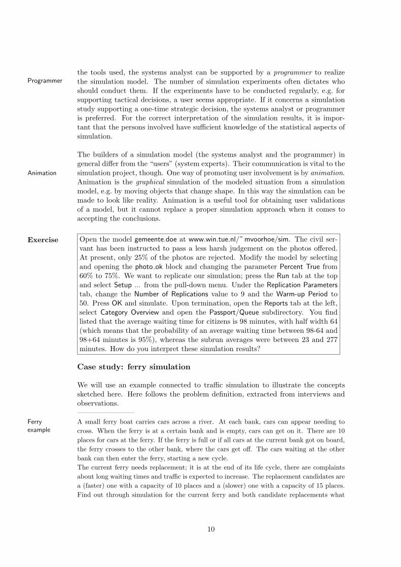
some extra feature is needed. Arena possesses a priority concept and this fits thebill perfectly. The getting off board transitions have the highest priority, followedPriority

by getting on board and finally setting sail. The ferry thus leaves when all possiblefirings of the getonboard transitions have occurred.Conceptual models can be verified by computing place invariants. Every resourceVerification

should correspond to a place invariant. Our ferry model indeed satisfies freeplace +Resourceinvariant crAB + crBA = 10 and atA + A2B + atB + B2A = 1. Also, deadlock-freedom can be

analyzed. If a conceptual model is not deadlock-free, the parameters (e.g. durations)Deadlockavoidance may prevent the deadlock from occurring, but it is dangerous to depend on them. By

adding places and arcs (i.e. by restricting the behavior) deadlocks can be avoided.

4.1.2 Photo example

We repeat the description of the model.A civil servant creates documents for citizens, who are queueing for his help. On average,a new citizen needing help arrives every 5 minutes. A photo must be attached to the doc-ument, which is judged by the servant. The judgement takes 1 minute on average. In 40%of the cases, the photo is judged inadequate, upon which the citizen is deferred to a nearbyphotographer to make a new one. This advice takes on average 1.5 minutes, after whichthe next citizen is helped. It takes on average 20 minutes to obtain a new photo; whenthe citizen returns with it, he gets priority for his document and the photo is immediatelyjudged correct. Making the document takes on average 3.5 minutes. The citizens complainabout excessive waiting times. The city hall management wants to solve the problem. Twosolutions are proposed:1. Every citizen should have his photo taken at the preferred shop.2. The judgement should be less harsh.The alternatives should be compared by simulation.

Here we have one case class (citizens), with different paths, depending on whether

14

the photo is accepted or not. The actions are entering, judgement, document-makingand (if the photo is rejected) instruction, making a new photo and returning. Theinitial table is as follows.

case action resource kindcitizen arrive - create

decide servant seizemake-doc servant releaseinstruct servant releasenew-photo -return servant seizeleave - dispose

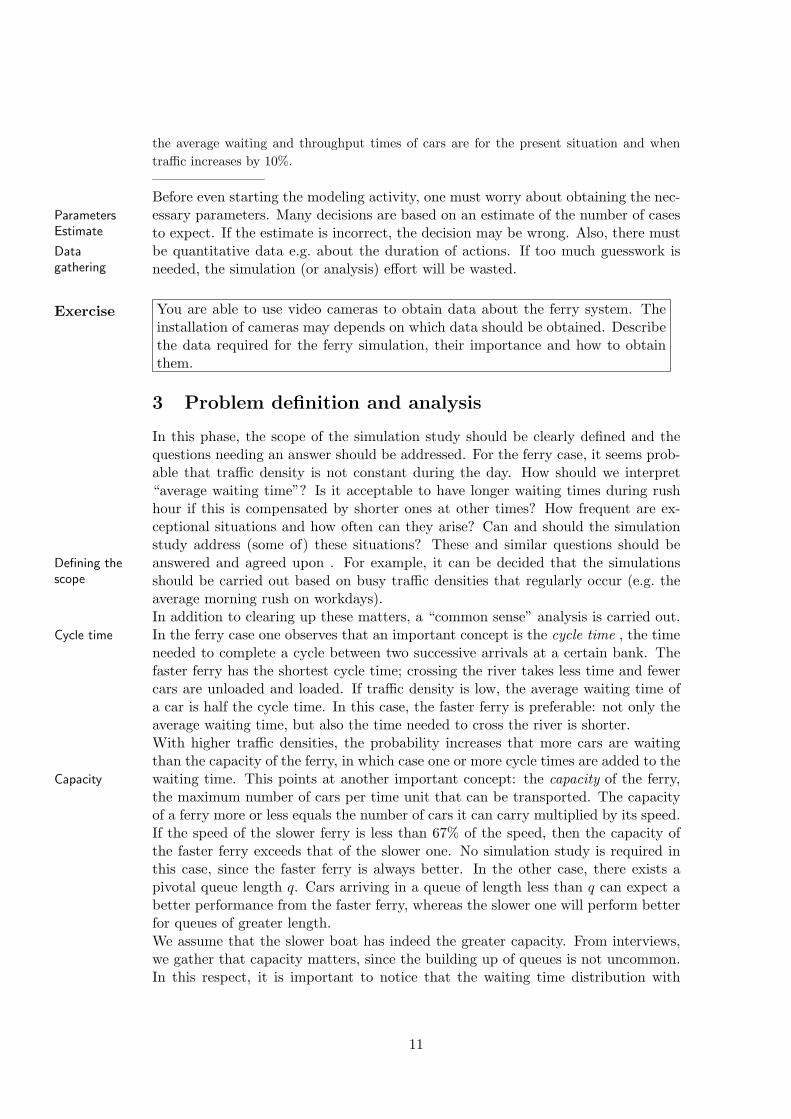
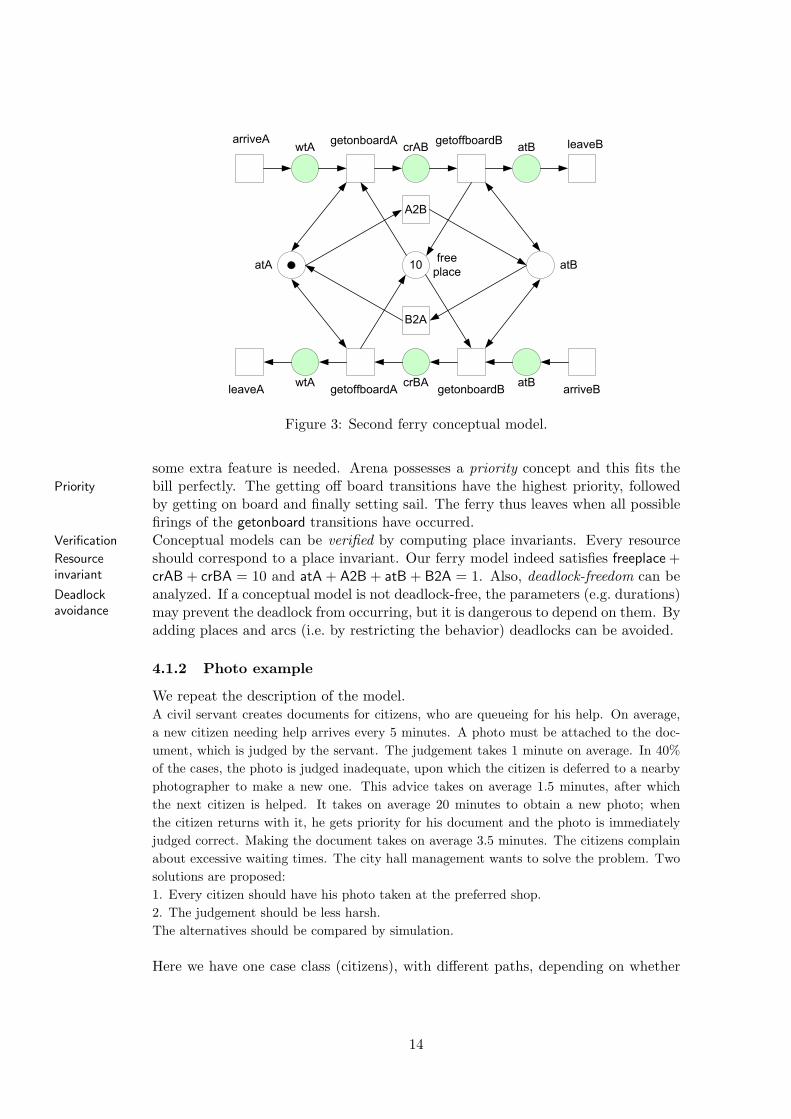
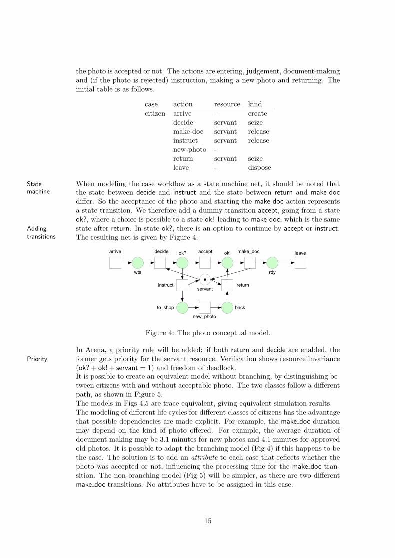
When modeling the case workflow as a state machine net, it should be noted thatStatemachine the state between decide and instruct and the state between return and make-doc

differ. So the acceptance of the photo and starting the make-doc action representsa state transition. We therefore add a dummy transition accept, going from a stateok?, where a choice is possible to a state ok! leading to make-doc, which is the samestate after return. In state ok?, there is an option to continue by accept or instruct.Adding

transitions The resulting net is given by Figure 4.

arrive decide make_doc leave

wts rdy

return

ok?

instruct

to_shop

ok!

new_photo

back

accept

servant

Figure 4: The photo conceptual model.

In Arena, a priority rule will be added: if both return and decide are enabled, theformer gets priority for the servant resource. Verification shows resource invariancePriority

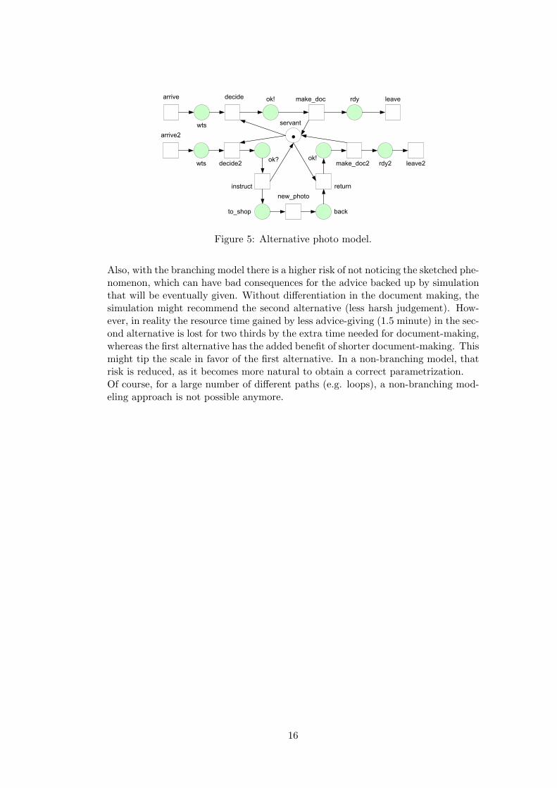
(ok? + ok! + servant = 1) and freedom of deadlock.It is possible to create an equivalent model without branching, by distinguishing be-tween citizens with and without acceptable photo. The two classes follow a differentpath, as shown in Figure 5.The models in Figs 4,5 are trace equivalent, giving equivalent simulation results.The modeling of different life cycles for different classes of citizens has the advantagethat possible dependencies are made explicit. For example, the make doc durationmay depend on the kind of photo offered. For example, the average duration ofdocument making may be 3.1 minutes for new photos and 4.1 minutes for approvedold photos. It is possible to adapt the branching model (Fig 4) if this happens to bethe case. The solution is to add an attribute to each case that reflects whether thephoto was accepted or not, influencing the processing time for the make doc tran-sition. The non-branching model (Fig 5) will be simpler, as there are two differentmake doc transitions. No attributes have to be assigned in this case.

15

arrive decide make_doc leave

wts

rdyok!

arrive2

decide2 make_doc2

servant

wtsok?

instruct

to_shop

ok!

new_photo

return

back

leave2rdy2

Figure 5: Alternative photo model.

Also, with the branching model there is a higher risk of not noticing the sketched phe-nomenon, which can have bad consequences for the advice backed up by simulationthat will be eventually given. Without differentiation in the document making, thesimulation might recommend the second alternative (less harsh judgement). How-ever, in reality the resource time gained by less advice-giving (1.5 minute) in the sec-ond alternative is lost for two thirds by the extra time needed for document-making,whereas the first alternative has the added benefit of shorter document-making. Thismight tip the scale in favor of the first alternative. In a non-branching model, thatrisk is reduced, as it becomes more natural to obtain a correct parametrization.Of course, for a large number of different paths (e.g. loops), a non-branching mod-eling approach is not possible anymore.

16

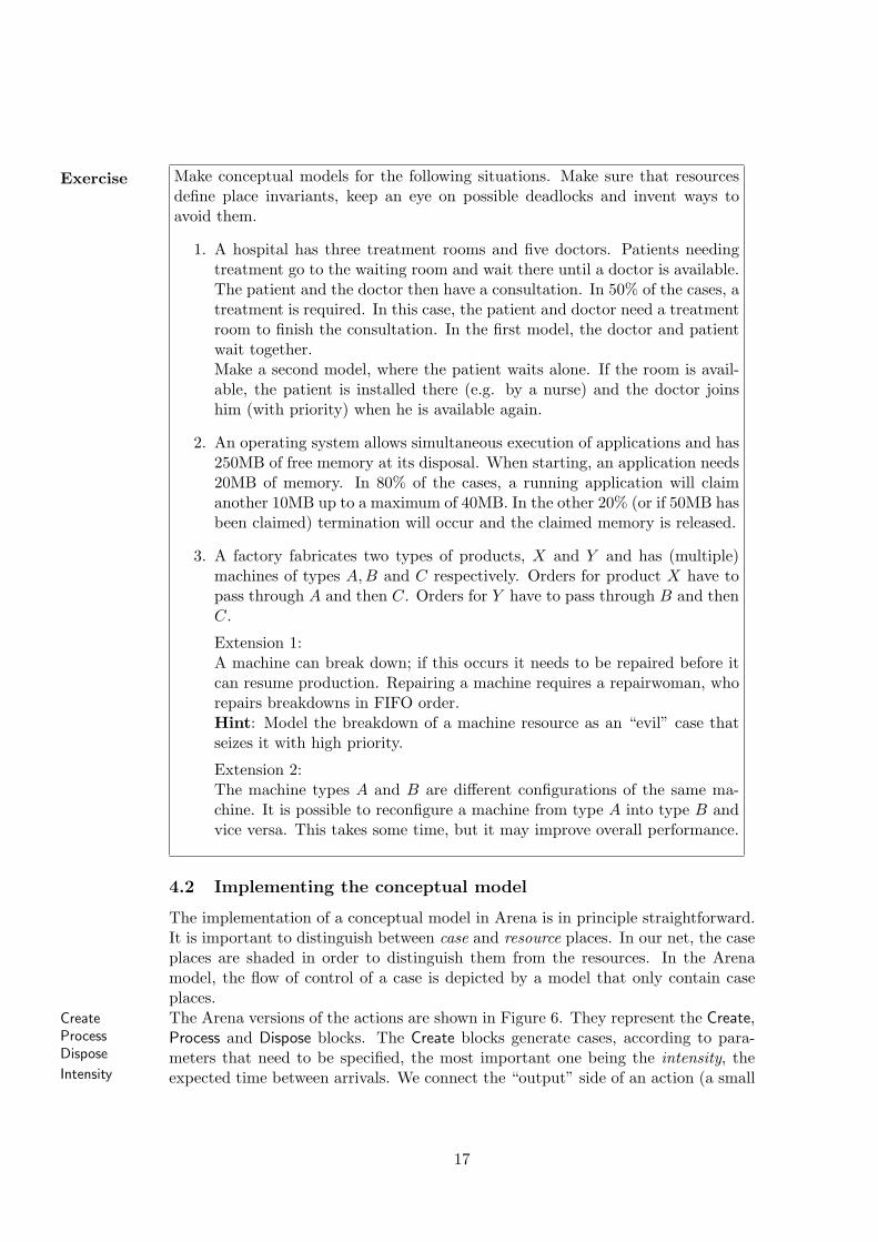
Exercise Make conceptual models for the following situations. Make sure that resourcesdefine place invariants, keep an eye on possible deadlocks and invent ways toavoid them.

1. A hospital has three treatment rooms and five doctors. Patients needingtreatment go to the waiting room and wait there until a doctor is available.The patient and the doctor then have a consultation. In 50% of the cases, atreatment is required. In this case, the patient and doctor need a treatmentroom to finish the consultation. In the first model, the doctor and patientwait together.Make a second model, where the patient waits alone. If the room is avail-able, the patient is installed there (e.g. by a nurse) and the doctor joinshim (with priority) when he is available again.

2. An operating system allows simultaneous execution of applications and has250MB of free memory at its disposal. When starting, an application needs20MB of memory. In 80% of the cases, a running application will claimanother 10MB up to a maximum of 40MB. In the other 20% (or if 50MB hasbeen claimed) termination will occur and the claimed memory is released.

3. A factory fabricates two types of products, X and Y and has (multiple)machines of types A,B and C respectively. Orders for product X have topass through A and then C. Orders for Y have to pass through B and thenC.

Extension 1:A machine can break down; if this occurs it needs to be repaired before itcan resume production. Repairing a machine requires a repairwoman, whorepairs breakdowns in FIFO order.Hint: Model the breakdown of a machine resource as an “evil” case thatseizes it with high priority.

Extension 2:The machine types A and B are different configurations of the same ma-chine. It is possible to reconfigure a machine from type A into type B andvice versa. This takes some time, but it may improve overall performance.

4.2 Implementing the conceptual model

The implementation of a conceptual model in Arena is in principle straightforward.It is important to distinguish between case and resource places. In our net, the caseplaces are shaded in order to distinguish them from the resources. In the Arenamodel, the flow of control of a case is depicted by a model that only contain caseplaces.The Arena versions of the actions are shown in Figure 6. They represent the Create,Create

ProcessDispose

Process and Dispose blocks. The Create blocks generate cases, according to para-meters that need to be specified, the most important one being the intensity, the

Intensity expected time between arrivals. We connect the “output” side of an action (a small

17

Create Process Dispose

Figure 6: Simple Arena building blocks.

black triangle) with the “input” side of its successor (a square). The Arena flow ofcontrol is left-to-right, which replaces the arrowheads. The Process blocks possess aduration parameter and parameters w.r.t. their resource behavior. These blocks arethe most frequently used. Some models (where all cases follow the same path) canbe fully modeled by them.

4.2.1 Ferry example

The conversion of the ferry model in Figure 2 is rather straightforward.

arriveA getonboardA getoffB leaveB

arriveB getonboardB getoffA leaveA

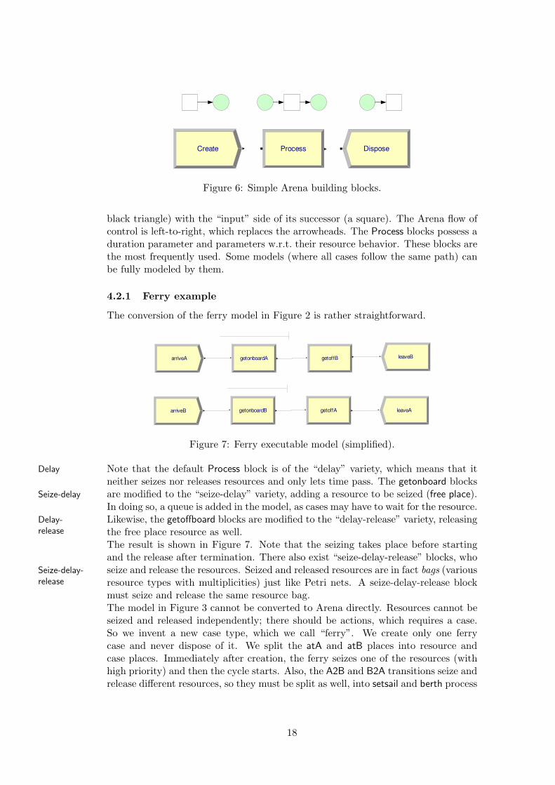
Figure 7: Ferry executable model (simplified).

Note that the default Process block is of the “delay” variety, which means that itDelay

neither seizes nor releases resources and only lets time pass. The getonboard blocksare modified to the “seize-delay” variety, adding a resource to be seized (free place).Seize-delay

In doing so, a queue is added in the model, as cases may have to wait for the resource.Likewise, the getoffboard blocks are modified to the “delay-release” variety, releasingDelay-

release the free place resource as well.The result is shown in Figure 7. Note that the seizing takes place before startingand the release after termination. There also exist “seize-delay-release” blocks, whoseize and release the resources. Seized and released resources are in fact bags (variousSeize-delay-

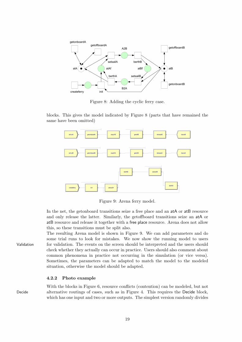
release resource types with multiplicities) just like Petri nets. A seize-delay-release blockmust seize and release the same resource bag.The model in Figure 3 cannot be converted to Arena directly. Resources cannot beseized and released independently; there should be actions, which requires a case.So we invent a new case type, which we call “ferry”. We create only one ferrycase and never dispose of it. We split the atA and atB places into resource andcase places. Immediately after creation, the ferry seizes one of the resources (withhigh priority) and then the cycle starts. Also, the A2B and B2A transitions seize andrelease different resources, so they must be split as well, into setsail and berth process

18

getonboardA

getoffboardAgetoffboardB

getonboardB

atA atB

A2B

setsailA berthB

setsailBberthA

B2A

atAf atBf

createferry init

Figure 8: Adding the cyclic ferry case.

blocks. This gives the model indicated by Figure 8 (parts that have remained thesame have been omitted)

arriveA stayABgetonboardA getoffB releaseB leaveB

arriveB stayBAgetonboardB getoffA releaseA leaveA

createferry setsailA

berthB setsailB

berthA

init

Figure 9: Arena ferry model.

In the net, the getonboard transitions seize a free place and an atA or atB resourceand only release the latter. Similarly, the getoffboard transitions seize an atA oratB resource and release it together with a free place resource. Arena does not allowthis, so these transitions must be split also.The resulting Arena model is shown in Figure 9. We can add parameters and dosome trial runs to look for mistakes. We now show the running model to usersfor validation. The events on the screen should be interpreted and the users shouldValidation

check whether they actually can occur in practice. Users should also comment aboutcommon phenomena in practice not occurring in the simulation (or vice versa).Sometimes, the parameters can be adapted to match the model to the modeledsituation, otherwise the model should be adapted.

4.2.2 Photo example

With the blocks in Figure 6, resource conflicts (contention) can be modeled, but notalternative routings of cases, such as in Figure 4. This requires the Decide block,Decide

which has one input and two or more outputs. The simplest version randomly divides

19

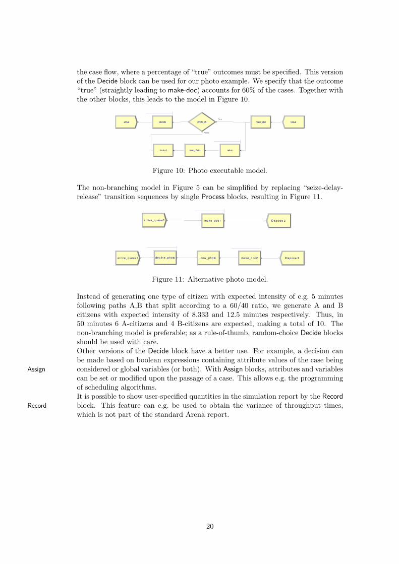
the case flow, where a percentage of “true” outcomes must be specified. This versionof the Decide block can be used for our photo example. We specify that the outcome“true” (straightly leading to make-doc) accounts for 60% of the cases. Together withthe other blocks, this leads to the model in Figure 10.

arrive decide leavephoto_ok

Tru e

Fa l s e

instruct

make_doc

new_photo return

Figure 10: Photo executable model.

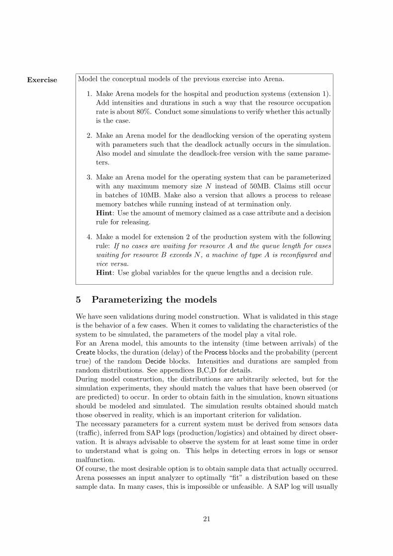
The non-branching model in Figure 5 can be simplified by replacing “seize-delay-release” transition sequences by single Process blocks, resulting in Figure 11.

arr iv e_queue1 D is pos e 2mak e_doc 1

new _photo D is pos e 3arr iv e_queue2 dec line_photo mak e_doc 2

Figure 11: Alternative photo model.

Instead of generating one type of citizen with expected intensity of e.g. 5 minutesfollowing paths A,B that split according to a 60/40 ratio, we generate A and Bcitizens with expected intensity of 8.333 and 12.5 minutes respectively. Thus, in50 minutes 6 A-citizens and 4 B-citizens are expected, making a total of 10. Thenon-branching model is preferable; as a rule-of-thumb, random-choice Decide blocksshould be used with care.Other versions of the Decide block have a better use. For example, a decision canbe made based on boolean expressions containing attribute values of the case beingconsidered or global variables (or both). With Assign blocks, attributes and variablesAssign

can be set or modified upon the passage of a case. This allows e.g. the programmingof scheduling algorithms.It is possible to show user-specified quantities in the simulation report by the Recordblock. This feature can e.g. be used to obtain the variance of throughput times,Record

which is not part of the standard Arena report.

20

Exercise Model the conceptual models of the previous exercise into Arena.

1. Make Arena models for the hospital and production systems (extension 1).Add intensities and durations in such a way that the resource occupationrate is about 80%. Conduct some simulations to verify whether this actuallyis the case.

2. Make an Arena model for the deadlocking version of the operating systemwith parameters such that the deadlock actually occurs in the simulation.Also model and simulate the deadlock-free version with the same parame-ters.

3. Make an Arena model for the operating system that can be parameterizedwith any maximum memory size N instead of 50MB. Claims still occurin batches of 10MB. Make also a version that allows a process to releasememory batches while running instead of at termination only.Hint: Use the amount of memory claimed as a case attribute and a decisionrule for releasing.

4. Make a model for extension 2 of the production system with the followingrule: If no cases are waiting for resource A and the queue length for caseswaiting for resource B exceeds N , a machine of type A is reconfigured andvice versa.Hint: Use global variables for the queue lengths and a decision rule.

5 Parameterizing the models

We have seen validations during model construction. What is validated in this stageis the behavior of a few cases. When it comes to validating the characteristics of thesystem to be simulated, the parameters of the model play a vital role.For an Arena model, this amounts to the intensity (time between arrivals) of theCreate blocks, the duration (delay) of the Process blocks and the probability (percenttrue) of the random Decide blocks. Intensities and durations are sampled fromrandom distributions. See appendices B,C,D for details.During model construction, the distributions are arbitrarily selected, but for thesimulation experiments, they should match the values that have been observed (orare predicted) to occur. In order to obtain faith in the simulation, known situationsshould be modeled and simulated. The simulation results obtained should matchthose observed in reality, which is an important criterion for validation.The necessary parameters for a current system must be derived from sensors data(traffic), inferred from SAP logs (production/logistics) and obtained by direct obser-vation. It is always advisable to observe the system for at least some time in orderto understand what is going on. This helps in detecting errors in logs or sensormalfunction.Of course, the most desirable option is to obtain sample data that actually occurred.Arena possesses an input analyzer to optimally “fit” a distribution based on thesesample data. In many cases, this is impossible or unfeasible. A SAP log will usually

21

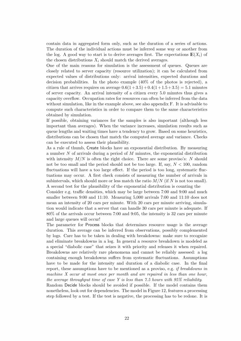
contain data in aggregated form only, such as the duration of a series of actions.The duration of the individual actions must be inferred some way or another fromthe log. A good way to start is to derive averages first. The expectations IE(Xi) ofthe chosen distributions Xi should match the derived averages.One of the main reasons for simulation is the assessment of queues. Queues areclosely related to server capacity (resource utilization); it can be calculated fromexpected values of distributions only: arrival intensities, expected durations anddecision probabilities. In the photo example (40% of the photos is rejected), acitizen that arrives requires on average 0.6(1+3.5)+0.4(1+1.5+3.5) = 5.1 minutesof server capacity. An arrival intensity of a citizen every 5.0 minutes thus gives acapacity overflow. Occupation rates for resources can often be inferred from the datawithout simulation, like in the example above, see also appendix F. It is advisable tocompute such characteristics in order to compare them to the same characteristicsobtained by simulation.If possible, obtaining variances for the samples is also important (although lessimportant than averages). When the variance increases, simulation results such asqueue lengths and waiting times have a tendency to grow. Based on some heuristics,distributions can be chosen that match the computed average and variance. Checkscan be executed to assess their plausibility.As a rule of thumb, Create blocks have an exponential distribution. By measuringa number N of arrivals during a period of M minutes, the exponential distributionwith intensity M/N is often the right choice. There are some proviso’s: N shouldnot be too small and the period should not be too large. If, say, N < 100, randomfluctuations will have a too large effect. If the period is too long, systematic fluc-tuations may occur. A first check consists of measuring the number of arrivals insubintervals, which should more or less match the ratio M/N (if N is not too small).A second test for the plausibility of the exponential distribution is counting theConsider e.g. traffic densities, which may be large between 7:00 and 9:00 and muchsmaller between 9:00 and 11:10. Measuring 5,000 arrivals 7:00 and 11:10 does notmean an intensity of 20 cars per minute. With 20 cars per minute arriving, simula-tion would indicate that a server that can handle 30 cars per minute is adequate. If80% of the arrivals occur between 7:00 and 9:05, the intensity is 32 cars per minuteand large queues will occur!The parameter for Process blocks that determines resource usage is the averageduration. This average can be inferred from observations, possibly complementedby logs. Care has to be taken in dealing with breakdowns: make sure to recognizeand eliminate breakdowns in a log. In general a resource breakdown is modeled asa special “diabolic case” that seizes it with priority and releases it when repaired.Breakdowns are relatively rare phenomena and cannot be reliably assessed: a logcontaining enough breakdowns suffers from systematic fluctuations. Assumptionshave to be made for the intensity and duration of a diabolic case. In the finalreport, these assumptions have to be mentioned as a proviso, e.g. if breakdowns inmachine X occur at most once per month and are repaired in less than one hour,the average throughput time of case Y is less than 7.5 hours with 95% reliability.Random Decide blocks should be avoided if possible. If the model contains themnonetheless, look out for dependencies. The model in Figure 12, features a processingstep followed by a test. If the test is negative, the processing has to be redone. It is

22

Create Process

True

False

Decide Dispose

Figure 12: Iterative model.

possible that the various iterations (first, second, ...) possess different characteristics.For example, the average processing step may take on average 1.56 hours and 77% ofthe tests is positive. By closer inspection, the duration of the processing depends onthe iteration number: the first processing step takes on average 1.7 hours and 70%of the tests is positive. In the remaining 30%, the second processing step takes onaverage 1.1 hours and 99% of the tests are positive. The third iteration has a shortduration; all tests following it have been positive in the log studied. The averageresource utilization is the same in both models, but the expected waiting time ishigher in reality than a simulation from the above model would indicate.Analyzing the measured data, consulting the users and keeping one’s eyes open areall necessary to get a proper parametrization. A necessary validation (if possible) isto make a parameterized model of the current system, simulate it and check whetherthe simulation results (such as queue lengths, waiting times and resource utilization)match the actual results measured. Any mismatch should be investigated, explainedand corrected.In the ferry example, we installed video cameras to record the events. From therecorded data, we want to infer the arrival processes and the duration of the ferrycrossing and getting on and off board. A problem that often occurs is that arrivalintensities are not constant. If the ferry is heavily used for commuter traffic, higherintensities occur during workdays around 8am and 5pm. If the ferry is mainly usedfor leisure rides, intensities are higher during holidays with nice weather conditions.Together with the user, some representative periods must be selected. For theseperiods, the arrival times should be derived from the recorded images. The crossingtime may be influenced by weather circumstances (wind, current) and the passingof other boats on the river. Here also, selecting representative periods may be nec-essary. Getting off and on board requires some preparations, that can be discountedin the crossing, followed by an amount of time proportional to the number of carsthat get off and on board.Obtaining the necessary data from the recordings requires some man-hours of te-dious, yet important work. Fortunately, it is not necessary to look at the videorecording in “real time”. The video recording should display the time, so that wecan use the “fast-forward” functionality, obtaining a trace of several hours, startingas shown.

time event06:59:57 A2B cars enter07:00:07 4 cars entered07:00:19 leave dock A07:03:56 arrive at dock B07:04:08 A2B cars leave

23

07:04:15 4 cars left07:04:21 B2A cars enter07:04:29 5 cars entered07:04:36 leave dock B...

From this information, parameters can be inferred. The Arena input analyzer canhelp in this respect. It is not always possible to parameterize by “standard” distri-butions. Examples are traffic light simulations (occurrence of “bursts”) or machinebreakdowns (two “breakdown classes” with different characteristics). Observing theprocess, noting comments and careful validation can help to avoid mistakes.

Exercise 1. Indicate how the parameters of the ferry model can be inferred from the atrace such as shown above.2. A production plant possesses a breakdown-prone machine resource. The oc-currence and duration of breakdowns in 2006 have been recorded, giving thefollowing pattern.from 0 3 6 9 12 15 18 21 24 27 30to 3 6 9 12 15 18 21 24 27 30 ∞amount 3 11 8 5 3 2 4 3 2 2 4

How do you model the breakdowns. What kind of distribution you choose?

6 Processing the results

Simulation is used to support decisions, such as the number of resources of a certaintype that has to be installed in order to guarantee a certain service level. Forexample, we want to guarantee that incoming telephone calls are answered within20 seconds on average and that at least 90% of the calls is answered in less than 30seconds. By simulation, it can be assessed for given combinations of infrastructure,procedures and available personnel whether this requirement can be met. It is veryimportant to adequately report the extent of the statements made.

6.1 Observed quantities

During simulation, repeated observations are made of quantities such as waitingObservations times, run times, processing times or stock levels. Also, occurrences of certain

events can be counted. Individual observations have little interest. Instead, weare interested in statistical data about the observed quantities, such as means andvariances.Suppose we have k consecutive observations, called x1, x2, ...xk. These observationsare also called a random sample. The mean of a number of observations is also calledthe sample mean. We denote the sample mean of x1, x2, ...xk as x:Sample

mean

x =∑k

i=1 xi

k

Please note that the sample mean is an estimate of the true mean.The variance of a number of observations is also called the sample variance. ThisSample

variance

24

variance is a measure for the deviation from the mean. The smaller the variance,the closer the observations will be to the mean. We can find the sample variance s2

by using the following formula:

s2 =∑k

i=1(xi − x)2

k − 1

We can rewrite this formula as:

s2 =(∑k

i=1 xi2)− 1

k

(∑ki=1 xi

)2

k − 1

During a simulation, Arena keeps track of the number of observations k, the sumof all observations

∑ki=1 xi and the sum of the squares of all observations

∑ki=1 xi

2.In doing so, the sample mean and the sample variance can be obtained. The squareroot of the sample variance s =

√s2 is also called the sample standard deviation.Sample

standarddeviation

Apart for the mean and the variance of a random sample, there is also the so-calledmedian of k observations x1, x2, . . . , xk. The median is the value of the observation

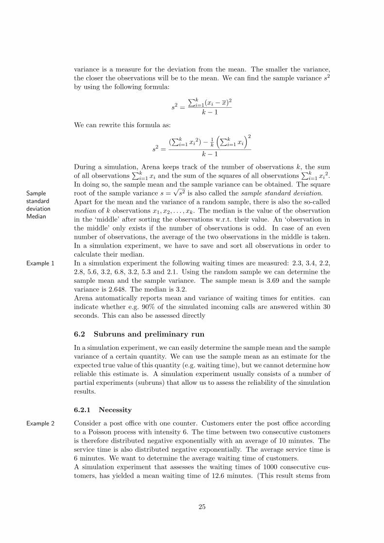
Median in the ‘middle’ after sorting the observations w.r.t. their value. An ‘observation inthe middle’ only exists if the number of observations is odd. In case of an evennumber of observations, the average of the two observations in the middle is taken.In a simulation experiment, we have to save and sort all observations in order tocalculate their median.In a simulation experiment the following waiting times are measured: 2.3, 3.4, 2.2,Example 1

2.8, 5.6, 3.2, 6.8, 3.2, 5.3 and 2.1. Using the random sample we can determine thesample mean and the sample variance. The sample mean is 3.69 and the samplevariance is 2.648. The median is 3.2.Arena automatically reports mean and variance of waiting times for entities. canindicate whether e.g. 90% of the simulated incoming calls are answered within 30seconds. This can also be assessed directly

6.2 Subruns and preliminary run

In a simulation experiment, we can easily determine the sample mean and the samplevariance of a certain quantity. We can use the sample mean as an estimate for theexpected true value of this quantity (e.g. waiting time), but we cannot determine howreliable this estimate is. A simulation experiment usually consists of a number ofpartial experiments (subruns) that allow us to assess the reliability of the simulationresults.

6.2.1 Necessity

Consider a post office with one counter. Customers enter the post office accordingExample 2

to a Poisson process with intensity 6. The time between two consecutive customersis therefore distributed negative exponentially with an average of 10 minutes. Theservice time is also distributed negative exponentially. The average service time is6 minutes. We want to determine the average waiting time of customers.A simulation experiment that assesses the waiting times of 1000 consecutive cus-tomers, has yielded a mean waiting time of 12.6 minutes. (This result stems from

25

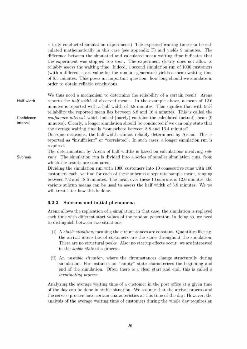
a truly conducted simulation experiment!) The expected waiting time can be cal-culated mathematically in this case (see appendix F) and yields 9 minutes. Thedifference between the simulated and calculated mean waiting time indicates thatthe experiment was stopped too soon. The experiment clearly does not allow toreliably assess the waiting time. Indeed, a second simulation run of 1000 customers(with a different start value for the random generator) yields a mean waiting timeof 8.5 minutes. This poses an important question: how long should we simulate inorder to obtain reliable conclusions.

We thus need a mechanism to determine the reliability of a certain result. Arenareports the half width of observed means. In the example above, a mean of 12.6Half width

minutes is reported with a half width of 3.8 minutes. This signifies that with 95%reliability the reported mean lies between 8.8 and 16.4 minutes. This is called theconfidence interval, which indeed (barely) contains the calculated (actual) mean (9Confidence

interval minutes). Clearly, a longer simulation should be conducted if we can only state thatthe average waiting time is “somewhere between 8.8 and 16.4 minutes”.On some occasions, the half width cannot reliably determined by Arena. This isreported as “insufficient” or “correlated”. In such cases, a longer simulation run isrequired.The determination by Arena of half widths is based on calculations involving sub-runs. The simulation run is divided into a series of smaller simulation runs, fromSubruns

which the results are compared.Dividing the simulation run with 1000 customers into 10 consecutive runs with 100customers each, we find for each of these subruns a separate sample mean, rangingbetween 7.2 and 18.6 minutes. The mean over these 10 subruns is 12.6 minutes; thevarious subrun means can be used to assess the half width of 3.8 minutes. We wewill treat later how this is done.

6.2.2 Subruns and initial phenomena

Arena allows the replication of a simulation; in that case, the simulation is replayedeach time with different start values of the random generator. In doing so, we needto distinguish between two situations:

(i) A stable situation, meaning the circumstances are constant. Quantities like e.g.the arrival intensities of customers are the same throughout the simulation.There are no structural peaks. Also, no startup effects occur: we are interestedin the stable state of a process.

(ii) An unstable situation, where the circumstances change structurally duringsimulation. For instance, an “empty” state characterizes the beginning andend of the simulation. Often there is a clear start and end; this is called aterminating process.

Analyzing the average waiting time of a customer in the post office at a given timeof the day can be done in stable situation. We assume that the arrival process andthe service process have certain characteristics at this time of the day. However, theanalysis of the average waiting time of customers during the whole day requires an

26

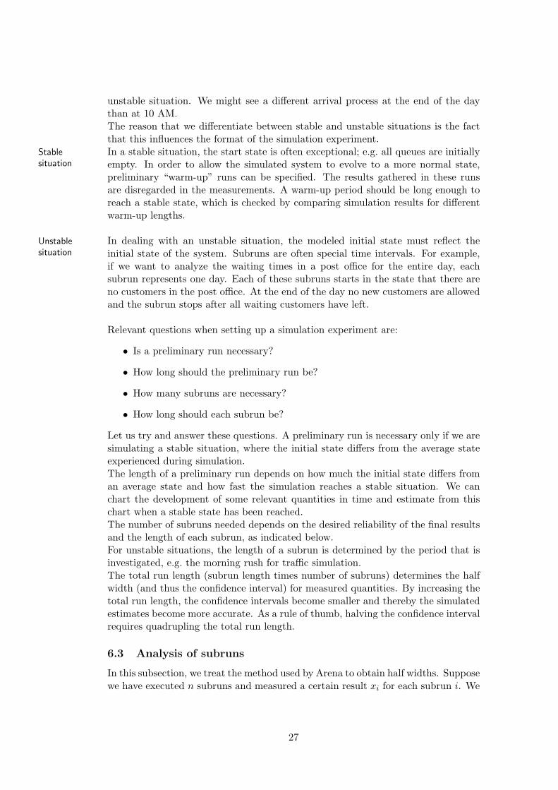
unstable situation. We might see a different arrival process at the end of the daythan at 10 AM.The reason that we differentiate between stable and unstable situations is the factthat this influences the format of the simulation experiment.In a stable situation, the start state is often exceptional; e.g. all queues are initiallyStable

situation empty. In order to allow the simulated system to evolve to a more normal state,preliminary “warm-up” runs can be specified. The results gathered in these runsare disregarded in the measurements. A warm-up period should be long enough toreach a stable state, which is checked by comparing simulation results for differentwarm-up lengths.

In dealing with an unstable situation, the modeled initial state must reflect theUnstablesituation initial state of the system. Subruns are often special time intervals. For example,

if we want to analyze the waiting times in a post office for the entire day, eachsubrun represents one day. Each of these subruns starts in the state that there areno customers in the post office. At the end of the day no new customers are allowedand the subrun stops after all waiting customers have left.

Relevant questions when setting up a simulation experiment are:

• Is a preliminary run necessary?

• How long should the preliminary run be?

• How many subruns are necessary?

• How long should each subrun be?

Let us try and answer these questions. A preliminary run is necessary only if we aresimulating a stable situation, where the initial state differs from the average stateexperienced during simulation.The length of a preliminary run depends on how much the initial state differs froman average state and how fast the simulation reaches a stable situation. We canchart the development of some relevant quantities in time and estimate from thischart when a stable state has been reached.The number of subruns needed depends on the desired reliability of the final resultsand the length of each subrun, as indicated below.For unstable situations, the length of a subrun is determined by the period that isinvestigated, e.g. the morning rush for traffic simulation.The total run length (subrun length times number of subruns) determines the halfwidth (and thus the confidence interval) for measured quantities. By increasing thetotal run length, the confidence intervals become smaller and thereby the simulatedestimates become more accurate. As a rule of thumb, halving the confidence intervalrequires quadrupling the total run length.

6.3 Analysis of subruns

In this subsection, we treat the method used by Arena to obtain half widths. Supposewe have executed n subruns and measured a certain result xi for each subrun i. We

27

know there exists a “true” value (called µ) that each xi approximates and we wantto derive assertions about µ from the xi. For example, xi is the mean waiting timemeasured in subrun i and µ the “true” mean waiting time that we could find byconducting a hypothetical simulation experiment of infinite length. (Instead, wemight consider the mean variance of the waiting time, the mean occupation rate ofa server or the mean length of a queue.) We must be certain that the values xi

are mutually independent for all subruns. If Arena discovers dependencies, the halfwidth is reported as “correlated”. Given the results x1, x2, . . . , xn, we derive thesample mean x:

x =∑n

i=1 xi

n

and the sample variance s2:

s2 =∑n

i=1(xi − x)2

n− 1

Note that the sample mean and the sample variance for the results of the varioussubruns should not be confused with the mean and the variance of a number ofmeasures within one subrun! We can consider x as an estimate of µ. The value xcan be seen as a sample from a random variable X called estimator. The value 1

s√n

is an indication of the reliability of the estimate x. If s√n

is small, it is a goodestimate.

6.3.1 The situation with over 30 subruns

If there is a large number of subruns, we can consider the estimator X (becauseof the central limit theorem) as normally distributed. We will therefore treat thesituation with over 30 subruns as a special case.

The fact that s√n

measures how well x approximates µ, allows us to determine theWhen dowe stopgeneratingsubruns?

time that we can stop generating subruns.

(i) Choose a value d for the permitted standard deviation from the estimatedvalue x.

(ii) Generate at least 30 subruns and note per subrun the value xi.

(iii) Generate additional subruns until s√n≤ d, where s is the sample standard

deviation and n the number of subruns executed.

(iv) The sample mean x is now an estimate of the quantity to be studied.

There are two other reasons why in this case at least 30 subruns have to be executed.In the first place, X is only approximately normally distributed with a large numberof subruns. This is a compelling reason to make sure that there are at least 30mutually independent subruns. Another reason for choosing an adequate number

1The variance of the estimator X is Var[x] = Var[ 1n

Pni=1 xi] = σ2

n. The standard deviation of

x thus equals σ√n. As s is a good estimate of σ, the amount s√

nyields a good estimate for the

standard deviation of x.

28

of subruns is the fact that by increasing the number of subruns, s becomes a betterestimate of the true standard deviation.

Given a large number of independent subruns, we can also determine a confidenceinterval for the quantity to be studied. Because x is the average of a large number ofConfidence

interval independent measures, we can assume that x is approximately normally distributed.(Central Limit Theorem, Appendix E). From this fact, we deduce the probabilitythat µ lies within a so-called confidence interval. Given the sample mean x and thesample standard deviation s, the true value µ conforms with confidence (1 − α) tothe following equation:

x− s√n

z(α

2) < µ < x +

s√n

z(α

2)

where z(α2 ) is defined as follows. If Z is a standard normally distributed random

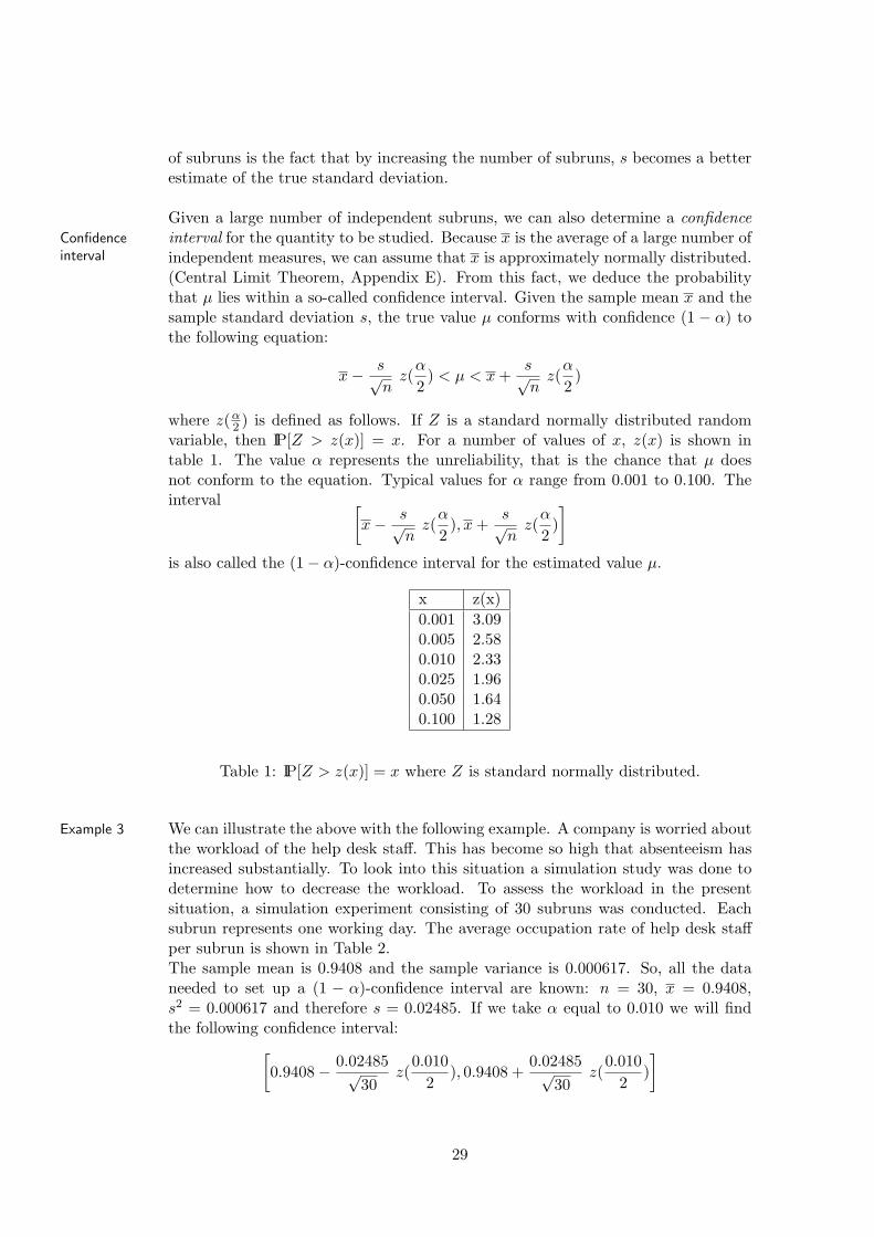
variable, then IP[Z > z(x)] = x. For a number of values of x, z(x) is shown intable 1. The value α represents the unreliability, that is the chance that µ doesnot conform to the equation. Typical values for α range from 0.001 to 0.100. Theinterval [

x− s√n

z(α

2), x +

s√n

z(α

2)]

is also called the (1− α)-confidence interval for the estimated value µ.

x z(x)0.001 3.090.005 2.580.010 2.330.025 1.960.050 1.640.100 1.28

Table 1: IP[Z > z(x)] = x where Z is standard normally distributed.

We can illustrate the above with the following example. A company is worried aboutExample 3

the workload of the help desk staff. This has become so high that absenteeism hasincreased substantially. To look into this situation a simulation study was done todetermine how to decrease the workload. To assess the workload in the presentsituation, a simulation experiment consisting of 30 subruns was conducted. Eachsubrun represents one working day. The average occupation rate of help desk staffper subrun is shown in Table 2.The sample mean is 0.9408 and the sample variance is 0.000617. So, all the dataneeded to set up a (1 − α)-confidence interval are known: n = 30, x = 0.9408,s2 = 0.000617 and therefore s = 0.02485. If we take α equal to 0.010 we will findthe following confidence interval:

[0.9408− 0.02485√

30z(

0.0102

), 0.9408 +0.02485√

30z(

0.0102

)]

29

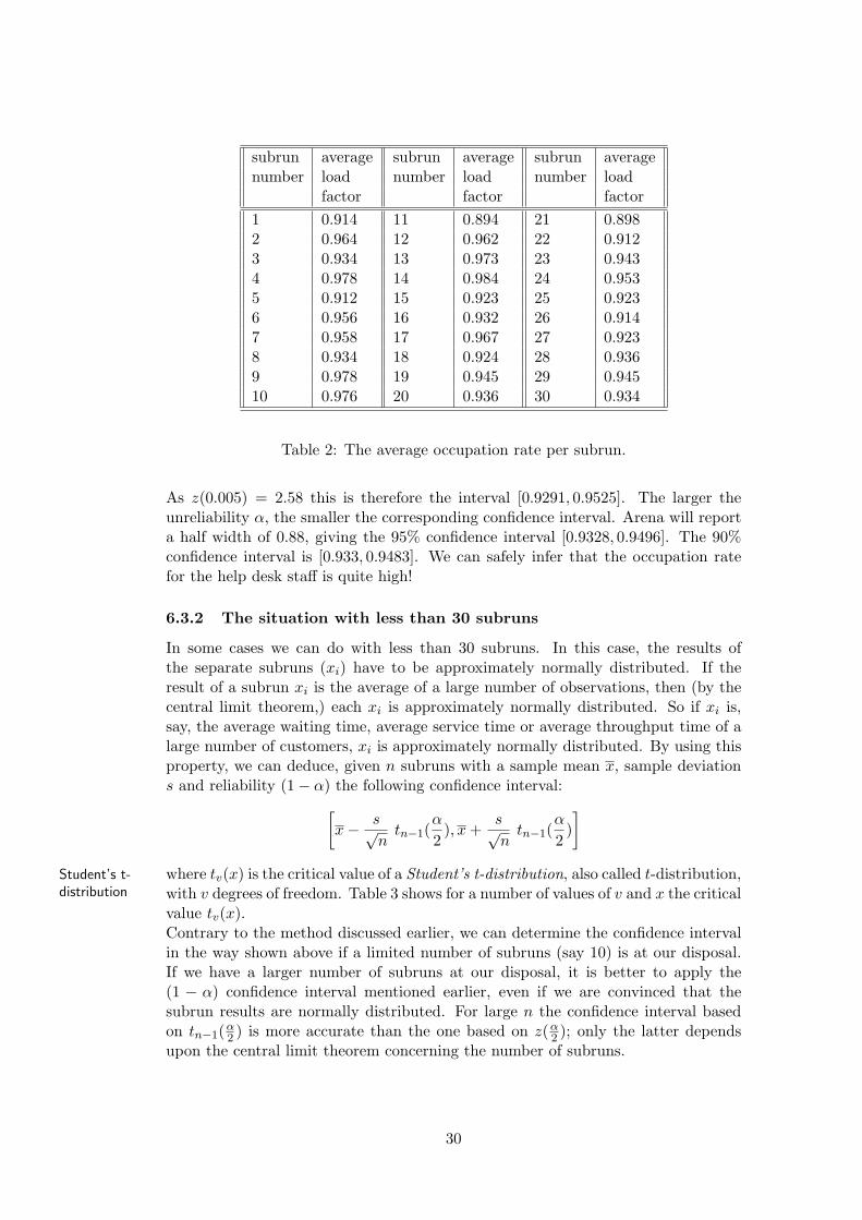
subrun average subrun average subrun averagenumber load number load number load

factor factor factor1 0.914 11 0.894 21 0.8982 0.964 12 0.962 22 0.9123 0.934 13 0.973 23 0.9434 0.978 14 0.984 24 0.9535 0.912 15 0.923 25 0.9236 0.956 16 0.932 26 0.9147 0.958 17 0.967 27 0.9238 0.934 18 0.924 28 0.9369 0.978 19 0.945 29 0.94510 0.976 20 0.936 30 0.934

Table 2: The average occupation rate per subrun.

As z(0.005) = 2.58 this is therefore the interval [0.9291, 0.9525]. The larger theunreliability α, the smaller the corresponding confidence interval. Arena will reporta half width of 0.88, giving the 95% confidence interval [0.9328, 0.9496]. The 90%confidence interval is [0.933, 0.9483]. We can safely infer that the occupation ratefor the help desk staff is quite high!

6.3.2 The situation with less than 30 subruns

In some cases we can do with less than 30 subruns. In this case, the results ofthe separate subruns (xi) have to be approximately normally distributed. If theresult of a subrun xi is the average of a large number of observations, then (by thecentral limit theorem,) each xi is approximately normally distributed. So if xi is,say, the average waiting time, average service time or average throughput time of alarge number of customers, xi is approximately normally distributed. By using thisproperty, we can deduce, given n subruns with a sample mean x, sample deviations and reliability (1− α) the following confidence interval:

[x− s√

ntn−1(

α

2), x +

s√n

tn−1(α

2)]

where tv(x) is the critical value of a Student’s t-distribution, also called t-distribution,Student’s t-distribution with v degrees of freedom. Table 3 shows for a number of values of v and x the critical

value tv(x).Contrary to the method discussed earlier, we can determine the confidence intervalin the way shown above if a limited number of subruns (say 10) is at our disposal.If we have a larger number of subruns at our disposal, it is better to apply the(1 − α) confidence interval mentioned earlier, even if we are convinced that thesubrun results are normally distributed. For large n the confidence interval basedon tn−1(α

2 ) is more accurate than the one based on z(α2 ); only the latter depends

upon the central limit theorem concerning the number of subruns.

30

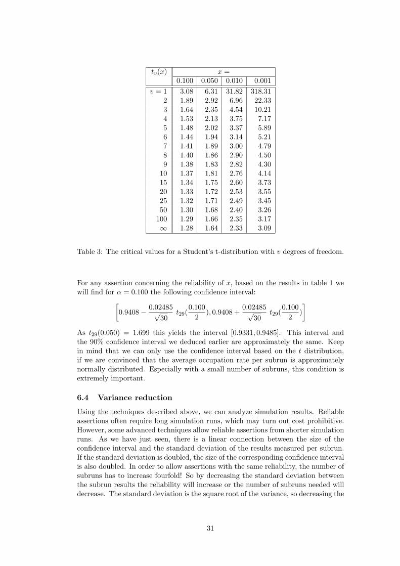
tv(x) x =0.100 0.050 0.010 0.001

v = 1 3.08 6.31 31.82 318.312 1.89 2.92 6.96 22.333 1.64 2.35 4.54 10.214 1.53 2.13 3.75 7.175 1.48 2.02 3.37 5.896 1.44 1.94 3.14 5.217 1.41 1.89 3.00 4.798 1.40 1.86 2.90 4.509 1.38 1.83 2.82 4.30

10 1.37 1.81 2.76 4.1415 1.34 1.75 2.60 3.7320 1.33 1.72 2.53 3.5525 1.32 1.71 2.49 3.4550 1.30 1.68 2.40 3.26

100 1.29 1.66 2.35 3.17∞ 1.28 1.64 2.33 3.09

Table 3: The critical values for a Student’s t-distribution with v degrees of freedom.

For any assertion concerning the reliability of x, based on the results in table 1 wewill find for α = 0.100 the following confidence interval:

[0.9408− 0.02485√

30t29(

0.1002

), 0.9408 +0.02485√

30t29(

0.1002

)]

As t29(0.050) = 1.699 this yields the interval [0.9331, 0.9485]. This interval andthe 90% confidence interval we deduced earlier are approximately the same. Keepin mind that we can only use the confidence interval based on the t distribution,if we are convinced that the average occupation rate per subrun is approximatelynormally distributed. Especially with a small number of subruns, this condition isextremely important.

6.4 Variance reduction

Using the techniques described above, we can analyze simulation results. Reliableassertions often require long simulation runs, which may turn out cost prohibitive.However, some advanced techniques allow reliable assertions from shorter simulationruns. As we have just seen, there is a linear connection between the size of theconfidence interval and the standard deviation of the results measured per subrun.If the standard deviation is doubled, the size of the corresponding confidence intervalis also doubled. In order to allow assertions with the same reliability, the number ofsubruns has to increase fourfold! So by decreasing the standard deviation betweenthe subrun results the reliability will increase or the number of subruns needed willdecrease. The standard deviation is the square root of the variance, so decreasing the

31

variance and the standard deviation goes hand in hand. The techniques that focuson decreasing the variance are called variance reducing techniques Some well-knownVariance re-

ducingtechniques

techniques are:

• antithetic variates

• common random numbers

• control variates

• conditioning

• stratified sampling

• importance sampling

We will not explain all of these techniques at length and only summarize the firsttwo.

In a simulation experiment random numbers are constantly being used and assignedAntitheticvariates to random variables. A good random generator will generate numbers that are

independent of each other. It is, however, not necessary to generate a new setof random numbers for each subrun. If r1, r2, . . . , rn are random numbers, so are(1− r1), (1− r2), . . . , (1− rn)! These numbers are called antithetic. If we generatenew random numbers for each odd subrun and we use antithetic random numbers foreach even subrun, we only need half of the random numbers (if the total number ofsubruns is even). There is another bonus. The results for subrun 2k− 1 and subrun2k will probably be negatively correlated. If e.g. subrun 2k − 1 is characterized byfrequent arrivals (e.g. caused by sampling small random numbers), the arrivals insubrun 2k will be infrequent since antithetic, thus large numbers will be sampled.If x2k−1 and x2k represent the results of two consecutive subruns, in all probabilityCov[x2k−1, x2k] will be smaller than zero. This leads to a decrease in the varianceof the mean of x2k−1 and x2k, as:

Var[X + Y

2] =

14(Var[X] + Var[Y ] + 2Cov[X,Y ])

The total sample variance will then also decrease, narrowing down the confidenceinterval.

If one wants to compare two alternatives, it is intuitively obvious that the circum-Common ran-domnumbers

stances should be as similar as possible. This means that the samples taken in thesimulation runs of either alternative should correspond maximally. When simulatingdifferent arrangements of the post office, the alternatives may use the same randomnumbers for interim arrival times and service times. In this way the variance of thedifference between both alternatives may be substantially reduced.

There are various advanced techniques for increasing the information obtained throughsimulation. These techniques have to be used with great care. More details can befound in [2, 10, 11].

32

6.5 Sensitivity analysis

Given a certain model, one can give well-founded estimates for the expected waitingtimes, occupation rates, fault frequencies etc., by using subruns and calculatingconfidence intervals. Since these results are based on a specific situation, it is unclearhow sensitive they are. If we find an estimated average waiting time of 10 minutesSensitivity

for an arrival process with an average interarrival time of 5 minutes, what would theaverage waiting time be if the interarrival time is not 5 but 6 minutes? In generala model has a number of parameters; adjustable quantities, like average interarrivalModel

parameters time, average service time and average response time. For a simulation experimenteach of these quantities is given a certain value. This value is often estimated,as the exact value is unknown. Also the probability distribution chosen will onlyapproximate the true distribution of values. It is therefore of the utmost importanceto know how sensitive the results are to variations in the model parameters.

A sensitivity analysis is carried out to assess dependencies between the model pa-Sensitivityanalysis rameters and the results. To test the sensitivity, a number of experiments are con-

ducted with slight variations in parameter settings. These experiments indicate theextent to which slight variations can influence the final result. Adjusting the settingof a certain parameter will often only mildly influence on the final result. Some-times, however, a slight adjustment of a parameter will lead to completely differentresults. A resource with a high occupation rate will be more sensitive to fluctuationsin its arrival process than a resource with a lower occupation rate. We also use theterm robustness. A model is robust if slight deviations in parameter settings barelyinfluence the final result.

Exercise Assess the parameters used for the ferry simulation model given as example. As-sess their reliability and their stability over time and decide a sensitivity analysisrange for them. For example traffic densities have been obtained by collectingpast data. The amount of traffic is influenced by many factors and may verywell increase or decrease over time, so an extensive sensitivity analysis of theseparameters is needed.

7 Pitfalls

As already indicated in the introduction, simulation is often used to support criticalstrategic decisions, where errors are very expensive. However, errors are manifoldand often easily introduced when conducting a simulation study, so one has to beon the alert constantly. We will look at the phases in the life cycle of a simulationstudy and identify the dangers in each specific phase. Figure 13 shows the phasesof a simulation study and the possible sources of errors.Possible

errorsources

The problem definition can be inconsistent (contradictory) or incomplete (vague).A conceptual model is developed by a systems analyst and not by the user himself,so various mapping errors can occur during modeling. Implementing the conceptualmodel in a simulation language can also introduce errors. If validation is performedby the wrong persons or without the proper care, errors made earlier are not elim-inated. Therefore, preferably the model should be validated by the user. During

33

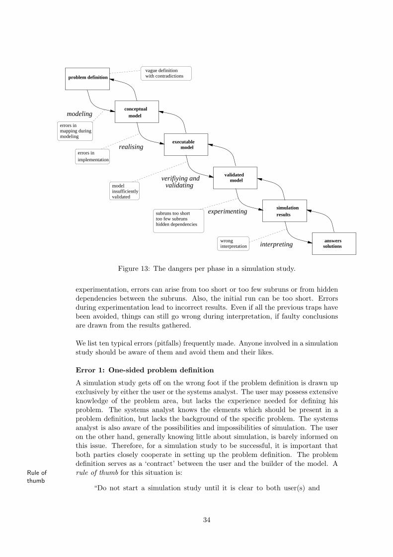
problem definition

conceptualmodel

executablemodel

answerssolutions

resultssimulation

modelvalidated

modeling

realising

verifiying andvalidating

interpreting

vague definitionwith contradictions

errors inmapping duringmodeling

errors inimplementation

modelinsufficientlyvalidated

subruns too shorttoo few subruns

interpretationwrong

hidden dependencies

experimenting

Figure 13: The dangers per phase in a simulation study.

experimentation, errors can arise from too short or too few subruns or from hiddendependencies between the subruns. Also, the initial run can be too short. Errorsduring experimentation lead to incorrect results. Even if all the previous traps havebeen avoided, things can still go wrong during interpretation, if faulty conclusionsare drawn from the results gathered.

We list ten typical errors (pitfalls) frequently made. Anyone involved in a simulationstudy should be aware of them and avoid them and their likes.

Error 1: One-sided problem definition

A simulation study gets off on the wrong foot if the problem definition is drawn upexclusively by either the user or the systems analyst. The user may possess extensiveknowledge of the problem area, but lacks the experience needed for defining hisproblem. The systems analyst knows the elements which should be present in aproblem definition, but lacks the background of the specific problem. The systemsanalyst is also aware of the possibilities and impossibilities of simulation. The useron the other hand, generally knowing little about simulation, is barely informed onthis issue. Therefore, for a simulation study to be successful, it is important thatboth parties closely cooperate in setting up the problem definition. The problemdefinition serves as a ‘contract’ between the user and the builder of the model. Arule of thumb for this situation is:Rule of

thumb“Do not start a simulation study until it is clear to both user(s) and

34

analyst(s) which questions need to be answered!”

Error 2: Choice of a wrong level of detail

In making a simulation model, one chooses a certain level of detail. In a simulationmodel for a manufacturing department, a machine may be modeled as an objectwith serving time as its only parameter. Alternatively, it can be modeled in detail,taking into account aspects such as set-up times, faults, tool-loading, maintenanceintervals etc. Many simulation studies fail because a wrong level of detail was choseninitially. Too much detail causes the model to become unnecessarily complex andintroduces extra parameters that need to be assessed (with all the risks involved).A lack of adequate detail can lead to a simulation model that leaves the essentialquestions of the problem definition unanswered. The right level of detail is chosenif:

Characteristicsof a goodlevel ofdetail

(1) information is present that allows experiments with the model,

(2) the important questions from the problem definition are addressed by themodel and

(3) the complexity of the model is still manageable for all parties concerned.

If it is impossible to choose a level of detail that meets this condition, the problemdefinition will have to be adjusted.

Error 3: Hidden assumptions

Many assumptions are needed in order to allow a simulation study to be carried out.These assumptions fill gaps in an incomplete problem definition or are made to keepthe simulation model simple. The assumptions should be carefully documentedand reported, as provisos for the conclusions. If possible, a sensitivity analysisshould be carried out to assess how dependent the reported conclusions are of them.Assumptions that are made without proper documentation (i.e. hidden) have thetendency to evolve into unquestioned truths. Incorrect hidden assumptions maylead to the rejection of the simulation model. Also, hidden assumptions aboutfuture developments lead to incorrect conclusions. There is quite some differencebetween the conclusions The capacity will be insufficient within three years with andwithout the proviso in case of 8% annual growth.

Error 4: Validation by the wrong people

Sometimes, due to time pressure or indifference of the user, the simulation modelis only validated by its maker(s). Discrepancies between the model and the ideasof the user may thus be discovered too late, if at all. Therefore, the user shouldbe involved in the validation of the simulation model before any experiments areconducted.

Error 5: Forcing the model to fit

Frequently, in the validation phase, the results of the simulation model do not matchthe observed or recorded actual data. One is then tempted to make the model ‘fit’ by

35

changing certain parameter values. One fiddles around with the parameter settingsuntil some match is found. This, however, is very dangerous, since this match withreality is most likely caused by sheer luck and not by a model that adequately reflectsreality. Parameters should be adjusted only after having understood why the modeldeviates from reality. This prevents the conscious or unconscious obscuring of errorsin the model.

Error 6: Underexposure of the sensitivity of the model

Certain model parameters (e.g. the intensity of the arrival process) are often set atone specific value. This chosen setting should be justified statistically. However, evenif this is the case, small variations in the arrival process can make all assumptionsabout it invalid. Therefore, the sensitivity of the model to minor adjustments of theparameters should be seriously accounted for.

Error 7: No subruns

Some people say: “A sufficiently long simulation yields correct results!” They exe-cute a simulation run for a night or weekend and then blindly trust e.g. the meanwaiting time measured. This is a very risky practice, as it disallows any assertionsabout the reliability of the result found. The reported half width should be used todefine reliability intervals. In a what-if analysis through simulation, the simulationshould be carried out long enough to allow reliable comparison of alternatives.

Error 8: Careless presentation of the results

Interpreting the results of a simulation study may require complex statistical analy-sis. This is often a source of errors. Translating the results from statistics intolanguage a user can understand, can be very tricky indeed. In Darrel Huff’s book“How to lie with statistics” ([4]), there are numerous examples of sloppy and mis-leading presentations. As an example, suppose the final report of a simulation studycontains the following conclusion “Waiting times will be reduced by 10 percent”.This conclusion is very incomplete, as it contains no reference whatsoever to itsreliability. It is good practice to give a confidence interval. The same conclusionsuggests that waiting times will be reduced by 10 percent for each customer. This,however, may not be the case. The average waiting time may be reduced by 10percent while it increases for certain customers and is reduced somewhat more forothers.

Error 9: Dangers of animation

Simulation tools present nicely formatted reports and even possess animation facili-ties. This improves communication with the user. However, there is a large inherentdanger in animation. As animation only shows the tangible aspects of the simula-tion model, the user may develop an unfounded faith in the model. The choice ofparameters or decision making rules deeply influence the simulation results, yet arebarely visible in an animation. A nice report does not replace a sound statisticalanalysis.

36

Error 10: Unnecessary use of simulation

Simulation is a flexible and varied analysis tool. Some people therefore are inclinedto use it regardless of the circumstances. Often, however, a simple mathematicalmodel (e.g. a queuing model) or a simple spreadsheet calculation is sufficient. Insuch cases simulation is ‘overkill’. It should only be used if and when the situationrequires it. Simulation is a means and not a goal!

8 Recommended further reading

A classic book on simulation is the book by Naylor et al. [9]. Other standardworks about simulation are: Bratley, Fox and Schrage [2], Law and Kelton [7], Ross[11] and Shannon [12]. In particular the books of Ross ([11]) and Bratley, Fox andSchrage ([2]) are recommended for further study.

37

References

[1] F. Baskett, K.M. Chandy, R.R. Muntz, and F.G. Palacios. Open, Closed andMixed Networks of Queues with Different Classes of Customers. Journal of theAssociation of Computing Machinery, 22(2):248–260, April 1975.

[2] P. Bratley, B.L. Fox, and L.E. Schrage. A guide to simulation, 2nd ed. Springer-Verlag, Berlin, 1987.

[3] D. Gross and C.M. Harris. Fundamentals of queueing theory. Wiley, London,1985.

[4] D. Huff. How to lie with statistics. Penguin Books, New York, 1954.

[5] W.D. Kelton, R.P. Sadowski, and D. Sturrock. Simulation with Arena, 3rd ed.McGraw-Hill, New York, 2004.

[6] L. Kleinrock. Queueing systems, Vol. 1:Theory. Wiley-Interscience, London,1975.

[7] A.M. Law and W.D. Kelton. Simulation modeling and analysis, 3rd ed.McGraw-Hill, New York, 2000.

[8] M. Ajmone Marsan, G. Balbo, and G. Conte. Performance Models of Multi-processor Systems. The MIT Press, Cambridge, 1986.

[9] T.H. Naylor, J.L. Balintfy, D.S. Burdick, and Kong Chu. Computer simulationtechniques. Wiley, New York, 1966.

[10] M. Pidd. Computer modelling for discrete simulation, 4th ed. Wiley, Chichester,2002.

[11] S.M. Ross. A course in simulation, 3rd edition. Academic Press, San Diego,2002.

[12] R.E. Shannon. Systems simulation: the art and science. Prentice-Hall, Engle-wood Cliffs, 1975.

38

A Modeling, concurrency and scheduling with Petri nets

In this appendix we treat the concurrency aspect of simulation: actions may ormay not occur simultaneously. This influences the order in which the actions arescheduled and their interaction with the simulated time. These concepts are vitalto simulation models; they are best illustrated within Petri nets but are not limitedto them alone.Petri net modeling is all about the interplay of actions and objects. Actions may ormay not occur depending upon the presence of certain objects. Of course, it is nearimpossible to take all kinds of objects into account. Whether or not a certain objectmust be modeled depends on the questions that need an answer. The same holdsfor actions.We revisit our discotheque example. We are interested in the cloakroom queues. sothe actions that we wish to model are entering, leaving one’s coat and departing.There are possible queues for leaving and obtaining one’s coat. A first approximationfeatures customer objects as shown in Figure 14. A customer can be in five states:outside (wishing to enter), in the hall (queuing to leave his/her coat), inside, inthe hall (queuing to get his/her coat) and outside (having left). These states arevisible as circles and are called places. The actions are inscribed in squares calledtransitions. They move the customers from one state to the other. We add atransition that moves customers from in to qgc.

in

lc gcwlent

out1 out2qlc qgc

Figure 14: Discotheque simulation model.

In the figure, the customer objects are visible as tokens, the black dots within theplaces. From time to time, a customer moves from one state to another. This isunderstood as the consumption of a token and the production of a new token. Inthe depicted model, there are three customers waiting to leave their coat and onewaiting to get it.In Figure 14, a customer could move from place qlc ot place in. In order to determinethe time at which such a state change occurs, every token possesses a time stamp.By looking at the time stamps of the tokens, a scheduler of the simulation decidesScheduler

the next action that will occur and the simulated occurrence time of that action.A logical rule for the scheduler is that an action cannot occur sooner than the timestamps of the tokens consumed by it. Another rule is called the eagerness rule: ifEagerness

some action can occur, some action must occur. If an action occurs, the time stampsof the produced tokens will be greater than or equal to the simulated time of thataction. Often, a delay depending on the action is added to the occurrence time.We shall study the example in Figure 15. Initially there are three tokens with timestamps 5,6, and 6 in place a. Action x has a delay of 2 and y has a delay of 0.Action x can occur at time 5, so by the eagerness rule some action must occur attime 5. The only action that can occur is x, consuming the token with time stamp5 and producing a token with time stamp 7 because of the delay. So we obtain thesecond token configuration. In this configuration, there are two possibilities for x

39

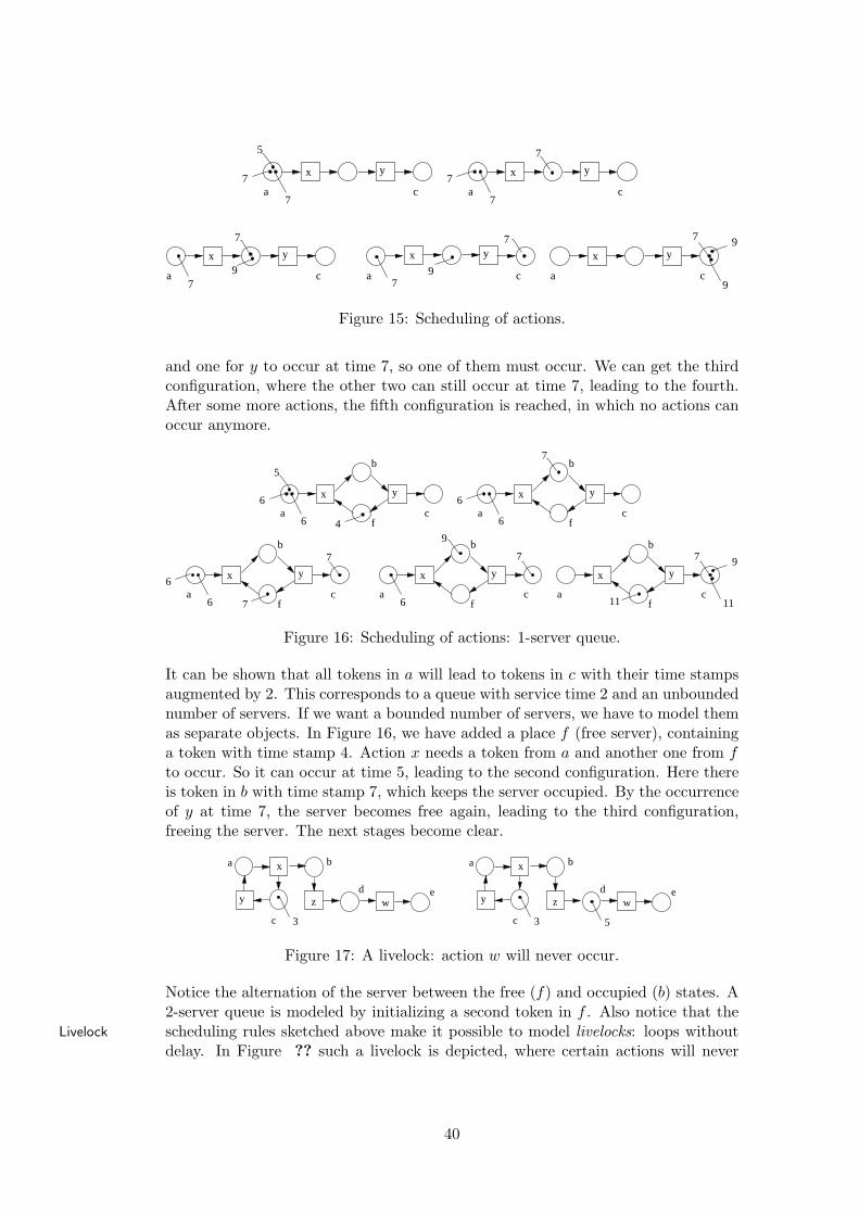
x y x y

x y x y x y

a c

5

7

7

a c7

a c7

7

a c a c

7 9

9

7

7

97

9

7

Figure 15: Scheduling of actions.

and one for y to occur at time 7, so one of them must occur. We can get the thirdconfiguration, where the other two can still occur at time 7, leading to the fourth.After some more actions, the fifth configuration is reached, in which no actions canoccur anymore.

a c

x y

5

6

6

b

f

a c

x y6

6

b

f

a c

x y6

6

b

f

a c

x y

6

b

fa c

x y

b

f

7

4

7

7

9

7 7 9

1111

Figure 16: Scheduling of actions: 1-server queue.

It can be shown that all tokens in a will lead to tokens in c with their time stampsaugmented by 2. This corresponds to a queue with service time 2 and an unboundednumber of servers. If we want a bounded number of servers, we have to model themas separate objects. In Figure 16, we have added a place f (free server), containinga token with time stamp 4. Action x needs a token from a and another one from fto occur. So it can occur at time 5, leading to the second configuration. Here thereis token in b with time stamp 7, which keeps the server occupied. By the occurrenceof y at time 7, the server becomes free again, leading to the third configuration,freeing the server. The next stages become clear.

c

y

3

a b

d e

x

z w

c

y

3

a b

d e

x

z w

5

Figure 17: A livelock: action w will never occur.

Notice the alternation of the server between the free (f) and occupied (b) states. A2-server queue is modeled by initializing a second token in f . Also notice that thescheduling rules sketched above make it possible to model livelocks: loops withoutLivelock

delay. In Figure ?? such a livelock is depicted, where certain actions will never

40

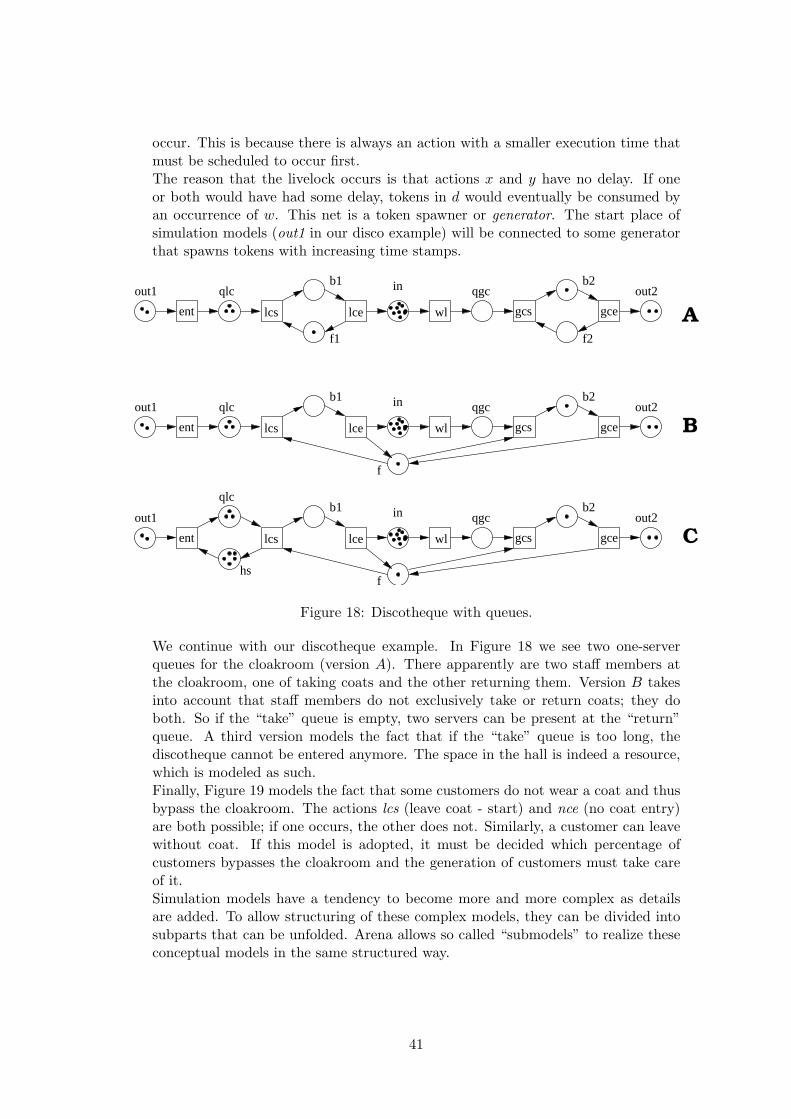
occur. This is because there is always an action with a smaller execution time thatmust be scheduled to occur first.The reason that the livelock occurs is that actions x and y have no delay. If oneor both would have had some delay, tokens in d would eventually be consumed byan occurrence of w. This net is a token spawner or generator. The start place ofsimulation models (out1 in our disco example) will be connected to some generatorthat spawns tokens with increasing time stamps.

qlc

ent

in

lcs lce

out1 qlc

f1

b1

ent

in

lcs lce

out1 qlcb1

ent

in

lcs lce

out1b1

out2

gcs gce

b2

out2

gcs gce

b2

out2

gcs gce

b2

A

B

C

qgc

qgc

qgc

f2

f

f

wl

wl

wl

hs

Figure 18: Discotheque with queues.

We continue with our discotheque example. In Figure 18 we see two one-serverqueues for the cloakroom (version A). There apparently are two staff members atthe cloakroom, one of taking coats and the other returning them. Version B takesinto account that staff members do not exclusively take or return coats; they doboth. So if the “take” queue is empty, two servers can be present at the “return”queue. A third version models the fact that if the “take” queue is too long, thediscotheque cannot be entered anymore. The space in the hall is indeed a resource,which is modeled as such.Finally, Figure 19 models the fact that some customers do not wear a coat and thusbypass the cloakroom. The actions lcs (leave coat - start) and nce (no coat entry)are both possible; if one occurs, the other does not. Similarly, a customer can leavewithout coat. If this model is adopted, it must be decided which percentage ofcustomers bypasses the cloakroom and the generation of customers must take careof it.Simulation models have a tendency to become more and more complex as detailsare added. To allow structuring of these complex models, they can be divided intosubparts that can be unfolded. Arena allows so called “submodels” to realize theseconceptual models in the same structured way.

41

������������������������������������������������������������������������������������

������������������������������������������������������������������������������������

������������������������������������������������������������������������

������������������������������������������������������������������������

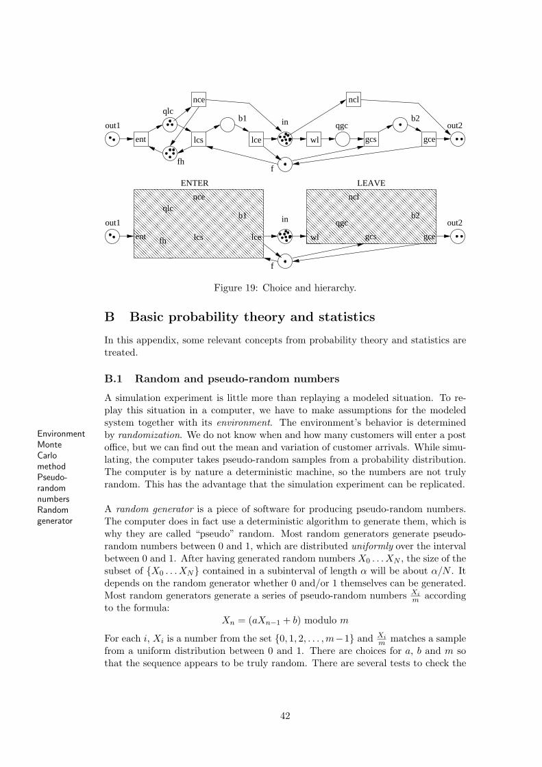
ent

in

lcs lce

out1b1

out2

gcs gce

b2qgc

f

wl

qlcnce ncl

fh

in out2

gcs gce

b2qgc

f

wl

ncl

out1

ent lcs lce

b1qlc

nce

fh

LEAVEENTER

Figure 19: Choice and hierarchy.

B Basic probability theory and statistics

In this appendix, some relevant concepts from probability theory and statistics aretreated.

B.1 Random and pseudo-random numbers

A simulation experiment is little more than replaying a modeled situation. To re-play this situation in a computer, we have to make assumptions for the modeledsystem together with its environment. The environment’s behavior is determined

Environment by randomization. We do not know when and how many customers will enter a postMonteCarlomethod

office, but we can find out the mean and variation of customer arrivals. While simu-lating, the computer takes pseudo-random samples from a probability distribution.

Pseudo-randomnumbers

The computer is by nature a deterministic machine, so the numbers are not trulyrandom. This has the advantage that the simulation experiment can be replicated.

A random generator is a piece of software for producing pseudo-random numbers.Randomgenerator The computer does in fact use a deterministic algorithm to generate them, which is

why they are called “pseudo” random. Most random generators generate pseudo-random numbers between 0 and 1, which are distributed uniformly over the intervalbetween 0 and 1. After having generated random numbers X0 . . . XN , the size of thesubset of {X0 . . . XN} contained in a subinterval of length α will be about α/N . Itdepends on the random generator whether 0 and/or 1 themselves can be generated.Most random generators generate a series of pseudo-random numbers Xi

m accordingto the formula:

Xn = (aXn−1 + b) modulo m

For each i, Xi is a number from the set {0, 1, 2, . . . , m−1} and Xim matches a sample

from a uniform distribution between 0 and 1. There are choices for a, b and m sothat the sequence appears to be truly random. There are several tests to check the

42

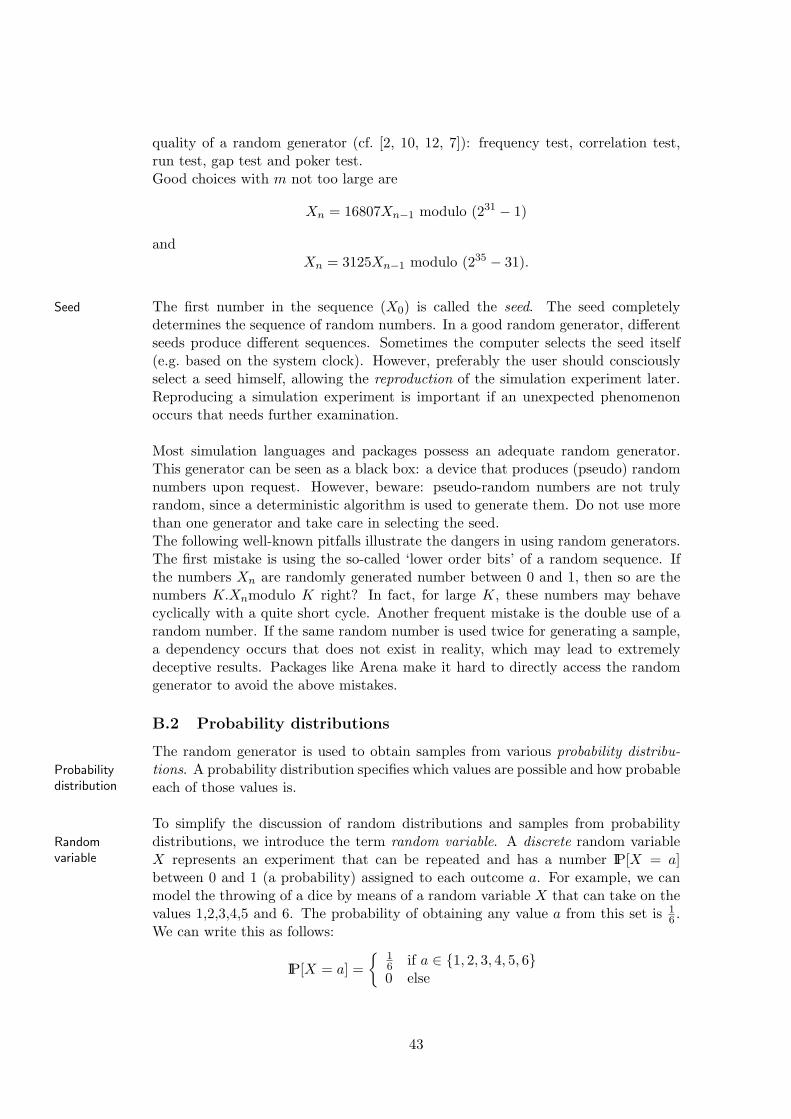
quality of a random generator (cf. [2, 10, 12, 7]): frequency test, correlation test,run test, gap test and poker test.Good choices with m not too large are

Xn = 16807Xn−1 modulo (231 − 1)

andXn = 3125Xn−1 modulo (235 − 31).

The first number in the sequence (X0) is called the seed. The seed completelySeed

determines the sequence of random numbers. In a good random generator, differentseeds produce different sequences. Sometimes the computer selects the seed itself(e.g. based on the system clock). However, preferably the user should consciouslyselect a seed himself, allowing the reproduction of the simulation experiment later.Reproducing a simulation experiment is important if an unexpected phenomenonoccurs that needs further examination.

Most simulation languages and packages possess an adequate random generator.This generator can be seen as a black box: a device that produces (pseudo) randomnumbers upon request. However, beware: pseudo-random numbers are not trulyrandom, since a deterministic algorithm is used to generate them. Do not use morethan one generator and take care in selecting the seed.The following well-known pitfalls illustrate the dangers in using random generators.The first mistake is using the so-called ‘lower order bits’ of a random sequence. Ifthe numbers Xn are randomly generated number between 0 and 1, then so are thenumbers K.Xnmodulo K right? In fact, for large K, these numbers may behavecyclically with a quite short cycle. Another frequent mistake is the double use of arandom number. If the same random number is used twice for generating a sample,a dependency occurs that does not exist in reality, which may lead to extremelydeceptive results. Packages like Arena make it hard to directly access the randomgenerator to avoid the above mistakes.

B.2 Probability distributions

The random generator is used to obtain samples from various probability distribu-tions. A probability distribution specifies which values are possible and how probableProbability

distribution each of those values is.

To simplify the discussion of random distributions and samples from probabilitydistributions, we introduce the term random variable. A discrete random variableRandom

variable X represents an experiment that can be repeated and has a number IP[X = a]between 0 and 1 (a probability) assigned to each outcome a. For example, we canmodel the throwing of a dice by means of a random variable X that can take on thevalues 1,2,3,4,5 and 6. The probability of obtaining any value a from this set is 1

6 .We can write this as follows:

IP[X = a] ={

16 if a ∈ {1, 2, 3, 4, 5, 6}0 else

43

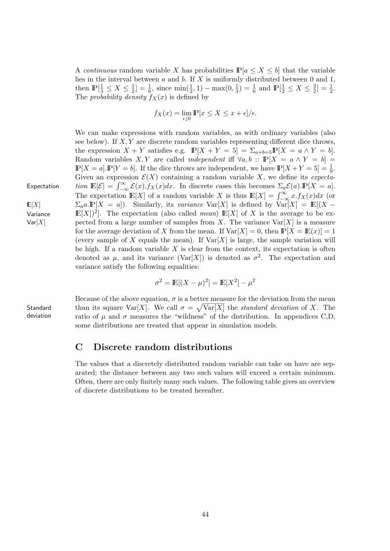
A continuous random variable X has probabilities IP[a ≤ X ≤ b] that the variablelies in the interval between a and b. If X is uniformly distributed between 0 and 1,then IP[13 ≤ X ≤ 1

2 ] = 16 , since min(1

2 , 1) −max(0, 13) = 1

6 and IP[12 ≤ X ≤ 32 ] = 1

2 .The probability density fX(x) is defined by

fX(x) = limε↓0

IP[x ≤ X ≤ x + ε]/ε.

We can make expressions with random variables, as with ordinary variables (alsosee below). If X,Y are discrete random variables representing different dice throws,the expression X + Y satisfies e.g. IP[X + Y = 5] = Σa+b=5IP[X = a ∧ Y = b].Random variables X, Y are called independent iff ∀a, b :: IP[X = a ∧ Y = b] =IP[X = a].IP[Y = b]. If the dice throws are independent, we have IP[X +Y = 5] = 1

9 .Given an expression E(X) containing a random variable X, we define its expecta-tion IE[E ] =

∫∞−∞ E(x).fX(x)dx. In discrete cases this becomes ΣaE(a).IP[X = a].Expectation

The expectation IE[X] of a random variable X is thus IE[X] =∫∞−∞ x.fX(x)dx (or

Σaa.IP[X = a]). Similarly, its variance Var[X] is defined by Var[X] = IE[(X −IE[X]Variance IE[X])2]. The expectation (also called mean) IE[X] of X is the average to be ex-Var[X] pected from a large number of samples from X. The variance Var[X] is a measure

for the average deviation of X from the mean. If Var[X] = 0, then IP[X = IE(x)] = 1(every sample of X equals the mean). If Var[X] is large, the sample variation willbe high. If a random variable X is clear from the context, its expectation is oftendenoted as µ, and its variance (Var[X]) is denoted as σ2. The expectation andvariance satisfy the following equalities:

σ2 = IE[(X − µ)2] = IE[X2]− µ2

Because of the above equation, σ is a better measure for the deviation from the meanthan its square Var[X]. We call σ =

√Var[X] the standard deviation of X. TheStandard

deviation ratio of µ and σ measures the “wildness” of the distribution. In appendices C,D,some distributions are treated that appear in simulation models.

C Discrete random distributions

The values that a discretely distributed random variable can take on have are sep-arated; the distance between any two such values will exceed a certain minimum.Often, there are only finitely many such values. The following table gives an overviewof discrete distributions to be treated hereafter.

44

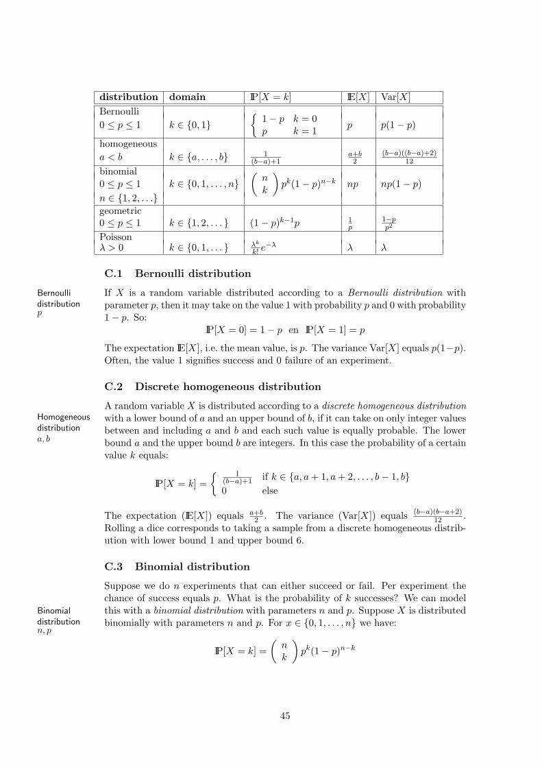
distribution domain IP[X = k] IE[X] Var[X]Bernoulli0 ≤ p ≤ 1 k ∈ {0, 1}

{1− p k = 0p k = 1

p p(1− p)

homogeneousa < b k ∈ {a, . . . , b} 1

(b−a)+1a+b2

(b−a)((b−a)+2)12

binomial0 ≤ p ≤ 1 k ∈ {0, 1, . . . , n}

(nk

)pk(1− p)n−k np np(1− p)

n ∈ {1, 2, . . .}geometric0 ≤ p ≤ 1 k ∈ {1, 2, . . . } (1− p)k−1p 1

p1−pp2

Poissonλ > 0 k ∈ {0, 1, . . . } λk

k! e−λ λ λ

C.1 Bernoulli distribution

If X is a random variable distributed according to a Bernoulli distribution withBernoullidistribution parameter p, then it may take on the value 1 with probability p and 0 with probabilityp 1− p. So:

IP[X = 0] = 1− p en IP[X = 1] = p

The expectation IE[X], i.e. the mean value, is p. The variance Var[X] equals p(1−p).Often, the value 1 signifies success and 0 failure of an experiment.

C.2 Discrete homogeneous distribution

A random variable X is distributed according to a discrete homogeneous distributionHomogeneousdistribution

with a lower bound of a and an upper bound of b, if it can take on only integer values

a, bbetween and including a and b and each such value is equally probable. The lowerbound a and the upper bound b are integers. In this case the probability of a certainvalue k equals:

IP[X = k] ={ 1

(b−a)+1 if k ∈ {a, a + 1, a + 2, . . . , b− 1, b}0 else

The expectation (IE[X]) equals a+b2 . The variance (Var[X]) equals (b−a)(b−a+2)

12 .Rolling a dice corresponds to taking a sample from a discrete homogeneous distrib-ution with lower bound 1 and upper bound 6.

C.3 Binomial distribution

Suppose we do n experiments that can either succeed or fail. Per experiment thechance of success equals p. What is the probability of k successes? We can modelthis with a binomial distribution with parameters n and p. Suppose X is distributedBinomial

distributionn, p

binomially with parameters n and p. For x ∈ {0, 1, . . . , n} we have:

IP[X = k] =(

nk

)pk(1− p)n−k

45

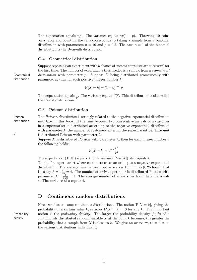
The expectation equals np. The variance equals np(1 − p). Throwing 10 coinson a table and counting the tails corresponds to taking a sample from a binomialdistribution with parameters n = 10 and p = 0.5. The case n = 1 of the binomialdistribution is the Bernoulli distribution.

C.4 Geometrical distribution

Suppose repeating an experiment with a chance of success p until we are successful forthe first time. The number of experiments thus needed is a sample from a geometricaldistribution with parameter p. Suppose X being distributed geometrically withGeometrical

distribution parameter p, then for each positive integer number k:

IP[X = k] = (1− p)k−1p

The expectation equals 1p . The variance equals 1−p

p2 . This distribution is also calledthe Pascal distribution.

C.5 Poisson distribution

The Poisson distribution is strongly related to the negative exponential distributionPoissondistribution seen later in this book. If the time between two consecutive arrivals of a customer

in a supermarket is distributed according to the negative exponential distributionwith parameter λ, the number of customers entering the supermarket per time unitis distributed Poisson with parameter λ.λ

Suppose X is distributed Poisson with parameter λ, then for each integer number kthe following holds:

IP[X = k] = e−λ λk

k!The expectation (IE[X]) equals λ. The variance (Var[X]) also equals λ.Think of a supermarket where customers enter according to a negative exponentialdistribution. The average time between two arrivals is 15 minutes (0.25 hour), thatis to say λ = 1

0.25 = 4. The number of arrivals per hour is distributed Poisson withparameter λ = 1

0.25 = 4. The average number of arrivals per hour therefore equals4. The variance also equals 4.

D Continuous random distributions

Next, we discuss some continuous distributions. The notion IP[X = k], giving theprobability of a certain value k, satisfies IP[X = k] = 0 for any k. The importantnotion is the probability density. The larger the probability density fX(k) of aProbability

density continuously distributed random variable X at the point k becomes, the greater theprobability that a sample from X is close to k. We give an overview, then discussthe various distributions individually.

46

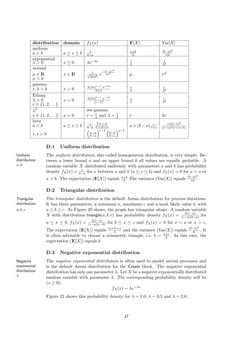
distribution domain fX(x) IE[X] Var[X]uniforma < b a ≤ x ≤ b 1

b−aa+b2

(b−a)2

12

exponentialλ > 0 x ≥ 0 λe−λx 1

λ1λ2

normalµ ∈ IR x ∈ IR 1√

2πσ2e−(x−µ)2

2σ2 µ σ2

σ > 0gammar, λ > 0 x > 0 λ(λx)r−1 e−λx

Γ(r)rλ

rλ2

Erlangλ > 0 x > 0 λ(λx)r−1 e−λx

(r−1)!rλ

rλ2

r ∈ {1, 2, . . .}χ2 see gammav ∈ {1, 2, . . .} x > 0 r = v

2 and λ = 12 v 2v

betaa < b a ≤ x ≤ b 1

b−aΓ(r+s)Γ(r)Γ(s) a + (b− a) r

r+srs(b−a)2

(r+s)2(r+s+1)

r, s > 0(

x−ab−a

)r−1 (b−xb−a

)s−1

D.1 Uniform distribution

The uniform distribution, also called homogeneous distribution, is very simple. Be-Uniformdistribution tween a lower bound a and an upper bound b all values are equally probable. Aa, b random variable X distributed uniformly with parameters a and b has probability

density fX(x) = 1b−a for x between a and b (a ≤ x ≤ b) and fX(x) = 0 for x < a or

x > b. The expectation (IE[X]) equals a+b2 The variance (Var[X]) equals (b−a)2

12 .

D.2 Triangular distribution

The triangular distribution is the default Arena distribution for process durations.Triangulardistribution It has three parameters, a minimum a, maximum c and a most likely value b, with

a ≤ b ≤ c. As Figure 20 shows, the graph has triangular shape. A random variablea, b, c

X with distribution triangle(a, b, c) has probability density fX(x) = 2(x−a)(c−a)(b−a) for

a ≤ x ≤ b, fX(x) = 2(c−x)(c−a)(c−b) for b ≤ x ≤ c and fX(x) = 0 for x < a or x > c.

The expectation (IE[X]) equals (a+b+c)3 and the variance (Var[X]) equals (b−a)2

6 . Itis often advisable to choose a symmetric triangle, i.e. b = a+c

2 . In this case, theexpectation (IE[X]) equals b.

D.3 Negative exponential distribution

The negative exponential distribution is often used to model arrival processes andNegativeexponentialdistribution

is the default Arena distribution for the Create block. The negative exponentialdistribution has only one parameter λ. Let X be a negative exponentially distributed

λ random variable with parameter λ. The corresponding probability density will be(x ≥ 0):

fX(x) = λe−λx

Figure 21 shows this probability density for λ = 1.0, λ = 0.5 and λ = 2.0.

47

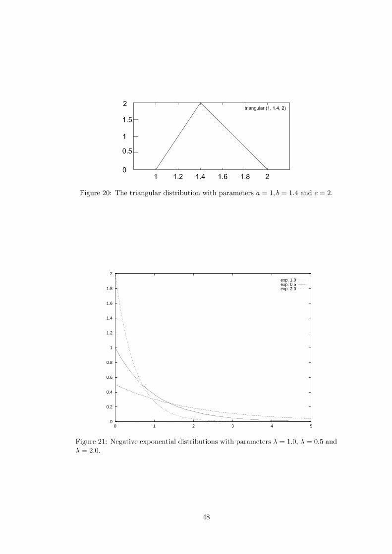
triangular (1, 1.4, 2)

Figure 20: The triangular distribution with parameters a = 1, b = 1.4 and c = 2.

0

0.2

0.4

0.6

0.8

1

1.2

1.4

1.6

1.8

2

0 1 2 3 4 5

exp. 1.0exp. 0.5exp. 2.0

Figure 21: Negative exponential distributions with parameters λ = 1.0, λ = 0.5 andλ = 2.0.

48

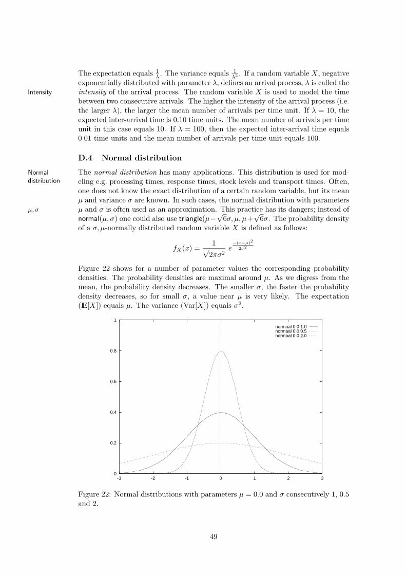
The expectation equals 1λ . The variance equals 1

λ2 . If a random variable X, negativeexponentially distributed with parameter λ, defines an arrival process, λ is called theintensity of the arrival process. The random variable X is used to model the timeIntensity

between two consecutive arrivals. The higher the intensity of the arrival process (i.e.the larger λ), the larger the mean number of arrivals per time unit. If λ = 10, theexpected inter-arrival time is 0.10 time units. The mean number of arrivals per timeunit in this case equals 10. If λ = 100, then the expected inter-arrival time equals0.01 time units and the mean number of arrivals per time unit equals 100.

D.4 Normal distribution

The normal distribution has many applications. This distribution is used for mod-Normaldistribution eling e.g. processing times, response times, stock levels and transport times. Often,

one does not know the exact distribution of a certain random variable, but its meanµ and variance σ are known. In such cases, the normal distribution with parametersµ and σ is often used as an approximation. This practice has its dangers; instead ofµ, σ

normal(µ, σ) one could also use triangle(µ−√6σ, µ, µ+√

6σ. The probability densityof a σ, µ-normally distributed random variable X is defined as follows:

fX(x) =1√

2πσ2e−(x−µ)2

2σ2

Figure 22 shows for a number of parameter values the corresponding probabilitydensities. The probability densities are maximal around µ. As we digress from themean, the probability density decreases. The smaller σ, the faster the probabilitydensity decreases, so for small σ, a value near µ is very likely. The expectation(IE[X]) equals µ. The variance (Var[X]) equals σ2.

0

0.2

0.4

0.6

0.8

1

-3 -2 -1 0 1 2 3

normaal 0.0 1.0normaal 0.0 0.5normaal 0.0 2.0

Figure 22: Normal distributions with parameters µ = 0.0 and σ consecutively 1, 0.5and 2.

49

If µ = 0 and σ = 1, we call this a standard normal distribution. If Y is a standardStandardnormaldistribution

normally distributed random variable, then X = µ + σY is a normally distributedrandom variable with parameters µ and σ. Conversely, if X is a normally distributedrandom variable with parameters µ and σ, then Y = X−µ

σ is a standard normallydistributed random variable.

If we use a normally distributed random variable for modeling time durations, likeprocessing times, response times or transport times, we must be aware that thisrandom variable can also take on negative values. In general negative durations areimpossible; this may even cause a failure of the simulation software. For wildlydistributed durations (like traveling from Eindhoven to Utrecht in a car), it is quitepossible that a sample duration (3 hours due to a traffic jam) exceeds twice themean duration of 1 hour. These durations are highly asymmetric: the minimumduration is, say, 50 minutes, 95% of the trips are in less than 1 hour and only in afew cases do long sample durations occur. In such cases, the next distribution is abetter choice.

D.5 Gamma distribution

A characteristic of the normal distribution is its symmetry. We often need ‘skewed’distributions instead, where the probability densities below and above the meanare distributed differently. In this case a gamma distribution might be chosen. AGamma

distribution random variable X is gamma distributed with parameters r > 0 and λ > 0 if for allr, λ x > 0:

fX(x) =λ(λx)r−1 e−λx

Γ(r)

(The function Γ is the mathematical gamma function.) Figures 23, 24 and 25 showthe probability densities for a number of parameter values.These figures clearly show that the gamma distribution, depending on the parametervalues has many manifestations. If r does not exceed 1, fX is a monotonouslydecreasing function. In this case values close to 0 are most probable. If r > 1,the function will first grow to a maximum and then decrease monotonously. Theparameter r therefore determines the shape of the distribution. The parameter λdetermines the ‘spread’ of the distribution. The larger λ, the more probable is avalue close to 0. The expectation (IE[X]) equals r

λ . The variance (Var[X]) equalsrλ2 .

The modal value of a probability distribution is the value for which the probabilityModal value

density is maximal, i.e. m is the modal value of an X if for each x: fX(m) ≥ fX(x).The modal value of a gamma distributed random variable X depends on r and λ.If r ≤ 1, 0 is the most probable value, i.e. the modal value of X equals 0. If r > 1the modal value equals r−1

λ . A special case of gamma distribution is the negativeexponential distribution (r = 1).

D.6 Erlang distribution

The Erlang distribution is a special case of the gamma distribution. A gammaErlangdistribution distribution with an integer parameter r, is also called an Erlang distribution. A

50

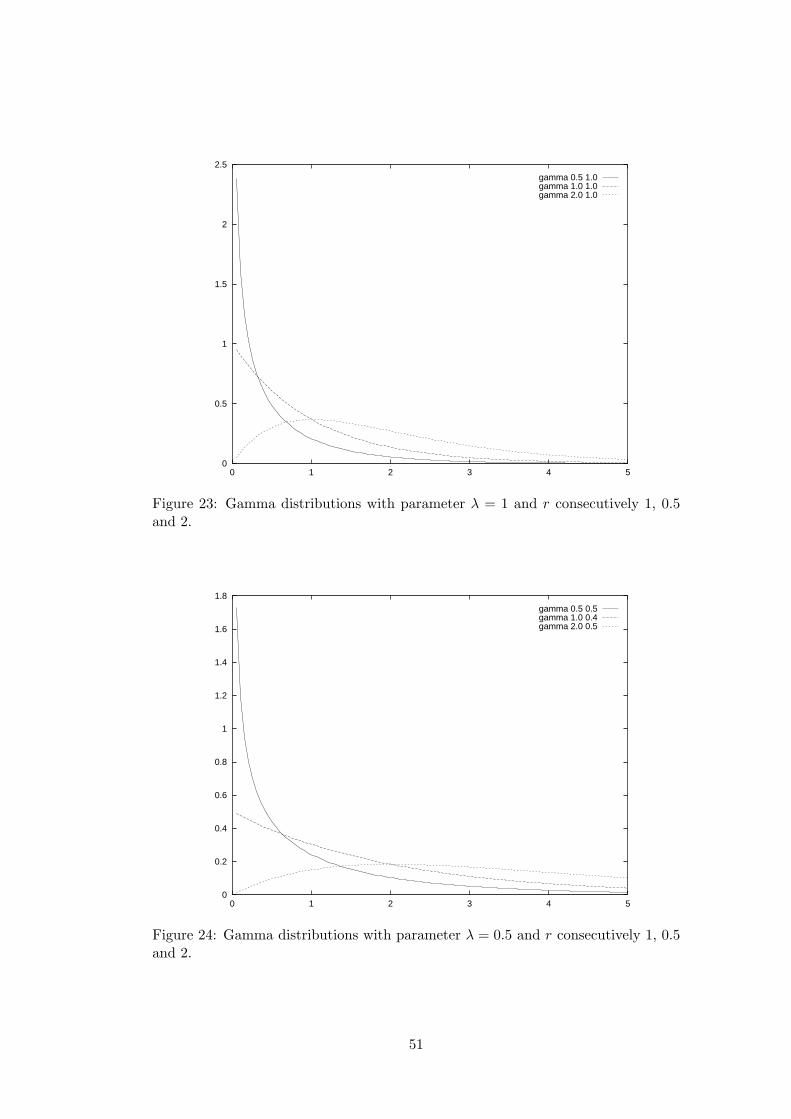
0

0.5

1

1.5

2

2.5

0 1 2 3 4 5

gamma 0.5 1.0gamma 1.0 1.0gamma 2.0 1.0

Figure 23: Gamma distributions with parameter λ = 1 and r consecutively 1, 0.5and 2.

0

0.2

0.4

0.6

0.8

1

1.2

1.4

1.6

1.8

0 1 2 3 4 5

gamma 0.5 0.5gamma 1.0 0.4gamma 2.0 0.5

Figure 24: Gamma distributions with parameter λ = 0.5 and r consecutively 1, 0.5and 2.

51

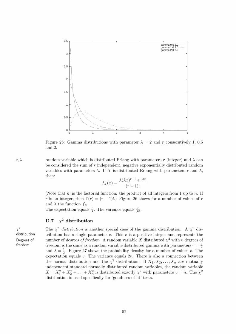
0

0.5

1

1.5

2

2.5

3

3.5

0 1 2 3 4 5

gamma 0.5 2.0gamma 1.0 2.0gamma 2.0 2.0

Figure 25: Gamma distributions with parameter λ = 2 and r consecutively 1, 0.5and 2.

random variable which is distributed Erlang with parameters r (integer) and λ canr, λ

be considered the sum of r independent, negative exponentially distributed randomvariables with parameters λ. If X is distributed Erlang with parameters r and λ,then:

fX(x) =λ(λx)r−1 e−λx

(r − 1)!

(Note that n! is the factorial function: the product of all integers from 1 up to n. Ifr is an integer, then Γ(r) = (r − 1)!.) Figure 26 shows for a number of values of rand λ the function fX .The expectation equals r

λ . The variance equals rλ2 .

D.7 χ2 distribution

The χ2 distribution is another special case of the gamma distribution. A χ2 dis-χ2

distribution tribution has a single parameter v. This v is a positive integer and represents thenumber of degrees of freedom. A random variable X distributed χ2 with v degrees ofDegrees of

freedom freedom is the same as a random variable distributed gamma with parameters r = v2

and λ = 12 . Figure 27 shows the probability density for a number of values v. The

expectation equals v. The variance equals 2v. There is also a connection betweenthe normal distribution and the χ2 distribution. If X1, X2, . . . , Xn are mutuallyindependent standard normally distributed random variables, the random variableX = X2

1 + X22 + . . . + X2

n is distributed exactly χ2 with parameters v = n. The χ2

distribution is used specifically for ‘goodness-of-fit’ tests.

52

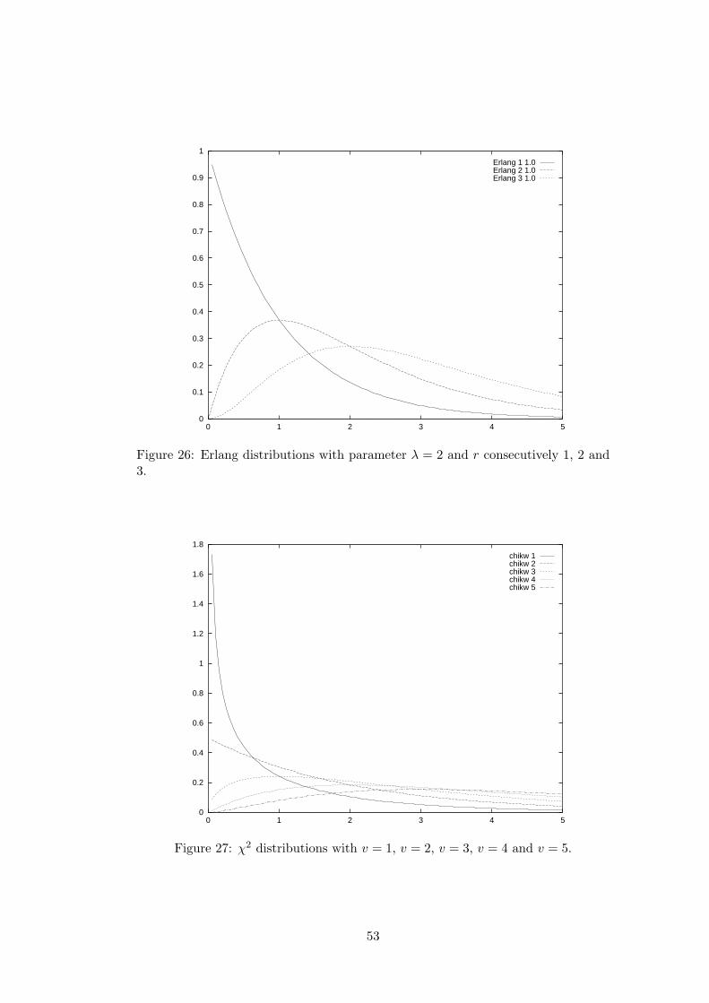
0

0.1

0.2

0.3

0.4

0.5

0.6

0.7

0.8

0.9

1

0 1 2 3 4 5

Erlang 1 1.0Erlang 2 1.0Erlang 3 1.0

Figure 26: Erlang distributions with parameter λ = 2 and r consecutively 1, 2 and3.

0

0.2

0.4

0.6

0.8

1

1.2

1.4

1.6

1.8

0 1 2 3 4 5

chikw 1chikw 2chikw 3chikw 4chikw 5

Figure 27: χ2 distributions with v = 1, v = 2, v = 3, v = 4 and v = 5.

53

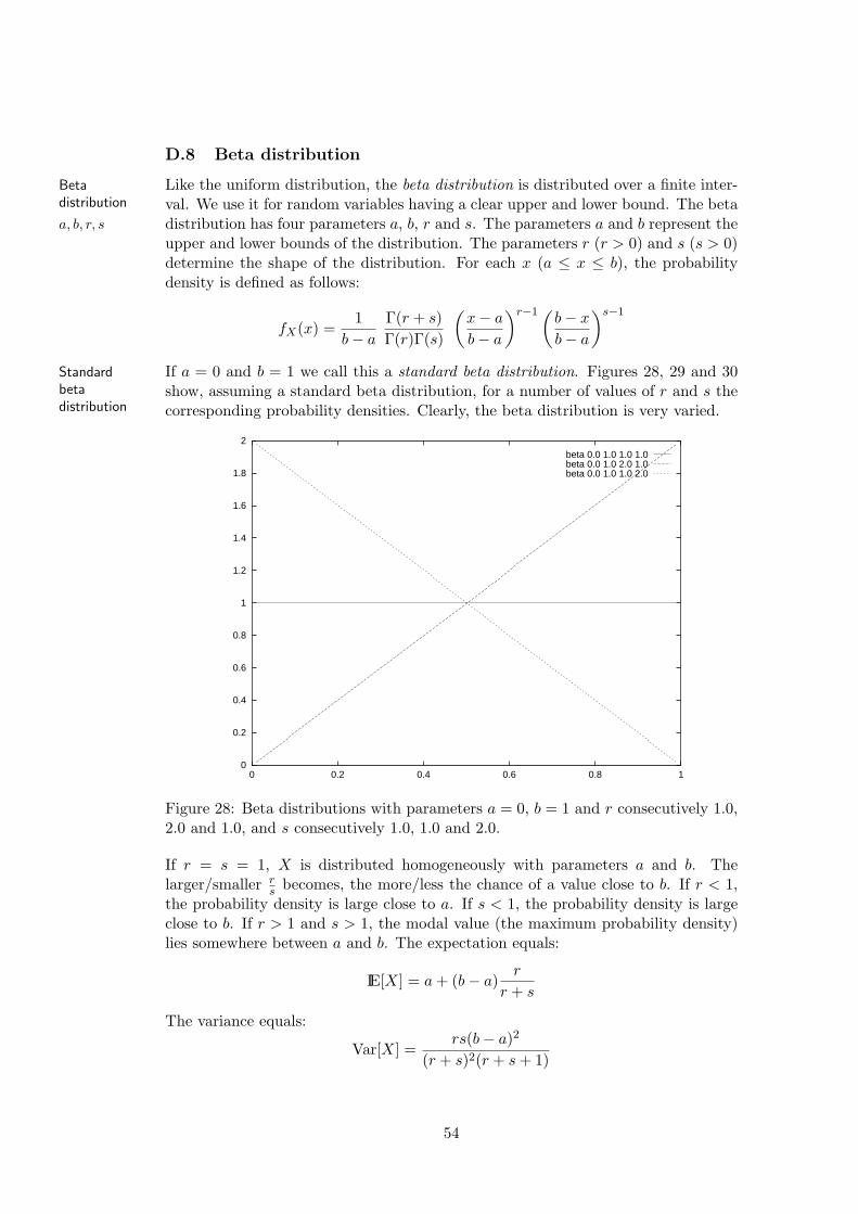
D.8 Beta distribution

Like the uniform distribution, the beta distribution is distributed over a finite inter-Betadistribution val. We use it for random variables having a clear upper and lower bound. The beta

distribution has four parameters a, b, r and s. The parameters a and b represent thea, b, r, s

upper and lower bounds of the distribution. The parameters r (r > 0) and s (s > 0)determine the shape of the distribution. For each x (a ≤ x ≤ b), the probabilitydensity is defined as follows:

fX(x) =1

b− a

Γ(r + s)Γ(r)Γ(s)

(x− a

b− a

)r−1 (b− x

b− a

)s−1

If a = 0 and b = 1 we call this a standard beta distribution. Figures 28, 29 and 30Standardbetadistribution

show, assuming a standard beta distribution, for a number of values of r and s thecorresponding probability densities. Clearly, the beta distribution is very varied.

0

0.2

0.4

0.6

0.8

1

1.2

1.4

1.6

1.8

2

0 0.2 0.4 0.6 0.8 1

beta 0.0 1.0 1.0 1.0beta 0.0 1.0 2.0 1.0beta 0.0 1.0 1.0 2.0

Figure 28: Beta distributions with parameters a = 0, b = 1 and r consecutively 1.0,2.0 and 1.0, and s consecutively 1.0, 1.0 and 2.0.

If r = s = 1, X is distributed homogeneously with parameters a and b. Thelarger/smaller r

s becomes, the more/less the chance of a value close to b. If r < 1,the probability density is large close to a. If s < 1, the probability density is largeclose to b. If r > 1 and s > 1, the modal value (the maximum probability density)lies somewhere between a and b. The expectation equals:

IE[X] = a + (b− a)r

r + s

The variance equals:

Var[X] =rs(b− a)2

(r + s)2(r + s + 1)

54

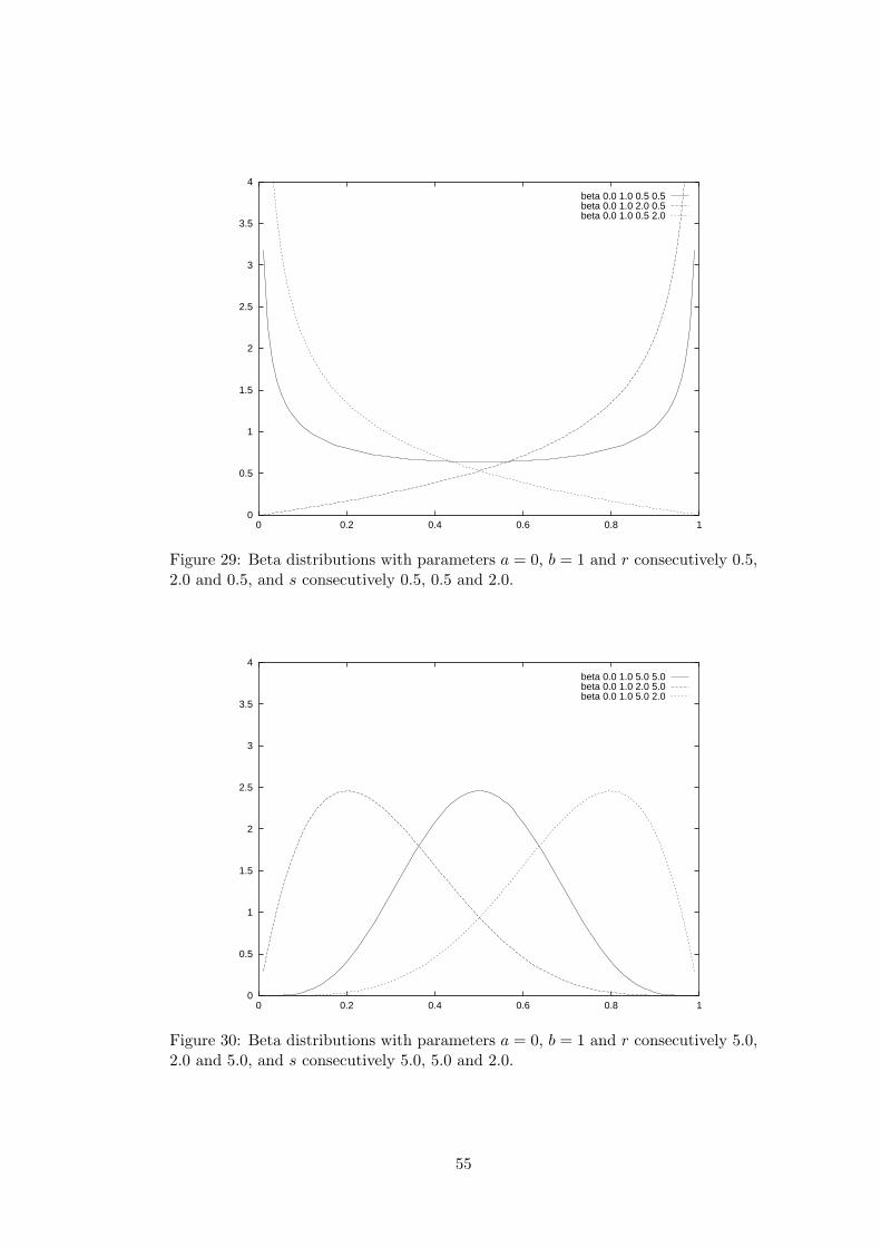
0

0.5

1

1.5

2

2.5

3

3.5

4

0 0.2 0.4 0.6 0.8 1

beta 0.0 1.0 0.5 0.5beta 0.0 1.0 2.0 0.5beta 0.0 1.0 0.5 2.0

Figure 29: Beta distributions with parameters a = 0, b = 1 and r consecutively 0.5,2.0 and 0.5, and s consecutively 0.5, 0.5 and 2.0.

0

0.5

1

1.5

2

2.5

3

3.5

4

0 0.2 0.4 0.6 0.8 1

beta 0.0 1.0 5.0 5.0beta 0.0 1.0 2.0 5.0beta 0.0 1.0 5.0 2.0

Figure 30: Beta distributions with parameters a = 0, b = 1 and r consecutively 5.0,2.0 and 5.0, and s consecutively 5.0, 5.0 and 2.0.

55

A beta distribution is ‘skewed’ (not symmetrical) whenever r 6= s. Therefore, themost probable value (modal value) may differ from the expectation. If r > 1 ands > 1, the modal value equals a + (b − a) r−1

r+s−2 . If r < 1 or s < 1, the maximalprobability density is achieved at b (if r < s) or a (if s < r).Suppose we want a standard beta distribution with an expectation µ and a varianceσ2. In that case we have to choose r and s as follows:

r =µ2(1− µ)

σ2− µ

s =(1− µ)2µ

σ2− (1− µ)

This is only possible if the following condition is met:

σ2 < µ(1− µ)

As each sample is between 0 and 1, there is an upper bound to the variance (at most0.25).A beta distributed random variable Y with lower bound a, upper bound b, expec-tation µ and variance σ2, is obtained by constructing a random variable X, distrib-uted standard beta with expectation µ−a

b−a and variance σ2

(b−a)2. Y is then defined by

Y = (b− a)X + a.

A well-known application of the beta distribution is PERT (Program EvaluationPERT

and Review Technique). PERT is a technique used by project managers assessthroughput times. For each activity PERT needs three estimates of its duration:

(i) an optimistic estimate (i.e. a lower bound),

(ii) a pessimistic estimate (i.e. an upper bound),

(iii) an estimate of the most probable duration (modal value).

If we model the duration of such an activity by means of a beta distribution, weuse the first two estimates to determine the parameters a and b. If c is the mostprobable duration, the parameters r and s are set so that the expectation and thevariance take on the following values:

µ =a + 4c + b

6

σ2 =(b− a)2

36

Therefore, if a lower and upper bound are given, the variance is fixed.

E Random variables

In this section we treat some elementary properties of random variables. X andY are random variables with respectively expectation µX and variance σ2

X , andexpectation µY and variance σ2

Y

56

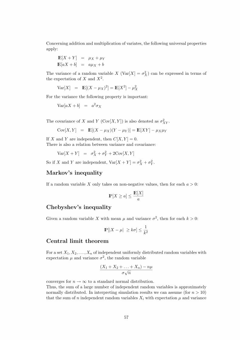
Concerning addition and multiplication of variates, the following universal propertiesapply:

IE[X + Y ] = µX + µY

IE[aX + b] = aµX + b

The variance of a random variable X (Var[X] = σ2X) can be expressed in terms of

the expectation of X and X2.

Var[X] = IE[(X − µX)2] = IE[X2]− µ2X

For the variance the following property is important:

Var[aX + b] = a2σX

The covariance of X and Y (Cov[X, Y ]) is also denoted as σ2XY .

Cov[X, Y ] = IE[(X − µX)(Y − µY )] = IE[XY ]− µXµY

If X and Y are independent, then C[X,Y ] = 0.There is also a relation between variance and covariance:

Var[X + Y ] = σ2X + σ2

Y + 2Cov[X,Y ]

So if X and Y are independent, Var[X + Y ] = σ2X + σ2

Y .

Markov’s inequality

If a random variable X only takes on non-negative values, then for each a > 0:

IP[X ≥ a] ≤ IE[X]a

Chebyshev’s inequality

Given a random variable X with mean µ and variance σ2, then for each k > 0:

IP[|X − µ| ≥ kσ] ≤ 1k2

Central limit theorem

For a set X1, X2, . . . , Xn of independent uniformly distributed random variables withexpectation µ and variance σ2, the random variable

(X1 + X2 + . . . + Xn)− nµ

σ√

n

converges for n →∞ to a standard normal distribution.Thus, the sum of a large number of independent random variables is approximatelynormally distributed. In interpreting simulation results we can assume (for n > 10)that the sum of n independent random variables Xi with expectation µ and variance

57

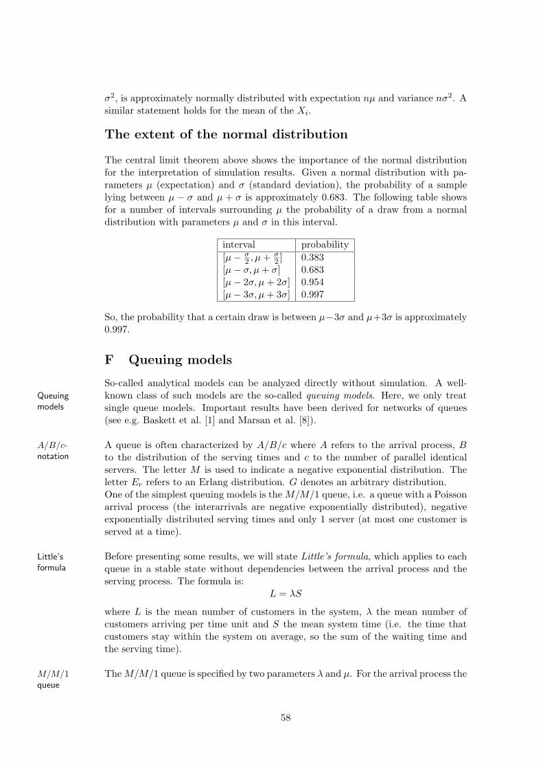
σ2, is approximately normally distributed with expectation nµ and variance nσ2. Asimilar statement holds for the mean of the Xi.

The extent of the normal distribution

The central limit theorem above shows the importance of the normal distributionfor the interpretation of simulation results. Given a normal distribution with pa-rameters µ (expectation) and σ (standard deviation), the probability of a samplelying between µ − σ and µ + σ is approximately 0.683. The following table showsfor a number of intervals surrounding µ the probability of a draw from a normaldistribution with parameters µ and σ in this interval.

interval probability[µ− σ

2 , µ + σ2 ] 0.383

[µ− σ, µ + σ] 0.683[µ− 2σ, µ + 2σ] 0.954[µ− 3σ, µ + 3σ] 0.997

So, the probability that a certain draw is between µ−3σ and µ+3σ is approximately0.997.

F Queuing models

So-called analytical models can be analyzed directly without simulation. A well-known class of such models are the so-called queuing models. Here, we only treatQueuing

models single queue models. Important results have been derived for networks of queues(see e.g. Baskett et al. [1] and Marsan et al. [8]).

A queue is often characterized by A/B/c where A refers to the arrival process, BA/B/c-notation to the distribution of the serving times and c to the number of parallel identical

servers. The letter M is used to indicate a negative exponential distribution. Theletter Er refers to an Erlang distribution. G denotes an arbitrary distribution.One of the simplest queuing models is the M/M/1 queue, i.e. a queue with a Poissonarrival process (the interarrivals are negative exponentially distributed), negativeexponentially distributed serving times and only 1 server (at most one customer isserved at a time).

Before presenting some results, we will state Little’s formula, which applies to eachLittle’sformula queue in a stable state without dependencies between the arrival process and the

serving process. The formula is:L = λS

where L is the mean number of customers in the system, λ the mean number ofcustomers arriving per time unit and S the mean system time (i.e. the time thatcustomers stay within the system on average, so the sum of the waiting time andthe serving time).

The M/M/1 queue is specified by two parameters λ and µ. For the arrival process theM/M/1queue

58

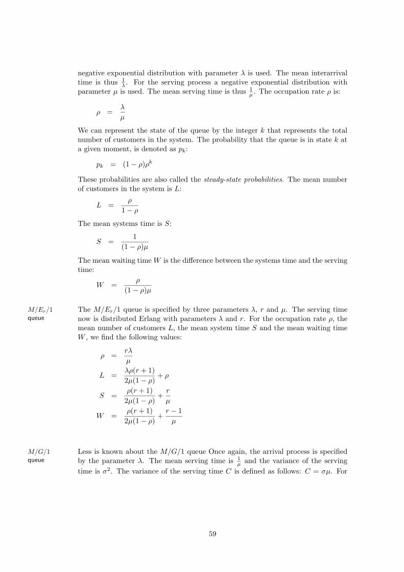
negative exponential distribution with parameter λ is used. The mean interarrivaltime is thus 1

λ . For the serving process a negative exponential distribution withparameter µ is used. The mean serving time is thus 1

µ . The occupation rate ρ is:

ρ =λ

µ

We can represent the state of the queue by the integer k that represents the totalnumber of customers in the system. The probability that the queue is in state k ata given moment, is denoted as pk:

pk = (1− ρ)ρk

These probabilities are also called the steady-state probabilities. The mean numberof customers in the system is L:

L =ρ

1− ρ

The mean systems time is S:

S =1

(1− ρ)µ

The mean waiting time W is the difference between the systems time and the servingtime:

W =ρ

(1− ρ)µ

The M/Er/1 queue is specified by three parameters λ, r and µ. The serving timeM/Er/1queue now is distributed Erlang with parameters λ and r. For the occupation rate ρ, the

mean number of customers L, the mean system time S and the mean waiting timeW , we find the following values:

ρ =rλ

µ

L =λρ(r + 1)2µ(1− ρ)

+ ρ

S =ρ(r + 1)2µ(1− ρ)

+r

µ

W =ρ(r + 1)2µ(1− ρ)

+r − 1

µ

Less is known about the M/G/1 queue Once again, the arrival process is specifiedM/G/1queue by the parameter λ. The mean serving time is 1

µ and the variance of the servingtime is σ2. The variance of the serving time C is defined as follows: C = σµ. For

59

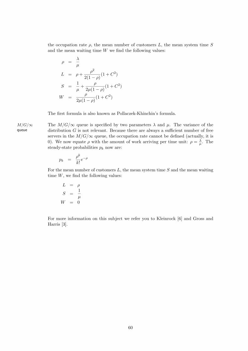
the occupation rate ρ, the mean number of customers L, the mean system time Sand the mean waiting time W we find the following values:

ρ =λ

µ

L = ρ +ρ2

2(1− ρ)(1 + C2)

S =1µ

+ρ

2µ(1− ρ)(1 + C2)

W =ρ

2µ(1− ρ)(1 + C2)

The first formula is also known as Pollaczek-Khinchin’s formula.

The M/G/∞ queue is specified by two parameters λ and µ. The variance of theM/G/∞queue distribution G is not relevant. Because there are always a sufficient number of free

servers in the M/G/∞ queue, the occupation rate cannot be defined (actually, it is0). We now equate ρ with the amount of work arriving per time unit: ρ = λ

µ . Thesteady-state probabilities pk now are:

pk =ρk

k!e−ρ

For the mean number of customers L, the mean system time S and the mean waitingtime W , we find the following values:

L = ρ

S =1µ

W = 0

For more information on this subject we refer you to Kleinrock [6] and Gross andHarris [3].

60