1

THE CHANGING NATURE OF THE BUSINESS CYCLE

RESERVE BANK OF AUSTRALIA ECONOMIC CONFERENCE

Sydney, Australia July 11-12, 2005

BUSINESS CYCLE DYNAMICS IN OECD COUNTRIES: EVIDENCE, CAUSES AND POLICY IMPLICATIONS

by Jean-Philippe Cotis and Jonathan Coppel

OECD, Economics Department1

1 Jean-Philippe Cotis is the OECD Chief Economist and Jonathan Coppel is a Senior Economist working in

Mr Cotis’s office. The authors would like to thank conference participants for their very valuable comments and questions. They also greatly benefited from Adrian Pagan’s very insightful remarks. The authors would also like to thank Debbie Bloch for her expert statistical assistance, Christophe André for programming the classical cycle dating algorithm and for useful comments and suggestions on an earlier version of this paper together with Jorgen Elmeskov, Vincent Koen and Alain de Serres. The views expressed in this paper are those of the authors and do not necessarily reflect those of the OECD Secretariat or the Organisation’s member countries.

2

Introduction

This paper deals with the interaction between economic policies and the business cycle. It focuses

more specifically on the role that improved economic policies may have played in the continuous reduction

of price and output fluctuations observed across OECD countries over the past two decades.

As suggested by the recent empirical literature, this issue remains largely unsettled. Some studies

document progress achieved over the years in the conduct of monetary policy and conclude, on an ex-ante

basis, that it must have contributed to increased price and output stability.2 Others use econometric

analysis to disentangle the respective roles played by improved monetary policies versus luck – in the form

of smaller and less frequent exogenous shocks – in explaining better outcomes.3 Overall, they do not

support the view that monetary policy had a decisive role to play in reducing price and output instability.

The present work tries to shed some additional and tentative light on these issues by examining

recent cross-country stylised facts and adopting a broader policy perspective, extending beyond monetary

policy. Focusing on the past five years, and taking a wide cross-country perspective, it suggests that the

link between ‘good’ policies and conjunctural stability could be rather strong.

More concretely, a group of countries seems to have nearly ‘extinguished’ the business cycle while

enjoying above-average trend growth. This successful group, which includes Australia, Canada, Sweden,

the United Kingdom and some others, is characterised by monetary policy frameworks of the inflation

targeting type, as well as flexible regulatory frameworks in labour, product and financial markets. These

countries are also those that undertook ambitious and comprehensive economic policy reforms over the

past couple of decades to break away from a long-standing record of weak growth trends and high price

and output instability. Therefore, it may not be pure coincidence that indicators of business cycle amplitude

for English-speaking and Nordic countries experienced a marked flattening out. 2 See Romer and Romer (2003). 3 See Stock and Watson (2004).

3

This spectacular improvement in short- and long-run performance also stands in stark contrast to

the more modest changes observed in large continental European countries, both in terms of policy reforms

and economic performance. It is indeed striking that, faced with the same sort of negative outside shocks

as continental European countries in terms of lost exports and investment, the successful group managed to

do a much better job at consumption and output smoothing over the 2001-05 period, while the stance of

fiscal and monetary policies was not particularly loose compared to the average in the large euro area

economies. In such a context, the sense of disappointment experienced in continental Europe may stem as

much from the persistence of long-standing difficulties as from the realisation that other countries have

really succeeded in improving economic performance over the years.

This combination of short-run resilience and, on average, parsimonious use of stabilisation policies

strongly suggests that structural flexibility may have been instrumental in offsetting external turbulences.

An important source of resilience seems to lie in highly flexible financial markets, in particular in the areas

of consumer and mortgage financing that have endowed monetary policy with very strong transmission

channels. The flip side of the coin may be, however, that in those resilient countries, neo-Wicksellian

monetary policies may be prone to underrating the risks for future price and output stability from out-of-

kilter asset prices.

Although this apparently outstanding performance of successful countries may be one more streak

of luck, it could also be noted that over the recent years the international environment has become

distinctly less placid. Geopolitical, oil market, as well as trade and exchange rate turbulences may have

indeed provided a more stringent and therefore convincing test of the self-stabilising propensities of

economies.

Looking at recent comparative evidence there thus seems to be a very strong prima facie case for

viewing stabilisation and structural policies as jointly determining long-term growth performance and

short-run price/output stability. Previous empirical OECD work already provided evidence that good

4

stabilisation policies brought a very significant contribution to long-term growth.4 And there is an

increasing presumption that flexible regulatory frameworks that stimulate potential growth can interact

positively with macroeconomic policies to ensure price and output stability.

Moving from descriptive statistics, comparative stylised facts and intuition to harder evidence

remains very much of a challenge, however, as well as work in progress at the OECD. Taking the

perspective of ex-ante analysis, it is relatively easy to replicate observed stylised facts and cross-country

variations through a calibrated macroeconomic maquette featuring variable degrees of price flexibility in

labour, product and financial markets as well as rule-based monetary policies (section 3.2.1). In terms of

‘ex post’ analysis, it has been possible to document, through panel data and comparative analysis, how

overly stringent regulatory frameworks are impeding price flexibility in labour, product and financial

markets and thus the reactivity of monetary policy (section 3.2.2). Finally, ex-post analysis, in the form of

SVAR modelling, is currently under way to verify that diverging output trajectories between large

continental European countries and members of the ‘successful group’ cannot be explained by differences

in shocks or macro policy stances (section 3.2.3).

These themes of interaction between economic policy and the business cycle and the role that

improved economic policy may have played in the reduction of price and output fluctuations are addressed

in the second half of this paper. In the first half, we examine the features of business cycles within

countries and the changing degree of business cycle volatility and synchronisation across countries, along

with the possible driving forces. The paper is organized as follows. The first section offers a brief overview

on the different approaches to the measurement of business cycles. The second section then examines for a

sample of 12 OECD countries some statistics and stylised facts concerning business cycles over the past 35

years, their degree of volatility and international synchronisation and how it is evolving over time. Such

statistics show indeed international convergence towards low output instability, with most spectacular

progress achieved by the English-speaking and Nordic countries. A potential trend towards increased 4 See OECD (2003a).

5

synchronisation, stricto sensu, is harder to identify. Section three analyses the latest developments in

business cycle dynamics, using recent OECD work to analyse the interaction with economic policy and

section four looks at policy implications.

1. Measuring business cycles in OECD countries

1.1 Defining the business cycle

The business cycle is usually defined as a regular and oscillatory movement in economic output

within a specified range of periodicities. How this definition is made operational has evolved over the past

half century. In the post-war period, following the seminal work of Burns and Mitchell (1946), cyclical

instability was analysed in terms of expansions and contractions in the level of economic activity, typically

measured by GDP. These cycles are known as classical business cycles.

This paper focuses only briefly on the classical cycle, because for many OECD economies declines in

the level of economic activity are rare events. There are therefore relatively few classical cycles over a 35-

year period, making it impossible to make firm inferences on how the size and length of business cycles

has evolved. An alternative and generally favoured approach to analysing the business cycle is to focus on

periods of deviations of output from trend. These episodes, which are more frequent in OECD economies,

are known as growth cycles (or deviation cycles). The analysis is concerned with phases of above and

below trend rates of growth, or movements in the output gap. Even with growth cycles, their frequency is

limited over a 35-year period, since each cycle on average lasts about 5 years.

Moving from classical to growth cycles modifies the meaning of a turning point and phase, both

concepts used to describe the morphology of a business cycle. For classical cycles, turning points are

reached when output is at a local extremum. Whereas for growth cycles, extrema are defined in terms of

output gaps.

6

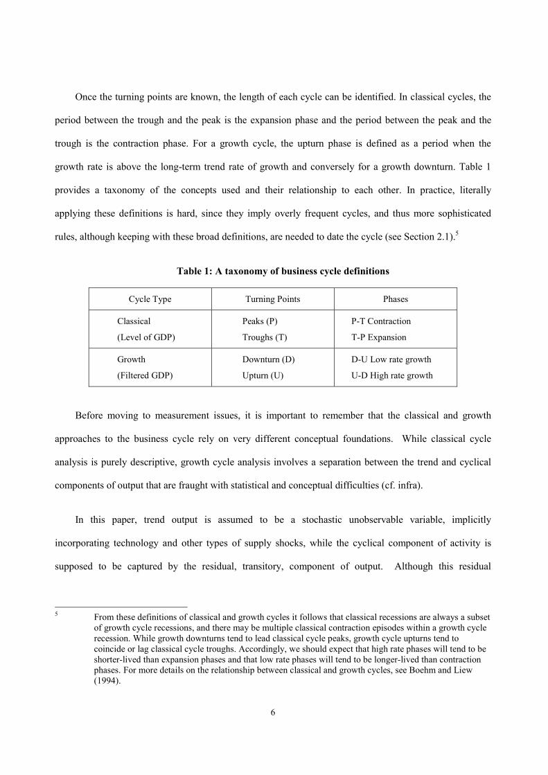
Once the turning points are known, the length of each cycle can be identified. In classical cycles, the

period between the trough and the peak is the expansion phase and the period between the peak and the

trough is the contraction phase. For a growth cycle, the upturn phase is defined as a period when the

growth rate is above the long-term trend rate of growth and conversely for a growth downturn. Table 1

provides a taxonomy of the concepts used and their relationship to each other. In practice, literally

applying these definitions is hard, since they imply overly frequent cycles, and thus more sophisticated

rules, although keeping with these broad definitions, are needed to date the cycle (see Section 2.1).5

Table 1: A taxonomy of business cycle definitions

Cycle Type Turning Points Phases

Classical

(Level of GDP)

Peaks (P)

Troughs (T)

P-T Contraction

T-P Expansion

Growth

(Filtered GDP)

Downturn (D)

Upturn (U)

D-U Low rate growth

U-D High rate growth

Before moving to measurement issues, it is important to remember that the classical and growth

approaches to the business cycle rely on very different conceptual foundations. While classical cycle

analysis is purely descriptive, growth cycle analysis involves a separation between the trend and cyclical

components of output that are fraught with statistical and conceptual difficulties (cf. infra).

In this paper, trend output is assumed to be a stochastic unobservable variable, implicitly

incorporating technology and other types of supply shocks, while the cyclical component of activity is

supposed to be captured by the residual, transitory, component of output. Although this residual

5 From these definitions of classical and growth cycles it follows that classical recessions are always a subset

of growth cycle recessions, and there may be multiple classical contraction episodes within a growth cycle recession. While growth downturns tend to lead classical cycle peaks, growth cycle upturns tend to coincide or lag classical cycle troughs. Accordingly, we should expect that high rate phases will tend to be shorter-lived than expansion phases and that low rate phases will tend to be longer-lived than contraction phases. For more details on the relationship between classical and growth cycles, see Boehm and Liew (1994).

7

component could include, in theory, transitory technology shocks, it is supposed to mainly capture

demand-driven fluctuations in output.6

A more “descriptive” approach, where trend output is approximated by a set of deterministic trends,

may have possibly allowed a more encompassing examination of cyclical fluctuations, including those

arising from the supply side. Emphasising, however, the demand side of the business cycle is not without

justification, given its centrality in the conduct of stabilisation policies. In short, using “real business

cycle” terminology, the paper leaves aside efficient supply-side fluctuations and focuses rather on

inefficient demand-driven cyclical fluctuations.

1.2 Measuring the growth cycle in OECD economies

Growth cycles are defined in terms of deviations from trend. The problem, however, is that trend

output growth cannot be directly measured. The rate of trend or potential growth is unobservable and has

to be inferred from the data. There are many possible approaches to decomposing a series into its trend and

cycle components and no single approach can claim to be unequivocally superior (see Box 1). Indeed, most

of the feasible approaches are ad hoc in the sense that the researcher requires only that the detrending

procedure produces a stationary business cycle component, but does not otherwise explicitly specify the

statistical characteristics of the business cycle. The choice of one methodology over another thus largely

hinges on the specific characteristics of the time series and the purpose of the analysis.

In this paper, to assess the main features of business cycles in OECD countries, we adopt a band-pass

filter, which is based on the idea that business cycles can be defined as fluctuations of a certain frequency.

The filter eliminates very slow moving (trend) components and very high frequency (irregular)

components while retaining intermediate (business cycle) components. When applying the filter, the

critical frequency band to be allocated to the cycle has to be exogenously determined. Here, we follow

Baxter and King (1999) and define the cycle using a uniform low pass filter to eliminate low frequency

6 This assumption would not be accepted by proponents of the Real Business Cycle school which tends to interpret the residual component as reflecting short-run supply fluctuations rather than demand-driven ones.

8

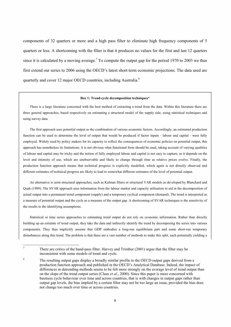
components of 32 quarters or more and a high pass filter to eliminate high frequency components of 5

quarters or less. A shortcoming with the filter is that it produces no values for the first and last 12 quarters

since it is calculated by a moving average.7 To compute the output gap for the period 1970 to 2003 we thus

first extend our series to 2006 using the OECD’s latest short-term economic projections. The data used are

quarterly and cover 12 major OECD countries, including Australia.8

Box 1: Trend-cycle decomposition techniques*

There is a large literature concerned with the best method of extracting a trend from the data. Within this literature there are

three general approaches, based respectively on estimating a structural model of the supply side, using statistical techniques and

using survey data.

The first approach uses potential output as the combination of various economic factors. Accordingly, an estimated production

function can be used to determine the level of output that would be produced if factor inputs - labour and capital - were fully

employed. Widely used by policy makers for its capacity to reflect the consequences of economic policies on potential output, this

approach has nonetheless its limitations: it is not obvious what functional form should be used, taking account of varying qualities

of labour and capital may be tricky and the notion of fully employed labour and capital is not easy to capture, as it depends on the

level and intensity of use, which are unobservable and likely to change through time as relative prices evolve. Finally, the

production function approach means that technical progress is explicitly modelled, which again is not directly observed and

different estimates of technical progress are likely to lead to somewhat different estimates of the level of potential output.

An alternative is semi-structural approaches, such as Kalman filters or structural VAR models as developed by Blanchard and

Quah (1989). The SVAR approach uses information from the labour market and capacity utilisation to aid in the decomposition of

actual output into a permanent trend component (supply) and a temporary cyclical component (demand). The trend is interpreted as

a measure of potential output and the cycle as a measure of the output gap. A shortcoming of SVAR techniques is the sensitivity of

the results to the identifying assumptions.

Statistical or time series approaches to estimating trend output do not rely on economic information. Rather than directly

building up an estimate of trend output, they take the data and indirectly identify the trend by decomposing the series into various

components. They thus implicitly assume that GDP embodies a long-run equilibrium part and some short-run temporary

disturbances along this trend. The problem is that there are a vast number of methods to make this split, each potentially yielding a

7 There are critics of the band-pass filter. Harvey and Trimbur (2001) argue that the filter may be

inconsistent with some models of trend and cycle. 8 The resulting output gaps display a broadly similar profile to the OECD output gaps derived from a

production function approach and published in the OECD’s Analytical Database. Indeed, the impact of differences in detrending methods seems to be felt more strongly on the average level of trend output than on the slope of the trend output series (Claus et al., 2000). Since this paper is more concerned with business cycle behaviour over time and across countries, that is with changes in output gaps rather than output gap levels, the bias implied by a certain filter may not be too large an issue, provided the bias does not change too much over time or across countries.

9

different dating of the turning points and growth cycle chronologies (Quah, 1992 and Canova, 1998). The simplest is to fit a linear

time trend and assume all deviations from the trend are cyclical. But this is likely to be unreliable during periods of structural

change as trend growth itself changes over time. Equally simple and avoiding a constant trend growth rate is to extrapolate a trend

between cyclical peaks, but in practice it can be complicated to implement because it requires a method to identify turning points.

The most frequently used approach is to apply time series techniques to extract the stochastic trend from GDP data. This

allows permanent movement in output as a result of shocks to aggregate supply. These techniques use various statistical criteria to

identify a trend. Examples include the perhaps most frequently used Hodrick Prescott filter (HP-filter), the band-pass filter, or the

Beveridge-Nelson decomposition. Each method requires some identifying assumptions, which are often criticized for their

arbitrariness and their lack of economic foundations. In practice, the differences across methods are typically small.

The third approach is to construct a measure of capacity utilisation based on business and household survey responses. These

responses can then be used to compile a measure of full capacity, with deviations representing cyclical fluctuations. Though this

approach is intuitively appealing, experience demonstrates that survey responses do not necessarily reflect aggregate demand

pressures, because respondents themselves seemingly find it hard to disentangle trend from cyclical developments.

All in all, estimating trend output remains an art more than a science and no single method can be said to be universally

superior. The choice of the preferred method remains therefore highly judgemental and dependent on the context and the objective

of the work.

* For a more detailed discussion, see the appendix in Cotis et al. (2004), on which this box is largely based.

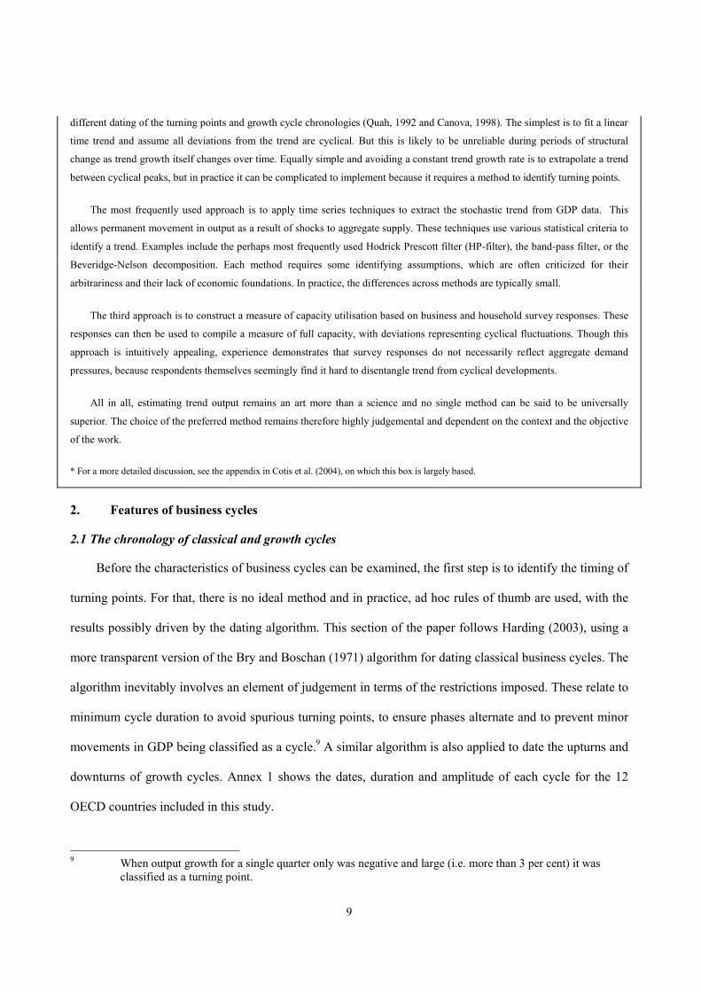
2. Features of business cycles

2.1 The chronology of classical and growth cycles

Before the characteristics of business cycles can be examined, the first step is to identify the timing of

turning points. For that, there is no ideal method and in practice, ad hoc rules of thumb are used, with the

results possibly driven by the dating algorithm. This section of the paper follows Harding (2003), using a

more transparent version of the Bry and Boschan (1971) algorithm for dating classical business cycles. The

algorithm inevitably involves an element of judgement in terms of the restrictions imposed. These relate to

minimum cycle duration to avoid spurious turning points, to ensure phases alternate and to prevent minor

movements in GDP being classified as a cycle.9 A similar algorithm is also applied to date the upturns and

downturns of growth cycles. Annex 1 shows the dates, duration and amplitude of each cycle for the 12

OECD countries included in this study.

9 When output growth for a single quarter only was negative and large (i.e. more than 3 per cent) it was

classified as a turning point.

10

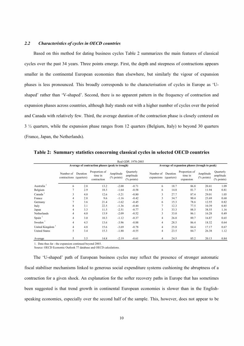
2.2 Characteristics of cycles in OECD countries

Based on this method for dating business cycles Table 2 summarizes the main features of classical

cycles over the past 34 years. Three points emerge. First, the depth and steepness of contractions appears

smaller in the continental European economies than elsewhere, but similarly the vigour of expansion

phases is less pronounced. This broadly corresponds to the characterisation of cycles in Europe as ‘U-

shaped’ rather than ‘V-shaped’. Second, there is no apparent pattern in the frequency of contraction and

expansion phases across countries, although Italy stands out with a higher number of cycles over the period

and Canada with relatively few. Third, the average duration of the contraction phase is closely centered on

3 ½ quarters, while the expansion phase ranges from 12 quarters (Belgium, Italy) to beyond 30 quarters

(France, Japan, the Netherlands).

Table 2: Summary statistics concerning classical cycles in selected OECD countries

Number of contractions

Duration (quarters)

Proportion of time in

contraction

Amplitude (% points)

Quarterly amplitude (% points)

Number of expansions

Duration (quarters)

Proportion of time in

expansion

Amplitude (% points)

Quarterly amplitude (% points)

Australia 1 6 2.8 13.2 -2.00 -0.71 6 18.7 86.8 20.41 1.09Belgium 7 2.9 18.3 -1.64 -0.58 6 14.8 81.7 11.94 0.81Canada 1 3 4.0 12.6 -3.21 -0.80 3 27.7 87.4 29.01 1.05France 4 2.8 9.6 -1.16 -0.42 3 34.7 90.4 23.69 0.68Germany 7 3.6 21.4 -1.62 -0.45 6 15.3 78.6 12.55 0.82Italy 8 3.1 22.5 -1.36 -0.44 7 12.3 77.5 10.39 0.85Japan 4 3.3 11.5 -2.51 -0.77 3 33.3 88.5 38.55 1.16Netherlands 4 4.0 13.9 -2.09 -0.52 3 33.0 86.1 16.28 0.49Spain 1 4 3.0 10.3 -1.12 -0.37 4 26.0 89.7 16.87 0.65Sweden 1 4 4.5 13.6 -3.96 -0.88 4 28.5 86.4 18.32 0.64United Kingdom 1 4 4.8 15.6 -3.69 -0.78 4 25.8 84.4 17.17 0.67United States 5 3.4 15.3 -1.88 -0.55 4 23.5 84.7 26.38 1.12

Average 5 3.5 14.8 -2.19 -0.61 4 24.5 85.2 20.13 0.84

1. Data thus far - the expansion continued beyond 2003.Source: OECD Economic Outlook 77 database and OECD calculations.

Average of expansion phases (trough to peak)Average of contraction phases (peak to trough)Real GDP, 1970-2003

The ‘U-shaped’ path of European business cycles may reflect the presence of stronger automatic

fiscal stabiliser mechanisms linked to generous social expenditure systems cushioning the abruptness of a

contraction for a given shock. An explanation for the softer recovery paths in Europe that has sometimes

been suggested is that trend growth in continental European economies is slower than in the English-

speaking economies, especially over the second half of the sample. This, however, does not appear to be

11

supported by Table 3, which shows the main features of growth cycles, abstracting from trend growth.

Indeed, all of the four countries where the average amplitude of upturns is below the 12-country average

are also euro area economies.

12

Table 3: Summary statistics concerning growth cycles in selected OECD countries

Number of downturns

Duration (quarters)

Proportion of time in

downturn

Amplitude (% points)

Quarterly amplitude (% points)

Number of upturns

Duration (quarters)

Proportion of time in upturn

Amplitude (% points)

Quarterly amplitude (% points)

Australia 7 6.3 37.0 3.51 0.56 7 10.7 63.0 3.34 0.31Belgium 10 5.9 48.4 2.55 0.43 10 6.3 51.6 2.61 0.41Canada 8 6.3 43.1 3.09 0.49 8 8.3 56.9 2.95 0.36France 6 8.3 46.7 2.35 0.28 6 9.5 53.3 2.23 0.23Germany 6 9.2 46.2 3.14 0.34 6 10.7 53.8 3.14 0.29Italy 9 6.1 45.1 3.09 0.51 9 7.4 54.9 3.04 0.41Japan 6 6.5 32.0 3.88 0.60 6 13.8 68.0 3.57 0.26Netherlands 7 6.4 37.2 2.58 0.40 7 10.9 62.8 2.66 0.25Spain 5 7.2 34.6 2.49 0.35 5 13.6 65.4 2.05 0.15Sweden 7 9.0 52.9 3.34 0.37 7 8.0 47.1 3.19 0.40United Kingdom 5 11.0 46.6 3.76 0.34 5 12.6 53.4 3.11 0.25United States 6 7.8 41.2 3.66 0.47 6 11.2 58.8 3.41 0.31

Average 7 7.5 42.6 3.12 0.43 7 10.2 57.4 2.94 0.30

Source: OECD Economic Outlook 77 database and OECD calculations.

Band-pass filtered real GDP, 1970-2003

Average downturns (downturn to upturn) Average upturns (upturn to downturn)

While the notion of cycle may implicitly convey a sense of regularity and repetition, the features of

growth cycles in OECD economies suggest anything but regularity. The length of upturn and downturn

phases ranges between 1 ½ and 3 ½ years and the steepness, or quarterly amplitude of cycles on average

spans a wide range. However, the cumulative magnitude of cycles, both during upturns and downturns is

relatively similar among countries.

Besides trying to identify country-specific cycles in OECD economies, we examined how the

output gap has evolved over time within and across countries. This approach shifts the focus away from

narrowly defined cycle analysis and takes a broader view of output fluctuations. On this basis, one feature

clearly evident in OECD economies over the past three decades is the drop in the amplitude of output

fluctuations, as proxied by the standard deviation of output gaps over approximately 9-year periods since

1970. The fall has been especially marked in the United States, Australia, the United Kingdom, as well as

Italy, Spain and Sweden and was heavily concentrated over the past decade. Also evident from Table 4 is a

tendency for the standard deviation of the output gap among the sampled countries to converge to a lower

level. On average over the last 9 years, the standard deviation of the output gap is about half what it was

during the 1970s.

13

Table 4: The amplitude of the business cycle has declined

Period 1 Period 2 Period 3 Period 4

Australia 1.01 1.77 1.42 0.62Belgium 1.39 1.05 1.01 0.88Canada 1.03 1.81 1.71 0.92France 1.01 0.75 0.91 0.89Germany 1.41 1.17 1.26 0.71Italy 1.92 1.14 1.00 0.62Japan 1.97 0.95 1.19 1.13Netherlands 0.93 1.33 0.93 0.89Spain 1.51 0.59 1.26 0.63Sweden 1.61 0.98 1.79 0.88United Kingdom 1.62 1.55 1.51 0.41United States 1.91 1.89 1.02 0.96

Euro area 1.20 0.85 0.94 0.68

Each period covers 35 quarters: Period 1: 1970q1-1978q3; Period 2: 1978q4-1987q2; Period 3: 1987q3-1996q1; Period 4: 1996q2-2004q4.

Source: OECD Economic Outlook 77 database and OECD calculations.

Standard deviation of the output gap, with trend GDP based on BP filter

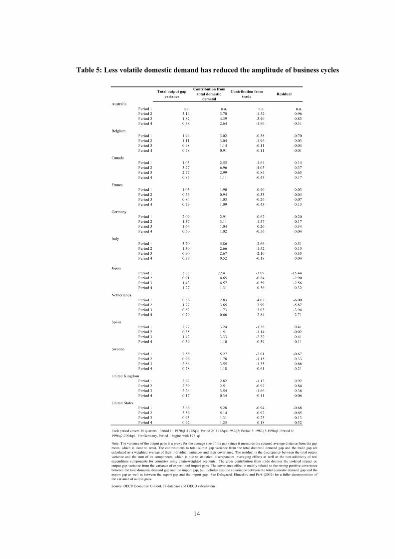
The tendency for the amplitude of the output gap to decline has been associated ex post with

reduced volatility of domestic demand as well as a smaller dampening influence from external trade (Table

5). Taken in isolation, the weakening contribution of trade to GDP smoothing may look paradoxical, in a

context where over the past 35 years trade openness has continuously increased. This modest contribution

to economic stabilisation may just signal, however, that in many countries domestic demand proved less

volatile and less susceptible to trigger equilibrating trade flows. Increased domestic demand stability may

partly reflect, in turn, improvements in the conduct of stabilisation policies, with monetary policy putting,

in particular, stronger emphasis on low and stable inflation. Moreover, as the relative size of the service

sector has increased and with technological innovations improving inventory management, the importance

of stock building to the cycle is less than it used to be.

14

Table 5: Less volatile domestic demand has reduced the amplitude of business cycles

Total output gap variance

Contribution from total domestic

demand

Contribution from trade Residual

AustraliaPeriod 1 n.a. n.a. n.a. n.a.Period 2 3.14 3.70 -1.52 0.96Period 3 1.82 4.39 -3.40 0.83Period 4 0.38 2.64 -1.96 -0.31

BelgiumPeriod 1 1.94 3.02 -0.38 -0.70Period 2 1.11 3.04 -1.96 0.03Period 3 0.98 1.14 -0.11 -0.04Period 4 0.78 0.91 -0.11 -0.01

CanadaPeriod 1 1.05 2.55 -1.64 0.14Period 2 3.27 6.96 -4.05 0.37Period 3 2.77 2.99 -0.84 0.63Period 4 0.85 1.11 -0.43 0.17

FrancePeriod 1 1.03 1.90 -0.90 0.03Period 2 0.56 0.94 -0.33 -0.04Period 3 0.84 1.03 -0.26 0.07Period 4 0.79 1.09 -0.43 0.13

GermanyPeriod 1 2.09 2.91 -0.62 -0.20Period 2 1.37 3.11 -1.57 -0.17Period 3 1.64 1.04 0.26 0.34Period 4 0.50 1.02 -0.56 0.04

ItalyPeriod 1 3.70 5.86 -2.66 0.51Period 2 1.30 2.66 -1.52 0.15Period 3 0.90 2.67 -2.10 0.33Period 4 0.39 0.52 -0.18 0.04

JapanPeriod 1 3.88 22.41 -3.09 -15.44Period 2 0.91 4.65 -0.84 -2.90Period 3 1.43 4.57 -0.59 -2.56Period 4 1.27 1.31 -0.36 0.32

NetherlandsPeriod 1 0.86 2.83 4.02 -6.00Period 2 1.77 3.65 3.99 -5.87Period 3 0.82 1.73 3.03 -3.94Period 4 0.79 0.66 2.84 -2.71

SpainPeriod 1 2.27 3.24 -1.38 0.41Period 2 0.35 1.51 -1.14 -0.02Period 3 1.42 3.33 -2.32 0.41Period 4 0.39 1.10 -0.59 -0.11

SwedenPeriod 1 2.58 5.27 -2.01 -0.67Period 2 0.96 1.78 -1.15 0.33Period 3 2.86 3.55 -1.35 0.66Period 4 0.78 1.18 -0.61 0.21

United KingdomPeriod 1 2.62 2.82 -1.13 0.92Period 2 2.39 2.51 -0.97 0.84Period 3 2.24 3.54 -1.66 0.36Period 4 0.17 0.34 -0.11 -0.06

United StatesPeriod 1 3.66 5.28 -0.94 -0.68Period 2 3.56 5.14 -0.92 -0.65Period 3 0.95 1.31 -0.23 -0.13Period 4 0.92 1.25 0.18 -0.52

Each period covers 35 quarters: Period 1: 1970q1-1978q3; Period 2: 1978q4-1987q2; Period 3: 1987q3-1996q1; Period 4: 1996q2-2004q4. For Germany, Period 1 begins with 1971q1.

Source: OECD Economic Outlook 77 database and OECD calculations.

Note: The variance of the output gaps is a proxy for the average size of the gap (since it measures the squared average distance from the gapmean, which is close to zero). The contributions to total output gap variance from the total domestic demand gap and the trade gap arecalculated as a weighted average of their individual variances and their covariance. The residual is the discrepancy between the total outputvariance and the sum of its components, which is due to statistical discrepancies, averaging effects as well as the non-additivity of realexpenditure components for countries using chain-weighted accounts. The gross contribution from trade denotes the isolated impact onoutput gap variance from the variance of export- and import gaps. The covariance effect is mainly related to the strong positive covariancebetween the total domestic demand gap and the import gap, but includes also the covariance between the total domestic demand gap and theexport gap as well as between the export gap and the import gap. See Dalsgaard, Elmeskov and Park (2002) for a fuller decomposition ofthe variance of output gaps.

15

2.3 Cross-country business cycle relationships in selected OECD countries

OECD economies have become increasingly integrated over the past half century, as trade and

investment agreements reduced barriers and improved the climate for cross-border commerce. Today, trade

openness in the OECD area is more than double the level in 1960 and foreign direct investment flows have

soared. Altogether, this might be expected to result in more similar cycles across countries in terms of their

intensity, duration and timing.

However, economic theory is not absolutely conclusive about the impact of increased trade on the

degree of business cycle synchronisation. Very often, international trade linkages generate both demand

and supply side spillovers across countries. For example, on the demand side an investment or

consumption boom in one country can generate increased demand for imports, boosting other economies.

Through these spillovers increased trade linkages result in more highly correlated business cycles. But

business cycle co-movement could weaken in cases where increased trade is associated with increased

inter-industry specialisation across countries and when industry-specific shocks are important in driving

business cycles.10

Of course, there are reasons why despite increased global integration, business cycles do not move in

tandem. Some economies are more susceptible to shocks than others. Economies, for instance, that are well

endowed with commodities, such as Australia, whose prices tend to fluctuate more widely than prices in

countries specialised in services, are more susceptible to wider cyclical movements. Moreover, even if a

shock is transmitted internationally, differences in the domestic structure of economies matters. How

quickly and at what cost an economy is able to absorb the shock varies, depending on the structure and

policy environment (see Section 3). Put succinctly, the degree to which the business cycle has become

synchronised across OECD economies is intrinsically an empirical issue.

10 See Kose and Yi (2002) for a discussion on trade linkages and co-movement.

16

In this section of the paper we, therefore, examine the statistical evidence for growth cycle

synchronisation, looking at three aspects: the timing of growth cycle turning points across countries, the

length of time cycles are in a similar phase with the cycle in the United States and the similarity of cycles

with respect to the intensity of output co-movement across countries.

2.3.1 The timing of the most recent cycle was closely synchronised

The simplest way to approach business cycle synchronisation is to compare turning point dates across

OECD countries. This can be achieved, based on the chronology of growth cycles, by examining the

density of national turning points at each point in time (Figure 1). A series of closely grouped turning

points is indicative of synchronisation. On this basis, there is no clear pattern toward greater or less

synchronisation in the timing of turning points. The one possible exception is the most recent downturn in

2001, which was prompted by a global shock. The recovery phase was also tightly grouped, though not all

countries in the sample participated in the recovery. Section 3.4 below examines the nature of the most

recent cycle compared with earlier ones and the differences in the forces driving recoveries across

countries.

17

Figure 1: The timing of growth cycle turning points is disperse

Source: OECD Economic Outlook 77 database and OECD calculations.

Downturn frequency

0

5

10

15

20

25

30

35

40

45

Per cent of countries

Upturn frequency

05

1015202530354045

1970

Q1

1971

Q1

1972

Q1

1973

Q1

1974

Q1

1975

Q1

1976

Q1

1977

Q1

1978

Q1

1979

Q1

1980

Q1

1981

Q1

1982

Q1

1983

Q1

1984

Q1

1985

Q1

1986

Q1

1987

Q1

1988

Q1

1989

Q1

1990

Q1

1991

Q1

1992

Q1

1993

Q1

1994

Q1

1995

Q1

1996

Q1

1997

Q1

1998

Q1

1999

Q1

2000

Q1

2001

Q1

2002

Q1

2003

Q1

2004

:Q1

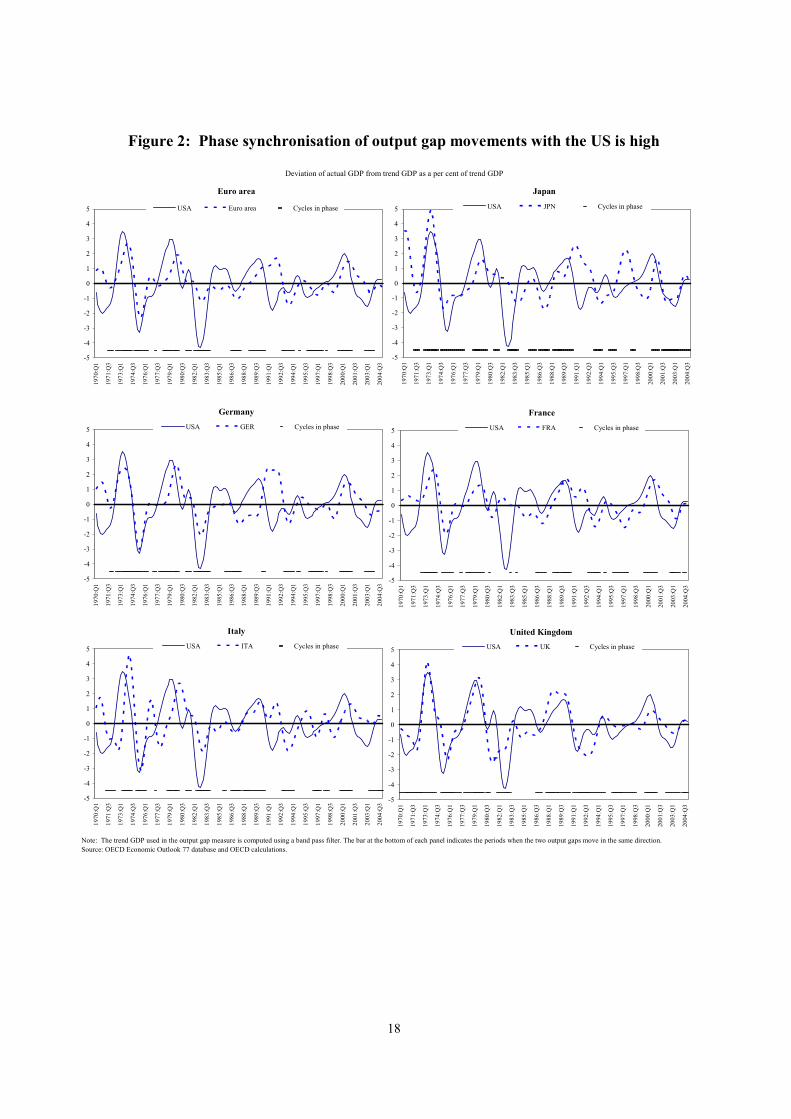
2.3.2 The duration of phase synchronisation with the US varies widely

Another aspect of business cycle synchronisation is the proportion of time two cycles are in the same

phase. Figure 2 plots movements in the output gap in each country as well as that for the Unites States. The

bar at the bottom of each panel indicates the periods when the two output gaps move in the same direction.

What is evident from the graphs is the higher proportion of time that Canada (75 per cent), Australia (62

per cent) and the United Kingdom (76 per cent) are in the same phase over the period 1970 to 2004,

compared with the euro area countries (56 per cent). The same calculations show that individual euro area

countries are much more often in phase with the euro area than the United States (not shown). In both

cases, there is no clear-cut trend towards increased phase synchronisation over time.

18

Figure 2: Phase synchronisation of output gap movements with the US is high

Note: The trend GDP used in the output gap measure is computed using a band pass filter. The bar at the bottom of each panel indicates the periods when the two output gaps move in the same direction. Source: OECD Economic Outlook 77 database and OECD calculations.

Deviation of actual GDP from trend GDP as a per cent of trend GDP

Japan

-5

-4

-3

-2

-1

0

1

2

3

4

5

1970

:Q1

1971

:Q3

1973

:Q1

1974

:Q3

1976

:Q1

1977

:Q3

1979

:Q1

1980

:Q3

1982

:Q1

1983

:Q3

1985

:Q1

1986

:Q3

1988

:Q1

1989

:Q3

1991

:Q1

1992

:Q3

1994

:Q1

1995

:Q3

1997

:Q1

1998

:Q3

2000

:Q1

2001

:Q3

2003

:Q1

2004

:Q3

USA JPN Cycles in phase

Germany

-5

-4

-3

-2

-1

0

1

2

3

4

5

1970

:Q1

1971

:Q3

1973

:Q1

1974

:Q3

1976

:Q1

1977

:Q3

1979

:Q1

1980

:Q3

1982

:Q1

1983

:Q3

1985

:Q1

1986

:Q3

1988

:Q1

1989

:Q3

1991

:Q1

1992

:Q3

1994

:Q1

1995

:Q3

1997

:Q1

1998

:Q3

2000

:Q1

2001

:Q3

2003

:Q1

2004

:Q3

USA GER Cycles in phase

France

-5

-4

-3

-2

-1

0

1

2

3

4

5

1970

:Q1

1971

:Q3

1973

:Q1

1974

:Q3

1976

:Q1

1977

:Q3

1979

:Q1

1980

:Q3

1982

:Q1

1983

:Q3

1985

:Q1

1986

:Q3

1988

:Q1

1989

:Q3

1991

:Q1

1992

:Q3

1994

:Q1

1995

:Q3

1997

:Q1

1998

:Q3

2000

:Q1

2001

:Q3

2003

:Q1

2004

:Q3

USA FRA Cycles in phase

Italy

-5

-4

-3

-2

-1

0

1

2

3

4

5

1970

:Q1

1971

:Q3

1973

:Q1

1974

:Q3

1976

:Q1

1977

:Q3

1979

:Q1

1980

:Q3

1982

:Q1

1983

:Q3

1985

:Q1

1986

:Q3

1988

:Q1

1989

:Q3

1991

:Q1

1992

:Q3

1994

:Q1

1995

:Q3

1997

:Q1

1998

:Q3

2000

:Q1

2001

:Q3

2003

:Q1

2004

:Q3

USA ITA Cycles in phase

United Kingdom

-5

-4

-3

-2

-1

0

1

2

3

4

5

1970

:Q1

1971

:Q3

1973

:Q1

1974

:Q3

1976

:Q1

1977

:Q3

1979

:Q1

1980

:Q3

1982

:Q1

1983

:Q3

1985

:Q1

1986

:Q3

1988

:Q1

1989

:Q3

1991

:Q1

1992

:Q3

1994

:Q1

1995

:Q3

1997

:Q1

1998

:Q3

2000

:Q1

2001

:Q3

2003

:Q1

2004

:Q3

USA UK Cycles in phase

Euro area

-5

-4

-3

-2

-1

0

1

2

3

4

5

1970

:Q1

1971

:Q3

1973

:Q1

1974

:Q3

1976

:Q1

1977

:Q3

1979

:Q1

1980

:Q3

1982

:Q1

1983

:Q3

1985

:Q1

1986

:Q3

1988

:Q1

1989

:Q3

1991

:Q1

1992

:Q3

1994

:Q1

1995

:Q3

1997

:Q1

1998

:Q3

2000

:Q1

2001

:Q3

2003

:Q1

2004

:Q3

USA Euro area Cycles in phase

19

Figure 2: Phase synchronisation of output gap movements with the US is high, continued

Note: The trend GDP used in the output gap measure is computed using a band pass filter. The bar at the bottom of each panel indicates the periods when the two output gaps move in the same direction. Source: OECD Economic Outlook 77 database and OECD calculations.

Deviation of actual GDP from trend GDP as a per cent of trend GDP

Canada

-5

-4

-3

-2

-1

0

1

2

3

4

5

1970

:Q1

1971

:Q3

1973

:Q1

1974

:Q3

1976

:Q1

1977

:Q3

1979

:Q1

1980

:Q3

1982

:Q1

1983

:Q3

1985

:Q1

1986

:Q3

1988

:Q1

1989

:Q3

1991

:Q1

1992

:Q3

1994

:Q1

1995

:Q3

1997

:Q1

1998

:Q3

2000

:Q1

2001

:Q3

2003

:Q1

2004

:Q3

USA CAN Cycles in phase

Australia

-5

-4

-3

-2

-1

0

1

2

3

4

5

1970

:Q1

1971

:Q3

1973

:Q1

1974

:Q3

1976

:Q1

1977

:Q3

1979

:Q1

1980

:Q3

1982

:Q1

1983

:Q3

1985

:Q1

1986

:Q3

1988

:Q1

1989

:Q3

1991

:Q1

1992

:Q3

1994

:Q1

1995

:Q3

1997

:Q1

1998

:Q3

2000

:Q1

2001

:Q3

2003

:Q1

2004

:Q3

USA AUS Cycles in phase

Belgium

-5

-4

-3

-2

-1

0

1

2

3

4

5

1970

:Q1

1971

:Q3

1973

:Q1

1974

:Q3

1976

:Q1

1977

:Q3

1979

:Q1

1980

:Q3

1982

:Q1

1983

:Q3

1985

:Q1

1986

:Q3

1988

:Q1

1989

:Q3

1991

:Q1

1992

:Q3

1994

:Q1

1995

:Q3

1997

:Q1

1998

:Q3

2000

:Q1

2001

:Q3

2003

:Q1

2004

:Q3

USA BEL Cycles in phase

Netherlands

-5

-4

-3

-2

-1

0

1

2

3

4

519

70:Q

1

1971

:Q3

1973

:Q1

1974

:Q3

1976

:Q1

1977

:Q3

1979

:Q1

1980

:Q3

1982

:Q1

1983

:Q3

1985

:Q1

1986

:Q3

1988

:Q1

1989

:Q3

1991

:Q1

1992

:Q3

1994

:Q1

1995

:Q3

1997

:Q1

1998

:Q3

2000

:Q1

2001

:Q3

2003

:Q1

2004

:Q3

USA NLD Cycles in phase

Spain

-5

-4

-3

-2

-1

0

1

2

3

4

5

1970

:Q1

1971

:Q3

1973

:Q1

1974

:Q3

1976

:Q1

1977

:Q3

1979

:Q1

1980

:Q3

1982

:Q1

1983

:Q3

1985

:Q1

1986

:Q3

1988

:Q1

1989

:Q3

1991

:Q1

1992

:Q3

1994

:Q1

1995

:Q3

1997

:Q1

1998

:Q3

2000

:Q1

2001

:Q3

2003

:Q1

2004

:Q3

USA SPA Cycles in phase

Sweden

-5

-4

-3

-2

-1

0

1

2

3

4

5

1970

:Q1

1971

:Q3

1973

:Q1

1974

:Q3

1976

:Q1

1977

:Q3

1979

:Q1

1980

:Q3

1982

:Q1

1983

:Q3

1985

:Q1

1986

:Q3

1988

:Q1

1989

:Q3

1991

:Q1

1992

:Q3

1994

:Q1

1995

:Q3

1997

:Q1

1998

:Q3

2000

:Q1

2001

:Q3

2003

:Q1

2004

:Q3

USA SWE Cycles in phase

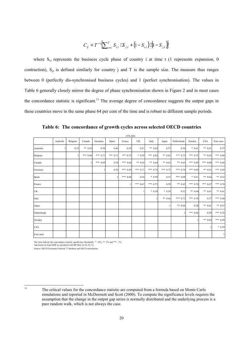
We also examined whether the above stylized facts were corroborated using the statistical framework

suggested by Harding and Pagan (2002) (Table 6). They propose examining the degree of concordance

between two cycles using the measure:

20

( ) ( ){ }tjtiT

t tjtiij SSSSTC ,,1 ,,1 11 −⋅−+⋅= ∑ =

−

where Si,t represents the business cycle phase of country i at time t (1 represents expansion, 0

contraction), Sj,t is defined similarly for country j and T is the sample size. The measure thus ranges

between 0 (perfectly dis-synchronised business cycles) and 1 (perfect synchronisation). The values in

Table 6 generally closely mirror the degree of phase synchronisation shown in Figure 2 and in most cases

the concordance statistic is significant.11 The average degree of concordance suggests the output gaps in

these countries move in the same phase 64 per cent of the time and is robust to different sample periods.

Table 6: The concordance of growth cycles across selected OECD countries

Australia Belgium Canada Germany Spain France UK Italy Japan Netherlands Sweden USA Euro area

Australia 1 0.53 ** 0.65 0.54 0.46 0.55 0.51 ** 0.65 0.57 0.54 * 0.61 ** 0.61 0.57

Belgium 1 *** 0.68 *** 0.71 *** 0.71 *** 0.75 * 0.59 *** 0.82 ** 0.63 *** 0.73 *** 0.75 ** 0.65 *** 0.80

Canada 1 *** 0.69 0.58 *** 0.66 ** 0.64 ** 0.64 ** 0.62 ** 0.65 *** 0.69 *** 0.80 *** 0.66

Germany 1 0.56 *** 0.69 *** 0.71 *** 0.74 *** 0.75 *** 0.74 *** 0.69 ** 0.61 *** 0.85

Spain 1 *** 0.66 0.54 * 0.59 0.53 *** 0.69 * 0.61 ** 0.64 ** 0.63

France 1 *** 0.67 *** 0.73 0.59 ** 0.65 *** 0.70 *** 0.67 *** 0.74

UK 1 * 0.59 * 0.58 0.52 ** 0.64 ** 0.61 ** 0.61

Italy 1 ** 0.66 *** 0.72 *** 0.70 0.57 *** 0.88

Japan 1 ** 0.66 0.58 ** 0.61 ** 0.67

Netherlands 1 *** 0.66 0.58 *** 0.76

Sweden 1 ** 0.64 *** 0.69

USA 1 * 0.59

Euro area 1

The stars indicate the concordance statistic significance thresholds: * :10%, **: 5% and *** : 1%.Gap based on trend GDP as calculated with BP filter (6,32), K=12.Source: OECD Economic Outlook 77 database and OECD calculations.

1970-2004

11 The critical values for the concordance statistic are computed from a formula based on Monte Carlo

simulations and reported in McDermott and Scott (2000). To compute the significance levels requires the assumption that the change in the output gap series is normally distributed and the underlying process is a pure random walk, which is not always the case.

21

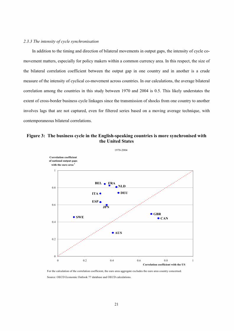
2.3.3 The intensity of cycle synchronisation

In addition to the timing and direction of bilateral movements in output gaps, the intensity of cycle co-

movement matters, especially for policy makers within a common currency area. In this respect, the size of

the bilateral correlation coefficient between the output gap in one country and in another is a crude

measure of the intensity of cyclical co-movement across countries. In our calculations, the average bilateral

correlation among the countries in this study between 1970 and 2004 is 0.5. This likely understates the

extent of cross-border business cycle linkages since the transmission of shocks from one country to another

involves lags that are not captured, even for filtered series based on a moving average technique, with

contemporaneous bilateral correlations.

Figure 3: The business cycle in the English-speaking countries is more synchronised with the United States

For the calculation of the correlation coefficient, the euro area aggregate excludes the euro area country concerned.

Source: OECD Economic Outlook 77 database and OECD calculations.

1970-2004

AUS

BEL

CAN

DEU

ESP

FRA

GBR

ITA

JPN

NLD

SWE

0

0.2

0.4

0.6

0.8

1

0 0.2 0.4 0.6 0.8 1Correlation coefficient with the US

Correlation coefficient of national output gaps

with the euro area 1

22

Generally, the euro zone countries are more highly correlated with the rest of the euro area (i.e.

excluding the euro zone country from the euro area) than the United States. In contrast, Australia’s and

Canada’s cycles are relatively more closely synchronised with the United States (Figure 3). The United

Kingdom’s greater correlation with the United States than the euro area appears puzzling, given the

country’s close economic ties with the euro area. However, the correlation coefficient mixes characteristics

of duration and amplitude into one measure and common shifts in amplitude may be hard to interpret in

terms of diffusion and propagation of output fluctuations. An example of such ambiguity may occur when

for autonomous reasons – i.e. universally improved stabilisation policies – countries share a common trend

of decreasing output volatility.

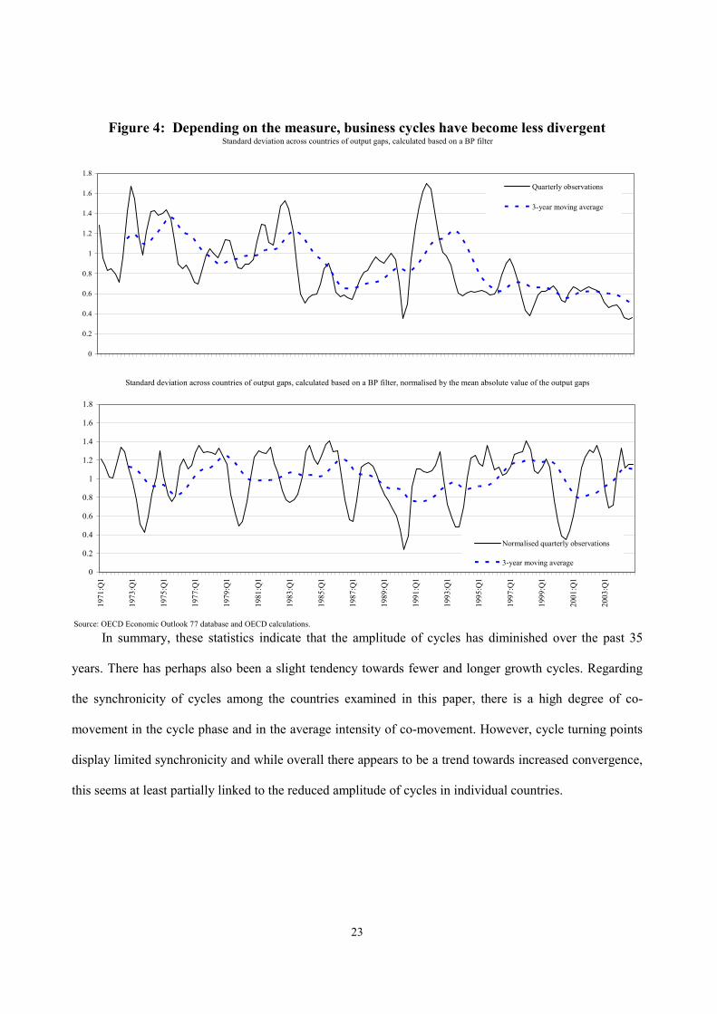
The above measures provide a sense of business cycle convergence on average over the period. But

they are not well suited to gauge whether synchronisation – in the sense of propagation – has risen over

time. Stronger propagation seems likely, however, not least given the increased size of household and

corporate balance sheets, with assets whose prices are determined in world markets. One proxy for

measuring the changing degree of cycle synchronisation is to examine how the standard deviation of output

gaps across countries has evolved. If this measure were consistently zero over time, it would indicate that

business cycles in the 12 countries in this study have the same timing and amplitude. On this basis, there is

certainly a clear trend towards less divergent cycles over time (Figure 4, top panel).

However, since other measures of cyclical convergence (timing of turning points, proportion of time

in same phase of the cycle) do not suggest a clear-cut trend toward increased synchronisation, the reduction

in output gap dispersion is also likely to reflect the fact that output gaps on average have become smaller

over time. Indeed, when the standard deviation across countries of output gaps is normalized by the

average absolute value of the gap to control for the effect of smaller gaps there is no clear downward trend

over time (Figure 4, bottom panel).

23

Figure 4: Depending on the measure, business cycles have become less divergent

Source: OECD Economic Outlook 77 database and OECD calculations.

Standard deviation across countries of output gaps, calculated based on a BP filter, normalised by the mean absolute value of the output gaps

Standard deviation across countries of output gaps, calculated based on a BP filter

0

0.2

0.4

0.6

0.8

1

1.2

1.4

1.6

1.8

Quarterly observations

3-year moving average

0

0.2

0.4

0.6

0.8

1

1.2

1.4

1.6

1.8

1971

:Q1

1973

:Q1

1975

:Q1

1977

:Q1

1979

:Q1

1981

:Q1

1983

:Q1

1985

:Q1

1987

:Q1

1989

:Q1

1991

:Q1

1993

:Q1

1995

:Q1

1997

:Q1

1999

:Q1

2001

:Q1

2003

:Q1

Normalised quarterly observations

3-year moving average

In summary, these statistics indicate that the amplitude of cycles has diminished over the past 35

years. There has perhaps also been a slight tendency towards fewer and longer growth cycles. Regarding

the synchronicity of cycles among the countries examined in this paper, there is a high degree of co-

movement in the cycle phase and in the average intensity of co-movement. However, cycle turning points

display limited synchronicity and while overall there appears to be a trend towards increased convergence,

this seems at least partially linked to the reduced amplitude of cycles in individual countries.

24

3 Forces bearing on OECD business cycle dynamics

3.1 Sources of divergence in the current cycle

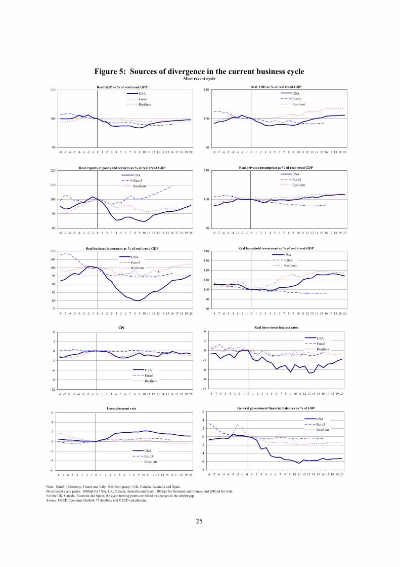
What is striking with the volatility statistics discussed above is they don’t clearly suggest that

current characteristics of the cycle are notably different across OECD countries despite the now

widespread perception that a group of ‘successful’ countries (Australia, Canada, Ireland, New Zealand,

Nordic countries and the United Kingdom) did much better than average to weather the 2001 global

slowdown, while large continental European countries seem mired in a low activity trap. Such a

discrepancy may reflect the difficulties encountered by statistical filters to distinguish between persistently

weak demand and lower trend output, especially at end of sample. By contrast, volatility statistics

computed with OECD traditional production function based, trend output yield a somewhat different

picture and are closer to intuition (Figure 5).

This picture is one of distinct resilience (i.e. avoiding long periods away from equilibrium

following negative shocks) in the successful group in reaction to the 2001 slowdown. Even though the

downturn in all countries was to a large extent prompted by a worldwide demand shock related to the

bursting of bubbles in equity prices and over-investment in ICT equipment, growth relative to trend barely

slowed in Australia, Canada, the UK, Spain and some others, whereas the large continental European

economies, and hence the euro area as a whole, faced a protracted slowdown. Furthermore, the pace of

recovery remains more subdued in the euro area, with the output gap projected to widen further before

starting to close very slowly over the next two years.

25

Figure 5: Sources of divergence in the current business cycle

Note: Euro3 = Germany, France and Italy. Resilient group = UK, Canada, Australia and Spain.Most recent cycle peaks: 2000q4 for USA, UK, Canada, Australia and Spain; 2002q3 for Germany and France; and 2002q4 for Italy. For the UK, Canada, Australia and Spain, the cycle turning points are based on changes in the output gap.Source: OECD Economic Outlook 77 database and OECD calculations.

Most recent cycle

Real GDP as % of real trend GDP

90

100

110

-8 -7 -6 -5 -4 -3 -2 -1 0 1 2 3 4 5 6 7 8 9 10 11 12 13 14 15 16 17 18 19 20

USAEuro3Resilient

Real TDD as % of real trend GDP

90

100

110

-8 -7 -6 -5 -4 -3 -2 -1 0 1 2 3 4 5 6 7 8 9 10 11 12 13 14 15 16 17 18 19 20

USAEuro3Resilient

Real exports of goods and services as % of real trend GDP

80

90

100

110

120

-8 -7 -6 -5 -4 -3 -2 -1 0 1 2 3 4 5 6 7 8 9 10 11 12 13 14 15 16 17 18 19 20

USAEuro3Resilient

Real private consumption as % of real trend GDP

90

100

110

-8 -7 -6 -5 -4 -3 -2 -1 0 1 2 3 4 5 6 7 8 9 10 11 12 13 14 15 16 17 18 19 20

USAEuro3Resilient

Real business investment as % of real trend GDP

75

80

85

90

95

100

105

110

-8 -7 -6 -5 -4 -3 -2 -1 0 1 2 3 4 5 6 7 8 9 10 11 12 13 14 15 16 17 18 19 20

USAEuro3Resilient

Real household investment as % of real trend GDP

80

90

100

110

120

130

140

-8 -7 -6 -5 -4 -3 -2 -1 0 1 2 3 4 5 6 7 8 9 10 11 12 13 14 15 16 17 18 19 20

USAEuro3Resilient

CPI

-12

-9

-6

-3

0

3

6

-8 -7 -6 -5 -4 -3 -2 -1 0 1 2 3 4 5 6 7 8 9 10 11 12 13 14 15 16 17 18 19 20

USAEuro3Resilient

Real short-term interest rates

-12

-9

-6

-3

0

3

6

-8 -7 -6 -5 -4 -3 -2 -1 0 1 2 3 4 5 6 7 8 9 10 11 12 13 14 15 16 17 18 19 20

USAEuro3Resilient

Unemployment rate

-6

-4

-2

0

2

4

6

-8 -7 -6 -5 -4 -3 -2 -1 0 1 2 3 4 5 6 7 8 9 10 11 12 13 14 15 16 17 18 19 20

USAEuro3Resilient

General government financial balances as % of GDP

-8

-6

-4

-2

0

2

4

6

-8 -7 -6 -5 -4 -3 -2 -1 0 1 2 3 4 5 6 7 8 9 10 11 12 13 14 15 16 17 18 19 20

USAEuro3Resilient

26

The current situation with the English speaking and Nordic countries faring well stands in stark

contrast with the experience of previous slowdowns where these same economies showed fragility during

the slowdown and lack of responsiveness in the upswing (Figure 6). On the contrary, developments in the

euro area are similar to previous cycles, suggesting that its relatively lower degree of resilience does not

represent an entirely new phenomenon.

A notable difference across country groups in the current cycle has been the behaviour of private

consumption and residential investment. In stark contrast with previous episodes, these have shown

strength both in the United States and in the successful economies, offsetting weakness in the more

externally exposed sectors. In contrast, household demand in the euro area failed to buffer the slowdown

and support recovery in line with past experience. Moreover, it appears that these differences can only be

partly attributed to disparities in the stance of macroeconomic policy, since a similar aggregate response of

monetary and to a somewhat lesser degree fiscal policies was observed in both groups of countries (see

Figure 5, lower two right hand panels).12 This suggests that more fundamental or structural factors are

behind divergences in the capacity of the economies to absorb and recover from shocks, including

differences in the effectiveness of macroeconomic policies, especially through their influence on domestic

demand. The following section examines some of the underlying causes of those differences in the

capacity to absorb adverse shocks and speedily recover in their aftermath.

12 If exchange rate developments are taken into consideration, then euro area monetary conditions hardly

changed.

27

Figure 6: Sources of divergence in the previous business cycle

Note: Euro3 = Germany, France and Italy. Resilient group = UK, Canada, Australia and Spain.Previous cycle peaks: 1990q2 for USA, UK and Australia; 1992q2 for Germany, France, Italy and Spain; and 1990q1 for Canada.Source: OECD Economic Outlook 77 database and OECD calculations.

Previous cycle

Real GDP as % of real trend GDP

90

100

110

-8 -7 -6 -5 -4 -3 -2 -1 0 1 2 3 4 5 6 7 8 9 10 11 12 13 14 15 16 17 18 19 20

USAEuro3Resilient

Real TDD as % of real trend GDP

90

100

110

-8 -7 -6 -5 -4 -3 -2 -1 0 1 2 3 4 5 6 7 8 9 10 11 12 13 14 15 16 17 18 19 20

USAEuro3Resilient

Real exports of goods and services as % of real trend GDP

80

90

100

110

120

-8 -7 -6 -5 -4 -3 -2 -1 0 1 2 3 4 5 6 7 8 9 10 11 12 13 14 15 16 17 18 19 20

USAEuro3Resilient

Real private consumption as % of real trend GDP

90

100

110

-8 -7 -6 -5 -4 -3 -2 -1 0 1 2 3 4 5 6 7 8 9 10 11 12 13 14 15 16 17 18 19 20

USAEuro3Resilient

Real business investment as % of real trend GDP

75

80

85

90

95

100

105

110

-8 -7 -6 -5 -4 -3 -2 -1 0 1 2 3 4 5 6 7 8 9 10 11 12 13 14 15 16 17 18 19 20

USAEuro3Resilient

Real household investment as % of real trend GDP

80

90

100

110

120

-8 -7 -6 -5 -4 -3 -2 -1 0 1 2 3 4 5 6 7 8 9 10 11 12 13 14 15 16 17 18 19 20

USAEuro3Resilient

CPI

-12

-9

-6

-3

0

3

6

-8 -7 -6 -5 -4 -3 -2 -1 0 1 2 3 4 5 6 7 8 9 10 11 12 13 14 15 16 17 18 19 20

USAEuro3Resilient

Real short-term interest rates

-12

-9

-6

-3

0

3

6

-8 -7 -6 -5 -4 -3 -2 -1 0 1 2 3 4 5 6 7 8 9 10 11 12 13 14 15 16 17 18 19 20

USAEuro3Resilient

Unemployment rate

-6

-4

-2

0

2

4

6

-8 -7 -6 -5 -4 -3 -2 -1 0 1 2 3 4 5 6 7 8 9 10 11 12 13 14 15 16 17 18 19 20

USAEuro3Resilient

General government financial balances as % of GDP

-8

-6

-4

-2

0

2

4

6

-8 -7 -6 -5 -4 -3 -2 -1 0 1 2 3 4 5 6 7 8 9 10 11 12 13 14 15 16 17 18 19 20

USAEuro3Resilient

28

3.2 Why did successful economies become more resilient?

3.2.1 A hypothesis that attributes strong resilience to good structural policies

There are a number of possible linkages between structural policies, growth and resilience that can be

invoked to explain how strong long-term growth may also increase short-term adaptability to shocks.

These include:

• Structural regulatory settings that serve to accelerate the speed of real wage adjustment and to

reduce unemployment persistence.13 This will generally lead to shorter deviations of actual

output and employment from equilibrium.14 Also, faster reversals of unemployment to

equilibrium reduce the risk that hysteresis effects set in and therefore that adverse shocks will

permanently lower employment rates.

• Regulatory settings favourable to the development of financial markets, because they also

contribute to greater consumption smoothing by providing households with better access to

credit markets, allowing them to borrow against the least liquid component of their wealth,

i.e. housing.15 As well, it is likely that flexible and diversified financial markets tend to

strengthen the elasticity of domestic and household demand to interest rates (see Section 3.2.2

below).

• Flexible product and labour market regulations could speed the recovery process following an

adverse shock to the extent that factor reallocation is enhanced. Moreover, by facilitating the

process of creative destruction, light regulation may enhance the expansion phase once it

takes hold.16

• Labour market policies that lead to low structural unemployment and short unemployment

duration spells tend to reduce precautionary saving.

To illustrate the effect of flexible labour, product and capital markets and strong monetary policy

transmission mechanisms on the degree of resilience of economies, recent OECD work developed a small

13 Differences in structural policy and institutions, to the extent they imply differences in the speed of real

wage adjustment across countries have been identified as one of the reasons why a number of large common shocks in the 1970s and 1980s led to diverse unemployment experiences across countries. See, for example, Blanchard and Wolfers (2000); Bertola et al. (2002), Fitoussi et al. (2000) and OECD (1994).

14 It is equally possible that the deviations are shallower, depending on the source of the shocks. 15 See, for example, Catte et al. (2004). 16 See, for instance, Bergoeing et al. (2002), Caballero and Hammour (2000) and Davis et al. (1996).

29

simulation model with alternative calibrations to replicate economic structures in the US and the euro

area.17 The US model is able to replicate the key properties of the Federal Reserve Board’s FRB-US

model of the US economy. However, for the euro area model to display similar properties shown by the

ECB’s Area-Wide Model it was necessary to incorporate changes to reflect rigidities in product and labour

markets. This was done by lengthening lag structures in price and wage setting and by reducing the impact

that any disequilibria have on behaviour. Once calibrated to capture the general workings of the US and

euro area economies, these macquettes can be used to simulate the economic consequences of various

shocks. The results broadly suggest that an economy characterised by rigidities tends to be less resilient.

3.2.2 OECD empirical work tentatively supports a relationship between price rigidities and regulatory settings

There is empirical support for the notion that structural policies and institutions in the euro area

prolong adjustment and bear adversely on the effectiveness of monetary policy. Concerning, for example,

the length of time to adjust to a shock, OECD work has examined why consumer price inflation in the euro

area has remained persistently above the ECB’s 2 per cent objective even through periods when the output

gap was clearly negative.18 In contrast, prices seem to adjust upwards in a normal manner when capacity

constraints are evident.

The responsiveness of prices to output developments was thus examined by estimating an asymmetric

Philips curve for a panel of 17 OECD countries, including various non-euro area economies. Apart from

linking inflation to a measure of inflation expectations and the output gap,19 the model included an

interaction term with the output gap to capture the effects of structural rigidities on the cycle. The rigidity

indicators used in the regressions were the strength of employment protection legislation and the tightness

of product market regulations.20 The model was estimated with quarterly data over the period 1985Q1 to

2004Q4 using Panel Ordinary Least Squares.

The main result from the analysis is a statistically significant link between more rigid regulatory

settings and a weaker response of prices to a negative output gap. Since the euro area countries score

higher on these measures of structural rigidity than the English-speaking countries in the sample the

17 See Drew et al. (2004). 18 See Cournède et al. (2005). 19 The output gap series is from the OECD’s Analytical Database. Robustness of the regression results were

examined, inter alia, using a univariate estimate of the output gap. 20 The structural policy variables were defined on a 0-5 scale, with higher values corresponding to stricter

regulation, or more centralised wage coordination. The degree of concentration in wage bargaining was also examined, but the estimation results were less convincing.

30

simulated response of inflation to a widening negative output gap is much weaker in most of the euro area

(Table 7).

Table 7: The impact of slack on inflation

Simulated inflation fall induced by a 1 percentage point wider negative output gap1

Structural indicator used in the regression

Employment protection legislation

Product market regulation

Euro area countries Austria 0.1 0.2 Belgium 0.4 0.2 Finland 0.2 0.3 France 0.2 0.1 Germany 0.1 0.3 Italy 0.4 0.1 Netherlands 0.0 0.2 Spain 0.0 0.2

Other countries Australia 0.5 0.3 Canada 0.5 0.4 Denmark 0.4 0.2 Japan 0.2 0.3 New Zealand 0.5 0.3 Norway 0.0 0.2 Sweden 0.1 0.3 United Kingdom 0.6 0.4 United States 0.8 0.4

1. Inflation relates to the annualised quarterly change in the consumer price index. The sources for the data and indicators underlying the calculations are described in Cournède et al. (2005). The results shown here are based on the coefficients drawn from regressing inflation on the previous period output gap, on its interaction with the corresponding rigidity index, on expected inflation and on other variables.

This result implies the sacrifice ratio in the ‘rigid’ euro area is larger than in the ‘flexible’ English-

speaking countries. Another dimension to resilience, also influencing the size of the sacrifice ratio, is the

speed and magnitude with which monetary policy responses to shocks are transmitted through economies.

In this regard, other recent OECD work has examined whether the structure of housing and mortgage

markets influences the effectiveness of monetary policy.21 The focus on the housing market is not

accidental. It is motivated by the stylised fact, observed above, that a source of divergence across countries

in the current cycle relates to the behaviour of residential investment.

21 See Catte et al. (2004).

31

The study finds a strong linkage from house prices to activity through wealth channels affecting

personal consumption, in line with other research.22 Housing markets are also important in the transmission

of monetary policy. A high interest rate sensitivity is beneficial as it implies that monetary policy is more

powerful in boosting or damping cyclical fluctuations. But the effects of monetary policy on activity, as

measured by the impact of policy-determined interest rate changes on housing market interest rates and

then on house prices and wealth differ considerably across OECD economies. These differences in the size

and speed of interaction between housing and the business cycle can be partly traced back to differences in

institutional features of housing and mortgage markets, such as the type of mortgage interest regime that

predominates (i.e. floating or fixed) and the costs of refinancing (Table 8). Those countries where the

degree of mortgage market ‘completeness’ is high23 are associated with a larger estimated long-term

marginal propensity to consume out of housing wealth. This suggests that the mortgage market is pivotal in

translating house price shocks into spending responses. Indeed, the close relationship of mortgage market

‘completeness’ with real house price-consumption correlations and housing equity withdrawal illustrates

the crucial role played by the provision of liquidity in connection with housing assets (Figure 7).24

22 See for example, Pichette and Tremblay (2003) for Canada, Case et al. (2001) and Benjamin et al. (2003)

for the United States, Deutsche Bundesbank (2003) for Germany, OECD (2003b) for the United Kingdom, Dvornak and Kohler (2003) for Australia and Ludwig and Sløk (2004) for a panel of seven countries.

23 See Mercer, Oliver and Wyman (2003) for details on the compilation of the index. The index is calculated for the eight countries shown in Table 8.

24 More generally, ongoing work at the OECD is examining the linkages between financial market development and output growth.

32

Table 8: Mortgage market completeness: range of mortgage products available and of borrowers served in eight European countries

Denmark France Germany Italy Netherlands Portugal SpainUnited

Kingdom

a) LTV ratios Typical 80 67 67 55 90 83 70 69Maximum 80 100 80 80 115 90 100 110b) Variety of mortgage productsRate structure Variable ** ** ** ** ** ** ** **Variable (referenced) ** ** - ** ** ** ** **Discounted - ** - * - - ** **Capped ** ** * * ** - * **Range of fixed terms 2-5 ** ** ** ** ** * * **5-10 ** ** ** ** ** * * *10-20 ** ** ** * ** - * *20+ ** * * * * - * - Repayment structures Amortising ** ** ** ** ** ** ** **Interest only * ** ** * ** - - **Flexible * ** - * ** - * **Fee-free redemption a ** - - - - - - *Full yield maintenance fee ** * ** * ** * * *c) Range of borrower types and mortgage purposes Borrower type Young household (<30) ** * ** * * ** ** **Older household (>50) ** * * * ** * * **Low equity - ** * - * * * **Self-certify income - - - - * - * *Previously bankrupt * - - - - - - *Credit impaired * * - * * - * **Self employed ** * ** ** * ** ** **Government sponsored * ** * * * ** * *Purpose of loan Second mortgage ** * ** ** ** ** ** **Overseas holiday homes ** ** * ** * - - **Rental ** ** ** ** ** ** ** **Equity release ** - * ** ** - * **Shared ownership ** * * * * ** - **Mortgage market completeness index b 75 72 58 57 79 47 66 86

Note: Readily available means that products are actively marketed with high public awareness; Limited availability means that only a small subset of lenders provide this

Key: ** Readily available * Limited availability - No availabilitya) On fixed-rate products only. b) See Mercer Oliver Wyman (2003) for details on the calculation of the index.Source: Mercer Oliver Wyman (2003).

product, often with additional conditions; No availability means that no lenders surveyed offered the product. See Mercer Oliver Wyman (2003) for further details on the sample and criteria of the survey.

33

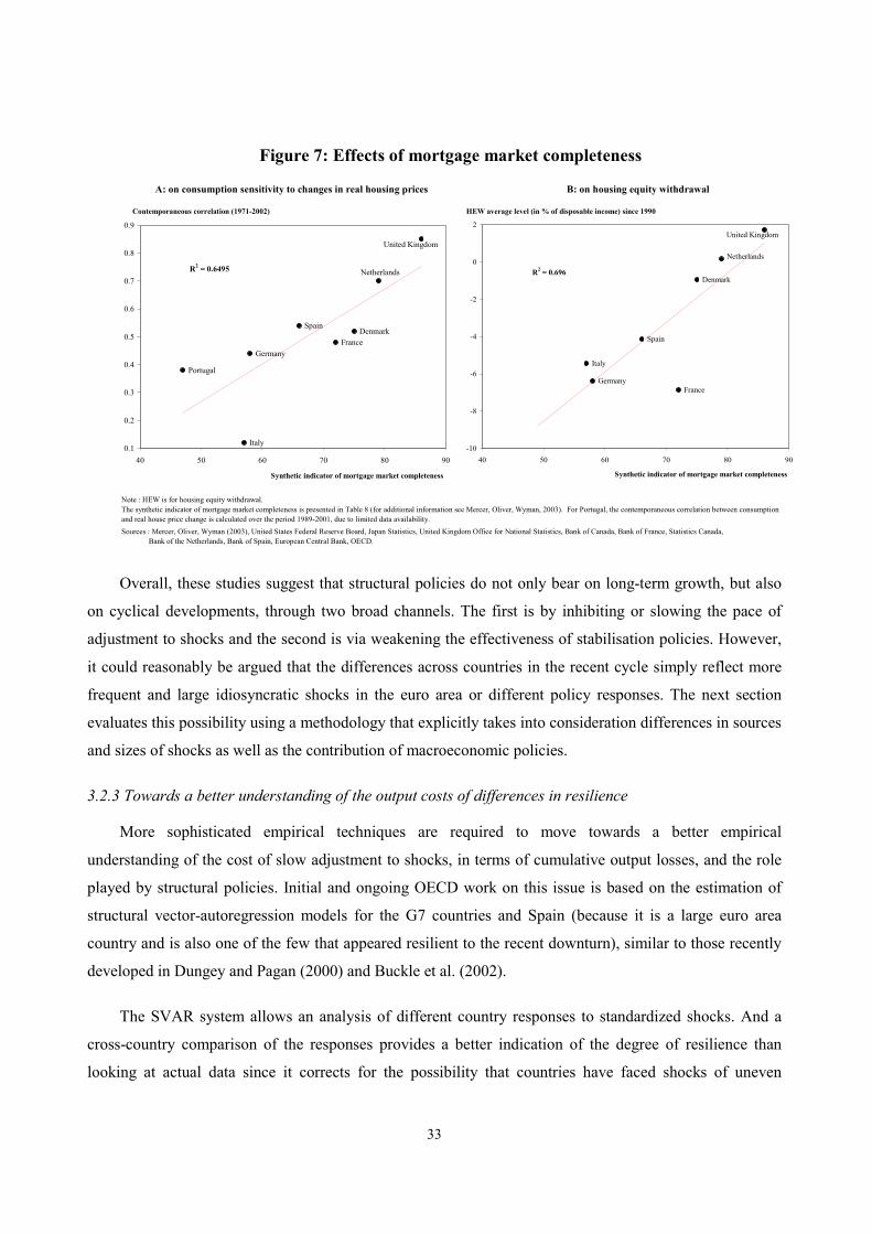
Figure 7: Effects of mortgage market completeness

Note : HEW is for housing equity withdrawal.The synthetic indicator of mortgage market completeness is presented in Table 8 (for additional information see Mercer, Oliver, Wyman, 2003). For Portugal, the contemporaneous correlation between consumptionand real house price change is calculated over the period 1989-2001, due to limited data availability.Sources : Mercer, Oliver, Wyman (2003), United States Federal Reserve Board, Japan Statistics, United Kingdom Office for National Statistics, Bank of Canada, Bank of France, Statistics Canada, Bank of the Netherlands, Bank of Spain, European Central Bank, OECD.

A: on consumption sensitivity to changes in real housing prices B: on housing equity withdrawal

Contemporaneous correlation (1971-2002)

DenmarkFrance

Germany

Italy

Netherlands

Spain

United Kingdom

Portugal

R2 = 0.6495

0.1

0.2

0.3

0.4

0.5

0.6

0.7

0.8

0.9

40 50 60 70 80 90

Synthetic indicator of mortgage market completeness

HEW average level (in % of disposable income) since 1990

United Kingdom

Spain

Netherlands

Italy

GermanyFrance

DenmarkR2 = 0.696

-10

-8

-6

-4

-2

0

2

40 50 60 70 80 90

Synthetic indicator of mortgage market completeness

Overall, these studies suggest that structural policies do not only bear on long-term growth, but also

on cyclical developments, through two broad channels. The first is by inhibiting or slowing the pace of

adjustment to shocks and the second is via weakening the effectiveness of stabilisation policies. However,

it could reasonably be argued that the differences across countries in the recent cycle simply reflect more

frequent and large idiosyncratic shocks in the euro area or different policy responses. The next section

evaluates this possibility using a methodology that explicitly takes into consideration differences in sources

and sizes of shocks as well as the contribution of macroeconomic policies.

3.2.3 Towards a better understanding of the output costs of differences in resilience

More sophisticated empirical techniques are required to move towards a better empirical

understanding of the cost of slow adjustment to shocks, in terms of cumulative output losses, and the role

played by structural policies. Initial and ongoing OECD work on this issue is based on the estimation of

structural vector-autoregression models for the G7 countries and Spain (because it is a large euro area

country and is also one of the few that appeared resilient to the recent downturn), similar to those recently

developed in Dungey and Pagan (2000) and Buckle et al. (2002).

The SVAR system allows an analysis of different country responses to standardized shocks. And a

cross-country comparison of the responses provides a better indication of the degree of resilience than

looking at actual data since it corrects for the possibility that countries have faced shocks of uneven

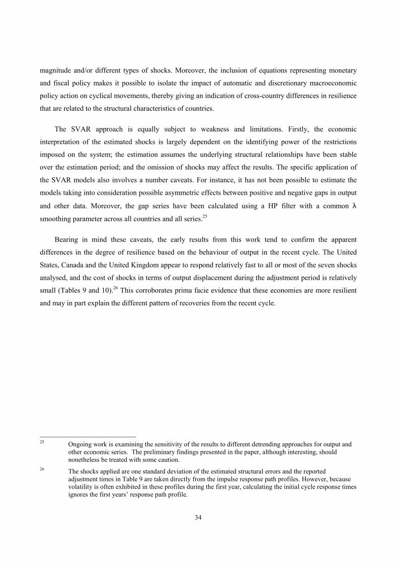
34

magnitude and/or different types of shocks. Moreover, the inclusion of equations representing monetary

and fiscal policy makes it possible to isolate the impact of automatic and discretionary macroeconomic

policy action on cyclical movements, thereby giving an indication of cross-country differences in resilience

that are related to the structural characteristics of countries.

The SVAR approach is equally subject to weakness and limitations. Firstly, the economic

interpretation of the estimated shocks is largely dependent on the identifying power of the restrictions

imposed on the system; the estimation assumes the underlying structural relationships have been stable

over the estimation period; and the omission of shocks may affect the results. The specific application of

the SVAR models also involves a number caveats. For instance, it has not been possible to estimate the

models taking into consideration possible asymmetric effects between positive and negative gaps in output

and other data. Moreover, the gap series have been calculated using a HP filter with a common λ

smoothing parameter across all countries and all series.25

Bearing in mind these caveats, the early results from this work tend to confirm the apparent

differences in the degree of resilience based on the behaviour of output in the recent cycle. The United

States, Canada and the United Kingdom appear to respond relatively fast to all or most of the seven shocks

analysed, and the cost of shocks in terms of output displacement during the adjustment period is relatively

small (Tables 9 and 10).26 This corroborates prima facie evidence that these economies are more resilient

and may in part explain the different pattern of recoveries from the recent cycle.

25 Ongoing work is examining the sensitivity of the results to different detrending approaches for output and

other economic series. The preliminary findings presented in the paper, although interesting, should nonetheless be treated with some caution.

26 The shocks applied are one standard deviation of the estimated structural errors and the reported adjustment times in Table 9 are taken directly from the impulse response path profiles. However, because volatility is often exhibited in these profiles during the first year, calculating the initial cycle response times ignores the first years’ response path profile.

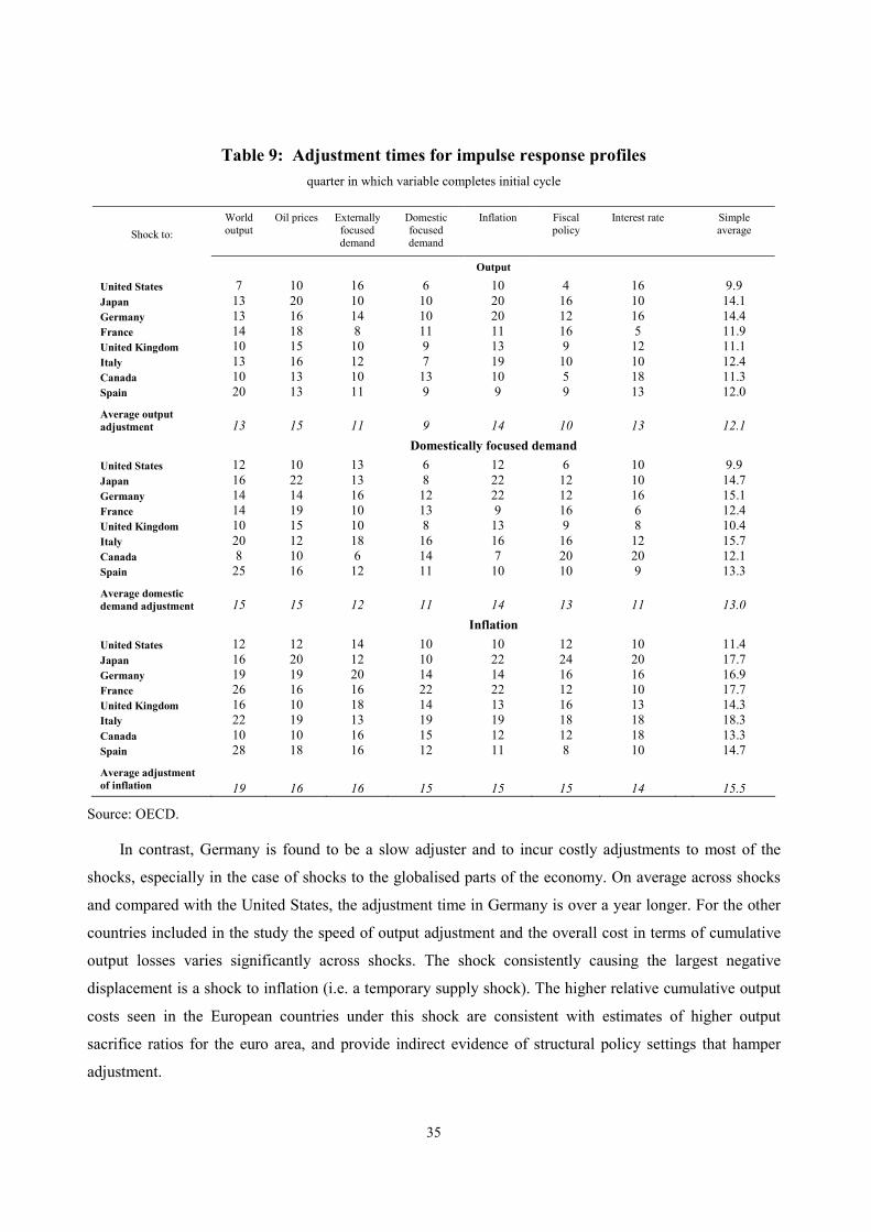
35

Table 9: Adjustment times for impulse response profiles quarter in which variable completes initial cycle

Shock to:

World output

Oil prices Externally focused demand

Domestic focused demand

Inflation Fiscal policy

Interest rate Simple average

Output

United States 7 10 16 6 10 4 16 9.9 Japan 13 20 10 10 20 16 10 14.1 Germany 13 16 14 10 20 12 16 14.4 France 14 18 8 11 11 16 5 11.9 United Kingdom 10 15 10 9 13 9 12 11.1 Italy 13 16 12 7 19 10 10 12.4 Canada 10 13 10 13 10 5 18 11.3 Spain 20 13 11 9 9 9 13 12.0

Average output adjustment 13 15 11 9 14 10 13 12.1

Domestically focused demand United States 12 10 13 6 12 6 10 9.9 Japan 16 22 13 8 22 12 10 14.7 Germany 14 14 16 12 22 12 16 15.1 France 14 19 10 13 9 16 6 12.4 United Kingdom 10 15 10 8 13 9 8 10.4 Italy 20 12 18 16 16 16 12 15.7 Canada 8 10 6 14 7 20 20 12.1 Spain 25 16 12 11 10 10 9 13.3

Average domestic demand adjustment 15 15 12 11 14 13 11 13.0

Inflation United States 12 12 14 10 10 12 10 11.4 Japan 16 20 12 10 22 24 20 17.7 Germany 19 19 20 14 14 16 16 16.9 France 26 16 16 22 22 12 10 17.7 United Kingdom 16 10 18 14 13 16 13 14.3 Italy 22 19 13 19 19 18 18 18.3 Canada 10 10 16 15 12 12 18 13.3 Spain 28 18 16 12 11 8 10 14.7

Average adjustment of inflation 19 16 16 15 15 15 14 15.5

Source: OECD.

In contrast, Germany is found to be a slow adjuster and to incur costly adjustments to most of the

shocks, especially in the case of shocks to the globalised parts of the economy. On average across shocks

and compared with the United States, the adjustment time in Germany is over a year longer. For the other

countries included in the study the speed of output adjustment and the overall cost in terms of cumulative

output losses varies significantly across shocks. The shock consistently causing the largest negative

displacement is a shock to inflation (i.e. a temporary supply shock). The higher relative cumulative output

costs seen in the European countries under this shock are consistent with estimates of higher output

sacrifice ratios for the euro area, and provide indirect evidence of structural policy settings that hamper

adjustment.

36

Table 10: Adjustment costs for output Ratio of cumulative gap of output responses to cumulative gap of variables shocked

World output

Oil prices

Externally focused demand

Domestically focused demand

Inflation Interest rate

Fiscal policy

Simple average absolute

value

Average ex-policy

shocks

United States 0.25 -0.01 0.20 0.11 -0.09 -0.83 0.04 0.22 0.13 Japan 0.25 -0.02 0.28 0.99 -0.44 0.06 -0.55 0.37 0.40 Germany 0.59 -0.05 0.93 0.58 -0.48 -0.69 -1.29 0.66 0.53 France 0.62 -0.03 0.27 0.56 -0.35 -0.02 0.11 0.28 0.37 United Kingdom 0.12 -0.03 0.14 0.20 -0.38 -0.63 0.02 0.22 0.17 Italy 0.20 -0.01 0.16 0.25 -0.33 -0.22 -0.04 0.17 0.19 Canada 0.33 -0.04 0.43 0.36 -0.24 -0.25 0.06 0.24 0.28 Spain 0.54 -0.01 0.23 0.41 -0.27 -0.10 -0.12 0.24 0.29 Average values 0.34 -0.02 0.34 0.44 -0.33 -0.37 -0.24 0.30 0.29

Source: OECD

The SVAR models were also utilized to decompose movements in output gaps in the past into their

main driving forces.27 The rationale for doing this is to assess whether relative lack of resilience in the

larger euro area economies, particularly Germany, suggested by the SVAR results is structural in nature, or

whether it can be explained by ‘bad luck’ (i.e. larger negative shocks to these economies and or less

favourable macroeconomic policy setting). The model analysis confirms that the response of monetary and

fiscal policies has played an important role in buffering the negative shock in the United States in the most

recent period. However, even after purging the impact of macroeconomic policy and shocks to the

globalised parts of the economy, the growth profile in the big continental European countries over the

recent business cycle still seems more sluggish, suggesting intrinsic differences in resilience.

4. Implications for stabilisation policies

The evolving nature of the business cycle bears on the capacity of stabilisation policy to smooth price

and output volatility. Specifically, closer international integration limits the effectiveness of active fiscal

policy, as a result of leakages through trade and other channels of linkage. In the context of a currency

union, however, cycle convergence is necessary for effective monetary policy, and indeed is one of the

criteria for evaluating the suitability of joining a single currency zone.

Even though this study did not find strong support, so far, for closer synchronisation among the 12

OECD countries considered, it is plausible that in the future ongoing globalisation trends will increase

cycle convergence. And it may do so through new channels, such as closer financial market linkages and

27 See Drew et al (forthcoming) for details on the methodology adopted to do this. While such

decompositions can provide valuable information about business cycle dynamics they are dependent on the underlying, highly simplified model. In practice economies are subject to a myriad of economic forces, some of which may be idiosyncratic to a country or a specific time period.

37

asset markets whose prices tend to be determined in global rather than national or local markets.

Accordingly, policy makers need to remain abreast of new business cycle developments.

Forces acting to change international linkages may also bear on the nature of business cycle dynamics

within a country. It is evident, for example, that asset markets now play a bigger role in national

economies. This provides both a source of resilience and a risk to stability. A larger value of traditionally

less liquid assets in balance sheets (i.e. housing) together with flexible and innovative financial markets has

arguably made housing markets more responsive to changes in monetary policy through wealth and

balance sheet effects. This, of course, means that the magnitude of monetary policy responses needed to

modify demand is now smaller than before and it may also have changed the lags in policy transmission in

uncertain ways. These effects need to be better understood.

There is also a danger that the credit and asset price channels of monetary policy transmission have

created new potential sources of price and output instability, because asset prices are prone to substantial

and prolonged periods of misalignments. Indeed, many of the deepest recessions experienced in OECD

countries in the last two decades have been associated with asset price cycles. Obviously, therefore,

misalignments in asset prices should be avoided, but it is less obvious how to do it. Here the conventional

wisdom that monetary policy responds to the extent that asset price developments bear on demand

pressures and thus broader price developments remains, in our view, appropriate. As well, stronger

monitoring of systemic risks and flanking policies that bolster prudential regulation and supervision,

without harming competition and innovation have an expanded role to play. This is happening.

More generally, lack of resilience bears on the cost of output deviations from trend and increases the

risk of hysteresis and the permanent output losses associated with it. Avoiding sharp and persistent falls in

output is therefore of great importance in terms of welfare. Here broader economic policies can help.

Removing market rigidities in product and labour markets raises the adaptability of economies to shocks

and ultimately economies’ potential rate of growth.

Conclusions

This paper has examined two interrelated aspects of business cycles. The first focused on the features

of business cycles within 12 OECD countries, the degree of international synchronisation and how it is

evolving over time. Overall, we find evidence that the severity of cycles has diminished over the past 35

years, reflecting in part improved inventory management techniques, the rising relative importance of

services in overall output and more effective monetary policy frameworks for absorbing nominal shocks.

Regarding the similarity of cyclical characteristics and the strength of their association across countries, the

38

paper examines a number of aspects, including the timing of growth cycle turning points, the length of time

cycles are in a similar phase with the United States and the similarity of cycles with respect to the intensity

of output co-movement. These measures suggest that business cycle synchronisation is high for the 12

OECD countries included in this study, but concerning the evolution of cycle synchronisation through time

the paper is more agnostic. While there appears to be a trend towards increased convergence, this seems at

least partially linked to the reduced severity of cycles in individual countries.

These findings are standard and generally supported in the literature. Yet, they don’t clearly reveal the

recent dichotomy in economic performance between the large euro area economies, which have

experienced a protracted period of excess capacity, and other OECD countries that were better able to

absorb the global shock that prompted the slowdown in 2001. The second part of this paper focused more

closely on this episode, paying particular attention to the interaction between economic policies and the

business cycle. The paper tentatively argues that it is not merely coincidence that the strong performing

OECD economies over the past cycle were also those that undertook ambitious and comprehensive

economic policy reforms over the past 20 years. Nor is it sheer ‘good luck’ in the sense of smaller negative

shocks to these economies and or more favourable macroeconomic policy settings. Rather, recent and

ongoing OECD studies based on panel data regressions and SVAR analysis discussed in this paper bolster

the presumption that flexible product, labour and financial markets not only stimulate potential growth, but

also interact positively with macroeconomic policies to ensure price and output stability. The sense of

disappointment experienced in continental Europe may thus stem as much from the persistence of long-

standing difficulties as from the realisation that other countries have succeeded in turning their economies

around over the years.

Finally, the paper identifies a number of challenges to policy makers that stem from the evolving

features of business cycles within and across countries. Closer international synchronisation will reduce the

effectiveness of active fiscal policy, while the expansion of financial markets increases the potency and

possibly changes the speed of monetary policy transmission through wealth and balance sheet effects.

Policymakers need to better understand the magnitude of these effects. Through the same channels there is

equally a risk of greater price and output instability as a result of misalignments in asset prices. The

conventional wisdom of how to respond to asset price misalignments remains in our opinion appropriate,

though financial supervision institutions must continue to evolve to take account of financial innovation.

Finally, economic policy more generally needs to tackle the lack of resilience to adverse shocks,

particularly in the large euro area countries, by removing micro rigidities in labour and product markets.

39

REFERENCES ARTIS, M., R. BLADEN-HOWELL and W. ZHANG (1995), ‘Turning points in the international business

cycle: an analysis of the OECD leading indicators for the G7 countries’, OECD Economic Studies, No. 24.

BAXTER, M and R. KING (1999), ‘Measuring business cycles: approximate band-pass filters for economic time series’, The Review of Economics and Statistics, Vol. 81, No. 4.

BENJAMIN, J., P. CHINLOY and G. JUD (2003), ‘Real estate versus financial wealth in consumption’, Journal of Real estate Finance and Economics, Vol. 29, No. 3.

BERGOEING, R., P. KEHOE., T. KEHOE, and R. SOTO (2002), ‘A decade lost and found: Mexico and Chile in the 1980s’, Review of Economic Dynamics, Vol. 5.

BERTOLA, G., F. BLAU and L. KAHN (2001), ‘Comparative analysis of labour market outcomes: lessons for the United States from international long-run evidence’, in A.B Krueger and R. Solow, (eds.), The Roaring Nineties: Can Full Employment be Sustained? New York: Russel Sage Foundation.

BLANCHARD, O and D. QUAH (1989), ‘The dynamic effect of aggregate demand and supply disturbances’, American Economic Review, Vol. 79, No.4.

BLANCHARD, O and J. WOLFERS (2000), ‘The role of shocks and institutions in the rise of European unemployment: the aggregate evidence’, Economic Journal, Vol. 110.

BOEHM, E. and W. LIEW (1994), ‘A review of Australia’s recent business cycle experiences and a forecast length of the current expansion’, Australian Economic Review, No. 107.

BUCKLE, R., KUNHONG., H. KIRKHAM., N. McLELLAN and J. SHARMA (2002), ‘A structural VAR model of the New Zealand Business Cycle’, New Zealand Treasury Working Paper, 02/26.

BURNS, A. and W. MITCHELL (1946), Measuring Business Cycles, NBER, New York.

BRY, G. and C. BOSCHAN (1971), Cyclical analysis of time series: selected procedures and computer programs, NBER, New York.

CABALLERO, R and M. HAMMOUR (2000), ‘Creative destruction and development: institutions, crises and restructuring’, World Bank Conference on Development Economics 2000, Washington DC.

CANOVA, F. (1998), ‘Detrending and business cycle facts’, Journal of Monetary Economics, Vol. 41, No. 3.

CASE, E., J. QUIGLEY and R. SHILLER (2001), ‘Comparing wealth effects: the stock market versus the housing market’, NBER Working Paper No. 8606.

CATTE, P., N. GIROUARD, R. PRICE and C. ANDRÉ (2004), ‘Housing markets, wealth and the business cycle’, OECD Economics Department Working Papers, No. 394.

CLAUS, I., P. CONWAY and A. SCOTT (2000), ‘The output gap: measurement, comparisons and assessment’, RBNZ Research Paper, No. 44.

40

COTIS, J.P., J. ELMESKOV and A. MOUROUGANE (2004), ‘Estimates of potential output: benefits and pitfalls from a policy perspective’, in L. Reichlin (ed.) The Euro Area Business Cycle: Stylized Facts and Measurement Issues, CEPR, London.

COTIS, J.P. (2004), ‘Recent developments in macroeconomic analysis: reviving the case for stabilisation policies’, Economie Internationale, No.100.

COURNEDE, B., A. JANOVSKAIA and P, Van den NOORD (2005), ‘Sources of inflation persistence in the euro area’, Paper presented at the XVII Villa Mondragone International Economic Seminar, Rome, 6-7 July.

DALSGAARD, T., J. ELMESKOV and C. PARK (2002), ‘Ongoing changes in the business cycle: evidence and causes’, OECD Economics Department Working Papers, No. 315.

DAVIS, S., J. HALTIWANGER and S. SCHUH (1996), Job Creation and Destruction, Cambridge, Mass. MIT Press.

DEUTSCHE BUNDESBANK (2003), ‘Macroeconomic aspects of share price developments’, Monthly Report, March.

DREW, A., M. KENNEDY and T. SLØK (2004), ‘Differences in resilience between the euro-area and US economies’, OECD Economics Department Working Papers, No. 382.

DUNGEY, M and A. PAGAN (2000), ‘A structural VAR model of the Australian economy’, The Economic Record, Vol. 76.

DVORNAK, N and M. KOHLER (2003), ‘Housing wealth, stock market wealth and consumption: a panel analysis for Australia’, Reserve Bank of Australia, Research Discussion Paper, No. 07, July.

FITOUSSI, J.P, D. JESTAZ., E. PHELPS and G. ZOEGA (2000), ‘Roots of the recent recoveries: labour reforms or private sector forces? Brookings Papers on Economic Activity 1. 2000.

HARDING, D. and A. PAGAN (2001), ‘Extracting, analysing and using cyclical information’, paper Presented at CEPR/Banca d’Italia conference on Monitoring the European Business Cycle, July.

HARDING, D. and A. PAGAN (2002), ‘Dissecting the cycle: a methodological investigation’, Journal of Monetary Economics, Vol. 49, No. 2.

HARDING, D. (2003), ‘Towards an econometric foundation for turning point based analysis of dynamic processes’, Paper presented at the 2003 Australasian Meeting of the Econometric Society.

HARVEY, A. and T. TRIMBUR (2001), ‘General model-based filters for extracting cycles and trends in economic time series’, Cambridge Working Papers in Economics, No. 0113.

HARVEY, A and A. JAEGER (1993), ‘Detrending, stylized facts and the business cycle’, Journal of Applied Econometrics, Vol. 8.

HOELLER, P., C. GIORNO and C. de la MAISONNEUVE (2004), ‘One money, one cycle? Making monetary union a smoother ride’, OECD Economics Department Working Papers, No. 401.

KING, R. and S. REBELLO (1993), ‘Low frequency filtering and real business cycles’, Journal of Economic Dynamics and Control, Vol. 17, No. 1-2.

41

KOSE, A. and K. YI (2002), ‘Can the standard international business cycle model explain the relation between trade and comovement?’, Federal Reserve Bank of Philadelphia Working Paper, No .05-03.

LAXTON, D. and R. TETLOW (1992), ‘A simple multivariate filter for the measurement of potential output’, Bank of Canada Technical Report, No. 59.

LUDWIG, A and T. SLOK (2004), ‘The relationship between stock prices, house prices and consumption in OECD countries’, Topics in Macroeconomics, Vol. 4, Issue 1.

McDERMOTT and A. SCOTT (2000), ‘Concordance in business cycles’, IMF Working Paper, No. 00/37.

MERCER OLIVER WYMAN (2003), Study on the Financial Integration of European Mortgage Markets, European Mortgage Federation, Brussels, October.

OECD (1994), OECD Jobs Study, Evidence and Explanations, Part I: Labour Market Trends and Underlying Forces of Change, Paris.

OECD (2003a), The Sources of Growth in OECD Countries, Paris.

OECD (2003b), Economic Survey of the United Kingdom, Paris.

OSBORN, D.R (1995), ‘Moving average detrending and the analysis of business cycles’, Oxford Bulletin of Economics and Statistics, Vol. 57.

PICHETTE, L and D. TREMBLAY (2003), ‘Are wealth effects important for Canada’, Bank of Canada Working Paper, No. 30, Ottawa, October.

ROMER, C. and D. ROMER (2003), ‘The evolution of economic understanding and postwar stabilization policy perspective’, in Rethinking Stabilization Policy, Jackson Hole Symposium papers, Wyoming, August 29-31, 2002, Federal Reserve Bank of Kansas City.

STOCK, J. and M. WATSON (2004), ‘Has the business cycle changed?’ in Monetary Policy and Uncertainty: Adapting to a Changing Economy, Jackson Hole Symposium papers, Wyoming, August 28-30, 2003, Federal Reserve Bank of Kansas City.

QUAH, D. (1992), ‘The relative importance of permanent and transitory components: identification and some theoretical bounds’, Econometrica, Vol. 60.

Van den NOORD, P. (2004), ‘Modelling cyclical divergences in the euro area: the housing channel’, OECD Economics Department Working Papers, No. 400.

42

Annex 1: Chronology of growth business cycles

Duration (quarters)

Amplitude (% points)

Quarterly amplitude (%

points)

Duration (quarters)

Amplitude (% points)

Quarterly amplitude (%

points)1973Q2 - 1975Q2 8 -6.78 -0.85 1975Q2 - 1979Q2 16 6.20 0.391979Q2 - 1980Q3 5 -3.25 -0.65 1980Q3 - 1981Q2 3 1.28 0.431981Q2 - 1982Q3 13 -5.18 -0.40 1982Q3 - 1984Q3 5 5.43 1.091984Q3 - 1987Q1 9 -1.74 -0.19 1987Q1 - 1989Q4 13 2.23 0.171989Q4 - 1991Q3 7 -3.50 -0.50 1991Q3 - 1994Q3 12 2.36 0.201994Q3 - 1995Q4 5 -1.53 -0.31 1995Q4 - 2000Q2 18 2.96 0.16

Duration (quarters)

Amplitude (% points)

Quarterly amplitude (%

points)

Duration (quarters)

Amplitude (% points)

Quarterly amplitude (%

points)1970Q2 - 1971Q3 3 -4.18 -1.39 1971Q3 - 1973Q2 10 5.60 0.561973Q2 - 1974Q4 9 -6.67 -0.74 1974Q4 - 1979Q3 16 3.34 0.211979Q3 - 1983Q4 6 -2.96 -0.49 1983Q4 - 1985Q3 18 1.69 0.091985Q3 - 1987Q1 4 -2.12 -0.53 1987Q1 - 1990Q4 17 4.35 0.261990Q4 - 1994Q1 11 -3.96 -0.36 1994Q1 - 1997Q1 14 3.67 0.261997Q1 - 1999Q3 6 -3.39 -0.56 1999Q3 - 2000Q4 8 2.80 0.35

Duration (quarters)

Amplitude (% points)

Quarterly amplitude (%

points)

Duration (quarters)

Amplitude (% points)

Quarterly amplitude (%

points)1970Q4 - 1971Q4 4 -1.77 -0.44 1971Q4 - 1973Q3 7 2.72 0.391973Q3 - 1975Q2 7 -5.46 -0.78 1975Q2 - 1979Q4 18 5.70 0.321979Q4 - 1982Q4 12 -4.81 -0.40 1982Q4 - 1986Q1 13 2.30 0.181986Q1 - 1987Q3 6 -1.53 -0.26 1987Q3 - 1991Q1 14 3.83 0.271991Q1 - 1993Q3 10 -3.82 -0.38 1993Q3 - 1995Q1 6 1.82 0.301995Q1 - 1999Q1 16 -1.47 -0.09 1999Q1 - 2000Q3 6 2.48 0.41

Duration (quarters)

Amplitude (% points)

Quarterly amplitude (%

points)

Duration (quarters)

Amplitude (% points)

Quarterly amplitude (%

points)1974Q1 - 1975Q3 6 -4.37 -0.73 1975Q3 - 1979Q4 17 3.30 0.191979Q4 - 1981Q1 5 -2.17 -0.43 1981Q1 - 1982Q2 5 1.39 0.281982Q2 - 1987Q2 20 -1.77 -0.09 1987Q2 - 1990Q1 11 3.04 0.281990Q1 - 1991Q2 5 -1.28 -0.26 1991Q2 - 1992Q1 3 0.68 0.231992Q1 - 1993Q3 6 -2.67 -0.44 1993Q3 - 1995Q1 6 1.78 0.301995Q1 - 1997Q1 8 -1.81 -0.23 1997Q1 - 2000Q4 15 3.20 0.21

Duration (quarters)

Amplitude (% points)

Quarterly amplitude (%

points)

Duration (quarters)

Amplitude (% points)

Quarterly amplitude (%

points)1970Q3 - 1972Q4 9 -3.59 -0.40 1972Q4 - 1974Q1 5 6.46 1.291974Q1 - 1975Q3 6 -7.83 -1.31 1975Q3 - 1976Q4 5 4.80 0.961976Q4 - 1977Q4 4 -3.23 -0.81 1977Q4 - 1980Q2 10 4.32 0.431980Q2 - 1983Q1 11 -4.61 -0.42 1983Q1 - 1985Q3 10 2.04 0.201985Q3 - 1987Q1 6 -0.72 -0.12 1987Q1 - 1990Q1 12 2.11 0.181990Q1 - 1991Q1 4 -1.26 -0.31 1991Q1 - 1992Q1 4 1.13 0.281992Q1 - 1993Q3 6 -3.22 -0.54 1993Q3 - 1995Q4 9 2.68 0.301995Q4 - 1996Q4 4 -1.75 -0.44 1996Q4 - 1997Q4 4 1.55 0.391997Q4 - 1999Q1 5 -1.59 -0.32 1999Q1 - 2001Q1 8 2.26 0.28

Duration (quarters)

Amplitude (% points)

Quarterly amplitude (%

points)

Duration (quarters)

Amplitude (% points)

Quarterly amplitude (%

points)1973Q2 - 1975Q4 10 -6.59 -0.66 1975Q4 - 1979Q3 15 5.52 0.371979Q3 - 1981Q2 7 -5.70 -0.81 1981Q2 - 1983Q4 10 2.82 0.281983Q4 - 1984Q4 4 -1.15 -0.29 1984Q4 - 1988Q3 15 3.16 0.211988Q3 - 1992Q4 17 -4.41 -0.26 1992Q4 - 1994Q4 17 2.75 0.161994Q4 - 1999Q1 17 -0.95 -0.06 1999Q1 - 2000Q3 6 1.29 0.22

Source: OECD Economic Outlook 77 database and OECD calculations.

United States

1970-2003

Downturns (upturn to downturn) Upturns (downturn to upturn)

Period Period

Period Period

Period Period

Italy Downturns (upturn to downturn) Upturns (downturn to upturn)

Japan Downturns (upturn to downturn) Upturns (downturn to upturn)

Period Period

United Kingdom

France Downturns (upturn to downturn) Upturns (downturn to upturn)

Period Period

Downturns (upturn to downturn) Upturns (downturn to upturn)

Downturns (upturn to downturn) Upturns (downturn to upturn)

Period Period

Germany

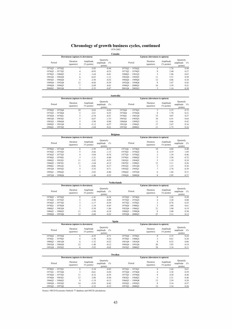
43

Chronology of growth business cycles, continued

Duration (quarters)

Amplitude (% points)

Quarterly amplitude (%

points)

Duration (quarters)

Amplitude (% points)

Quarterly amplitude (%

points)1973Q3 - 1975Q2 7 -3.05 -0.44 1975Q2 - 1976Q2 4 1.76 0.441976Q2 - 1977Q2 4 -0.93 -0.23 1977Q2 - 1979Q3 9 2.40 0.271979Q3 - 1980Q3 4 -1.64 -0.41 1980Q3 - 1981Q2 3 1.88 0.631981Q2 - 1982Q4 6 -6.63 -1.11 1982Q4 - 1985Q3 11 5.51 0.501985Q3 - 1986Q4 5 -2.58 -0.52 1986Q4 - 1989Q4 12 4.06 0.341989Q4 - 1992Q4 12 -4.68 -0.39 1992Q4 - 1994Q4 8 3.47 0.431994Q4 - 1996Q3 7 -2.88 -0.41 1996Q3 - 2000Q3 16 3.39 0.212000Q3 - 2001Q4 5 -2.35 -0.47 2001Q4 - 2002Q3 3 1.14 0.38

Duration (quarters)

Amplitude (% points)

Quarterly amplitude (%

points)

Duration (quarters)

Amplitude (% points)

Quarterly amplitude (%

points)1970Q2 - 1972Q4 10 -2.62 -0.26 1972Q4 - 1973Q3 3 2.15 0.721973Q3 - 1974Q4 5 -2.61 -0.52 1974Q4 - 1976Q4 8 1.70 0.211976Q4 - 1978Q1 5 -2.54 -0.51 1978Q1 - 1981Q4 15 4.07 0.271981Q4 - 1983Q1 5 -6.67 -1.33 1983Q1 - 1985Q3 10 6.41 0.641985Q3 - 1986Q4 5 -3.98 -0.80 1986Q4 - 1989Q3 11 4.66 0.421989Q3 - 1991Q4 9 -5.12 -0.57 1991Q4 - 1996Q1 17 2.67 0.161996Q1 - 1997Q2 5 -1.04 -0.21 1997Q2 - 2000Q1 11 1.73 0.16

Duration (quarters)

Amplitude (% points)

Quarterly amplitude (%

points)

Duration (quarters)

Amplitude (% points)

Quarterly amplitude (%

points)1970Q2 - 1971Q4 6 -1.95 -0.33 1971Q4 - 1974Q2 10 4.04 0.401974Q2 - 1975Q3 5 -5.66 -1.13 1975Q3 - 1976Q3 4 4.19 1.051976Q3 - 1977Q3 4 -3.04 -0.76 1977Q3 - 1978Q2 3 1.39 0.461978Q2 - 1979Q1 3 -1.21 -0.40 1979Q1 - 1980Q2 5 3.58 0.721980Q2 - 1983Q1 11 -3.82 -0.35 1983Q1 - 1984Q2 5 1.19 0.241984Q2 - 1987Q1 11 -1.64 -0.15 1987Q1 - 1990Q1 12 3.11 0.261990Q1 - 1991Q1 5 -0.86 -0.17 1991Q1 - 1991Q4 3 1.13 0.381991Q4 - 1993Q2 5 -3.55 -0.71 1993Q2 - 1995Q1 7 2.70 0.391995Q1 - 1996Q2 5 -2.02 -0.40 1996Q2 - 1997Q4 6 1.84 0.311997Q4 - 1998Q4 4 -1.40 -0.35 1998Q4 - 2000Q4 8 2.95 0.37

Duration (quarters)

Amplitude (% points)

Quarterly amplitude (%

points)

Duration (quarters)

Amplitude (% points)

Quarterly amplitude (%

points)1970Q2 - 1972Q2 8 -1.41 -0.18 1972Q2 - 1974Q2 8 2.24 0.281974Q2 - 1975Q3 5 -3.98 -0.80 1975Q3 - 1976Q3 4 3.20 0.801976Q3 - 1977Q2 3 -1.17 -0.39 1977Q2 - 1978Q1 3 0.76 0.251978Q1 - 1978Q4 3 -1.34 -0.45 1978Q4 - 1980Q1 5 3.04 0.611980Q1 - 1982Q4 3 -5.58 -1.86 1982Q4 - 1986Q1 21 3.90 0.191986Q1 - 1988Q3 11 -1.98 -0.18 1988Q3 - 1990Q4 8 2.40 0.301990Q4 - 1993Q4 12 -2.60 -0.22 1993Q4 - 2000Q3 27 3.11 0.12

Duration (quarters)

Amplitude (% points)

Quarterly amplitude (%

points)

Duration (quarters)

Amplitude (% points)

Quarterly amplitude (%

points)1974Q2 - 1975Q4 6 -4.25 -0.71 1975Q4 - 1978Q1 9 2.15 0.241978Q1 - 1979Q3 6 -1.58 -0.26 1979Q3 - 1980Q2 3 0.61 0.201980Q2 - 1981Q4 6 -1.32 -0.22 1981Q4 - 1983Q4 8 0.52 0.061983Q4 - 1986Q4 12 -1.40 -0.12 1986Q4 - 1991Q4 20 3.83 0.191991Q4 - 1993Q2 6 -3.92 -0.65 1993Q2 - 2000Q2 28 3.14 0.11

Duration (quarters)

Amplitude (% points)

Quarterly amplitude (%

points)

Duration (quarters)

Amplitude (% points)

Quarterly amplitude (%

points)1970Q3 - 1972Q1 6 -5.10 -0.85 1972Q1 - 1973Q1 4 2.44 0.611973Q1 - 1973Q4 3 -0.61 -0.20 1973Q4 - 1974Q4 4 2.38 0.591974Q4 - 1977Q3 11 -4.32 -0.39 1977Q3 - 1979Q4 9 4.30 0.481979Q4 - 1983Q1 13 -3.88 -0.30 1983Q1 - 1984Q2 5 2.31 0.461984Q2 - 1986Q3 9 -1.19 -0.13 1986Q3 - 1989Q4 13 2.59 0.201989Q4 - 1993Q2 14 -5.95 -0.42 1993Q2 - 1995Q3 9 5.14 0.571995Q3 - 1997Q2 7 -2.32 -0.33 1997Q2 - 2000Q2 12 3.14 0.26

Source: OECD Economic Outlook 77 database and OECD calculations.

1970-2003

Period Period

Sweden Downturns (upturn to downturn) Upturns (downturn to upturn)

Downturns (upturn to downturn) Upturns (downturn to upturn)

Period Period

Period Period

Netherlands

Downturns (upturn to downturn) Upturns (downturn to upturn)

Downturns (upturn to downturn) Upturns (downturn to upturn)

Period Period

Spain

Belgium

Canada Downturns (upturn to downturn) Upturns (downturn to upturn)

Period Period

Australia Downturns (upturn to downturn) Upturns (downturn to upturn)

PeriodPeriod

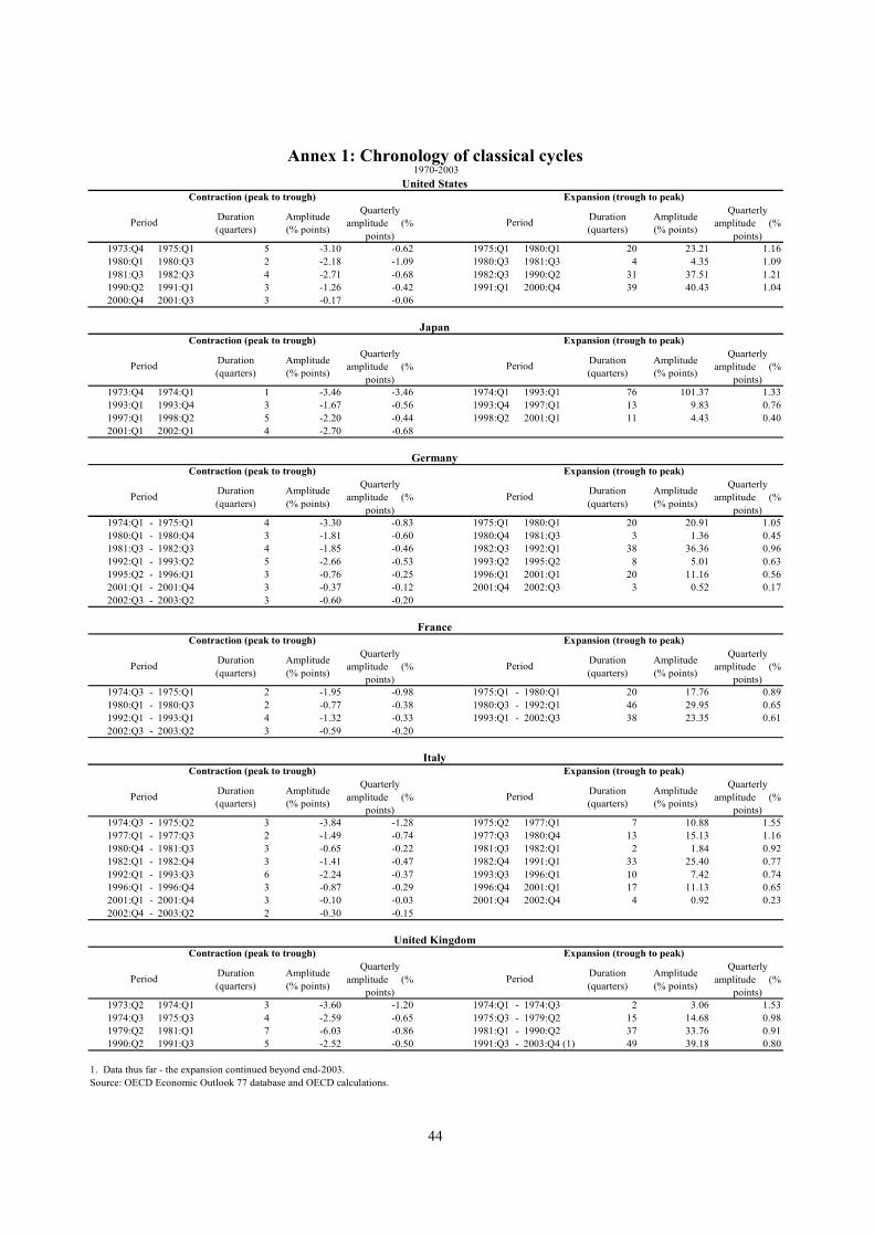
44

Annex 1: Chronology of classical cycles

Duration (quarters)

Amplitude (% points)

Quarterly amplitude (%

points)

Duration (quarters)

Amplitude (% points)

Quarterly amplitude (%

points)1973:Q4 1975:Q1 5 -3.10 -0.62 1975:Q1 1980:Q1 20 23.21 1.161980:Q1 1980:Q3 2 -2.18 -1.09 1980:Q3 1981:Q3 4 4.35 1.091981:Q3 1982:Q3 4 -2.71 -0.68 1982:Q3 1990:Q2 31 37.51 1.211990:Q2 1991:Q1 3 -1.26 -0.42 1991:Q1 2000:Q4 39 40.43 1.042000:Q4 2001:Q3 3 -0.17 -0.06

Duration (quarters)

Amplitude (% points)

Quarterly amplitude (%

points)

Duration (quarters)

Amplitude (% points)

Quarterly amplitude (%

points)1973:Q4 1974:Q1 1 -3.46 -3.46 1974:Q1 1993:Q1 76 101.37 1.331993:Q1 1993:Q4 3 -1.67 -0.56 1993:Q4 1997:Q1 13 9.83 0.761997:Q1 1998:Q2 5 -2.20 -0.44 1998:Q2 2001:Q1 11 4.43 0.402001:Q1 2002:Q1 4 -2.70 -0.68

Duration (quarters)

Amplitude (% points)

Quarterly amplitude (%

points)

Duration (quarters)

Amplitude (% points)

Quarterly amplitude (%

points)1974:Q1 - 1975:Q1 4 -3.30 -0.83 1975:Q1 1980:Q1 20 20.91 1.051980:Q1 - 1980:Q4 3 -1.81 -0.60 1980:Q4 1981:Q3 3 1.36 0.451981:Q3 - 1982:Q3 4 -1.85 -0.46 1982:Q3 1992:Q1 38 36.36 0.961992:Q1 - 1993:Q2 5 -2.66 -0.53 1993:Q2 1995:Q2 8 5.01 0.631995:Q2 - 1996:Q1 3 -0.76 -0.25 1996:Q1 2001:Q1 20 11.16 0.562001:Q1 - 2001:Q4 3 -0.37 -0.12 2001:Q4 2002:Q3 3 0.52 0.172002:Q3 - 2003:Q2 3 -0.60 -0.20

Duration (quarters)

Amplitude (% points)

Quarterly amplitude (%

points)

Duration (quarters)

Amplitude (% points)

Quarterly amplitude (%

points)1974:Q3 - 1975:Q1 2 -1.95 -0.98 1975:Q1 - 1980:Q1 20 17.76 0.891980:Q1 - 1980:Q3 2 -0.77 -0.38 1980:Q3 - 1992:Q1 46 29.95 0.651992:Q1 - 1993:Q1 4 -1.32 -0.33 1993:Q1 - 2002:Q3 38 23.35 0.612002:Q3 - 2003:Q2 3 -0.59 -0.20

Duration (quarters)

Amplitude (% points)

Quarterly amplitude (%

points)

Duration (quarters)

Amplitude (% points)

Quarterly amplitude (%

points)1974:Q3 - 1975:Q2 3 -3.84 -1.28 1975:Q2 1977:Q1 7 10.88 1.551977:Q1 - 1977:Q3 2 -1.49 -0.74 1977:Q3 1980:Q4 13 15.13 1.161980:Q4 - 1981:Q3 3 -0.65 -0.22 1981:Q3 1982:Q1 2 1.84 0.921982:Q1 - 1982:Q4 3 -1.41 -0.47 1982:Q4 1991:Q1 33 25.40 0.771992:Q1 - 1993:Q3 6 -2.24 -0.37 1993:Q3 1996:Q1 10 7.42 0.741996:Q1 - 1996:Q4 3 -0.87 -0.29 1996:Q4 2001:Q1 17 11.13 0.652001:Q1 - 2001:Q4 3 -0.10 -0.03 2001:Q4 2002:Q4 4 0.92 0.232002:Q4 - 2003:Q2 2 -0.30 -0.15

Duration (quarters)

Amplitude (% points)

Quarterly amplitude (%

points)

Duration (quarters)

Amplitude (% points)

Quarterly amplitude (%

points)1973:Q2 1974:Q1 3 -3.60 -1.20 1974:Q1 - 1974:Q3 2 3.06 1.531974:Q3 1975:Q3 4 -2.59 -0.65 1975:Q3 - 1979:Q2 15 14.68 0.981979:Q2 1981:Q1 7 -6.03 -0.86 1981:Q1 - 1990:Q2 37 33.76 0.911990:Q2 1991:Q3 5 -2.52 -0.50 1991:Q3 - 2003:Q4 (1) 49 39.18 0.80

1. Data thus far - the expansion continued beyond end-2003.Source: OECD Economic Outlook 77 database and OECD calculations.

Period Period

United States Contraction (peak to trough) Expansion (trough to peak)

Period Period

Contraction (peak to trough) Expansion (trough to peak)

Period Period

Period Period

Italy

Japan

Contraction (peak to trough) Expansion (trough to peak)

France

Germany

Contraction (peak to trough) Expansion (trough to peak)

Contraction (peak to trough) Expansion (trough to peak)

Period Period

Contraction (peak to trough) Expansion (trough to peak)

Period Period

United Kingdom

1970-2003

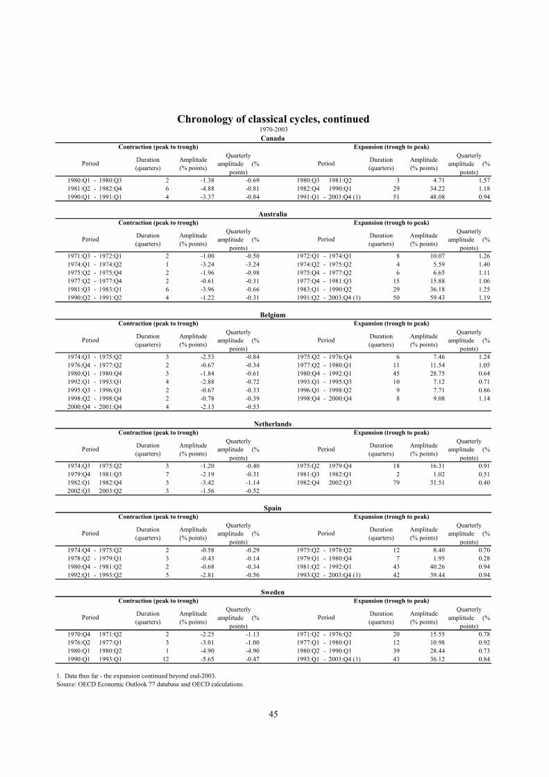
45

Chronology of classical cycles, continued

Duration (quarters)

Amplitude (% points)

Quarterly amplitude (%

points)

Duration (quarters)

Amplitude (% points)

Quarterly amplitude (%

points)1980:Q1 - 1980:Q3 2 -1.38 -0.69 1980:Q3 1981:Q2 3 4.71 1.571981:Q2 - 1982:Q4 6 -4.88 -0.81 1982:Q4 1990:Q1 29 34.22 1.181990:Q1 - 1991:Q1 4 -3.37 -0.84 1991:Q1 - 2003:Q4 (1) 51 48.08 0.94

Duration (quarters)

Amplitude (% points)

Quarterly amplitude (%

points)

Duration (quarters)

Amplitude (% points)

Quarterly amplitude (%

points)1971:Q3 - 1972:Q1 2 -1.00 -0.50 1972:Q1 - 1974:Q1 8 10.07 1.261974:Q1 - 1974:Q2 1 -3.24 -3.24 1974:Q2 - 1975:Q2 4 5.59 1.401975:Q2 - 1975:Q4 2 -1.96 -0.98 1975:Q4 - 1977:Q2 6 6.65 1.111977:Q2 - 1977:Q4 2 -0.61 -0.31 1977:Q4 - 1981:Q3 15 15.88 1.061981:Q3 - 1983:Q1 6 -3.96 -0.66 1983:Q1 - 1990:Q2 29 36.18 1.251990:Q2 - 1991:Q2 4 -1.22 -0.31 1991:Q2 - 2003:Q4 (1) 50 59.43 1.19

Duration (quarters)

Amplitude (% points)

Quarterly amplitude (%

points)

Duration (quarters)

Amplitude (% points)

Quarterly amplitude (%

points)1974:Q3 - 1975:Q2 3 -2.53 -0.84 1975:Q2 - 1976:Q4 6 7.46 1.241976:Q4 - 1977:Q2 2 -0.67 -0.34 1977:Q2 - 1980:Q1 11 11.54 1.051980:Q1 - 1980:Q4 3 -1.84 -0.61 1980:Q4 - 1992:Q1 45 28.75 0.641992:Q1 - 1993:Q1 4 -2.88 -0.72 1993:Q1 - 1995:Q3 10 7.12 0.711995:Q3 - 1996:Q1 2 -0.67 -0.33 1996:Q1 - 1998:Q2 9 7.71 0.861998:Q2 - 1998:Q4 2 -0.78 -0.39 1998:Q4 - 2000:Q4 8 9.08 1.142000:Q4 - 2001:Q4 4 -2.13 -0.53

Duration (quarters)

Amplitude (% points)

Quarterly amplitude (%

points)

Duration (quarters)

Amplitude (% points)

Quarterly amplitude (%

points)1974:Q3 1975:Q2 3 -1.20 -0.40 1975:Q2 1979:Q4 18 16.31 0.911979:Q4 1981:Q3 7 -2.19 -0.31 1981:Q3 1982:Q1 2 1.02 0.511982:Q1 1982:Q4 3 -3.42 -1.14 1982:Q4 2002:Q3 79 31.51 0.402002:Q3 2003:Q2 3 -1.56 -0.52

Duration (quarters)

Amplitude (% points)

Quarterly amplitude (%

points)

Duration (quarters)

Amplitude (% points)

Quarterly amplitude (%

points)1974:Q4 - 1975:Q2 2 -0.58 -0.29 1975:Q2 - 1978:Q2 12 8.40 0.701978:Q2 - 1979:Q1 3 -0.43 -0.14 1979:Q1 - 1980:Q4 7 1.95 0.281980:Q4 - 1981:Q2 2 -0.68 -0.34 1981:Q2 - 1992:Q1 43 40.26 0.941992:Q1 - 1993:Q2 5 -2.81 -0.56 1993:Q2 - 2003:Q4 (1) 42 39.44 0.94

Duration (quarters)

Amplitude (% points)

Quarterly amplitude (%

points)

Duration (quarters)

Amplitude (% points)

Quarterly amplitude (%

points)1970:Q4 1971:Q2 2 -2.25 -1.13 1971:Q2 - 1976:Q2 20 15.55 0.781976:Q2 1977:Q1 3 -3.01 -1.00 1977:Q1 - 1980:Q1 12 10.98 0.921980:Q1 1980:Q2 1 -4.90 -4.90 1980:Q2 - 1990:Q1 39 28.44 0.731990:Q1 1993:Q1 12 -5.65 -0.47 1993:Q1 - 2003:Q4 (1) 43 36.12 0.84

1. Data thus far - the expansion continued beyond end-2003.Source: OECD Economic Outlook 77 database and OECD calculations.

Contraction (peak to trough) Expansion (trough to peak)

Contraction (peak to trough) Expansion (trough to peak)

Period Period

Netherlands

Period Period

Sweden

Contraction (peak to trough) Expansion (trough to peak)

Period Period

Spain

Contraction (peak to trough) Expansion (trough to peak)

Period Period

Expansion (trough to peak)

Period Period

Australia

1970-2003

Period Period

Belgium

Canada

Contraction (peak to trough) Expansion (trough to peak)

Contraction (peak to trough)