Business Cycle Analysis and VARMA Models

Christian Kascha a,∗, Karel Mertens b

aNorges Bank, Research DepartmentbCornell University, Economics Department

Abstract

Can long-run identified structural vector autoregressions (SVARs) discriminate be-tween competing models in practice? Several authors have suggested SVARs failpartly because they are finite-order approximations to infinite-order processes. Weestimate vector autoregressive moving average (VARMA) and state space models,which are not misspecified, using simulated data and compare true with estimatedimpulse responses of hours worked to a technology shock. We find few gains fromusing VARMA models. However, state space algorithms can outperform SVARs. Inparticular, the CCA subspace method consistently yields lower mean squared er-rors, although even these estimates remain too imprecise for reliable inference. Thequalitative differences for algorithms based on different representations are small.The comparison with estimation methods without specification error suggests thatthe main problem is not one of working with a VAR approximation. The propertiesof the processes used in the literature make identification via long-run restrictionsdifficult for any method.

Key words: Structural VARs, VARMA, State Space Models, Business CyclesJEL E32, C15, C52

1 Introduction

This paper compares structural estimation methods based on different reducedform representations of the same economic model in a simulation study sim-ilar to those undertaken by Chari, Kehoe and McGrattan (2005, 2007) and

∗ Corresponding author. Norges Bank, Bankplassen 2, P.O. Box 1179 Sentrum,0107 Oslo, Norway. Tel: +47 22 31 67 19 ; Fax: +47 22 42 40 62.

Email addresses: christian.kascha@norges-bank.no (Christian Kascha),km426@cornell.edu (Karel Mertens).

Preprint submitted to Elsevier June 2008

Christiano, Eichenbaum and Vigfusson (2006). Our aim is to assess differ-ent algorithms’ relative performance and in particular whether the inclusionof moving average terms alone leads to more precise estimates of the struc-tural impulse responses. We focus on the estimation of impact coefficients andlong-run effects of structural shocks. The fact that algorithms based on differ-ent representations yield qualitatively similar results illustrates that the mainproblem with structural identification in this and similar simulation studies isnot one of working within the class of vector autoregressive models.

Structural vector autoregressions are a widely used tool in empirical macroe-conomics, in particular for the evaluation of dynamic stochastic general equi-librium (DSGE) models. Following Sims’s (1989) suggestion, many appliedresearchers have used SVARs to uncover economic relationships without im-posing strong theoretical assumptions. Blanchard and Quah (1989), for ex-ample, use SVARs to discriminate between supply and demand shocks. King,Plosser, Stock and Watson (1991) look at the effects of permanent changes inthe economy on transient economic fluctuations. Christiano and Eichenbaum(1992) investigate the monetary transmission mechanism and Cogley and Na-son (1995) analyze output dynamics in real business cycle (RBC) models. Theresults from SVARs are often viewed as stylized facts that economic mod-els should replicate (see e.g. Christiano and Eichenbaum, 1999). Stock andWatson (2005) provide a useful overview of structural identification methods.

In this literature, a recent discussion has focussed on the impact of technologyshocks on hours worked. In a seminal paper, Gali (1999) identifies productivityinnovations using restrictions on the long-run impact matrix of the structuralerrors. He finds that hours worked fall in response to a positive innovation,which is contrary to the central predictions of the mainstream RBC literature.Many empirical papers have since scrutinized this finding using different datasets and identification schemes. See, for example, the contributions of Chris-tiano, Eichenbaum and Vigfusson (2003); Francis and Ramey (2005a,b) andGali and Rabanal (2005).

In the context of Gali’s (1999) results, there is some debate whether SVARscan in practice discriminate between competing DSGE models and, more gen-erally, whether their sampling properties are good enough to justify their pop-ularity in applied macroeconomics. Chari et al. (2007) and Christiano et al.(2006) investigate the properties of SVARs by simulating artificial data froman RBC model and by comparing true with estimated impulse responses. Inorder to simulate an empirically relevant data generating process (DGP), thestructural parameters of the underlying RBC model are estimated from thedata. According to Chari et al. (2007), long-run identified SVARs fail dramat-ically for both a level and difference specification of hours worked. Even witha correct specification of the integration properties of the series, the SVARoverestimates in most cases the impact of technology on labor and the esti-

2

mates display high variability. However, Christiano et al. (2006) argue thatthe parametrization chosen by Chari et al. (2005, 2007) is not very realistic.With their preferred parametrization, Christiano et al. (2006) find that bothlong-run and short-run identification schemes display only small biases andargue that, on average, the confidence intervals produced by SVARs correctlyreflect the degree of sampling uncertainty. Nevertheless, they also find thatthe estimates obtained via a long-run identification scheme are very impre-cise. These results have been further confirmed by Erceg, Guerrieri and Gust(2005). Kehoe (2006) provides an overview of this debate. On the one hand, itis often difficult to even make a correct inference about the sign of the struc-tural impulse responses with long-run restrictions, and the question is whetherone should use them at all. On the other hand, long-run identification is ap-pealing from a theoretical point of view, since it is usually less model-specificthan short-run identification (Chari et al., 2007). In any case, long-run iden-tification constitutes an additional tool of analysis in applied macroeconomicresearch.

The failure of finite-order SVARs is sometimes attributed to the fact thatthey are only approximations to VARMA / infinite-order VAR processes or tothe possibility that a VAR representation does not exist at all. King, Plosser,and Rebelo (1988) are among the first to recognize that DSGE models im-ply a VARMA representation. Cooley and Dwyer (1998) give an example andstate: “While VARMA models involve additional estimation and identifica-tion issues, these complications do not justify systematically ignoring thesemoving average components, as in the SVAR approach”. As further shownby Fernandez-Villaverde, Rubio-Ramırez, Sargent and Watson (2007), DSGEmodels generally imply a state space system that has a VARMA and eventuallyan infinite VAR representation. Christiano et al. (2006) state that “The spec-ification error involved in using a finite-lag VAR is the reason that in some ofour examples, the sum of VAR coefficients is difficult to estimate accurately”.Most importantly, Chari et al. (2007) argue that a VAR is not able to capturethe underlying VARMA process by showing that the truncation bias, whichis the population bias resulting from applying a finite-order VAR, is the mainsource of the observed small sample bias in their simulation studies. Similarly,Ravenna (2007) shows that applying a finite-order VAR to a DGP generatedby a DSGE model can lead to substantial bias in the structural estimates andstresses that his results do not hinge on small sample bias or on incorrectidentification assumptions. A related time series literature studies estimationand confidence interval construction for impulse responses in VARs in smallsamples (see e.g. Kilian, 2001; Pesavento and Rossi, 2006).

This paper explores the possible advantages of structural VARMA and statespace models that capture the full structure of the time series representationimplied by DSGE models, while imposing minimal theoretical assumptions.We investigate whether estimators based on these alternative representations

3

can outperform SVARs in finite samples. This question is important for sev-eral reasons. First, it is useful to find out to what extent one can improveon SVARs by including moving average components. Second, the question ofwhether estimators based on alternative representations of the same DGP havegood sampling properties is interesting in itself. Employing these alternativesenables researchers to quantify the robustness of their results by comparingdifferent estimates.

In order to assess whether the inclusion of a moving average component leadsto important improvements, we adhere to the research design of Chari et al.(2007) and Christiano et al. (2006): We simulate DSGE models and fit differentreduced form models to recover the structural shocks using the same long-runidentification strategy. As in a closely related study by McGrattan (2006),we then compare the performance of the models by focusing on estimatedcontemporaneous and long-run effects of a productivity shock. We employ avariety of estimation algorithms for the VARMA and state space represen-tations. One of the findings is that one can indeed perform better by takingthe full structure of the DGP into account: While most of the algorithms forVARMA and state space representations do not perform significantly better(and sometimes worse), a subspace algorithm for state space models consis-tently outperforms SVARs in terms of mean squared error. Unfortunately, wealso find that even these alternative estimators are highly variable and arenot necessarily much more informative for discriminating between differentDSGE models. The qualitative differences between the algorithms are smallgiven a particular parametrization of the DSGE model. The emphasis of manyprevious studies on truncation bias suggests that the problems of long-run re-strictions are somewhat specific to the finite-order VAR approximation. Weshow that this is not the case. The bad properties of long-run identificationare not confined to finite-order VARs and, therefore, the main problem withlong-run restrictions in these studies is not one of working within this spe-cific class of models. Instead, we point out some properties of the simulatedDGPs that make it hard to identify structural shocks for any method. Namely,the processes are nearly non-stationary, nearly non-invertible and the correctVARMA representation is close to being not identified.

The rest of the paper is organized as follows. In section 2 we present the RBCmodel used by Chari et al. (2007) and Christiano et al. (2006) that serves asthe basis for our Monte Carlo simulations. In section 3 we discuss the differentstatistical representations of the observed data series. In section 4 we presentthe specification and estimation procedures and the results from the MonteCarlo simulations. Section 5 concludes.

4

2 The Data Generating Process

The DGP for the simulations is based on a simple RBC model taken fromChari et al. (2005, 2007). In the model, a technology shock is the only shockthat affects labor productivity in the long-run, which is the crucial identifyingassumption made by Gali (1999) to assess the role of technology shocks in thebusiness cycle.Households choose infinite sequences, {Ct, Lt, Kt+1 }∞t=0, of per capita con-sumption, labor and capital to maximize expected lifetime utility

E0

∞∑

t=0

[β(1 + γ)]t[log Ct + ψ

(1− Lt)1−σ − 1

1− σ

], (1)

given an initial capital stock K0, and subject to a set of budget constraintsgiven by

Ct + (1 + τx) ((1 + γ)Kt+1 − (1− δ)Kt)≤ (1− τl,t)wtLt + rtKt + Tt, (2)

for t = 0, 1, 2, ..., where wt is the wage, rt is the rental rate of capital, Tt arelump-sum government transfers and τl,t is an exogenous tax on labor income.The parameters include the discount factor β ∈ (0, 1), the labor supply param-eters, ψ > 0 and σ > 0, the depreciation rate δ ∈ (0, 1), the population growthrate γ > 0 and a constant investment tax τx. The production technology is

Yt = Kαt (XtLt)

1−α, (3)

where Xt reflects labor-augmenting technological progress and α ∈ (0, 1) is thecapital income share. Competitive firms maximize Yt − wtLt − rtKt. Finally,the resource constraint is Yt ≥ Ct + (1 + γ)Kt+1 − (1− δ)Kt.The model contains two exogenous shocks, a technology shock and a tax shock,which follow the stochastic processes

log Xt+1 = µ + log Xt + σxεx,t+1, (4a)

τl,t+1 = (1− ρ)τl + ρτl,t + σlεl,t+1, (4b)

where εx,t and εl,t are independent random variables with mean zero and unitstandard deviation and σx > 0 and σl > 0 are scalars. µ > 0 is the mean growthrate of technology, τl > 0 is the mean labor tax and ρ ∈ (0, 1) measures thepersistence of the tax process. Hence, the model has two independent shocks:a unit root process in technology and a stationary AR(1) process in the labortax.

5

3 Statistical Representations

Fernandez-Villaverde et al. (2007) show how the solution of a detrended, log-linearized DSGE model leads to different statistical representations of themodel-generated data. This section presents several alternative ways to writedown a reduced form model for the bivariate, stationary time series

yt =

∆ log(Yt/Lt)

log(Lt)

. (5)

Labor productivity growth, ∆ log(Yt/Lt), and hours worked, log(Lt), are alsothe series analyzed by Gali (1999), as well as Chari et al. (2007) and Chris-tiano et al. (2006). 1 Therefore, the section shows how the structural impulseresponses Gali was interested in are related to different statistical models,given the economic model. The appendix provides more detail on the deriva-tions. Given the log-linearized solution of the RBC model of the previoussection, we can write down the law of motion of the logs

log kt+1 = φ1 + φ11 log kt − φ11 log xt + φ12τl,t, (6a)

log yt − log Lt = φ2 + φ21 log kt − φ21 log xt + φ22τl,t, (6b)

log Lt = φ3 + φ31 log kt − φ31 log xt + φ32τl,t, (6c)

where kt = Kt/Xt+1 and yt = Yt/Xt are capital and output detrended with theunit-root shock and xt = Xt/Xt−1. The φ’s are the coefficients of the calculatedpolicy rules. Following Fernandez-Villaverde et al. (2007), the system can bewritten in state space form. The state transition equation is

log kt+1

τl,t

= K1 + A

log kt

τl,t−1

+ B

εx,t

εl,t

, (7)

xt+1 = K1 + Axt + Bεt,

and the observation equation is

1 There are also different information sets that are equally applicable in the presentcontext, e.g. [∆yt lt]′ which would be more in line with Blanchard et al. (1989). Thisdecision should be based on the statistical properties of the series. Results for thisalternative information set can be found in a web appendix to this paper.

6

∆ log(Yt/Lt)

log Lt

= K2 + C

log kt

τl,t−1

+ D

εx,t

εl,t

, (8)

yt = K2 + Cxt + Dεt,

where K1, A,B, K2, C and D are constant matrices that depend on the co-efficients of the policy rules and therefore on the “deep” parameters of themodel. The state vector is given by xt = [log kt, τl,t−1]

′ and the noise vector isεt = [εx,t, εl,t]

′. Note that the system has a state vector of dimension two withthe logarithm of detrended capital and the tax rate shock as state components.

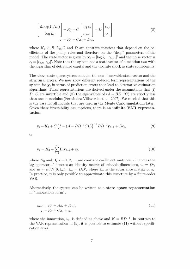
The above state space system contains the non-observable state vector and thestructural errors. We now show different reduced form representations of thesystem for yt in terms of prediction errors that lead to alternative estimationalgorithms. These representations are derived under the assumptions that (i)D, C are invertible and (ii) the eigenvalues of (A− BD−1C) are strictly lessthan one in modulus (Fernandez-Villaverde et al., 2007). We checked that thisis the case for all models that are used in the Monte Carlo simulations later.Given these invertibility assumptions, there is an infinite VAR represen-tation:

yt = K3 + C(I − (A−BD−1C)L

)−1BD−1yt−1 + Dεt, (9)

or

yt = K3 +∞∑

i=1

Πiyt−i + ut, (10)

where K3 and Πi, i = 1, 2, . . . are constant coefficient matrices, L denotes thelag operator, I denotes an identity matrix of suitable dimensions, ut = Dεt

and ut ∼ iid N(0, Σu), Σu = DD′, where Σu is the covariance matrix of ut.In practice, it is only possible to approximate this structure by a finite-orderVAR.

Alternatively, the system can be written as a state space representationin “innovations form”:

xt+1 = K1 + Axt + Kut, (11)

yt = K2 + Cxt + ut,

where the innovation, ut, is defined as above and K = BD−1. In contrast tothe VAR representation in (9), it is possible to estimate (11) without specifi-cation error.

7

Finally, the underlying DGP can be represented by a VARMA(1,1) repre-sentation:

yt = K4 + CAC−1yt−1 +(D + (CB − CAC−1D)L

)εt, (12)

yt = K4 + A1yt−1 + ut + M1ut−1,

where the last equation defines the constant coefficient matrices A1, M1, K4

and ut is defined as above. As with the above state space representation, theVARMA(1,1) representation can also be estimated with no specification error.

Given the conditions stated in Fernandez-Villaverde et al. (2007), all threerepresentations are equivalent. They are just different ways of writing downthe same process. However, the properties of estimators and tests depend onthe chosen statistical representation. It should be emphasized that we arealways interested in the same process and ultimately in the estimation ofthe same coefficients, i.e. those associated with the first-period response ofyt to a unit shock in εx,t to the technology process. However, the differentrepresentations give rise to different estimation algorithms and therefore ourstudy can be regarded as a comparison of different algorithms to estimate thesame linear system.

4 The Monte Carlo Experiment

4.1 Monte Carlo Design and Econometric Techniques

To investigate the properties of the various estimators, we simulate 1000 sam-ples of the vector series yt in linearized form and transform log-deviations tovalues in log-levels. As in the previous Monte Carlo studies, the sample sizeis 180 quarters. We use two different sets of parameter values: The first is dueto Chari et al. (2005, 2007) and is referred to as the CKM specification, whilethe second is the one used by Christiano et al. (2006) and is labeled the KPspecification, referring to estimates obtained by Prescott (1986). 2 The spe-cific parameter values are given in table 1 for the CKM and KP benchmarkspecifications. To check the robustness of our results, we also consider vari-ations of the benchmark models. As in Christiano et al. (2006), we considerdifferent values for the preference parameter σ and the standard deviation ofthe labor tax, σl. These variations change the fraction of the business cycle

2 Both parameterizations are obtained by maximum likelihood estimation of thetheoretical model, using time series on productivity and hours worked in the US.However, because of differences in approach, both papers obtain different estimates.

8

variability that is due to technology shocks. The different values for σ arereported in table 2. For the CKM specification, we also consider cases whereσl assumes a fraction of the original benchmark value. Christiano et al. (2006)show that the key difference between the specifications is the implied fractionof the variability in hours worked that is due to technology shocks.

In the following, we present the long-run identification scheme of Blanchardet al. (1989). Consider the following infinite moving average representation ofyt in terms of ut:

yt =∞∑

i=0

Φu,iut−i = Φu(L)ut, (13)

where we abstract from the intercept term and Φu(L) is a lag polynomial,Φu(L) =

∑∞i=0 Φu,iL

i. Analogously, we can represent yt in terms of the struc-tural errors using the relation ut = Dεt:

yt =∞∑

i=0

Φu,iDεt−i = Φε(L)εt, (14)

where Φε(L) =∑∞

i=0 Φu,iDLi. The former lag polynomial, evaluated at one,

Φu(1) = I + Φu,1 + Φu,2 + . . . (15)

is the long-run impact matrix of the reduced form error ut. Note that theexistence of this infinite sum depends on the stationarity of the series. If thestationarity requirement is violated or “nearly” violated, then the long-runidentification scheme is not valid or may face difficulties. Also note that thematrix D defined in section 3 gives the first-period impact of shocks in εt. Usingthe above relations, we know that Φε(1) = Φu(1)D and further Σu = DD′,where Φε(1) is the long-run impact matrix of the underlying structural errors.The identifying restriction on Φε(1) is that only the technology shock has apermanent effect on labor productivity. This restriction implies that in ourbivariate system the long-run impact matrix is triangular,

Φε(1) =

Φ11 0

Φ21 Φ22

, (16)

and it is assumed that Φ11 > 0. Using Φε(1)Φ′ε(1) = Φu(1)ΣuΦ

′u(1) we can

obtain Φε(1) from the Cholesky decomposition of Φu(1)ΣuΦ′u(1). The contem-

poraneous impact matrix can be recovered from D = [Φu(1)]−1Φε(1). Corre-spondingly, the estimated versions are

9

Φε(1) = chol[Φu(1)ΣuΦ′u(1)], (17a)

D = [Φu(1)]−1Φε(1). (17b)

Only the first column of D is identified and is our estimate of the first-periodimpact of the technology shock. 3

Next, we comment on the estimation techniques. First, note that for eachrepresentation there is more than one reasonable estimation method. We triedseveral algorithms for all representations but chose to present only the resultsfor the algorithms that worked best for each representation. 4 Of course, itis still possible that there are algorithms that work slightly better for one ofthe representations in the current setting. However, the aim of this study isprimarily to quantify whether the inclusion of the moving average term aloneleads to important gains in terms of more precise estimates of the structuralparameters. For all methods described below, we ensure that stationary andinvertible models are obtained.

Vector Autoregressive Models: VARs are well known, so we commentonly on a few issues. As in the previous Monte Carlo studies, the lag lengthis set at four and the VAR is estimated by OLS. However, for different setsof parameter values a VAR with a different number of lags may yield slightlybetter results. We have chosen to stick to the VAR(4) because we want tofacilitate comparison with the results of Christiano et al. (2006) and becausethere was no lag order that performed uniformly better for all DGPs. 5 En-forcing stationarity of the estimated model improves the VAR results to someextent.

State Space Models: There are many ways to estimate a state spacemodel, e.g. maximum likelihood methods based on the Kalman filter or sub-space identification methods such as N4SID of Van Overschee and De Moor(1994) or the CCA method of Larimore (1983). We use the CCA subspace al-gorithm that was previously found to be remarkably accurate in small samples.As argued by Bauer (2005a), CCA might be the best algorithm for economet-ric applications. It is also asymptotically equivalent to maximum likelihood

3 Alternatively, one could solve for D directly using the three restrictions impliedby Σu = DD′ and the long-run identifying restriction (Blanchard et al., 1989), sincethe Cholesky decomposition can occasionally produce an ill conditioned matrix. Inthe present context, however, the results from both strategies are identical.4 Additional results and programs may be obtained from the authors.5 Data dependent criteria such as AIC are unfortunately not very helpful for theseDGPs. Results for the VAR with AIC selection are presented in a web appendix tothis paper. See also Chari et al. (2007).

10

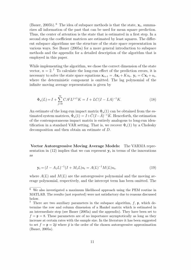
(Bauer, 2005b). 6 The idea of subspace methods is that the state, xt, summa-rizes all information of the past that can be used for mean square prediction.Thus, the center of attention is the state that is estimated in a first step. In asecond step the coefficient matrices are estimated by least squares. The differ-ent subspace algorithms use the structure of the state space representation invarious ways. See Bauer (2005a) for a more general introduction to subspacemethods and the appendix for a detailed description of the algorithm that isemployed in this paper.

While implementing the algorithm, we chose the correct dimension of the statevector, n = 2. 7 To calculate the long-run effect of the prediction errors, it isnecessary to solve the state space equations xt+1 = Axt +Kut, yt = Cxt +ut,where the deterministic component is omitted. The lag polynomial of theinfinite moving average representation is given by

Φu(L) = I +∞∑

j=0

CAjLj+1K = I + LC(I − LA)−1K. (18)

An estimate of the long-run impact matrix Φu(1) can be obtained from the es-timated system matrices, Φu(1) = I+C(I−A)−1K. Henceforth, the estimationof the contemporaneous impact matrix is entirely analogous to long-run iden-tification in a standard VAR setting. That is, we recover Φε(1) by a Choleskydecomposition and then obtain an estimate of D.

Vector Autoregressive Moving Average Models: The VARMA repre-sentation in (12) implies that we can represent yt in terms of the innovationsas

yt = (I − A1L)−1(I + M1L)ut = A(L)−1M(L)ut, (19)

where A(L) and M(L) are the autoregressive polynomial and the moving av-erage polynomial, respectively, and the intercept term has been omitted. The

6 We also investigated a maximum likelihood approach using the PEM routine inMATLAB. The results (not reported) were not satisfactory due to reasons discussedbelow.7 There are two auxiliary parameters in the subspace algorithm, f , p, which de-termine the row and column dimension of a Hankel matrix which is estimated inan intermediate step (see Bauer (2005a) and the appendix). They have been set tof = p = 8. These parameters are of no importance asymptotically as long as theyincrease at certain rates with the sample size. In the literature it has been suggestedto set f = p = 2p where p is the order of the chosen autoregressive approximation(Bauer, 2005a).

11

long-run impact of the innovations can be estimated by Φu(1) = A(1)−1M(1)and an estimate of the first column of D can be obtained as before. Instead ofestimating the VARMA(1,1) representation in (12) we chose a specific repre-sentation which guarantees that all parameters are identified and the numberof moving average parameters is minimal. For an introduction to the identi-fication problem in VARMA models see Lutkepohl (2005). Here we employ afinal moving average (FMA) representation that can be derived analogouslyto the final equation form (see Dufour and Pelletier, 2004). In our case, thisresults in a VARMA (2, 1) representation in final moving average form (seeappendix). 8

As in the case of state space models there are many different estimation meth-ods for VARMA models. Examples are the methods developed by Durbin(1960), Hannan and Rissanen (1982), the generalized least-squares algorithm(Koreisha and Pukkila, 1990), full information maximum likelihood (Mauri-cio, 1997) or Kapetanios’s (2003) iterative least-squares algorithm. We triedthe mentioned algorithms but report results for the best performing methodwhich is a simple two-stage least squares algorithm also known as the Hannan-Rissanen method. The method starts with an initial “long” autoregression inorder to estimate the unobserved residuals. The estimated residuals are thentreated as observed and a (generalized) least squares regression is performed.We use a VAR with lag length nT = 0.5

√T for the initial long autoregres-

sion. 9

4.2 Results of the Monte Carlo Study

Tables 2 - 3 summarize the results of the Monte Carlo simulation study. Ta-ble 2 displays Monte Carlo means and standard deviations of the estimatesof the contemporaneous impact of a technology shock on productivity andhours. That is, the estimates of 100 times the first column of D, 100 ·D[., 1].Likewise, table 3 shows Monte Carlo means and standard deviations of thedifferent structural estimators for the percent long-run effect, 100 ·Φε[., 1]. Wechose to compute means and standard deviations based on a trimmed sampleof estimates for the long-run effects. Trimming of replications associated withthe most extreme upper and lower estimates is beneficial because of a few out-

8 We experimented with other identified representations such as the final equationrepresentation or the Echelon representation. However, the final moving averagerepresentation yielded the best results.9 In particular, we also tried full information maximum likelihood maximization asformulated in Mauricio (1997). However, this procedure proved to be highly unstableand was therefore not considered to be a practical alternative. One reason is thatthe roots of the AR and the MA polynomials are all close to the unit circle.

12

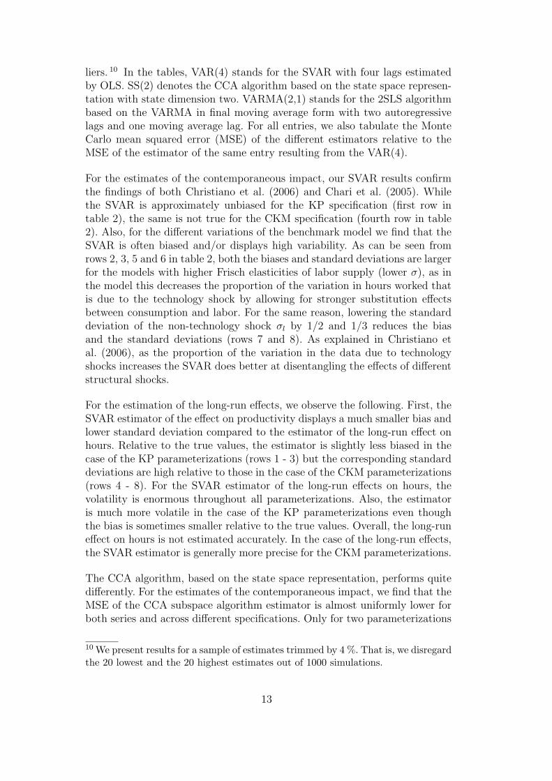
liers. 10 In the tables, VAR(4) stands for the SVAR with four lags estimatedby OLS. SS(2) denotes the CCA algorithm based on the state space represen-tation with state dimension two. VARMA(2,1) stands for the 2SLS algorithmbased on the VARMA in final moving average form with two autoregressivelags and one moving average lag. For all entries, we also tabulate the MonteCarlo mean squared error (MSE) of the different estimators relative to theMSE of the estimator of the same entry resulting from the VAR(4).

For the estimates of the contemporaneous impact, our SVAR results confirmthe findings of both Christiano et al. (2006) and Chari et al. (2005). Whilethe SVAR is approximately unbiased for the KP specification (first row intable 2), the same is not true for the CKM specification (fourth row in table2). Also, for the different variations of the benchmark model we find that theSVAR is often biased and/or displays high variability. As can be seen fromrows 2, 3, 5 and 6 in table 2, both the biases and standard deviations are largerfor the models with higher Frisch elasticities of labor supply (lower σ), as inthe model this decreases the proportion of the variation in hours worked thatis due to the technology shock by allowing for stronger substitution effectsbetween consumption and labor. For the same reason, lowering the standarddeviation of the non-technology shock σl by 1/2 and 1/3 reduces the biasand the standard deviations (rows 7 and 8). As explained in Christiano etal. (2006), as the proportion of the variation in the data due to technologyshocks increases the SVAR does better at disentangling the effects of differentstructural shocks.

For the estimation of the long-run effects, we observe the following. First, theSVAR estimator of the effect on productivity displays a much smaller bias andlower standard deviation compared to the estimator of the long-run effect onhours. Relative to the true values, the estimator is slightly less biased in thecase of the KP parameterizations (rows 1 - 3) but the corresponding standarddeviations are high relative to those in the case of the CKM parameterizations(rows 4 - 8). For the SVAR estimator of the long-run effects on hours, thevolatility is enormous throughout all parameterizations. Also, the estimatoris much more volatile in the case of the KP parameterizations even thoughthe bias is sometimes smaller relative to the true values. Overall, the long-runeffect on hours is not estimated accurately. In the case of the long-run effects,the SVAR estimator is generally more precise for the CKM parameterizations.

The CCA algorithm, based on the state space representation, performs quitedifferently. For the estimates of the contemporaneous impact, we find that theMSE of the CCA subspace algorithm estimator is almost uniformly lower forboth series and across different specifications. Only for two parameterizations

10 We present results for a sample of estimates trimmed by 4 %. That is, we disregardthe 20 lowest and the 20 highest estimates out of 1000 simulations.

13

(fourth and fifth rows) does the MSE of the CCA-based estimates exceedthe MSE of the SVAR, and only by a relatively small amount. In particular,the first-period impact on hours worked is estimated more precisely up to areduction to 87% in terms of MSE for the KP specification. In almost all casesthe bias is at least slightly reduced. Second, although the response of hoursworked is usually estimated more precisely, the performances of the subspacealgorithm and the SVAR are clearly related: in cases where the SVAR doespoorly, the state space model does the same. For example, both algorithmsdo relatively well for the KP parametrization but fail dramatically for theCKM parametrization with indivisible labor. Third, we also note that theCCA algorithm is most advantageous relative to the VAR when the VARis most precise, i.e., for the KP parameterizations. Fourth, even though theCCA algorithm can be more precise, the structural estimators are still highlyvariable and not necessarily much more useful in a qualitative sense.

For the estimates of the long-run effects, the findings are similar. The CCAalgorithm does better than the SVAR for most parameterizations. Notableexceptions are the results for the long-run effect on productivity for two CKMparameterizations (rows four and five). The performances of the CCA algo-rithm and the SVAR are related in the sense that both estimators are moreprecise for the KP parameterizations. The CCA estimator of the long-run ef-fects of a technology shock can be much more precise than the correspondingSVAR estimator. For example, the standard deviation is dramatically reducedin case of the KP parameterizations. Still, even this estimator does not resolvethe essential problem, i.e. the standard deviations are far too large to make areliable qualitative judgement.

The results for the VARMA algorithm are about the same to worse comparedto those for the VAR approximation. In contrast to the CCA algorithm, wedo not observe an improvement from the VARMA-based estimator of the con-temporaneous impact. In most cases, the mean bias of the VARMA estimatorsis higher than the bias resulting from the VAR, while the standard deviationis slightly reduced. Also, the performance of the VARMA algorithm is relatedto the performance of the VAR over different parameterizations of the model.The VARMA yields weaker results in the most difficult cases (rows four andfive). This finding mirrors the results for the CCA algorithm. Although theVARMA model fully nests the underlying DGP, the associated algorithm isnot that efficient in our context.

Again, the results for the long-run effect of a technology shock are similaralthough it seems that the 2SLS algorithm does better in estimating theseeffects than in estimating the contemporaneous impact. Also, the performanceof this estimator is highly positively correlated with the performance of theSVAR estimator. Therefore, as in the case of the CCA algorithm based on thestate space representation, also this estimator is essentially uninformative.

14

We summarize the findings for all three algorithms as follows:

• The precision of the structural estimators differs more over the different pa-rameterizations of the benchmark model than between different estimatorsgiven the same parametrization.

• While the the CCA algorithm appears superior to the VAR in the simula-tions, the performances of all reported algorithms do not differ too much ina qualitative sense given a particular parametrization.

• For all examples considered, the standard deviations of all estimators of thecontemporaneous and long-run effect on hours are quite large, making theestimates uninformative.

These results illustrate clearly that the unresolved question of what is theempirically relevant parametrization or economic model is quite important.From the work of Christiano et al. (2006), it is reasonable to conclude thatthe differences in bias between different parameterizations is mostly due tovariation of the relative importance of technology shocks for the fluctuationsin hours worked. Note, however, that the mean of the estimator is not a goodsummary of its small sample behavior because the variance is so large thatalmost no weight is attached to values close to the mean. In the case of the KPbenchmark parametrization, the effect on hours is estimated with a standarddeviation of 0.43 given a mean of 0.32. Here, a more relevant loss function isthe MSE or some other measure that takes more than the first moment intoaccount. In terms of the MSE, long-run restrictions perform poorly also in thiscase.

Two questions arise: Why do all estimators perform so poorly and why dosimple methods (e.g. VAR vs. VARMA) perform generally better in the sim-ulations? Using the VARMA representation we can point out three problemswith the simulated DGPs. The processes are nearly non-stationary, nearlynon-invertible and the correct VARMA representation is close to being notidentified. Estimators based on the state space or VARMA representation aremore sophisticated and less robust to the near violation of the assumptions onwhich they are built. This disadvantage seems to compensate to some extentfor the advantage of nesting the DSGE model.

We use a general VARMA(p, q) representation for a K-dimensional process topoint out the features of the simulated DGPs:

A(L)yt = M(L)ut,

where the constant has been omitted. A(L) = I − A1L − . . . − LApLp is the

autoregressive and M(L) = I + M1L + . . . + LMqLq is the moving polynomial

with corresponding eigenvalues λari , λma

i , i = 1, 2, . . . which are the inverseroots of det A(z) and det M(z), z ∈ C, respectively. Now, the process is sta-

15

tionary and invertible if and only if all eigenvalues are less than one in modulus(Lutkepohl, 2005). In our case |λar

i | < 1 |λmai | < 1 for i = 1, 2. Table 1 provides

these eigenvalues for the benchmark specifications. For example, for the CKMparametrization these are λar

1 = 0.9573 , λar2 = 0.94, λma

1 = −0.9557 andλma

2 = 0. Note that the moving average part is not of full rank. These valuesare very similar for all other parameterizations. That is, all these processesare nearly non-stationary and non-invertible. 11

The fact that one eigenvalue of the moving average part is very close to oneeigenvalue of the autoregressive part in modulus is again not confined to theCKM parametrization. It is true for all processes. This point suggests thatthe VARMA(1,1) representation, though formally correct, is close to beingnot identified (Klein, Melard and Spreij, 2005). We know that a VARMA rep-resentation is identified if and only if the corresponding Fisher Informationmatrix (FIM) is non-singular. Formally, the FIM is the negative expected sec-ond derivative of the likelihood function with respect to the parameter vector.Klein et al. (2005) prove that the FIM is singular if and only if it is the casethat λar

i = −λmai for at least one i. According to Klein et al. (2005), singularity

of the FIM is equivalent to singularity of the tensor Sylvester matrix set forthby Gohberg and Lerer (1976)

S⊗(−M, A) :=

(−IK)⊗IK (−M1)⊗IK ... (−Mq)⊗IK 0 ... 0

0... ... ...

......

... ... ... ... 00 ... (−IK)⊗IK (−M1)⊗IK ... (−Mq)⊗IK

IK⊗IK IK⊗(−A1) ... IK⊗(−Ap) 0 ... 0

0... ... ...

......

... ... ... 00 ... 0 IK⊗IK IK⊗(−A1) ... IK⊗(−Ap)

,

where 0 denotes here the null matrix of dimension (K2 × K2). Klein et al.(2005) propose checking the singularity of this matrix instead of checking thesingularity of the FIM directly for numerical reasons. For example, for theCKM benchmark the determinant of the tensor Sylvester matrix is 0.000023.We can perturb the process by changing slightly the eigenvalue of the mov-ing average matrix from -0.9557 to -0.9573. The determinant of the tensorSylvester matrix jumps to 0. 12 That is, even though the DSGE model impliesa VARMA(1,1), the process is hard to distinguish from a lower dimensionalprocess. We think that this feature is the most likely explanation why Chari

11 The near non-stationarity has also been noticed by other authors such as Chariet al. (2007).12 Formally, we compute the eigenvalue decomposition M1 = V ΛV −1 and changethe corresponding entry in Λ. The “perturbed” moving average matrix is then M1 =V ΛV −1 and the corresponding process is yt = A1yt−1 + ut + M1ut−1.

16

et al. (2007) find that the usual VAR lag-selection criteria often suggest aVAR(1). 13

It is clear that a potential lack of identification can be a severe problem forthe estimation of the impulse responses in general. In addition, it is well doc-umented that near non-identification is especially problematic for the estima-tion of (vector) ARMA models. See e.g. the introduction in Melard, Roy andSaidi (2006) or Ansley and Newbold (1980) for an early documentation. Itis also known in the literature on VARMA estimation that processes whichare close to being non-invertible are difficult to estimate. Again, Ansley et al.(1980) provide an early account of this problem as well as Davidson (1981)for pure moving-average models. Additionally, the stationarity assumption isat the heart of the long-run identification strategy. While we ensure that theestimated model is stable, the high autoregressive roots will induce small sam-ple bias. These problems are faced by all representations and explain why theobserved poor performance is not specific to the VAR methodology. We alsohesitate to make any strong recommendation in favor of a particular class ofalgorithms because of the special nature of the simulated processes. However,a sensible strategy might be to consider several estimators at the same time,such as a VAR and the CCA method, and to aggregate the results in someway as suggested by a thick modeling approach (Granger and Jeon, 2004).

How do these results relate to other results in the literature? First, we thinkthat our results are broadly confirmed by the studies of McGrattan (2006) andMertens (2007). Mertens (2007) uses spectral methods, proposed by Chris-tiano et al. (2006), to estimate technology shocks in a similar setting. He findsthat methods based on the frequency domain, though correctly specified, dopoorly and concludes that the observed bias is a result of the small sample sizeused. Since two of the algorithms used in this paper nest the DSGE modeland therefore are also correctly specified, one would attribute the errors tothe limited sample size as well. On the other hand, Chari et al. (2005, 2007)and Ravenna (2007) stress that the bias in the SVAR estimates are due to thefinite-order truncation used and not to small sample problems. These differentconclusions are largely due to different terminology, since these authors are re-ferring to the so-called Hurwicz-type small-sample bias (Hurwicz, 1950). Thatis, the difference in mean between a SVAR(4) estimated on a finite sample anda SVAR(4) estimated on an infinite sample. If the lag length is viewed as afunction of the sample size p(T ) when it comes to approximating infinite VARprocesses, then the bias is simply due to T being small. Our study suggests,however, that when the true DGP induces a large truncation bias in the VARestimates, estimation of other representations is equally difficult. For futureresearch, we believe attention should be shifted away from the evaluation of a

13 Unfortunately, estimating a lower-dimensional processes does not yield a uniformimprovement either.

17

particular model class and towards the study of the statistical processes oneis confronted with and, as in Christiano et al. (2006), the question of whetherthe usual bootstrap inference is reliable. Particularly, interesting in this case isthe construction of confidence intervals in cases of highly persistent processesas e.g. in Pesavento and Rossi (2006).

5 Conclusions

There has been some debate whether long-run identified SVARs can in practicediscriminate between competing DSGE models and whether their samplingproperties are good enough to justify their widespread use. Several MonteCarlo studies indicate that SVARs based on long-run restrictions are oftenbiased and usually imprecise. Some authors have suggested that SVARs dopoorly because they are only approximate representations of the underly-ing DGPs. Therefore, we replicate the simulation experiments of Chari etal. (2007) and Christiano et al. (2006) and apply more general models totheir simulated data. In particular, we use algorithms based on VARMA andstate space representations of the data and compare the resulting estimatesof the underlying structural model. For our simulations, we found that onecan do better by taking the full structure of the DGP into account. While ourVARMA-based estimation algorithms and some algorithms for state spacemodels were not found to perform significantly better and often even worse,the CCA subspace algorithm seems to consistently outperform the VAR ap-proximation. However, the estimators display high variability and are oftenbiased, regardless of the reduced form model used. Furthermore, the perfor-mances of the different estimators are strongly correlated. The comparisonwith estimation methods without specification error suggests that the themain problem is not one of working with a VAR approximation insofar asthe properties of the processes used in the literature make identification vialong-run restrictions difficult for any method.

In this study, we assumed that the integration orders of the series as well asthe lag lengths of the true VARMA process are known. Future research couldtherefore be directed towards the effects of various forms of uncertainty aboutthe correct specification and the construction of inference methods which arerobust to various forms of misspecification.

Acknowledgment

We would like to thank Anindya Banerjee, Wouter Denhaan, Helmut Her-wartz, Helmut Lutkepohl, Morten O. Ravn, Pentti Saikkonen and participants

18

at the “Recent Developments in Econometrics” conference in Florence, as wellas seminar participants at the Bank of Spain and Norges Bank for valuablecomments and discussion. The comments and suggestions from two anony-mous referees and the editor have been especially useful for improving theexposition in the paper. The research for this paper was conducted at theEuropean University Institute. The views expressed in this paper are our ownand do not necessarily reflect the views of Norges Bank.

19

Appendix A: Final MA Equation Form

Consider a standard representation for a stationary and invertible VARMA(p, q) process

A(L)yt = M(L)ut.

Recall that M−1(L) = M∗(L)/|M(L)|, where M∗(L) denotes the adjoint ofM(L) and |M(L)| its determinant. We can multiply the above equation withM∗(L) to get

M∗(L)A(L)yt = |M(L)|ut.

This representation therefore places restrictions on the moving average poly-nomial which is required to be a scalar operator, |M(L)|. Dufour et al. (2004)show that this restriction leads to an identified representation. More specif-ically, consider the VARMA(1,1) representation in (12). Since the movingaverage part is not of full rank we can write the system as

1− a11L −a12L

−a21L 1− a22L

yt =

1 + m11L αm11L

m21L 1 + αm21L

ut,

where α is some constant not equal to zero and the intercept is omitted.Clearly, det(M(L)) = 1 + (m11 + αm21)L and therefore

1+αm21L −αm11L

−m21L 1+αm11L

1−a11L −a12L

−a21L 1−a22L

yt=[1+(m11+αm21)L]ut.

Because of the reduced rank we end up with a VARMA (2, 1). Note that themoving average part is indeed restricted to be a scalar operator.

Appendix B: Statistical Representations

This section elaborates on the derivation of the infinite VAR, VARMA andstate space representations that result from our DSGE model in order to get aninsight into the relationship between the economic model and the implied timeseries properties. The derivation follows Fernandez-Villaverde et al. (2007). Analternative way to derive a state space system for the purpose of maximum

20

likelihood estimation can be found in Ireland (2001).Consider again the law of motion of the logs

log kt+1 = φ1 + φ11 log kt − φ11 log xt + φ12τl,t,

log yt − log Lt = φ2 + φ21 log kt − φ21 log xt + φ22τl,t,

log Lt = φ3 + φ31 log kt − φ31 log xt + φ32τl,t,

and the exogenous states

log xt+1 = µ + σxεx,t+1,

τlt+1 = (1− ρ)τl + ρτl,t + σlεl,t+1.

From these equations the state space representation can be derived as follows.First, write down the law of motion of labor productivity in differences:

∆ log(Yt/Lt) = log xt + φ21∆ log kt − φ21∆ log xt + φ22∆τl,t.

Thus the observed series can be expressed as

∆ log(Yt/Lt) = φ21 log kt − φ21 log kt−1 + (1− φ21) log xt

+φ21 log xt−1 + φ22τl,t − φ22τl,t−1,

log Lt = φ3 + φ31 log kt − φ31 log xt + φ32τl,t.

Next, rewrite the law of motion for capital as

log kt−1 = −φ−111 φ1 + φ−1

11 log kt + log xt−1 − φ−111 φ12τl,t−1,

in order to substitute for capital at time t− 1:

∆ log(Yt/Lt) = φ21φ−111 φ1 + φ21(1− φ−1

11 ) log kt

+(1− φ21) log xt + φ22τl,t + (φ21φ−111 φ12 − φ22)τl,t−1.

Using the laws of motion for the stochastic shock processes, substitute thecurrent exogenous shocks to get

21

∆ log(Yt/Lt) =[φ21φ

−111 φ1 + (1− φ21)µ + φ22(1− ρ)τl

]

+φ21(1− φ−111 ) log kt + (φ21φ

−111 φ12 − (1− ρ)φ22)τl,t−1

+(1− φ21)σxεx,t + φ22σlεl,t,

log Lt = [φ3 − φ31µ + φ32(1− ρ)τl] + φ31 log kt + φ32ρτl,t−1

−φ31σxεx,t + φ32σlεl,t.

Next, consider the law of motion for capital and express future capital in termsof the current states as

log kt+1 = [φ1 − φ11µ + φ12(1− ρ)τl] + φ11 log kt + φ12ρτl,t−1

−φ11σxεx,t + φ12σlεl,t.

Collecting the above equations, the system can be written in state space formaccording to Fernandez-Villaverde et al. (2007). The state transition equationis

log kt+1

τl,t

= K1 + A

log kt

τl,t−1

+ B

εx,t

εl,t

,

where the system matrices are given by

K1 =

φ1 − φ11µ + φ12(1− ρ)τl

(1− ρ)τ

, A =

φ11 φ12ρ

0 ρ

and

B =

−φ11σx φ12σl

0 σl

.

The observation equation is

∆ log(Yt/Lt)

log Lt

= K2 + C

log kt

τl,t−1

+ D

εx,t

εl,t

,

22

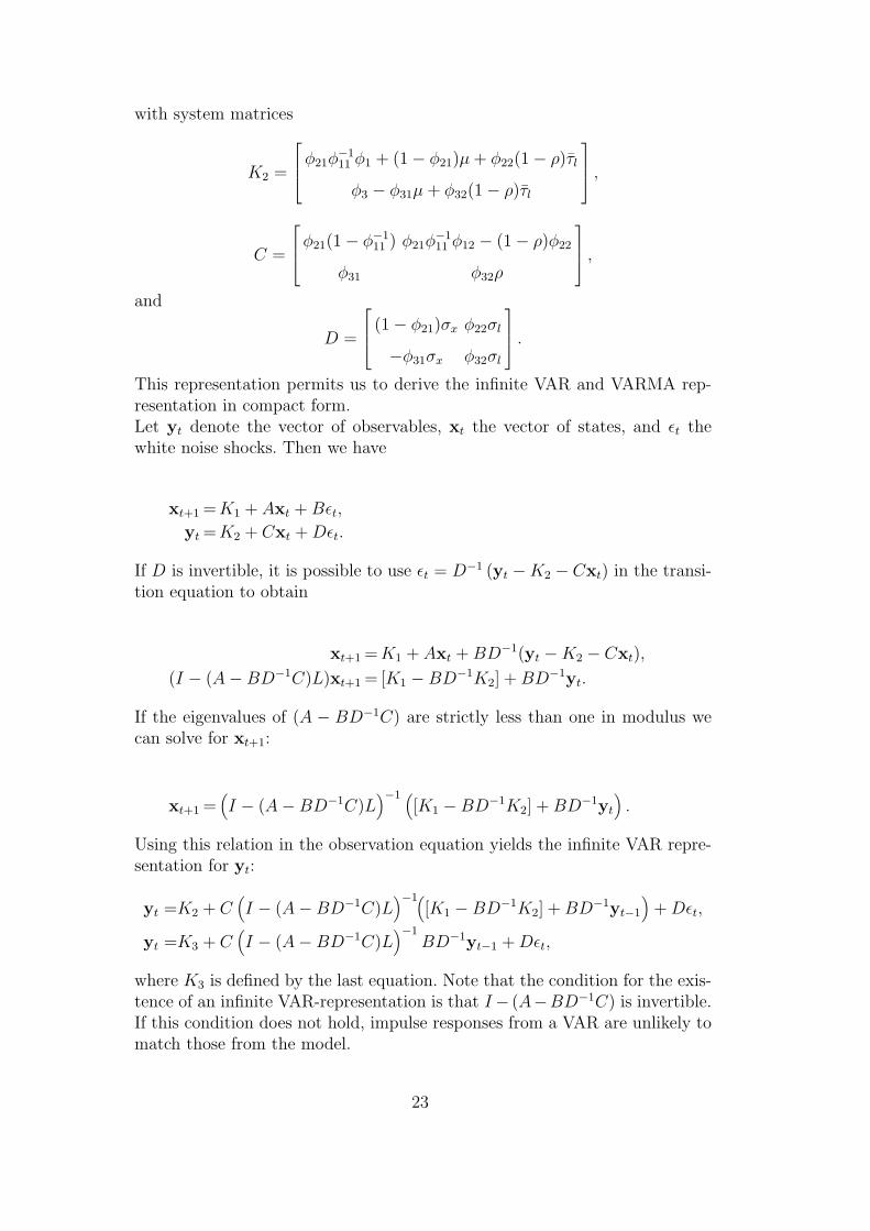
with system matrices

K2 =

φ21φ−111 φ1 + (1− φ21)µ + φ22(1− ρ)τl

φ3 − φ31µ + φ32(1− ρ)τl

,

C =

φ21(1− φ−111 ) φ21φ

−111 φ12 − (1− ρ)φ22

φ31 φ32ρ

,

and

D =

(1− φ21)σx φ22σl

−φ31σx φ32σl

.

This representation permits us to derive the infinite VAR and VARMA rep-resentation in compact form.Let yt denote the vector of observables, xt the vector of states, and εt thewhite noise shocks. Then we have

xt+1 = K1 + Axt + Bεt,

yt = K2 + Cxt + Dεt.

If D is invertible, it is possible to use εt = D−1 (yt −K2 − Cxt) in the transi-tion equation to obtain

xt+1 = K1 + Axt + BD−1(yt −K2 − Cxt),

(I − (A−BD−1C)L)xt+1 = [K1 −BD−1K2] + BD−1yt.

If the eigenvalues of (A − BD−1C) are strictly less than one in modulus wecan solve for xt+1:

xt+1 =(I − (A−BD−1C)L

)−1 ([K1 −BD−1K2] + BD−1yt

).

Using this relation in the observation equation yields the infinite VAR repre-sentation for yt:

yt =K2 + C(I − (A−BD−1C)L

)−1([K1 −BD−1K2] + BD−1yt−1

)+ Dεt,

yt =K3 + C(I − (A−BD−1C)L

)−1BD−1yt−1 + Dεt,

where K3 is defined by the last equation. Note that the condition for the exis-tence of an infinite VAR-representation is that I− (A−BD−1C) is invertible.If this condition does not hold, impulse responses from a VAR are unlikely tomatch those from the model.

23

If C is invertible, it is possible to rewrite the state as

xt = C−1 (yt −K2 −Dεt) ,

and use it in the transition equation:

C−1 (yt+1 −K2 −Dεt+1) = K1 + AC−1 (yt −K2 −Dεt) + Bεt,

yt+1 − CAC−1yt = CK1 + K2 − CAC−1K2

+(CB − CAC−1D)εt + Dεt+1.

Therefore, we obtain a VARMA(1,1) representation of yt:

yt = K4 + CAC−1yt−1 +(I + (CBD−1 − CAC−1)L

)Dεt,

where K4 is defined by the equation.

Appendix C: Estimation Algorithms

Two-Stage Least Squares

This simple estimator uses VAR modeling in a first step to estimate the un-known residuals. In the second step these are used to replace the true inno-vations in the VARMA equations and the coefficient matrices are estimatedby least squares. The procedure is easy to implement and is sometimes calledthe Hannan-Rissanen method or Durbin’s method (Durbin, 1960; Hannan etal., 1982). The resulting estimators are not asymptotically efficient (Hannanand Deistler, 1988, chapter 6). We discuss the method in the framework of astandard VARMA (p, q) representation

yt = A1yt−1 + . . . + Apyt−p + ut + M1ut−1 + . . . + Mqut−q.

Usually, additional restrictions need to be imposed on the coefficient matricesto ensure identification of the parameters.Given that the moving average polynomial is invertible, there exists an infiniteVAR representation of the process, yt =

∑∞i=1 Πiyt−i + ut. In the first step of

both algorithms, this representation is approximated by a “long” VAR to getan estimate of the residuals. More precisely, the following regression equationis used

24

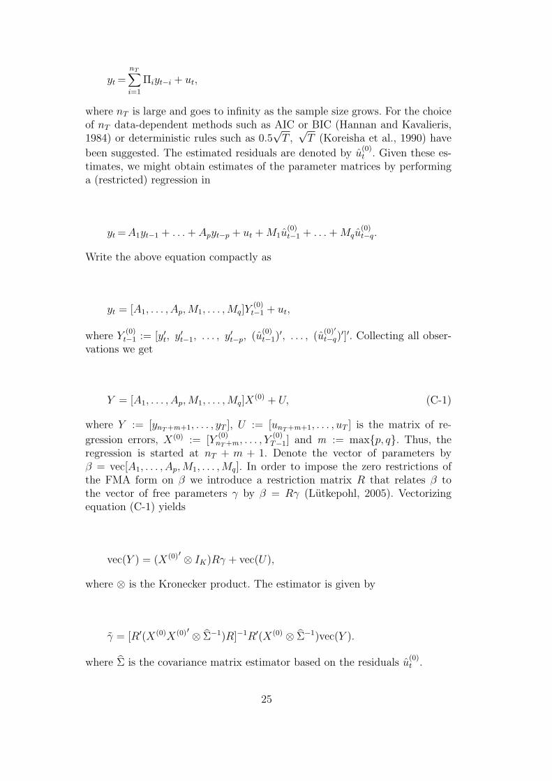
yt =nT∑

i=1

Πiyt−i + ut,

where nT is large and goes to infinity as the sample size grows. For the choiceof nT data-dependent methods such as AIC or BIC (Hannan and Kavalieris,1984) or deterministic rules such as 0.5

√T ,

√T (Koreisha et al., 1990) have

been suggested. The estimated residuals are denoted by u(0)t . Given these es-

timates, we might obtain estimates of the parameter matrices by performinga (restricted) regression in

yt = A1yt−1 + . . . + Apyt−p + ut + M1u(0)t−1 + . . . + Mqu

(0)t−q.

Write the above equation compactly as

yt = [A1, . . . , Ap,M1, . . . ,Mq]Y(0)t−1 + ut,

where Y(0)t−1 := [y′t, y′t−1, . . . , y′t−p, (u

(0)t−1)

′, . . . , (u(0)′t−q)

′]′. Collecting all obser-vations we get

Y = [A1, . . . , Ap,M1, . . . , Mq]X(0) + U, (C-1)

where Y := [ynT +m+1, . . . , yT ], U := [unT +m+1, . . . , uT ] is the matrix of re-

gression errors, X(0) := [Y(0)nT +m , . . . , Y

(0)T−1] and m := max{p, q}. Thus, the

regression is started at nT + m + 1. Denote the vector of parameters byβ = vec[A1, . . . , Ap,M1, . . . , Mq]. In order to impose the zero restrictions ofthe FMA form on β we introduce a restriction matrix R that relates β tothe vector of free parameters γ by β = Rγ (Lutkepohl, 2005). Vectorizingequation (C-1) yields

vec(Y ) = (X(0)′ ⊗ IK)Rγ + vec(U),

where ⊗ is the Kronecker product. The estimator is given by

γ = [R′(X(0)X(0)′ ⊗ Σ−1)R]−1R′(X(0) ⊗ Σ−1)vec(Y ).

where Σ is the covariance matrix estimator based on the residuals u(0)t .

25

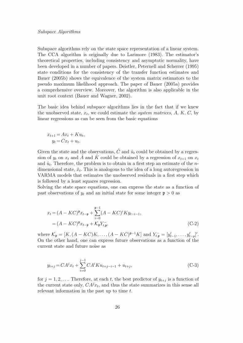
Subspace Algorithms

Subspace algorithms rely on the state space representation of a linear system.The CCA algorithm is originally due to Larimore (1983). The estimator’stheoretical properties, including consistency and asymptotic normality, havebeen developed in a number of papers. Deistler, Peternell and Scherrer (1995)state conditions for the consistency of the transfer function estimates andBauer (2005b) shows the equivalence of the system matrix estimators to thepseudo maximum likelihood approach. The paper of Bauer (2005a) providesa comprehensive overview. Moreover, the algorithm is also applicable in theunit root context (Bauer and Wagner, 2002).

The basic idea behind subspace algorithms lies in the fact that if we knewthe unobserved state, xt, we could estimate the system matrices, A, K, C, bylinear regressions as can be seen from the basic equations

xt+1 = Axt + Kut,

yt = Cxt + ut.

Given the state and the observations, C and ut could be obtained by a regres-sion of yt on xt and A and K could be obtained by a regression of xt+1 on xt

and ut. Therefore, the problem is to obtain in a first step an estimate of the n-dimensional state, xt. This is analogous to the idea of a long autoregression inVARMA models that estimates the unobserved residuals in a first step whichis followed by a least squares regression.Solving the state space equations, one can express the state as a function ofpast observations of yt and an initial state for some integer p > 0 as

xt = (A−KC)pxt−p +p−1∑

i=0

(A−KC)iKyt−i−1,

= (A−KC)pxt−p +KpY−t,p, (C-2)

where Kp = [K, (A −KC)K, . . . , (A −KC)p−1K] and Y −t,p = [y′t−1, . . . , y

′t−p]

′.On the other hand, one can express future observations as a function of thecurrent state and future noise as

yt+j = CAjxt +j−1∑

i=0

CAiKut+j−i−1 + ut+j, (C-3)

for j = 1, 2, . . .. Therefore, at each t, the best predictor of yt+j is a function ofthe current state only, CAjxt, and thus the state summarizes in this sense allrelevant information in the past up to time t.

26

Define Y +t,f = [y′t, . . . , y

′t+f−1]

′ for some integer f > 0 and formulate equation(C-3) for all observations contained in Y +

t,f simultaneously. Combine theseequations with (C-2) in order to obtain

Y +t,f =OfKpY

−t,p +Of (A−KC)pxt−p + EfE

+t,f ,

where Of = [C ′, A′C ′, . . . , (Af−1)′C ′]′, E+t,f = [u′t, . . . , u

′t+f−1]

′ and Ef is a func-tion of the system matrices. The above equation is central for most subspacealgorithms. Note that if the maximum eigenvalue of (A − KC) is less thanone in absolute value, we have (A −KC)p ≈ 0 for large p. This condition issatisfied for stationary and invertible processes. This reasoning motivates anapproximation of the above equation by

Y +t,f = βY −

t,p + N+t,f , (C-4)

where β = OfKp and N+t,f is defined by the equation. Most popular subspace

algorithms use this equation to obtain an estimate of β that is decomposedinto Of and Kp. The identification problem is solved implicitly during thisstep.For given integers, n, p, f , the employed algorithm consists of the followingsteps:

(1) Set up Y +t,f and Y −

t,p and perform OLS in (C-4) using the available data

to get an estimate βf,p.(2) Compute the sample covariances

Γ+f =

1

Tf,p

T−f+1∑

t=p+1

Y +t,f (Y

+t,f )

′ , Γ−p =1

Tf,p

T−f+1∑

t=p+1

Y −t,p(Y

−t,p)

′,

where Tf,p = T − f − p + 1.(3) Given the dimension of the state, n, compute the singular value decom-

position

(Γ+f )−1/2βf,p(Γ

−p )1/2 = UnΣnV

′n + Rn,

where Σn is a diagonal matrix that contains the n largest singular valuesand Un and Vn are the corresponding singular vectors. The remainingsingular values are neglected and the approximation error is Rn. Thereduced rank matrices are obtained as

Of Kp = [(Γ+f )1/2UnΣ1/2

n ][Σ1/2n V ′

n(Γ−p )−1/2].

(4) Estimate the state as xt = KpY−t,p and estimate the system matrices using

linear regressions as described above.

27

Although the algorithm appears complicated, it is simple to implement andis believed to produce a numerically stable and accurate estimator. There arecertain parameters which have to be determined prior to estimation, namelythe dimension of the state and the integers f and p. For the asymptotic con-sequences of various choices see Bauer (2005a).

28

References

Ansley, C.F., Newbold, P., 1980. Finite Sample Properties of Estimators for Au-toregressive Moving Average Models. Journal of Econometrics 13, 159–183.

Bauer, D., 2005a. Estimating Linear Dynamical Systems Using Subspace Methods.Econometric Theory, 21 (1), 181–211.

Bauer, D., 2005b. Comparing the CCA Subspace Method to Pseudo MaximumLikelihood Methods in the Case of no Exogenous Inputs. Journal of Time SeriesAnalysis, 26 (5), 631–668.

Bauer, D., Wagner, M., 2002. Estimating Cointegrated Systems Using SubspaceAlgorithms. Journal of Econometrics, 111, 47–84.

Blanchard, O.J., Quah, D., 1989. The Dynamic Effects of Aggregate Demand andSupply Disturbances. American Economic Review 79 (4), 655–673.

Chari, V.V., Kehoe, P.J. , McGrattan, E.R., 2005. A Critique of Structural VARsUsing Real Business Cycle Theory. Federal Reserve Bank of Minneapolis, WorkingPaper 631.

Chari, V.V., Kehoe, P.J. , McGrattan, E.R., 2007. Are Structural VARs with Long-Run Restrictions Useful in Developing Business Cycle Theory? Federal ReserveBank of Minneapolis, Staff Report 364.

Christiano, L.J., Eichenbaum, M., 1992. Identification and the Liquidity Effect of aMonetary Policy Shock, in: Cukierman, A., Hercowitz, Z., Leiderman, L. (Eds.),Political Economy, Growth and Business Cycles, Cambridge: The MIT Press.

Christiano, L.J., Eichenbaum, M., 1992. The research agenda: Larry Christiano andMartin Eichenbaum write about their current research progam on the monetarytransmission mechanism. Economic Dynamics Newsletter 1(1). Society for Eco-nomic Dynamics, http://www.economicdynamics.org.

Christiano, L.J., Eichenbaum, M., Vigfusson, R., 2003. What Happens After a Tech-nology Shock? NBER working paper 9819.

Christiano, L.J., Eichenbaum, M., Vigfusson, R., 2006. Assessing Structural VARs,in: Acemoglu, D., Rogoff, K. and Woodford, M. (Eds.), NBER MacroeconomicsAnnual 2006, Cambridge: The MIT Press.

Cogley, T., Nason, J.M., 1995. Output Dynamics in Real Business Cycle Models.American Economic Review 85 (3), 492–511.

Cooley, T.F., Dwyer, M., 1998. Business Cycle Analysis Without Much Theory. ALook at Structural VARs. Journal of Econometrics 83 (1-2), 57–88.

Davidson, J.E.H., 1981. Problems with the Estimation of Moving Average Processes.Journal of Econometrics 16, 295–310.

Deistler, M., Peternell, K., Scherrer, W., 1995. Consistency and Relative Efficiencyof Subspace Methods. Automatica 31, 1865–1875.

Dufour, J.-M., Pelletier D., 2002. Linear Estimation of Weak VARMA Models Witha Macroeconomic Application, Universite de Montreal and North Carolina StateUniversity, working paper. Version: March 2004.

Durbin, J., 1960. The Fitting of Time-Series Models. Revue de l’Institut Inter-national de Statistique/Review of the International Statistical Institute 28 (3),233-244.

Erceg, C.J., Guerrieri, L., Gust, C.J., 2005. Can Long-Run Restrictions Identify

29

Technology Shocks? Journal of the European Economic Association 3 (4), 1237–1278.

Fernandez-Villaverde, J., Rubio-Ramırez, J.F., Sargent, T.J., Watson, M.W., 2007.A,B,C’s (and D)’s For Understanding VARs. American Economic Review 97 (3),1021–1026.

Francis, N., Ramey, V. A., 2005. Is the Technology-Driven Real Business Cycle Hy-pothesis Dead? Shocks and Aggregate Fluctuations Revisited. Journal of Mone-tary Economics 52 (8), 1379–99.

Francis, N., Ramey, V. A., 2005. Measures of Per-Capita Hours and Their Implica-tions for the Technology-Hours Debate. NBER working paper 11694.

Gali, J., 1999. Technology, Employment, and the Business Cycle: Do TechnologyShocks Explain Aggregate Fluctuations? American Economic Review 89 (1), 249–271.

Gali, J., Rabanal, P., 2005. Technology Shocks and Aggregate Fluctuations: Howwell does the RBC model fit postwar U.S. Data? IMF working paper 04/234.

Gohberg, I., Lerer, L., 1976. Resultants of Matrix Polynomials. Bulletin of the Amer-ican Mathematical Society 82, 565–567.

Granger, C. W. J., Jeon, Y., 2004. Thick Modeling. Economic Modelling 21, 323–343.

Hannan, E.J., Deistler, M., 1988. The Statistical Theory of Linear Systems. NewYork: Wiley.

Hannan, E.J., Kavalieris, L., 1984 . A Method for Autoregressive-Moving AverageEstimation. Biometrika 71 (2), 273–280.

Hannan, E.J., Rissanen, J., 1982. Recursive Estimation of Mixed Autoregressive-Moving Average Order. Biometrika 69 (1), 81–94.

Hurwicz, L., 1950. Least Squares Bias in Time Series. In: Tjalling C. Koopmans(eds.), Statistical Inference in Dynamic Economic Models, 365–383. New York:Wiley.

Ireland, P.N., 2001. Technology Shocks and the Business Cycle: An empirical inves-tigation. Journal of Economic Dynamics & Control 25(5), 703–719.

Kapetanios, G., 2003. A Note on the Iterative Least-Squares Estimation Methodfor ARMA and VARMA Models. Economics Letters 79 (3), 305–312.

Kehoe, P.J., 2006. How to Advance Theory with Structural VARs: Use the Sims-Cogley-Nason Approach. Federal Reserve Bank of Minneapolis, Research Depart-ment Staff Report 379.

Kilian, L., 2001. Impulse Response Analysis in Vector Autoregressions with Un-known Lag Order. Journal of Forecasting 20(3), 161–179.

King, R.G., Plosser, C.I., Rebelo, S., 1988. Production Growth and Business CyclesI. The Basic Neoclassical Model. Journal of Monetary Economics 21 (2-3), 195–232.

King, R.G., Plosser, C.I., Stock, J.H., Watson, M.W. 1991. Stochastic Trends andEconomic Fluctuations. American Economic Review 81 (4), 819–840.

Klein, A., Melard, G., Spreij, P., 2005. On the Resultant Property of the Fisher In-formation Matrix of a Vector ARMA Process. Linear Algebra and its Applications403 (July), 291–313.

Koreisha, S., Pukkila, T., 1990. A Generalized Least Squares Approach for Estima-tion of Autoregressive Moving Average Models. Journal of Time Series Analysis

30

11 (2), 139–151. .Larimore, W. H., 1983. System Identification, Reduced-Order Filters and Modeling

via Canonical Variate Analysis, in: Rao, H.S., Dorato, P. (Eds.), Proceedings ofthe 1983 American Control Conference, New York: Piscataway, 445–451.

Lutkepohl, H., 2005. New Introduction to Multiple Time Series Analysis. Berlin:Springer-Verlag.

Mauricio, J.A., 1997. Exact Maximum Likelihood Estimation of Stationary VectorARMA Models. Journal of the American Statistical Association 90 (429), 282–291.

McGrattan, E.R., 2006. Measurement with Minimal Theory. Federal Reserve Bankof Minneapolis Working Paper 643.

Melard, G., Roy, R., Saidi, A., 2006. Exact Maximum Likelihood Estimation ofStructured or Unit Root Multivariate Time Series Models. Computational Statis-tics & Data Analysis 50, 2958–2986.

Mertens, E., 2007. Are Spectral Estimators Useful for Implementing Long-Run Re-strictions in SVARs? Study Center Gerzensee and University of Lausanne, Work-ing Paper, Version: November 2007.

Pesavento, E., Rossi, B., 2006. Small-Sample Confidence Intervals for MultivariateImpulse Response Functions at Long Horizons. Journal of Applied Econometrics21, 1135–1155.

Prescott, E.C., 1986. Theory Ahead of Business Cycle Measurement. Federal Re-serve Bank of Minneapolis Quarterly Review 10 (4), 9–22.

Ravenna, F., 2007. Vector Autoregressions and Reduced Form Representations ofDSGE models. Journal of Monetary Economics 54 (7), 2048–2064.

Sims, C.A., 1989. Models and Their Uses. American Journal of Agricultural Eco-nomics 71 (2), 489–494.

Stock, J. H., Watson, M. W., 2005. Implications of Dynamic Factor Models for VARAnalysis. Working paper.

Van Overschee, P., De Moor, B., 1994. N4sid: Subspace Algorithms for the Iden-tification of Combined Deterministic-Stochastic Processes. Automatica 30 (1),75–93.

31

Tables and Figures

Table 1Benchmark Calibrations and Time Series Properties

Common CKM KP

Parameters Benchmark Benchmark

α 0.33

β 0.981/4

σ 1

δ 1− (1− 0.6)1/4

ψ 2.5

γ 1.011/4 − 1

µ 0.00516

L 1

τl 0.243

τx 0.3

ρ 0.94 0.993

στ 0.008 0.0066

σx 0.00568 0.011738

Selected time series properties

eig(A1) 0.9573, 0.9400 0.9573, 0.9930

eig(M1) −0.9557, 0 −0.9505, 0

Parameter values of the CKM and KP benchmark calibrations. In the last two rowseig(A1) and eig(M1) denote the eigenvalues of the autoregressive and the movingaverage matrix of the associated VARMA representations.

32

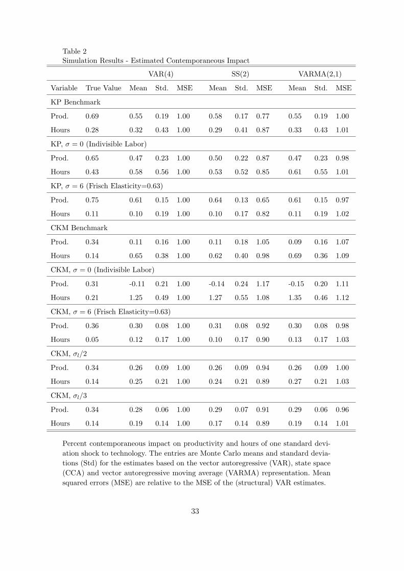
Table 2Simulation Results - Estimated Contemporaneous Impact

VAR(4) SS(2) VARMA(2,1)

Variable True Value Mean Std. MSE Mean Std. MSE Mean Std. MSE

KP Benchmark

Prod. 0.69 0.55 0.19 1.00 0.58 0.17 0.77 0.55 0.19 1.00

Hours 0.28 0.32 0.43 1.00 0.29 0.41 0.87 0.33 0.43 1.01

KP, σ = 0 (Indivisible Labor)

Prod. 0.65 0.47 0.23 1.00 0.50 0.22 0.87 0.47 0.23 0.98

Hours 0.43 0.58 0.56 1.00 0.53 0.52 0.85 0.61 0.55 1.01

KP, σ = 6 (Frisch Elasticity=0.63)

Prod. 0.75 0.61 0.15 1.00 0.64 0.13 0.65 0.61 0.15 0.97

Hours 0.11 0.10 0.19 1.00 0.10 0.17 0.82 0.11 0.19 1.02

CKM Benchmark

Prod. 0.34 0.11 0.16 1.00 0.11 0.18 1.05 0.09 0.16 1.07

Hours 0.14 0.65 0.38 1.00 0.62 0.40 0.98 0.69 0.36 1.09

CKM, σ = 0 (Indivisible Labor)

Prod. 0.31 -0.11 0.21 1.00 -0.14 0.24 1.17 -0.15 0.20 1.11

Hours 0.21 1.25 0.49 1.00 1.27 0.55 1.08 1.35 0.46 1.12

CKM, σ = 6 (Frisch Elasticity=0.63)

Prod. 0.36 0.30 0.08 1.00 0.31 0.08 0.92 0.30 0.08 0.98

Hours 0.05 0.12 0.17 1.00 0.10 0.17 0.90 0.13 0.17 1.03

CKM, σl/2

Prod. 0.34 0.26 0.09 1.00 0.26 0.09 0.94 0.26 0.09 1.00

Hours 0.14 0.25 0.21 1.00 0.24 0.21 0.89 0.27 0.21 1.03

CKM, σl/3

Prod. 0.34 0.28 0.06 1.00 0.29 0.07 0.91 0.29 0.06 0.96

Hours 0.14 0.19 0.14 1.00 0.17 0.14 0.89 0.19 0.14 1.01

Percent contemporaneous impact on productivity and hours of one standard devi-ation shock to technology. The entries are Monte Carlo means and standard devia-tions (Std) for the estimates based on the vector autoregressive (VAR), state space(CCA) and vector autoregressive moving average (VARMA) representation. Meansquared errors (MSE) are relative to the MSE of the (structural) VAR estimates.

33

Table 3Simulation Results - Estimated Long-Run Effect

VAR(4) SS(2) VARMA(2,1)

Variable True Value Mean Std. MSE Mean Std. MSE Mean Std. MSE

KP Benchmark

Prod. 1.17 1.01 0.39 1.00 0.91 0.23 0.68 1.01 0.39 0.99

Hours 6.66 12.38 22.40 1.00 8.92 14.58 0.41 12.93 22.49 1.02

KP, σ = 0 (Indivisible Labor)

Prod. 1.17 1.04 0.39 1.00 0.95 0.28 0.75 1.05 0.40 1.04

Hours 8.71 19.88 26.50 1.00 15.28 18.47 0.46 20.80 26.91 1.05

KP, σ = 6 (Frisch Elasticity=0.63)

Prod. 1.17 1.01 0.39 1.00 0.91 0.23 0.67 1.01 0.40 1.04

Hours 3.10 5.15 12.57 1.00 3.37 6.81 0.29 5.10 12.42 0.98

CKM Benchmark

Prod. 0.57 0.47 0.11 1.00 0.46 0.11 1.12 0.48 0.10 0.91

Hours 3.23 8.26 6.00 1.00 7.80 5.70 0.87 8.66 5.92 1.05

CKM, σ = 0 (Indivisible Labor)

Prod. 0.57 0.53 0.13 1.00 0.53 0.15 1.33 0.54 0.13 0.91

Hours 4.22 14.42 8.69 1.00 14.68 8.51 1.01 15.32 8.55 1.09

CKM, σ = 6 (Frisch Elasticity=0.63)

Prod. 0.57 0.42 0.08 1.00 0.41 0.06 1.03 0.42 0.07 0.96

Hours 1.50 1.64 2.48 1.00 1.45 2.30 0.86 1.73 2.42 0.96

CKM, σl/2

Prod. 0.57 0.43 0.09 1.00 0.42 0.08 1.03 0.43 0.08 0.93

Hours 3.23 3.37 2.98 1.00 3.01 2.86 0.92 3.48 2.94 0.98

CKM, σl/3

Prod. 0.57 0.43 0.10 1.00 0.42 0.08 1.03 0.43 0.09 0.95

Hours 3.23 2.65 2.26 1.00 2.31 2.03 0.92 2.69 2.22 0.97

Percent long-run effect on productivity and hours of one standard deviation shockto technology. The entries are Monte Carlo means and standard deviations (Std)for the estimates based on the vector autoregressive (VAR), state space (SS) andvector autoregressive moving average (VARMA) representation. All statistics arecomputed over 4% trimmed estimation results. See the text for explanation. Meansquared errors (MSE) are relative to the MSE of the (structural) VAR estimates.

34