BUREAU OF THE CENSUS

STATISTICAL RESEARCH DIVISION REPORT SERIES

SRD Research Report Number: CENSUS/SRD/RR-84116

TIME SERIES MOIJELING OF MONTHLY GENERAL

FERTILITY RATES

Robert 9. Miller and Sandra K. McKenzie ASA/Census Fellow Statistical Research Division Bureau of the Census Bureau of the Census Room 3524, F.O.B. #3 Room 3524, F.O.B. #3 Washington, D.C. 20233 Washington, D.C. 20233

(301) 763-3847 (301)763-7359

This series contains research reports, written by or in cooperation with staff members of the Statistical Research Division, whose content may be of interest to the general statistical research community. The views re- flected in these reports are not necessarily those of the Census Bureau nor do they necessarily represent Census Bureau statistical policy or prac- tice. Inquiries may be addressed to the author(s) or the SRD Report Series Coordinator, Statistical Research Division, Rureau of the Census, Washington, D.C. 20233.

Recommended by: Kirk M. Wolter

Report completed: August 6, 1984

Report issued: August 6, 1984

WORKING PAPER 884

Time Series Modeling of Monthly General

Fertility Rates

Robert 9. Miller*

Sandra K. McKenzie**

ABSTRACT

An analysis of monthly 1J.S. general fertility rates, 1950-1983, reveals (a) significant calendar effects, (b) seasonality, (c) outliers, (d) significantly different behavior over different decades, (e) the effect of benchmarking population figures to the 1980 census.

*ASA/Census Fellow, U.S. Bureau of the Census and Professor of Business and Statistics, University of Wisconsin, Madison

**Mathematical Statistician, U.S. Bureau of the Census

I. Introduction

The data in this study are monthly U.S. general fertility

rates, i.e., number of births divided by number of women aged

15-44, for January, 1950, through September, 1983. The data

through December, 1981, are final, whereas the data for 1982 and

1983 are provisional. The source of the data is the National

Center for Health Statistics (NCHS).

Population Division personnel at the U.S. Bureau of the

Census use these data for three major activities.

(a>

w

(4

In

Monthly estimates of annual rates are made to look for

early warning signals that previous projections of

annual rates and actual annual rates may differ

substantially.

Forecasts of monthly rates must be made to prepare new

demographic projections because the current population

estimates done by Census are more up-to-date than the

birth data that come from NCHS. (This is not a

criticism. The NCHS data depend on monthly reports from

states, which can be rather slow in coming in.

Compilation also takes time.)

Each month, l-, 2-, and 3-month ahead forecasts of birth

totals are formed and used as controls in planning the

Current Population Survey.

applications (a) and (c), decisions need to be made

quickly, but the most recent data available are only

2

provisional. Thus it is important to discover the relationships,

if any, between provisional and final data. Before such

relationships can be studied, however, it is necessary to

understand the stochastic behavior of the final data, which is

the topic of this paper.

Questions of scientific interest arise concerning these

final general fertility rates.

(a) Has the stochastic behavior of rates changed over time?

(b) Are there deterministic sources of variation in the

rates, e.g. calendar effects, lunar effects, and

benchmarking of population estimates to different

censuses in different decades?

(c) To what extent are monthly rates seasonal?

(d) Are outliers many or few?

In this paper we will address some, but not all, of the questions

raised above. Our major conclusions are that monthly general

fertility rates are seasonal, calendar effects are significant,

outliers are few, and the stochastic (ARMA) behavior of the rates

changes over time.

II. Preliminary Modeling

The Box-Jenkins model building prescription of identification,

estimation, and checking was applied to the data for the decades

of the 50's, 60's, and 70's separately. Natural logarithms of

the fertility rates were modeled to eliminate heteroscedasticity.

Inspection of a plot of the natural logarithms (Figure 1)

revealed the changing character of the series over time.

Modeling relatively homogeneous segments of the data seemed

appropriate, especially in light of changing social and cultural

influences (see, for example, Freedman (1979), Lee (1975), Ryder

(1979), Tu and Herzfeld (1982), and Westhoff (1983)). Moreover,

the population totals in the denominators of the general

fertility rates are benchmarked to the most recent past census,

so partitioning the data into decades makes sense.

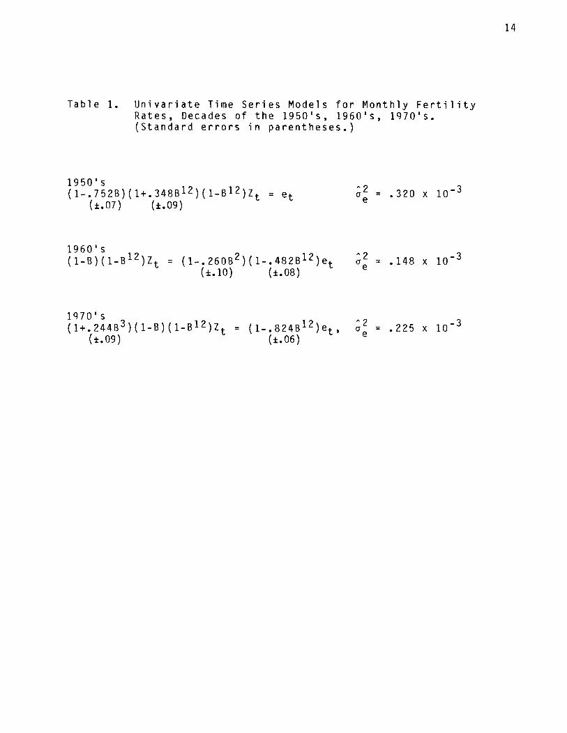
The models thus obtained are displayed in Table 1. Note the

difference in the model forms among the three segments, even at

this preliminary stage of model identification. The associated

residual autocorrelation functions have prominent spikes at an

unusual set of lags: 14, 19, 21, 23, 27, 29, and 33 (see Figure

2). Our experience is that calendar variation is often

associated with autocorrelation at otherwise inexplicable lags.

[See Bell and Hillmer (1983) for a discussion of the effects of

calendar variation.] The presence of calendar variation in

fertility data is well documented. See Menaker and Menaker

(1959) and Criss and Marcum (1981). Land and Cantor (1983)

attempted a crude calendar eff,ects analysis with ARIMA models,

but with unsatisfactory results.

Following Bell and Hillmer (1983), models with calendar

effects were fitted to the three decades of fertility rate

data. In their notation, six calendar variables have the form

(number of days of type i) minus (number of Sundays): Tl =

(number of Mondays) - (number of Sundays), . . . , T6 = (number of

4

Saturdays) - (number of Sundays). The seventh calendar variable

measures the length of the month: T7 = number of days in the

month. The program described by Bell (1983) was used to search

for outliers, and terms for prominent outliers were also included

in the models. An additive outlier (AO) is a pulse disturbance

in the data at a fixed epoch t0. A level shift (LS) outlier is a

permanent shift in level of the data. Bell's program searches

for these types of outliers (plus some others).

The models fitted to the 1960’s and 1970’s had the form

7 1-B)(1-B12)Zt = c BJ(

J=l 1-B) l-B12)TJt

(1)

+ c ai(l-B)(1-B12)~~i) + Nt i ~52

where Nt follows a stationary ARMA model, the TJ's are the

calendar variables, $1 is an appropriate outlier variable,

and R is the set of time epochs at which outliers occur. In the

model fitted to the 1950's the seasonality had to be handled

differently because attempts to include a seasonal difference and

a twelfth-order moving average parameter led to il2 = 1.00,

effecting a cancellation with the seasonal difference. This

indicated deterministic, rather than stochastic, seasonality.

Thus, the model for the 1950's has eleven seasonal indicators

Sl ,***, Sll (for the months January through November), a constant

term, and no seasonal difference. The model form is

7 (1-B)Zt = + C BJ(l-B)TJt

J=l

11 + C vs(l-B)Sst + (1-9)~~

s=l (2)

+ C cxi(l-B)$) + Nt i aS2

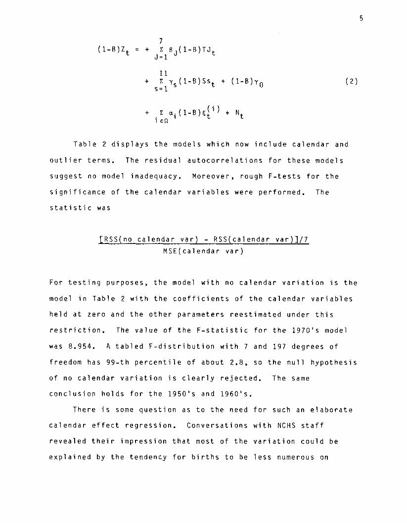
Table 2 displays the models which now include calendar and

outlier terms. The residual autocorrelations for these models

suggest no model inadequacy. Moreover, rough F-tests for the

significance of the calendar variables were performed. The

statistic was

[RSS(no calendar var) - RSS(calendar var)]/7

MSE(calendar var)

For testing purposes, the model with no calendar variation is the

model in Table 2 with the coefficients of the calendar variables

held at zero and the other parameters reestimated under this

restriction. The value of the F-statistic for the 1970's model

was 8.954. A tabled F-distribution with 7 and 197 degrees of

freedom has 99-th percentile of about 2.8, so the null hypothesis

of no calendar variation is clearly rejected. The same

conclusion holds for the 1950's and 1960's.

There is some question as to the need for such an elaborate

calendar effect regression. Conversations with NCHS staff

revealed their impression that most of the variation could be

explained by the tendency for births to be less numerous on

6

weekend days than on weekdays. Menaker and Menaker (1959) found

this effect more pronounced in private hospitals than in public

ones where doctors are on call 24 hours a day. See Criss and

Marcum (1981) and the references therein for extensive

documentation of the weekend effect.

If the weekday/weekend effect dominates the calendar

the simpler model variation, then we may use

(1-B )(l-B12)Z t

= 6 1 (1-B) (1-B12)Kt+62(1-B)(1-B12)Lt+Nt (3)

where Kt = the difference between the number of weekdays and the

number of weekend days in month t, Lt = the number of days in the

month (equal to T7 in model (l)), and Nt is stochastic noise with

ARMA structure. The model may contain outlier terms and again,

the model needs modification to handle the non-stochastic

seasonal in the 1950's.

In the models in Table 2 we replaced the seven-variable

calendar components with the simpler two-variable component of

equation (3) and reestimated the models. We then computed F-

statistics of the form

[RSS(2 calendar variables) - RSS(7 calendar variables)]/5

MSE(7 calendar variables)

These F-statistics for the 1950’s, 1960’s, and 1970's were 2.29,

1.16, and 0.56. They support the hypothesis that the simpler,

two-variable calendar component is a sufficient description of

the calendar variation in the monthly fertility rates.

Finally, we remodeled the data using the reduced calendar

component. The results are reported in Table 3.

III. Interpretation of Models

The models displayed in Table 3 are indeed different across

the three decades. This observation corresponds to the

qualitative impression mentioned earlier that one gets from a

plot of the general fertility rates. The 1950's are a period of

steady increase, the 1960's a period of rapid decrease, and the

1970's a perio,d of leveling off. The 1960's and 1970's models

both have the operator (l-B)(l-B12). The 1950's have a

deterministic seasonal pattern as well as calendar effects.

Comparison of Variance Estimates

If we compare the iz' s for the different models (compare

Tables 1 and 3), we see that the inclusion of calendar and

outlier variables substantially reduces the variance estimates

(48X, 15X, and 34% for the three decades). In the 1960's, going

from the full set of calendar variables to the reduced set

(compare Tables 2 and 3) results in a 16% increase in the

variance estimate, though the F-test did not reject a reduced

model. In the 1950's and 1970's the variance estimates for the

full and reduced calendar component models are not much

different.

Comparison of Parameter Estimates

Comparing the coefficients of the seven-variable calendar

component (ii 's in Table 2), we see that while the magnitudes of

the coefficients vary, in the two models for the 1960's and

1970's the signs of the coefficients are the same. The

8

coefficients BI, . ..B6 do not admit meaningful interpretations

individually, and must be considered as part of the overall

calendar effect. In contrast, the coefficients of the two-

variable calendar component (ii 's in Table 3) have a behavioral

interpretation as the impact of the weekend/weekday effect (;I)

and the adjustment for leap-year Februaries (i2) [see Bell and

Hillmer, (1983)]. Note again that the signs of 6I and i2 are the

same for the 1960's and 1970's.

The ARMA components of the models in Tables 2 and 3 are not

too similar for the 1960's and 1970's, as can be confirmed by

computing the Y-weights. Thus, the type of deterministic

calendar component specified in the model affects the

characterization of the stochastic structure of the series. In

addition, the type of ARMA model specified (possibly also the

type of calendar component used) affects the outlier detection --

slightly different sets of outliers for the 1960’s and 1970's are

specified in Tables 3 and 2. Thus, the ARMA components of the

models appear to interact with the calendar specification and the

detection of outliers.

In summary, our analysis in Section III has shown that the

monthly general fertility rates can be fitted by models that

a> display significant calendar effects primarily related

to differing numbers of births on weekdays and weekend

days

W display seasonality of deterministic type in the 1950’s

and of stochastic type in the 1960's and 1970's

c) are subject to very few outliers

9

d) differ substantially from decade to decade, suggesting

gradual behavioral shifts in the birth process over time

IV. The Effect of Benchmarking

Population estimates are benchmarked on the most recent past

census, which is taken in years ending in zero. Different

coverage rates in different censuses can cause variation in

population estimates, and hence in fertility rates, that are

unrelated to natural sources of variation. For example, coverage

rates for the 1980 census were, on the whole, higher than for

1970. This could result in an apparent increase in population

and decrease in fertility rates in the 1980's that is unrelated

to real population shifts.

4.1 Testing for the effect of benchmarking

We shall use a test proposed by Box and Tiao (1976) to look

for a shift between the 1970's and the 1980's. Only the 24

monthly observations from 1980 and 1981 will be used because this

exhausts the final data available.

The minimum mean squared error forecasts of the 1980 and

1981 data were generated from December, 1979, using the 1970's

model in Table 3. Let i2 denote the residual mean square, and

let al, . . . . a24 denote the forecast errors in 1980 and 1981.

Box and Tiao's test statistic is

24 Q = im2 C a:,

a=1

which is referred to a ~'(24) distribution for significance.

10

For our data the value of Q is 107.486. Because this

statistic is significant, it is very likely that the 1980's data

are different from those expected by extrapolating the 1970’s

model. Table 4, upper panel, shows the forecast errors and the

standard errors of these forecast errors estimated using the

1970's model. A time series plot of the forecast errors (Figure

3) reveals that the forecasts are unbiased through February,

1981, but they are too high for the rest of the period. This

suggests a level shift in the actual fertility rates which may or

may not be due to benchmarking. Our hypothesis was that the

benchmarking effect would show up as a level shift beginning in

early 1980. The apparent shift in the data, which begins with

March, 1981, could be signalling a change in the stochastic

behavior of the data. As we have documented changing ARMA

behavior across previous decades, we must admit that such changes

could be confounded with any level shifts that may be present.

Another test for model shifts can be performed as follows.

Fit the 1970’s model in Table 3 to the data from l/70 through

12181. (Remember that 12/81 is the end of the final data series

now available.) Part of the fitting process is to run Bell's

(1983) outlier program which will presumably detect shifts. When

this procedure was carried out, the program detected A0 outliers at

2/81 and 11/81. The presence of an outlier at 2/81 corresponds

to the impression we got from the forecast error plot that some

change from the underlying 1970’s model had occurred. How a

certain kind of outlier in the series relates to the forecast

errors is a question that will be addressed in a later paper.

11

Regardless of the details, however, the main conclusion is

clear. We would be reluctant to use the 1970's model for data in

the 1980's without some further modification.

4.2 Contrast with simple ARMA analysis

What would have been our conclusion if we had used the ARMA

model in Table 1 (which lacks a calendar component) as our 1970's

model? The Q statistic is 939.775, indicating a major shift and

agreeing with the analysis in Section 4.1. Table 4, bottom

panel, shows the forecast errors and their estimated standard

errors for the Table 1 model. Twenty-one out of 24 errors are

positive, indicating forecasts that are too low throughout

1980-81. Figure 3 shows the contrast between forecast errors

from the two models. The results from the simple ARMA model of

Table 1 suggest a level shift in the opposite direction

anticipated by our benchmarking discussion and actually found

after fitting calendar components! Thus, ignoring calendar

variation in time series analysis would have resulted in

erroneous conclusions.

v. Comparison with Land and Cantor

Land and Cantor (1983) presented an analysis of general

fertility rates over the period 1950-1979. Our study differs

from theirs in several important respects.

1. We checked for varying model form over time.

2. Our incorporation of calendar components from the time

series literature was successful in modelling the

12

calendar effect.

The attempts of Land and Cantor to account for the

calendar components by the operator (l-B13) on the left-

hand-side of their equation, induced the need for MA

terms at lags 13, 14 and 15.

3. Our method of incorporating the calendar component led

to forecasts which are not misleading for the out-of-

sample period of the early 1980's.

Land and Cantor concluded that using the (l-B13)

operator was not an improvement, and the model with that

operator exhibited inferior forecasting performance for

the within-sample period December, 1976 to December,

1978.

VI. Conclusions

We have presented a model for monthly general fertility

rates that includes a nonstochastic regression component to

capture calendar effects and outliers and an ARIMA component to

capture stochastic effects. These components are estimated

jointly using efficient statistical methods that allow us to test

for the significance of the various effects. Our approach would

allow other nonstochastic components to be added to the model and

tested for significance. We have shown how our comprehensive

model can be used to detect shifts in the data and how less

comprehensive models can lead to erroneous conclusions.

13

REFERENCES

Bell, W.R. (1983). A Computer Program for Detecting Outliers in Time Series. Proceedings of the Business and Economics Statistics Section, American Statistical Association, Washington, D.C. pp. 634-639.

Bell, W.R. and Hillmer, S. (1983). Modeling Time Series with Calendar Variation. Journal of the American Statistical Association, 78, 526-534.

Box, G.E.P. and Tiao, G.C. (1976). Comparison of Forecast and Actuality, Applied Statistics, 25, 195-200.

Criss, T.B. and Marcum, J.P. (1981). A Lunar Effect on Fertility. Social Biology, 28, 75-80.

Freedman, Ronald (1979). Theories of Fertility Decline: A Reappraisal. Social Forces, 58, 1-17.

Land, K.C. and Cantor, D. (1983). ARIMA Models of Seasonal Variation in U.S. Birth and Death Rates. Demography, 20 -' 541-568.

Lee, Ronald D. (1975). Natural Fertility, Population Cycles and the Spectral Analysis of Births and Marriages. Journal of the American Statistical Association, 70, 295-304.

W-w, G. and Box, G. (1978). On a Measure of Lack of Fit in Time Series Models. Biometrika, 65, 297-304.

Menaker, W. and Menaker, A. (1959). Lunar Periodicity in Human Reproduction: A Likely Unit of Biological Time. American Journal of Obstetric Gynecology, 77, 905-914.

Ryder, Norman B. (1979). The Future of American Fertility. Social Problems, 26, 359-370.

Tu, Edward J-C. and Herzfeld, Peter M. (1982). The Impact of Legal Abortion on Marital and Nonmarital Fertility in Upstate New York. Family Planning Perspectives, 14, 37-46.

Westoff, Charles F. (1983). Fertility Decline in the West: Causes and Prospects. Population and Development Review, 2, 99-104.

14

Table 1. Univariate Time Series Models for Monthly Fertility Rates, Decades of the 1950’s, 1960’s, 1970’s. (Standard errors in parentheses.)

;2 = . 320 x 1O-3 e

1950’s (1-;75::))( l+.(i4ii)12) (l-B12)Zt = et

f. .

1960’s (~-B)(I-B~~)Z t = (l- 260B2)(1-.482B12)e

ik. 10) A2 = .148 x 10’~

(~08) ’ ae

1970’s (1+.244B3)(1-B)(l-Bl2)Z

b.09) t = (l- 824B12)e A2 = .

ik.06) ” ue 225 x 1O-3

15

Parameter Estimate St. Err Estimate St. Err Estimate St. Err

%

82

$3

84

85

'6

87

al

a2

yO

y1

y2

y3

y4

y5

'6

y7

'8

y9

y10

yll

Table 2. Models with Seven Calendar Variables and Outlier Variables, Decades of 195,0's, 1960's, 1970's. (Standard-errors in parentheses.)

Decade

1950'S 1960's 1970's

.0022 .0020

.0037 .0020

-.0036 .0020

.0020 .0020

.0039 .0020

-.0051 .0020

-.0058 .0067

.0009 .0004

-.0245 .0059

-.0195 .0157

-.0204 .0059

-.0742 .0054

-.0587 .0059

-.0118 .0054

.0459 .0059

.0650 .0059

.0767 .0054

.0313 .0059

-.0061 .0054

-.OOOl .0013

.0018 .0013

.0028 .0013

-.0014 l 0012

.0017 .0013

-.0016 .0012

.0051 .0037

-.0173 .0058

-.0205 .0061

Outliers: None AOJune62 AOApri167

Noise models: 1950's Nt = (l-.4349B2-.2442B3)et,

(~082) (~083)

1960's Nt =

1970's Nt =

-.0003 .0018

.0050 .0017

.0009 .0018

-.0005 .0018

.0033 .0017

-.0035 .OOll

.0021 .0064

-.0416 .0124

LSNov71

;2 = e .157 x 10'3

1+.2157B-.0269B2 -.3811B3)(1- 5483B12), i2 = .108 x lO-3 (k.093) (k.095) (*.099) l (k.078) e

1 7849R12)e -'(*.0668) lz'

;2 = e

.149 x 10'3

16

Table 3. Models with Two Calendar Variables and Outlier Variables.

Parameter

5

62

"1

yO

y1

y2

y3

y4

y5

'6

y7

y8

y9

ylo

yll

Outliers

Decades of 1950's, 1960's, 1970's. (Standard errors in parentheses.)

Decade

1950's 1960's 1970's

Estimate St. Err

.0018 .0004

-.0004 .0069

.0009 l 0004

-.0233 .0060

-.0237 .0160

-.0192 .0060

-.0755 .0055

-.0577 .0060

-.0121 .0055

.0470 .0060

.0657 .0060

.0758 .0055

.0323 .0060

-.0066 .0055

None AOApri167 None

Estimate St. Err

.0017 .0003

.0032 .0042

-.0239 .0069

Noise models: 1950's Nt = (l-.4207B2-.2551B3)et,

(k.0800) (~080)

1960's % = (l-ct3~~~3)(1-.477B12)et, . (~08)

Estimate St. Err

.0028 .0003

.0022 .0053

;2 = e

.166 x 1o-3

;2 = e ’ 125 x 1O-3

1970's (l+ 490B12)N (*.09) t

= (l- 216B2)(1- 32B12)e (*ho) (hio)

;2 = t' e

.148 x 1O-3

z w

e

- . .

00

CnN

m

w

IUP

V

- l

.

OW

zs

OYLI

V

-

.

.

00

AW

ix

- - . .

00

AN

Ln

w

r-h

V

- . .

00

4-B

w

r N

Ln

- - . .

00

co-

Pen

W

+ - - .

. O

l- w

w

Pl-

r\)cr

, - - .

. O

l- co

4 +I

- O

W

- - . .

Oi-

030-

f W

N

4w

- - . .

00

wm

N

O

W*

-1 .

. 00

W

O

PN

w

wl

- . .

00

wo

403

PW

z 0

-1 .

. 00

‘-

0 m

m

OU

I - - .

. 30

N

rn

V

- . .

00

x3-h

ho

-3

003

V

- . .

00

WC

n ‘V

W

04

- - . .

00

ww

40

7 ow

- - .

. 00

PW

zz

- - . .

OW

P

m

CnW

P-

F-

- . .

OW

Pe

n w

w

C-IW

V

- . .

OW

cn

cn

NW

U

lW

- - . .

00

CnW

C

nN

-JO

Y

- -1 .

. 00

:z

ww

V

-1

. .

00

m0

‘-JN

-C

o -

-

< ID

W

7 +

N

W

P

cn

3 -n

0 3 s:

rt

3

J

-I

W

o-

z c-’

Figure 1: Natural logarithms of monthly general fertility rates, 1950-1979

08 8f 8L Lf BL Sf PL Et ZL IL 0f

0L 83 33 LB 93 SB PB 89 29 13 09

080-b I 080’tr

00S’b-- S0961

-00S’*

060’S 000’S

03 8s 3s LS 9s ss PS 6s 2s IS 0s

000’lr I 000’P

Si10S61 BBS’+-- -00S’tr

000 ‘S 000’9

3WXKl A8 S3lW A.i.111183~ AlHlNOW JO WHlItiV9Ol lWH-UVN

Figure 2. Sample Autocorrelation Function of Residuals from 1970's Model in Table 1. (Dotted lines are approximate long-lag two standard error limits.)

---.-...-I___.-_-.------- ------.-Is-

-00.0

--ST0

-0s.0

-SL’B

?- 3'lW.l WO&J 13aOW L0l.61 'NOIJJNfld. NOI.lW'l3tl~O3OJJlW 3WfKIIS3tl

Figure 3. Time Series Plots of Forecast Errors, 1980-81. Forecasts from: a) 1970's Model in Table 3 (dotted line) b) 1970's Model in Table 1 (solid line)

Y

\ . , , I , I ; I I , ,