bulk metal forming ii - rwth aachen university metal forming ii simulation techniques in...

© WZL/Fraunhofer IPT

Bulk Metal Forming II

Simulation Techniques in Manufacturing Technology

Lecture 2

Laboratory for Machine Tools and Production Enginee ring

Chair of Manufacturing Technology

Prof. Dr.-Ing. Dr.-Ing. E.h. Dr. h.c. Dr. h.c. F. Klocke

Seite 1© WZL/Fraunhofer IPT

Lecture objectives

� Overview of analytic and numeric methods in process modelling

� Introduction and fundamentals in Finite Element Modelling

� Examples of process simulations in bulk forming

� Overview of damage mechanisms and damage modelling in bulk forming

� Future developments in bulk forming simulation


Summary5

Future Developments4

Examples3

Simulation of bulk forming2

Fundamentals of FEM-Simulations1

Outline


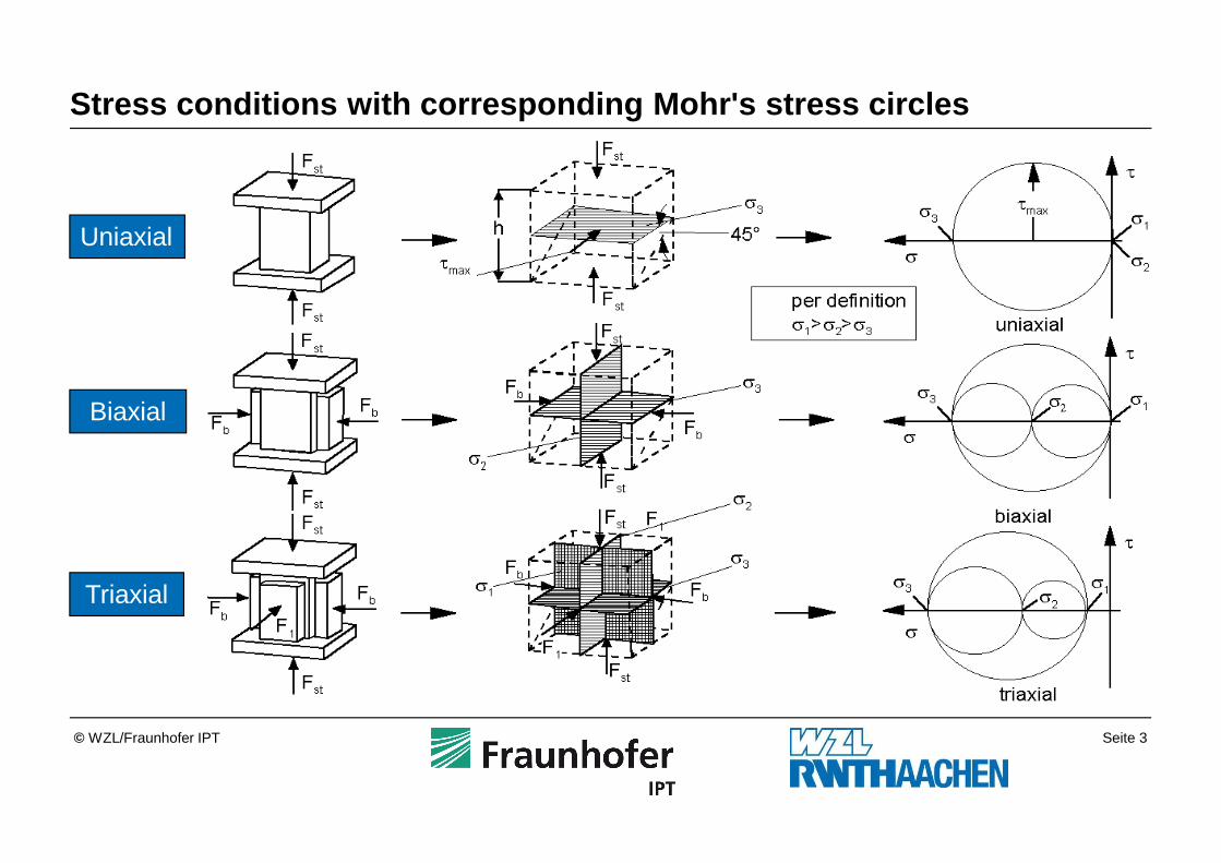
Stress conditions with corresponding Mohr's stress circles

Uniaxial

Biaxial

Triaxial


Start of yielding


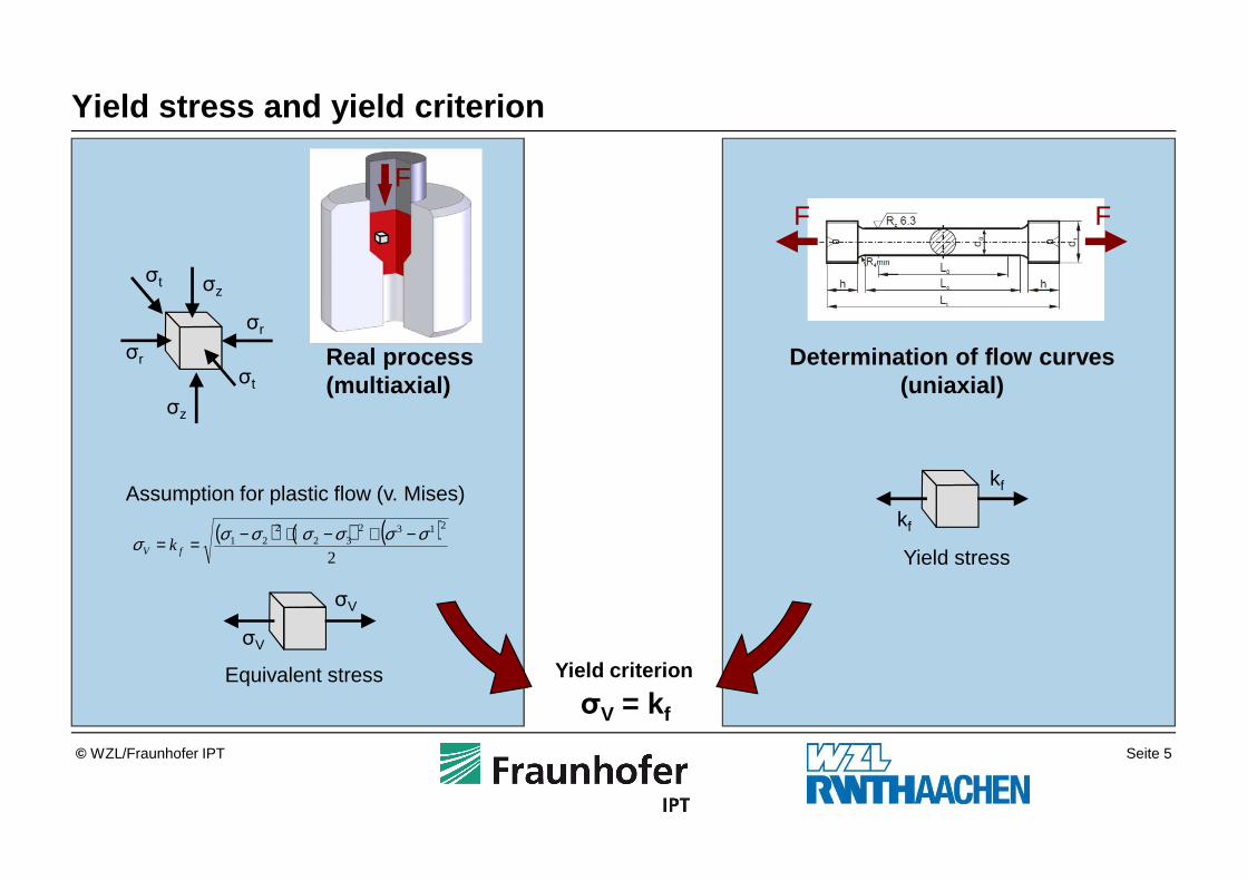
Yield stress and yield criterion

σr

σr

σz

σz

σt

σt

Assumption for plastic flow (v. Mises)

( ) ( ) ( )2

213232

221 σσσσσσσ −+−+−== fV k

σV

σV

Equivalent stress Yield criterion

σV = k f

F F

kf

Yield stress

kf

Real process(multiaxial)

Determination of flow curves(uniaxial)

F


( ) ( ) ( )2

213232

221 σσσσσσσ −+−+−== fV k

kf

-kf

σ3-σ3

σ1

-σ1

kf

-kf

σ2=0

von Mises

Tresca

σ1σ3 σ2

τ

τ

σ1σ3

σ2

τmax

von Mises

Tresca

Demonstration of the two yield criterions in ayield locus diagram for the state of plane stress.

fV k==−= max31 2τσσσ

Comparison of the yield criterions according von Mi ses and Tresca

Yield begin: wdeviatoric reaches critical value

Yield begin: shear stress τmax reaches shear yield k


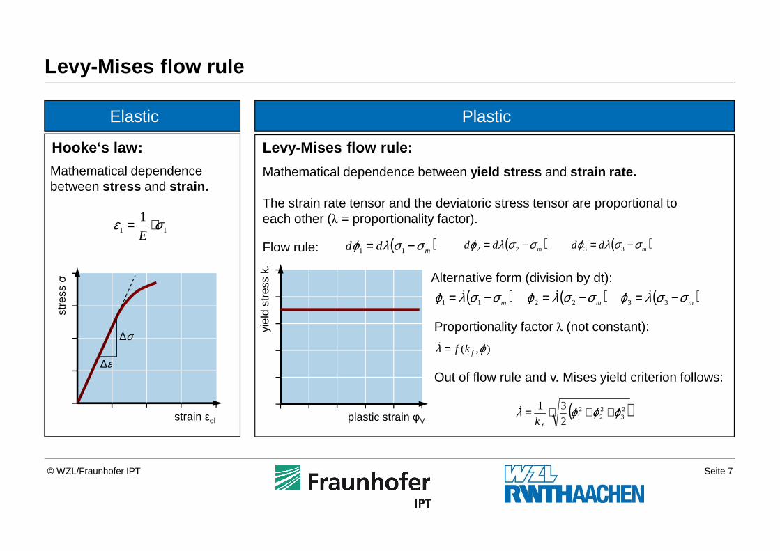
The strain rate tensor and the deviatoric stress tensor are proportional toeach other (λ = proportionality factor).

Levy-Mises flow rule

Elastic Plastic

11

1 σε ⋅=E

Hooke‘s law:

stre

ss σ

strain εel

ε∆

σ∆),( ϕλ &&

fkf=

Levy-Mises flow rule:

Mathematical dependence between yield stress and strain rate.

( )23

22

212

31 ϕϕϕλ &&&& ++⋅=fk

( )mσσλϕ −= 11&& ( )mσσλϕ −= 22

&& ( )mσσλϕ −= 33&&

Proportionality factor λ (not constant):

Mathematical dependence between stress and strain.

Alternative form (division by dt):

Out of flow rule and v. Mises yield criterion follows:

( )mdd σσλϕ −= 22( )mdd σσλϕ −= 11( )mdd σσλϕ −= 33Flow rule:

yiel

d st

ress

kf

plastic strain φV


Calculation methods in plasticity theory

„elementary“ plasticity theory plasticity theory

analytical methods

energy method

stripe model

disk model

tube model

strict solution

slip field calculation

graphical-, empirical-,analytical method

viscoplasticity

numerical methods

upper and lower bound method

error compensation method

finite element method

based on simplifications

based on theory

closed solution approximate solution


Analytical calculation methods with the stripe-, di sk- and tube model

strip

stripe modeltube model

tube

disk model

disk


� Equilibrium condition in drawing direction:

� Yield criterion according to Tresca with p (compressive stress) and σz (tensile stress) ≥ 0:

� Elimination of p results in a differential equation of 1st order:

Disk model

( ) 01 =+++ αµσσ cotpdAd

A zz

fz kp =+ σ

( )0

1 =++−A

cotkA

cotdAd f

zz αµσαµσ

Example: drawing of rods or wire

( ) ( ) 0=++′ xgxf zz σσ

A0

A1

AA + dAareas:

Fσzσz + dσz

α

pµ p

α

Source: Pawelski, O. (1976)

Assumptions: vz(r) = const.vz(z) ≠ const.

die

workpiece


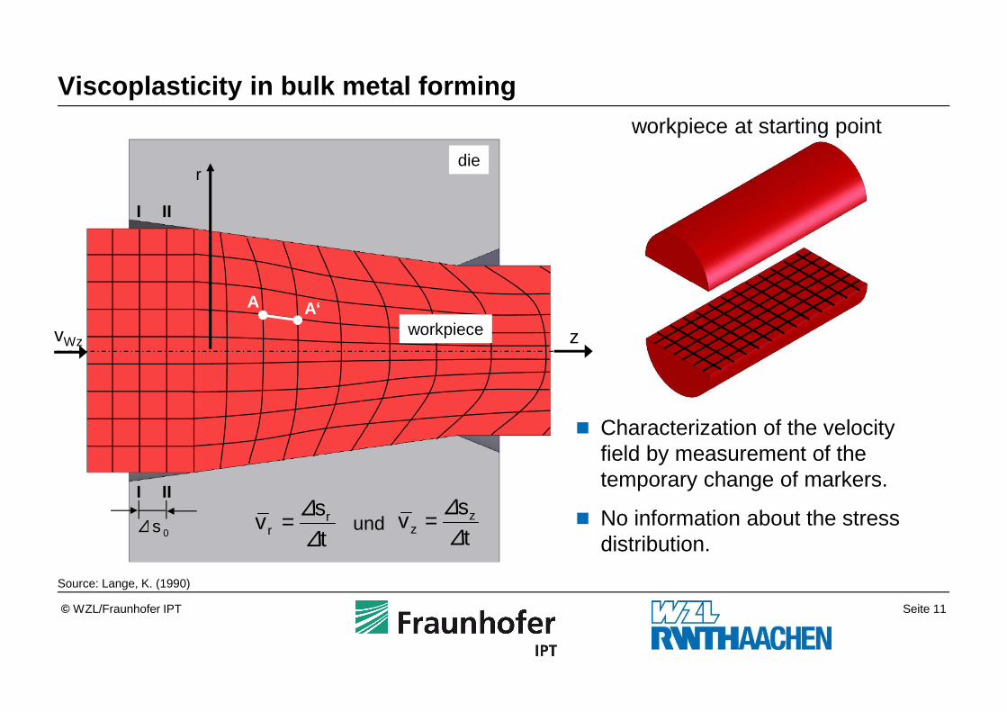
Viscoplasticity in bulk metal forming

Source: Lange, K. (1990)

� Characterization of the velocity field by measurement of the temporary change of markers.

� No information about the stress distribution.

ts

v r

∆∆=

A A‘

zvWz

r

ts

v zz ∆

∆=ts

v rr ∆

∆= und

die

workpiece

I II

I II

0s∆

workpiece at starting point


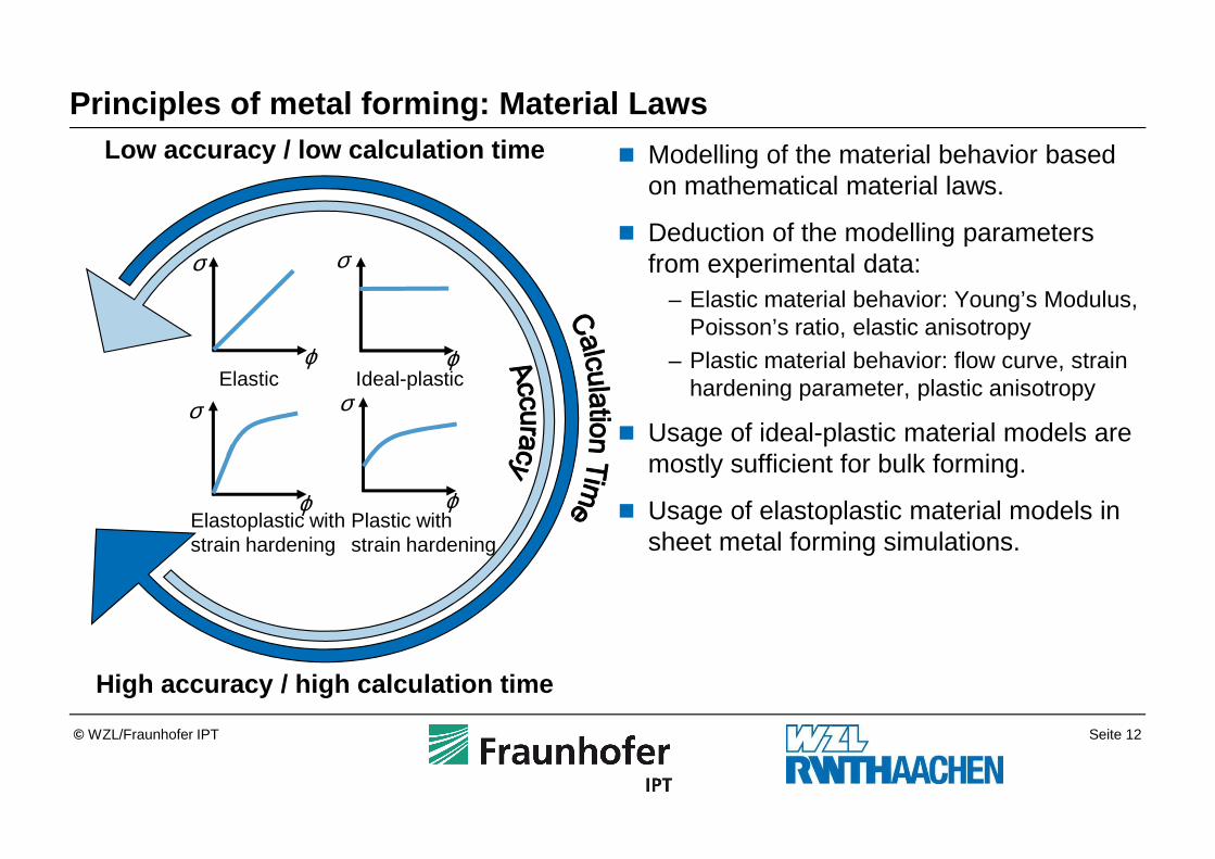
Principles of metal forming: Material Laws

� Modelling of the material behavior based on mathematical material laws.

� Deduction of the modelling parameters from experimental data:

– Elastic material behavior: Young’s Modulus, Poisson’s ratio, elastic anisotropy

– Plastic material behavior: flow curve, strain hardening parameter, plastic anisotropy

� Usage of ideal-plastic material models are mostly sufficient for bulk forming.

� Usage of elastoplastic material models in sheet metal forming simulations.

Elastic

σ

ϕIdeal-plastic

σ

ϕ

Plastic withstrain hardening

σ

ϕElastoplastic withstrain hardening

σ

ϕ

Low accuracy / low calculation time

High accuracy / high calculation time


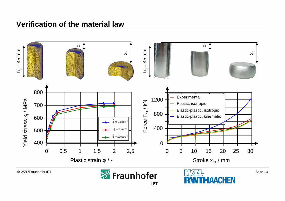
Verification of the material law

)(f nibRe σ=τ

h 0=

45

mm

x 1

x 2

Yie

ld s

tres

s k f

/ MP

a

For

ce F

St/ k

N400

500

600

700

800

0

400

800

1200

0 0,5 1 1,5 2 2,5 0 5 10 15 20 25 30

Stroke xSt / mmPlastic strain φ / -

1sec1,0 −•

=ϕ

1sec1 −•

=ϕ

1sec10 −•

=ϕ

Experimental

Plastic, isotropic

Elastic-plastic, isotropic

Elastic-plastic, kinematic

h 0=

45

mm

x 1

x 2


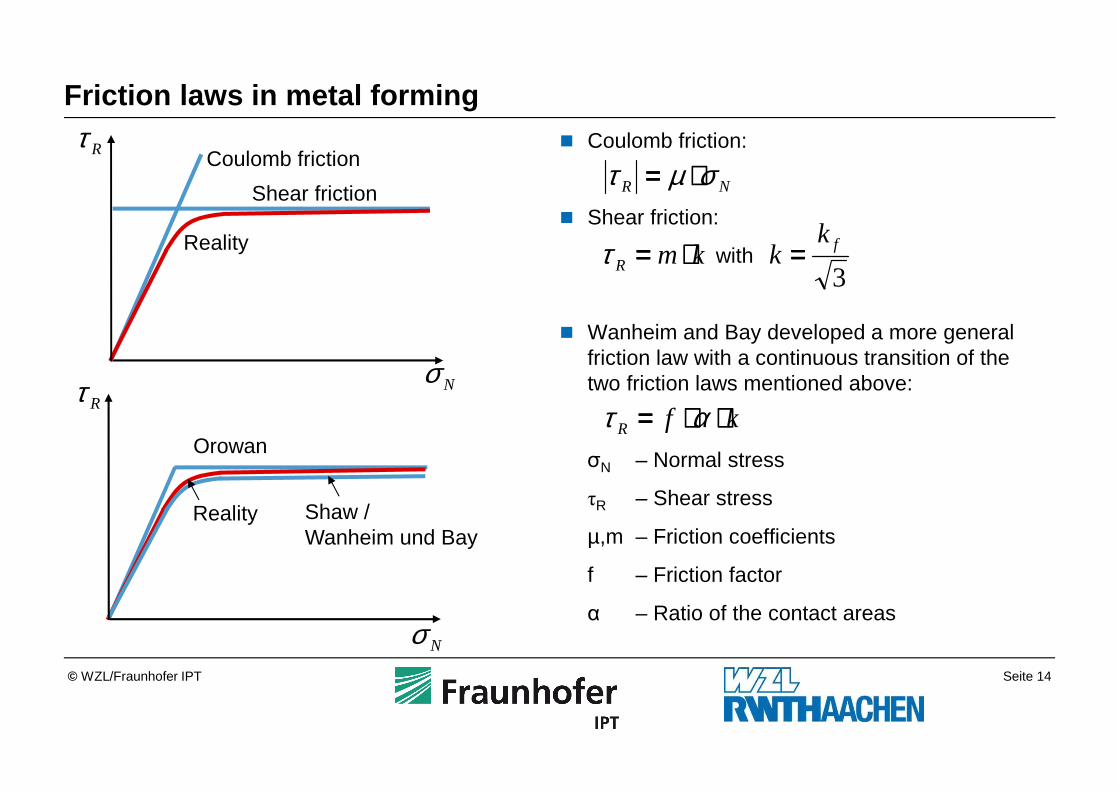
Friction laws in metal forming� Coulomb friction:

� Shear friction:

with

� Wanheim and Bay developed a more general friction law with a continuous transition of the two friction laws mentioned above:

σN – Normal stress

τR – Shear stress

µ,m – Friction coefficients

f – Friction factor

α – Ratio of the contact areas

Coulomb friction

Shear friction

Reality

Orowan

Shaw / Wanheim und Bay

Reality

Nσ

Nσ

Rτ

Rτ

NR σµτ ⋅⋅⋅⋅====

kmR ⋅⋅⋅⋅====τ3fk

k ====

kfR ⋅⋅⋅⋅⋅⋅⋅⋅==== ατ


Summary5


Examples3



Outline


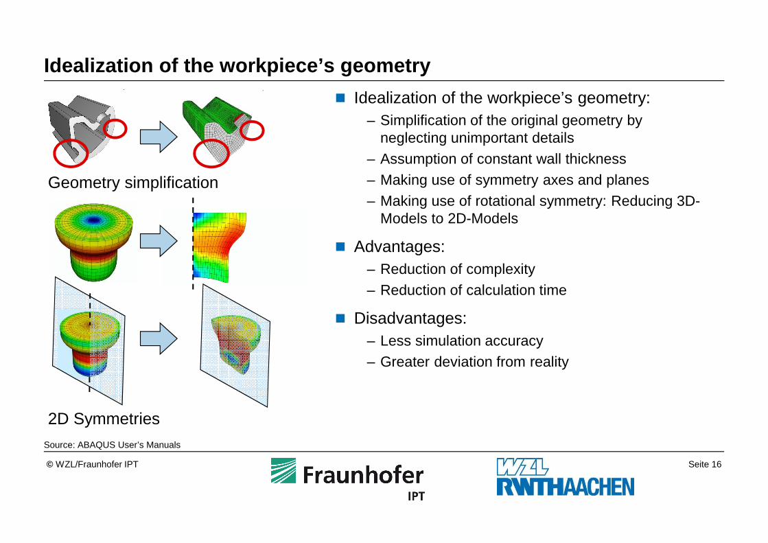
Idealization of the workpiece’s geometry

� Idealization of the workpiece’s geometry:– Simplification of the original geometry by

neglecting unimportant details– Assumption of constant wall thickness– Making use of symmetry axes and planes– Making use of rotational symmetry: Reducing 3D-

Models to 2D-Models

� Advantages:– Reduction of complexity– Reduction of calculation time

� Disadvantages:– Less simulation accuracy– Greater deviation from reality

Source: ABAQUS User’s Manuals

Geometry simplification

2D Symmetries


Type of elements

1D

2D

3D

Dimension Element type (load) Geometry

Rod (strain)

Beam (strain, bending)Membrane (2-dim. strain)Shell (strain, bending)

Volume element (strain)

Tetrahedron Pyramid HexahedronPentahedron


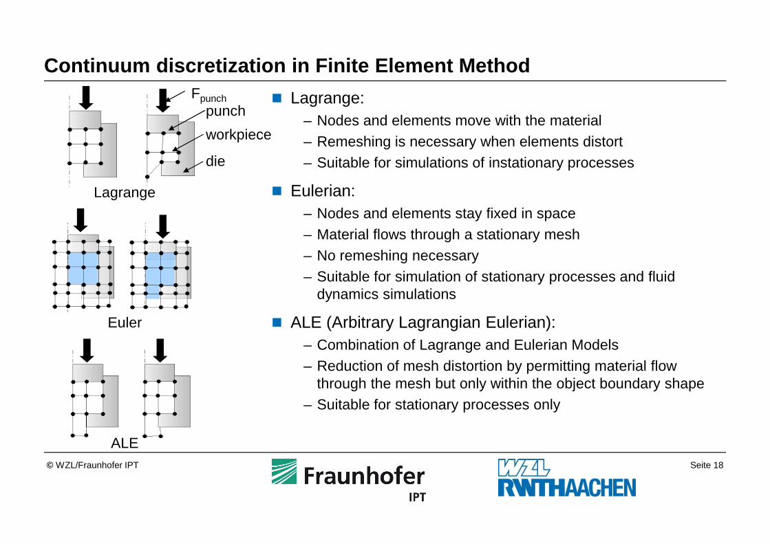
Continuum discretization in Finite Element Method

� Lagrange:– Nodes and elements move with the material– Remeshing is necessary when elements distort – Suitable for simulations of instationary processes

� Eulerian:– Nodes and elements stay fixed in space– Material flows through a stationary mesh– No remeshing necessary– Suitable for simulation of stationary processes and fluid

dynamics simulations

� ALE (Arbitrary Lagrangian Eulerian):– Combination of Lagrange and Eulerian Models– Reduction of mesh distortion by permitting material flow

through the mesh but only within the object boundary shape– Suitable for stationary processes only

Lagrange

Euler

ALE

Fpunchpunch

workpiece

die


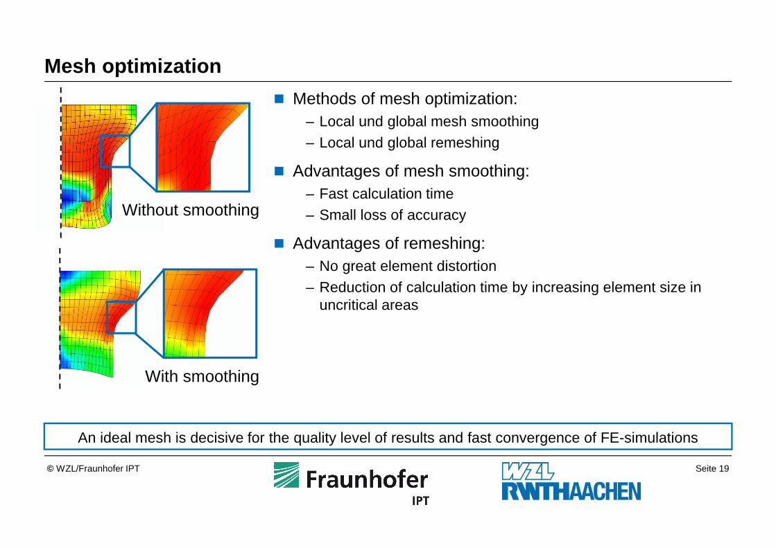
Mesh optimization

� Methods of mesh optimization:– Local und global mesh smoothing– Local und global remeshing

� Advantages of mesh smoothing:– Fast calculation time– Small loss of accuracy

� Advantages of remeshing:– No great element distortion– Reduction of calculation time by increasing element size in

uncritical areas

Without smoothing

With smoothing

An ideal mesh is decisive for the quality level of results and fast convergence of FE-simulations


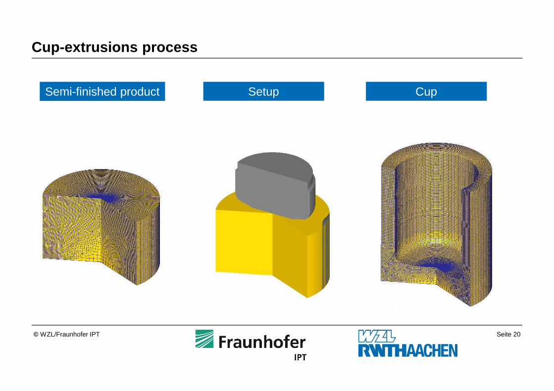
Cup-extrusions process

Semi-finished product Setup Cup


Cup-extrusions process: effective strain, effective strain rate

1.0

0.2

0.6

0.8

Effective strain φV

0

3

φV

Effective strain rate dφV/dt

0

2

dφV/dt


Cup-extrusions process: mean stress, effective stre ss

1.0

0.2

0.6

0.8

Mean stress σm

-2000

300

σV,

MP

a

Effective stress σV

0

800

σm, M

Pa


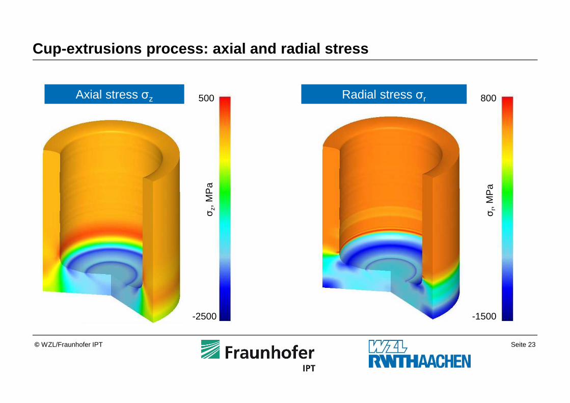
Cup-extrusions process: axial and radial stress

1.0

0.2

0.6

0.8

Axial stress σz

-2500

500

σr,

MP

a

Radial stress σr

-1500

800

σz,

MP

a


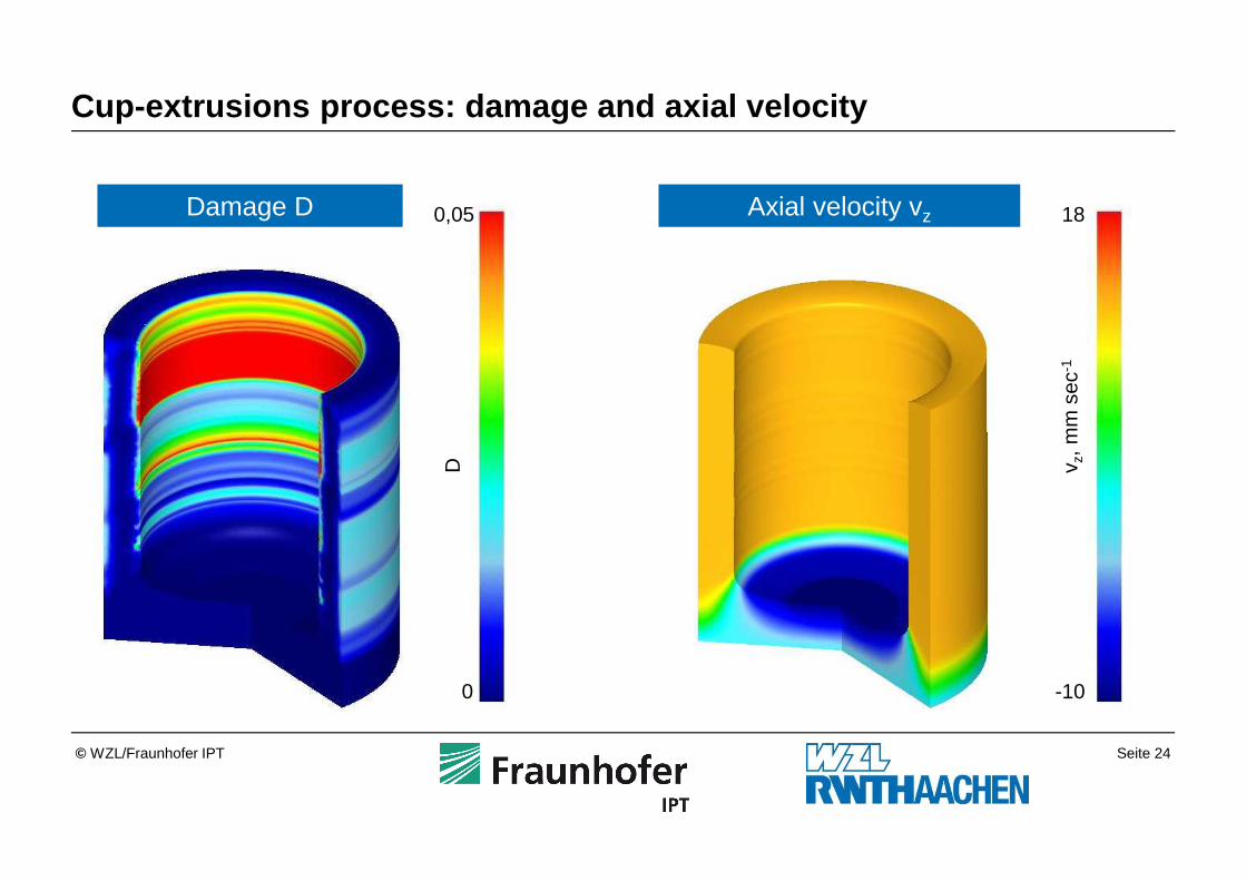
Cup-extrusions process: damage and axial velocity

1.0

0.2

0.6

0.8

Damage D

0

0,05

v z, m

m s

ec-1

Axial velocity vz

-10

18

D


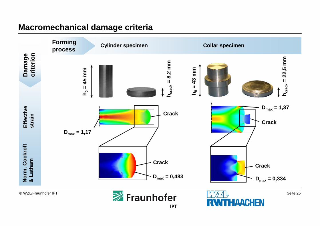
Dmax = 1,17

Crack

Dmax = 0,483

Crack

Crack

Dmax = 0,334

Crack

Effe

ctiv

e st

rain

Nor

m. C

ockr

oft

& L

atha

m

Cylinder specimen Collar specimen

Dam

age

crite

rion

Dmax = 1,37

Macromechanical damage criteria

h0

= 45

mm

h0

= 43

mm

hcr

ack

= 8,

2 m

m

hcr

ack

= 22

,5 m

m

Formingprocess


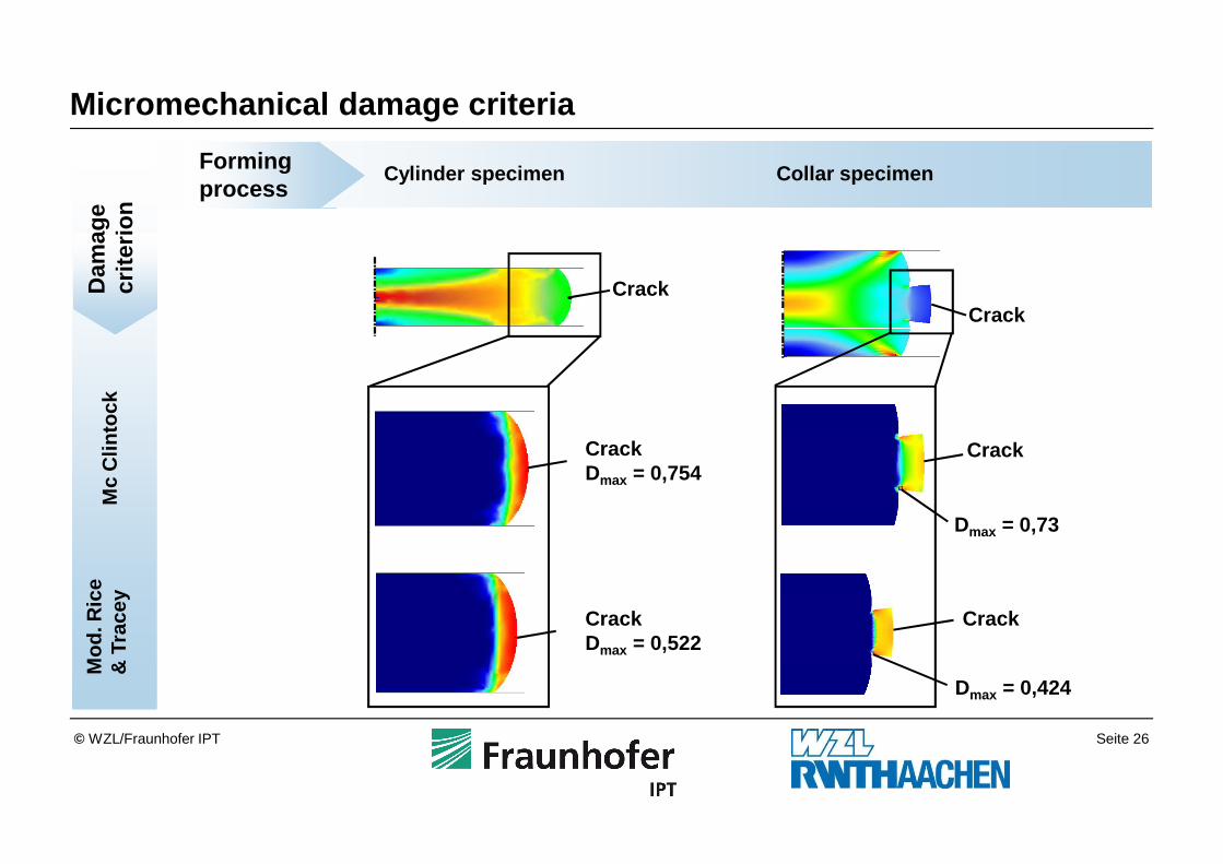
Dmax = 0,424

Mc

Clin

tock

Mod

. Ric

e &

Tra

cey

Micromechanical damage criteria

CrackDmax = 0,754

CrackDmax = 0,522

Dmax = 0,73

Dam

age

crite

rion

Cylinder specimen Collar specimenFormingprocess

CrackCrack

Crack

Crack


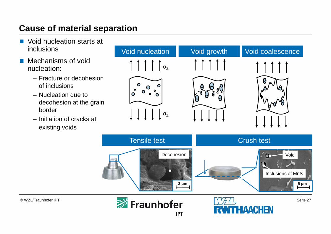
Cause of material separation

3 µm 5 µm

Tensile test Crush test

Inclusions of MnS

Void

σZ

σZ

Void growth� Void nucleation starts at

inclusions

� Mechanisms of void nucleation:

– Fracture or decohesion of inclusions

– Nucleation due to decohesion at the grain border

– Initiation of cracks at existing voids

Decohesion

Void nucleation Void coalescence


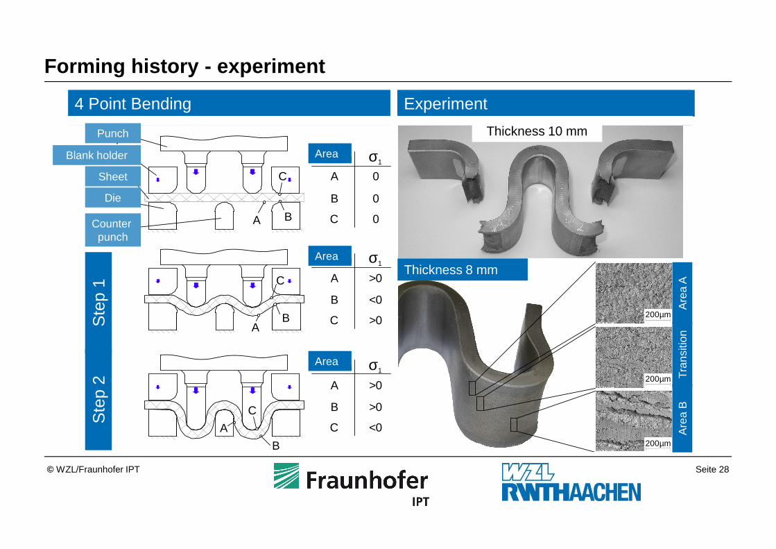
Forming history - experiment

Blech

Matrize

Stempel

Niederhalter

Gegen-stempel

A B

C

AB

C

A

B

C

σ1Bereich

A

B

C

0

0

0

4 Punkt Biegeversuch mit Umstülpung Versuchsergebnis se

Ber

eich

AB

erei

ch B

Übe

rgan

g

Blechdicke 8mm

200µm

200µm

200µm

Blechdicke 10mm

σ1Bereich

A

B

C

>0

<0

>0

σ1Bereich

A

B

C

>0

>0

<0

Pha

se 1

(1. U

mfo

rmun

g)P

hase

2(2

. Um

form

ung)

4 Point Bending Experiment

Thickness 8 mm

Are

a A

Tra

nsiti

onA

rea

B

Area

Area

Area

Punch

Counter punch

Die

Sheet

Blank holder

Ste

p 1

Ste

p 2

Thickness 10 mm


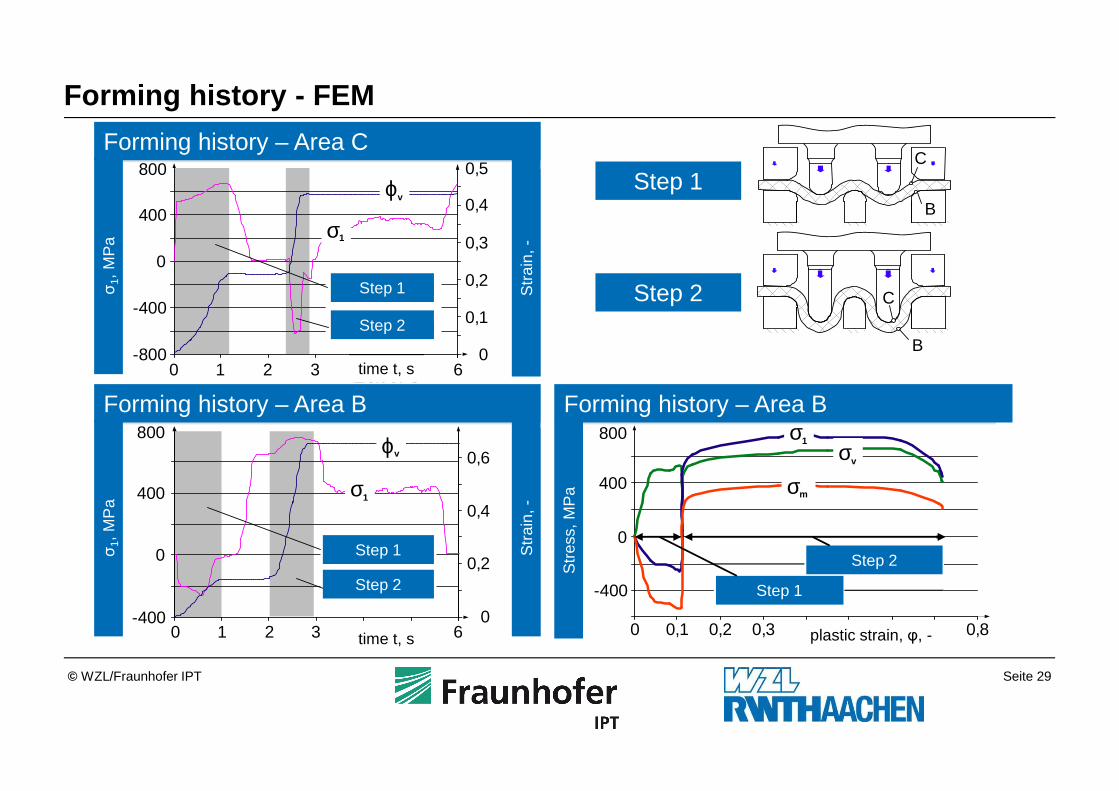
Forming history - FEM

1. UmformungB

C

2. Umformung

B

C

0

400

Umformgrad / -ϕv

Spa

nnun

g / M

Pa

0 0,1 0,2 0,3 0,8

400

800

0 1 2 3 60

0,1

0,2

0,3

0,4

0,5

-800

-400

0

Um

form

grad

/

-ϕ v

Spa

nnun

g /

MP

aσ 1

Zeit t / s

σ1

ϕv

1. Umformung

2. Umformung

-400

σv

σm

σ1

Umformgeschichte - Bereich B

1. Umformung

2. Umformung

-400

0

400

800

0 1 2 3 60

0,2

0,4

0,6

Um

form

grad

/

-ϕ v

Spa

nnun

g /

MP

aσ 1

Zeit t / s

σ1

ϕv

1. Umformung

2. Umformung

800

zeitlicher Verlauf von und - Bereich Bσ ϕ1 v

zeitlicher Verlauf von und - Bereich Cσ ϕ1 v

Step 1

Step 2

Forming history – Area C

Forming history – Area B Forming history – Area B

σ1,

MP

a

Str

ess,

MP

a

Str

ain,

-

σ1,

MP

a

Str

ain,

-

Step 1

Step 2

Step 2

Step 1

Step 1

Step 2

time t, s

time t, s

plastic strain, φ, -


Summary5


Examples3



Outline


Examples FEM -3D

Geared shaft Fender Joint


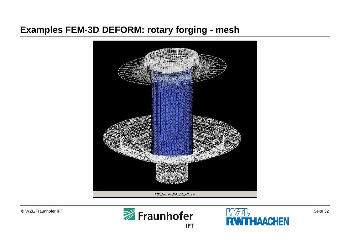
Examples FEM -3D DEFORM: rotary forging - mesh


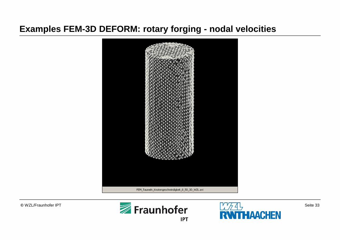
Examples FEM -3D DEFORM: rotary forging - nodal velocities


Examples FEM -3D DEFORM: rotary forging - strain


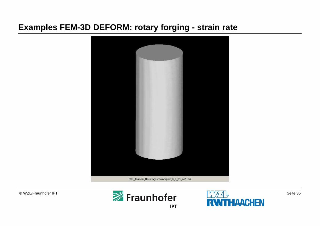
Examples FEM -3D DEFORM: rotary forging - strain rate


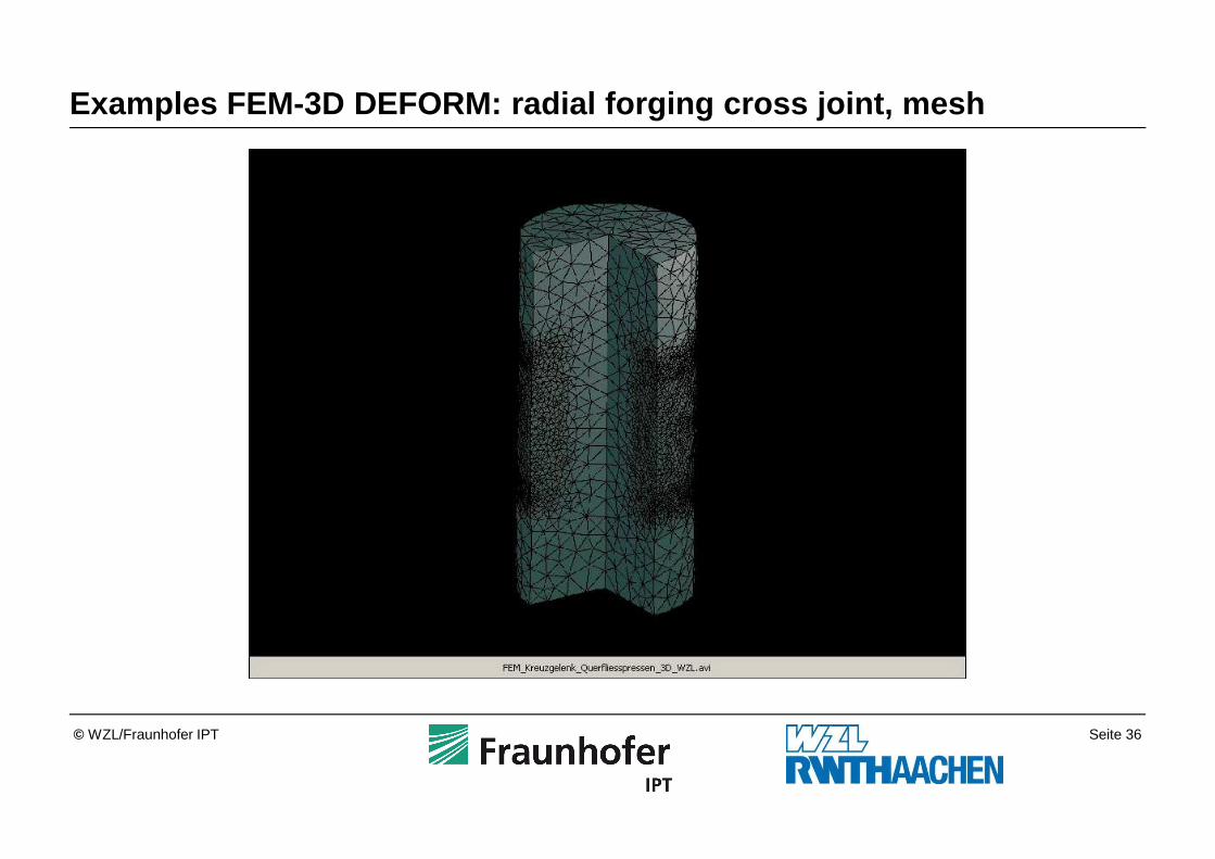
Examples FEM -3D DEFORM: radial forging cross joint, mesh


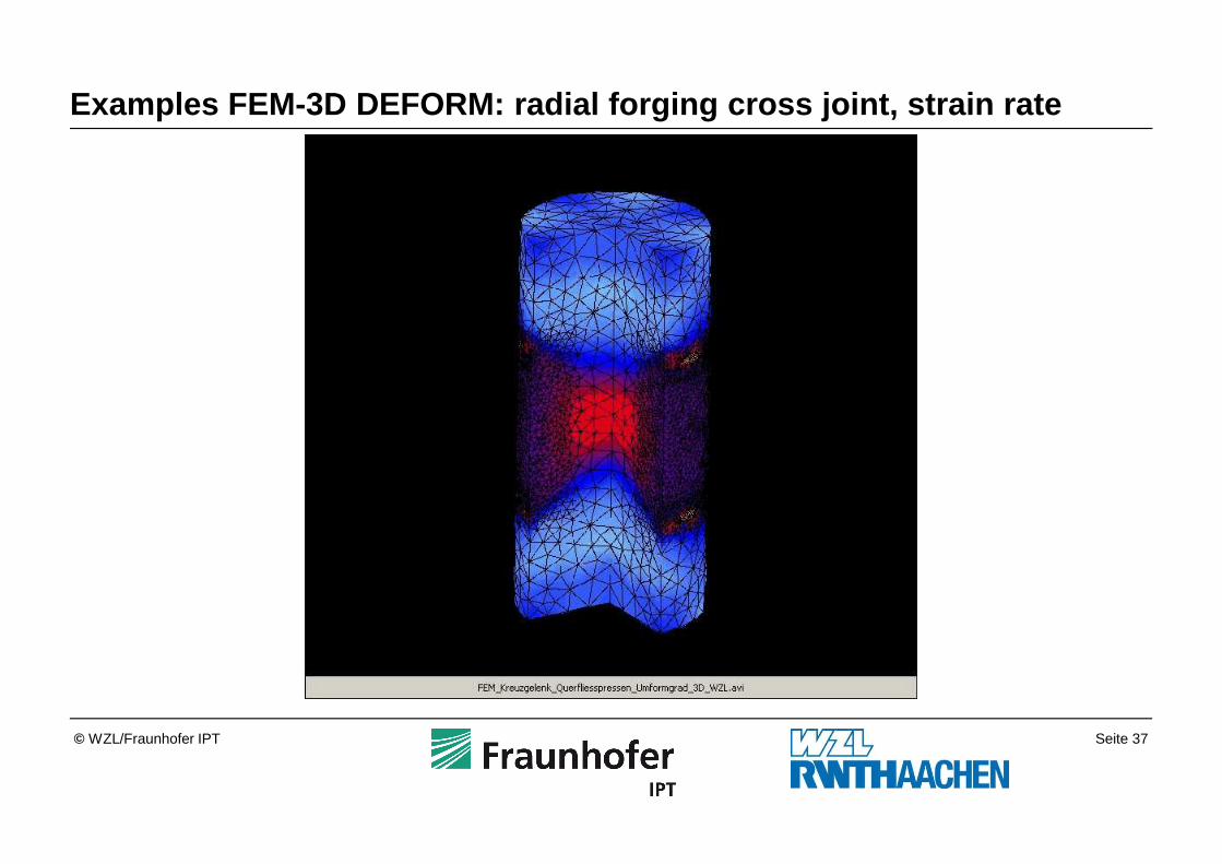
Examples FEM -3D DEFORM: radial forging cross joint, strain rate


Examples FEM -3D ABAQUS: rolling of a slab

equivalent stress

plastic strain

temperature

Source: LSTC


Summary5


Examples3



Outline


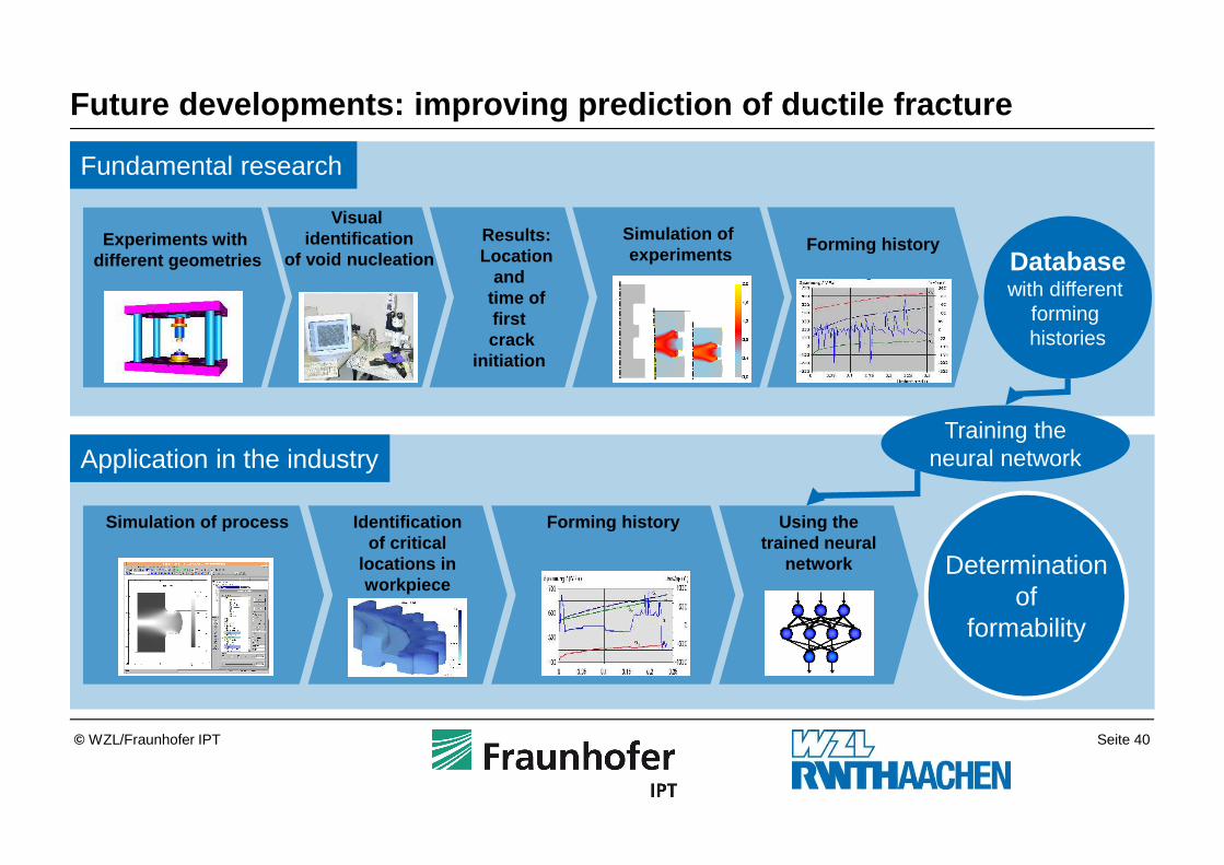
Future developments: improving prediction of ductil e fracture

Fundamental research

Results:Location

and time of first crack

initiation

Application in the industry

Forming history

Training theneural network

Databasewith different

forming histories

Simulation of process Identification of critical

locations in workpiece

Forming history Using the trained neural

network Determinationof

formability

Visual identification

of void nucleationSimulation of experiments

Experiments with different geometries


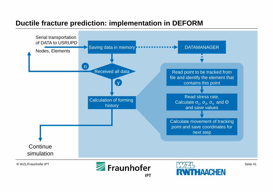
Ductile fracture prediction: implementation in DEFO RM

Saving data in memory

Calculation of forming history

DATAMANAGER

Read point to be tracked from file and identify the element that

contains this point

Read stress rate,Calculate σ1, σ3, σV and Θ

and save values

Calculate movement of tracking point and save coordinates for

next step

Continue simulation

Received all data

Serial transportation of DATA to USRUPD

Nodes, Elements

y

n


Artificial neural networks: test for formability

Analogue experiments: Compression

Other analogue experiments

Fine blanking BendingTensile testLateral extrusionIndentation test


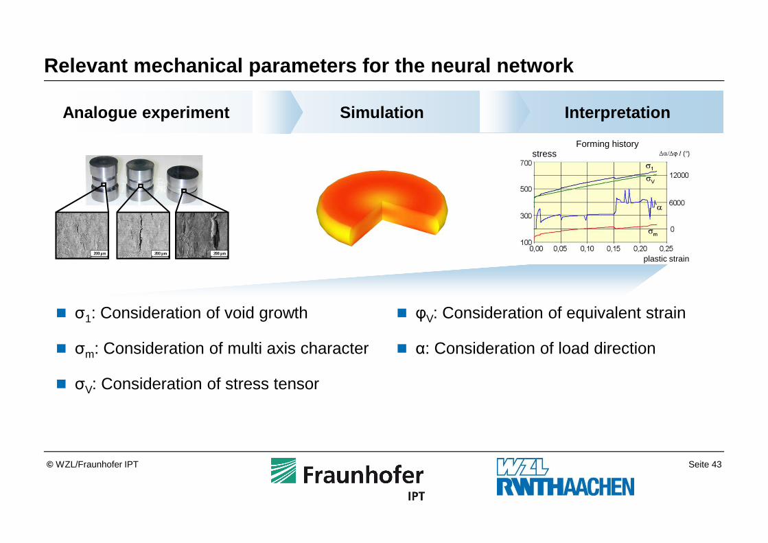
Analogue experiment Simulation Interpretation

� σ1: Consideration of void growth

� σm: Consideration of multi axis character

� σV: Consideration of stress tensor

� φV: Consideration of equivalent strain

� α: Consideration of load direction

Relevant mechanical parameters for the neural netwo rk

stressForming history

plastic strain


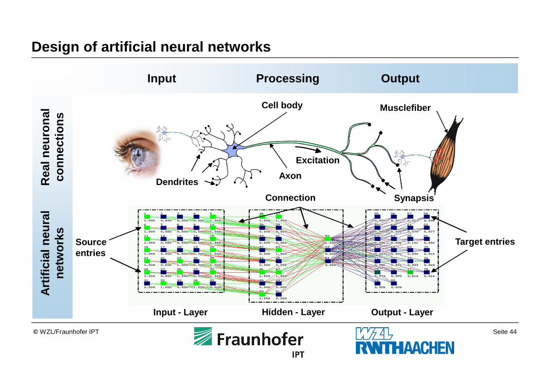
Input - Layer Output - LayerHidden - Layer

Target entriesSource entries

Connection

Axon

Cell body

Excitation

Synapsis

Musclefiber

Rea

l neu

rona

lco

nnec

tions

Art

ifici

al n

eura

lne

twor

ks

Input OutputProcessing

Dendrites

Design of artificial neural networks


DANN: Damage parameter ANN

DC&L: Damage parameter Cockroft & Latham

Damage < 100 % Damage > 100 %

Artificial neural networks: damage prediction

DANN


Future developments: Problem orientated metal formi ng simulation

� Geometry

� Material properties

� Interface conditions

� Simulation control

� Meshing parameters

� Material model

� Forces

� Velocity fields

� Strains

� Strain rates

� Stresses

� Temperatures

� Initial rod diameter

� Final rod diameter

� Workpiece and extrusion length

� Geometry of die– Standard die– Free geometry

� Punch velocity

� Material

� Does the die break?

� Does ductile fracture appear?

� Is annealing needed for recrystaization?

� Does the process work?

� How can I improve the process?

Current statusSimulation tools of

the future

Simulation input Simulation output Problem Question to answer


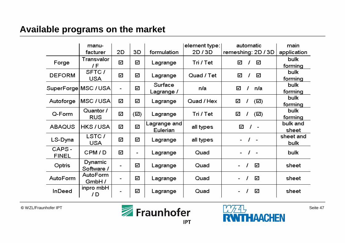
Available programs on the market


Summary5


Examples3



Outline


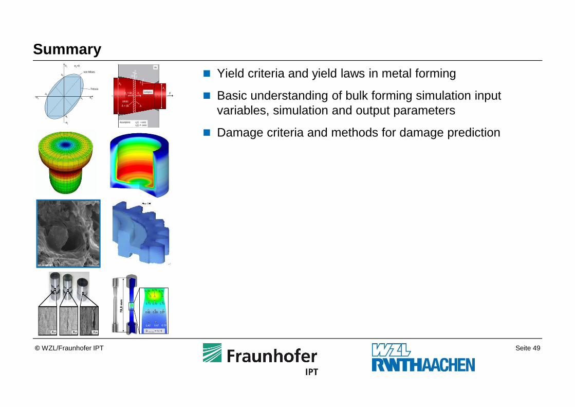
Summary

� Yield criteria and yield laws in metal forming

� Basic understanding of bulk forming simulation input variables, simulation and output parameters

� Damage criteria and methods for damage prediction

kf

-kf

σ3-σ3

σ1

-σ1

kf

-kf

σ2=0

von Mises

Tresca

A0

A1

AA + dAareas:

Fσzσz + dσz

α

pµ p

α

Assumptions: vz(r) = const.vz(z) ≠ const.

die

workpiece


Questions

� Outline the Mohr`s stress circles with uni-, bi- and triaxial compressive stress conditions.

� Explain the differences between the yield criterion of von Mises and Tresca.

� Why are the two conventional friction models (shear and coulomb) not accurate enough for the description of forging processes?

� What are typical results of a bulk forming simulation?

� Explain the approach to damage and crack prediction?

bulk metal forming ii - rwth aachen university metal forming ii simulation techniques in...

Documents