building a robust facial recognition system based … · building a robust facial recognition...

Building a Robust Facial RecognitionSystem Based on Generic Tools

Submitted in partial fulfilment

of the requirements of the degree of

Bachelor of Science (Honours)

of Rhodes University

David Pilkington

Grahamstown, South Africa

November 7, 2011

Abstract

Many software packages offer tools for image processing, manipulation, and recognition.

These tools are designed for the recognition of general images and this design for generic

recognition has various weaknesses. When considering the use of these generic tools in

the design of facial recognition system, these weaknesses may limit the robustness of the

system. These weakness include the negative effect background noise has on the recog-

nition rate, as well as the negative effect that variable lighting has on the systems per-

formance.The introduction of preprocessing improves the systems performance, especially

on images with noisy backgrounds, therefore resulting in a more robust system.

ACM Computing Classification System Classification

Thesis classification under the ACM Computing Classification System (1998 version, valid

through 2011):

I.4.8[Scene Analysis]: Object recognition

I.4.6[Segmentation]: Pixel classification

G.1.2[Numerical Linear Algebra]: Eigenvalues and eigenvectors (direct and iterative

methods)

I.5.4[Applications]: Computer Vision

Acknowledgements

I would like to acknowledge the financial and technical support of Telkom, Tellabs,

Stortech, Eastel, Bright Ideas Project 39, and THRIP through the Telkom Centre of

Excellence in the Department of Computer Science at Rhodes University.

I would also like to thank James Connan for the help, support, and guidance offered

during the course of this year. Thank you for the many meetings discussing not only

project related work, but also work currently being done in other fields, peeking my

interests and broadening my horizons.

Thank you to all my family and friends for the constant encouragement offered throughout

the year, and especially to my parents who have never stopped believing in me.

And finally, a special thank you to Kelsey Harvey for the love and support offered through-

out the year. Without the constant encouragement offered by you, this document and

year would never have been completed.

Contents

1 Introduction 5

1.1 Background and Motivation . . . . . . . . . . . . . . . . . . . . . . . . . . 5

1.2 Research Problem . . . . . . . . . . . . . . . . . . . . . . . . . . . . . . . . 6

1.3 Methodology . . . . . . . . . . . . . . . . . . . . . . . . . . . . . . . . . . 6

1.4 Goals . . . . . . . . . . . . . . . . . . . . . . . . . . . . . . . . . . . . . . . 6

1.5 Document Layout . . . . . . . . . . . . . . . . . . . . . . . . . . . . . . . . 7

2 Related Works 8

2.1 Introduction . . . . . . . . . . . . . . . . . . . . . . . . . . . . . . . . . . . 8

2.2 Facial Detection . . . . . . . . . . . . . . . . . . . . . . . . . . . . . . . . . 9

2.2.1 Attentional Cascade . . . . . . . . . . . . . . . . . . . . . . . . . . 9

2.2.2 Statistical Models . . . . . . . . . . . . . . . . . . . . . . . . . . . . 11

2.3 Facial Recognition . . . . . . . . . . . . . . . . . . . . . . . . . . . . . . . 13

2.3.1 Principle Component Analysis . . . . . . . . . . . . . . . . . . . . . 13

2.3.2 Machine Learning . . . . . . . . . . . . . . . . . . . . . . . . . . . . 16

2.3.3 Hybrid Systems . . . . . . . . . . . . . . . . . . . . . . . . . . . . . 18

2.4 Image Processing . . . . . . . . . . . . . . . . . . . . . . . . . . . . . . . . 19

2.4.1 Segmentation . . . . . . . . . . . . . . . . . . . . . . . . . . . . . . 19

2.5 Chapter Summary . . . . . . . . . . . . . . . . . . . . . . . . . . . . . . . 22

3 Benchmark System 24

3.1 Introduction . . . . . . . . . . . . . . . . . . . . . . . . . . . . . . . . . . . 24

3.2 Design . . . . . . . . . . . . . . . . . . . . . . . . . . . . . . . . . . . . . . 24

3.2.1 Image Database . . . . . . . . . . . . . . . . . . . . . . . . . . . . . 25

3.2.2 Testing Framework . . . . . . . . . . . . . . . . . . . . . . . . . . . 25

3.3 Implementation . . . . . . . . . . . . . . . . . . . . . . . . . . . . . . . . . 26

3.4 Benchmarking . . . . . . . . . . . . . . . . . . . . . . . . . . . . . . . . . . 27

3.4.1 Hardware Specifications . . . . . . . . . . . . . . . . . . . . . . . . 27

1

CONTENTS 2

3.4.2 Benchmark Results . . . . . . . . . . . . . . . . . . . . . . . . . . . 27

3.4.3 Analysis of Results . . . . . . . . . . . . . . . . . . . . . . . . . . . 28

3.5 Identified Weaknesses . . . . . . . . . . . . . . . . . . . . . . . . . . . . . . 28

3.6 Proposed Solutions . . . . . . . . . . . . . . . . . . . . . . . . . . . . . . . 29

3.7 Chapter Summary . . . . . . . . . . . . . . . . . . . . . . . . . . . . . . . 30

4 System Design and Implementation 32

4.1 Introduction . . . . . . . . . . . . . . . . . . . . . . . . . . . . . . . . . . . 32

4.2 Overall System Design . . . . . . . . . . . . . . . . . . . . . . . . . . . . . 33

4.3 Face Detector . . . . . . . . . . . . . . . . . . . . . . . . . . . . . . . . . . 33

4.4 Skin Segmentation . . . . . . . . . . . . . . . . . . . . . . . . . . . . . . . 36

4.4.1 Histogram Object . . . . . . . . . . . . . . . . . . . . . . . . . . . . 37

4.4.2 Skin Modeling . . . . . . . . . . . . . . . . . . . . . . . . . . . . . . 38

4.4.3 Segmentation . . . . . . . . . . . . . . . . . . . . . . . . . . . . . . 40

4.5 Face Recogniser . . . . . . . . . . . . . . . . . . . . . . . . . . . . . . . . . 41

4.5.1 Principle Component Analysis . . . . . . . . . . . . . . . . . . . . . 41

4.5.2 Projection . . . . . . . . . . . . . . . . . . . . . . . . . . . . . . . . 42

4.5.3 Recognition . . . . . . . . . . . . . . . . . . . . . . . . . . . . . . . 42

4.6 Chapter Summary . . . . . . . . . . . . . . . . . . . . . . . . . . . . . . . 44

5 Experimental Design and Results 45

5.1 Introduction . . . . . . . . . . . . . . . . . . . . . . . . . . . . . . . . . . . 45

5.2 Design . . . . . . . . . . . . . . . . . . . . . . . . . . . . . . . . . . . . . . 45

5.3 Results . . . . . . . . . . . . . . . . . . . . . . . . . . . . . . . . . . . . . . 46

5.4 Analysis of Results . . . . . . . . . . . . . . . . . . . . . . . . . . . . . . . 48

5.5 Chapter Summary . . . . . . . . . . . . . . . . . . . . . . . . . . . . . . . 52

6 Conclusion 53

6.1 Possible Future Work . . . . . . . . . . . . . . . . . . . . . . . . . . . . . . 54

A Glossary 59

List of Figures

2.1 Rectangles reflecting the integral images . . . . . . . . . . . . . . . . . . . 10

2.2 Viola-Jones - Identified Faces . . . . . . . . . . . . . . . . . . . . . . . . . 10

2.3 Viola-Jones - ROC Curve for the Face Detector . . . . . . . . . . . . . . . 11

2.4 Eigenfaces - Test Results . . . . . . . . . . . . . . . . . . . . . . . . . . . . 15

2.5 Artificial Neural Network - Test Results . . . . . . . . . . . . . . . . . . . 17

2.6 Logic Flow of the Hybrid System . . . . . . . . . . . . . . . . . . . . . . . 18

2.7 Comparison of Acceptance Ratio and Execution Time . . . . . . . . . . . . 19

2.8 Colour Space Comparison . . . . . . . . . . . . . . . . . . . . . . . . . . . 21

4.1 Overall system design in flow chart form . . . . . . . . . . . . . . . . . . . 33

4.2 Face Detector Demonstration . . . . . . . . . . . . . . . . . . . . . . . . . 34

4.3 Face Detection Algorithm . . . . . . . . . . . . . . . . . . . . . . . . . . . 35

4.4 Face Detection Process . . . . . . . . . . . . . . . . . . . . . . . . . . . . . 35

4.5 Nose Detection Algorithm . . . . . . . . . . . . . . . . . . . . . . . . . . . 36

4.6 Nose Detection Process . . . . . . . . . . . . . . . . . . . . . . . . . . . . . 36

4.7 Colour Space Selection . . . . . . . . . . . . . . . . . . . . . . . . . . . . . 38

4.8 RGB Histograms . . . . . . . . . . . . . . . . . . . . . . . . . . . . . . . . 38

4.9 Segmentation . . . . . . . . . . . . . . . . . . . . . . . . . . . . . . . . . . 40

4.10 Recogniser Training Algorithm . . . . . . . . . . . . . . . . . . . . . . . . . 41

4.11 Finding the Nearest Neighbor . . . . . . . . . . . . . . . . . . . . . . . . . 43

5.1 Threshold Testing . . . . . . . . . . . . . . . . . . . . . . . . . . . . . . . . 47

5.2 Euclidean Distance Comparison . . . . . . . . . . . . . . . . . . . . . . . . 49

5.3 Average Image Comparison . . . . . . . . . . . . . . . . . . . . . . . . . . 50

5.4 Timing Comparison . . . . . . . . . . . . . . . . . . . . . . . . . . . . . . . 51

6.1 Movement of the Bounding Box . . . . . . . . . . . . . . . . . . . . . . . . 55

3

List of Tables

3.1 Test Descriptions . . . . . . . . . . . . . . . . . . . . . . . . . . . . . . . . 26

3.2 Subject Descriptions . . . . . . . . . . . . . . . . . . . . . . . . . . . . . . 26

3.3 Benchmark Test Results . . . . . . . . . . . . . . . . . . . . . . . . . . . . 28

5.1 Framework 2 Description . . . . . . . . . . . . . . . . . . . . . . . . . . . . 46

5.2 Robust System Basic Test Results . . . . . . . . . . . . . . . . . . . . . . . 46

5.3 Framework 2 Test Results . . . . . . . . . . . . . . . . . . . . . . . . . . . 47

5.4 Subject Analysis . . . . . . . . . . . . . . . . . . . . . . . . . . . . . . . . 47

4

Chapter 1

Introduction

1.1 Background and Motivation

Th face is the primary focus of attention in modern society and play a significant role

in an individuals identity [13]. The human ability for facial recognition is remarkably

robust as despite of the large changes in viewing conditions, the human mind is able to

recognise thousands of faces [13]. Thus, in todays technological world, attempts are being

made to transfer this ability to computer systems. These systems can be used in a large

variety of manners such as criminal identification, security systems and human-computer

interactions [13]. However, this presents problems do to the complex, multidimensional

nature of the human face [13]. And thus, tools need to be used to reduce the noise within

the images so that a more robust face recognition can be implemented [13].

There exist multiple packages that offer tools that can be used to implement computer

vision systems. These packages provide many generic tools that can be used for various

image processing and manipulation tasks. While these tools may offer many uses to many

users, those that wish to use them for a robust facial recognition system may find the

tools ill-suited to some aspects of the system. The reason for this is due to the inherent

generic nature of the tools as they are not tailored specifically to the needs of a facial

recognition system.

One such package is EmguCV. This is a C# wrapper for the OpenCV package which is

in C++. This package offer the EigenObjectRecognizer as a generic image recogniser and

this will be used in the research that follows.

5

1.2. RESEARCH PROBLEM 6

1.2 Research Problem

The tools provided by the packages mentioned above do not always produce a system

that can recognise faces in varying conditions and thus the following research question is

posed: What effects will preprocessing have on a system built on generic tools?

To answer this, the following questions must first be answered.

• What is the performance of the generic recognition tool?

• What points of weaknesses can be identified with the tool?

• How can these weakness be used to develop a system that proves to be more robust

than the generic tools?

1.3 Methodology

To determine whether the system proposed and developed in this document is in fact more

robust than the generic tools provided by the package, two systems will be developed and

their performances will be compared.

These two systems will consist of:

• A benchmark system that consists only of the generic tools provided by the package

for image recognition.

• Weakness are identified within the benchmark system.

• A system whose components have been designed and developed to compensate for

weaknesses identified from the testing of the benchmark system mentioned above.

Both of these systems will undergo a similar testing framework to compare performance.

The developed system will also undergo additional tests to identify potential improvements

that can be made in future work in order to improve the robustness of the system.

1.4 Goals

The goal of this thesis is to develop a facial recognition system that is robust in nature.

This implies that it has the following characteristics:

1.5. DOCUMENT LAYOUT 7

• The system should be able to identify faces even with varying amounts of background

noise.

• The system should be able to achieve a high rate of positive recognition.

• The system should be able to reject an individual not within the training set yet

have low rates of false rejects where an individual within the system is wrongly

rejected.

• The system should not be highly susceptible to the changing of lighting conditions

within the image.

1.5 Document Layout

Chapter Two contains a review of the literature that covers work related to the field being

researched and thus provided a theoretical background against which this thesis is based.

Chapter Three contains the design and implementation of the benchmark system that is

built only of the generic tools provided by the EmguCV package for image recognition.

The testing and results thereof are also discussed. From these results, weaknesses of the

system are identified and possible solutions proposed.

Chapter Four discusses the design and implementation of the developed system. The

overall design of the system as well as the design and implementation of each individual

component is discussed.

Chapter Five reviews the performance of the system based on the testing frameworks

described. These results are then analysed and compared against those of the benchmark

system obtained in Chapter Three. More detailed testing is also done on the developed

system.

Chapter Six concludes the thesis and makes suggestions for possible extensions that can

possible lead to the system being even more robust.

Chapter 2

Related Works

2.1 Introduction

The field of Biometric Identification involves the use of physiological and behavioural

characteristics to uniquely identify a particular individual [8]. These methods vary in

invasiveness. From the most extreme case of DNA testing, to the less invasive finger/hand

printing, to the least invasive of all, facial recognition.

It is this least invasive technique (that of facial recognition) that will be the main focus of

this review. All other forms of biometric identification fall out of the scope of this review

and thus will be overlooked.

The main challenge in the field of facial recognition is that of variable input. This means

that the input provided to the system is never the same as the test cases maintained

within the database. This variability is caused by illumination variability, facial features

and expressions, and occlusions, etc [11].

When considering the field of facial recognition, in terms of biometric access control, one

notices that the system used for the biometric identification of an individual has three

components, those being: Facial Detection, Facial Recognition, and Image Processing [8].

The facial detection component is responsible for the identification of possible faces within

the provided image. The facial recognition component is then responsible for the compar-

ison of the previously identified faces against a pre-existing image database in an attempt

to identify the individual in the image. Finally, the image processing component is the

most pervasive of all as it is called by all other components to process the image to

8

2.2. FACIAL DETECTION 9

transform it into a state that is most suitable for the respective component[8].

Each of these fields have a variety for algorithms that have been developed to suite

varying contexts. The more appropriate algorithms (with regards to biometric access

control systems) will be reviewed according to their strengths and weakness with regards

to the algorithm itself, as well as the algorithms compatibility with other components.

2.2 Facial Detection

Facial detection refers to the identification of faces within the specific image. This serves

to reduce the surface area of the image to aid the process of recognition[6]. Only the

face of the individual is then passed to the face recognising component so as to reduce

the background noise that may interfere in the recognition process. This poses a problem

as the human face has been described as ’a dynamic object and has a high degree of

variability’[6].

2.2.1 Attentional Cascade

The attentional cascade is one of the algorithms that has shown the most promising

results for the detection of faces within real-time video [15]. One of the most prominent

implementations of this algorithm was developed by Viola and Jones.

Representations

Viola and Jones developed a new representation of the image for use in their face detection

algorithm, it was called the ’Integral Image’ [15].

The rectangle features of the image can be computed rapidly with the use of the integral

image as an intermediate representation [15]. The integral image at the location x, y

contains the sum of the pixels above and to the left of the x and y coordinates[15] and

can be represented by the formula below:

ii(x, y) =∑

x′≤x,y′≤y

i(x′, y′) (2.1)

A graphical representation of the integral image can be seen below:


Figure 2.1: Rectangles reflecting the integral images

In the above figure, the value of the integral image at point 1 can be calculated by summing

the pixels within the rectangle A. The integral image at point 3 would be the sum of the

pixels in rectangles A and C. The integral image at point 4 would thus be equal to the

sum of the 4 rectangles A, B, C, and D [15]

Learning Classifications

Many of the machine learning approaches make use of a training set of both positive and

negative examples[15]. The algorithm used in [15] is that of AdaBoost. It has been stated

that generalisation performance is directly related to the margin of examples, and thus

AdaBoost is suited to this as it achieves large margins rapidly [15].

These classifiers are then organised in a cascade to increase the detection performance as

well as reducing the required computation time dramatically [15]. The basic algorithm

behind this approach is that simpler classifiers reject the majority of the image. The more

complex classifiers are then called upon to reduce the rate of false positives posed by the

simpler and less discriminatory classifiers [15].

Results Obtained

Below are the outputs of the system developed in [15].

Figure 2.2: Viola-Jones - Identified Faces


From this image, we can see that the detector has able to detect multiple faces within an

input image.

From the testing conducted in [15], the following results were obtained:

Figure 2.3: Viola-Jones - ROC Curve for the Face Detector

Here we can see how the detector generates an almost 95% correct detection rate [15]

showing the accuracy of the system to be high.

Advantages

As mentioned above, the cascading classifier algorithm produces highly efficient detection

results. When compared to other detection algorithms, the attentional cascade required

only 0.7 seconds to scan a 384 x 288 image, the fastest of any published facial detection

system[15].

Disadvantages

During the construction of the cascade of classifiers, more and more discriminatory classi-

fiers are needed that offer higher detection rates and lower false positive rates. The more

specific the classifier, the more features it has and thus requires more time to compute[15].

2.2.2 Statistical Models

There are several statistical approaches to face detection.These include, but are not limited

to, information theory, a support vector machine, and the Bayesian Decision Rule[6].


Calmenarez and Huang proposed a system that was fundamentally based on Kullback

relative information/divergence[6]. This was a nonnegative measure of the difference

between the two probability density functions P nX and Mn

X where Xn was a random

process[6]. A join histogram was used to create the probability functions of the classes

for positive faces and negative face examples. The value of a pixel is largely dependent on

the value of the adjacent pixels and thus Xn is treated as a first order Markov process[6].

Another system was proposed by Schneiderman and Kanade where the probability func-

tion is derived based on a set of operations, modifications, and simplifications to the

image[6]. These can be seen below[6]:

• The image resolution of the face image is normalised to 64x64

• The face images are then decomposed into 16x16 subregions.

• The subregions are then projected onto a 12-dimensional subspace, constructed with

the use of Principal Component Analysis.

• The entire face region is then normalised to have zero mean and unitary variance.

Advantages

All of the systems tested in [6] show high correct detections within the varying image

databases used. This shows that the usefulness of this approach, that of statistics, is

pervasive as it has encouraging results in many different test cases.

Disadvantages

While the systems should a good correct detection dimension to the testing, many of

them (most notably Colmenarez and Huang) proved to have a high false positive rate [6]

and this can prove detrimental in the case of real time Facial Recognition System where

efficiency is key.

[6] also states that the feature based statistical systems can almost only be exclusively

used in real time systems as they require colour information as well as motion in some

cases.

2.3. FACIAL RECOGNITION 13

2.3 Facial Recognition

Once the face has been detected by the facial detection component of the system, it must

then be compared to a database of known personnel to confirm the identity. The two

main approaches reviewed here are that of Principle Component Analysis as well as that

of Machine Learning.

2.3.1 Principle Component Analysis

The method of Principle Component Analysis (PCA) moves away from the use of natural

bases to that of orthonormal basis [8]. It is a mathematical procedure whose aim is to

transform a number of possibly correlated variables into a smaller number of uncorrelated

variables called principle components [13].

An example of this basis is Karhonen-Loeve (KL) where the KL bases are made up of

eigenvectors of the covariance matrix of the face, KL bases are thusly also known as

eigenfaces [8]. Due to the nature of PCA, any face can be represented along the eigen

pictures coordinate space as well as being reconstructed using a portion of the eigen

pictures[13].

Principle Component Analysis Algorithm

The PCA algorithm is as follows [13]:

1. Obtain the initial training set of M faces and then calculate the eigenfaces from this

set. Only the set of eigenfaces (M’ ) that correspond to the highest eigenvalue are

kept.

2. Calculate the corresponding distribution in M’ -dimensional weight space for each

known individual, and then calculate a set of weights based on the input image.

3. Classify the weight pattern as either a known or unknown individual according to

the Euclidean Distance to the closest weight vector of a known person.

The calculation of the average face is seen below, where M represents the number of

images within the training set and with Γ representing an image from the training set.


Ψ =1

M

M∑n=1

Γn (2.2)

Thus once the average face has been calculated, we can see how each individual face differs

from the average with the following vector:

Φi = Γi −Ψ (2.3)

This is then calculated for each of the images in the training set and the co-variance

matrix is formed in the fashion shown above.

C =1

M

M∑n=1

Φn.ΦTn = A.AT (2.4)

Thus leading to the matrix

A = [Φ1,Φ2, ....,ΦM ] (2.5)

It is this set of vectors that is then subjected to the PCA to obtain a set of M orthonormal

vectors u1...uM . Then once the new vector have been formed, it is used in the formation

of the weight vector Ω. To obtain the Ω of contributions of the individual eigenfaces to a

particular face image, Γ , the face image undergoes a transformation into its own eigenface

components and then projects onto the face space via the following operation.

ωk = uTk (Γ−Ψ) (2.6)

These weights thus form the above-mentioned vector Ω. This represents the contribution

of each individual eigenface within the representation of Γ. Using this, one can use the

Euclidean Distance (εk) between the Ω of the input image and the Ωk (where is is an

image in the training set that is closest to Ω).

εk =‖ Ω− Ωk ‖2 (2.7)


Once εk has been calculated, it is then compared to a threshold value that is predeter-

mined. If εk is less than the threshold, it is deemed to be close enough to Γk and is

identified as such. If not, the face is not recognised.

Eigenfaces Results

The following results were presented from the testing reported in [13]:

Figure 2.4: Eigenfaces - Test Results

When testing the various variables were changed, these included lighting, orientation, and

scale.

• Graph A - Variable Lighting

• Graph B - Variable Scale

• Graph C - Variable Orientation

• Graph D - Variable Lighting and Orientation

• Graph E - Variable Scale and Orientation #1

• Graph F - Variable Scale and Orientation #2

• Graph G - Variable Scale and Lighting #1


• Graph H - Variable Scale and Lighting #2

From the above we can see that the system produces a high rate of recognition but this

rate is extremely susceptible to changes in the conditions of the images being test.

Advantages

The eigenface approach, and thus the use of PCA, has proved to be fast and relatively

simple to implement as well as working well in a constrained environment [13]. [8] states

that PCA is optimal in the sense of efficiency.

The nature of PCA also allows for modularity and thus compatibility with other methods

such as machine learning[13] which leads to the possibility of cohesive hybrid systems to

be reviewed below.

Disadvantages

While it has been stated that PCA has the optimal efficiency, it has also been stated that

it does not stand to say that it is optimal on the basis of discriminating power and thus

recognition as a whole[8]. This relies on the separation between different faces rather than

the spread of all the faces [8].

[13] also states that the eigenface technique, and thus PCA, offers an unknown rejection

rate. As most Facial Recognition Systems require a low false positive rate[13], there may

be cases where the variable rejection is not acceptable.

Finally, [13] recognises the trade-off between the number of people that the FRS needs to

recognise and the number of eigenfaces required for unambiguous recognition.

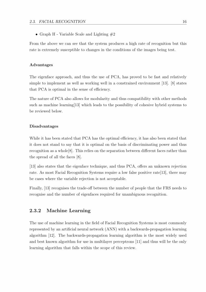
2.3.2 Machine Learning

The use of machine learning in the field of Facial Recognition Systems is most commonly

represented by an artificial neural network (ANN) with a backwards-propagation learning

algorithm [12]. The backwards-propagation learning algorithm is the most widely used

and best known algorithm for use in multilayer perceptrons [11] and thus will be the only

learning algorithm that falls within the scope of this review.


Artificial Neural Networks with a Backwards Propagation Learning Algorithm

Within the layout of the ANN, each node requires an activation function that will decide

the output of the node depending on the inputs [12]. The most commonly used activation

function identified by [12] is the log-sigmoid function. This is due to the fact that the

function outputs 1’s and 0’s and thus is suited to the use of boolean outputs[12].

As the ANN will receive input that is variable (termed ’noisy’ by [12]) the training set of

images is usually a combination of ideal and non-ideal images[12].

Results

During the testing presented in [12], the following results were presented:

Figure 2.5: Artificial Neural Network - Test Results

From the above, it can be seen that the neural network presented in [12] obtained ex-

tremely high rates of recognition. However the time taken to train the network is always

within the range of a few hours.

Advantages

ANN’s, and thus machine learning, offer a highly effective rate due to their ability to

learn[12]. In the tests conducted by [12], various ANN’s, trained using the method men-

tioned above, never achieved recognition rates of below 95 percent when they were left to

train for over 2 hours. This recognition rate is remarkable and can increase with increased

training time, until the recognition peak has been reached[12].


Disadvantages

One of major disadvantages of the use of a neural network is the required complexity.

For every pixel that constitutes part of the input image, a separate node is required in

the input layer of the ANN [8]. This means that even a relatively small input image of

128x128 pixels would require over 16 000 input nodes.

One method for combating this linearly increasing complexity is to make use of down-

sampling[11]. The method involves shrinking the image to a 20x20 facial feature vector

that will thusly only require 400 input nodes, leading to a conceptually simple ANN.

When considering the training of the ANN according to the method suggested by [12],

the ANN may become so adept at identifying the non-ideal images, that it will become

less adept as recognising the more ideal input images[12].

2.3.3 Hybrid Systems

Hybrid systems use a combination of the above techniques to compensate for the weak-

nesses of an approach with the strengths of another. An example of this can be seen by

the hybrid recognition system presented in [11]. Here, PCA is first used as a technique to

identify patterns within the data i.e. feature extraction [11]. The logic flow of the hybrid

system can be seen in Figure 2.6.

Figure 2.6: Logic Flow of the Hybrid System

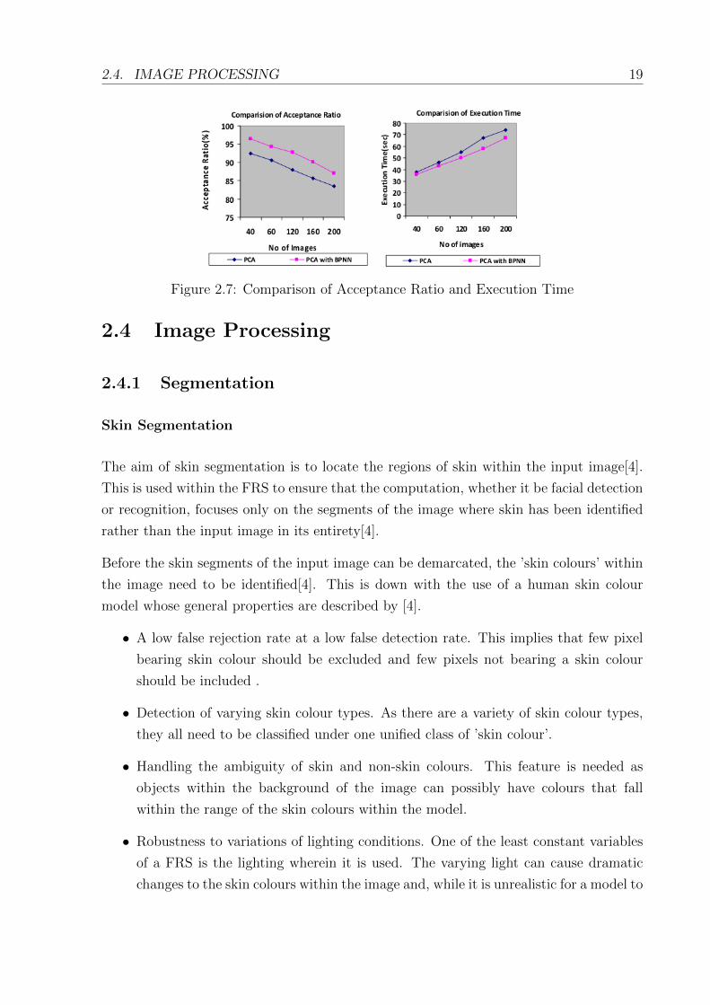
The benefits of such hybrid systems are most clearly expressed in the performance results

of the system. The system mentioned in [11] bore the results illustrated in Figure 2.7.

From this, we can see that by combining the PCA approach with the use of an ANN, the

acceptance rate not only increase, but so does the execution time, thus leading to a more

effective and efficient system

2.4. IMAGE PROCESSING 19

Figure 2.7: Comparison of Acceptance Ratio and Execution Time

2.4 Image Processing

2.4.1 Segmentation

Skin Segmentation

The aim of skin segmentation is to locate the regions of skin within the input image[4].

This is used within the FRS to ensure that the computation, whether it be facial detection

or recognition, focuses only on the segments of the image where skin has been identified

rather than the input image in its entirety[4].

Before the skin segments of the input image can be demarcated, the ’skin colours’ within

the image need to be identified[4]. This is down with the use of a human skin colour

model whose general properties are described by [4].

• A low false rejection rate at a low false detection rate. This implies that few pixel

bearing skin colour should be excluded and few pixels not bearing a skin colour

should be included .

• Detection of varying skin colour types. As there are a variety of skin colour types,

they all need to be classified under one unified class of ’skin colour’.

• Handling the ambiguity of skin and non-skin colours. This feature is needed as

objects within the background of the image can possibly have colours that fall

within the range of the skin colours within the model.

• Robustness to variations of lighting conditions. One of the least constant variables

of a FRS is the lighting wherein it is used. The varying light can cause dramatic

changes to the skin colours within the image and, while it is unrealistic for a model to


account for every possible lighting condition, the model should have some robustness

in this area.

The skin model then needs a colour space as well as a colour classification algorithm in

which to operate[4].

There are currently a vast number of classifications out these including, but not limited

to : Multilayer Perceptrons, Self-organising Maps, Linear Decision Boundaries, etc [4].

The one used in [4] that showed an increase in performance was the Bayesian decision

rule for Minimum Cost.

With regards to the various colours spaces that the model can operate in, as with the

above classification algorithms, the variety is vast [4]. The colour spaces included, but

are not limited to: RGB, YCbCr, HSV,normalised RGB, etc [4]. One of the finding of [4]

was the there was no identifiable performance difference between the colour spaces with

the colour histogram sizes greater than 128 bins per channel.

The advantages of this technique are:

• All colour channels show an increased performance over the exclusive use of chromi-

nance channels[4].

• The coupling of techniques can prove to provide a more efficient skin classification

algorithm [10]

These are, however, coupled with the following disadvantages:

• The coupling of techniques for increased efficiency can lead to the algorithm becom-

ing overly complicated and thus requiring more memory and more computational

resources[10].

• Already acknowledged by [4] is the fact that the background can contain items whose

colour falls within the skin model and this noise can present issues for recognition

techniques where noise can skew the results[8].

Results

A comparison of colour spaces is presented in [10].


Figure 2.8: Colour Space Comparison

From the above, a comparison is made concerning the different colour spaces. From this,

we can see the use of HSV and RGB produces a better rate of recognition than the others

presented thus showing why these are preferred for use in skin segmentation.

Background Subtraction

Due to the fixed location of many cameras, whose images are used as input for Facial

Recognition Systems, background subtraction (also known as background differencing) is

the most fundamental image operation for security systems[5].

Before one can begin the process of background subtraction, a ’model’ of the background

must first be learnt[5]. This model is then compared to the input image and the known

background segments are subtracted away. This model is not always sufficient however as,

due to the context of the camera, the foreground and background are flexible concepts[5].

The complication is overcome by the developing of a scene model. In this, there are

multiple levels between what is defined as the foreground and what is defined as the

background[5].

This method aids in the identification of newer object that may have been placed in

the scene but, as they are not the focus of the system, are still regarded as part of this

background. This is accomplished by placing the new object in a ’newer’ level of the

background, and, over time, it will shrink into the older levels of the model until it is part

of the original background[5].

2.5. CHAPTER SUMMARY 22

In the case of a massive environment change, global frame differencing can be used[5].

This kind of change can be identified by many pixels changing value at the same time[5].

The advantages of background subtraction are as follows:

This method makes use of the context of the camera to aid in the segmentation of the im-

age and thus does not require the statistical computation that skin segmentation does[5].

Bearing the above in mind, the follow present challenges for the use of back-

ground subtraction:

• One of the major flaws of the background subtraction technique is that it assumes

that all pixels are independent and thus only works well in simple backgrounds[5].

• By accounting for this weakness, by the use of modeling, the technique creates more

disadvantages in the form of increase memory consumption and computation[5].

This approach also requires that there be a substantial increase in the data provided

to create the more complex models[5].

2.5 Chapter Summary

As can be seen by the above literature, the field of biometric identification, and more

specifically. Facial Recognition systems.

There are varying approaches to each component that makes up the Facial Recognition

System. Those components being the detecting of the face, the recognition of the face

and the processing of the image at various points of the system. Each approach has had

its advantages juxtaposed with its disadvantages. This allows for the realisation that

the use of a specific approach is context sensitive. Factors such as required efficiency

and effectiveness, availability of computational resources, availability of memory (both

primary and secondary), the hardware used to provide the input, the format of the input,

an others need to be taken into account before choosing the correct components.

With regards to the system being developed in this project, the following techniques have

been chosen based on their relevance and and the positive aspects associated with them

that suite the context of the system.

For the facial detection component of the system, the attentional cascade will be used,

more specifically one similar to that propose and developed by [15]. This choice has the


following justifications:

• The system uses real-time video as the input for the system. As mentioned above,

the attentional cascade has proved to be the most efficient means of face detection

when computational time is a factor that needs to be minimised. The attentional

cascade has been shown to be able to have a detection rate of 15 fps (frames per

second) and this suites the context of the system.

• With regards to the weakness identified, it can be counteracted by the nature of

the system itself. The fact that the system will not need to be trained in real time

means that all classifier training can be done during the developmental stages of the

project and non has to be done while the system is in use.

The principal component analysis approach, more specifically the eigenface technique,

will be used for the recognition component. The justifications are as follows:

• The efficiency shown by the algorithm again suite the real time context of the system

and is suited to the rapid detection rates of the attentional cascade chosen above.

• The modularity of the approach allows for future expansion on the project. For more

effective recognition results, the PCA component can be combined with a machine

learning technique to create a hybrid recognition component.

Due to the latter, the approach of machine learning is not completely disregarded, but

merely kept as a possibility for future development work on the systems

Finally, with regard to the image processing component of the system, skin segmentation

will be used for the following reasons:

• The eigenface technique is more efficient with as little background noise as possible[8]

and the use of skin segmentation will allow for this noise to be minimised.

• The background subtraction is too general for use in a biometric access control sys-

tem, where security and precision is key, as the nature of the background (especially

in the location context of the system, an office area with many people moving in

and out of focus) is dynamic and thus the modeling approach offered as a solution

above, does not apply.

Chapter 3

Benchmark System

3.1 Introduction

The purpose of the benchmark system is to identify a performance baseline against which

the performance of the final system can be compared. This system will also be used to

identify the shortfalls of the generic recognition tools provided by the package. These

shortfalls will become the identified weaknesses of the system and will be used as the

foundation for the design and implementation of components that will aim to compen-

sate for these weaknesses. In this chapter, the design for the benchmark system will be

discussed along with the implementation, testing, and examination thereof.

3.2 Design

The aim of the design for the benchmark system is to rely on only the recognition compo-

nents provided by the EmguCV package. This component is known as the EigenObjec-

tRecognizer which makes use of the PCA algorithm as a means of recognition citeemguweb

. The constructor of this object takes in the following parameters:

• An array of grey scale images that are used to train the recogniser.

• An array of strings which act as the identifiers for each of the training images.

• A reference to a MCvTermCriteria which acts as the termination criteria for the

PCA algorithm used within the eigenfaces technique.

24

3.2. DESIGN 25

3.2.1 Image Database

The image database used in this research project was designed for the specific use of

testing both the benchmark system and the developed system according to the goals set

forth in Chapter 1.

The data set contains 30 images in total. These 30 images are composed of 6 images

each of 5 individuals. These images have been captured using the tools provided by the

EmguCV package so as to allow for greater consistency within the tests. These images of

the individuals have been captured and stored based on the criteria mentioned in Table

3.2.

Each image is stored as a Portable Network Graphics (PNG) [9] file with a resolution of

640 x 480 pixels and are taken and stored in RGB format. The choice of PNG is due to

the lossless compression of the file format which means that the exact image data can be

restored from the compressed data[9]. This is preferred over the use of Joint Photographic

Experts Group (JPEG)[9] files which makes use of lossy data compression. This means

that the original image data is partially lost due when the image is initially compressed.

The images were taken at separate times as to maximise the variability within the images

themselves. This results in increased variability in lighting, clothing, and facial expression.

The individuals1 chosen for the database are diverse in nature. There are representatives

from a diverse selection of skin tones. This too allows for increased variability.

3.2.2 Testing Framework

The testing framework detailed here will be used both for the testing of the benchmark

system and for the testing of the final system. This will ensure that both sets of tests will

have undergone the same procedure as to ensure the integrity of the results they produce.

The entire testing process will consist of 5 tests. The details of these tests are detailed in

Table 3.1:

1All individuals participating in this database have done so out of their own free will and have signeda consent for allowing the use of their likeness in any documentation or publication resulting from thisresearch.

3.3. IMPLEMENTATION 26

Table 3.1: Test Descriptions

Test 1 5 training images per individual




Test 5 1 training image per individual

The aim of this testing process is firstly to establish a baseline against which the perfor-

mance of the final system can be compared. But it also has the secondary function of

establishing performance gain per training image used.

For the purposes of this testing, five subjects are used each with varying degrees of

background noise in each image. The images captured for each subject have been designed

to follow the following pattern:

Table 3.2: Subject Descriptions

Subject Image Description

1 3 Different backgrounds with the images taken over 3 different days at varying times

during the day.

2 Static Background taken all at the same time

3 Taken at the same time but at varying angles of the same room

4 Taken with the same background over 2 days with people walking in the background

5 5 images with a static background and 1 image with a varied angel of the face

3.3 Implementation

The implementation of the benchmark system was implicitly simple due to the fact that

only the primary, basic, generic tools are used in the system.

First, the images are loaded from file into the system. These are stored in an array of

Image(Gray, Byte) objects as this is what the recogniser requires. While these images are

being loaded into the system, the individuals name is extracted from the file name and

simultaneously added to a string array. Once this process is complete, the EigenObjec-

tRecognizer object is created with the following parameters[3]:

3.4. BENCHMARKING 27

• An array of Image(Gray, byte) images which serves as the training data for the

recogniser.

• An array of string, the same size as the array mentioned above, with each element

being the label of the corresponding image of the training array.

• A reference to a MCvTermCriteria object which serves as the termination criteria

of the PCA algorithm used by the EigenObjectRecognizer.

When creating the recognition object, a MCvTermCriteria reference also needs to be

passed to the constructor. This value is set to 0.001. For the purposes of this benchmark

system, this is assumed as the default value as it is the value recommended on the package

website under tutorials [1].

Once this process is complete, the test images are loaded from file into the system. This

process is similar to the one mentioned for the loading of the training data. Once the

loading process has been completed, the program enters the testing framework.

Once each of the tests has been completed, the results are both outputted to the screen

and to file.

3.4 Benchmarking

3.4.1 Hardware Specifications

For the purposes of the testing, the machine that ran the testing framework had the

following hardware and software specifications:

• Intel Core 2 Quad Q6600 @2.4 GHz

• 6 Gb DDR2-800 RAM (only 3.5 Gb usable due to operating system constraints)

• Windows 7 Ultimate (32bit)

• Logitech 300 WebCam

3.4.2 Benchmark Results

Using the testing framework detailed in Table 3.1, the following results were obtained:

3.5. IDENTIFIED WEAKNESSES 28

Table 3.3: Benchmark Test Results

Test Result (recognition rate in %) Database Load Time (s)

1 40 0.3992

2 40 0.7962

3 40 1.4465

4 40 2.2438

5 40 3.3414

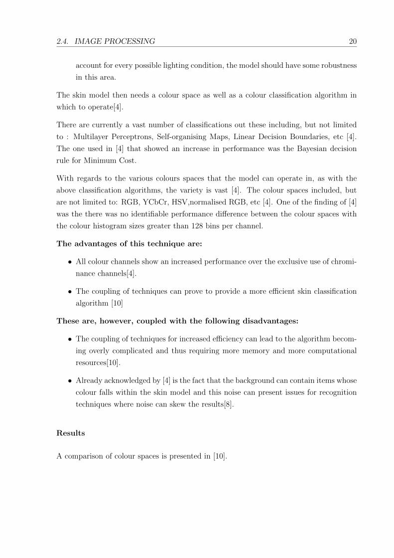
3.4.3 Analysis of Results

From the above results the following observations can be made.

First, the recognition rate is constant at 40%. This low rate is a testament to the effect

that a variable background has on the system. As the recognition technique used by the

EigenObjectRecognizer (that of eigenfaces), the background noise of the images leads to

principle components being identified within the image that do not correspond with the

face in question[13].

From these results we can see that the only correct recognitions are for subjects 2 and

3 (from Table 3.2). This means shows that the benchmark system can handle the static

backgrounds and backgrounds that are similar but, even with an increase in the amount

of training images, the changing backgrounds prove to be difficult for the recogniser to

correctly recognise.

Another observation is the fast load time from the database. This is understandable as

no image processing (besides the required grey scale conversion) is performed.

With these results and observations in mind, the weaknesses of the system can be identified

and discussed.

3.5 Identified Weaknesses

Based on the results from the benchmarking procedure above, the following observations

were made:

• The rate of recognition achieved by the EigenObjectRecogniser is low for images

where there is a large amount of spurious background noise.

3.6. PROPOSED SOLUTIONS 29

• As the EigenObjectRecognizer makes use of the eigenfaces technique for recognition,

the condition of invariance to variable lighting conditions is not met. This weakness

is inherent in the eigenfaces technique [7].

• The Eigenfaces technique determines the correct result based on the Euclidean Dis-

tance between the test face and the neighbours within the PCA subspace [13]. If

there is no threshold for the Euclidean Distance of the nearest neighbour, as in the

case for the generic tool provided, that of the EigenObjectRecognizer, the nearest

neighbour is always returned and thus there is a constant rejection rate of 0%.

These weaknesses will act as the inspiration for the components that will aim at compen-

sating for these weaknesses in the attempt at creating a more robust system.

3.6 Proposed Solutions

Bearing the above weaknesses in mind, the following solutions are proposed to compensate

for the weaknesses:

• To reduce the amount of spurious background noise of each individual image, the

following two stage process is proposed:

– First, given the input image, a face is identified within the image with the

use of a Haar classifier provided by the EmguCV package. Once the face is

identified, the image is to be cropped and passed to the next and final step in

the noise reduction process.

– The final step in this process is skin segmentation. In this stage, a skin model

shall be built based on the identified face. This model shall be used to differ-

entiate between the skin pixels and the non-skin pixels.

• To reduce the effects of the variability of lighting within the input images, the

process of histogram equalisation will be used to alleviate the stress this variability

would place on the system.

• The final proposed solution aims to allow for the system to reject a test image. This

shall be done by applying a threshold to the eigenfaces technique. This threshold

shall be applied during the recognition phase of the algorithm where the nearest

neighbour is identified. Once the neighbour has been identified, if the Euclidean

distance is above the threshold, the image should be rejected.


3.7 Chapter Summary

As a means for measuring the performance, the benchmark system is designed such that it

contains only the bare minimum of components provided by the EmguCV package. This

singular component is the EigenObjectRecognizer of the package.

The image database to be used for the duration of this research is one captured using the

tools provided by the package. They are stored as PNG files on disk with a resolution

of 480 X 640. There are 5 individuals within the database each with 6 images each thus

making a database of 30 images.

The testing of this benchmark system, and the subsequent developed system, will consist

of five different test to both gauge the effectiveness of the EigenObjectRecognizer as well

as the performance gain per additional training image.

Based on the definition of a robust system in Chapter 1, when tested using a diverse image

database, it is shown that the generic recogniser provided in the EmguCV package (namely

the EigenObjectRecognizer) is not robust for use within a robust facial recognition system.

The weaknesses identified were:

• Low rates of positive recognition.

• Susceptibility to variable lighting conditions.

• Susceptibility to changes within the background (i.e. varying levels of background

noise).

• No ability to reject an image.

With these in mind, the following solutions are proposed:

• Face detection and cropping.

• Skin segmentation.

• Histogram equalisation.

• Threshold application within the recognition component.

The weaknesses and shortfalls of the object have been identified and suggestions and

proposed solutions have been put forward to circumvent these shortfalls from interfering

in the performance of the overall system.


The following chapter will aim to explore the design and implementation of each proposed

solutions as they form components of the more robust system.

Chapter 4

System Design and Implementation

4.1 Introduction

This chapter serves to explore the design and implementation of the potentially more

robust facial recognition system. As mentioned before, the characteristics of the target

system are :

• High rate of positive recognition.

• This rate of recognition should be able to be maintained even with varying levels of

background noise.

• Low rate of negative rejection.

• Invariability to lighting conditions.

The following system attempts to fulfill all of these requirements in an effort to produce

a system that can perform under more strenuous conditions than the original benchmark

system. Each component is designed to implement one or more of the proposed solutions

for the identified weaknesses mentioned in Chapter 3.

Below the overall system design will laid out and will be followed by a detailed description

of each individual component and their implementation, as well as how they will interact

with the other components.

32

4.2. OVERALL SYSTEM DESIGN 33

4.2 Overall System Design

The overall system is comprised of the following components which have been designed

to counteract the identified weaknesses mentioned in Chapter 3.5 and to implement the

proposed solutions mentioned in Chapter 3.6 :

Figure 4.1: Overall system design in flow chart form

• The face detector, where the input image will have the face identified and will then

be cropped so as to include only that face and as little of the background as possible.

• The skin segmentation will receive the cropped image from the face detector. It will

then build a skin model from the supplied image and differentiate between the skin

and non-skin pixels, those identified as non-skin will then have their RGB values

changed to a predetermined set of values.

• Finally the segmented image will be passed to the recogniser where it will either

be added to the image database used to train the recogniser or used to test the

recogniser based on the images already added.

• The recogniser will have a threshold applied to it so as to allow for the rejection of

an image whose closest match in the system does not meet the threshold.

4.3 Face Detector

The face detector used in the system is an instance of the detector provided by the

EmguCV package. The reasoning for this is that it has proved to be robust. As can be

seen below, the detector can detect a face in varying conditions. It also has the ability to

detect multiple faces within the same image.

4.3. FACE DETECTOR 34

Figure 4.2: Face Detector Demonstration

This detector is a Haar cascade based on the attentional cascade of Viola & Jones [2]. The

configurations for this cascade are saved in a XML file that is provided within the EmguCV

package. Numerous, pre-trained versions of this cascade are provided by the package and

the haarcascade frontalface alt2.xml was chosen for the purposes of this system due to

the fact that all of the input images will be of individuals who are front facing in the

direction of the camera. The position makes the chosen, pre-trained, cascade a justified

choice as it has been trained to detect front facing faces within an image [2].

This detector identifies rectangular areas within the image within which the classifier has

identified a face.

1 /// <summary>

2 /// Constructor f o r the FaceDetector us ing the f r o n t a l haar c l a s s i f i e r

3 /// </summary>

4 pub l i c FaceDetector ( )

5 6 haar = new HaarCascade ( ” h a a r c a s c a d e f r o n t a l f a c e a l t 2 . xml” ) ;

7

Listing 4.1: FaceDetector - Constructor

As can be seen in Listing 4.1, a new instance of a HaarCascade object is created. This

4.3. FACE DETECTOR 35

object receives only a string as a parameter. This string is the filename of the pre-trained

cascade whose configuration is stored within an XML file.

The detection process involves an input image being provided to the component. The

cascade is then applied to the input image and the areas containing the identified faces

are stored in a variable array. Once the faces have been identified, the rectangle whose

area contains the first identified face is used for the rest of the image processing. This

processes is depicted in Figure 4.3 .

Figure 4.3: Face Detection Algorithm

Once this area is identified, the ROI (Region Of Interest) of the image is set to that

rectangle and the image is copied across to a new image which is used as the return value.

The setting of the ROI to the identified rectangle leads to only that section of the image

being in the focus of the system and therefore only that section is copied over to the new

image.

The process of face detection and the subsequent cropping is shown in Figure 4.4:

(a) Input (b) Detected (c) Cropped

Figure 4.4: Face Detection Process

As can be seen above, the FaceDetector component greatly reduces the amount of back-

ground noise within the image. The image that will be used in the rest of the recogni-

tion/training process, Figure 4.4c is now not only smaller but also contains mainly the

face data of the specific individual.

4.4. SKIN SEGMENTATION 36

4.4 Skin Segmentation

Once the input image has been cropped, it is passed to the SkinSegmentor component.

The aim of this component is to further reduce the amount of background noise within

the image. This is done in a three step process:

1. Detect the nose within the input image.

2. This nose is then used to build a skin model based on a specific colour space.

3. Once this model has been created, its thresholds are applied to the pixels of the

original input image.

As mentioned above, the first step within the segmentation process is that the nose of

the individual is identified within the image. As with the FaceDetector component, this

is done with the use of a Haar cascade which is pre-trained and provided by the package.

Once the area which contains the nose has been identified, it is copied across to a new

image which is to be used within the next stage of the process. This process is depicted

in Figure 4.5.

Figure 4.5: Nose Detection Algorithm

The actual process from start to finish is depicted in Figure 4.6.

(a) Input (b) Detected (c) Cropped

Figure 4.6: Nose Detection Process


Once the nose has been identified within the image, the nose image is used to build a skin

colour model that will be used for pixel classification. Once this model has been built,

thresholds are obtained from the model and are used for the classification of pixels within

the image to classify each pixel as either a skin or non-skin pixel.

4.4.1 Histogram Object

The histogram object serves to act as a means of performing frequency analysis on the

pixels of the face image.

The constructor of this object receives the size of the frequency bins and the lower and

upper limits of the histogram.

Once this object has been created, data is fed into it using the accumulate() method

which takes in an array of values from which each item within the dataset is analysed to

determine which bin it should fall into.

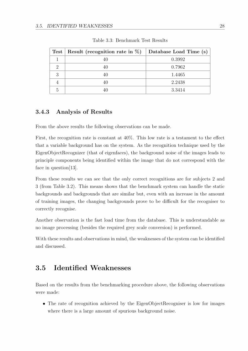
As the bins are stored in an array, the index of the required bin must be calculated. This

is done with the algorithm represented in 4.3 by shifting the value by z (or the zero shift

value which shifts the values, temporarily, into the positive spectrum) as an index of an

array cannot be a negative value. This is mathematically represented by the following

transform which was developed for the purposes of this process:

z = 0− lowerLimit (4.1)

y = d(x + z)/binSizee (4.2)

index =

y − 1 if y 6= 0

0 if y = 0(4.3)

Once the data has been accumulated within the frequency histogram, the outlying data

must be trimmed. This is done by the trim() method of the Histogram object which take

an integer value as a threshold and all bins whose frequency falls below this threshold

value have their frequency set to zero.

Finally, once the trimmed histogram has been obtained, the upper and lower limits of the

histogram can be obtained. This is done by finding all bins who’s frequency is greater than

zero. The lowest of these bins will have its lower limit extracted and used as the lower


limit of the histogram. The highest of the bins will have its maximum value extracted with

that value representing the upper limit of the histogram. These two values are returned

in a two element array.

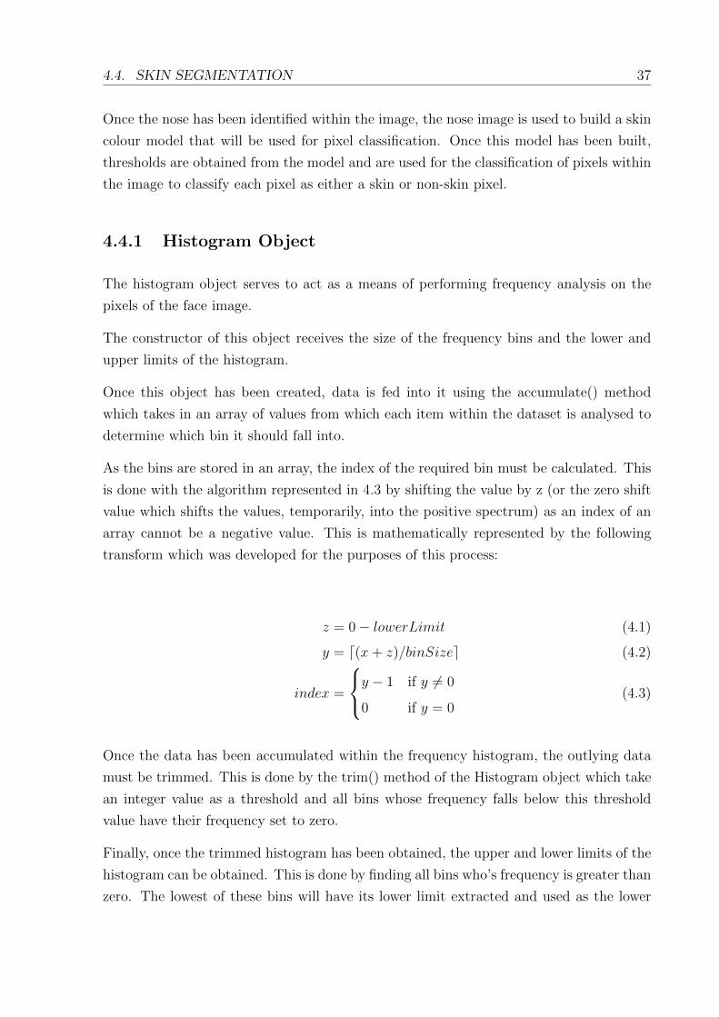
4.4.2 Skin Modeling

Before this model can be built, the colour spaces that are to be used must be decided upon.

This is done within the constructor with a choice between RGB, normalised RGB and

HSV. The constructor receives an integer value as a parameter and uses this to determine

colour space that is to be used for the duration of the segmentation.

Figure 4.7: Colour Space Selection

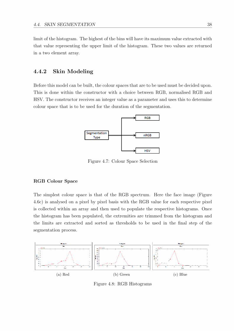
RGB Colour Space

The simplest colour space is that of the RGB spectrum. Here the face image (Figure

4.6c) is analysed on a pixel by pixel basis with the RGB value for each respective pixel

is collected within an array and then used to populate the respective histograms. Once

the histogram has been populated, the extremities are trimmed from the histogram and

the limits are extracted and sorted as thresholds to be used in the final step of the

segmentation process.

(a) Red (b) Green (c) Blue

Figure 4.8: RGB Histograms


Normalised RGB Colour Space

The normalisation of the Red, Green, and Blue values are transformed by the following

transform[14]:

r =R

R + G + B, g =

R

R + G + B, b =

R

R + G + B(4.4)

From the above we can see that the R, G , and B values are transformed into r, g , and

b respectively. The sum of these three new values is equal to one as shown below[14].

r + b + g = 1 (4.5)

Once again, after the transform has been completed, the data is fed to an instance of the

histogram class where the frequency analysis is done once more. Once the histogram has

been accumulated, the outlying values are trimmed and the limits are obtained from it.

These limits then form the thresholds against which the pixels will be classified. During

the classification process, each pixel being scrutinised must also have their RGB values

normalised before the thresholds can be applied.

The use of the normalise RGB colour space has shown to reduce the lighting effects

within the image itself. This can be advantageous as one of the identified weaknesses of

the benchmark system was susceptibility to changes in the lighting conditions [14] .

HSV Colour Space

The HSV colour space describes the colour of a pixel not by its RGB values but by its

Hue, Saturation and Value [10]. The Hue value of the pixel serves to describe dominant

colour of the pixel, the Saturation serves to describe the degree to which that dominant

colour is present, and the Value component is used to store the information regarding

brightness [14].

The HSV colour space requires a non-linear transformation of the RGB values to arrive

at the corresponding HSV values [14]. The transformation is shown in:


v = maxr,g,b (4.6)

s =maxr,g,b −minr,g,b

v(4.7)

h =

g−b

6(maxr,g,b−minr,g,b)if v = r

2−r+b6(maxr,g,b−minr,g,b)

if v = g

4−g+r6(maxr,g,b−minr,g,b)

if v = b

(4.8)

As with the normalised RGB colour space, during the classification process, each pixels

RGB values must undergo the transform before the thresholds can be applied.

4.4.3 Segmentation

Once the thresholds have been computed with the use of the pixel colour frequency his-

tograms, the image is analysed on a pixel by pixel basis once more to apply the afore-

mentioned thresholds. If the pixel falls within the thresholds, it is deemed to be a skin

pixel and is left alone. If it falls out of the thresholds, it is deemed a non-skin pixel and

has the RGB values changed to a predetermined value1.

The result of this process is depicted below in Figure 4.9.

(a) Input Image (b) Segmented Image

Figure 4.9: Segmentation

From the above image, we can see most if not all of the background noise is removed

1For the purposes of representations in this document, that value has been set to (0, 255, 0) or green.Within the actual system, it is set to (255, 255, 255) or white as this has shown to produce better resultsin the testing phase.

4.5. FACE RECOGNISER 41

leaving only skin pixels within the image. While some of the skin pixels have been wrongly

classified, the majority of the pixels have been classified correctly. Also noticeable in this

image is the complication caused by facial hair. This is because, as seen on the chin of

the face in the image, the facial hair is darker than the skin model built from the nose

and thus is deemed to be non-skin pixels. While semantically this is correct (as hair is

technically not skin), those pixels still form part of the face and thus should not, ideally,

have their RGB values changed.

4.5 Face Recogniser

Once the input images have been segmented, they are passed to the constructor of the

EigenRecogniser object. Along with this array of segmented images, an array of strings

is also passed to the array which contains the true names of each respective image. Once

these arrays have been stored within the object, the learn() function is called.

This array of images and strings serves as the training data for the recogniser to be used

in the calculation of the PCA subspace and the projection thereof.

The training of the EigenRecogniser is depicted in Figure 4.10

Figure 4.10: Recogniser Training Algorithm

4.5.1 Principle Component Analysis

As mentioned above, the basis of the face recognition component is the Eigenfaces tech-

nique. This technique makes use of Principle Component Analysis (whose internal working

were expanded on in Chapter 2) to extract the features of the face that are deemed most

important.

The calculation of the eigenvectors and the average image is done by the static member

function of the EigenObjectRecognizer. This method takes an array of grey scale images

and an instance of MCvTermCriteria. The first acts as the set of training images that will


be used to calculate the eigenvectors. The MCvTermCriteria is used as the termination

criteria that is needed of the PCA algorithm to be completed. For the purpose of this

system, as the number of training images is not too great, the termination criteria is

set to the number training images minus 1. Once this has been done, two items are

returned from the function, those being a jagged array of float values that represent the

eigenvectors and a grey scale image that represents the average face generated from the

input face array.

This method serves at creating the PCA subspace against which the training images are

projected to obtain the eigenvalues for each image.

Both of these returned items are used in the next step of the training process, that of

projection.

4.5.2 Projection

Once the eigenvectors have been obtained along with the average image, each of the

training images are projected onto the PCA subspace. From this, the eigenvalues are

obtained and saved to another jagged array to be used later in the recognition process.

This process is done by another static method of the EigenObjectRecognizer class, the

EigenDecomposite(). This method taken in the following parameters[3]:

• The image that is to be projected onto the PCA subspace.

• The eigenimages that were created in the generation of the PCA subspace.

• The average face image that was also generated in the step mentioned above.

4.5.3 Recognition

The main objective of the recogniser object is to compare an input image against those

in the database to determine which it is most similar to. This process is similar to the

training process in the static method EigenDecomposite is once more called from the

EigenObjectRecognizer. The eigenvalues are then obtained from this method and is then

used in the calculation of the nearest neighbour.

Once the eigenvalues have been calculated for the input image, they are compared to the

eigenvalues saved during the training phase. This comparison compares the Euclidean


Distance between the input image and the training images in the PCA subspace. This is

shown below in Figure 4.11.

Figure 4.11: Finding the Nearest Neighbor

Here we can see that a variant of the Euclidean Distance formula is used. While the

formula for the Euclidean Distance is shown below [8], it can be seen that the square root

is not applied to the value. As the square root does not affect the relationship between

the two points, it is removed so as to reduce the amount of required computations:

d(xi, xj) =n∑

r=1

(ar(xi)− ar(xj))2 (4.9)

Finally, once the shortest Euclidean Distance has been identified and the index saved,

the index is returned as the index of the nearest neighbour. However, if the distance to

the nearest neighbour is greater than the threshold value, a value of -1 is return as the

neighbour has been deemed to be too far to be regarded as a reliable recognition.

Once the index has been returned, a check must first be done to verify the validity of the

recognition. This is done by checking the value of the returned index. If it equal to -1,

then an empty string is returned as the label as no recognition has been made. If not,

the index is used to identify the image label from the label array and that indexed value

is returned as the identified individual.


4.6 Chapter Summary

The system developed for the purposes of this research was comprised of three components,

those being the Face Detector, the Skin Segmentation component, and finally the Eigen

Recogniser. These components were designed and developed with the aim of creating a

more robust facial recognition system.

The face recogniser makes use of a Haar classifier that is supplied by the EmguCV package

and is pre-trained. Once the face is detected within the image, the area without the face

in is cropped, thereby greatly reducing the amount of background noise in the training

image.

This cropped image is then passed to the Skin Segmentation component for further noise

reduction. In this component, the nose of the face is detected (using another provided,

pre-trained haar classifier) and is used to build a skin model based on the chosen colour

space. This modelling process results in a set of thresholds that can be used to classify

the pixels in the face image as either skin or non-skin with the non-skin pixels being set

to a predetermined value.

Finally, the cropped and segmented images are passed to the recogniser where the train-

ing process takes place. This process involves the creation of a PCA subspace and the

subsequent projection of each training image onto this subspace. The values obtained for

this are then stored within the newly trained recogniser.

The recognition process therefore involves the projection of the test image onto the PCA

subspace and then the identification of the nearest neighbour. Depending on the distance

to this neighbour, a positive recognition is either returned or not.

In the following chapter, the testing of this system is explored with results and analysis

thereof.

Chapter 5

Experimental Design and Results

5.1 Introduction

This chapter will explore the performance of this developed system against the perfor-

mance of the benchmark system described in Chapter 3. Both of these systems will be

tested using the same testing framework and image database described in Chapter3. Once

the performances of the two systems have been juxtaposed, analysis is done in an attempt

to understand the difference in performance.

The purpose of this juxtaposition is to determine whether the components described and

implemented in Chapter 4 have created a more robust facial recognition system that can

fulfill most, if not all, of the requirements described in Chapter 1.

5.2 Design

For the purposes of testing the performance of the developed system, it will be tested

by two frameworks. The first of which is the framework identified in Chapter 3. As

the benchmark system underwent the same tests, it will provide a point of comparison

between the benchmark system and the developed system.

Then, for more detailed analysis, the developed system will undergo the following testing

framework:

45

5.3. RESULTS 46

Table 5.1: Framework 2 Description

Test 1 5 test images and one training image per individual

Test 2 4 test images and 2 training images per individual



Test 5 one test image and 5 training images per individual

The Euclidean Distance to matches will also be measured along with the time taken to

load the images into the database.

Finally, the applied threshold of the system will be tested on its ability to reject faces not

within the system.

5.3 Results

A basic test of one test image and varying amounts of training images is listed below

(from Table 3.1 against which the benchmark system was also tested).

Table 5.2: Robust System Basic Test Results

Test Result (recognition rate in %) Database Load Time (s)

1 60 22.0008

2 60 28.4859

3 60 31.4892

4 80 38.2192

5 80 45.2049

A more detailed set of tests produced the following set of results1. When the system was

run through the same testing framework as mentioned above, the following results were

obtained.

1The use of the HSV colour space produce no better results than the use of the RGB colour space andthus, the results shown are from the use of the RGB colour space only.

5.3. RESULTS 47

Table 5.3: Framework 2 Test Results

Test Result (recognition rate in %)

1 32%

2 30%

3 46.67%

4 70%

5 80%

This data is then transformed from a test by test analysis to a subject by subject analysis.

Table 5.4: Subject Analysis

Subject Test 1 Result Test 2 Result Test 3 Result Test 4 Result Test 5 Result

1 0% 50% 33.3% 100% 100%

2 20% 25% 0% 100% 100%

3 0% 0% 66.6% 100% 100%

4 60% 75% 66.6% 50% 100%

5 80% 0% 66.6% 0% 0%

When testing the application of a threshold for the purposes of rejecting a subject that

is not in the database of the system, the following results were obtained:

Figure 5.1: Threshold Testing

5.4. ANALYSIS OF RESULTS 48

Within the graph listed in Figure 5.1, it should be noted that Face 4 represents a positive

recognition, Face 5 represents a negative recognition, and Object refers to an inanimate

object and therefore an image that is not within the image database of the system.

All tests were run with both histogram equalisation present and again without it. As both

sets of tests yielded the same results, the use of histogram equalisation has been deemed

ineffective for use in this system.

5.4 Analysis of Results

The HSV colour space showing no improvement in recognition rate is shown to be a

result of the size of the image database, as it has been shown to be of better use in a

facial recognition system than the RGB colour space [10].

From the table above (Table 5.2), it can be seen that in the majority of the test cases within

the basic tests, the developed system performs at levels that are double the performance of

the benchmark system. As one of the main purposes of the system is to reduce the amount

of spurious background noise within the image before it is passed to the recogniser, it can

be assumed that it is this reduction of background noise that leads to a more focus image

and thus a more robust system.

When considering the results obtained from applying the testing framework to the devel-

oped system, it can be seen that there is a progressive increase in the recognition rate

of the system as the framework progresses. When the system only had one training im-

age, the PCA algorithm could not generate a suitable subspace that allowed for a high

recognition rate, thus, the relationship between the number of training images and the

recognition rate appears to be a direct one. While this may be true for the current set

of data, more testing is needed to see if this relationship will eventually plateau, however

this investigation falls out of the scope of this research.

When regarding the subject by subject test data represented in Table 5.4, it can be seen

that in most cases, the relationship mentioned above is maintained. Subjects 1 through

4 both show an increase in recognition rate when the number of training images has

increased. The fringe case of subject 5 is explained as such. According to Table 3.2, the

images recorded for subject 5 involved the capturing of 5 images with a static background

and one image of the face from a varied angle. The recognition rate of Subject 5 is 80%

(Test 1 of Framework 1) due to the fact that the tested images had been taken at short


intervals where the face did not have sufficient time to alter its expression too dramatically.

Thus, these images are extremely similar to the singular training image and thus each is

identified correctly.

A more focused image also leads to a closer match to the specific image in the PCA

subspace. This is represented in the graph below where the Euclidean Distance of the

recognitions is plotted for both the benchmark system and the developed system.

Figure 5.2: Euclidean Distance Comparison

The graph above represents the Euclidean Distance to the nearest neighbour. The sets of

recognition tests were applied to both the benchmark system and the developed system.

From Figure 5.2 we can see the dramatic decrease in the length of the Euclidean Distance

between the matches. As the scale of the graph is logarithmic, even a small improvement

is dramatic. Is some cases, there has been a 99.98% reduction in this distance.

Another point of interest that can be drawn from Figure 5.2 is from the last dataset.

This subject was correctly recognised by neither the benchmark system nor the developed

system. What can be seen from Figure 5.2 is that in a negative recognition, the Euclidean

Distance to the nearest neighbour remains somewhat consistent with the one produced

by the benchmark system, showing that the developed system improves the matches of

positive recognitions and not that of negative recognition.This shows that the developed

system does not simply reduce the Euclidean Distance of every recognition.

Other evidence to support the idea that the image is more focused is that of the average


image produced within the EigenRecogniser. Figure 5.3a represents the average image

generated by the benchmark system. It has various elements of the background included,

some static and constant while others are blurred. Based on the results of the testing,

it can be said that it is this background noise that is causing a lower recognition rate.

Figure 5.3b represents the average image generated by the developed system. Within this

image, the amount of background noise is drastically decreased and the average face of

the individuals is easily discernible.

(a) Benchmark System (b) Developed System

Figure 5.3: Average Image Comparison

While these results have proved to be positive and led to an increase in the recognition

rate, other results have not been as promising.

Firstly, the use of histogram equalisation has proven to have little to no noticeable effect

on the performance of the system. As one of the aims of the developed system to to

reduce the affects of light variability, the results point to the fact that this aim has not

been reached. As mentioned in Chapter 2, the eigenfaces technique is highly susceptible to

varying lighting conditions and as this is implicit in the recognition process, it is inherent

within the system.

The developed system has also proved to be slower than the benchmark system. This is

due to the image processing that each image undergoes during the training and recog-

nition. As can be seen by the graph, this increase in speed is linear. As the number of

training images increases, the time taken to load the image database, from file into the

system, increases. This linear relationship is due to the fact that each image undergoes

the exact same procedure during the image processing. As each image is the same size,


each image has the same number of pixels and thus the time taken to analyse each image

is similar.

Figure 5.4: Timing Comparison

While this presents a scalability problem for the developed systems certain implementation

changes can be made to reduce the effects of this timing difference. These changes are

outlined in the Possible Future Extensions section in Chapter 6.

Finally, the proposed solution of using a threshold as a means of rejecting images that

are not within the database has proven ineffective. This is represented by Figure 5.1.

Here, the Euclidean Distance to the nearest neighbour is depicted. From this, it can be

seen that the distance for the positive recognition is much greater than both the negative

recognition and the inanimate object. Thus, the application of a threshold would prove

ineffective as the positive recognition would be discarded. A possible reason for this is the

size of the image database. If this were to increase (i.e. the number of training images

per subject) a closer match could be obtained and thus the thresholding could become

viable. However, within the current system, it is not a viable means for image rejection.

Thus from these findings and comparisons, it can be seen that a reduction in background

noise leads to less points of interest to be detected during the principle component analysis.

This then leads to a closer match to the desired image and, ultimately towards a higher

recognition rate.


5.5 Chapter Summary

The aim of this chapter was to evaluate the performance of the of the developed system

and to compare it to the performance of the benchmark system outlined in Chapter 3.

When comparing the basic tests performed on both the benchmark system and the de-

veloped system, the following observations were made:

• The developed system consistently produced higher rates of recognition than the

benchmark system.

• In test 5, where the number of training images was at a maximum, the recognition

rate of the developed system was double the rate of the benchmark system.

With more detailed testing of the developed system, the following trends were revealed:

• As the number of training images increased, the recognition rate of the system

increased.

• The system was able to correctly identify all of the subjects except for subject 5

proving that the varied angle of the face is problematic.

• For positive matches, the developed system produces a much closer match than that

of the benchmark system based on the Euclidean Distance to the nearest neighbour.

• The applied threshold (whose aim was to give the system the ability to reject an

image that is not within the system) produced mixed results in that it could reject

some images but not all.

• The use of the histogram equalisation of the lighting conditions within the input

images lead to no noticeable change in the performance of the system and thus, the

system was still susceptible to changes in lighting conditions

• The image processing leads to a dramatic increase in the time taken to load the

database and this linear relationship (between the number of images in the database

and the time taken to load them in the system) leads to a scalability problem within

the system.

The size of the image database has proven to limit the results obtained by the tests and

a larger database could yield better results.

Chapter 6

Conclusion

Based on the analysis of the results obtained in Chapter 5, the following conclusions have

been drawn with the aims of the research as well as the proposed solutions mentioned in

Chapter 3 in mind.

The aim of reducing the background noise of the input image was met. When comparing

the original input image and the final segmented image, it can be seen that there is little

to no background noise left within the image and that it contains mostly the face data

of the individual concerned. This can be seen by the examples presented in Chapter 4,

more specifically the resulting images presented in Figure 4.4c and Figure 4.9b. As has

been shown by the performance of the developed system, this reduction in background

noise has produced an increase in the recognition rate of the system. This is due to the

noise reduction within the image by the facial detection and skin segmentation process.

As shown in Figure 5.3b, the average face produced by the developed system is testament

to this fact.

The aim of reducing the system susceptibility to lighting changes was not reached. The

tools provided by the EmguCV package (such as histogram equalisation) proved to have

no noticeable effect on the performance of the system. The use of the normalised RGB

and HSV colour spaces also proved ineffective. A possible explanation for this is the use

of the eigenfaces technique for recognition. As mentioned in Chapter 2, this technique is

implicitly susceptible to changes in lighting conditions. Another possible reason for this

is the size of the image database. As mentioned in Chapter 5, the size of the database

seems to limit the results of the system.

The adding of the threshold to the nearest neighbour matching within the recognition

53

6.1. POSSIBLE FUTURE WORK 54

algorithm provided mixed results. Images that contained irrelevant objects such as chairs

and other inanimate objects produced a Euclidean Distance that was not able to be dif-

ferentiated from a positive match. While other faces tested that were not in the database

proved to produce varying distances. This makes the use of the thresholds inconsistent

and while they have been shown to work at some times, there have been times when they

have been proven ineffective.

Finally, while the system has been shown to be more robust in the nature of the images

that it can recognise, the process of background noise removal (namely the face detection

and skin segmentation) has led to potential scalability problems. As shown in Figure 5.4,

the load time of the image database using the developed system is substantially greater

than that of the benchmark system. With a linear relationship, adding more images to

the database will lead to a constant increase in the database load time with the current

implementation.

Ultimately, while the system as shown to have some drawbacks, it has produced better

recognition results than the generic recogniser provided in the EmguCV package with

images that had varying backgrounds with various amount of background noise. Thus,

it can be said that the system is robust even though it does not fulfill all of the aims set

out in Chapter 1.

With the above conclusions regarding the research and results thereof in mind, the fol-

lowing future extensions have been proposed.

6.1 Possible Future Work

As the field of facial recognition is vast and constantly expanding, there is constant space

for improvement. With regards to the developed system, the following aspects have been

proposed as future extensions to the system.

The current data set used for the testing of this system is relatively small when compared

to the standard databases provided online. To extend this research and perhaps improve

the results of the system, the database could be expanded. It has already been shown

that an increase in the number of training images leads to an increase in the recognition

rate of this system, therefore an expanded image database should be able to improve the

performance of the system.

Another possibility for future works is the comparison of face recognition techniques. As


mentioned in Chapter 4, this research only makes use of the eigenfaces technique. Other

techniques, such as artificial neural networks and hybrid systems, can be tested and the

results compared to identify which of the techniques is more suited to the aims of this

research.

As mentioned in the previous chapter, the developed systems loading of the database is

almost fifteen times longer than that of the benchmark system. This is due to the image

processing done on each image within the database. A possible method of improving this

load time is parallelism. By parallelising the pre-processing of the database, many of the

database images can be processed simultaneously. As each of the images undergoes the

same procedure and there are no resources that need to be shared by these procedures,

the method of parallelism is well suited to this task.

Another extension that can be implemented is to the skin segmentation component. There

are other colour spaces that have proved to be effective in the field of skin segmentation

such as TSL. These have shown to produce a more exact skin model and have the potential

to produce a better segmented image [10].

Also in the field of skin segmentation, the actual segmentation process can be altered to

create an image with even more noise reduction. This can be done by cropping the image

both vertically and horizontally such that the image is made smaller till the border of the

image is touching the border of the face without reducing the total number of skin pixels

within the face. This process is demonstrated in Figure6.1.

Figure 6.1: Movement of the Bounding Box

Finally, the current system can be fooled by holding up a photograph of an individual.

The system will view this as a real individual and perform the recognition on it. There

are various methods for the prevention of such an act such as a two stage image capture

process in which the lighting conditions of the environment are changed in an attempt to

create shadows around the nose and eye area. If these shadows are not present within the

second image, the image can be regarded as a two dimensional individual and discarded


while if the shadows are present, the individual can be classified as three dimensional and

the process can continue.

Bibliography

[1] Face Detection and Identification. Online, July 2008. Available from:

http://www.emgu.com/forum/viewtopic.php?f=7t=11.

[2] Face Detection. Online, June 2010. Available from:

http://www.emgu.com/wiki/index.php/Face detection.

[3] EigenObjectRecognizer Class. Online, 2011. Available from:

http://www.emgu.com/wiki/files/2.3.0/document/Index.html.

[4] Bouzerdoum, S. L.-P. A., and Chai, D. Skin segmentation using color and

edge information. In Proc. Int. Symposium on Signal Processing and its Applications

(2003).

[5] Bradski, G., and Kaehler, A. Learning OpenCV: Computer Vision with the

OpenCV Library. O’REILLY, 2008.

[6] Hjelmas, E., and Low, B. K. Face detection: A survey. Computer Vision and

Image Understanding 83 (2001), 236–274.

[7] Lemieux, A., and Parizeau, M. Experiments on eigenfaces robustness. In Pro-

ceedings of the 16 th International Conference on Pattern Recognition (ICPR’02)

Volume 1 - Volume 1 (Washington, DC, USA, 2002), ICPR ’02, IEEE Computer

Society, pp. 10421–.

[8] Lin, S.-H. An introduction to face recognition technology. Informing Science Special

Issue on Multimedia informing Technologies - Part 2 3 (2000), 1–7.

[9] Miano, J. Compressed image file formats: JPEG, PNG, GIF, XBM, BMP. Addison

Wesley Longman, Inc., 2000.

57

BIBLIOGRAPHY 58

[10] Phung, S.L.; Bouzerdoum, A. S. C. D. S. Skin segmentation using color pixel

classification: analysis and comparison. Pattern Analysis and Machine Intelligence

27 (2005), 148 – 154.

[11] P.Latha, Dr.L.Ganesan, D. Face recognition using neural networks. Signal

Processing: An International Journal 3 (2009), 153–160.

[12] Reda, A.; Aoued, B. Artificial neural network-based face recognition. In Con-

trol, Communications and Signal Processing, 2004. First International Symposium

on (2004).

[13] Turk, M., and Pentland, A. Eigenfaces for recognition. Journal of Cognitive

Neuroscience 3 (1991), 71– 86.

[14] V. Vezhnevets, V. S., and Andreev, A. A survey on pixel-based skin color

detection techniques. Proceedings of the Graphicon 85 (2003), 85–92.

[15] Viola, P., and Jones, M. Rapid object detection using a boosted cascade of

simple features. pp. 511–518.

Appendix A

Glossary

ANN Artificial Neural Network

DNA Deoxyribonucleic Acid

KL Karhonen-Loeve

FPS Frames Per Second

FRS Facial Recognition System

PCA Principle Component Analysis

RAM Random Access Memory

HSV Hue, Saturation, Value

RGB Red, Green, Blue

ROI Region of Interest

TSL Tint, Saturation, Lightness

YCbCr Luminance and Chrominance

59

building a robust facial recognition system based … · building a robust facial recognition...

Documents