budgeting given expected sales forecasts, sales price, and cash collections policies, be able to...
TRANSCRIPT

Budgeting
ENGM 661Engineering Economics
for Managers
Given expected sales forecasts, sales price, and cash collections policies, be able to prepare a sales budeget.
Given expected sales and inventory policies, be able to prepare a production, materials, and direct labor cost budgets.
Given a budget and actual cost figures, be able to compute and interpret budget to cost variances.
Learning Objectives

Set ObjectivesBottom Up vs Top DownSales ForecastHistorical DataNon-Financial ParametersResponsibility Accounting
Budget Guidelines

ProfitIncreased market shareReturn on InvestmentCost ReductionRevenue increases
Setting Objectives

Iterative ProcessYou cannot ask a manager at any level to
accept responsibility for living within budgets that he or she had no hand in setting.
Bottom Up vs Top Down
Operating BudgetSales Production Direct Materials/Labor Factory OverheadPro-forma income
Financial BudgetCash Pro-forma balance sheet
Categories
Prepare sales forecastDetermine aggregate productionEstimate manufacturing costs & operating
exp.Determine cash flowFormulate project financial statements
Preparation

Sales Budget
Production Budget
Direct Material
Factory Overhead
Direct Labor
Cost of GoodSold Budget
Selling Expense
Admin Expense
Budgeted Income
Budgeted Balance
Desired Ending
Inventory
Capital Budget Cash Budget
Sales ForecastK-Corp Income Statement
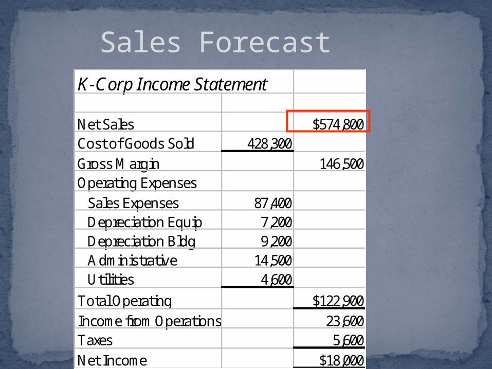
Net Sales $574,800Cost of Goods Sold 428,300Gross Margin 146,500Operating Expenses Sales Expenses 87,400 Depreciation Equip 7,200 Depreciation Bldg 9,200 Administrative 14,500 Utilities 4,600
Total Operating $122,900Income from Operations 23,600Taxes 5,600Net Income $18,000
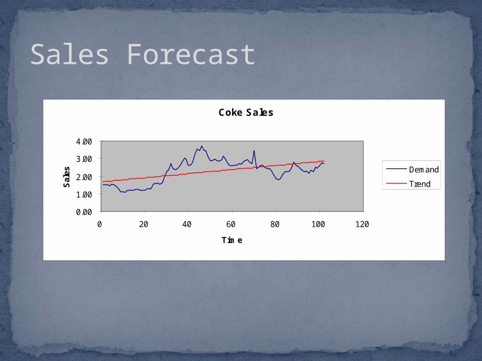
Sales Forecast
Coke Sales
0.00
1.00
2.00
3.00
4.00
0 20 40 60 80 100 120
Time
Sal
es Demand
Trend

Sales Forecast
Coke Sales
0.00
1.00
2.00
3.00
4.00
0 20 40 60 80 100 120
Time
Sal
es Demand
Trend
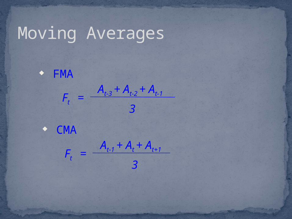
Moving Averages
CMA
FMA
Ft =3
At-3 + At-2 + At-1
Ft =3
At-1 + At + At+1
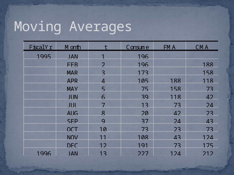
Moving AveragesFiscal Yr Month t Consume FMA CMA
1995 JAN 1 196FEB 2 196 188MAR 3 173 158APR 4 105 188 118MAY 5 75 158 73JUN 6 39 118 42JUL 7 13 73 24AUG 8 20 42 23SEP 9 37 24 43OCT 10 73 23 73NOV 11 108 43 124DEC 12 191 73 175
1996 JAN 13 227 124 212
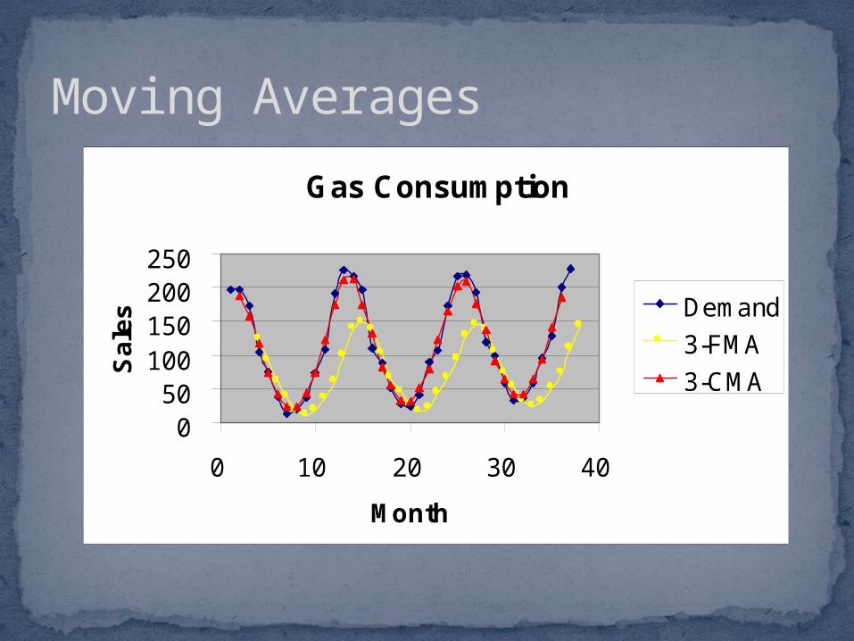
Moving Averages
Gas Consumption
050
100150200250
0 10 20 30 40
Month
Sa
les Demand
3-FMA
3-CMA
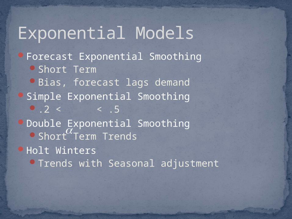
Forecast Exponential SmoothingShort TermBias, forecast lags demand
Simple Exponential Smoothing.2 < < .5
Double Exponential SmoothingShort Term Trends
Holt WintersTrends with Seasonal adjustment
Exponential Models
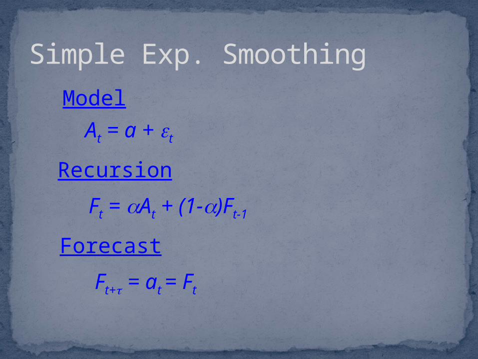
Simple Exp. Smoothing
Model
At = a + t
Recursion
Ft = At + (1-)Ft-1
Forecast
Ft+= at = Ft
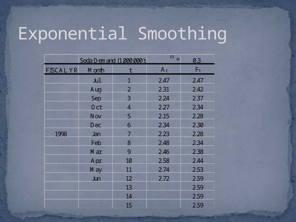
Exponential SmoothingSoda Demand (1,000,000's) a = 0.3
FISCAL YR Month t At Ft
Jul 1 2.47 2.47Aug 2 2.31 2.42Sep 3 2.24 2.37Oct 4 2.27 2.34Nov 5 2.15 2.28Dec 6 2.34 2.30
1998 Jan 7 2.23 2.28Feb 8 2.48 2.34Mar 9 2.46 2.38Apr 10 2.58 2.44May 11 2.74 2.53Jun 12 2.72 2.59
13 2.5914 2.5915 2.59

Exponential Smoothing
Soda Consumption
1.5
2.0
2.5
3.0
0 5 10 15
Month
Sal
es Demand
ExpSmth
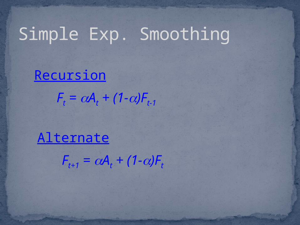
Simple Exp. Smoothing
Recursion
Ft = At + (1-)Ft-1
Alternate
Ft+1 = At + (1-)Ft
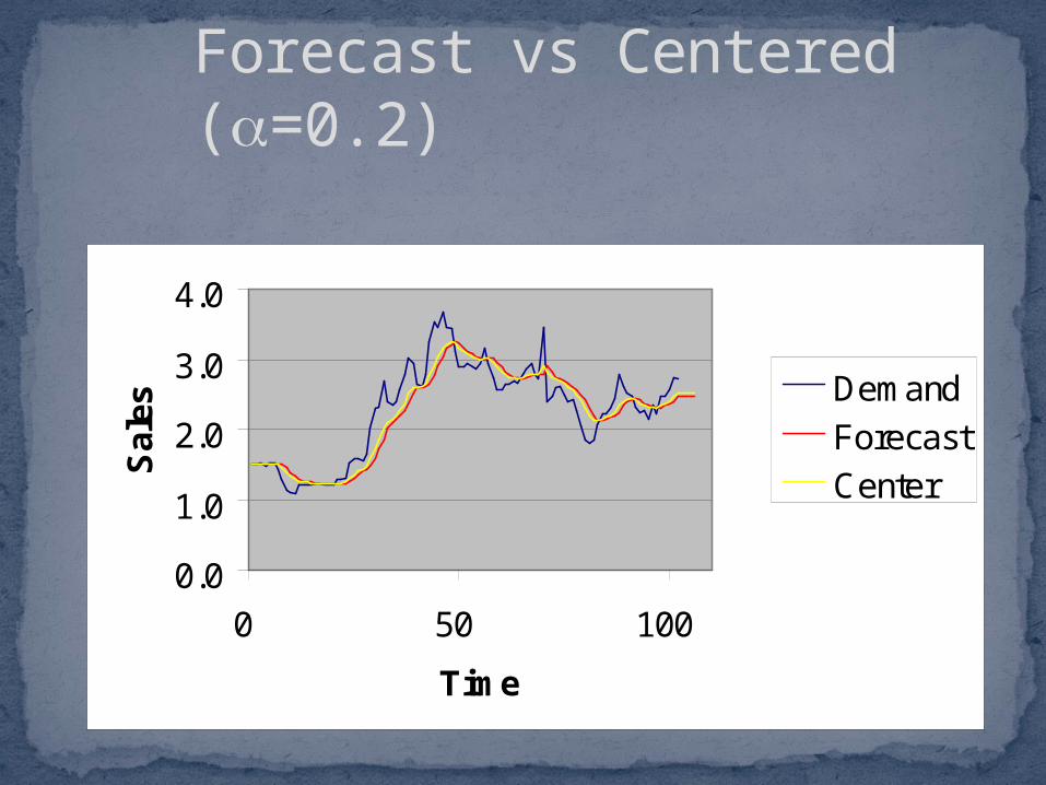
Forecast vs Centered (a=0.2)
0.0
1.0
2.0
3.0
4.0
0 50 100
Time
Sal
es
Demand
Forecast
Center

0.0
1.0
2.0
3.0
4.0
0 50 100
Time
Sa
les Demand
Forecast
Forecast vs Centered (a=1.0)
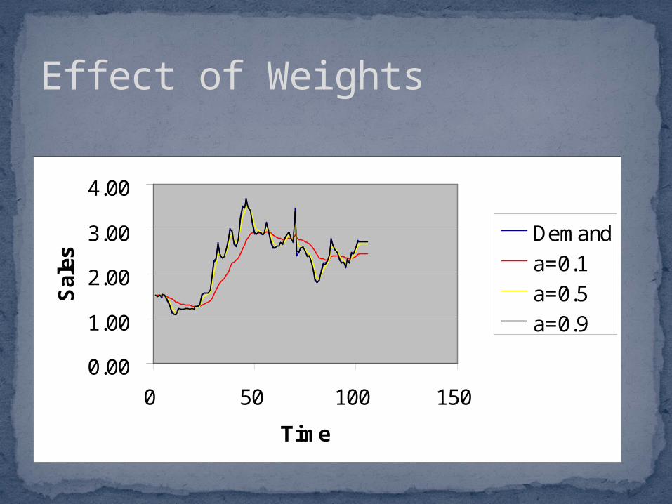
Effect of Weights
0.00
1.00
2.00
3.00
4.00
0 50 100 150
Time
Sal
es
Demand
a=0.1
a=0.5
a=0.9

Effect of Weights
a
a
= = +==
= = +=
-
-
-
0 0 0 0 10
10 10 0 0
1
1
1
1
. . .
. . .
F A F
F
F
F A F
A
t t t
t
t t t
t
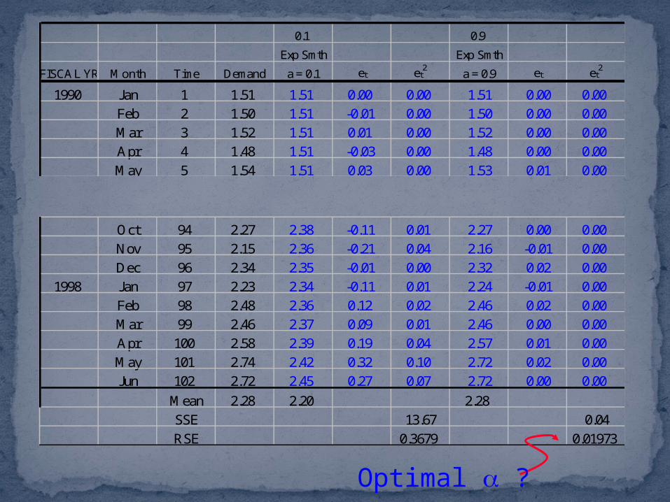
Oct 94 2.27 2.38 -0.11 0.01 2.27 0.00 0.00Nov 95 2.15 2.36 -0.21 0.04 2.16 -0.01 0.00Dec 96 2.34 2.35 -0.01 0.00 2.32 0.02 0.00
1998 Jan 97 2.23 2.34 -0.11 0.01 2.24 -0.01 0.00Feb 98 2.48 2.36 0.12 0.02 2.46 0.02 0.00Mar 99 2.46 2.37 0.09 0.01 2.46 0.00 0.00Apr 100 2.58 2.39 0.19 0.04 2.57 0.01 0.00May 101 2.74 2.42 0.32 0.10 2.72 0.02 0.00Jun 102 2.72 2.45 0.27 0.07 2.72 0.00 0.00
Mean 2.28 2.20 2.28SSE 13.67 0.04RSE 0.3679 0.01973
0.1 0.9
Exp Smth Exp Smth
FISCAL YR Month Time Demand a = 0.1 et et2
a = 0.9 et et2
1990 Jan 1 1.51 1.51 0.00 0.00 1.51 0.00 0.00Feb 2 1.50 1.51 -0.01 0.00 1.50 0.00 0.00Mar 3 1.52 1.51 0.01 0.00 1.52 0.00 0.00Apr 4 1.48 1.51 -0.03 0.00 1.48 0.00 0.00May 5 1.54 1.51 0.03 0.00 1.53 0.01 0.00
Optimal a ?
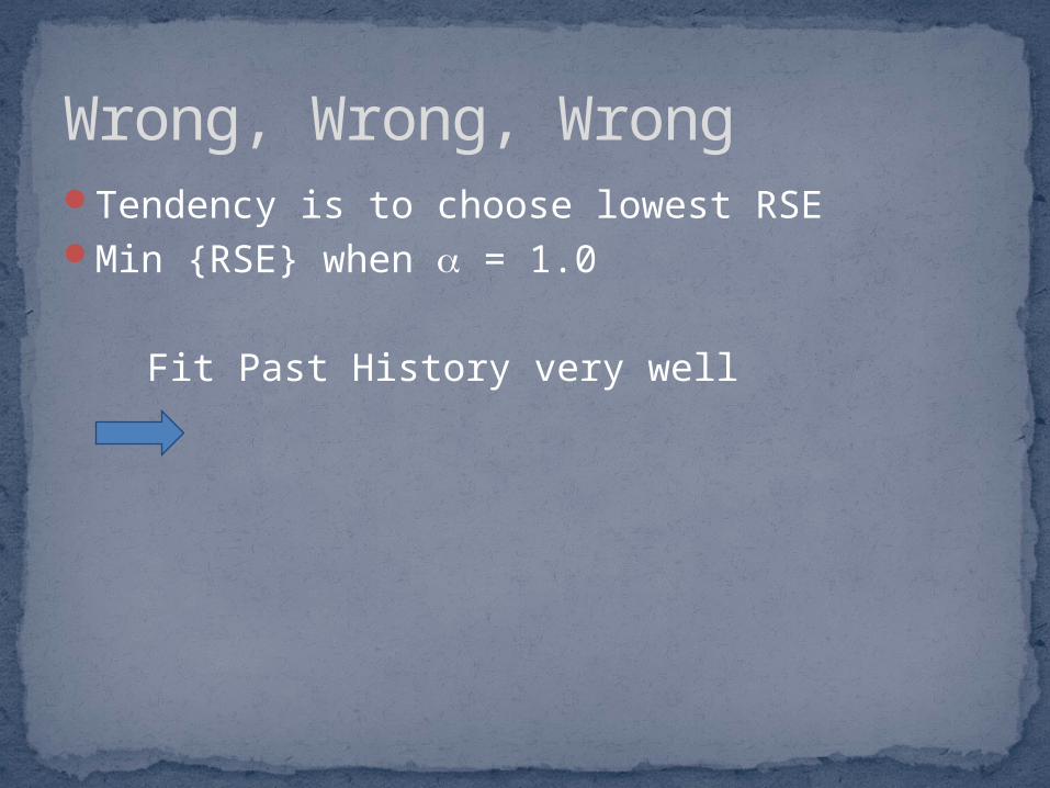
Tendency is to choose lowest RSEMin {RSE} when a = 1.0
Fit Past History very well
Wrong, Wrong, Wrong

Tendency is to choose lowest RSEMin {RSE} when a = 1.0
Fit Past History very well
Divide data into two sets {t=1:60}, {t=61:101}
Wrong, Wrong, Wrong

Past Fit vs Prediction
0.0
1.0
2.0
3.0
4.0
0 50 100
Time
Sa
les Demand
a = 0.1
a = 0.9

0.1 0.9
Exp Smth Exp Smth
FISCAL YR Month Time Demand a = 0.1 et et2
a = 0.9 et et2
1990 Jan 1 1.51 1.51 0.00 0.00 1.51 0.00 0.00Feb 2 1.50 1.51 -0.01 0.00 1.50 0.00 0.00Mar 3 1.52 1.51 0.01 0.00 1.52 0.00 0.00Apr 4 1.48 1.51 -0.03 0.00 1.48 0.00 0.00May 5 1.54 1.51 0.03 0.00 1.53 0.01 0.00
Oct 94 2.27 2.49 -0.22 0.05 1.88 0.39 0.15Nov 95 2.15 2.49 -0.34 0.12 1.88 0.27 0.07Dec 96 2.34 2.49 -0.15 0.02 1.88 0.46 0.21
1998 Jan 97 2.23 2.49 -0.26 0.07 1.88 0.35 0.12Feb 98 2.48 2.49 -0.01 0.00 1.88 0.60 0.36Mar 99 2.46 2.49 -0.03 0.00 1.88 0.58 0.34Apr 100 2.58 2.49 0.09 0.01 1.88 0.70 0.49May 101 2.74 2.49 0.25 0.06 1.88 0.86 0.74Jun 102 2.72 2.49 0.23 0.05 1.88 0.84 0.70
Mean 2.28 2.22 2.18SSE 14.18 6.47RSE 0.37467 0.25301

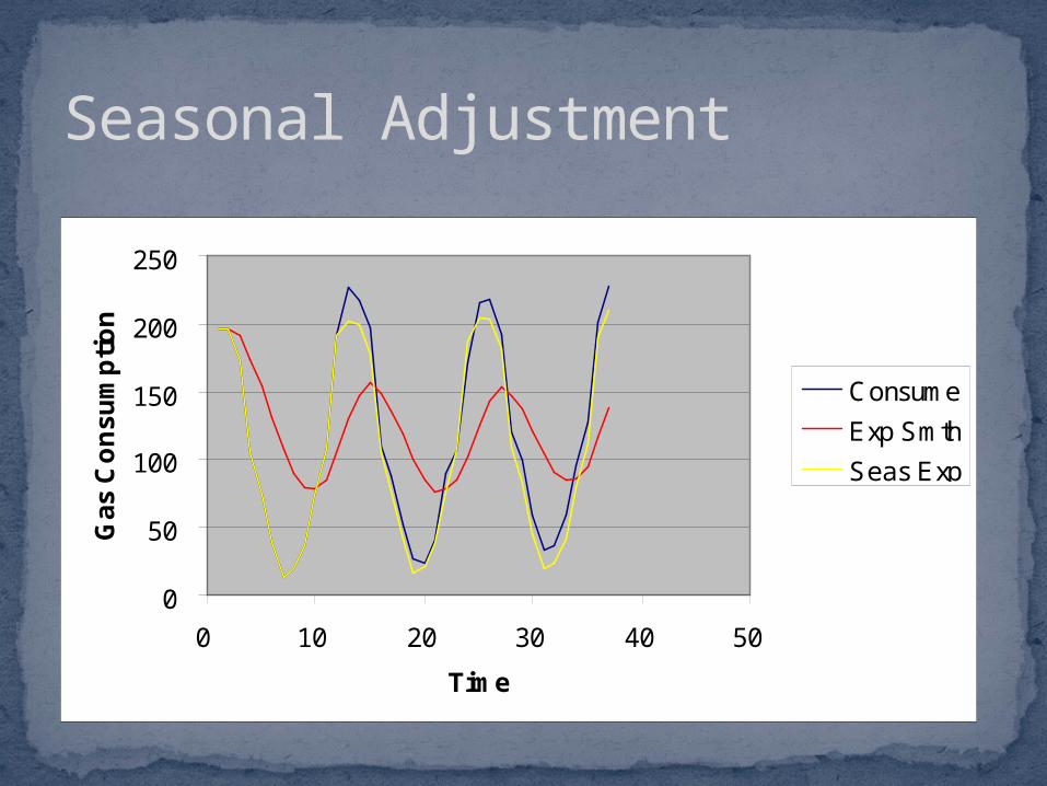
Seasonal Adjustment
0
50
100
150
200
250
0 10 20 30 40 50
Time
Ga
s C
on
su
mp
tio
n
Consume
Exp Smth

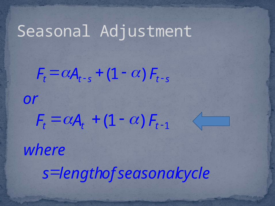
Seasonal Adjustment
F A Ft t s t s= + -
where
s lengthof seasonalcycle=
- -a a( )1
F A Ft t t= + - -a a( )1 1
or
Seasonal Adjustment
F A Ft t s t s= + -
where
s lengthof seasonalcycle=
- -a a( )1
F A Ft t t= + - -a a( )1 1
or
Seasonal Adjustment
0
50
100
150
200
250
0 10 20 30 40 50
Time
Ga
s C
on
su
mp
tio
n
Consume
Exp Smth
Seas Exp

Double Exp. Smoothing
Model
At = a + bt + t
Forecast
Ft+ = at + bt
Recursion
1.
4.
Ft = At + (1-)Ft-1
2. Ft = Ft + (1-)Ft-1
^ ^
3. at = 2Ft - Ft
^
bt = (Ft - Ft)^
1-
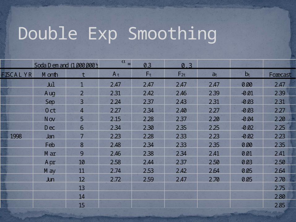
Double Exp Smoothing
Soda Demand (1,000,000's) a = 0.3 0.3
FISCAL YR Month t At Ft F2t at bt Forecast
Jul 1 2.47 2.47 2.47 2.47 0.00 2.47Aug 2 2.31 2.42 2.46 2.39 -0.01 2.39Sep 3 2.24 2.37 2.43 2.31 -0.03 2.31Oct 4 2.27 2.34 2.40 2.27 -0.03 2.27Nov 5 2.15 2.28 2.37 2.20 -0.04 2.20Dec 6 2.34 2.30 2.35 2.25 -0.02 2.25
1998 Jan 7 2.23 2.28 2.33 2.23 -0.02 2.23Feb 8 2.48 2.34 2.33 2.35 0.00 2.35Mar 9 2.46 2.38 2.34 2.41 0.01 2.41Apr 10 2.58 2.44 2.37 2.50 0.03 2.50May 11 2.74 2.53 2.42 2.64 0.05 2.64Jun 12 2.72 2.59 2.47 2.70 0.05 2.70
13 2.7514 2.8015 2.85

Double Exp Smoothing
Soda Consumption
1.5
2.0
2.5
3.0
0 5 10 15 20
Month
Sal
es
Demand
Exp Smooth
Dbl Smooth
Forecast

Holt-Winters Model
where St = Seasonal Factor for time period t
Recursion1. Compute Seasonal factors St 2. Deseasonalize data3. Double smooth on deasonalized data
Forecast
Ft+= (at + bt)St+
Model
At = (a + bt)St te+

Holt-Winters
Soda Consumption
0.01.02.03.04.0
0 40 80 120
Month
Sal
es Demand
Forecast

Sales Forecast
Coke Sales
0.00
1.00
2.00
3.00
4.00
0 20 40 60 80 100 120
Time
Sal
es Demand
Trend
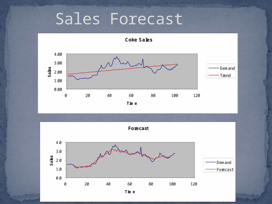
Sales Forecast
Forecast
0.0
1.0
2.0
3.0
4.0
0 20 40 60 80 100 120
Time
Sal
es
Demand
Forecast
Coke Sales
0.00
1.00
2.00
3.00
4.00
0 20 40 60 80 100 120
Tim e
Sal
es Demand
Trend
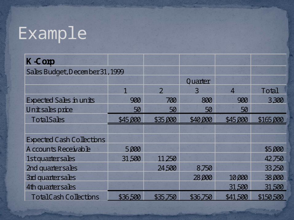
ExampleK-CorpSales Budget, December 31, 1999
Quarter1 2 3 4 Total
Expected Sales in units 900 700 800 900 3,300Unit sales price 50 50 50 50 Total Sales $45,000 $35,000 $40,000 $45,000 $165,000
Expected Cash CollectionsAccounts Receivable 5,000 $5,0001st quarter sales 31,500 11,250 42,7502nd quarter sales 24,500 8,750 33,2503rd quarter sales 28,000 10,000 38,0004th quarter sales 31,500 31,500 Total Cash Collections $36,500 $35,750 $36,750 $41,500 $150,500
Example (cont.)
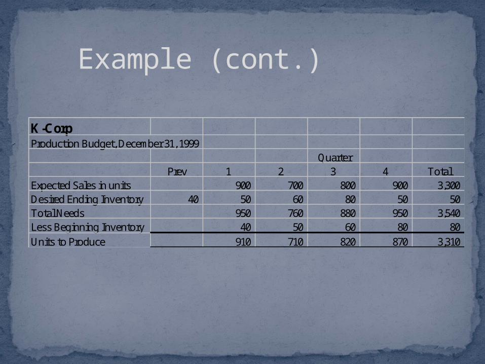
K-CorpProduction Budget, December 31, 1999
QuarterPrev 1 2 3 4 Total
Expected Sales in units 900 700 800 900 3,300Desired Ending Inventory 40 50 60 80 50 50Total Needs 950 760 880 950 3,540Less Beginning Inventory 40 50 60 80 80Units to Produce 910 710 820 870 3,310
Example (cont.)
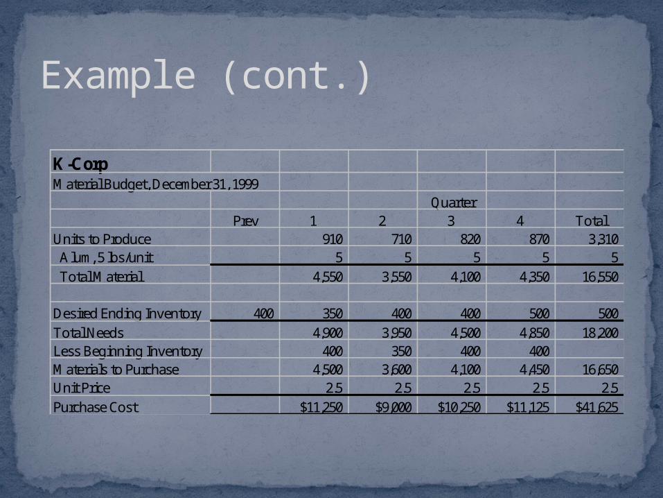
K-CorpMaterial Budget, December 31, 1999
QuarterPrev 1 2 3 4 Total
Units to Produce 910 710 820 870 3,310 Alum, 5 lbs/unit 5 5 5 5 5 Total Material 4,550 3,550 4,100 4,350 16,550
Desired Ending Inventory 400 350 400 400 500 500Total Needs 4,900 3,950 4,500 4,850 18,200Less Beginning Inventory 400 350 400 400Materials to Purchase 4,500 3,600 4,100 4,450 16,650Unit Price 2.5 2.5 2.5 2.5 2.5Purchase Cost $11,250 $9,000 $10,250 $11,125 $41,625

Example (cont.)
K-CorpMaterial Budget, December 31, 1999
QuarterPrev 1 2 3 4 Total
Units to Produce 910 710 820 870 3,310 Alum, 5 lbs/unit 5 5 5 5 5 Total Material 4,550 3,550 4,100 4,350 16,550
Desired Ending Inventory 400 350 400 400 500 500Total Needs 4,900 3,950 4,500 4,850 18,200Less Beginning Inventory 400 350 400 400Materials to Purchase 4,500 3,600 4,100 4,450 16,650Unit Price 2.5 2.5 2.5 2.5 2.5Purchase Cost $11,250 $9,000 $10,250 $11,125 $41,625
Cash DisbursementsAccounts Payable 3,500 3,5001st quarter purchases 5,625 5,625 11,2502nd quarter purchases 4,500 4,500 9,0003rd quarter purchases 5,125 5,125 10,2504th quarter purchases 5,563 5,563 Total Cash Outlay $9,125 $10,125 $9,625 $10,688 $39,563
Example (cont.)
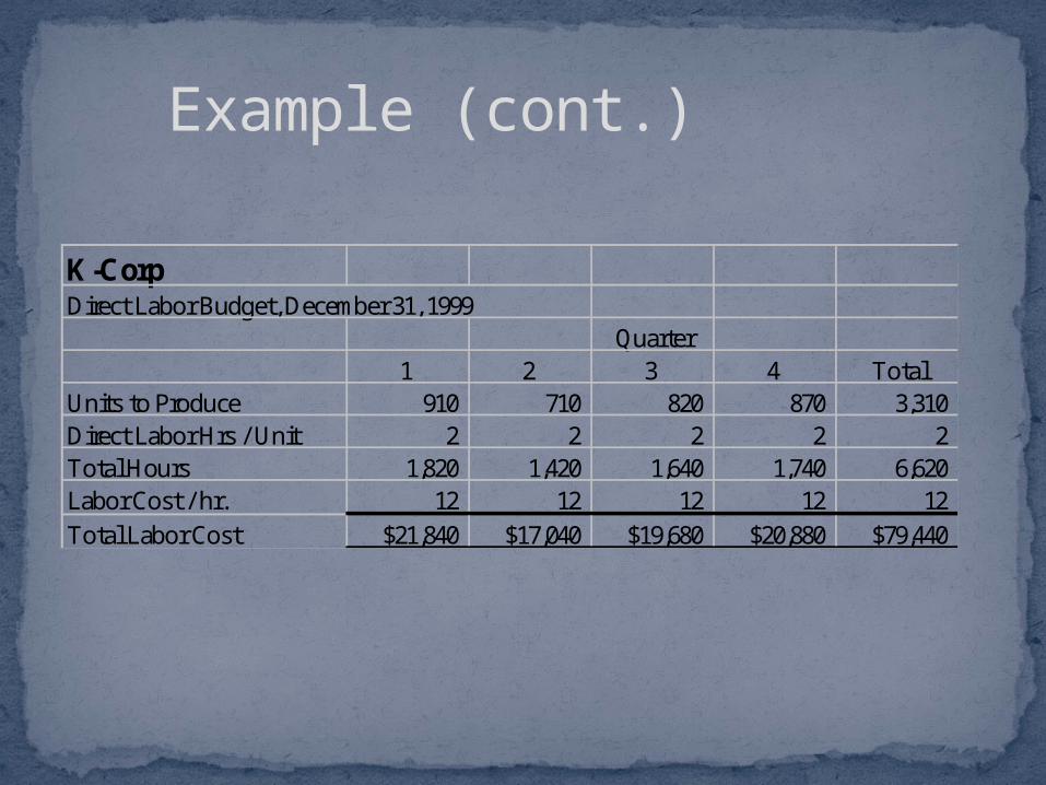
K-CorpDirect Labor Budget, December 31, 1999
Quarter1 2 3 4 Total
Units to Produce 910 710 820 870 3,310Direct Labor Hrs / Unit 2 2 2 2 2Total Hours 1,820 1,420 1,640 1,740 6,620Labor Cost / hr. 12 12 12 12 12Total Labor Cost $21,840 $17,040 $19,680 $20,880 $79,440
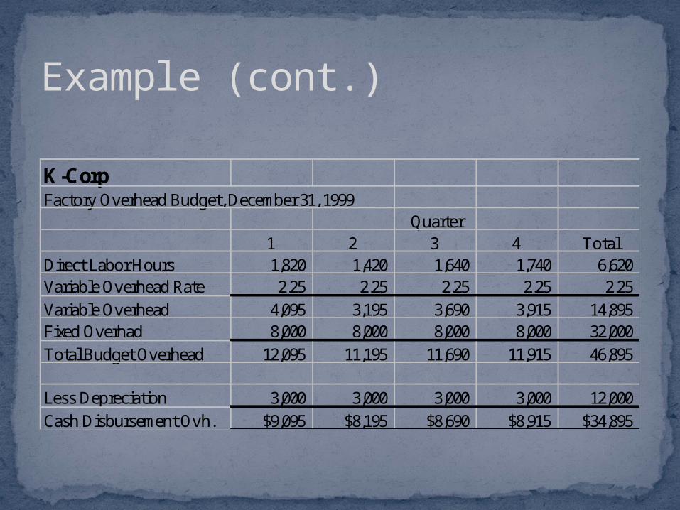
Example (cont.)
K-CorpFactory Overhead Budget, December 31, 1999
Quarter1 2 3 4 Total
Direct Labor Hours 1,820 1,420 1,640 1,740 6,620Variable Overhead Rate 2.25 2.25 2.25 2.25 2.25Variable Overhead 4,095 3,195 3,690 3,915 14,895Fixed Overhad 8,000 8,000 8,000 8,000 32,000Total Budget Overhead 12,095 11,195 11,690 11,915 46,895
Less Depreciation 3,000 3,000 3,000 3,000 12,000Cash Disbursement Ovh. $9,095 $8,195 $8,690 $8,915 $34,895
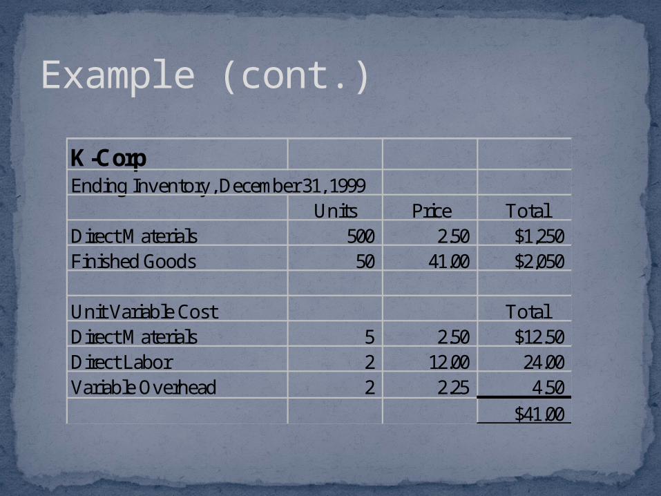
Example (cont.)
K-CorpEnding Inventory, December 31, 1999
Units Price TotalDirect Materials 500 2.50 $1,250Finished Goods 50 41.00 $2,050
Unit Variable Cost TotalDirect Materials 5 2.50 $12.50Direct Labor 2 12.00 24.00Variable Overhead 2 2.25 4.50
$41.00
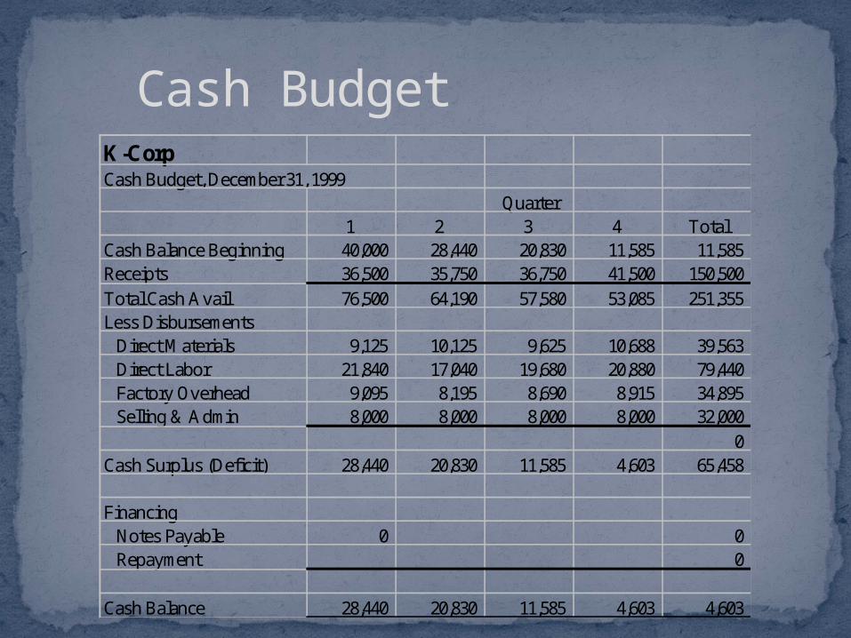
Cash BudgetK-CorpCash Budget, December 31, 1999
Quarter1 2 3 4 Total
Cash Balance Beginning 40,000 28,440 20,830 11,585 11,585Receipts 36,500 35,750 36,750 41,500 150,500Total Cash Avail 76,500 64,190 57,580 53,085 251,355Less Disbursements Direct Materials 9,125 10,125 9,625 10,688 39,563 Direct Labor 21,840 17,040 19,680 20,880 79,440 Factory Overhead 9,095 8,195 8,690 8,915 34,895 Selling & Admin 8,000 8,000 8,000 8,000 32,000
0Cash Surplus (Deficit) 28,440 20,830 11,585 4,603 65,458
Financing Notes Payable 0 0 Repayment 0
Cash Balance 28,440 20,830 11,585 4,603 4,603

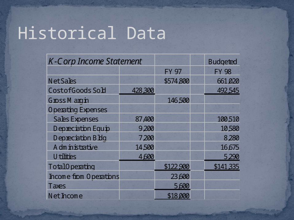
Historical DataK-Corp Income Statement Budgeted
FY 97 FY 98Net Sales $574,800 661,020Cost of Goods Sold 428,300 428,300Gross Margin 146,500Operating Expenses Sales Expenses 87,400 87,400 Depreciation Equip 9,200 9,200 Depreciation Bldg 7,200 7,200 Administrative 14,500 14,500 Utilities 4,600 4,600Total Operating $122,900 $122,900Income from Operations 23,600Taxes 5,600Net Income $18,000
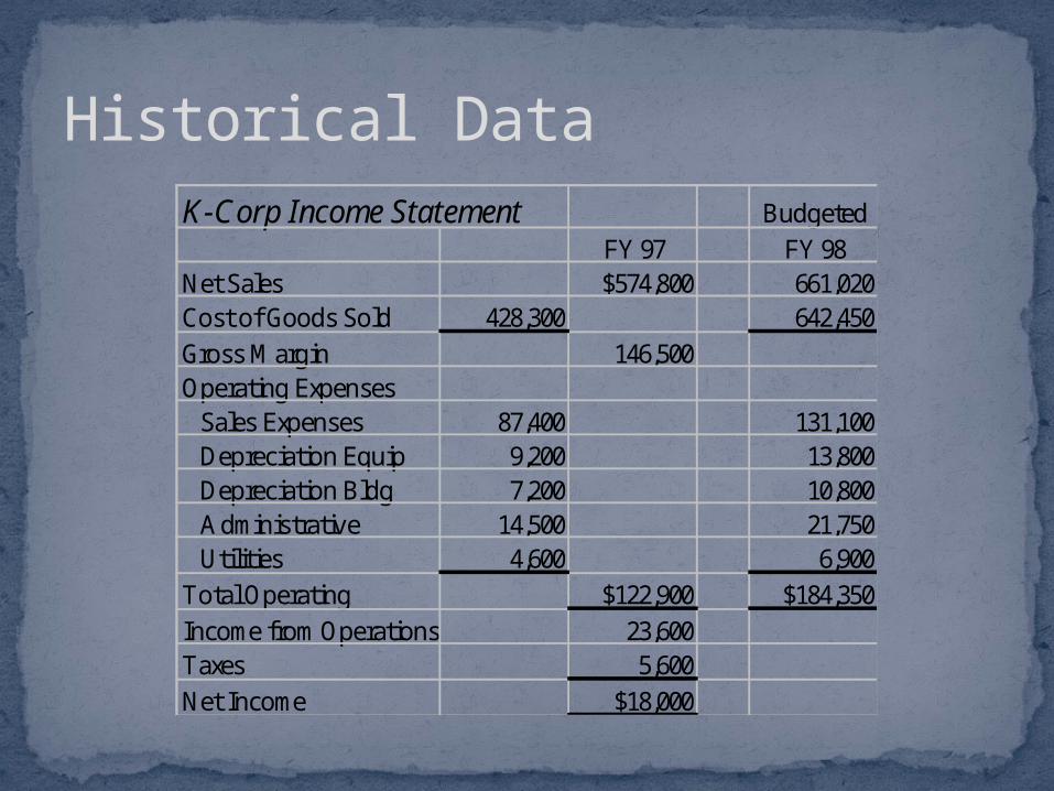
Historical DataK-Corp Income Statement Budgeted
FY 97 FY 98Net Sales $574,800 661,020Cost of Goods Sold 428,300 642,450Gross Margin 146,500Operating Expenses Sales Expenses 87,400 131,100 Depreciation Equip 9,200 13,800 Depreciation Bldg 7,200 10,800 Administrative 14,500 21,750 Utilities 4,600 6,900Total Operating $122,900 $184,350Income from Operations 23,600Taxes 5,600Net Income $18,000
Historical DataK-Corp Income Statement Budgeted
FY 97 FY 98Net Sales $574,800 661,020Cost of Goods Sold 428,300 492,545Gross Margin 146,500Operating Expenses Sales Expenses 87,400 100,510 Depreciation Equip 9,200 10,580 Depreciation Bldg 7,200 8,280 Administrative 14,500 16,675 Utilities 4,600 5,290Total Operating $122,900 $141,335Income from Operations 23,600Taxes 5,600Net Income $18,000

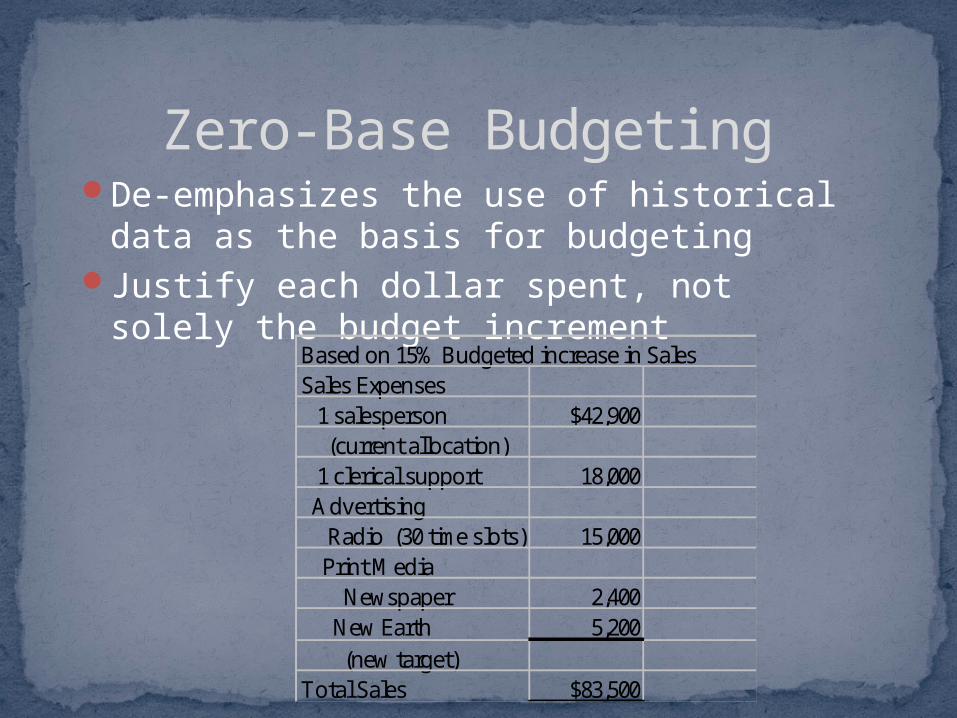
De-emphasizes the use of historical data as the basis for budgeting
Justify each dollar spent, not solely the budget increment
Zero-Base Budgeting
De-emphasizes the use of historical data as the basis for budgeting
Justify each dollar spent, not solely the budget increment
Zero-Base Budgeting
Based on 15% Budgeted increase in SalesSales Expenses 1 salesperson $42,900 (current allocation) 1 clerical support 18,000 Advertising Radio (30 time slots) 15,000 Print Media Newspaper 2,400 New Earth 5,200 (new target)Total Sales $83,500
Number of new customersProcess yieldSales calls per day per salesperson% late deliveriesrate of turnoverrate of absenteeism
Nonfinancial Parameters
Cost CentersManager responsible for develop a realistic
budget and controls expenditures to that budget
Profit CentersManager accountable for both revenue
generation and expense controlInvestment Centers
Manager has authority to commit investment resources
Responsibility Accounting

Budget VariancesSeptember Year - to Date
Budget Actual Variance Budget Actual VarianceSales $64,200 $67,300 $3,100 $635,580 $605,700 ($29,880)Operating Expenses Salaries 18,000 18,000 0 186,300 194,400 (8,100) Sales Commissions 14,000 14,700 (700) 126,000 119,070 6,930 Travel & Entertainment 5,000 4,400 600 45,000 41,580 3,420 Telephone 3,200 3,700 (500) 34,560 41,625 (7,065) Advertising 5,600 6,900 (1,300) 50,400 52,785 (2,385) Rent 3,500 3,500 0 34,650 28,350 6,300Total $49,300 $51,200 ($1,900) $476,910 $477,810 ($900)
Allocated Expenses Headquarters Sales 1,800 1,800 0 19,440 18,630 810 National Adv. 3,200 3,200 0 27,360 33,120 (5,760) Trade Shows 1,400 1,900 (500) 13,860 15,390 (1,530)Total $6,400 $6,900 ($500) $60,660 $67,140 ($6,480)

September Year - to DateBudget Actual Variance Budget Actual Variance
Sales $64,200 $67,300 $3,100 $635,580 $605,700 ($29,880)Operating Expenses Salaries 18,000 18,000 0 186,300 194,400 (8,100) Sales Commissions 14,000 14,700 (700) 126,000 119,070 6,930 Travel & Entertainment 5,000 4,400 600 45,000 41,580 3,420 Telephone 3,200 3,700 (500) 34,560 41,625 (7,065) Advertising 5,600 6,900 (1,300) 50,400 52,785 (2,385) Rent 3,500 3,500 0 34,650 28,350 6,300Total $49,300 $51,200 ($1,900) $476,910 $477,810 ($900)
Allocated Expenses Headquarters Sales 1,800 1,800 0 19,440 18,630 810 National Adv. 3,200 3,200 0 27,360 33,120 (5,760) Trade Shows 1,400 1,900 (500) 13,860 15,390 (1,530)Total $6,400 $6,900 ($500) $60,660 $67,140 ($6,480)
Positive (favorable) VariancesNegative (unfavorable) Variances
September Year - to DateBudget Actual Variance Budget Actual Variance
Sales $64,200 $67,300 $3,100 $635,580 $605,700 ($29,880)Operating Expenses Salaries 18,000 18,000 0 186,300 194,400 (8,100) Sales Commissions 14,000 14,700 (700) 126,000 119,070 6,930 Travel & Entertainment 5,000 4,400 600 45,000 41,580 3,420 Telephone 3,200 3,700 (500) 34,560 41,625 (7,065) Advertising 5,600 6,900 (1,300) 50,400 52,785 (2,385) Rent 3,500 3,500 0 34,650 28,350 6,300Total $49,300 $51,200 ($1,900) $476,910 $477,810 ($900)
Allocated Expenses Headquarters Sales 1,800 1,800 0 19,440 18,630 810 National Adv. 3,200 3,200 0 27,360 33,120 (5,760) Trade Shows 1,400 1,900 (500) 13,860 15,390 (1,530)Total $6,400 $6,900 ($500) $60,660 $67,140 ($6,480)
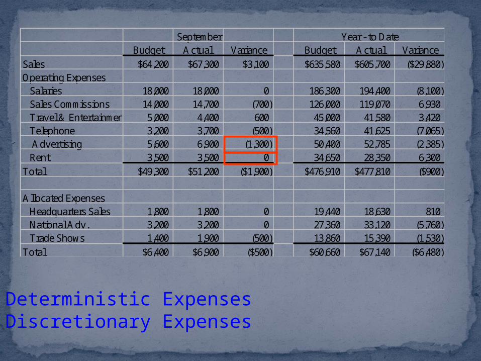
Deterministic ExpensesDiscretionary Expenses
September Year - to DateBudget Actual Variance Budget Actual Variance
Sales $64,200 $67,300 $3,100 $635,580 $605,700 ($29,880)Operating Expenses Salaries 18,000 18,000 0 186,300 194,400 (8,100) Sales Commissions 14,000 14,700 (700) 126,000 119,070 6,930 Travel & Entertainment 5,000 4,400 600 45,000 41,580 3,420 Telephone 3,200 3,700 (500) 34,560 41,625 (7,065) Advertising 5,600 6,900 (1,300) 50,400 52,785 (2,385) Rent 3,500 3,500 0 34,650 28,350 6,300Total $49,300 $51,200 ($1,900) $476,910 $477,810 ($900)
Allocated Expenses Headquarters Sales 1,800 1,800 0 19,440 18,630 810 National Adv. 3,200 3,200 0 27,360 33,120 (5,760) Trade Shows 1,400 1,900 (500) 13,860 15,390 (1,530)Total $6,400 $6,900 ($500) $60,660 $67,140 ($6,480)
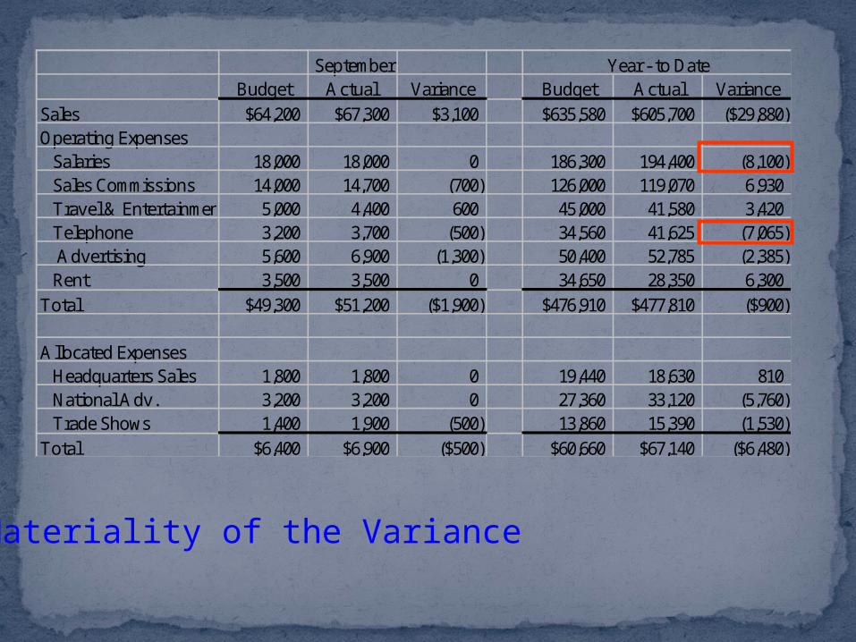
Materiality of the Variance

September Year - to DateBudget Actual Variance Budget Actual Variance
Sales $64,200 $67,300 $3,100 $635,580 $605,700 ($29,880)Operating Expenses Salaries 18,000 18,000 0 186,300 194,400 (8,100) Sales Commissions 14,000 14,700 (700) 126,000 119,070 6,930 Travel & Entertainment 5,000 4,400 600 45,000 41,580 3,420 Telephone 3,200 3,700 (500) 34,560 41,625 (7,065) Advertising 5,600 6,900 (1,300) 50,400 52,785 (2,385) Rent 3,500 3,500 0 34,650 28,350 6,300Total $49,300 $51,200 ($1,900) $476,910 $477,810 ($900)
Allocated Expenses Headquarters Sales 1,800 1,800 0 19,440 18,630 810 National Adv. 3,200 3,200 0 27,360 33,120 (5,760) Trade Shows 1,400 1,900 (500) 13,860 15,390 (1,530)Total $6,400 $6,900 ($500) $60,660 $67,140 ($6,480)
Timeliness
Date: 12-07-98
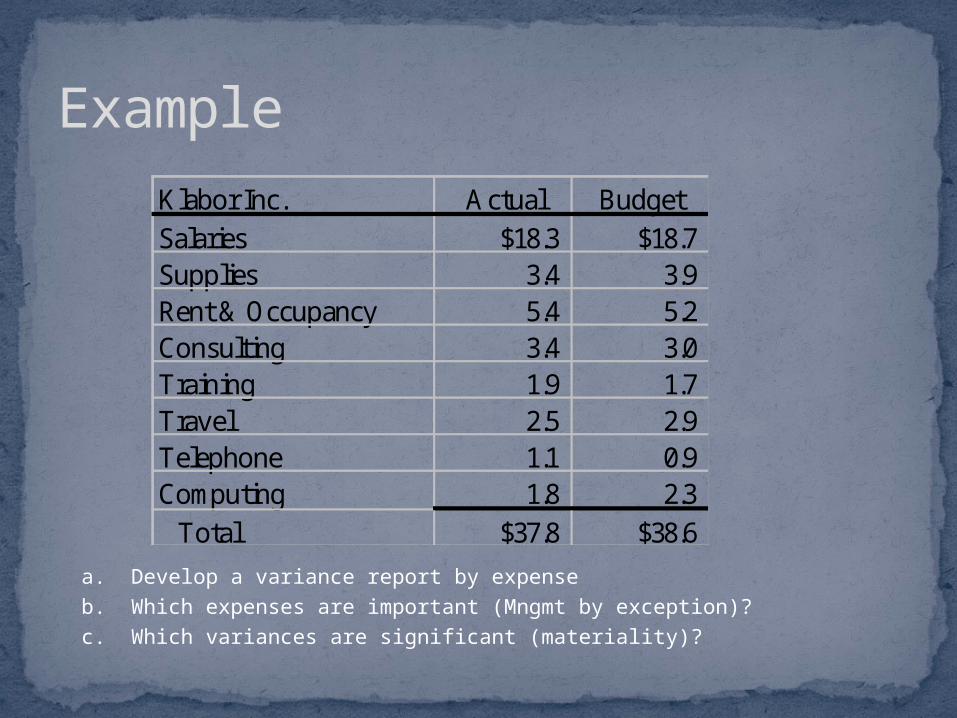
a. Develop a variance report by expenseb. Which expenses are important (Mngmt by exception)?c. Which variances are significant (materiality)?
ExampleKlabor Inc. Actual BudgetSalaries $18.3 $18.7Supplies 3.4 3.9Rent & Occupancy 5.4 5.2Consulting 3.4 3.0Training 1.9 1.7Travel 2.5 2.9Telephone 1.1 0.9Computing 1.8 2.3 Total $37.8 $38.6

Example
Klabor Inc. Actual Budget VarianceSalaries $18.3 $18.7 $0.4Supplies 3.4 3.9 $0.5Rent & Occupancy 5.4 5.2 ($0.2)Consulting 3.4 3.0 ($0.4)Training 1.9 1.7 ($0.2)Travel 2.5 2.9 $0.4Telephone 1.1 0.9 ($0.2)Computing 1.8 2.3 $0.5 Total $37.8 $38.6 $0.8