Jussi Nieminen

Brain activation in a complex stimulus

Faculty of Electronics, Communications and Automation

Thesis submitted for examination for the degree of Master ofScience in Technology.

12.4.2010

Thesis supervisor and instructor:

Prof. Jouko Lampinen

A’’ Aalto UniversitySchool of Scienceand Technology

Aalto-yliopistoteknillinen korkeakoulu

diplomityontiivistelma

Tekija: Jussi Nieminen

Tyon nimi: Aivoaktivaatio monimuotoisessa arsykkeessa

Paivamaara: 12.4.2010 Kieli: Englanti Sivumaara:7+47

Elektroniikan, tietoliikenteen ja automaation tiedekunta

Laaketieteellisen tekniikan ja laskennallisen tieteen laitos

Professuuri: Laskennallinen tekniikka Koodi: S-114

Valvoja ja ohjaaja: Prof. Jouko Lampinen

Tutkimuksessa luonnollisia olosuhteita jaljitellaan nayttamalla elokuvaa.Tallaisen arsykkeen aiheuttamaa yleista aivoaktivaatiota tutkitaan. Aivojenvasteita kyseiselle arsykkeelle selvitetaan. Riippumattomien komponenttienanalyysia (ICA) ja koehenkiloiden valisia korrelaatioita (ISC) kaytetaan datananalysointiin. ICA:sta saatujen komponenttien konsistenssia ja vaihtelevuuttatestataan. Koehenkiloiden samankaltaisuutta tutkitaan ISC:lla. Stabiilimmatkomponenttit aiheuttavia arsykkeita etsitaan elokuvasta, kuten tehdaan myosjoidenkin aivoalueiden ISC:lla.Elokuva Tulitikkutehtaan tytto naytettiin koehenkiloille, joiden aivojen aktiivi-suutta mitattiin toiminnallisella magneettikuvauksella (fMRI). Koehenkilot sai-vat vapaasti katsoa elokuvaa eika erillisia ohjeita annettu. FMRI:sta saatudata analysoitiin ryhma ISC:lla ja ICA:lla. ICA:n stabiilisuutta ja konsistenssiatestattiin ajamalla useita bootstrap ICA:ja. ISC laskettiin koko elokuvalle jaikkunoidulle datalle erikseen. Koko elokuva jaettiin viiteen taajuuskaistaan eritaajuuksien korrelaatioiden vertailua varten.ICA paljasti stabiileja komponentteja kuuloa ja nakoa prosessoivilla alueilla sekaparietaali alueella. ISC naytti synkronisaatiota paaosin samoilla alueilla. Datanjako taajuuskaistoihin paljasti aani ja kuulo alueiden hallinnan korkeilla taajuuk-silla. Aivojen etuosissa oli korrelaatiota matalilla taajuuksilla.

Avainsanat: fMRI, ICA, konsistenssi, ISC

Aalto UniversitySchool of Science and Technology

abstract of themaster’s thesis

Author: Jussi Nieminen

Title: Brain activation in a complex stimulus

Date: 12.4.2010 Language: English Number of pages:7+47

Faculty of Electronics, Communications and Automation

Department of Biomedical Engineering and Computational Science

Professorship: Computational engineering Code: S-114

Supervisor and instructor: Prof. Jouko Lampinen

Natural conditions are imitated by showing a movie as a stimulus. The commonbrain activity caused by this kind of stimulus is studied. The interest is to findwhat kind of responses brain gives to the stimulus. The independent componentanalysis (ICA) and the intersubject correlation (ISC) are used to analyze the data.Consistency and variability of the components revealed by group ICA are tested.Similarities between the subjects are tested by ISC. The stimuli causing the mostconsistent components are traced from the movie as is also done with ISC incertain brain regions.The beginning of the movie Tulitikkutehtaan tytto was shown to subjects whosebrain activity was recorded with functional magnetic resonance imaging (fMRI).The subjects could freely view the movie and no instructions were given. Theresulting data from fMRI was analyzed by group intersubject correlation andindependent component analysis. The stability and the consistency of ICA wastested by bootstrapping the data. Intersubject correlation was calculated to thewhole movie and windowed data separately. The whole movie was also divided to5 subbands to compare correlations in different frequencies.ICA revealed stable components in the auditory and the visual processing areasand in the parietal area. ISC showed synchronization mainly in the same regions.The subbands showed the dominance of the auditory and the visual processingareas in high frequencies. Frontal part of the brain had correlation in low frequen-cies.

Keywords: fMRI, ICA, consistency, ISC

iv

Preface

This work was done at the department of Biomedical Engineering and Computa-tional Science in Aalto University School of Science and Technology. I would like tothank my supervisor Professor Jouko Lampinen for the possibility to work in thisproject. I am grateful to Mikko Sams, Iiro Jaaskelainen, Juha Salmitaival, JuhaLahnakoski, Jukka-Pekka Kauppi and Jussi Tohka for supporting me in the study.Finally, I wish to thank all my coworkers, family and friends.

Otaniemi, 21.1.2008

Jussi Nieminen

v

Contents

Abstract (in Finnish) ii

Abstract iii

Preface iv

Contents v

Symbols and appriviations vi

1 Introduction 1

2 Theory 32.1 MRI . . . . . . . . . . . . . . . . . . . . . . . . . . . . . . . . . . . . 3

2.1.1 Definition of MRI . . . . . . . . . . . . . . . . . . . . . . . . . 32.1.2 Images . . . . . . . . . . . . . . . . . . . . . . . . . . . . . . . 62.1.3 BOLD fMRI . . . . . . . . . . . . . . . . . . . . . . . . . . . . 72.1.4 EPI . . . . . . . . . . . . . . . . . . . . . . . . . . . . . . . . 8

2.2 Preprocessing the brain images . . . . . . . . . . . . . . . . . . . . . 102.2.1 Motion correction . . . . . . . . . . . . . . . . . . . . . . . . . 102.2.2 Slice time correction . . . . . . . . . . . . . . . . . . . . . . . 102.2.3 Brain extraction . . . . . . . . . . . . . . . . . . . . . . . . . . 102.2.4 Spatial smoothing . . . . . . . . . . . . . . . . . . . . . . . . . 112.2.5 Temporal filtering . . . . . . . . . . . . . . . . . . . . . . . . . 122.2.6 Registration . . . . . . . . . . . . . . . . . . . . . . . . . . . . 122.2.7 Removal of artifacts . . . . . . . . . . . . . . . . . . . . . . . 13

2.3 Independent component analysis . . . . . . . . . . . . . . . . . . . . . 132.3.1 Basic principles of ICA . . . . . . . . . . . . . . . . . . . . . . 132.3.2 Probabilistic ICA model . . . . . . . . . . . . . . . . . . . . . 142.3.3 Group analysis . . . . . . . . . . . . . . . . . . . . . . . . . . 16

2.4 Intersubject correlation . . . . . . . . . . . . . . . . . . . . . . . . . . 172.4.1 Correlation . . . . . . . . . . . . . . . . . . . . . . . . . . . . 172.4.2 Intersubject Correlation Analysis . . . . . . . . . . . . . . . . 182.4.3 False Discovery Rate . . . . . . . . . . . . . . . . . . . . . . . 19

2.5 The previous studies of ICA and ISC . . . . . . . . . . . . . . . . . . 192.5.1 Consistency and variability of ICA . . . . . . . . . . . . . . . 21

3 Research material and methods 233.1 Subjects . . . . . . . . . . . . . . . . . . . . . . . . . . . . . . . . . . 233.2 Experiment . . . . . . . . . . . . . . . . . . . . . . . . . . . . . . . . 233.3 Data analysis . . . . . . . . . . . . . . . . . . . . . . . . . . . . . . . 23

3.3.1 Preprocessing . . . . . . . . . . . . . . . . . . . . . . . . . . . 233.3.2 Intersubject correlation . . . . . . . . . . . . . . . . . . . . . . 243.3.3 Independent component analysis . . . . . . . . . . . . . . . . 25

vi

4 Results 264.1 Intersubject correlation . . . . . . . . . . . . . . . . . . . . . . . . . . 26

4.1.1 Whole data . . . . . . . . . . . . . . . . . . . . . . . . . . . . 264.1.2 Windowed data . . . . . . . . . . . . . . . . . . . . . . . . . . 294.1.3 Stimuli in the movie . . . . . . . . . . . . . . . . . . . . . . . 304.1.4 Comparison . . . . . . . . . . . . . . . . . . . . . . . . . . . . 35

4.2 Consistency of independent components . . . . . . . . . . . . . . . . 354.2.1 Clustering . . . . . . . . . . . . . . . . . . . . . . . . . . . . . 354.2.2 ICA . . . . . . . . . . . . . . . . . . . . . . . . . . . . . . . . 364.2.3 Temporal variability . . . . . . . . . . . . . . . . . . . . . . . 36

4.3 Comparison of ICA and ISC . . . . . . . . . . . . . . . . . . . . . . . 42

5 Discussion 435.1 The study . . . . . . . . . . . . . . . . . . . . . . . . . . . . . . . . . 435.2 ICA . . . . . . . . . . . . . . . . . . . . . . . . . . . . . . . . . . . . 435.3 ISC . . . . . . . . . . . . . . . . . . . . . . . . . . . . . . . . . . . . . 435.4 Future research . . . . . . . . . . . . . . . . . . . . . . . . . . . . . . 44

vii

Symbols and appriviations

Symbols

w0 Larmor frequency gyromagnetic ratioB0 external magnetic fieldM0 net magnetization�f flip angleB1 strength of the RF pulsetp duration of the pulseG gradient fieldB magnetic fieldS(t) MR signal measured by an antennaT relaxation timek(t) k-spaceS(x, y) intensity in a pixelf(x, y, z) three dimensional Gaussian kernelx random vector of the observed valuesa attenuations random vector of the sourcesA mixing matrixz observed valueW inverse of the mixing matrixΣi noise covariance matrix�2 covarianceRx covariance matrixX voxel-wise prewhitened datap number of observationsq number of sourcesQ square matrix� Gaussian variable of zero mean and unit varianceF nonquadratic function� coefficient� mean� variancer correlation� thresholdp probabilityV number of true null hypothesispi p-value of the test iC correlation matrixk threshold valued longest acceptable path

viii

Appriviations

MRI magnetic resonance imagingfMRI functional magnetic resonance imagingNMR nuclear magnetic resonanceICA independent component analysisISC intersubject correlationGISC group intersubject correlationRF radio frequencyFID free induction decayTR repetition timeGE gradient echoSE spin echoTE echo timeBOLD blood oxygenation level dependentHDR hemodynamic responseEPI echo planar imagingDOF degrees of freedomMNI Montreal neurological institutePICA probabilistic independent component analysisPCA principal component analysisALS alternating least squaresFWE familywise error rateFDR false discovery rate

1 Introduction

The brain is one of human’s most important organs. Many studies for understand-ing how the brain works have been done over last decades. The brain controlsalmost every part of the human body. Actually the brain commands our everydaymovements and behavior. The interest of understanding functions of the brain istherefore understandable.

Brain’s responses to outside stimuli have been studied in different ways. Earlierthe stimuli have been simple sounds or pictures. These very controlled studies haveshowed which regions of the brain corresponds to auditory, visual or memory relatedstimuli. Nowadays studies have moved towards more naturalistic stimuli where thestimuli are related more closely to everyday life. This way it is possible to modelbrain in everyday events. One of the novel approaches is called neurocinematics. Inneurocinematics a movie is presented as a stimulus which is clearly more naturalthan still pictures or beep sounds.

New techniques for observing brain activity has been developed allowing theuse of better methods in brain studies. In functional magnetic resonance imaging(fMRI) changes in blood oxygenation level are measured revealing which regions ofthe brain are active at a particular time point. Images can be taken at 2 secondintervals revealing accurately the changes in the brain.

The object of the study is to find brain responses common to most of the subjects.The consistency of independent component analysis (ICA) is tested and stimuli caus-ing the consistent components are tried to be found from the movie. Correlationsbetween subjects during the movie watching are calculated to find which regionshave synchronization. To recognize the stimuli in the movie the correlations arealso calculated in shorter clips. Besides the study better understanding of the usedmethods should be achieved which can be utilized in forthcoming studies.

Experiment’s setup corresponds to the studies of Hasson et al.[1], Bartels andZeki[2] and Jaaskelainen et al.[3] where they viewed a movie that subjects couldfreely watch. A movie Tulitikkutehtaan tytto is shown to 12 subjects whose brainactivity is recorded with fMRI. The resulting data is analyzed by the intersubjectcorrelation (ISC) and the independent component analysis (ICA). The stability andconsistency of ICA is tested by bootstrapping the data. The results of ICA and ISCare also compared.

The intersubject correlation is counted for every subject pair. One common valueis formed from the subjects’ correlations. The data is divided to 5 subbands and itis also windowed to 71 clips. The synchronizations are counted for the whole datain every band separately and in full band for the windowed data.

Hypothesis is that the auditory and the visual processing areas of the brainhave strong correlations over the whole movie in full band. These areas should alsodominate in higher frequencies where frontal areas should have correlation only inlower frequencies. The correlations in different parts of the brain at different timepoints are expected to be found as the auditory processing areas should be activewhen there is speech in the movie and the visual processing areas should have higheractivation during visual stimuli.

2

The consistency of the found independent components is examined by bootstrap-ping group ICA. Also spatial and temporal variability of the independent compo-nents are examined. Here it is assumed that some very stable components causedby the real stimuli and some artifacts will be found. Finally these two methods toanalyze fMRI are compared and their advantages and disadvantages are discussed.

In Chapter 2 the basics of the functional magnetic resonance imaging are gonethrough. Also preprocessing steps for fMRI data are introduced and two analysismethods the independent component analysis and the intersubject correlation areexplained. Finally previous studies are discussed. The experiment setup and theused analysis methods are explained Chapter 3. The results of ICA and ISC arepresented in Chapter 4. Chapter 5 contains the discussion of the study.

3

2 Theory

2.1 MRI

Magnetic Resonance Imaging (MRI) is a medical imaging technique which produceshigh quality images of the human body. It is used in neurological, oncological andmusculoskeletal studies. MRI is based on nuclear magnetic resonance (NMR), whichwas first discovered in 1945 by Edward Purcell and independently by Felix Blochand Robert Pound. The first MR image was published in 1973.[4]

2.1.1 Definition of MRI

In MRI the interests are nuclei in human body. Nuclei consist of protons andneurons. Often a hydrogen atom is used in MRI because it is abundant in all tissuetypes. Its nucleus consists of one positively charged proton. A proton spins on itsown axis generating a magnetic field known as magnetic moment. The spinningbehavior of the hydrogen atom is quite simple compared to heavier atoms whichfavors its use in MRI.[4]

In addition to the spinning nuclei a strong magnetic field is needed to performMRI. This magnetic field affects the hydrogen nuclei in human body. Normallynuclei are randomly aligned. When a strong magnetic field is generated the nucleialign about with the direction of the field. They still experience torque which makesthem precess around direction of the external magnetic field. This is called Larmorprecession. It is proportional to the magnetic field given as Larmor frequency

w0 = B0 (1)

where is the gyromagnetic ratio and B0 is the external magnetic field.[4]Protons can align parallel or anti-parallel in the field neutralizing each other.

Still the parallel state is slightly favored. The magnetic moment vectors are evenlyspread out because the protons are all out of phase with each other. The sum of allmagnetic moments is aligned exactly with the main field B0 and it is called the netmagnetization M0.[4]

M0 is much smaller (1�T ) than B0 (1T ) so it can not be yet measured. Tomeasure M0 a 90o radio frequency (RF) pulse is used. RF frequency must be theLarmor frequency. M0 moves away from B0 as long as RF is switched on. The flipangle will be

�f = B1tp (2)

where B1 is the strength of the RF pulse and tp is duration of the pulse. RF signalalso brings all the spins into phase coherence.

After the RF pulse M0 is measured by detecting the voltage it induces in areceiver coil. The coil sees a magnetic field which induces a voltage varying at theLarmor frequency. The signal is called Free Induction Decay (FID). FID is nevermeasured directly instead echoes are created and measured. Right after RF pulse isswitched off nuclei realign their M0 so that it is parallel to B0. This measurement

4

is processed to obtain MR images. The time between two excitation pulses is calledrepetition time (TR).[4]

There are two types of echoes gradient (GE) and spin echoes (SE). In GE theexcitation pulse is used to create a smaller flip angle �f than 90 degrees. A negativegradient lobe is applied right after the excitation pulse causing rapid dephasing ofthe transverse magnetization. Then a positive gradient is applied which reversesthe magnetic field gradient. After a certain time gradients will come back into thesame phase making a gradient echo. This time is called echo time (TE). In SE spinsare left to dephase a certain time after a 90 degree RF pulse. After a time T a 180degree pulse is used to flip the spins around their axes. All the spins will come backto the starting phase creating the spin echo. This will happen at time 2T after thefirst RF pulse. The spin echo is illustrated in figure(1).[4]

Figure 1: SE where in B a 90 degree pulse is applied and in E a 180 degree pulseflips the spins[5]

When the RF signal is switched off protons start to realign back to their equi-librium position. This is called relaxation time. The protons lose energy that theyabsorbed from the pulse during the relaxation. M0 parallel to B0 starts to recoverand it is called T1 recovery. The time when M0 has recovered 63% of its equilibriumvalue is called the relaxation time T1. Also a dephasing of the spins following theirphase coherence happens during this time. The vector sum of the magnetic momentsand also the measured FID decay. This process is called the spin-spin relaxation.The time when the transverse magnetization drops to 37% of it initial value is thespin-spin relaxation time T2. In human body T1 always takes longer time than T2.[4]

An image still cannot be created from a MR signal detected by the static mag-netic field and the radio frequency coil. Gradient coils are used to get the spatialinformation needed for constructing MRI. A gradient coil causes the MR signal tobecome spatially dependent. The coil changes the main magnetic field so that itsstrength differs at different locations. A magnetic field that increases in a spatialdirection is created by a gradient coil making the recovery of the spatial informationeasy. The spatial directions x and y are going perpendicularly and z parallel to themain field.[6]

5

The Bloch equation describes the change in the net magnetization

dM

dt= M ×B +

1

T1(M0 −Mz)−

1

T2(Mx −My). (3)

The longitudinal magnetization

Mz(t) = M0(1− e−t/T1) (4)

and the transverse magnetization

Mxy(t) = Mx(t) +My(t)i = Mxy0e−t/T2e−iwt (5)

can be calculated from the Bloch equation where

Mx(t) = −M0e−t/T2 coswt (6)

My(t) = M0e−t/T2 sinwt. (7)

Now the magnetic field depends on the static field B0 and the gradient fields G.

B(t) = B0 +Gx(t)x+Gy(t)y +Gz(t)z (8)

The MR signal measured by an antenna can be expressed as the summation of signalfrom every voxel

S(t) =

∫x

∫y

∫z

Mxy0(x, y, z)e−t/T2e−iw0te−i ∫ t0 Gx(t)x+Gy(t)y+Gz(t)zdtdxdydz. (9)

Modern scanners demodulate the detected signal with the resonance frequency w0

so term e−iw0t can be removed. Also term e−t/T2 can be removed because it does notaffect the signals spatial location only the magnitude.[6]

Often 2D-imaging is used where the Gz gradient and the excitation pulse aresimultaneously applied allowing selection of the defined slice. Only the spins in theslice are tuned to match the frequency of the excitation pulse. Interleaved sliceacquisition, where for example 10 slices are excited in order 1, 3, 5, 7, 9, 2, 4, 6, 8,10, is used to avoid the effect of the previous excitation pulse. The magnetizationof an individual voxel within a slice is

M(x, y) =

∫ z0+△z/2

z0−△z/2Mxy0(x, y, z)dz (10)

where z0 is the centre of the plain. After the slice selection the magnetization isdependent only on x and y. A spatial frequency space the k-space is adopted tomake it easier to understand the relation between S(t) and the object to be imagedM(x, y). A transform

kx(t) =

2�

∫ t

0

Gx(�)d� (11)

6

ky(t) =

2�

∫ t

0

Gy(�)d� (12)

is applied. The MR signal from equation (9) becomes

S(t) =

∫x

∫y

M(x, y)e−i2�kx(t)xe−i2�ky(t)ydxdy. (13)

The gradients Gx and Gy are applied for encoding of the spatial locations. Everyvoxel in the slice gets a unique frequency. The transverse magnetization is repre-sented in the k-space. Gy is turned on before the data acquisition accumulating acertain amount of phase offset. During the data acquisition Gx is turned on chang-ing the frequencies of the spins. Each voxel is collected in a slightly different timepoint. Collection of the data is called filling the k-space. Finally the MR image is re-constructed from the k-space using the inverse Fourier transform. Also 3D-imagingis used mostly in anatomical scans. There two phase gradients and one frequencygradient are used.[6]

2.1.2 Images

MR images are produced using pulse sequences. The sequence contains radiofre-quency pulses and gradient pulses. Images are named depending on which T1 or T2relaxation time is used. Here are few images listed.[4]

T1-weighted MRI

GE or SE signal is used in T1-weighted MRI with short TE and TR. Scan can berun very fast due the short repetition time TR. T1- weighted images have a goodcontrast. They are usually used as anatomy pictures because different tissues aredistinguished clearly. Fat is bright, water is grey and fluids are dark.[4]

T2-weighted MRI

SE is used in T2-weighted MRI. SE has long TE and TR. Here fluids are bright andwater- and fat-based tissues are darker.[4]

T2*-weighted MRI

In T2*-weighted MRI scans GE sequence is used with long TE and TR. This increasescontrast when measuring venous blood. Fluids are bright and other tissues are greyin T2*-images.[4]

7

Figure 2: The T2*-weighted image on the left and the T1-weighted image on theright

2.1.3 BOLD fMRI

The blood oxygenation level dependent (BOLD) functional MRI is a MRI methodwhich measures the level of blood oxygen in different parts of the brain. It is based ondifferent magnetic properties of deoxygenated and oxygenated hemoglobin. Deoxy-genated hemoglobin is paramagnetic while oxygenated hemoglobin is diamagnetic.When a human detects a stimulus it causes neural activity in his brain. An activeneuron uses more energy than an inactive neuron. The need of energy causes anincrease of blood flow that delivers the primary energy sources glucose and oxygento the active neurons.[6]

T2*-imaging is used in BOLD fMRI. Introduction of an object with magneticsusceptibility into a magnetic field causes spin dephasing. This will result decayin the transverse magnetization which depends on T2*. High oxygenated bloodshould show more MR signal and low oxygenated blood should show less. Thesedifferences and changes can be measured by MR imaging. The change in MR signalcaused by neural activity is called the hemodynamic response (HDR). There is a lagin HDR compared to the neuronal events. As neuronal responses occur in tens ofmilliseconds HDR can be seen in 3-6 seconds.[6]

After the neural activity there is lack of oxygen because it is extracted by theactive neurons. This causes an increased inflow of oxygenated blood. More oxy-genated blood is supplied than is extracted decreasing the amount of deoxygenatedhemoglobin in blood causing a decrease in signal loss due the T2* effect. Whenmonitoring an active voxel by BOLD fMRI increase of neural activity can be seenafter 2 seconds and the peak of activity is reached in about 5 seconds. After the peaksignal decreases below the baseline and remains there a short period of time. This is

8

known as the poststimulus undershoot. If multiple consecutive stimuli happen theamplitude of the BOLD signal remains higher during the stimuli.[6]

BOLD fMRI is used to study quick changes in the brain. It is applied in cognitiveneuroscience in defining networks, understanding mechanisms and finding the corre-lation between brain and behavior. It can be helpful in medical science in mappingdamaged areas of the brain and testing drugs.[7]

2.1.4 EPI

Understanding the function of the brain requires fast acquirement of the images.In the echo planar imaging (EPI) the k-space is filled using a single excitation andrapid gradients[6]. EPI is a fast method to form a complete image from a singledata sample. The data is collected to the k-space and after that transformed to animage by Fourier-transform. The 3D-image is collected one slice at the time. InEPI first a RF signal is sent. After RF signal a read signal and a phase signal aresent. This is illustrated in figure(3) where the k-space is covered in two segmentsand Gx is the read signal and Gy is a phase signal. The k-space can also be coveredin more segments. EPI basically reads one row at a time and then jumps to a nextrow. This is illustrated in figure(4), where a two shot interleaved EPI is used.[7]

These images usually have poor resolution because of the small acquisition timerequired. Their anatomical contrast is also poor because they are tuned to highlightphysiological changes. These images can be taken in less than one second and aretherefore suitable for fMRI when blood oxygen changes are monitored.[8]

Figure 3: the RF, the read and the phase signals[9]

9

Figure 4: The two shot interleaved EPI[10]

10

2.2 Preprocessing the brain images

After MRI measures the brain data will be preprocessed. The preprocessing stepsare made to remove artifacts from the brain images and to make the subjects’ brainscomparable in the future statistical analysis. The preprosesecing steps convert theraw MRI data into images that look like brains. These steps, after the k-space datais reconstructed into a 3D-image, are shortly explained in this section.[7]

2.2.1 Motion correction

People should stay still in MRI scanner when brain activity is measured. Howeverwhen the measure takes several minutes muscles get tired and little motion is manda-tory. These moves affect the pictures so that after a movement the same part of thebrain appears in different voxel as it was before the movement. When processes ina certain area of the brain, for example in a voxel, are explored for the whole seriesof the measurements the accidental motion moves the monitored part to a differentvoxel. This can be prevented by the motion correction and it is very important forstructural and functional brain image analysis. The motion also creates artifact todata which can be separated by the motion correction from the real activation.[8]

In the forthcoming statistical analysis it is assumed that the location of a givenvoxel within the brain does not change over time. This is why the motion must beestimated and corrected. Normally with fMRI a reference image is selected fromwithin the series and other images are registered to that selected fixed image.[8]

2.2.2 Slice time correction

A fMRI picture is taken during the time of TR. The picture is collected one slice atthe time meaning that the first slice will be taken almost one TR before the last slice.When TR is 2 seconds the gap is big between the first and the last slice. Here theslice time correction can be used to correct the slightly different time taken slices torespond to the wanted time. In 2 seconds a lot of things can happen in the brain soit is important to remember that different slices do not exactly correspond to eachother. Also the future analysis assumes that the slices are collected at the sametime. Slices can be taken in regular up (1, 2, 3, . . . , n), regular down(n, n-1, . . . , 1)or interleaved order (2, 4, 6, . . . , n, 1, 3 ,5 , n-1). It is necessary to know in whichorder the slices of the image where taken to succeed in the slice time correction.

2.2.3 Brain extraction

Functional MR images often contain little and high resolution MR images containa lot of non-brain tissue. There are fat, the skull, the muscles, the eyeballs etc.besides the brain. The idea of the brain extraction is to remove these non-braintissues. The removal is important for the registration and the future analysis to besuccessful. The brain extraction will be done after the motion and the slice timecorrection.[11]

11

There have been three main methods for the brain extraction. To do it manuallythat can be done fairly accurately. However it’s time consuming to do the extractionmanually and sufficient training is required. Another way is thresholding with themorphology[12] where an intensity thresholding is applied. This is usually a semi-automated method where the user normally helps to choose the thresholds. Theaim is to separate image into the dark parts (scull, background), the light parts(eye balls etc.) and the less light part (brain tissue). The brain should be foundby finding the largest unbroken cluster which is not the background. The largestcluster almost always still contains some non-brain tissue via a thin strand of thebright voxels. These areas are disconnected with the morphological filtering wherethe links are eroded. The largest cluster is then chosen and extended back to sameextent as before erosion.[11]

The third way is to use the deformable surface models where a mesh is fittedto the brain surface in the image. There is normally a constraint that forces somesmoothness to the surface. The model is also fitted to a correct part of the image andthe surface is iteratively deformed from the starting point until the optimal solutionis found. This is probably the easiest of these three methods to automate.[11]

2.2.4 Spatial smoothing

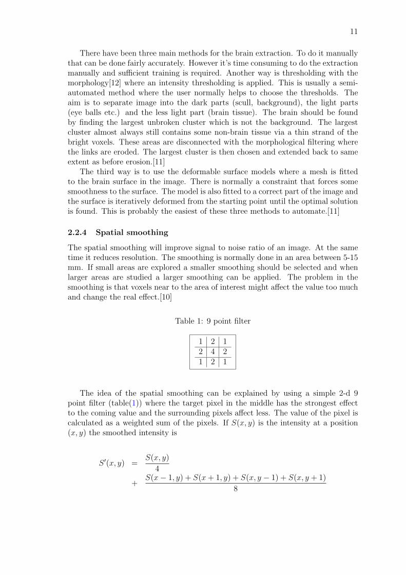
The spatial smoothing will improve signal to noise ratio of an image. At the sametime it reduces resolution. The smoothing is normally done in an area between 5-15mm. If small areas are explored a smaller smoothing should be selected and whenlarger areas are studied a larger smoothing can be applied. The problem in thesmoothing is that voxels near to the area of interest might affect the value too muchand change the real effect.[10]

Table 1: 9 point filter

1 2 12 4 21 2 1

The idea of the spatial smoothing can be explained by using a simple 2-d 9point filter (table(1)) where the target pixel in the middle has the strongest effectto the coming value and the surrounding pixels affect less. The value of the pixel iscalculated as a weighted sum of the pixels. If S(x, y) is the intensity at a position(x, y) the smoothed intensity is

S ′(x, y) =S(x, y)

4

+S(x− 1, y) + S(x+ 1, y) + S(x, y − 1) + S(x, y + 1)

8

12

+S(x− 1, y − 1) + S(x+ 1, y + 1)

16

+S(x− 1, y + 1) + S(x+ 1, y − 1)

16(14)

Normally some type of Gaussian kernel is applied in stead of the 9 point filter. Forexample a three dimensional Gaussian kernel might be applied

f(x, y, z) = exp(−(x2

2s2x+

y2

2s2y+

z2

2s2z)) (15)

where sx, sy and sz are the standard deviations.[10]

2.2.5 Temporal filtering

The temporal filtering will improve signal to noise ratio. It will remove long fre-quencies or low frequencies from the data often caused by the scanner or other partsof the body. Each voxel’s time series is smoothed separately in the Fourier domain.The filtering must be done with care so that the signal of interest will not be lost.For example there might be low drifts caused by the brain too.

2.2.6 Registration

Human brains differ in size and shape. The corresponding parts of each brain mightlocate in different voxels of the scanned images. To make the brains comparable toeach other and to define a spatial relationship a registration to a standard brain isused. This means transforming the brain to correspond a common template brain.[7]

The linear and the non-linear transformation are two common classes of thetransformation. In the linear transformation there are 12 or less degrees of freedom(DOF) and in the non-linear transformation there can be millions of DOF. In lineartransformation there are three translations, three rotations, three scaling and threeskew parameters one for each axel. Commonly the rigid body (6-DOF) includingtranslation and rotation, the similarity (7-DOF) including translation, rotation anda global scaling or the affine transformation (12-DOF) including all parametersare used. Only the translation and the rotation should be necessary for a goodregistration but in practice DOF is often increased to 12 or even the non-lineartransformation is used to get a better registration.[7]

The Talairach space from atlas of Talairach and Tournoux 1988 and the MontrealNeurological Institute (MNI) space are two commonly used spaces where the imagesare registered. The Talairach space is based on a single brain of a 60 years oldwoman. The MNI space is a combination of MRI scans on normal controls.

Registration for fMRI

The registration will be performed after the other preprocessing stages discussedearlier are done. Also non-brain structures from a structural image must be removed.Then there will be three registration stages to execute. At first the functional image

13

is registered to the subject’s structural image then the structural image is registeredto the template image. Finally these two transforms are combined. This process willbe performed to every measurement so that they will correspond to each other.[7]

2.2.7 Removal of artifacts

When brain activity is recorded with fMRI a problem with low signal to noiseratio is often encountered. In addition to the head motion there are other thingscausing artificial activation. Artifacts can be caused by the scanner, heart beator breathing. Many physiological components are of higher frequencies than TRand are aliased within fMRI signal[13]. These are therefore hard to remove usingfiltering. These components can be found by the independent component analysisthat maximizes independence. As the independent artifacts are found they can beremoved from the original data to make future analysis better. Some methods forremoving these artifacts have been developed by Thomas et al.[14],and Kochiyamaet al.[15], Perlbarg et al.[16]and Tohka et al.[17]

2.3 Independent component analysis

The independent component analysis (ICA) is a signal processing method which canseparate original signals from their mixed signals. When two people are speakingat the same time they produce two voice signals s1(t) and s2(t). If there are twomicrophones recording these voice signals two mixtures will be got of them

x1(t) = a11s1 + a12s2 (16)

x2(t) = a21s1 + a22s2 (17)

where a11, a12, a21 and a22 are parameters defining the attenuation of the originalvoice signals. ICA allows the estimation of aij based on the information of theirindependence. As aij is known the original signals can be separated from the mixedsignals.[18]

Originally ICA was used for problems like the previous one or closely related toit known as the cocktail-party problems. Later ICA has been found useful for brainresearch. ICA is a powerful method for unmixing linear mixtures of unknown inde-pendent sources[19]. It is nowadays used to separate signals in electroencephalogram(EGG) and fMRI studies.[18]

2.3.1 Basic principles of ICA

Instead of sums as in the equations 16 and 17 the vector-matrix notation will be used.Let x be a random vector whose elements are the observed values x1, x2, . . . , xm, ands is a random vector whose elements are the sources s1, s2, . . . , sn. A is a squaremixing matrix with elements aij. The mixing model can be written

x = As (18)

14

where x is a linear combination of different sources.[18]ICA is closely related to the blind source separation (BSS). The idea is to es-

timate the mixing matrix A and calculate its inverse W so that the independentsource values sn

s = Wx (19)

can be determined. The order of the independent components can not be deter-mined. The sources can be in different order in two tests with the same observedvalues. The resulting sources might also be multiplied by -1. However these donot matter in most applications. All independent components must be nongaussianexcept one because the mixing matrix A is not identifiable for Gaussian independentcomponents.[18]

To find the independent components gaussianity is minimized. A nongaussiancomponent gives a good approximation for an IC because the sum of two indepen-dent variables sn is always more Gaussian than the original variables. There aremany ways to minimize the gaussianity. Hyvarinen and Oja[18] write about kur-tosis, negentropy, minimization of the mutual information and maximum likelihoodestimation as ways to minimize the gaussianity.[18]

Normally there are two preprocessing steps in ICA centering and whitening. Inthe centering x is made zero-mean. In the whitening vector x is transformed linearlyso that its components are uncorrelated and their variance equal unity.[18]

2.3.2 Probabilistic ICA model

There are few problems in the ICA model. The mixing matrix A is assumed tobe square and there is no noise included to the model. These problems have beensolved by probabilistic ICA (PICA)[20]. PICA allows a nonsquare mixing processand assumes that data has some Gaussian noise

x = As+ �. (20)

The mixing matrix will be estimated from the data. PICA is specially optimizedfor fMRI data analysis. The idea is to decompose the data into independent mapswhich describe different activation patterns. ICA also separates artifacts from thereal data. ICA does not need a model for signal separation and that’s why it isuseful in brain research.[20]

In PICA there are different stages. At the first stages a signal-noise subspaceis estimated. This is done by employing probabilistic principal component analysis(PCA) [21]. Then the independent components are estimated from the subspaceby maximizing the non-gaussianity using a fixed-point iteration scheme[18]. Finallythe statistical significance of the components will be assessed. The ICA estimatesare transformed to Z-scores based on the estimated standard error of the residualnoise.[20]

In the model the noise covariance matrix Σi is assumed to be known. Thenthe data can be whitened with the respect of the noise covariance. In PICA it isassumed that noise and signal are uncorrelated and

15

Rx − �2I = AAt (21)

where Rx = ⟨xixti⟩ is the covariance matrix of the observation. Let X be thep ×N matrix of the voxel-wise prewhitened data vectors where p is the number ofobservations. The singular value decomposition of X is X = U(NΛ)

12Qt. If the

number of sources q is known we can estimate

AML = Uq(Λq − �2Iq)12Qt (22)

where Uq and Λq contain the first eigenvectors and eigenvalues of U and Λ and whereQ denotes the q × q orthogonal rotation matrix.[20]

After whitening data with respect to the noise covariance and projecting thetemporally whitened observations onto the space spanned by the q eigenvectors ofRx with the largest eigenvalues, the estimation of the mixing matrix A reduces toidentifying the square matrix Q. Then generalized least-squares is used for MLestimates

sML = (AtA)−1Atx (23)

�2ML =

1

p− q

l=q+1∑p

�l (24)

By iterating the estimates A and s and re-estimating the noise covariance from theresiduals � the model can be solved in the case of full noise covariance.[20]

The source distribution is assumed to be Gaussian and probabilistic PCA[21]can be used to estimate the number of sources q. To complete the estimation theorthogonal rotation matrix Q is optimized in the whitened space. Here a fixedpoint algorithm by Hyvarinen and Oja[18] is used that uses negentropy in order toestimate the non-Gaussian sources. The sources are catered by projecting the dataonto the individual rows of Q. The r’th source is estimated

sr = vtr(x) (25)

The source estimates are optimized by a contrast function

J(sr) ∝ ⟨F (sr)⟩ − ⟨F (�)⟩ (26)

where � is a Gaussian variable of zero mean and unit variance and F is a non-quadratic function[22]. The vector vtr is optimized to maximize J(sr) using theapproximate Newton method.[20][18]

Finally individual ICA-maps sr are converted into Z-statistic by dividing IC-maps by the estimate of the voxel-wise noise standard deviation. Gaussian mixturemodels are fitted to these Z-scores to find out the significance of each voxel. Thedistribution of the spatial intensity values of the rth Z-map is modeled by K mixturesof 1-dimensional Gaussian distributions[23]

16

p(zr ∣ �K) =K∑l=1

�r,lNzr [�r,l, �2r,l] (27)

where �K = [�K , �K , �K ] and �K ,�K ,�K are the vectors of the K mixture coefficients,means and variances. This model is fitted using the expectation-maximizationalgorithm[24] and an approximation to the Bayesian model evidence is used to findthe correct number of mixtures.

It is asumed that the first term in the mixture models the background noise.The posterior probability for activation is calculated by dividing the other mixturesby the whole distribution[25]

Pr(activation ∣ zr,i) =

∑Kl=2 �r,lNzr [�r,l, �

2r,l]

p(zr ∣ �K). (28)

Final PICA-components are formed using a certain significance level. The wholePICA process is illustrated in figure(5).[20]

Figure 5: pica[20]

17

2.3.3 Group analysis

The brain activity between different individuals differs from each other during themeasurement. However there might be some common patterns between all of the in-dividuals or at least maturity of them. To compare similarities between the subjectsa group analysis can be used. One method to compare similarities, where a stimulusis consistent between subjects, is the multi-session tensor-ICA which is derived fromthe Parrallel Factor Analysis[26].[27]

In tensor-ICA data is represented in 3D-array

xijk =R∑r

airbjrckr + �ijk (29)

where i = 1, . . . , I; j = 1, . . . , J ; k = 1, . . . , K and the dimensions are time, space andthe subjects. This is decomposed into three factor matrices A, B and C, time andthe components, space and the components and the subjects and the components.The problem can be solved using the Alternating Least Squares (ALS) by iteratingleast squares solution for

Xi.. = BΛ(ai)Ct + Ei.. i = 1, . . . , I (30)

X.j. = CΛ(bj)At + E.j. j = 1, . . . , J (31)

Xi.. = AΛ(ci)Bt + E..k k = 1, . . . , K (32)

where Λ(ai) is the R × R diagonal matrix where the diagonal elements are takenfrom the elements in row i of A.[27]

These can be alternatively expressed as a matrix products. For example equation(32) can be expressed

XIK×J = (C∣ ⊕ ∣A)Bt + E. (33)

Tensor-ICA directly estimates separate modes in the three domains. It does not treatall modes of the variation as equal. Tensor-ICA puts stronger statistical constraintson the spatial domain where a lot of data is available. The model is formulatedso that it includes the assumption of the maximally non-gaussian distribution ofthe estimated spatial maps. The algorithm has two stages. Estimate B from X byestimating M as the mixing matrix using PICA

XIK×J = MBt + E. (34)

and decompose the estimated mixing matrix M such that

M = (C∣ ⊕ ∣A) + E2. (35)

This is continued until convergence.[27]

18

2.4 Intersubject correlation

The intersubject correlation is a model-free technique where an activation of thereference subject is used to predict an activation of the other subjects. The pre-diction is done by calculating the correlation coefficient between the time coursesof the two subjects. When different subjects brain activity is compared with theintersubject correlation during a natural viewing there does not have to be anyprior design matrix or assumptions of the functional responses. The parametricmapping is based on the similarity in the blood oxygenation level dependent signalbetween the subjects[28]. Hasson et al.[1], Golland et al.[29], Jaaskelainen et al.[3]and Kauppi et al.[28] have used the intersubject correlation analysis to analyze fMRbrain images taken during watching movies.[1]

2.4.1 Correlation

Correlation measures the degree of statistical relationship between random variablesor observed data values. A familiar measure of the dependence between two variablesis the Pearson’s correlation coefficient

r =

∑ni=1[(xi − x)(yi − y)]√∑n

i=1(xi − x)2∑n

i=1(yi − y)2(36)

where x1, x2, . . . , xn and y1, y2, . . . , yn are the random variables and x and y are themeans of the random variables.

The Pearson’s correlation coefficient will give values between -1 and 1 reflectingthe linear relationship between the variables. The closer the value is to -1 or 1 thestronger the dependence as 0 tells that the variables are independent. Positive valuesmean a positive dependence and negative values reflect a negative dependence.

2.4.2 Intersubject Correlation Analysis

The intersubject correlation analysis is developed for processing natural stimuli ingroup fMRI data. The time series of the subjects’ brain activity are comparedvoxel-by-voxel basis with a chosen similarity criteria. Similarities are calculated tothe whole brain. In the intersubject correlation analysis tool[28] the fMRI timeseries are divided to frequency subbands and the same calculations are repeated forthem. The calculations are first done between every subject pair and from those asingle index is calculated which describes the total similarity.[28]

A wavelet filter bank is constructed using the stationary wavelet transform. TheJ-scale wavelet filter bank is built using the Daubechies 2 quadrature mirror functionpair in order to perform the frequency analysis. This way J+1 frequency subbandswill be obtained.[28]

The correlation is first calculated over every brain voxel between every pair

rij =

∑Nn=1[(si[n]− si)(sj[n]− sj)]√∑N

n=1(si[n]− si)2∑N

n=1(sj[n]− sj)2(37)

19

where N is a number of samples, si and sj are the time series of i’th and j’thsubject and si and sj are the corresponding means. Then the pairwise correlationsare averaged

r =1

(l2 − l)/2

l∑i=1

l∑j=2,j>i

rij (38)

to get a sigle index that gives group level information. The number of subjects isdenoted by l.[28]

The calculations are also done in shorter time frames in addition to the wholedata. The data is windowed to equally long time series each beginning a certain timestep after the previous one. The same time points can appear in many consecutivewindows if the time step is shorter than the size of the window. A time series fromthe number of the correlating voxels in the windows can be constructed. The voxelscan also be selected from a brain region of interest and only it can be explored. Thewindowing gives more accurate information of the synchronizations at the differenttime points. This can be used in finding the stimuli causing the dependencies inthe brain responses. It is easier to find the stimuli causing the correlations whenoverlapping windows are used.[28]

A voxel-wise permutation test similar to Wilson et al.[30] was performed to testthe signifigance of the results. Each subject’s time series were randomly circularlyshifted to calculate r statistic. The resulting p-values were corrected using FalseDiscovery Rate with independence or positive dependence assumption.[28]

2.4.3 False Discovery Rate

Brain images contain over 100,000 voxels. When thresholding 100,000 voxels at� = 5% threshold, 5000 false positives would be expected in null data and is thereforeinappropriate. The false positives must be controlled over all tests. The familywiseerror rate (FWE) has been the standard measure of the Type I errors in multipletesting. It is the probability of any false positives.[31]

Benjamini and Hochberg[32] introduced Bonferroni related method the false dis-covery rate (FDR) control which has a greater control than FWE. The Bonferroniinequality is a truncation of Boole’s formula[33]. It gives

pi =�0

V(39)

where V is the number of null hypothesis, �0 is the treshold and pi p-value of thetest i. However it did make no assumption on dependence between tests which nearvoxels in fMRI data have. FDR was proven to be valid under independence byBenjamini and Hochberg. Later Benjamini and Yekutieli[34] showed that the FDRmethod is valid also under dependence. FDR with the independence or positivedependence assumption has the form

pi ≤�0 ∗ iV

(40)

20

It is a step-up test which proceeds from the least to the most significant p-value. Thefirst that satisfies the equation implies that all smaller p-values are significant.[31]

2.5 The previous studies of ICA and ISC

There have been many neuroimaging studies where a same fixed stimulus is presentedfor different humans whose brain activity is monitored at the same time. Picturesare presented or sounds are created to make stimuli for brain. The tests have beenrestricted and therefore the possibility for an individual variation has been low.Recently studies have moved towards a more natural environment. For examplemovies are presented where brains receive different stimuli continuously. Subjectscan freely move their eyes and they might pay attention to different parts of thescene. Also connected plot and different characters create strong emotions. Bartelsand Zeki[2] and Hasson et al.[1] used movies to create more naturalistic stimuli.

Hasson et. al. used intersubject correlation analysis where voxels’ time coursesof one brain were used to predict the activity in other brains. Also the reverse-correlation method was applied. It uses the brain activation to find the stimuliin the movie. The time points of the activation in a particular part of the brainwhere located. The movie was then examined from these same time points to findthe stimuli that caused the activation in this particular region. They showed a 30minute segment of the movie ”The good, the bad and the ugly”. The movie wasassumed to give a much richer and complex stimulus than constrained visual stimuliin the laboratory.[1]

Hasson et. al. found out that the brains of the different individuals have atendency to act the same way during free viewing of the movie. Significant inter-subject correlations were found in the well-known visual and auditory cortices andalso in the high-order association areas. The reverse-correlation approach was usedto study the time courses of the face related posterior fusiform gyros and the build-ing related collateral sulcus. The highest peaks of both regions’ time courses werecompared to related frames of the movie. 15 of the 16 highest peaks in the fusiformgyros were associated with face images and 13 out of the 16 highest peaks of thecollateral sulcus were associated with scene images. These brain regions maintainedtheir selectivity under free viewing of the complex scenes.[1]

From regions that are typically not activated with these kind of stimuli Hassonet. al. studied areas where the intersubject correlation was significant. They foundregions that could be related to action in the movie for example a cortical regionlocated in the middle postcetral sulcus was connected to hand movements in themovie.[1]

Independent component analysis was first used for fMRI data by McKeown etal.[35]. Bartels and Zeki[2] showed a clip of the movie ”Tomorrow never dies” to8 subjects and monitored their brain activity during the movie. They used ICAto separate independent components from the data. They selected ICs whose mostsignificant voxels corresponded anatomically and which had significant intersubjectcorrelations. In almost every subject they found 10 ICs whose most significantvoxels corresponded across subjects. Most of these components were anatomically

21

located in the visual processing areas and the auditory areas. They found that thefunctional organization of the brain during natural conditions was preserved, ICAdetected voxels that belonged to different subdivisions and cortical subdivisions wereseparated to different ICs.[2]

Jaaskelainen et al.[3] studied emotions by viewing the movie Crash. fMRI wasmeasured during a free viewing of the movie. They calculated the intersubjectcorrelations which was high in many cortical and subcortical areas. Also manyprefrontal cortical areas were significantly correlated. They did also an ICA analysiswhich expose ICs from the primary visual areas V1, V2 and V5 but they could notfind clear events that caused those ICs. ICs that had a clear connection to the moviewere related to auditory activity. Two ICs showed activation when there was speechin the movie. However these ICs did not show activation when there was music ornon-speech sounds in the movie.[3]

Kauppi et al. divided the fMRI data from the movie Crash to subbands. Acommon value for the group intersubject correlation was calculated to the full bandand every subband separately. Correlation was found in the auditory and the visualprocessing areas in high frequencies. Low frequencies showed correlation also infrontal part of the brain.[28]

2.5.1 Consistency and variability of ICA

Solution in ICA can slightly change each time the method is applied. A statisticalstudy can be done to find how stable the method and different ICs are. This willreveal the importance of the resulting components. It also reveals how different com-ponents are divided in different analysis. Jarkko Ylipaavalniemi presents a methodin his master’s thesis which measures stability of the independent components[36].He has used bootstrapping to measure variability of the independent components.

At first multiple ICAs are run. Then the resulting independent components areclustered spatially. From those clusters the spatial variability can be measured.Also the temporal changes between the spatially corresponding components can beseen.[36]

ICA is run multiple times and the results are concatenated together

Aall = [A1 ∣ A2 ∣ . . . ∣ An] (41)

where each column of Aall defines an independent component and matrix An definesthe mixing matrix of the n’th run. Before the estimates are clustered they are madezero mean and unit variance. The similarity of the normalized ICs is measured bycalculating the correlation of each IC pair which forms a correlation matrix

C ∝ ATA. (42)

In order to find significant similarities each element of the correlation matrix C isthresholded with a value k

cij =

{1, if ∣cij∣ > k0, if ∣cij∣ < k

22

where all interesting correlations get the value one and others get the value zeroforming a binary correlation matrix C.[36]

The matrix shows the relation between adjacent estimates ai and aj which willbe put to the same cluster. If aj is also related to ak but ak is not straight related toai it is still recommended to put ai and ak to the same cluster. These longer pathscan be found by raising the correlation matrix to a power

R = Cd (43)

where d defines the longest acceptable path.[36]The ICs are clustered with a method where all ICs that have rij > 1 are sorted in

descending order according to cij. Then the list is gone through. If linked estimatesai and aj do not belong to a cluster a new cluster is created. If either of thecomponents belongs to an existing cluster the other one is added there too. If bothbelong to an existing cluster nothing is done.[36]

There are also other ways to cluster ICs. One is explained here. The group ICAis first run with all subjects. Then N numbers of bootstraps are run with the samesubjects. The resulting ICs from the original run are gone through from the firstto the last and from all bootstrap runs corresponding components are found andput to the same cluster. If the best fitting bootstrap component is already occupiedby another IC of the original run the second best component will be tried. This iscontinued until a free component is found. From the components in one cluster anIC estimate is calculated as weighted average of the components using correlationto the old estimate as a weight. In the first step the original run is used as the oldestimate and later the previous estimate is applied.

The bootstrap runs are gone through in an ascending order and all componentsin a run will be tested in an ascending order. If a component fits better to anotherestimate and changing position of this component with the component belonging tothe other cluster makes the model better the positions will be changed otherwisenothing is done. After a change the estimates are updated. When all runs are gonethrough the examination will move back to the first run. This will be continueduntil convergency.

23

3 Research material and methods

3.1 Subjects

Twelve subjects participated to the study. To make sure that the subjects did nothave any obstacles for participating to fMRI study they filled a safety questionnaire.An approval to the study was obtained from the subjects. All subjects were Finnishbecause the audio track of the movie was in Finnish.

3.2 Experiment

A 23 minute clip from the beginning of the movie Tulitikkutehtaan tytto was shownto the subjects. The subjects were instructed to watch the movie freely like in thestudies of Hasson et al.[1] and Bartels and Zeki[2]. The brain activity of the subjectswas measured with fMRI during the movie.

The subjects removed all metallic objects before the scanning and a metal de-tector was used to secure the subjects safety and to prevent noise signals in fMRI.The subjects lay in a MRI scanner. The movie was projected onto a translucentscreen which was viewed through an angled mirror. The auditory track of the moviewas presented through auditory tubes and earphones. Headsets were also worn toprevent the noise of the scanner. The subjects were instructed to stay still duringthe scanning in order to avoid motion artifacts.

Functional brain images were taken with a 3.0 T GE Signa Excite MRI scanner(GE Medical Systems, USA) using a quadrature 8-channel head coil in the AMICenter at the Helsinki University of Technology. A total of 689 volumes of EPI werescanned. There are 29 slices in an EPI sequence with the repetition time (TR) of2000 ms and the echo time (TE) of 32 ms. Images were obtained in axial orientation(thickness 4 mm, between-slices gap 1 mm, in-plane resolution 3.4 mm x 3.4 mm,voxel matrix 64 x 64, flip angle 90∘).

Also an anatomical T1-weighted inversion recovery spin-echo volume was ac-quired (TE 1.9 ms, TR 9 ms, flip angle 15∘). The T1 image acquisition used thesame slice prescription as did the functional image acquisition, except for a denserin-plane resolution (in-plane resolution 1 mm x 1 mm, matrix 256 x 256).

3.3 Data analysis

The fMRI data was first preprocessed. After preprocessing the intersubject corre-lation analysis and the independent component analysis were run. These processesare explained here.

3.3.1 Preprocessing

FSL[37] software was used for preprocessing the EPI images. First MCFLIRT wasused to remove the effect of head motion. Then the non-brain structures wereremoved with BET. BET was run to the motion corrected images resulting a singleimage. The motion corrected images were then masked with this image. A 10 mm

24

spatial smoothing was applied and the data was high pass filtered with 100s cutoff.600s high pass filter was used for bootstrapping data. In order to make comparisonof the different brains possible images were registered to the MNI template image.This was done by first registering the images to their structural images using 6 DOFand then registering the resulting images to MNI152 T1 2mm brain standard brainusing 12 DOF. 15 images from the beginning of fMRI were removed for ICA and 40images were removed for the ISC analysis.

The structural images were skull-stripped using a customized procedure involvinggenetic algorithm based voxel classification[38] and Brainsuite2[39] program wasused for brain extraction of the resulting images. A brain mask was created inBrainsuite2 by Brain Surface Extractor. The mask was used to removed the skullfrom the original T1-image.

3.3.2 Intersubject correlation

Before the intersubject correlations were calculated few artifacts were removed fromeach subject’s data. FMRIB’s FSL MELODIC was used to decompose the inde-pendent components from each subject’s data separately. The resulting componentsfrom the verticles caused probably by the scanner and physical components fromthe white matter and the brain stem were removed. The removal was done withFSL.

The intersubject correlations were calculated using the intersubject correlationanalysis tool[28] created by Jukka-Pekka Kauppi. In the tool the activity in brainis localized spatially as in previous studies and also in time and frequency. Thetime series was divided in 1 minute 12 seconds long parts containing 36 samples andstep size between the windows was 18 seconds. The data was divided in 5 frequencysubbands. The frequency bands are presented in table(2). The thresholds with threep-values 0.05, 0.005 and 0.001 were calculated and FDR-corrected for the subbandsof the whole data and the windowed data separately.

Table 2: The frequency bands after the decomposition where s0[n] is the full bandand the others are the decomposed subbands.

Set of coefficients Frequency band (Hz)s0[n] full bands1[n] 0.13-0.25s2[n] 0.07-0.13s3[n] 0.04-0.07s4[n] 0.02-0.04s5[n] 0-0.02

The intersubject correlations are calculated for all possible elements that the timeseries and the subbands create. The resulting data can be visualized by graphicaluser interface guided MATLAB software package.

25

3.3.3 Independent component analysis

The activity in the brain is a sum of many simultaneous independent componentsfrom different stimuli. With ICA it is possible to find out different independentcomponents without any prior knowledge of the data, in our case, the brain images.Some of these ICs should have a connection to stimuli caused by the movie. Differentfunctional areas in the brain react differently to different stimuli and form their ownindependent components.

The idea is to find out which areas of the brain are active and what happens inthe movie at the same time. The time series of the activation in a particular regionof the brain is examined. It is studied if similar stimuli happen in the movie duringall or most of the peaks in the time series.

The aim is to detect the stimulus related independent components that are com-mon in many subjects. FMRIB’s FSL MELODIC software is utilized to decomposethe independent components from the preprocessed data. In MELODIC the multi-session Tensor-ICA is used which combines the data from subjects and does a groupindependent component analysis to find independet components that are commonto all the subjects. The number of ICs is limited to 50.

ICA is first run normally with 12 subjects to get estimates for clustering andthen 100 bootstraps of ICA for 12 subjects were run to examine the consistency ofthe independent components. The resulting ICs were clustered using two clusteringmethods discussed in chapter 2.5.1. In a single link method introduced by Ylipaaval-niemi et al.[36] a threshold value k = 0.65 for correlations was used. The longestacceptable path length was d = 8. The values were selected so that 100 auditorycomponents that were found in all the bootstraps were placed to the same cluster.In the second method the number of clusters was limited to 50 each containing 100components. First the Tensor-ICA was run with all the subjects to get the estimatesfor the 50 clusters. Then ICs from the bootstrap runs were clustered according tothe estimates. Then all clusters were gone through 10 times to find a better fit.After the fifth lap the model did not get significantly better any more.

The estimates for the ICs can be calculated from these clusters. Spatial andtemporal variability between the components in a cluster is also measured. Thisgives an idea how often different ICs appear in this kind of study. Also the nature ofthe variability becomes clearer. Some IC might vary strongly spatially when othermight have a strong temporal variability. Bootstrapping gives more informationabout the method and the resulting independent components for the further study.

After the bootstrapping the IC maps were examined to detect the active area andthen it was studied for what kind of stimulus in the movie might cause activationin that particular area. The highest peaks of the component’s time series werecompared to equivalent scenes in the movie and common events or factors weresearched. These shared factors will probably cause activation in the specific area ofthe brain.

26

4 Results

4.1 Intersubject correlation

The intersubject correlation analysis was run for a group of 12 subjects. Thresholdswere calculated for the resulting correlations at three significance levels at p-values0.05, 0.005 and 0.001 for all bands of the whole data and the windowed data sep-arately. The thresholds were FDR-corrected with independence or positive depen-dence assumption. To locate group intersubject correlation (GISC) in brain regionsthe Harvard Oxford probabilistic atlas with 50% threshold was used. This decreaseserrors caused of the anatomical variation. The neurological orientation is used in allbrain images.

4.1.1 Whole data

In the full band major part of the voxels were active when results were thresholdedat p < 0.05. At p < 0.005 there were still significant correlation in most parts of thebrain. At p < 0.001 the most significant voxels had the superior and anterior partof the lateral occipital cortex and the precuneous cortex. Many smaller regions hadmost of their voxels significant. The highest correlations were found in the auditoryand the the visual processing areas which correspond previous studies. Also highcorrelations were found in the parietal areas. The correlations at p < 0.001 areshown in figure(6). The correlations are scaled from 0 to 0.5. Black correspond thesmall correlations and yellow the big ones.

Figure 6: The intersubject correlations in the full band thresholded at p < 0.001.The correlations are scaled from 0 to 0.5. Black correspond the small correlationsand yellow the big ones.

No significant correlations were found in the band 0.13-0.25 Hz at p < 0.005.Some significant correlations could be seen at p < 0.05 in the auditory and thevisual processing areas. In the frequency band 0.07-0.13 Hz GISC was located inthe visual and the auditory areas at p < 0.001 shown in figure(7). The occipitalpole had the most active voxels. Also the posterior division of the superior temporalgyrus, the lingual gyrus, the lateral occipital cortex and the occipital fusiform cyrus

27

had many voxels that correlated at p < 0.001. Highest correlations were found inthe auditory processing areas and the visual proseccing areas. Also the parietalareas showed some cor relation. At p < 0.005 significant part of the visual and theauditory cortices expanded and the parietal areas showed more correlation.

Figure 7: The intersubject correlations in the band 0.07-0.13 Hz thresholded atp < 0.001. The correlations are scaled from 0 to 0.5. Black correspond the smallcorrelations and yellow the big ones.

With the frequency band 0.04-0.07 Hz GISC was found in the same areas aswith the higher band. The occipital pole, both the superior and inferior division ofthe lateral occipital cortex and the lingual gyrus had most of the active voxels. Thenumber of significant voxels in the occipital areas was much larger than in the higherfrequencies. Also the motor cortex, the precentral gyrus and the anterior division ofthe supramarginal gyrus showed activation at p-value 0.001. The correlating areasare shown in figure(8) In practice the same areas were active at p < 0.005.

Figure 8: The intersubject correlations in the band 0.04-0.07 Hz thresholded atp < 0.001. The correlations are scaled from 0 to 0.5. Black correspond the smallcorrelations and yellow the big ones.

The superior division of the lateral occipital cortex showed the most active vox-els with the frequency band 0.02-0.04 Hz. The precuneous cortex had also many

28

significant voxels which was a clear increase from the band 0.04-0.07 Hz. GISCwas widely spread on the occipital, the auditory and the motor areas. The firsttime significant correlation was found in the frontal cortex was with the frequencyband 0.02-0.04 Hz. The amygdalas and the ventricles showed also some GISC atp < 0.001. Correlation in the ventricles indicates that some noise could not beremoved in preprocessing causing correlations in low frequencies. Correlations atp < 0.001 are shown in figure(9). A large number of brain voxels showed correlationat p < 0.005. The highest correlations were found in voxel of the visual processingareas. Also the auditory processing areas reached to almost equal correlations.

Figure 9: The intersubject correlations in the band 0.02-0.04 Hz thresholded atp < 0.001. The correlations are scaled from 0 to 0.5. Black correspond the smallcorrelations and yellow the big ones.

In frequency band 0-0.02 Hz almost the whole brain showed GISC at the signif-icance level p < 0.001 shown in figure(10). The highest correlations were located inthe auditory processing areas. Correlation in the ventricles refers to low frequencyartifact. The highest correlations appeared in the auditory processing areas. Cleardecrease in correlation compared to the higher frequencies was found in the visualprocessing areas showing dominance of the high frequencies in visual processing.Respectively activation in frontal parts of the brain was found only in low frequen-cies.

For the 23min long movie along with accurate measurements the threshold valuespresented in table(3) are low at p < 0.05. Significant correlation is found all aroundthe brain in low frequencies. Really clear areas of correlation can still be seen atmore significant values p < 0.005 and p < 0.001 in all bands expect the band 0.13-0.25 Hz. GISC has found really reliable correlations in many regions for the wholemovie.

4.1.2 Windowed data

As length of the data is reduced by windowing the movie to shorter clips, the thresh-old levels increase at the same three significance levels. The p-values and the corre-sponding threshold values are displayed in table(4) for the full band.

29

Figure 10: The intersubject correlations in the band 0-0.02 Hz thresholded atp < 0.001. The correlations are scaled from 0 to 0.5. Black correspond the smallcorrelations and yellow the big ones.

30

Table 3: The frequency bands and the threshold values for correlations at the differ-ent FDR corrected significance levels for the whole data. No significant voxels werefound in the band 0.13-0.25Hz.

Frequency band (Hz) p < 0.05 p < 0.005 p < 0.001full band 0.02 0.05 0.070.13-0.25 0.05 - -0.07-0.13 0.03 0.06 0.080.04-0.07 0.02 0.05 0.070.02-0.04 0.02 0.05 0.06

0-0.02 0.02 0.05 0.06

Table 4: The threshold values for correlations in the full band at different FDRcorrected significance levels for the windowed data.

Frequency band (Hz) p < 0.05 p < 0.005 p < 0.001full band 0.20 0.49 0.52

Short window size in our case 1 minute 12 seconds raises the required thresholdlevels. By increasing the window size more significant correlations in various regionscould be discovered but the accuracy when finding the stimuli causing the synchro-nizations from the movie suffers. The number of samples can not be dropped toolow as the significance of the correlations decreases at the same time. There is 66samples in a window which should reveal relevant correlations and make it possibleto discover the stimuli from the movie. When studying the different subbands theband width should be taken into account when the window size is decided. As thishas not been yet done the stimuli in the movie are only studied with the full bandhere.

In the full band at p < 0.005 only six regions had synchronization in severalvoxels of the posterior division of the superior temporal gyrus, the posterior divisionof the middle temporal gyros, the superior parietal lobule, the inferior division of thelateral occipital cortex, the occipital fusiform cortex and the lingual cyrus. Thesesignificant correlations were found only in a few windows. At significance levelp < 0.05 correlations are found in many windows and in different brain regions.

4.1.3 Stimuli in the movie

The thresholded synchronizations in full band at p < 0.05 are presented as a colormatrix in figure(12). A cell shows the number of the active voxels in a particularbrain region in a window. Y-axis presents the brain regions and x-axis has the timepoints. On the right side k marks the maximum number of the correlating voxelsand m stands for the total number of the voxels in the region. The colors are scaled

31

from zero to k. It is important to check the value of k because the regions are ofdifferent size and areas having more active voxels have more information. The samestimulus can be seen in six consecutive windows because they are overlapping. Thiscan be seen in the figure(12) where many red cells come up in a row.

In the full band there are few time points where many voxels have significantcorrelation. At time points 7-9 there is singing in the movie which clearly activatesthe auditory areas. At time points 30-32, 39-41, 49, 53-59 and 67 there is speechin the movie. There also seems to be synchronization during these points in theauditory processing areas like the posterior division of the superior temporal gyrus.However music that is played in a bar between time points 15 and 22 does not createsynchronization in any brain regions.

As speech seemed to cause correlation in the auditory processing regions noclear stimuli causing activation for other regions can be seen. One reason for thisis the length of the window that is much longer than a simple stimulus. Thereare still clear scenes that cause correlation in certain voxels and brain regions. Thevisual processing areas have intersubject correlation in more windows than the otherregions. There are also some parts that do not create any significant correlation inthe brain regions. Here some of these scenes are gone through and pictures fromthe movie can be seen in figure(11). Time points of these pictures are marked infigure(12) as capital letters.

In the beginning of the movie there are only machines working creating no syn-chronizations. As a human appears in the movie at time point 2 (A) there seemsto be some correlation in few brain regions, especially in the temporal part of themiddle temporal gyrus. At time point 10 (C) a woman whose name is Iiris is writ-ing her signature and receives her salary. The windows during this scene have muchcorrelation in voxels of the inferior part of the lateral occipital cortex.

At time point 13 (D) the stepfather slaps Iiris in the face calling her a whorewhen she shows her parents a dress she has bought. Her mother tells to return thedress. There are many hand movements in this scene, taking the dress from a box,showing it and the slap. Correlation can be found in the superior parietal lobule,the temporal part of the middle temporal gyrus and the inferior part of the lateraloccipital cortex caused probably by the motoric and the visual stimuli.

Between time points 16 to 25 there is a long part where no significant correlationcan be seen. During these windows there is a scene in a bar where backgroundmusic is played, faces are shown and Iiris and a man called Aarne are dancing asslow music is played (E). At time point 23 Aarne gets dressed and leaves a thousandFinnish marks to Iiris with whom he has spend the last night. During time points24 to 25 Iiris wakes up and looks around Aarne’s place. There is not action duringthese scenes and no clear stimuli can be seen which might be the reason that brainresponses do not show much correlation.

Iiris writes down her phone number to a paper asking Aarne to call her at timepoint 26 (F) creating visual and motoric stimuli. At time point 27 she sorts matchboxes with her hands (G) where the hand movement creates a motoric stimulus.During these scenes a great number of the correlating voxels can be seen in thesuperior part of the lateral occipital cortex, the occipital fusiform gyrus, the lingual

32

gyrus and the superior parietal lobule.Between time points 30 to 33 there are many active regions mostly in the auditory

and visual processing areas. In the movie Iiris waits for a call at 29 and then talksto Aarne at his place after he did not call at 31-33 where they agree for a date (H).The social intercourse between Iiris who has fallen in love and Aarne who does notreally care might be the reason for this many correlating voxels.

There is another part where no synchronizations are found between points 34and 38. In the movie people are just sitting at a cafe table (I) then Iiris and Aarneare walking to a car and finally they are eating in a restaurant. There is not muchaction during these scenes which might explain the lack of synchronization.

When Aarne recommends Iiris to leave and tells her that he has no feelingstowards her at time points 39-41 (J) there is a rise in correlations in some regionsespecially in the intracalcarine cortex. The speech explains the correlation in theposterior part of the superior temporal gyrus.

After that there is a part where Iiris is lying down (K) and her mother is com-forting her and smoking a cigarette after that. Their faces are shot during thesescenes. These tranquil scenes create correlation in the occipital fusiform gyrus, thetemporal occipital fusiform cortex, the lingual gyrus and the lateral occipital cortex.The faces shown are probably the main stimuli causing the brain responses.

A scene at time point 49 when Iiris hears from a doctor that she is pregnantcreates correlation in many brain regions. Hearing of the pregnancy and zoomingto her scared face (L) forms a really strong scene that stands up from the calmstory telling of the movie. As there is speech in the scene correlation appears in theauditory processing areas like in the posterior part of the superior temporal gyrus.Synchronization can also be found in the visual processing areas. This scene createscorrelation in many regions where there is not much correlation in the other part ofthe movie.

At time points 50-51 Iiris is working in the match factory putting match boxesin a machine (M). A lot of correlating voxels in different brain regions can be foundduring the scene. The superior and inferior part of the lateral occipital cortex, theoccipital pole, the lingual gyrus and the precuneous cortex have the most correlatingvoxels. The Occipital fusiform gyrus, the temporal occipital fusiform cortex, theintracalcarine cortex, the anterior part of the supramarginal gyrus, the superiorparietal lobule, the posterior part of the middle temporal gyrus and the posteriorpart of the superior temporal gyrus have also many correlating voxels. Also manyother regions have their peak in the number of correlating voxels during this scene.

Between time points 54-59 Iiris is writing a letter. She speaks everything shewrites. The camera is zoomed first to her head then at time point 56 the camera iszoomed out (N) and finally at time point 58 camera is zoomed to Iiris’ hand. Herecorrelation is found in speech related the posterior part of the superior temporalgyrus and also in the posterior part of the middle temporal gyrus.

At time point 60 Iiris puts the letter into an envelope and licks edges of theenvelop closing it. Between time points 61 to 64 Iiris receives a letter, opens it (O)and reads it. The camera is first zoomed to her hands and when reading the letter toher face creating correlation in the superior parietal lobule and the lateral occipital

33

cortex. At the end of the movie some correlation could be seen at time point 67when Iiris’ father talks to her.

As the brain regions having the most correlating voxels are studied the superiorand inferior part of the lateral occipital cortex seem to have a lot of correlation inmany windows. These areas are known to be related for the visual processing and asthere are several visual stimuli in the movie these synchronizations are reasonable.

Another visual processing related region the occipital pole has many correlatingvoxels when Iiris is using the match machines in G and M and when many people aredancing and the band is playing in B. Correlation is also found when Iiris’ stepfatherslaps her at 14 and when she hears from her pregnancy at 50.

Voxels in the superior parietal lobule seems to correlate when stimuli related tohand movements are presented. The slap at 14 and Iiris ordering the match boxes at28 and 51 and opening the letter at 62 all have a stimulus related to hand activity.

34

Figure 11: Examples of the movie scenes.

35

Figure 12: The intersubject correlations in the fullband for the windowed datathresholded at p < 0.05.

36

4.1.4 Comparison

The correlation calculated from the whole movie describes which brain regions havesimilar responses among the subjects over the whole data. For the whole movie thehigh correlations appear in the regions where stimuli are clear and continuous duringthe whole movie. Dividing the data in the different subbands allows studying thefast and the slow responses separately. The windowing allows the investigation ofwhich kind of stimuli cause the responses. There are regions that might have highcorrelation only in a short part of the movie. By windowing, these regions can befound and the stimuli creating these responses can be searched from the movie moreprecisely.

The precision of the calculation decreases when the data is windowed. Thiscan be seen in table(3) and table(4) where the threshold values are clearly higherwith the windowed data. On the other hand many windows contain a clear area ofthe correlating voxels at p < 0.005 which are the most significant correlations andusually the most interesting too.

A window from the data does not answer accurately when the stimulus is pre-sented in the movie. The stimulus causing the correlation can take place in any timepoint in the window and many stimuli causing brain responses in a same locationof the brain might happen during a window length. This leaves us guessing whenthe stimulus has really happened. To locate the stimuli more accurately overlappingwindows can be used. In our calculation the window size is 1 minute 12 secondsand step to next window is 18 seconds. Now the same stimulus appears in manywindows helping in finding the stimulus causing the correlation.

4.2 Consistency of independent components

100 bootstrap runs of ICA were run to test the consistency of the resulting indepen-dent components. The components were clustered according to their spatial location.From the significant voxels of the components in a cluster contours were plotted toview their spatial variability and to find the most consistent components. Also thetemporal variability of the components was tested. The neurological orientation isused in all brain images.

4.2.1 Clustering

The single-link clustering generated 697 clusters. Most of them were small clusterscontaining few components which were many times from a same bootstrap run. 53clusters containing over 5 components existed. The most consistent component wasthe auditory component which was clear in every ICA. 9 clusters contained over 48components, 16 clusters had 10 to 22 components and the rest had lower than 10components. The 9 biggest clusters contained components from the auditory andthe visual processing areas, one from the parietal area and one from the verticles.

The biggest clusters from the single-link method were also found with the secondmethod where the number of clusters was limited to 50 and cluster size to 100components. There were some noisy components put to almost every cluster because

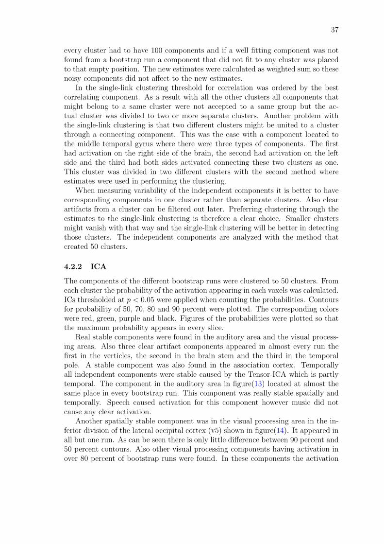
37

every cluster had to have 100 components and if a well fitting component was notfound from a bootstrap run a component that did not fit to any cluster was placedto that empty position. The new estimates were calculated as weighted sum so thesenoisy components did not affect to the new estimates.

In the single-link clustering threshold for correlation was ordered by the bestcorrelating component. As a result with all the other clusters all components thatmight belong to a same cluster were not accepted to a same group but the ac-tual cluster was divided to two or more separate clusters. Another problem withthe single-link clustering is that two different clusters might be united to a clusterthrough a connecting component. This was the case with a component located tothe middle temporal gyrus where there were three types of components. The firsthad activation on the right side of the brain, the second had activation on the leftside and the third had both sides activated connecting these two clusters as one.This cluster was divided in two different clusters with the second method whereestimates were used in performing the clustering.

When measuring variability of the independent components it is better to havecorresponding components in one cluster rather than separate clusters. Also clearartifacts from a cluster can be filtered out later. Preferring clustering through theestimates to the single-link clustering is therefore a clear choice. Smaller clustersmight vanish with that way and the single-link clustering will be better in detectingthose clusters. The independent components are analyzed with the method thatcreated 50 clusters.

4.2.2 ICA

The components of the different bootstrap runs were clustered to 50 clusters. Fromeach cluster the probability of the activation appearing in each voxels was calculated.ICs thresholded at p < 0.05 were applied when counting the probabilities. Contoursfor probability of 50, 70, 80 and 90 percent were plotted. The corresponding colorswere red, green, purple and black. Figures of the probabilities were plotted so thatthe maximum probability appears in every slice.

Real stable components were found in the auditory area and the visual process-ing areas. Also three clear artifact components appeared in almost every run thefirst in the verticles, the second in the brain stem and the third in the temporalpole. A stable component was also found in the association cortex. Temporallyall independent components were stable caused by the Tensor-ICA which is partlytemporal. The component in the auditory area in figure(13) located at almost thesame place in every bootstrap run. This component was really stable spatially andtemporally. Speech caused activation for this component however music did notcause any clear activation.

Another spatially stable component was in the visual processing area in the in-ferior division of the lateral occipital cortex (v5) shown in figure(14). It appeared inall but one run. As can be seen there is only little difference between 90 percent and50 percent contours. Also other visual processing components having activation inover 80 percent of bootstrap runs were found. In these components the activation

38

Figure 13: The contours of the auditory independent component that is activatedduring speech.

39

is wider spread and some runs did not contain these components at all. Compo-nents in the superior division of the lateral occipital cortex, the occipital pole, thesupracalcarine and the cuneal cortex, the precuneous cortex and the lingual gyrusare shown in figures 15, 16, 17, 18 and 19.

Figure 14: The visual proseccing component appearing near the visual prosessingarea V5

Figure 15: The independent component appearing in the superior division of thelateral occipital cortex

The independent component in figure(20) located in the superior parietal lob-ule appeared in 80 runs. Hand movements in the movie seemed to cause most ofthis component’s activation peaks. Activation waged to the right side but in somecomponents there was more activation in the left side. Both sides contained smallerareas of activation in the precentral gyrus in some runs forming a network from ac-tivations. The other component forming a network is found in the superior divisionof the lateral occipital cortex and the middle frontal gyrus figure(21). The thirdnetwork is located in regions of the middle temporal gyrus, the precuneous cortexand the precentral gyrus shown in figure(22).

Near the auditory area in the middle temporal gyrus is a component which isprobably related to language processing. This is a stable component as can be seenfrom figure(23) where the activation appears over 90 percent of the time in the samespatial location.

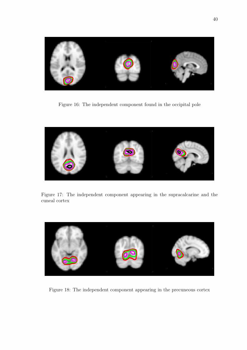
40

Figure 16: The independent component found in the occipital pole

Figure 17: The independent component appearing in the supracalcarine and thecuneal cortex

Figure 18: The independent component appearing in the precuneous cortex

41

Figure 19: The independent component located in the lingual gyrus

Figure 20: The independet component found in in the superior parietal lobule

Figure 21: The independent component containing a network

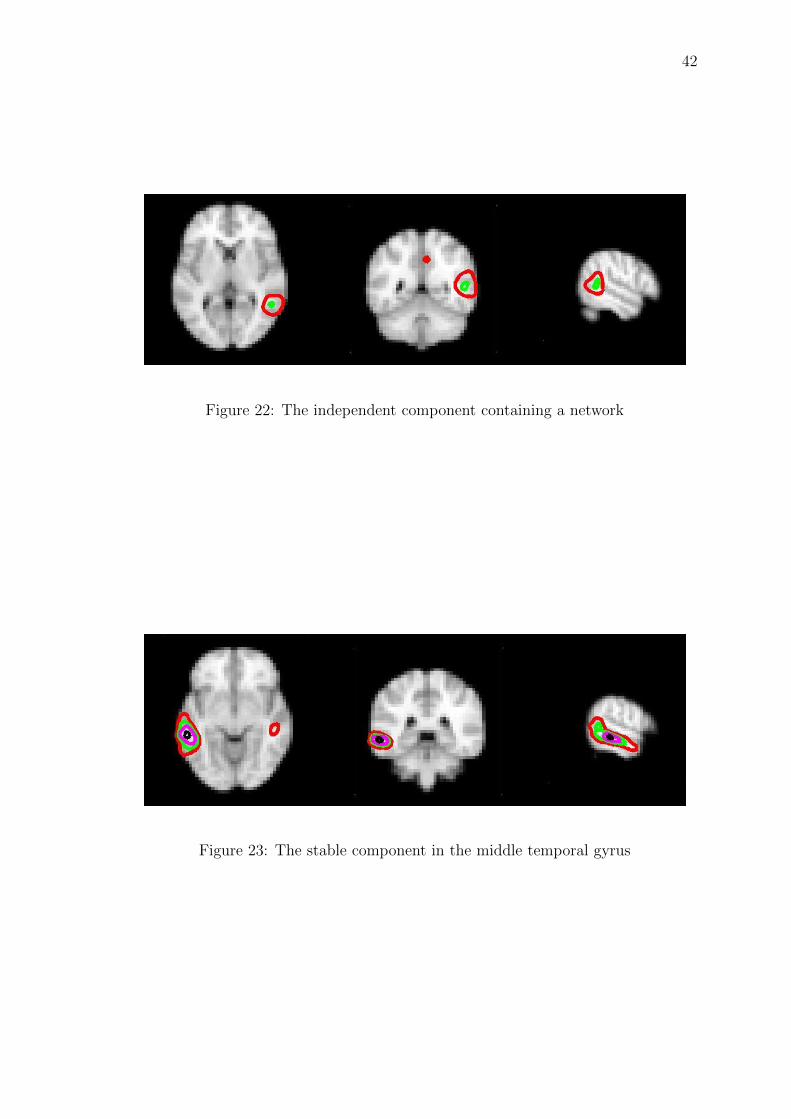
42

Figure 22: The independent component containing a network

Figure 23: The stable component in the middle temporal gyrus

43

4.2.3 Temporal variability

Time series of the components in each cluster were plotted the same way as infigure(24). The times series is from the component shown in figure(22). The redline is the mean of all time series. The different tones of blue represent areas where50, 75 and 100 percents of the time series are located. Many subjects react to astimulus if the mean shows activation. When there is only activation in the quartilebut the mean stays still this means that some subjects react to a stimulus in themovie but the rest do not.

Figure 24: The time series represent areas where 50, 75 and 100 percents of the timeseries are located as different colors. The red line shows the mean.

Components found by the Tensor-ICA were temporally stable as the spreadaround the mean was large only in few time series in the cluster. The most stable wasthe auditory component where the time series of the bootstrap runs looked almostthe same. The other components showed a little bit more variability. The temporal

44

consistency could be expected because Tensor-ICA is not completely spatial but ispartly temporal.

4.3 Comparison of ICA and ISC

In ICA the point of activation can be seen more accurately than in ISC. As ISC iscounted from several time points the activation of IC can be counted for every timepoint separately. From time series of IC many small changes in brain can be seen asISC reacts to more explicit changes. This can be seen in figure(25) where time seriesof the independent component in the parietal area and the number of the same area’ssignificant voxels from the intersubject correlation analysis are presented. There aremore peaks in the IC time series represented in blue which are caused by somestimuli in the movie. These same stimuli are hard to find from the ISC time seriesand some do not appear at all.

When studying people watching a movie ISC finds the scenes that cause similarchanges in every subject’s brain region. With ICA it’s possible to study moreaccurately events inside these scenes. ICA can also separate artifacts from thereal signal and be used as a preprocessing stage for ISC analysis.

45

Figure 25: Time series of the independent component from the parietal area plottedin blue and the number significant voxels in the superior parietal lobule plotted ingreen.

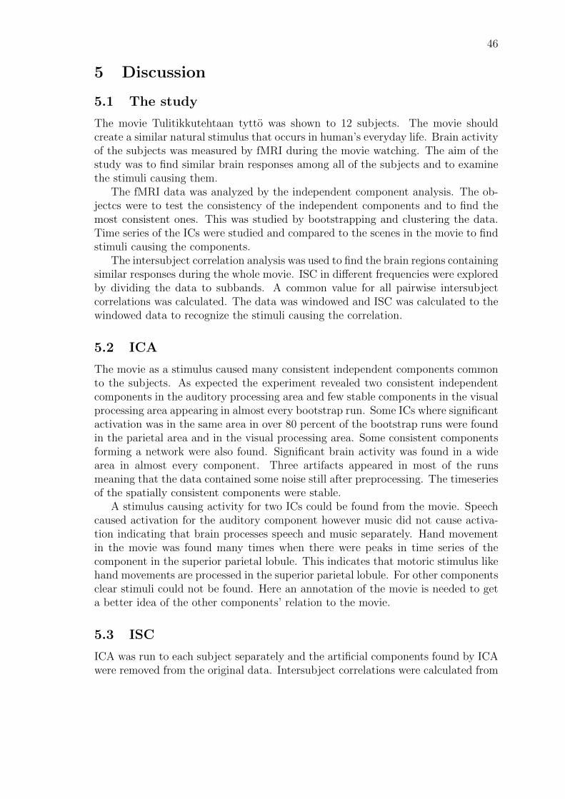
46

5 Discussion

5.1 The study

The movie Tulitikkutehtaan tytto was shown to 12 subjects. The movie shouldcreate a similar natural stimulus that occurs in human’s everyday life. Brain activityof the subjects was measured by fMRI during the movie watching. The aim of thestudy was to find similar brain responses among all of the subjects and to examinethe stimuli causing them.

The fMRI data was analyzed by the independent component analysis. The ob-jectcs were to test the consistency of the independent components and to find themost consistent ones. This was studied by bootstrapping and clustering the data.Time series of the ICs were studied and compared to the scenes in the movie to findstimuli causing the components.

The intersubject correlation analysis was used to find the brain regions containingsimilar responses during the whole movie. ISC in different frequencies were exploredby dividing the data to subbands. A common value for all pairwise intersubjectcorrelations was calculated. The data was windowed and ISC was calculated to thewindowed data to recognize the stimuli causing the correlation.

5.2 ICA

The movie as a stimulus caused many consistent independent components commonto the subjects. As expected the experiment revealed two consistent independentcomponents in the auditory processing area and few stable components in the visualprocessing area appearing in almost every bootstrap run. Some ICs where significantactivation was in the same area in over 80 percent of the bootstrap runs were foundin the parietal area and in the visual processing area. Some consistent componentsforming a network were also found. Significant brain activity was found in a widearea in almost every component. Three artifacts appeared in most of the runsmeaning that the data contained some noise still after preprocessing. The timeseriesof the spatially consistent components were stable.

A stimulus causing activity for two ICs could be found from the movie. Speechcaused activation for the auditory component however music did not cause activa-tion indicating that brain processes speech and music separately. Hand movementin the movie was found many times when there were peaks in time series of thecomponent in the superior parietal lobule. This indicates that motoric stimulus likehand movements are processed in the superior parietal lobule. For other componentsclear stimuli could not be found. Here an annotation of the movie is needed to geta better idea of the other components’ relation to the movie.

5.3 ISC

ICA was run to each subject separately and the artificial components found by ICAwere removed from the original data. Intersubject correlations were calculated from

47

resulting data in fullband and in five subbands. In fullband significant correlationwas found in the auditory and the visual processing areas as expected. There wasalso synchronization in the parietal areas.

The deviation of the data to five subbands revealed the dominance of the audi-tory and the visual processing areas in higher frequencies. These regions and theparietal areas showed synchronization in all subbands. In low frequencies significantcorrelation was also found in frontal parts of the brain.

The intersubject correlation was calculated to the windowed data in fullband.There were scenes in the movie where significant correlation could be found in manybrain regions. During some scenes correlation could only be found in a few regions.There were also scenes where correlation could not be found in any part of the brain.Speech seemed to cause correlation in the auditory processing areas. Voxels in thesuperior parietal lobule correlated when stimuli related to working with hands arepresented. Clear stimuli causing correlation in the other regions could not be found.

5.4 Future research

When ICs and ISCs are studied a good annotation of the movie is needed to geta better idea of the possible stimuli causing the brain responses. With ICA manyartifacts can be found and removed from the data making future studies better. Anautomatic program to remove these artifacts would be rational to use. ISC can becalculated from the windowed data in different frequency bands. The window sizemust be designed so that they are reasonable for the frequencies. More movies haveto be studied to confirm the findings from the study of Tulitikkutehtaan tytto. Newmovies could be designed for the purpose of brain study. The findings from thisstudy could be used in designing the forthcoming movies.

48

References

[1] U. Hasson, Y. Nir, I. Levy, G. Fuhrmann, and R. Malach. Intersubject syn-chronization of cortical activity during natural vision. Science, 303(5664):1634,2004.

[2] A. Bartels and S. Zeki. The chronoarchitecture of the human brainnaturalviewing conditions reveal a time-based anatomy of the brain. NeuroImage,22(1):419–433, 2004.

[3] I.P. Jaaskelainen, K. Koskentalo, M.H. Balk, T. Autti, J. Kauramaki, C. Pom-ren, and M. Sams. Inter-subject synchronization of prefrontal cortex hemody-namic activity during natural viewing. The Open Neuroimaging Journal, 2:14,2008.

[4] D.W. McRobbie, E.A. Moore, M.J. Graves, and M.R. Prince. MRI from Pictureto Proton. Cambridge Univ Pr, 2003.

[5] Aaron Filler. File:spin echo diagram.jpg. http://en.wikipedia.org/wiki/

File:Spin_Echo_Diagram.jpg, July 2009.

[6] S.A. Huettel, A.W. Song, and G. McCarthy. Functional magnetic resonanceimaging. Sinauer Associates Sunderland, MA, 2004.

[7] P. Jezzard, P.M. Matthews, and S.M. Smith. Functional MRI: an introductionto methods. Oxford University Press Oxford, 2001.

[8] M. Jenkinson, P. Bannister, M. Brady, and S. Smith. Improved optimizationfor the robust and accurate linear registration and motion correction of brainimages. Neuroimage, 17(2):825–841, 2002.

[9] Kaveh Vahedipour. Juelich extensible mri simulator. http://www.jemris.

org/jemris/doc/html/ug_JEMRIS_seq.html, September 2008.

[10] S. Clare. Functional MRI: methods and applications. Online document], 9 Aug.2000, 2002.

[11] S.M. Smith. Fast robust automated brain extraction. Human Brain Mapping,17(3):143–155, 2002.

[12] K.H. Hohne and W.A. Hanson. Interactive 3D segmentation of MRI and CTvolumes using morphological operations. Journal of Computer Assisted Tomog-raphy, 16(2):285, 1992.

[13] B. Biswal, E.A. Deyoe, J.S. Hyde, et al. Reduction of physiological fluctuationsin fMRI using digital filters. Magnetic Resonance in Medicine, 35(1):107–113,1996.

[14] C.G. Thomas, R.A. Harshman, and R.S. Menon. Noise reduction in BOLD-based fMRI using component analysis. Neuroimage, 17(3):1521–1537, 2002.

49

[15] T. Kochiyama, T. Morita, T. Okada, Y. Yonekura, M. Matsumura, andN. Sadato. Removing the effects of task-related motion using independent-component analysis. Neuroimage, 25(3):802–814, 2005.

[16] V. Perlbarg, P. Bellec, J.L. Anton, M. Pelegrini-Issac, J. Doyon, and H. Benali.CORSICA: correction of structured noise in fMRI by automatic identificationof ICA components. Magnetic resonance imaging, 25(1):35–46, 2007.

[17] J. Tohka, K. Foerde, A.R. Aron, S.M. Tom, A.W. Toga, and R.A. Poldrack.Automatic independent component labeling for artifact removal in fMRI. Neu-roimage, 39(3):1227–1245, 2008.

[18] A. Hyvarinen and E. Oja. Independent component analysis: algorithms andapplications. Neural networks, 13(4-5):411–430, 2000.

[19] A.J. Bell and T.J. Sejnowski. An information-maximization approach to blindseparation and blind deconvolution. Neural computation, 7(6):1129–1159, 1995.

[20] C.F. Beckmann and S.M. Smith. Probabilistic independent component analy-sis for functional magnetic resonance imaging. IEEE transactions on medicalimaging, 23(2):137–152, 2004.

[21] M.E. Tipping and C.M. Bishop. Mixtures of probabilistic principal componentanalyzers. Neural computation, 11(2):443–482, 1999.

[22] A. Hyvarinen. New approximations of differential entropy for independent com-ponent analysis and projection pursuit. Advances in neural information pro-cessing systems, pages 273–279, 1998.

[23] CM Bishop. Neural networks for pattern recognition. Clarendon, 1995.

[24] A.P. Dempster, N.M. Laird, D.B. Rubin, et al. Maximum likelihood fromincomplete data via the EM algorithm. Journal of the Royal Statistical Society.Series B (Methodological), 39(1):1–38, 1977.

[25] B.S. Everitt and E.T. Bullmore. Mixture model mapping of brain activationin functional magnetic resonance images. Human Brain Mapping, 7(1):1–14,1999.

[26] R.A. Harshman and M.E. Lundy. The PARAFAC model for three-way factoranalysis and multidimensional scaling. Research methods for multimode dataanalysis, pages 122–215, 1984.

[27] CF Beckmann and SM Smith. Tensorial extensions of independent componentanalysis for multisubject FMRI analysis. Neuroimage, 25(1):294–311, 2005.

[28] J-P Kauppi, I Jaaskelainen, M Sams, and J Tohka. Inter-subject correlation ofbrain hemodynamic responses during watching a movie: localization in spaceand frequency. Frontiers in Neuroinformatics.

50

[29] Y. Golland, S. Bentin, H. Gelbard, Y. Benjamini, R. Heller, Y. Nir, U. Hasson,and R. Malach. Extrinsic and intrinsic systems in the posterior cortex of thehuman brain revealed during natural sensory stimulation. Cerebral Cortex,17(4):766, 2007.

[30] S.M. Wilson, I. Molnar-Szakacs, and M. Iacoboni. Beyond superior temporalcortex: intersubject correlations in narrative speech comprehension. CerebralCortex, 18(1):230, 2008.

[31] T. Nichols and S. Hayasaka. Controlling the familywise error rate in functionalneuroimaging: a comparative review. Statistical methods in medical research,12(5):419, 2003.

[32] Y. Benjamini and Y. Hochberg. Controlling the false discovery rate: a practicaland powerful approach to multiple testing. Journal of the Royal StatisticalSociety. Series B (Methodological), pages 289–300, 1995.

[33] Y. Hochberg and A.C. Tamhane. Multiple comparison procedures. Wiley NewYork, 1987.

[34] Y. Benjamini and D. Yekutieli. The control of the false discovery rate in multipletesting under dependency. The Annals of Statistics, 29(4):1165–1188, 2001.

[35] M.J. McKeown, S. Makeig, G.G. Brown, T.P. Jung, S.S. Kindermann, A.J. Bell,and T.J. Sejnowski. Analysis of fMRI data by blind separation into independentspatial components. Human Brain Mapping, 6(3):160–188, 1998.

[36] J. Ylipaavalniemi. Variability of Independent Components in functional Mag-netic Resonance Imaging. PhD thesis, HELSINKI UNIVERSITY OF TECH-NOLOGY, 2005.

[37] Oxford UK Analysis Group, FMRIB. Fmrib software library. http://www.

fmrib.ox.ac.uk/fsl/, January 2010.

[38] J. Tohka, E. Krestyannikov, I.D. Dinov, AM Graham, D.W. Shattuck, U. Ruot-salainen, and A.W. Toga. Genetic algorithms for finite mixture model basedvoxel classification in neuroimaging. IEEE Transactions on Medical Imaging,26(5):696–711, 2007.

[39] D.W. Shattuck, S.R. Sandor-Leahy, K.A. Schaper, D.A. Rottenberg, and R.M.Leahy. Magnetic resonance image tissue classification using a partial volumemodel. NeuroImage, 13(5):856–876, 2001.