boston university dissertationphysics.bu.edu/~bgregor/thesis.pdf · · 2004-06-03boston...
TRANSCRIPT

BOSTON UNIVERSITY
GRADUATE SCHOOL OF ARTS AND SCIENCES
Dissertation
TOTAL INTERNAL REFLECTION AND DYNAMIC LIGHT
SCATTERING MICROSCOPY OF GELS
by
BRIAN F. GREGOR
B.S., Northeastern University, 1998
Submitted in partial fulfillment of the
requirements for the degree of
Doctor of Philosophy
2004
Approved by
First ReaderShyamsunder Erramilli, Ph.D.Professor of Physics
Second ReaderRama Bansil, Ph.D.Professor of Physics

ACKNOWLEDGEMENTS
I wish to thank my advisor, Professor Shyamsunder Erramilli for his guidance,
patience, and instruction over the past several years. It has been a pleasure to work
in his laboratory.
I would like to express my sincere thanks to a number of people who have worked
with me over the course of working on the research for this thesis. In particular,
I would like to thank my first advisor, Professor Bruce Boghosian, and the second
reader on my thesis, Professor Rama Bansil, for their time and assistance. Other
people include Professor Claudio Rebbi, Professor Peter So, Dr. Mi Hong, Dr.
Volkmar Heinreich, Professor Bennett Goldberg, and Professor Anna Swan. I would
also like to thank my fellow graduate students Zhenning Hong, Jonathan Celli,
Huifen Nie, Bradley Turner, Ariel Michaelman, and Euiheon Chung. The physics
office staff, in particular Larry Cicatelli and Mirtha Cabello, were very helpful over
the years as well. The work in this thesis also could not have been completed without
the assistance of the staff of the Boston University machine shop.
On a personal note, I would like to thank my family and friends, especially my
wife Karen, for their encouragement. Without their support the completion of this
thesis would not have been possible.

TOTAL INTERNAL REFLECTION AND DYNAMIC LIGHT
SCATTERING MICROSCOPY OF GELS
(Order No. )
BRIAN F. GREGOR
Boston University Graduate School of Arts and Sciences, 2004
Major Professor: Shyamsunder Erramilli, Professor of Physics
ABSTRACT
Two different techniques which apply optical microscopy in novel ways to the
study of biological systems and materials were built and applied to several samples.
The first is a system for adapting the well-known technique of dynamic light scat-
tering (DLS) to an optical microscope. This instrument can detect and scatter light
from very small volumes, as compared to standard DLS which studies light scat-
tering from volumes 1000x larger. The small scattering volume also allows for the
observation of nonergodic dynamics in appropriate samples. Porcine gastric mucin
(PGM) forms a gel at low pH which lines the epithelial cell layer and acts as a protec-
tive barrier against the acidic stomach environment. The dynamics and microscopic
viscosity of PGM at different pH levels is studied using polystyrene microspheres
as tracer particles. The microscopic viscosity and microrheological properties of
the commercial basement membrane Matrigel are also studied with this instrument.
Matrigel is frequently used to culture cells and its properties remain poorly deter-
mined. Well-characterized and purely synthetic Matrigel substitutes will need to
have the correct rheological and morphological characteristics.
iv

The second instrument designed and built is a microscope which uses an in-
terferometry technique to achieve an improvement in resolution 2.5x better in one
dimension than the Abbe diffraction limit. The technique is based upon the inter-
ference of the evanescent field generated on the surface of a prism by a laser in a
total internal reflection geometry. The enhanced resolution is demonstrated with
fluorescent samples. Additionally, Raman imaging microscopy is demonstrated us-
ing the evanescent field in resonant and non-resonant samples, although attempts at
applying the enhanced resolution technique to the Raman images were ultimately
unsuccessful. Applications of this instrument include high resolution imaging of cell
membranes and macroscopic structures in gels and proteins.
Finally, a third section incorporating previous research on simulations of com-
plex fluids is included. Two dimensional simulations of oil, water, and surfactant
mixtures were computed with a lattice gas method. The simulated systems were
randomly mixed and then the temperature was quenched to a predetermined point.
Spontaneous micellization is observed for a narrow range of temperature quenches,
and the overall growth rate of macroscopic structure is found to follow a Vogel-
Fulcher growth law.
v

Contents
1 Introduction 1
1.1 Prospectus . . . . . . . . . . . . . . . . . . . . . . . . . . . . . . . . . 1
1.2 The Dynamic Light Scattering Microscope . . . . . . . . . . . . . . . 1
1.3 The Standing Wave Total Internal Reflection Microscopy . . . . . . . 4
1.4 Lattice-gas Simulations of Surfactant Systems . . . . . . . . . . . . . 5
1.5 Thesis Organization . . . . . . . . . . . . . . . . . . . . . . . . . . . . 6
1.6 Main Results . . . . . . . . . . . . . . . . . . . . . . . . . . . . . . . 7
2 Optical Microscopy 8
2.1 Diffraction Theory . . . . . . . . . . . . . . . . . . . . . . . . . . . . 8
2.1.1 Fraunhofer Diffraction . . . . . . . . . . . . . . . . . . . . . . 8
2.1.2 Fraunhofer Diffraction of a Circular Aperture . . . . . . . . . 12
2.2 Image Formation . . . . . . . . . . . . . . . . . . . . . . . . . . . . . 14
2.2.1 The Limits of Image Resolution . . . . . . . . . . . . . . . . . 17
2.3 Conclusion . . . . . . . . . . . . . . . . . . . . . . . . . . . . . . . . . 20
3 Light Scattering 22
3.1 Elastic and Inelastic Light Scattering . . . . . . . . . . . . . . . . . . 22
3.2 Elastic Light Scattering . . . . . . . . . . . . . . . . . . . . . . . . . 25
vi

3.2.1 Scattered Intensity . . . . . . . . . . . . . . . . . . . . . . . . 27
3.3 Dynamic Light Scattering . . . . . . . . . . . . . . . . . . . . . . . . 28
3.3.1 Coherence Areas . . . . . . . . . . . . . . . . . . . . . . . . . 30
3.4 Analysis of Light Scattering Data . . . . . . . . . . . . . . . . . . . . 31
3.4.1 Gel Scattering . . . . . . . . . . . . . . . . . . . . . . . . . . . 34
4 Dynamic Light Scattering Experiments 40
4.1 Instrument Details . . . . . . . . . . . . . . . . . . . . . . . . . . . . 40
4.1.1 Calibration and Experiment Setup . . . . . . . . . . . . . . . 43
4.2 Tracer Particle Dynamics . . . . . . . . . . . . . . . . . . . . . . . . . 45
4.3 Surfactants . . . . . . . . . . . . . . . . . . . . . . . . . . . . . . . . 49
4.4 The Mucin Protein . . . . . . . . . . . . . . . . . . . . . . . . . . . . 50
4.5 Mucin Protein Dynamics . . . . . . . . . . . . . . . . . . . . . . . . . 52
4.6 Matrigel . . . . . . . . . . . . . . . . . . . . . . . . . . . . . . . . . . 62
4.7 Matrigel Dynamics . . . . . . . . . . . . . . . . . . . . . . . . . . . . 64
4.7.1 Pure Matrigel . . . . . . . . . . . . . . . . . . . . . . . . . . . 66
4.7.2 109 nm beads in Matrigel . . . . . . . . . . . . . . . . . . . . 67
4.8 Conclusions . . . . . . . . . . . . . . . . . . . . . . . . . . . . . . . . 72
5 Raman Scattering 75
5.1 A Brief History of the Raman Effect . . . . . . . . . . . . . . . . . . 75
5.2 Classical Raman Scattering Theory . . . . . . . . . . . . . . . . . . . 76
5.3 Quantum Mechanical Theory of Raman Scattering . . . . . . . . . . . 80
5.3.1 Polarizability . . . . . . . . . . . . . . . . . . . . . . . . . . . 83
5.3.2 Resonance Raman Scattering . . . . . . . . . . . . . . . . . . 85
5.4 Applications . . . . . . . . . . . . . . . . . . . . . . . . . . . . . . . . 86
vii

6 Total Internal Reflection Microscopy Experiments 89
6.1 Imaging Past the Diffraction Limit . . . . . . . . . . . . . . . . . . . 89
6.2 Total Internal Reflection . . . . . . . . . . . . . . . . . . . . . . . . . 90
6.2.1 The Evanescent Field . . . . . . . . . . . . . . . . . . . . . . . 91
6.3 Standing Wave Total Internal Reflection Microscopy . . . . . . . . . . 94
6.3.1 SWTIRM Simulations . . . . . . . . . . . . . . . . . . . . . . 101
6.4 Deconvolution . . . . . . . . . . . . . . . . . . . . . . . . . . . . . . . 106
6.5 Instrument details . . . . . . . . . . . . . . . . . . . . . . . . . . . . . 107
6.6 Fluorescent Images . . . . . . . . . . . . . . . . . . . . . . . . . . . . 112
6.7 Raman Images . . . . . . . . . . . . . . . . . . . . . . . . . . . . . . 115
6.8 Conclusions . . . . . . . . . . . . . . . . . . . . . . . . . . . . . . . . 125
7 Lattice Gas Simulations of Surfactant Systems 126
7.1 Introduction . . . . . . . . . . . . . . . . . . . . . . . . . . . . . . . . 126
7.2 Background and the Lattice-Gas Automata Model . . . . . . . . . . . 127
7.3 Experiment Details . . . . . . . . . . . . . . . . . . . . . . . . . . . . 131
7.4 Analysis . . . . . . . . . . . . . . . . . . . . . . . . . . . . . . . . . . 132
7.5 Conclusions . . . . . . . . . . . . . . . . . . . . . . . . . . . . . . . . 137
8 Discussions and Conclusions 138
8.1 The Dynamic Light Scattering Microscope . . . . . . . . . . . . . . . 138
8.1.1 Porcine Gastric Mucin . . . . . . . . . . . . . . . . . . . . . . 138
8.1.2 Matrigel . . . . . . . . . . . . . . . . . . . . . . . . . . . . . . 139
8.2 The Standing Wave Total Internal Reflection Microscope . . . . . . . 140
8.3 Lattice Gas Simulations of Surfactant Systems . . . . . . . . . . . . . 140
8.4 Future Work . . . . . . . . . . . . . . . . . . . . . . . . . . . . . . . . 141
viii

A The Stokes-Einstein Relation 142
B Diffusing Wave Spectroscopy 145
Bibliography 146
Curriculum Vitae 158
ix
List of Figures
2.1 Huygen’s Principle . . . . . . . . . . . . . . . . . . . . . . . . . . . . 9
2.2 Derivation of the Helmholtz-Kirchoff equation. . . . . . . . . . . . . . 10
2.3 Point source illumination of the aperture A . . . . . . . . . . . . . . . 12
2.4 Plot of y =[
2J1(x)x
]2
where y = (UU∗)/(π2R4) and x = kζR. . . . . . 14
2.5 Ray diagram for imaging . . . . . . . . . . . . . . . . . . . . . . . . . 15
2.6 Path of light through an optical microscope showing conjugate planes. 17
3.1 Mie scattering of 635.2 nm light by 6 µm beads . . . . . . . . . . . . 23
3.2 Bragg diffraction from lines 10 µm apart on a microscale. . . . . . . . 24
3.3 Light scattered by a molecule . . . . . . . . . . . . . . . . . . . . . . 25
4.1 Block diagram of DLS microscope . . . . . . . . . . . . . . . . . . . . 42
4.2 Photo of DLS microscope . . . . . . . . . . . . . . . . . . . . . . . . 44
4.3 Measured Bragg diffraction peaks . . . . . . . . . . . . . . . . . . . . 46
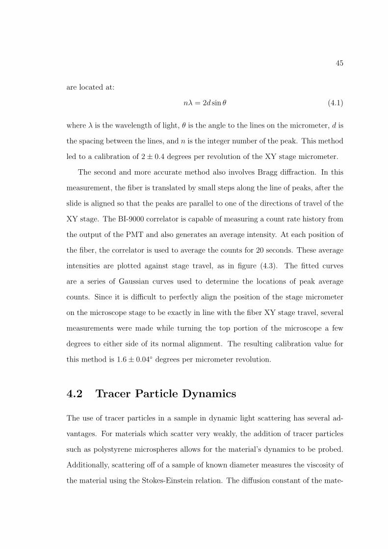
4.4 Diagram of mucin molecule . . . . . . . . . . . . . . . . . . . . . . . 51
4.5 Diagram of macroscopic view of mucin . . . . . . . . . . . . . . . . . 51
4.6 109 nm beads (1% v/v) in 12 mg/ml ph 6 mucin . . . . . . . . . . . . 54
4.7 Applying a stretched exponential to the 109 nm beads in pH 6 mucin 55
4.8 Cage size of ph 6 polymer solution in microscopic cage model . . . . . 57
x

4.9 Power law plus stretched exponential plot of pH 2 mucin . . . . . . . 60
4.10 109 nm beads in pH2 mucin . . . . . . . . . . . . . . . . . . . . . . . 61
4.11 Short-term fit to the structure factor with nonergodic corrections . . 62
4.12 Autocorrelation of 2.03 µm beads . . . . . . . . . . . . . . . . . . . . 65
4.13 Scattering of pure Matrigel . . . . . . . . . . . . . . . . . . . . . . . . 66
4.14 A stretched exponential fit to S(q,τ) for pure Matrigel . . . . . . . . . 67
4.15 g(2)(τ) for 109 nm beads in Matrigel . . . . . . . . . . . . . . . . . . . 68
4.16 A bead trapped in a gel network . . . . . . . . . . . . . . . . . . . . . 70
4.17 Mean square displacement of 510 nm beads in Matrigel . . . . . . . . 71
5.1 C.V. Raman . . . . . . . . . . . . . . . . . . . . . . . . . . . . . . . . 76
5.2 The Morse and harmonic oscillator potentials . . . . . . . . . . . . . 82
5.3 Virtual energy levels . . . . . . . . . . . . . . . . . . . . . . . . . . . 83
5.4 CO2 and its polarizability ellipse . . . . . . . . . . . . . . . . . . . . . 84
5.5 Raman spectrum of polystyrene . . . . . . . . . . . . . . . . . . . . . 87
6.1 Total Internal Reflection . . . . . . . . . . . . . . . . . . . . . . . . . 90
6.2 Electric fields in total internal reflection . . . . . . . . . . . . . . . . 91
6.3 Sketch of SWTIRM setup . . . . . . . . . . . . . . . . . . . . . . . . 101
6.4 27.2 nm/pixel 128× 128 pixels, NA = 1.33, n = 1.51, θ = 47 . . . . . 104
6.5 10 nm/pixel, 128× 128 pixels, NA = 1.33, n = 1.51, θ = 47 . . . . . 105
6.6 Sidebands in the PSF . . . . . . . . . . . . . . . . . . . . . . . . . . . 106
6.7 Deconvolution of a point spread function . . . . . . . . . . . . . . . . 108
6.8 Diagram of SWTIRM microscope . . . . . . . . . . . . . . . . . . . . 109
6.9 CCD calibration image . . . . . . . . . . . . . . . . . . . . . . . . . . 111
6.10 Marconi 47-10 CCD spectral response . . . . . . . . . . . . . . . . . . 111
xi
6.11 The Envy Green fluorophore . . . . . . . . . . . . . . . . . . . . . . . 112
6.12 Normal and SWTIRM images of 60 nm beads. Scale bar is 250 nm. . 114
6.13 Horizontal intensity profiles . . . . . . . . . . . . . . . . . . . . . . . 117
6.14 Chime model of β-carotene. H atoms are yellow, C atoms are cyan . . 117
6.15 White light and Raman images of a chunk of β-carotene . . . . . . . 119
6.16 Raman image of β−carotene . . . . . . . . . . . . . . . . . . . . . . . 120
6.17 Reference Raman spectrum of polystyrene . . . . . . . . . . . . . . . 121
6.18 Raman image of 109 nm polystyrene microspheres. Scale bar is 10 µm123
7.1 The interaction models - (a) color-dipole, (b) dipole-color, and (c)
dipole-dipole . . . . . . . . . . . . . . . . . . . . . . . . . . . . . . . . 129
7.2 β=1.0, 2.0, 3.3 for surfactant concentration=0.225 after 10,000 time
steps . . . . . . . . . . . . . . . . . . . . . . . . . . . . . . . . . . . . 132
7.3 The stretched exponential fit, surfactant concentration 0.245 . . . . . 133
7.4 γ vs. surfactant concentration . . . . . . . . . . . . . . . . . . . . . . 134
7.5 τ vs. temperature . . . . . . . . . . . . . . . . . . . . . . . . . . . . . 134
7.6 1ln(τ)
vs. (T − T∞) . . . . . . . . . . . . . . . . . . . . . . . . . . . . . 135
7.7 Surfactant layer thickness . . . . . . . . . . . . . . . . . . . . . . . . 136
xii

List of Tables
4.1 Summary of 109 nm beads in mucin . . . . . . . . . . . . . . . . . . . 63
4.2 Summary of 109 nm beads in Matrigel . . . . . . . . . . . . . . . . . 68
xiii

List of Abbreviations
CARS Coherent Anti-Stokes RamanCCD Charge Coupled DeviceDPSS Diode Pumped Solid StateDLS Dynamic Light Scattering
FWHM Full Width at Half MaximumHELM Harmonic Excitation Light MicroscopyMCT Mode Coupling TheoryNA Numerical Aperture
NSOM Near-Field Scanning Optical MicroscopyOTF Optical Transfer FunctionPGM Porcine Gastric MucinPSF Point Spread Function
QELS Quasi-Elastic Light ScatteringSERS Surface Enhanced RamanSTED Stimulated Emission Depletion
SWTIRM Standing Wave Total Internal Reflection MicroscopyTIR Total Internal Reflection
xiv

Chapter 1
Introduction
1.1 Prospectus
This thesis presents two different techniques which apply optical microscopy in novel
ways to the study of biological systems and materials. The first is a system for
adapting the well-known technique of dynamic light scattering (DLS) to an optical
microscope. This instrument can detect and scatter light from very small volumes
(1 cubic micron), as compared to standard DLS which studies light scattering from
volumes 1000 × larger. The second is a Raman microscope which uses an inter-
ferometric technique to achieve an improvement in resolution 2.5 × better in one
dimension than the Abbe diffraction limit.
1.2 The Dynamic Light Scattering Microscope
Dynamic light scattering (DLS) is a technique which uses the time varying statistics
of the intensity of the scattered light from a sample to determine a wide variety of
dynamical parameters about the sample. DLS can be used for particle sizing, the

2
study of micellar dynamics, the aggregation behavior of colloids, the dynamics of
phase transitions, and much more. In the typical experimental setup for DLS, a
significant quantity of the scattering sample is required, and in order to enforce the
theoretical assumption that scattered photons are scattered only once the sample
must be quite dilute. Since DLS makes an assumption that scattering dynamics
follow Gaussian statistics, a theoretical minimum of 30 scatterers in the scattering
volume are needed, with a practical minimum of 300 or so. This places limits on
both the concentration and the size of scattering particles.
There have been several previous attempts at adapting the DLS technique to a
microscope stage1 2 which has several advantages. The ability to study very small
quantities of material in the microliter range along with the ability to select the
scattering volume by observation through the microscope optics and translation
of the microscope stage is motivated by several problems. The potential also ex-
ists for performing DLS measurements from the interior volume of individual cells,
although this results in difficult data analysis since there is a wide variety of scatter-
ers in the cell interior. Due to the small scattering volume (10000µm3) involved in
microscope-based DLS nonergodic dynamics can also be observed in gels and glassy
materials. By studying different microscopic regions of the sample, a comparison
the measured scattering intensities between time averages and spatial averages can
be made directly. Secondly, the use of very small volumes means that very expensive
or difficult to obtain samples can be studied. In comparison with standard DLS the
much smaller scattering volume has the effect that the minimum concentration is
higher than in standard DLS in order to meet the minimum number of scatterers.
The previously published designs suffered from several shortcomings1 2. The earlier
instrument from MIT lacked well-defined scattering angles and the design from Prof.
David Weitz’s laboratory at Harvard University suffered from difficulties in calibra-
3
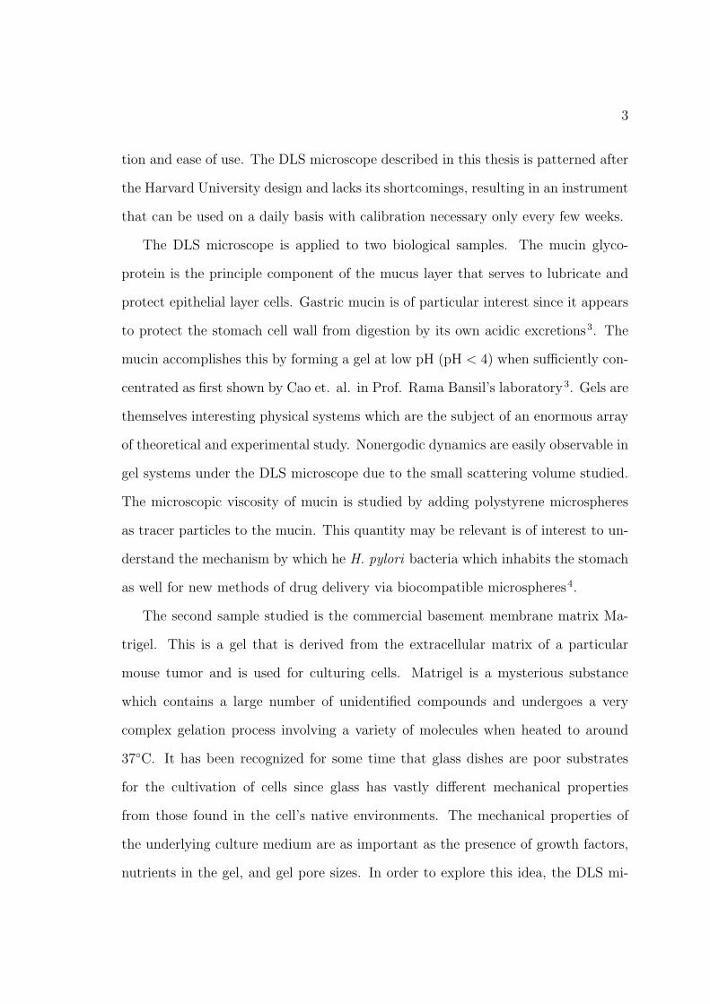
tion and ease of use. The DLS microscope described in this thesis is patterned after
the Harvard University design and lacks its shortcomings, resulting in an instrument
that can be used on a daily basis with calibration necessary only every few weeks.
The DLS microscope is applied to two biological samples. The mucin glyco-
protein is the principle component of the mucus layer that serves to lubricate and
protect epithelial layer cells. Gastric mucin is of particular interest since it appears
to protect the stomach cell wall from digestion by its own acidic excretions3. The
mucin accomplishes this by forming a gel at low pH (pH < 4) when sufficiently con-
centrated as first shown by Cao et. al. in Prof. Rama Bansil’s laboratory3. Gels are
themselves interesting physical systems which are the subject of an enormous array
of theoretical and experimental study. Nonergodic dynamics are easily observable in
gel systems under the DLS microscope due to the small scattering volume studied.
The microscopic viscosity of mucin is studied by adding polystyrene microspheres
as tracer particles to the mucin. This quantity may be relevant is of interest to un-
derstand the mechanism by which he H. pylori bacteria which inhabits the stomach
as well for new methods of drug delivery via biocompatible microspheres4.
The second sample studied is the commercial basement membrane matrix Ma-
trigel. This is a gel that is derived from the extracellular matrix of a particular
mouse tumor and is used for culturing cells. Matrigel is a mysterious substance
which contains a large number of unidentified compounds and undergoes a very
complex gelation process involving a variety of molecules when heated to around
37C. It has been recognized for some time that glass dishes are poor substrates
for the cultivation of cells since glass has vastly different mechanical properties
from those found in the cell’s native environments. The mechanical properties of
the underlying culture medium are as important as the presence of growth factors,
nutrients in the gel, and gel pore sizes. In order to explore this idea, the DLS mi-

4
croscope was applied to study the microrheological properties and microviscosity
of Matrigel using 109 nm and 510 nm diameter polystyrene spheres. Again, the
nonergodic properties of the bead dynamics in the gel are observed. The larger
beads turned out to be quite difficult to study due to their tendency to bind to
the gel network after a period of time and the presence of a wide range of pore
sizes in the gel network. There is a need for purely synthetis and well-characterized
replacements for Matrigel. Understanding the rheological properties of Matrigel is
therefore important. Synthetic substitutes may have to be engineered to match not
only the gel morphology but also the dynamic properties of Matrigel. The elastic
modulus of Matrigel has been determined to be 50.2± 6.0 dynes/cm, a value which
is in the same range as previously published values for polyacrylamide gels5.
1.3 The Standing Wave Total Internal Reflection
Microscopy
A new type of high resolution fluorescence and Raman microscope has been studied
with the goal of extending the resolution of the microscope past the diffraction limit.
There have recently been several methods developed to improve the axial and lateral
resolution of optical microscopy, which is motivated by a wide variety of problems
in biology and solid-state physics. Techniques such as confocal and two-photon
microscopy offer a modest improvement in resolution over standard microscopy,
but emerging techniques offer significantly higher resolution. Methods involving
interferometry include 4π microscopy, I5M 6 microscopy, harmonic excitation light
microscopy (HELM)7, and standing wave total internal reflection microscopy. The
first two improve the axial resolution and the latter two the lateral resolution. Other
techniques such as stimulated emission depletion (STED) microscopy8 9 make use of

5
nonlinear interactions of light with matter to increase the axial or spatial resolution.
Solid immersion lenses (SILs)10 are another technique which increases the resolution
by coupling the near field electric field from the sample with a hemispherical lens.
The standing wave total internal reflection microscope (SWTIRM)11 was in-
vented by Peter So at the Massachusetts Institute of Technology. The microscope
built for this thesis investigates the limits and operational parameters of this mi-
croscope for fluorescence imaging, and attempts to extend the technique to Raman
imaging. Raman imaging microscopy has the advantage over fluorescence of not
needing sample treatment or the introduction of labels for samples to be imaged.
The conclusion of this study is that the power density of the probe laser beam needed
for effective Raman imaging proved difficult to achieve in the total internal reflec-
tion geometry, and the limitations of this technique for Raman microscopy will be
discussed. Techniques with a stronger Raman signal, such as stimulated Raman12,
surface-enhanced Raman13 14, and coherent anti-Stokes Raman15 have the potential
to benefit from this technique, and the prospect for this is discussed.
1.4 Lattice-gas Simulations of Surfactant Systems
In addition to the development of new microscopes, research on computer simula-
tions of oil–water–surfactant systems was performed. A two-dimensional lattice gas
model16 that models oil, water, and surfactant interactions in the same spirit as
electrostatics is used to study the phase separation dynamics of the mixture under
different instantaneous temperature quenches. There does not exist any equivalent
of the Navier-Stokes equations for these types of complex fluids, so the best accessible
theoretical approach to studying the dynamics is in the development of computa-
tional models. The results of the simulations indicate that the size of structures in

6
the fluids grow following a Vogel-Fulcher growth law. Additionally, the simulations
show the growth of stable micelles for certain ranges of temperature quenches.
1.5 Thesis Organization
The thesis is organized as follows. First, in Chapter 2, background material on the
physics of image formation and the operation of microscopes is presented. Chapter 3
introduces the theory of dynamic light scattering and the various methods used to
analyze the data. The design and operation of the DLS microscope is then described,
including information on its merits in comparison with standard DLS experiments.
Chapter 4 contains the results of using the DLS microscope to study the dynamics
of the mucin protein under various conditions.
Chapter 5 introduces the theory of Raman scattering, followed by the theory of
the standing wave-total internal reflection (SWTIRM) technique used to enhance
the resolution of the microscope. The design and operation of the SWTIRM Raman
microscope is then described in detail. Chapter 6 presents the results of imaging
experiements with this instrument on polystyrene beads. Chapter 7 is unrelated
to the rest of the work presented here. This chapter deals with the computational
study of two dimensional oil–water–surfactant dynamics.
Chapter 8 summarizes the results of the thesis and offers guidance for future
related work. The appendices add additional detail to select topics in the thesis.
1.6 Main Results
The design and construction of the DLS microscope resulted in a successful instru-
ment that is fairly straightforward to use and calibrate. Two samples were studied,

7
the porcine gastric mucin protein and the commerical basement membrane Matrigel.
Polystyrene microspheres with a diameter of 109 nm were mixed with the mucin at
pH 6 and pH 2 in order to study the microscopic viscosity and to characterize the
dynamics. The Matrigel was also studied with light scattering from the pure sample
and with the addition of microspheres in order to determine its long time elastic
modulus. The value obtained of 50.2 ± 6.0dynes/cm2 can be considered a target
value for the creation of purely synthetic basement membranes for cell culturing
and artificial organ development.
The development standing wave total internal reflection microscope is a qualified
success. The algorithm and method for enhancing microscope resolution past the
Rayleigh diffraction limit has been demonstrated for fluorescence microscopy with
a resolution of 170 nm in one dimension, a 2.8× improvement. The extension of
this technique to Raman imaging showed that total internal reflection microscopy is
possible, however, image intensity, noise, and elimination of fluorescence background
conspired to prevent a successful high resolution Raman image with the SWTIR
method. Suggestions are included in the relevant chapter to potentially remedy
these problems.
The lattice gas simulations found that a Volgel-Fulcher growth law governs the
growth of structure size after temperature quenches in 2D oil-water-surfactant mix-
tures. Spontaneous micelle growth related to the curvature and thickness of the
surfactant layer was also observed.

Chapter 2
Optical Microscopy
2.1 Diffraction Theory
This chapter serves as an introduction to the theory behind image formation in an
optical microscope, which is central to the behavior of the two optical instruments
described in this thesis. Geometric optics are inadequate for describing the perfor-
mance and resolution capability of imaging systems since the wavelength of light is
not taken into account. Here, Fraunhofer diffraction theory and the Fourier theory
of optics is used to describe the physics of image formation and the resolution limits
of standard optical microscopy.
2.1.1 Fraunhofer Diffraction
The diffraction problem considers a free-space wave incident upon an obstacle or
aperture which locally alters the phase and/or the amplitude of the wave. Huygen’s
principle is used to derive a scattering theory which adequately describes most
diffraction phenomena, as compared with Mie scattering theory which applies only
to the diffraction of a plane wave by conducting and dielectric spheres. Huygen’s

9
Figure 2.1: Huygen’s Principle
principle, as described by Christiaan Huygen in 1690, can be summarized as follows:
“every point on a primary wavefront serves as the source of secondary spherical
wavelets, such that the primary wavefront at some later time is the envelope of
these wavelets. Moreover, the wavelets advance with a speed and frequency equal
to those of the primary wave at each point in space.”17
Figure (2.1) illustrates this idea. The plane wave wavefront on the left can be
considered to be a source of expanding spherical wavefronts as shown on the right
which sum to a plane wave. This is, of course, incorrect since only accelerating
charges emit electromagnetic radiation. The sources of spherical wavefronts also
requires a backwards propagating wave, which is certainly not observed (and is
left out of figure (2.1)). In the end, Huygen’s principle serves as a useful construct
that leads to correct results. Mathematically, Huygen’s principle works by making a
scalar wave approximation in which light is considered to consist of a single complex
scalar variable ψ with angular frequency ω and wave vector k0.
Gustav Kirchoff derived a scalar wave equation with boundary conditions, which
justifies the use of Huygen’s principle. Substituting a time-dependent electromag-

10
Figure 2.2: Derivation of the Helmholtz-Kirchoff equation.
netic wave function U(~r) = exp(−iωt) satisfies the Helmholtz equation (∇2+k2)U =
0 where k = ω/c. Following the derivations in references (18) and (19), we let U ′ be
a trial function that along with U possesses continuous first and second derivatives
along a closed surface S that bounds a volume v as shown in figure (2.2). Green’s
theorem gives:
∫ ∫ ∫
v
(U∇2U ′ − U ′∇2U)dv = −∫ ∫
S
(U
∂U ′
∂n− U ′∂U
∂n
)dS (2.1)
The left hand side of equation (2.1) is 0 using the Helmholtz equation. If we now
make the assumption that U ′ is a spherical scalar wave, U ′(x, y, z) = eiks/s where s
is the distance from point P , a point inside the volume v, to (x, y, z), we have:
∫ ∫
S
+
∫ ∫
S′
[U
∂
∂n
(eiks
s
)− eiks
s
∂U
∂n
]dS = 0 (2.2)
Since there is U ′ blows up at s = 0, P must be excluded from the integration.

11
To resolve this, a small sphere of radius ε with surface S ′ has been constructed to
surround P . This results in:
∫ ∫
S
(U
∂U ′
∂n− U ′∂U
∂n
)dS = −
∫ ∫
S′
[U
eiks
s
(ik − 1
s
)− eiks
s
∂U
∂n
]dS ′
= −∫ ∫
Ω
[U
eikε
ε
(ik − 1
ε
)− eikε
ε
∂U
∂s
]ε2dΩ
where dΩ is an element of the solid angle. The integral over S is independent of ε and
can be replaced by its limiting value as ε → 0. The right hand side has two terms,
ikU exp(iks)/s and −(exp(iks)/s)∂U/∂n which do not contribute, and the middle
term contributes 4πU(P ). The final result is the integral theorem of Helmholtz and
Kirchoff :
U(P ) =1
4π
∫ ∫
S
[U
∂
∂n
(1
s
)− 1
s
∂U
∂n
]dS (2.3)
This is the analytical expression for the wave equation and applies to any solution U
and any surface S enclosing the origin. If illumination by a point source is considered
(figure (2.3)) then the result is the Fresnel-Kirchoff diffraction formula:
U(P ) = −iA
2λ
∫ ∫
A
eik(r+s)
rs[cos(n, r)− cos(n, s)]dS (2.4)
Figure (2.3) shows the wave function U at point P after the aperture A is illumi-
nated with a point source radiating spherical waves. In the paraxial limit where the
radiation and observation points are coaxial, the cosine terms are 1 and −1, respec-
tively. In order to describe Fraunhofer diffraction, let us consider a situation where
radiation strikes a diffracting mask R with transmission f(r). Let the observation
point P be at distance d from the mask and the source at a point with a distance L
along the axis to the observation point. If the incoming wave has wavenumber k0,

12
Figure 2.3: Point source illumination of the aperture A
then the field at P is:
U(P ) = −ik0A
2πeik0L
∫ ∫
R
f(r)
deik0dd2r (2.5)
The observed intensity at P is I = UU∗. The rate of change of the phase k0d with
respect to the diameter d determines the classification into Fresnel or Fraunhofer
diffraction. This depends on three factors: the distance d, the size of the trans-
mitting aperture f(r), and the wavelength. If the rate of change is linear, then it
is Fraunhofer diffraction, and if it contains higher order terms, then the diffraction
is Fresnel diffraction. Fortunately, in microscopy the more important case is the
simpler one of Fraunhofer diffraction.
2.1.2 Fraunhofer Diffraction of a Circular Aperture
The case of diffraction from a circular aperture is relevant for the performance of
a microscope objective lens. The detectors in microscopy (eyeballs, CCD cameras,
film) measure the intensity of diffracted light and so the phase information is lost.

13
Equation (2.5) can be re-written without those terms:
U(u, v) =
∫ ∫f(x, y)e−ik(ux+uy)dxdy (2.6)
The terms u and v are the coordinates for measuring U on an image plane with the
aperture defined by f(x, y) on the sample plane. For a circular aperture of radius R,
using polar coordinates where x = ρ cos θ and y = ρ sin θ, we have for the diffraction
pattern coordinates u ≡ ζ cos φ and v ≡ ζ sin φ. Re-writing equation (2.6) we have:
U(u, v) =
∫ R
0
∫ 2π
0
e−kρζ cos φ cos θ+ρζ sin φ sin θρdρdθ (2.7)
=
∫ R
0
∫ 2π
0
e−ikρζ cos(θ−φ)ρdρdθ (2.8)
The following integral representation of the Bessel function Jn(z) is useful here20:
Jn(z) =i−n
2π
∫ 2π
0
eiz cos αeinαdα (2.9)
Equation (2.8) is then written as:
U(ζ, φ) = 2π
∫ a
0
J0(kζρ)ρdρ (2.10)
The recurrence relation:
d
dx
[xn+1Jn+1(x)
]= xn+1Jn(x) (2.11)
can be applied which gives for n = 0
∫ x
0
x′J0(x′)dx′ = xJ1(x) (2.12)

14
−10 −5 0 5 100
0.2
0.4
0.6
0.8
1
x
y
Figure 2.4: Plot of y =[
2J1(x)x
]2
where y = (UU∗)/(π2R4) and x = kζR.
Combining equations (2.12) and (2.10) gives the final form for U:
U(ζ, φ) = πR2
[2J1(kζR)
kζR
](2.13)
The functional form of the intensity, UU∗, which would be measured by the detector
is plotted in figure (2.4) and shows how light from a point source is spread by a
circular aperture.
2.2 Image Formation
Ernst Abbe proposed a theory of image formation in 1867. His method is straight-
forward and considered the image formed by a lens and light striking a periodic
grating of infinite length. This simple model allows for an estimate of the resolution
of the image. A more formal treatment, which is described here, involves treating
the process of image formation as a pair of Fourier transforms of the illuminated

15
x x’ ξ=uF/k0lens
L
O
B
A P
F I z
Q
θ θ’
U V
Figure 2.5: Ray diagram for imaging
object.
This description of imaging and image resolution is based on the scalar wave
theory described previously and is explicitly described in one dimension only, al-
though the extension to two dimensions is straight forward. Figure (2.5) illustrates
the situation: an object at point O is illuminated, and a complex wave f(x) leaving
the object is focused by the lens to its focal plane, F . U is the distance from the
object to the lens (where the lens is assumed to be infinitely thin), F is the focal
length of the lens, and V is the distance from the lens to the observation point.
Points A and B are points on the lens, and point P is a point on the focal plane of
the lens. Rewriting equation (2.6) in one dimension gives for the amplitude at P ,
with a phase factor from the path OAP :
U(u) = eik0OAP
∫ ∞
−∞f(x)e−iuxdx (2.14)
where k0 = 2πλ
and u = k0 sin θ which corresponds to point P on the focal plane.
Huygen’s principle can be used to calculate the amplitude U ′(x′) at point Q. The

16
optical distance PQ is:
PQ =(PI
2+ x′2 − 2x′PI sin θ′
) 12
(2.15)
= PI − x′ sin θ′ (2.16)
where equation (2.16) is accurate when x′ ¿ PI. The Abbe sine condition which
states that in the imaging of an infinite diffraction grating a point at angle θj is
imaged at angle θ′.sin θj
sin θ′= m (2.17)
Maximum resolution is achieved when the condition in equation (2.17) is satisfied
where m is the magnification of the lens. When this condition is true the largest
possible angles of refracted light are captured by the lens. Applying this condition
to equation (2.16) gives:
PQ = PI − x′umk0
. (2.18)
The amplitude at Q can now be written:
U ′(x′) =
∫ ∞
−∞U(u)eik0PQdu (2.19)
=
∫ ∞
−∞eik0PIU(u)e−ix′u/mdu. (2.20)
Inserting equation (2.14) gives an equation of two Fourier transforms:
U ′(x′) =
∫ ∞
−∞eik0(OAP+PI)
∫ ∞
−∞f(x)e−iuxe−iux′/mdxdu (2.21)
The phase factor exp(ik0(OAP +PI)) is a constant exp(−ik0OI) if the planes F and
I are conjugate. Two planes are conjugate if there is a one-to-one correspondence

17
Figure 2.6: Path of light through an optical microscope showing conjugate planes.
between each point on the two planes. This double Fourier transform then becomes:
U ′(x′) = e−ik0OIf
(−x′
m
)(2.22)
and the final result is that the projected image is inverted and magnified by m. The
conjugate planes in a microscope are illustrated in figure (2.6).
2.2.1 The Limits of Image Resolution
The resolution of a microscope depends upon the highest angle gathered of the light
that is scattered from the object. This can be deduced from the Abbe model of
an infinite periodic object with illumination by coherent light. If the object has a

18
period d, the first order is at angle θ1 given by:
sin θ1 =λ
d. (2.23)
The imaging lens captures light scattered up to the angle α between the lens edge
and the sample. If there is a medium (such as oil or water) between the lens and
the sample with an index of refraction n, the effective wavelength is λn. In order for
the lens to image the object of period d, α must be greater than θ1. Shuffling the
previous equation then gives:
dmin =λ
n sin α=
λ
NA(2.24)
where NA = n sin α. NA is referred to as the numerical aperture of the lens. The
illumination of the object has a significant effect on the image resolution. In the
Fourier expansion of the illuminating light, only the zeroth and first order terms are
needed to resolve this level of detail.
If the illuminating light in figure (2.5) is not only along the z-axis but also at
an angle to the axis, then there are additional contributions to equation (2.24). If
the incident wave-vector has direction cosines (l0,m0, n0) then the phase at a point
x is altered. The new phase is advanced by k0l0x with respect to the phase at O.
Equation (2.14) is written the same but u is redefined as:
u = k0(l − l0). (2.25)
If θx is the angle between the x component of the incoming illuminating wave vector

19
and the z-axis, the l = sin(θx) and
u = k0(sin(θx)− sin(θx0).) (2.26)
Next, it is assumed that a feature of the diffraction pattern appears at an angle of
deviation θx − θx0 with respect to the incoming wave vector. Then u can be set to
a constant, and equation (2.26) can be re-written as:
u = const = 2k0 sin
(θx − θx0
2
)cos
(θx + θx0
2
). (2.27)
The factor (θx − θx0) has its minimum value when θx = −θx0, called the condition
of minimum deviation, which experimentally is the condition when the numerical
aperture of the illuminating condenser lens is equal to that of the numerical aperture
of the microscope objective. If the illuminating light is entering at angle α and the
condition for minimum deviation is met then the factor of 2 from equation (2.27) is
included. The final resolution for the object is therefore:
dmin =λ
2NA(2.28)
In the case on completely incoherent light, the resolution is improved somewhat.
Completely incoherent illumination occurs, for example, when imaging fluorescent
objects or Raman scattered light. The diffraction pattern of a circular aperture is
a Bessel function as described in equation (2.13). The intensity measured from an
aperture of diameter D as a function of angle θ is:
I(θ) =
[2J1(
12k0D sin θ)
12k0D sin θ
]2
. (2.29)

20
The Rayleigh criterion for resolution states that two objects can be resolved when
the central maximum of one lies outside the first minimum of the other. I(θ) has a
minimum at the same point as J1(x) at x = 3.83. Therefore we have:
1
2k0D sin θ =
πD sin θ
λ= 3.83 (2.30)
The quantity sin θ is the NA of the system, and again an index of refraction n of
the intervening medium can be included:
D =3.83λ
πn sin θ=
1.22λ
NA(2.31)
As before when the Abbe resolution was considered an additional factor of 2 is picked
up when the illumination is oblique to the object at angle θ, for a final resolution
of:
D =1.22λ
2NA=
0.61λ
NA(2.32)
The resolution here is slightly worse than for coherent illumination. This is consid-
ered the ideal resolution possible for fluorescence and Raman imaging. The instru-
ment described in Chapter 6 demonstrates one method for imaging well past this
limit.
2.3 Conclusion
This chapter has described the performance of an optical microscope based on
Fourier theory. Fraunhofer diffraction causes finite apertures to spread out the
image of a point source. This effect limits the image resolution since microscope
lenses are of course limited to finite size and therefore to a limit in the angle at
21
which light diffracted by the sample can be collected. The Abbe sine condition was
applied to determine the final resolution of a light microscope using incoherent light.
This resolution limit is a factor in the performance of the light scattering microscope
(Chapter 4) and is addressed directly in the standing wave-total internal reflection
microscope (Chapter 6).

Chapter 3
Light Scattering
3.1 Elastic and Inelastic Light Scattering
The interaction of visible wavelengths of light and matter gives rise to a wide variety
of phenomena. The case in particular that is of interest here is the scattering of
light by matter. For a given incident wave of wavelength λi, the scattered light can
have either the same wavelength or it can be shifted in either direction. Elastically
scattered light has the same wavelength, (λi = λs), and is frequently referred to as
Rayleigh scattered light, in honor of Lord Rayleigh who was the first to explain that
the intensity of scattered light varies as 1/λ4 in the 19th century. If λi 6= λs then
the scattering is referred to as inelastic. Light scattered with a longer wavelength
is referred to as Stokes radiation, and light scattered with a shorter wavelength is
referred to as anti-Stokes radiation.
There are a wide variety of elastic scattering phenomena. What follows is a
brief description of a few that are of interest in this work. Mie scattering occurs
when the scatterer is much larger than the wavelength of the incident light. The
only analytic solution to the Mie scattering problem involves light scattering from
23
2
4
6
30
210
60
240
90
270
120
300
150
330
180 0
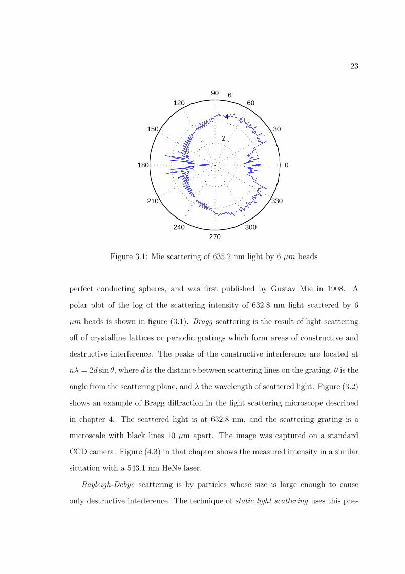
Figure 3.1: Mie scattering of 635.2 nm light by 6 µm beads
perfect conducting spheres, and was first published by Gustav Mie in 1908. A
polar plot of the log of the scattering intensity of 632.8 nm light scattered by 6
µm beads is shown in figure (3.1). Bragg scattering is the result of light scattering
off of crystalline lattices or periodic gratings which form areas of constructive and
destructive interference. The peaks of the constructive interference are located at
nλ = 2d sin θ, where d is the distance between scattering lines on the grating, θ is the
angle from the scattering plane, and λ the wavelength of scattered light. Figure (3.2)
shows an example of Bragg diffraction in the light scattering microscope described
in chapter 4. The scattered light is at 632.8 nm, and the scattering grating is a
microscale with black lines 10 µm apart. The image was captured on a standard
CCD camera. Figure (4.3) in that chapter shows the measured intensity in a similar
situation with a 543.1 nm HeNe laser.
Rayleigh-Debye scattering is by particles whose size is large enough to cause
only destructive interference. The technique of static light scattering uses this phe-

24
Figure 3.2: Bragg diffraction from lines 10 µm apart on a microscale.
nomena to measure time-averaged properties of the scattering material. Here the
interest is in measuring the angle-dependent scattered light intensity which gives the
static structure factor S(q). Techniques that measure the time-varying properties
of singly scattered light are called dynamic light scattering (DLS). Here, the interest
is in measuring the angle-dependent scattered light intensity. In the diffusing wave
spectroscopy technique21, the light is assumed to be multiply scattered and the light
path through the sample is modeled as a diffusion process.
Inelastic light scattering phenomena include Raman scattering. The vibrational
spectrum of a molecule can also be directly measured using infrared absorption
spectroscopy. The Raman effect is the subject of chapter 5, and is described in
detail there.

25
Figure 3.3: Light scattered by a molecule
3.2 Elastic Light Scattering
As mentioned previously, the term “dynamic light scattering” refers to techniques
that measure the time varying statistics of scattered light. Another name for this
technique is quasi-elastic light scattering (QELS). The analytic solution to the in-
tensity of scattered light is derived from Maxwell’s equations. As the light passed
through a dielectric medium, its oscillating electric field induces a dipole moment
in the medium at each point in its path. This can be solved in two ways22, either
by summing the contributions from the induced dipole fields that reach a point x,
or by requiring that the total field E = Ei + Es (where Ei is the incident light and

26
Es the scattered light) satisfies Maxwell’s equations in the presence of matter:
∇ ·D = ρ (3.1)
∇× E = −∂B
∂t(3.2)
∇ ·B = 0 (3.3)
∇×H = J +∂D
∂t(3.4)
The scattered electric field at a point x is then:
Es =1
4πR
(ε0
ε
)~∇×
~∇×
∫
v
∫ ∞
t′=−∞∆χe(x
′, t′)Ei(x′, t′)
×∂
[t′ − t +
1
cm
(R− r′ · R)
]dx′dt′
(3.5)
The quantity v is the scattering volume. The scattering vector q is defined as
q = ki − ks (3.6)
and its magnitude q is
q = |q| = 4πn
λsin (θ/2). (3.7)
As shown in figure (3.3) R is the scattering vector to point x. The electric suscepti-
bility χ is defined as the ratio of the polarization of the sample P to the electric field
E: χ = P/(ε0E). ∆χe is the fluctuating electric susceptibility that is scattering the
light with frequency ω:
∆χe(R, t) = ∆χeei(q·R−ωt). (3.8)

27
The incoming electric field is:
Ei(R, T ) = E0i e
i(ki·R−ωit). (3.9)
If we consider the limit of small small frequency shifts where cm is the speed of
light in the medium we have ks = (ωi/cm) and ω ¿ ωi. The scattered electric field
becomes:
Es(R, t) =1
4πR
(ε0
ε
)~∇R×~∇R×E0
i ei(ks·R−ωit)
×∫
v
∆χe(r′, t)eiq·r′d3r′ (3.10)
The double curl term can be solved using an explicit expansion in terms of spherical
coordinates of the electric dipole field22. The result of this solution is an expression
for the scattered electric field in terms of ∆χe:
Es = ks×(ks×E0i )
(ε0
ε
) ei(ks·R−ωit)
4πR
×∫
v
∆χe(r′, t)eiq·r′dr′ (3.11)
The phase factor exp[iq · r′] is the interference between the wavelets scattered by
the volume elements d3r′, and the factor exp[i(ksR− ωit)] is the wave scattered by
the origin.
3.2.1 Scattered Intensity
The detectors used in the various types of dynamic light scattering a are sensitive to
the intensity of the scattered light, not to the magnitude of the electric field. This is
aTypically, photomultiplier tubes or avalanche photodiodes.

28
equivalent to the time average of the Poynting vector S = E×H that expresses the
energy transferred to the detector23 where H is the magnetic field. The measured
intensity at scattering vector q can be written as:
Is(q, t) = QeRe〈S〉
=Qe
2Re〈Es×H∗
s〉
=Qe
2
√ε
µEs(q, t)E∗
s (q, t) (3.12)
Here, Qe expresses the quantum efficiency of the detector. The intensity can be
further characterized by considering the turbidity of the sample, which is defined as:
τ ∗ =1
dlog
(Ii
It
)(3.13)
where τ ∗ is the turbidity, d is the optical path length in the sample, and It is the
transmitted intensity.
3.3 Dynamic Light Scattering
In DLS experiments, the intensity of scattered light is measured and the output
is analyzed in one of two ways, either by examining the power spectrum of the
signal via a Fourier transform (“quasi-elastic light scattering”) or by calculating the
time correlation function of the signal (“photon correlation spectroscopy”). The
latter method is more popular and is the one used in these experiments. The time
correlation function is defined24 for a signal I(t) as:
G(τ) = 〈I(0)I(τ)〉t = limT→∞
∫ T
−T
I(t)(t + τ)dt (3.14)

29
This function has the advantage over the spectral method due to the relative ease
of its implementation in digital hardware. However, the power spectrum S(ω) and
the correlation function contain the same information and are forward and inverse
Fourier transforms of each other by the Wiener-Khintchine theorem:
G(τ) =
∫ ∞
−∞S(ω)eiωτdω (3.15)
S(ω) =1
2π
∫ ∞
−∞G(τ)e−iωτdτ (3.16)
In DLS measurements the desired correlation function is that of the scattered electric
fields, written as G(1) = 〈Es(0)∗Es(τ)〉t. This is called the first order electric field
autocorrelation function. The second order electric field correlation is the measured
intensity autocorrelation function at the detector, G(2)(τ). The normalized versions
of these functions are:
g(1)(τ) =〈Es(0)∗Es(τ)〉t〈|Es(0)|2〉t (3.17)
g(2)(τ) =〈Is(0)Is(τ)〉t〈|Is(0)|2〉t (3.18)
G(1)(τ) can also be written to make explicit the relation between the measured signal
and fluctuations in the scattering medium:
G(1)(τ) = 〈∆χe(q, 0)∆χe(q, τ)〉t. (3.19)
The time varying intensity of the scattered light is assumed to be from Brownian
motion of the scatteres, which is an assumption that leads to the time variations

30
obeying Gaussian statistics. If this is true, then the two functions g(1) and g(2) are
related by the Siegert relation:
g(2)(τ) = 1 +∣∣g(1)(τ)
∣∣2 (3.20)
Since experimental conditions are not taken into account in equation (3.20), this is
more reasonably stated for actual data with a set of constants (A and B) that are
fit to the data:
G(2)(τ) = B + A|g(1)(τ)|2 (3.21)
The constant B = 〈I〉2 is related to the square of the time averaged scattering
intensity and A = 〈I2〉 − 〈I〉2 is a measure of the dynamic amplitude.
3.3.1 Coherence Areas
In order to measure time correlations it is required that the detector is capable of
making measurements on a time scale smaller than the relaxation times of fluctu-
ations in the sample which lets us study the time correlations. Another important
consideration is the effect of spatial averaging by the detector due to its finite area.
Scattering signals originating from two different points in the sample will be coher-
ent if the fluctuations are correlated, however, if these two points are two far away
they will not be correlated. This problem gives rise to the concept of a coherence
area, which is the relationship between the scattering volume in the sample in which
all of the scattered photons are correlated and the distance to the detector. This
is computed by consideration of the phase integral of equation (3.11). Lastovska22
has shown that for the case of scattering in the xy plane by a parallelpiped with
31
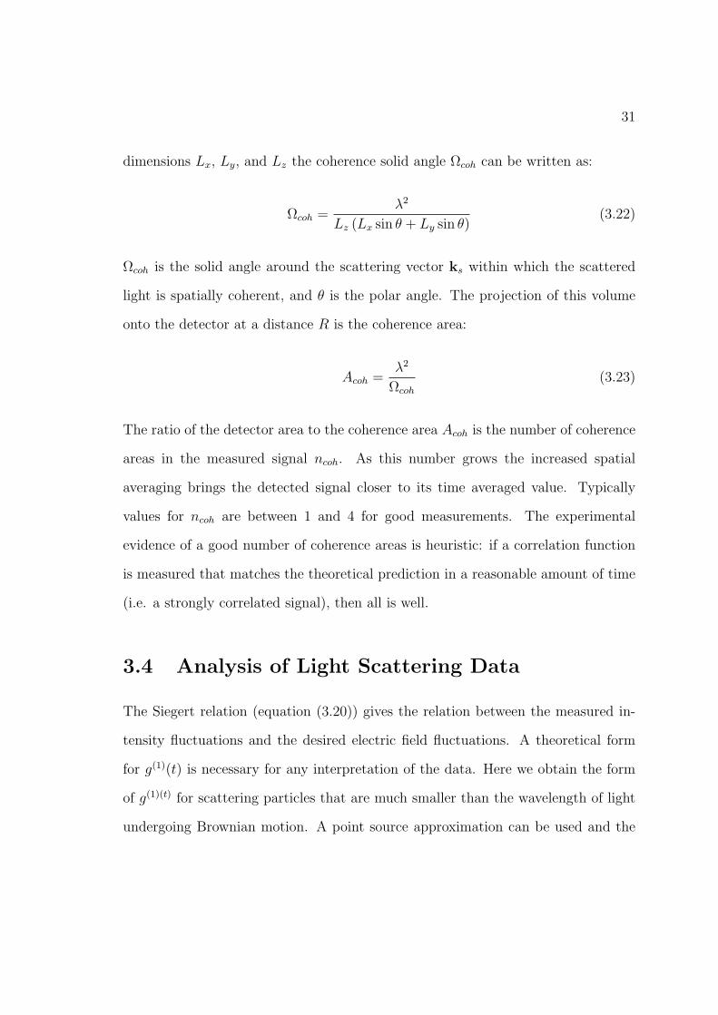
dimensions Lx, Ly, and Lz the coherence solid angle Ωcoh can be written as:
Ωcoh =λ2
Lz (Lx sin θ + Ly sin θ)(3.22)
Ωcoh is the solid angle around the scattering vector ks within which the scattered
light is spatially coherent, and θ is the polar angle. The projection of this volume
onto the detector at a distance R is the coherence area:
Acoh =λ2
Ωcoh
(3.23)
The ratio of the detector area to the coherence area Acoh is the number of coherence
areas in the measured signal ncoh. As this number grows the increased spatial
averaging brings the detected signal closer to its time averaged value. Typically
values for ncoh are between 1 and 4 for good measurements. The experimental
evidence of a good number of coherence areas is heuristic: if a correlation function
is measured that matches the theoretical prediction in a reasonable amount of time
(i.e. a strongly correlated signal), then all is well.
3.4 Analysis of Light Scattering Data
The Siegert relation (equation (3.20)) gives the relation between the measured in-
tensity fluctuations and the desired electric field fluctuations. A theoretical form
for g(1)(t) is necessary for any interpretation of the data. Here we obtain the form
of g(1)(t) for scattering particles that are much smaller than the wavelength of light
undergoing Brownian motion. A point source approximation can be used and the
32
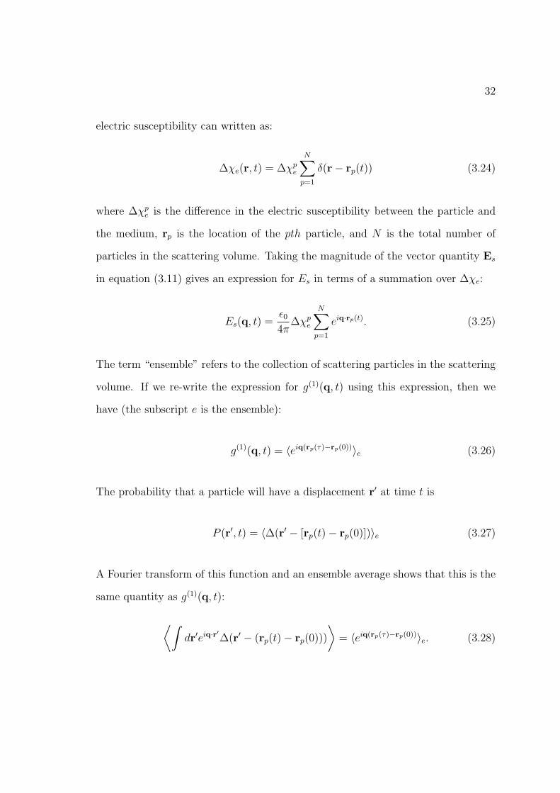
electric susceptibility can written as:
∆χe(r, t) = ∆χpe
N∑p=1
δ(r− rp(t)) (3.24)
where ∆χpe is the difference in the electric susceptibility between the particle and
the medium, rp is the location of the pth particle, and N is the total number of
particles in the scattering volume. Taking the magnitude of the vector quantity Es
in equation (3.11) gives an expression for Es in terms of a summation over ∆χe:
Es(q, t) =ε0
4π∆χp
e
N∑p=1
eiq·rp(t). (3.25)
The term “ensemble” refers to the collection of scattering particles in the scattering
volume. If we re-write the expression for g(1)(q, t) using this expression, then we
have (the subscript e is the ensemble):
g(1)(q, t) = 〈eiq(rp(τ)−rp(0))〉e (3.26)
The probability that a particle will have a displacement r′ at time t is
P (r′, t) = 〈∆(r′ − [rp(t)− rp(0)])〉e (3.27)
A Fourier transform of this function and an ensemble average shows that this is the
same quantity as g(1)(q, t):
⟨∫dr′eiq·r′∆(r′ − (rp(t)− rp(0)))
⟩= 〈eiq(rp(τ)−rp(0))〉e. (3.28)
33
If the particle is assumed to be undergoing a random walk trajectory, then its
dynamics satisfy the diffusion equation:
∂
∂tP (r′, t) + v · ∇P (r′, t) = D∇2P (r′, t) (3.29)
The vector v represents drift velocity in the general case of an external flow. This
equation can be Fourier transformed and g(1)(q, τ) substituted to give an expression
for g(1) in terms of the diffusion equation:
∂
∂tg(1)(q, τ) + iv · qg(1)(q, τ) = D∇2g(1)(q, τ). (3.30)
Once the initial condition g(1)(q, 0) = 1 is applied the solution is straightforward
and yields:
g(1)(q, τ) = e−Dq2τeiq·vτ . (3.31)
The second exponential term is a phase factor that is lost in the intensity measure-
ment, and the measured intensity function is therefore:
G(2)(τ) = A + B|g(1)(q, t)|2 = A + Be−2Dq2τ . (3.32)
The fitting parameters A, B, and D are typically determined by using least-squares
routines. If the scattering particle is assumed to be spherical, the Stokes-Einstein
relation can be used to determine a hydrodynamic radius for the particle or the fluid
viscosity:
D =kT
6πηR(3.33)
where k is Boltzmann’s constant, T is the temperature, η the viscosity, and R
the hydrodynamic (or effective) radius of the particle. This equation is limited to

34
particular situations. If the sample is know to be polydisperse, then this equation
becomes the sum of several exponents, or in the continuum limit becomes:
G(2)(τ) = A +
∫ ∞
0
B(D)e−Dq2τdD (3.34)
The inversion of this equation requires an inverse Laplace transform, which is numer-
ically extremely difficult because this is an underdetermined problem in which there
are many possible solutions to the problem. Various special algorithms have been
used to perform this inverse transform specifically for light scattering data, includ-
ing the well-known CONTIN25 and REPES26 programs. If the scattering particle
is undergoing non-diffusive behavior, for example if it is diffusing in a semidilute
polymer solution where the interacting polymer chains influences the the dynamics,
then equation (3.32) will not be accurate and a different theoretical function will
needed.
3.4.1 Gel Scattering
The autocorrelation function of light scattered by particles trapped in a gel does not
follow the assumption of Gaussian dynamics used in the previous section. In this
case, the particles are not free to move through phase space due to the constraints on
their movement by the gel network. These dynamics are referred to as nonergodic.
Ergodic systems are those in which averages of dynamic quantities over the ensemble
and over time are the same. Additionally, some of the scattering particles will be
completely trapped in the gel (“frozen in”) while others will diffuse about in limited
regions. A model to properly account for nonergodic dynamics for the analysis of
light scattering data was developed by Peter Pusey27 28 in 1989.
The scattered electric field is not described as a zero-mean complex Gaussian
35
variable due to the constrained motion of the scatterers. Mathematically, this means
that the particle movement of particle i at position ri(τ) that is detected at scatter-
ing vector q have a phase factor q · ri(τ) that does not undergo large fluctuations
with respect to 2π in any appreciable length of time. The nonergodicity of the
sample is expressed in a center-of-mass equation for the position of the scattering
particle:
rj(τ) = Rj + ∆j(τ) (3.35)
where ∆j is the movement of the particle about its equilibrium position Rj. These
are further defined as:
Rj = 〈rj(τ)〉t (3.36)
〈∆(τ)〉t = 0 (3.37)
The total scattered electric field E is written as the sum of two components, a
fluctuating component and a time-independent component:
E(q, τ) = EF (q, τ) + EC(q). (3.38)
The time average of this equation is non-zero for nonergodic samples and is written
as 〈E(q)〉t = EC(q). Applying this to the time average of the measured intensity
results in:
〈I(q)〉t = 〈|E(q, τ)|2〉t= 〈IF (q)〉t + IC(q). (3.39)
If the structure factor is written as S(q, τ), then writing the time-averaged properties

36
of the fluctuating E field EF (q, τ) in terms of ensemble averages gives:
〈EF (q, 0)E∗F (q, τ)〉t = 〈I(q)〉E[S(q, τ)− S(q,∞)]. (3.40)
The intensity field then follows as:
〈IF (q)〉t = 〈I(q)〉E[1− S(q,∞)]. (3.41)
The measured time-averaged intensity correlation function (ICF) is then written
in analogy to the heterodyning method of light scattering where a scattered and
constant field are mixed:
〈I(q, 0)I(q, τ)〉t − 〈I(q, 0)〉2t = 〈I(q)〉2E[S(q, τ)− S(q,∞)]2
+2IC(q)〈I(q)〉E[S(q, τ)− S(q,∞)]. (3.42)
The first term on the right hand side of the equation is the self-beating contribution,
and the second term is the heterodyne contribution to the ICF. Using equations
(3.39) and (3.41) to re-write this equation gives:
g(2)t (q, τ) =
〈I(q, 0)I(q, τ)〉t〈I(q, 0)〉2T
= 1 + Y 2[S2(q, τ)− S2(q,∞)] + 2Y (1− Y )[S(q, τ)
−S(q,∞)]. (3.43)
where
Y =〈I(q)〉E〈I(q)〉t
(3.44)
Equation (3.43) is a quadratic equation that can be solved for the structure factor

37
S(q, τ) as:
S(q, τ) =(Y − 1)
Y+
√g
(2)t (q, τ)− σ2
I
Y(3.45)
where σ2I is the mean square intensity fluctuation given by:
σ2I =
〈I2(q)〉t〈I(q)〉2t
− 1 (3.46)
Both Y and σ2I can be calculated from the count rate history available from the
Brookhaven Instruments correlator used in the light scattering experiments de-
scribed in chapter 4. The cumulant analysis method for analyzing light scattering
data consists of Taylor expansions of the expected functional form of the ICF in or-
der to extract parameters that characterize the function. If a short-time expansion
of S(q, τ) is done, a diffusion constant D can be calculated:
S(q, τ) ≈ 1−Dq2τ · · · (3.47)
Substituting this into equation (3.43) gives an apparent diffusion equation DA:
g(2)t (q, τ)− 1 = σ2
I (1− 2DAq2τ + · · · ) (3.48)
The diffusion contant D can be considered the short-time diffusion constant for the
tracer particles in the gel that are free to diffuse about the interior compartments
of the gel. The apparent diffusion constant DA is associated with the bulk diffusion
of the sample and results from the scattering of the particles “frozen in” the gel
network.
When analyzing the data from the mixture of tracer beads and gel, the scattering
from the gel itself can rarely be ignored. This is modeled by Pusey, et.a al. as
38
combination of scattering from two nonergodic sources. Experimentally, scattering
data from the pure gel is needed in order to correct the data from the bead/gel
mixture. The gels studied in this thesis all scattered enough light to make this a
significant effect. The scattered field is now written as:
E(q, τ) = EF,1(q, τ) + EC,1(q, τ) + EF,2(q, τ) + EC,2(q, τ) (3.49)
where 1 and 2 refer to the two nonergodic processes and F and C have the same
meaning as in equation (3.38). The time averaged intensity then follows as:
〈I(q)〉t = 〈|E(q, τ)2〉t= 〈IF,1(q)〉t + IC,1(q) + 〈IF,2(q)〉t +
+IC,2(q) + 2Re(EC,1E∗C,2). (3.50)
Continuing to follow the same procedure as for the single nonergodic process, the
normalized time-averaged ICF for the scattered electric field in equation (3.49) is
calculated as:
g2T (q, τ) =
〈I(q, 0)I(q, τ)〉1〈I(q, 0)〉2t
= 1 + Y 21 [S2
1(q, τ)− S21(q,∞)] + Y 2
2 [S22(q, τ)− S2
2(q,∞)]
+2(1− Y1 − Y2)Y1[S1(q, τ)− S1(q,∞)] + Y2[S2(q, τ)− S2(q,∞)]
+2Y1Y2[S1(q, τ)S2(q, τ)− S1(q,∞)S2(q,∞)] (3.51)

39
where
Y1 =〈I1(q)〉E〈I(q)〉t
,
Y2 =〈I2(q)〉E〈I(q)〉t
. (3.52)
For a single nonergodic process, either Y1 or Y2 vanishes, reducing this equation to
its previous form. In the actual experiments, the data analysis procedure consists
of first measuring the scattering signal from the pure gel without tracer beads, thus
obtaining Y1 and S1(q, τ). While keeping the instrument parameters fixed (i.e. the
scattering angle, the microscope focus, the laser power, etc.) the pure gel sample is
replaced with the gel plus tracer beads sample and the experiment repeated. The
assumption is that the addition of tracer beads (plus any additional additives, such
as surfactant to prevent bead clumping) does not interfere with the gel dynamics or
with each other. This assumption is generally considered valid when the beads are a
small fraction of the volume of the mixture and are not interacting (e.g. chemically
bonding) with the gel.
The analysis of the data requires that the diffusion constants for both the tracer
beads and the gel be determined. The sum of the diffusion contants gives the total
bulk diffusion of the gel sample, which is the same as that measured by normal
rheological methods. The diffusion constant for the gel is its self-diffusion, which is
the diffusion of density variations within the gel.

Chapter 4
Dynamic Light Scattering
Experiments
4.1 Instrument Details
There have been several previous attempts to adapt the dynamic light scattering
technique to a microscope stage. The first system that successfully achieved this
a1 was limited to two incident angles to the sample. The focused beam used led
to a variety of scattering vectors being collected by the microscope objective, which
caused an apparent distribution in decay times and the analysis of the results rather
difficult. A more recent design2 in Prof. David Weitz’s laboratory at Harvard
University introduced a DLS microscope design that corrected some limitations
of past designs. This instrument uses a fixed beam and a movable detector in
order to vary the well-defined scattering angles detected. The Harvard instrument
was difficult to align and calibrate, and required frequent re-calibration after short
periods of use. The particular instrument that is described here improves further
on this concept and has proved relatively easy to use for experiments and requires
41
infrequent calibration. The once-a-month or so calibration procedure of re-aligning
the laser and detector is straightforward and takes only a few minutes. A block
diagram in (4.1) displays the layout of the instrument. Two laser systems have
been used. Initially, a 1 mW 632.5 nm HeNe laser (Melles-Griot 05-LLR-881) was
used until its unfortunate demise, at which point a 5 mW 543.4 nm green HeNe laser
(Melles-Griot 05-LGR-193) was installed. The shorter wavelength results in quicker
decay times in the autocorrelation functions, although the wavelength difference
is only 15%. The laser light is coupled to a single-mode optical fiber using an
NA-matched aspheric lens, which allows the laser alignment on the microscope to
be independent of the position of the laser on the optical table. Several neutral
density filters on a filter wheel are used to moderate the laser power. The fiber is
collimated at the microscope using a second NA-matched aspheric lens, after which
the laser passes through two telescopes to reduce the beam diameter. The last lens
in the second telescope is an oil-coupled condenser lens which results in a 100µm
diameter beam aimed along the optical axis of the objective perpendicular to the
sample. This entire arrangement is mounted on an XYZ translation stage which
allows for easy alignment of the laser beam with the objective and the optical axis
of the microscope.
The objective (Nikon 60x, 0.80 NA) gathers the scattered light and the direct
beam. A phase telescope (Olympus CT-5) is used to image the back aperture of
the objective onto the plane of the multimode 200 µm diameter fiber mounted in
an XY translator. The NA of the fiber (0.45) is slightly larger than the NA of
the phase telescope, which under-fills the fiber. The photodetector (Hamamatsu
H7155-21) is an integrated unit combining a photomultiplier tube, a high voltage
power supply, and a photon counting circuit. A beamsplitter cube can be placed
before the phase telescope to allow simultaneous use of a CCD camera. Finally,

42
Figure 4.1: Block diagram of DLS microscope
43
a 192-channel correlator (Brookhaven Instruments BI-9000) is used to produce the
autocorrelation curve from the PMT signal.
The beam diameter is sufficiently small to allow selection of the scattering volume
using the eyepiece or CCD camera. The focusing of the phase telescope and the
position of the XY stage are arranged such that a one millimeter displacement of
the stage results in a change in the scattering angle of 4 degrees. The current setup
is limited to selecting scattering angles of up to 10 degrees by the travel limits of the
XY stage, limiting our data collection to the forward scattering regime. The depth
of field of the objective is approximately 1 µm. The scattering volume is therefore
defined as the intersection of this depth of field with the laser beam, forming a
cylinder 100 µm in diameter by 1 µm thick with a volume of approximately 10 nL.
This is smaller than the scattering volume of a standard commercial DLS setup by
around a factor of 1000. A photograph of the instrument is shown in figure (4.2).
4.1.1 Calibration and Experiment Setup
The key calibration for the DLS microscope is determining the relationship between
the travel of the stage and the scattering angle that is selected. Two methods have
been used to determine this calibration method, both involving Bragg diffraction by
the laser of a stage micrometer with lines 10 µm apart. An image of the resulting
diffraction pattern as shown in figure (3.2) was taken by temporarily mounting a
CCD camera in place of the XY translation stage. The first rather crude calibration
method consisted of placing a piece of paper at the focal plane and marking the
ends of the diffraction peaks with a marker. The number of diffraction peaks is
then counted, the distance covered by the peaks is measured on the paper, and a
displacement vs. angle relation is then calculated. The peaks in Bragg diffraction

44
Figure 4.2: Photo of DLS microscope
45
are located at:
nλ = 2d sin θ (4.1)
where λ is the wavelength of light, θ is the angle to the lines on the micrometer, d is
the spacing between the lines, and n is the integer number of the peak. This method
led to a calibration of 2± 0.4 degrees per revolution of the XY stage micrometer.
The second and more accurate method also involves Bragg diffraction. In this
measurement, the fiber is translated by small steps along the line of peaks, after the
slide is aligned so that the peaks are parallel to one of the directions of travel of the
XY stage. The BI-9000 correlator is capable of measuring a count rate history from
the output of the PMT and also generates an average intensity. At each position of
the fiber, the correlator is used to average the counts for 20 seconds. These average
intensities are plotted against stage travel, as in figure (4.3). The fitted curves
are a series of Gaussian curves used to determine the locations of peak average
counts. Since it is difficult to perfectly align the position of the stage micrometer
on the microscope stage to be exactly in line with the fiber XY stage travel, several
measurements were made while turning the top portion of the microscope a few
degrees to either side of its normal alignment. The resulting calibration value for
this method is 1.6± 0.04 degrees per micrometer revolution.
4.2 Tracer Particle Dynamics
The use of tracer particles in a sample in dynamic light scattering has several ad-
vantages. For materials which scatter very weakly, the addition of tracer particles
such as polystyrene microspheres allows for the material’s dynamics to be probed.
Additionally, scattering off of a sample of known diameter measures the viscosity of
the material using the Stokes-Einstein relation. The diffusion constant of the mate-

46
0 1 2 3 4 5 6 7 8 9 100
0.2
0.4
0.6
0.8
1
mm displacement
inte
nsity
measured intensityGaussian fit
Figure 4.3: Measured Bragg diffraction peaks
rial for particles of a known size can also be determined, which has a wide variety of
applications, including in the use of engineered microspheres for drug delivery4 29.
A more complex analysis of the system’s dynamics than the diffusion constant is
possible by borrowing techniques and analysis from classical rheology. Rheology is
the study of the response of a material to an applied stress. Typically, an oscillatory
force is applied and the resulting shear stress is measured to determine the shear
modulus of the material. Solids dissipate the applied force through elastic response
and liquid by viscous flow. Complex materials having both features at different
frequencies are called viscoelastic.
In the typical measurement using commercial rheometers, an oscillatory strain
γ(t) = γ0 sin(ωt) is applied to a sample volume of a few milliliters where γ0 is the
amplitude of the stress and ω is the frequency. The measured time-dependent stress
σ(t) is related to the applied strain by:
σ(t) = γ0 [G′(ω) sin(ωt) + G′′(ω) cos(ωt)] . (4.2)

47
The quantity G′(ω) is called the elastic or storage modulus and measures the storage
of elastic energy by the sample. The quantity G′′(ω) is the measure of viscous
dissipation of energy of the sample and is called the viscous or loss modulus. The
complex quantity G∗ is the complex shear modulus and is defined as G∗(ω) = G′(ω)+
iG′′(ω).
In DLS the measured intensity autocorrelation function G(2)(τ)a can be inter-
preted as a measurement of the mean-square displacements (MSD) of the scattering
particles. The normalized electric field autocorrelation function g(1)(τ) can be cal-
culated as:
g(1)(τ) =
√G(2)(τ)−B
G(2)(0)−B(4.3)
where B is the baseline of G(2) and g2(τ) = 1 + |g(1)|2. This is then related to the
mean square displacements 〈∆r2〉:
g(1)(τ) = e−q2〈∆r2〉
6 (4.4)
The MSD of the scatters will evolve linearly in time when they are undergoing
Brownian motion in a simple fluid, but in more complex fluids it may scale with τ :
〈∆r2〉 ∼ τα (4.5)
where α ≤ 1 and is referred to as the diffusive exponent. The case of α = 1
corresponds to the random walk model of diffusion, and as the motion becomes
more constrained α decreases.
As the motion of the scatterers becomes more constrained, the parameter α
approaches 0. The MSD can be used to derive the complex shear modulus G∗.
aThe repeated use of the letter ‘G’ is an unfortunate coincidence in the standard notations forDLS and rheology. . . .

48
In order to undertand the connection between the MSD and G∗, a generalized
Langevin equation30 is used to describe the forces acting on a small particle of mass
m and velocity v(t):
mv(t) = fR(t)−∫ ∞
0
ζ(t− τ)v(τ)dτ (4.6)
where fR(t) represents the forces acting on the particle, and ζ(t − τ) is the time
dependent memory function that characterizes the dissipation of the network. Using
the equipartition theorem31, an initial value of the velocity can be obtained:
m〈v(0)v(0)〉 = m〈v(t)v(t)〉 = kBT (4.7)
The Laplace transform of equation (4.6) changes the convolution integral to a mul-
tiplication, allowing for the Laplace transform of the velocity correlation function
to be calculated:
〈v(0)v(s)〉 =kBT
ms + ζ(s). (4.8)
Here s is the Laplace variable and ζ(s) is the Laplace transform of the memory
function. The ms term in equation (4.8) represents the effects of the particle inertia
which is only of concern at very high frequencies. The Laplace transform of the
MSD can be used in place of the velocity autocorrelation to derive the relationship
between the MSD and the memory function:
ζ(s) =6kBT
s2〈∆r2(s)〉 . (4.9)
The Einstein-Stokes relation can be generalized to include a frequency dependent
elasticity32, which in the Laplace domain relates the complex shear modulus G(s)

49
to the memory function:
G(s) =sζ(s)
6πR(4.10)
where r is the radius of the tracer particle. Combining these last two equations
yields:
G(s) =kBT
πrs〈∆r2(s)〉 . (4.11)
This quantity can be inverse Laplace transformed and then Fourier transformed to
compute G∗(ω) where
G∗(ω) = G′(ω) + iG′′(ω). (4.12)
This analysis can also be done in the Fourier domain to yield:
G∗(ω) =kBT
πriωF 〈∆r2(t)〉 (4.13)
where F represents the Fourier transform, which is more desirable due to the dif-
ficulties in numerical inverse Laplace transforms and effectively acts as a Laplace
transform with s = iω.
4.3 Surfactants
One challenge in the use of tracer particles is the interaction between the particles
and the sample. In some cases, such as when measuring rheological quantities,
particles that are larger than the typical pore size and are bound to the material are
needed. When the diffusion constant inside the material or the pore size is being
investigated the goal is minimizing the interaction between the particles and sample.
Sample/probe and probe/probe interactions can lead to the material properties
being altered, bead aggregation, and other perturbations. Polystyrene microspheres

50
are readily available with functionalized surfaces, such as a coating of carboxylate,
which will alter the nature of the sample/probe interaction. In the light scattering
experiments described here, the surfactant Triton X-100 is typically added in small
amounts to the bead solution prior to mixing with a polymer solution. While the
surfactant will coat the bead and inhibit interaction with the polymer, too much
surfactant can have serious effects on the polymer behavior, particularly in the
case of the mucin protein with its hydrophilic/hydrophobic regions. Typically, a
concentration of less than 1% by weight of Triton is used.
4.4 The Mucin Protein
Mucin is a protein of high molecular weight (> 106) that is secreted by organisms
to lubricate and protect epithelial layer cells. Mucin is a glycoprotein, which means
that the protein backbone is covered in sugar/carbohydrate molecules. The weight
ratio is 20% amino acids and 80% carbohydrates. The particular mucin studied here
is porcine gastric mucin, which is purified from the scrapings of pig stomachs. It
has been observed that mucin of sufficient concentration (> 10 mg/mL) undergoes a
pH-induced gel transition at approximately pH 43. At higher pH the mucin will be
in a semidilute polymer solution phase, and below this pH the mucin forms a fairly
squishy gel. It is believed that this property prevents the stomach from digesting
itself since the mucin coating the stomach wall will be in a gel phase on the surface
in contact with the very low pH environment of the stomach interior. The mucus
layer is approximately 100−400µm thick, and is comprised of 95% water, 3% mucin,
and 2% other molecules. The overall mucin structure is illustrated in figure (4.5).
The dynamics of mucin are of particular interest in determining the viscoelastic
properties of mucus which are responsible for the protective and lubricative func-
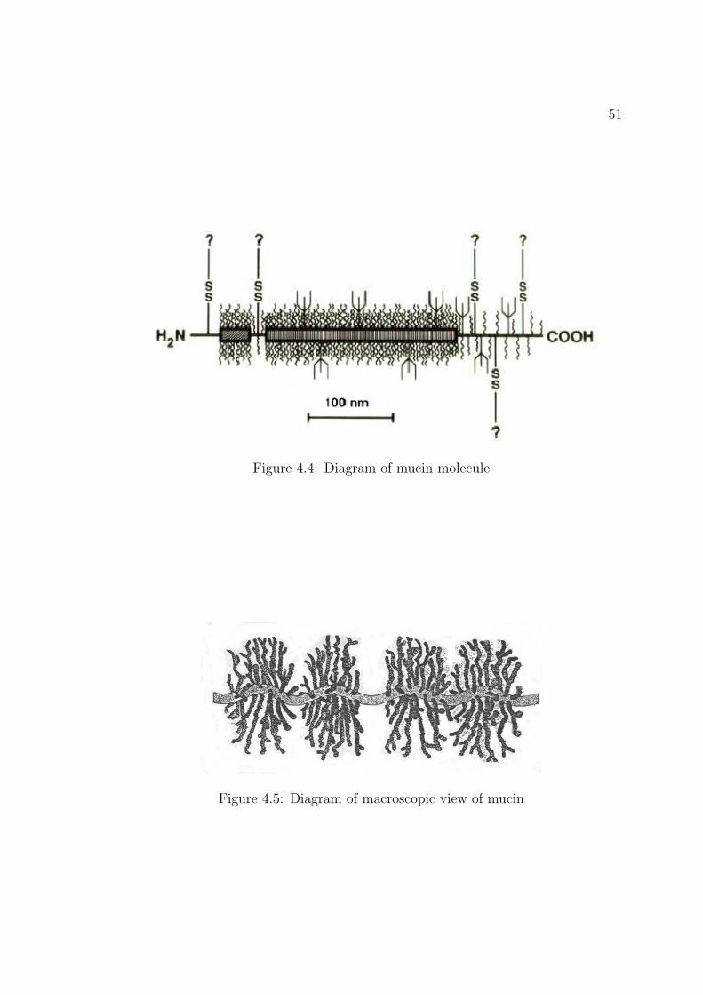
51
Figure 4.4: Diagram of mucin molecule
Figure 4.5: Diagram of macroscopic view of mucin

52
tions of mucus. These properties may also be implicated in the actions of the H.
pylori bacterium, which lives in the stomach and attaches to the stomach wall for
nourishment. H. pylori is implicated in ulcers and some types of stomach cancer
in humans. Previous dynamic light scattering studies of mucin demonstrated the
gel transition but were unable to obtain scattering data from the well-gelled state
due to very high turbidity. The microscope DLS system here is able to successfully
obtain light scattering data from the gel state due to the reduced scattering volume.
Additionally, tracer beads are used to estimate the pore size of the mucin gel and
to measure its bulk viscosity.
4.5 Mucin Protein Dynamics
Purified mucin was supplied by collaborators, in particular Brad Turner, at Beth
Israel Hospital. The mucin is purified by first scraping off the mucus layer of fresh
pig stomachs, and solubilizing the scrapings by stirring overnight in 0.2M NaCL
containing 0.04% sodium azide and the protease inhibitors benzamidine HCl, phenyl
methyl sulfonyl chloride, dibromoacetophenone, and EDTA adjusted to a pH of 7
with 1M NaOH. Centrifugation at 50,000 rpm for one hour removes coarse debris.
The supernatant containing soluble mucin is then fractionated in size by column
chromatography. Following fractionation, void volume fractions containing high
molecular weight periodic acid-Schiff (PAS) positive glycoproteins are pooled and
concentrated via ultrafiltration. The filter used has a cutoff of 300,000 Da. Purified
mucin is then prepared from the concentrate by density gradient ultracentrifugation
in CsCl with an initial concentration of 42% (w/w) at 300,000 rpm for 24 hours.
The densities of recovered fractions recovered from the tops of the tubes are then
determined by weighing aliquots and the glycoprotein content is determined by a

53
PAS assay. The fractions that contain glycoproteins of average density 1.45 g/ml
are then pooled, exhaustively dialyzed and lyophilized for further study33. When
the mucin is delivered from Beth Israel it is in solution form with a concentration
of 16.67 mg/ml. Buffers of varying pH are used to set the pH of the final solutions
that are studied.
Mucin has been previously studied using dynamic light scattering techniques3.
This study demonstrated that mucin undergoes a pH-induced gel transition near
pH 4 at a concentration of 10 mg/ml and higher. DLS measurements of the well-
gelled regime are difficult due to the high turbidity of the sample. At the gel point,
a power-law dependence of the structure factor is observed due to the divergence
of length scales within the material. Above the gel point the mucin was observed
to behave as a semi-dilute polymer, with interacting clusters. The hydrodynamic
radius of the mucin was determined to be 45 nm.
The microscope DLS system described here functions best with samples that
scatter very strongly due to the small scattering volume. Conversely, samples that
have adequate scatter for standard DLS can scatter much too weakly for the micro-
scope DLS system to measure. A concentration of 12 mg/ml was selected to insure
that the mucin would be in the well-gelled regime at pH 2. The samples of pH 6
mucin at this concentration did not yield any data beyond the noise floor of the
instrument due to the low inherent scatter. Initially, 109 nm beads were added to
the mucin as tracer particles with the intention of measuring the diffusion constant
of the gel and solution states. The results of the scattering at pH 6 with 109 nm
beads are shown in figure (4.6). The slight bump around 106µs on some of the
curves is an artifact of the correlator. For all the mucin measurements a 1 mW
HeNe laser at 635.2 nm was used. The green HeNe described previously was not
used until the unfortunate and unpredicted early demise of the red laser. There is

54
102
103
104
105
106
107
108
0
0.1
0.2
0.3
0.4
0.5
0.6
0.7
0.8
0.9
1
g(2) (τ
)−1
time µsec
Figure 4.6: 109 nm beads (1% v/v) in 12 mg/ml ph 6 mucin
some variation in the data here, but since the analysis method for nonergodic data
is intended for gel samples in which particles are trapped this method will not be
applied here. The variations in the data are rather the result of experimental error,
which is verified by comparing the ensemble averaged scattering intensity with the
local time averaged scattering intensity. For each of these sets of data this number
is very close to 1.
The expected shape of the structure factor as predicted by mode coupling the-
ory34 is of the form:
S(q, t) =
√G(2)(τ)−B
G(2)(0)−B= A exp(−t/τf ) + B exp(−(t/τs)
β) (4.14)
The first term is the short time dynamics, which reflects fluctuations in the density of
the solution. The second is a stretched exponential that characterizes the interaction
of the polymer clusters. The stretched term β where 0 ≤ β ≤ 1 is called the
width of the distribution and characterizes the polydispersity of the system. A

55
102
103
104
105
106
107
108
10−5
10−4
10−3
10−2
10−1
100
101
time (µsec)
−ln(
S(q
,t)Slope = β
Figure 4.7: Applying a stretched exponential to the 109 nm beads in pH 6 mucin
perfectly monodisperse system would have β = 1. Mode coupling theory makes
the general assumption that the system being studied is comprised of “basic units”
which interact in a strong nonlinear manner with each other. Long and short time
interactions are separated by a crossover time tc. For short times, t < tc, the units
relax independently following the fast exponential term of equation (4.14). The
stretched exponential term takes over at long times where t > tc. Attempts to fit
equation (4.14) with both the fast and slow terms to the data were not successful.
Only the second term, the slow dynamics term, results in an adequate fit to the
data. Figure (4.7) is a log− log plot of − ln(S)vs.t, where the slope of the plot gives
the value for β. Mode coupling theory associates τs ↔ Dq2 once β is determined34
for diffusive behavior. The average value for β here is 0.70 ± 0.05. Continuing the
fit to determine τs, a mean value of τs = 1.6× 10⁻⁶µsec is found. The dependence
of τs on the scattering angle was not investigated due to the limited range available

56
on the microscope. The average relaxation time is calculated as35:
〈τs〉 =
∫ ∞
0
e(−t/τs)β
dt =
(τs
β
)Γ
(1
β
)(4.15)
where Γ(x) is the gamma function. This yields 〈τs〉 = 2.9 × 10⁻⁶ seconds which
corresponds to a measured viscosity for the pH 6 mucin of 2 centipoise which is 2x
greater than the viscosity of water. The beads themselves are quite monodisperse,
but they are interacting with a set of polysdisperse polymer clusters, which may
explain why β < 1. Since the bead scattering data only fits the stretched exponential
fit, the concentration fluctuations in the sample may not be of sufficient amplitude
to have a measurable effect on the bead dynamics, which is why the fast term of
equation (4.14) is not observed.
An alternative interpretation of the stretched exponential is a model of micro-
scopic cages trapping the particles36. The cage size of the polymer solution can also
be estimated from this data with a re-write of S(q,t). Here, S(q,t) is a function of
the mean square displacement of the particles in the gel37:
S(q, t) = e−〈∆r2〉q2
6 (4.16)
The value of β indicates a scaling relationship with 〈∆r2〉 ∼ t0.7. Applying this
analysis to this set of scattering data gives an approximation of the cage size with
h =√〈∆r2〉. Here the cage size d = h+a where a is the bead radius and h the size
of the fluid filled gap between the bead and the wall of the cage. This is plotted in
figure (4.8). The mean value is d = 754± 323 nm. While no angle-resolved studies
were done due to the limited range of forward scattering angles that the instrument
is capable of measuring, it is worth nothing that the angle-dependent structure
factor is related to the correlation length of the system ξ by an Ornstein-Zernike

57
0 2 4 6 8 10 12 14
x 106
0.1
0.2
0.3
0.4
0.5
0.6
0.7
0.8
0.9
1
1.1
time µsec
cage
siz
e µm
Figure 4.8: Cage size of ph 6 polymer solution in microscopic cage model
equation38:
S(q) =I(q)
I(0)=
1
1 + (qξ)2(4.17)
The scattering data from the pH 2 mucin is quite different due to the gelation of
the sample. Here a modest amount of Triton X-100 (0.25%) was used to prevent the
mucin from sticking to the polystyrene tracer beads. Previous studies of other types
of mucin such as human cervical mucin and bovine submaxillary gland mucin have
shown that mucin molecules stick very readily to polystyrene39 40. The scattering
from the pH 2 mucin was weak but still must be accounted for in the data analysis.
Several autocorrelation curves were obtained from the mucin itself, along with a
mixture of mucin, 109 nm beads, and the Triton surfactant. Figure (4.5) shows
the autocorrelation curves from the pure mucin sample at 12 mg/ml along with an
average curve with error bars to show the general trend. The blue curve in figure
(4.9(a)) is quite anomalous in comparison to the rest of the data, and may have
been due to scattering from dust or other contaminates in the sample. The data

58
101
102
103
104
105
106
107
1
1.5
2
2.5
µsec
g(2) (τ
)
(a) Scattering from pure mucin at pH 2
101
102
103
104
105
106
107
0
0.2
0.4
0.6
0.8
1
1.2
1.4
µsec
g(2) (τ
)
(b) Average plot of data showing variation at shorttimes
at short time scales is very noisy due to the weak scattering and high noise level
which prevents analysis in this region. The variations in the g(2)(τ) curve for longer
times (> 1 sec) indicate nonergodicity in this case, since not only do they follow
different curves but in un-normalized form have widely varying scattering intensities,
as would be expected from a non-homogeneous gel. In contrast with the scattering
signal from the 109 nm beads, here the curves do not reach a baseline. The data
is fit to a sum of two functions, a power law and a stretched exponential. The gel
dynamics are expected to follow a power law near the gelation point changing to a
stretched exponential far from the gelation point. Since this transition is gradual,

59
the following form for S(q,t) was used:
S(q, t) = A(1 + t/τ0)−α + (1− A)e−(t/τ)β
. (4.18)
This fit is shown in figure (4.9). The amplitude of the power law fit is very small
with 〈A〉 = 0.07. The other parameters are 〈β〉 = 0.98, 〈α〉 = 0.26, and 〈τ〉 = 3.5
seconds.
The addition of 109 nm beads to the pH 2 mucin shows the a near-exponential
decay at short times followed by a rapid drop-off in g(2)(τ) at longer times. Since the
beads scatter more strongly than the mucin, they dominate the scatter at shorter
time scales until a time scale is reached where their motion is not longer correlated,
at which point the background mucin scatter dominates. This is illustrated in figure
(4.10). Since the autocorrelation signal of the beads themselves are the interest here,
the curves are cropped and only times which t < 5 sec are considered. This plot
illustrates the nonergodic nature of the bead dynamics in the gelled mucin. They
do not show very strongly nonergodic dynamics as has been previously observed28,
but the mucin gel is fairly soft and should contain a large degree of water, which
will allow for more movement and diffusion of the small 109 nm beads. The analysis
method by Pusey, et. al.27 for a single nonergodic process was the initial approach
taken to estimating the diffusion constant of the beads inside the gel. Briefly, the
process involves a factor relating the ensemble intensity average to the time intensity
average:
Y =〈I(q)〉E〈I(q)〉t
(4.19)
along with a factor involving the mean square value of the time intensity measure-
ment:
σ2I =
〈I2(q)〉t〈I(q)〉2t
− 1. (4.20)

60
101
102
103
104
105
106
107
10−4
10−3
10−2
10−1
100
101
µsec
−ln(
S(q
,τ))
105
106
107
10−4
10−3
10−2
10−1
100
101
−ln(
S(q
,τ))
µsec
Figure 4.9: Power law plus stretched exponential plot of pH 2 mucin

61
102
104
106
108
0
0.2
0.4
0.6
0.8
1
time (µsec)
g(2) (τ
)
Figure 4.10: 109 nm beads in pH2 mucin
A new structure factor is then calculated from the normalized intensity autocorre-
lation function as:
S(q, τ) =Y − 1
Y+
√g(2)(q, τ)− σ2
I
Y. (4.21)
Following this, a Taylor expansion of S at short times is done to derive a local
diffusion constant D. The apparent bulk diffusion constant DA is related to this as:
DA =DY
σ2I
. (4.22)
For one selected curve, the results for these calculations are Y = 0.8811 and σ2I =
0.0083, which leads to diffusion constant values of D = 8.8× 10⁻¹² and DA = 9.4×10⁻¹⁰. The corresponding microscopic viscosity from the Stokes-Einstein relation
is .45 centipoise, which is less than water, and the bulk viscosity is 4.2 × 10⁻³
centipoise. For comparison, the viscosity of distilled water at 20 is 1 centipoise. It
is expected that the beads will tend to see a varying viscosity inside the gel due to
62
0 100 200 300 400 500 600 700 800 900 10000.95
0.96
0.97
0.98
0.99
1
1.01
time (µsec)
S(q
,t)
slope=−4.338371e−005
corrected data1st order fit
Figure 4.11: Short-term fit to the structure factor with nonergodic corrections
interactions between the beads and the mucin molecule. However, the macroscopic
viscosity is over 200× lower than that of water! These results illustrate the necessity
of correcting for the scattering effects of the gel on the signal when the scattering
intensity of the tracer beads is close to that of the gel. The short term fit of the
structure factor corrected for nonergodic effects is shown in figure (4.11). Continuing
the analysis of this data a mean value for the microscopic diffusion constant of 0.39×10⁻¹¹ ± 0.1 × 10⁻¹⁰ is found, with a corresponding viscosity of 1.3 ± 0.6centipoise.
The results are summarized in table 4.5. This result indicates that the microscopic
viscosity of well-gelled porcine gastric mucin at room temperature is somewhat
higher than that of water at room temperature.
4.6 Matrigel
Matrigel is a commercial basement membrane that is commonly used in culturing
cells, in particular tumor cells. A basement membrane is a type of extracellular

63
Data Y σ2I D(m2/s) η(centipoise)
A 1.55 0.127 0.36× 10⁻¹¹ 1.51B 1.04 0.008 0.51× 10⁻¹¹ 0.74C 1.15 0.004 0.57× 10⁻¹¹ 0.74D 0.88 0.008 0.62× 10⁻¹¹ 0.64E 1.56 0.176 0.61× 10⁻¹¹ 1.09F 2.25 0.083 0.24× 10⁻¹¹ 2.26G 2.15 0.052 0.23× 10⁻¹¹ 1.93
mean 0.39× 10⁻¹¹ 1.3
Table 4.1: Summary of 109 nm beads in mucin
matrix that underlies epithelial layer cells and helps them to adhere to the tissue
below. Epithelial layer cells make up the epithelium, which is membranous tissue
covering internal organs and other internal surfaces of the body. First patented in
1989, Matrigel has seen wide success and the original paper41 has been cited hun-
dreds of times. According to the literature from the manufacturer, BD Biosciences,
Matrigel is extracted from the EHS mouse tumor which is rich in basement mem-
brane proteins. The major matrix components are laminin, collagen I, entactin,
and heparan sulfate proteoglycan42. The matrix also contains growth factors, ma-
trix metalloproteinases, and other proteinases43, as well as several undefined com-
pounds44. Matrigel does not contain any detectable levels of tissue inhibitors of
metalloproteinases which act to inhibit the growth of tumor cells43. To date there
have not been any studies of the viscoelastic properties of Matrigel and whether or
not this is relevant to the behavior of cells grown on or in the gel. It is clear that the
mechanical substrate properties do effect cell growth behavior5 45 46 since cells will
grow very different on a squishy gel compared with a glass dish. The particular cell
type being grown also determines the an appropriate substrate stiffness. Nerve cells,
for example, grow very poorly on glass surfaces (infinite stiffness, as far as the cell
is concerned), but show increased branching and growth on squishy polyacrylamide

64
with an elastic modulus of 500 dyn/cm2 5.
4.7 Matrigel Dynamics
In order to study the properties of Matrigel, fresh samples were obtained from both
collaborators and from the manufacturer. BD Biosciences makes claims for a high
level of consistency between batches of Matrigel so this should not be a factor.
Three sizes of polystyrene tracer beads were used with diameters of 109 nm, 510
nm, and 2 micron. Additionally, scattering data from the gel itself was obtained. All
experiments were done at room temperature. The standard preparation of Matrigel
is quite straightforward. It is kept frozen until use, at which point the sample is
allowed to thaw overnight in an ice bath, preferably at 4. The sample is then
pipetted onto a slide, incubated at 37for at least 30 minutes, and then cooled to
room temperature. The slides are pre-cleaned with a mixture of isopropyl alcohol
and potassium hydroxide, which etches the glass clean. After cleaning the slides
are washed with Millipure filtered distilled water, which is also used for diluting
the bead solution. The Matrigel will remain in a gel state as long as it is not
re-frozen. Pre-diluted beads and Triton X-100 are added to the Matrigel prior
to pipetting. The Triton X-100 serves to prevent clumping of the beads in the
mixture. The general recipe used is 50 µL of Matrigel, 10 µL of bead solution,
and 0.5 µL of undilute Triton. The bead solution is pre-diluted so that the final
solution has the desired bead concentration. For the 2.03 micron beads, this is
0.01% by volume. Beads of this size appear to be just about at the upper limit for
use in the light scattering microscope. At this concentration and full laser power
the scattering counts at 11.32°is only about 45,000 counts per second. Figure (4.12)
shows normalized structure factor from these beads at this concentration with a fit

65
10−4
10−2
100
102
0
0.2
0.4
0.6
0.8
1
1.2
1.4
sec
S(q
,τ)
2.03 µm beads at 0.01%
Calculated diameter: 1.89 µm
Figure 4.12: Autocorrelation of 2.03 µm beads
from a single exponential.
The normalized structure factor is calculated as:
S(τ) =
√G(2)(τ)−B
G(2)(0)−B(4.23)
where B is the baseline the autocorrelation signal G(2)(τ) has decayed to. The final
concentrations for the 510 nm and 109 nm beads were 0.33% and 0.3% by volume,
respectively, and the concentration of Matrigel was 84%. Matrigel is frequently
diluted in use, so this level of dilution should result in applicable results.
After the Matrigel had polymerized, the samples were placed on the microscope
stage, a spot was picked for scattering, and data was collected for 30 minutes. After
this the sample was translated and the measurement repeated. The Pusey method
of correcting for nonergodic dynamics requires an ensemble average of the scattering
intensity, so this was also collected by manually translating the sample on the stage
while recording a count rate history using the software for the BI-9000 correlator.

66
102
104
106
108
0
0.2
0.4
0.6
0.8
1
µsec
g(2) (τ
)−1
data 1data 2data 3data 4data 5
Figure 4.13: Scattering of pure Matrigel
4.7.1 Pure Matrigel
Figure (4.13) shows several runs from the pure Matrigel. The autocorrelation signal
has been normalized to the first data point. The wiggle in the data at around 105µsec
is a systematic error in the system that is only observed when the scattering signal
is very weak. Some areas of the Matrigel scattered more strongly than others, which
indicates that while the solution may be uniform and consistent in its formulation
the polymerization of the Matrigel is not necessarily uniform across the sample.
These autocorrelation curves have two interesting portions. There is a short-time
exponential decay which is frequently associated with concentration fluctuations in
the sample. However, in this case this appears to be due to some high-frequency
noise in the laser system, so this fast time decay will be ignored in the analysis. The
long-term drop off in the scattering signal is frequently observed in gel samples, and

67
2 3 4 5 6 7 8−2.5
−2
−1.5
−1
−0.5
0
0.5
log10
(µsec)
log 10
(−lo
g(S
))
β=0.14
Figure 4.14: A stretched exponential fit to S(q,τ) for pure Matrigel
is best fit by a stretched exponential of the form:
G(2)(τ) = Ae−(τ/τc)β
. (4.24)
Figure (4.14) shows the fit to this equation at the longer times for the measurement
for the highest scattering signal, with β = 0.14 which is a good fit to the data over
four and a half decades in time. The low value of β indicates a wide variety of length
scales in the gel. The electron micrograph in the original paper41 indicates that the
crosslinking in Matrigel is very non–uniform.
4.7.2 109 nm beads in Matrigel
Figure (4.15) shows the normalized autocorrelation signal and the structure factor
S(q, t) for the 109 nm beads added to the matrigel. The normalized autocorrela-
tion signal does not quite decay to a baseline by τ = 1sec, which is indicative of

68
102
103
104
105
106
1
1.1
1.2
1.3
1.4
1.5
1.6
1.7
1.8
1.9
2
time (µsec)
g(2) (τ
)
Figure 4.15: g(2)(τ) for 109 nm beads in Matrigel
subdiffusive behavior in which the beads do not freely move about the sample. Due
to the very weak scattering from the Matrigel this data does not benefit from the
dual nonergodic process analysis detailed in section 3.4.1. The single nonergodic
analysis is certainly applicable in this case. Applying this method to the results in
the values in table 4.7.2. The 109 nm beads are evidently small enough to diffuse
about the pores of the Matrigel and experience a viscosity identical to that of water
Data Y σ2I D (m2/s) η (centipoise)
A 0.88 0.009 4.61× 10⁻¹² 0.9B 1.03 0.003 4.53× 10⁻¹² 0.9C 1.20 0.005 3.88× 10⁻¹² 1.0D 1.54 0.009 3.61× 10⁻¹² 1.1E 1.03 0.014 3.29× 10⁻¹² 1.2F 1.31 0.004 4.02× 10⁻¹² 1.0G 0.89 0.005 5.13× 10⁻¹² 0.8
mean 4.15× 10⁻¹² ± 6.4× 10⁻¹³ 1.0± 0.2
Table 4.2: Summary of 109 nm beads in Matrigel

69
at room temperature. This is confirmed by plotting the mean square displacement
of the 109 nm beads which confirms that the MSD increases linearly with time from
0.1 ms to 15 ms. Since Matrigel contains a variety of chemical factors that promote
cell growth, it is concluded that these constituents can be expected to diffuse about
in a similar fashion.
If the tracer beads are large enough that they experience essentially a uniform en-
vironment, then the microrheological approach can be used to analyze the data. The
corrections for nonergodicity still apply, but instead of investigating the diffusion
constants the mean square displacement will be analyzed to compute the complex
shear modulus of the bead dynamics. Since Matrigel is used to culture cells which
generally move slowly, the quantity of most interest will be the low frequency shear
modulus G which is calculated from2:
〈∆x2〉 =kBT
πrG(4.25)
where the value on the left hand side is the saturation value of the mean square
displacement at long times. In order to avoid the calculation of a numerical forward
Laplace transform in the calculation of the complex shear modulus and its associated
inaccuracies at the lowest and highest times, a power law approximation will be
made47:
G(s) ≈ kBT
πr〈∆r2(t)〉Γ(1 + α)(4.26)
where the function α is:
α =∂ log 〈∆r2〉
∂ log t(4.27)
and Γ is the gamma function.
Two sizes of tracer beads were used for this study. The sizes were 2.03 µm and

70
Figure 4.16: A bead trapped in a gel network
510 nm diameter polystyrene beads. Unlike the smaller 109 nm beads, the larger
sizes needed higher quantities of the Triton surfactant added to prevent the beads
from sticking to the Matrigel. Even at a Triton concentration of 1% by volume, the 2
µm beads bonded to the Matrigel. The resulting autocorrelation curve showed only
the stretched exponential behavior observed in the pure sample, which indicates that
the beads were stuck to the gel network and moving with it. The desired situation
is illustrated in figure (4.16). In Matrigel the situation is further complicated by
the wide variety of pore sizes (as high as 200 µm) as was shown in an electron
micrograph in the original paper on the material41. To account for this distribution
in pore sizes measurements incorporating a variety of beads sizes would be ideal.
The 510 nm beads had a modest degree of success. Here the 1% Triton by volume
allowed the beads to move within the network, although after several hours the
beads still stuck to the gel network, resulting in the autocorrelation signal taking
on the recurring stretched exponential form. Figure (4.17) shows the mean square

71
103
104
105
106
10−7
10−6
time (µsec)
<∆r2 >1/
2 (cm
)
ABCD
Figure 4.17: Mean square displacement of 510 nm beads in Matrigel
displacement of the beads in the Matrigel, calculated according to the relation
S(q, τ) = e−q2〈∆r2(τ)〉/6. (4.28)
The time data is cropped below 1 millisecond due to laser noise which caused an
oscillation in the short-time autocorrelation function b. Two of the curves saturate
at long times, which allows for the calculation of the low-frequency elastic shear
modulus as
G =kBT
πr〈∆x2(τ)〉 (4.29)
where 〈∆x2(τ)〉 = 〈∆r2(τ)〉/3. The mean value of G from these two measurements
is 50.2± 6.0dynes/cm2. Since the elastic shear modulus characterizes the ’rigidity’
of the gel, this indicates a very soft and squishy gel, which agrees with qualitative
bThe original red HeNe laser worked well. Switching to the green HeNe after the demise ofthe red one gives an advantage in the scattering efficiency due to the shorter wavelength, butthe particular green HeNe used has some high frequency noise that causes trouble for short-timemeasurements. This noise may be correctable through power supply improvements.

72
observation of the sample. A published study of neurite branching5 on polyacry-
lamide gels used a shear modulus of less than 500 dynes/cm2 at the low end of the
range of shear moduli studied. The pure Matrigel will have a higher value for G
than was measured here due to the higher concentration of crosslinking polymers
and the elimination of any softening effects from the Triton surfactant. The large
difference in the autocorrelation functions between the two curves that saturate and
the two that don’t deserve some comment. Due to the wide variety of pore sizes, in
some areas the pore size is likely to have been in the regime where it is similar to
the bead size, which will not accurately reflect the rheological properties of the gel.
The success of studying the motion of the 109 nm beads and the tendency of the 2
µm beads to stick to the gel suggests that the pore size is typically in between these
limits. It is concluded that at least a portion of the success of Matrigel as a substrate
for cell growth is due to its favorable mechanical properties which are comparable
to real tissue48. The DLS microscope is also capable of making microrheological
measurements of very small quantities of material, provided attention is paid to the
number and the motility of the tracer particles.
4.8 Conclusions
The design and construction of a DLS microscope achieved its goals. The instru-
ment has a small scattering volume of approximately 10 nL, a selectable scattering
volume using the microscope optics, and a well-defined scattering angle. This in-
strument improves upon the initial design by Prof. David Weitz’s group at Harvard
in its calibration and its ease of use. The small scattering volume allows for the
observation of nonergodic dynamics in appropriate samples and additionally rhe-
ological parameters can be measured using microspheres as tracer particles. The

73
DLS microscope has proven effective for studying polymers and gels for biological
applications.
The porcine gastric mucin (PGM) glycoprotein is a large molecule that is the
principal component of the mucus layer lining the stomach in pigs. In general, the
viscoelastic properties of mucin allow for the lubricative and protective properties of
the mucus layer. The PGM was studied at pH 2 and pH 6 both by scattering from
the pure mucin and by scattering from embedded 109 nm polystyrene microspheres.
At pH 6 the mucin is in a semidilute polymer solution, and the pure solution did not
provide enough scattering for measurement with the DLS microscope. The addition
of the polystyrene microspheres allowed for the measurement of stretched exponen-
tial behavior in the bead dynamics with the stretching exponent β = 0.7pm0.05.
The microspheres experience a viscosity twice that of water in the semidilute poly-
mer solution. At pH 2 the mucin forms a gel, and scattering from the pure gel shows
dynamics that follow a power law with an exponent α = 0.26 and an amplitude of
only 0.07, along with a dominating stretched exponential with the stretching expo-
nent β = 0.98. The autocorrelation function from scattering off of the polystyrene
microspheres displays nonergodic dynamics. The theoretical method by Pusey, et.
al. allows for the analysis this data to dertermine the microviscosity experienced by
the beads. This microviscosity is 1.3× greater than water.
Matrigel is a commercial basement membrane which was also studied with the
light scattering microscope. Again, the pure gel, after preparation following the
manufacturer’s instructions, showed stretched exponential behavior with β = 0.14.
The 109 nm microspheres in Matrigel experience a microviscosity identical to that
of water at room temperature, indicating that the components that make up the
gel are not interacting with the beads in a significant manner. 510 nm beads were
also added to the Matrigel and their dynamics were analyzed in terms of their mean

74
square displacement to yield an estimate of the low-frequency elastic shear modulus
with a value of 50.2± 6.0 dynes/cm2.

Chapter 5
Raman Scattering
5.1 A Brief History of the Raman Effect
The Raman effect, which is light scattering by vibrational modes in molecules, was
discovered in 1928 by C.V. Raman49 using sunlight as the light source, a telescope
as the collector, and eyeballs as the detector. After placing a filter in the sunlight to
reduce the bandwidth of the illumination, a second filter of longer wavelength was
placed next to a liquid sample and scattered light was observed. Over the subsequent
decades, much progress was made in light sources and detection methods that served
to make Raman scattering spectroscopy a very useful tool in the laboratory. Systems
employed today typically use laser light for illuminating samples, and either triple
monochromators and photomultiplier tubes or dispersion gratings and CCD chips
for detection. This chapter introduces the basics of the Raman effect in the context
of simple molecules. A full detailed description of the Raman effect is beyond the
scope of this thesis.

76
Figure 5.1: C.V. Raman
5.2 Classical Raman Scattering Theory
Raman scattering can be adequately described by classical electrodynamics and
mechanics, although the complete description requires the use of quantum mechanics
and group theory. This section describes vibrational scattering from classical theory
in the case of a single diatomic molecule. If two atoms of masses m1 and m2 are
connected by a chemical bond and are separated from the center of gravity by
distances r1 and r2, then the relationship m1r1 = m2r2 holds true. If the the masses
are displaced slightly by x1 and x2 from their equilibrium positions, m1(r1 + x1) =
m2(r2 + x2) is also true.
Combining these equations gives:
x1,2 =
(m2,1
m1,2
)x2,1 (5.1)
The chemical bond can be modeled as a spring joining the two atoms that obeys

77
Hooke’s Law, so that the restoring force F with spring constant K is
F = −K(x1 + x2) (5.2)
Combining the spring force with equation (5.1) gives
F = −K
(m1,2 + m2,1
m1,2
)x2,1 (5.3)
Applying Newton’s equation F = ma for each atom results in
m1d2x1
dt2= −K
(m1 + m2
m2
)x1 (5.4)
m2d2x2
dt2= −K
(m1 + m2
m1
)x2 (5.5)
(5.6)
which leads to
m1m2
m1 + m2
(d2x1
dt2+
d2x2
dt2
)= −K(x1 + x2). (5.7)
The reduced mass µ and displacement q can be applied here to simplify this equation
to
µd2q
dt2= −Kq. (5.8)
This differential equation is easily solved as
q = q0 sin(2πν0t + φ) (5.9)
where q0 is the maximum displacement and φ is a phase term. ν0 is the classical

78
vibrational frequency
ν0 =1
2π
√K
µ(5.10)
This is, of course, the equation of motion for a harmonic oscillator, whose full
dynamics are described in typical physics textbooks.
As was described previously, Raman spectra arise from the interaction of incom-
ing photons with the vibrational modes of the molecule. The incoming light is in the
UV-visible range, and will scatter either elastically (Rayleigh) or inelastically (Ra-
man). The Raman scattering is very weak, typically ≈ 10−6− 10−5 of the incoming
beam and has frequencies ν0±νm where ν0 is the frequency of the incoming light and
νm is the vibrational frequency of the molecule. The Raman scattered light is ob-
served experimentally to have a spectrum of discrete, narrow lines both higher and
lower in energy with respect to the irradiating light. The photons of higher energy
are called the anti-Stokes lines and the lower energy photons the Stokes scattered
lines.
Using classical theory, the Raman scattered photons can be explained in terms
of an interaction between the incoming electric field E and the polarizability α of
the molecule. The electric field of the irradiating light has a field strength that
fluctuates as
E = E0 cos(2πν0t) (5.11)
where E0 is the amplitude and ν0 the laser frequency. An electric dipole P is induced
as
P = αE = αE0 cos(2πν0t). (5.12)
If the molecule vibrates with frequency νm then the center-of-mass displacement q
is
q = q0 cos(2πνmt) (5.13)

79
where q0 is the vibrational amplitude. For a small perturbation of q, this can be
linearly expanded in α:
α = α0 +
(∂α
∂q
)
0
q0 + · · · (5.14)
Combining equations (5.12), (5.13), and (5.14) gives
P = αE0 cos(2πν0t)
= α0E0 cos(2πν0t) +
(∂α
∂q
)
0
qE0 cos(2πν0t)
= α0E0 cos(2πν0t) +
(∂α
∂q
)
0
q0E0 cos(2πν0t) cos(2πνmt)
= α0E0 cos(2πν0t) +1
2
(∂α
∂q
)
0
q0E0[cos(2π(ν0 + νm)t)
+ cos(2π(ν0 − νm)t)]. (5.15)
The first term in equation (5.15) represents an oscillating dipole radiation light of
frequency ν0 (Rayleigh scattering), the second term is radiation at frequency ν0+νm
(anti-Stokes scattering), and the third term is radiation at frequency ν0−νm (Stokes
scattering). If the change in the polarizability is zero, then that vibration is not
Raman active.
This treatment provides the essentials of predicting the frequency of Raman scat-
tered light. The procedure to do so involves applying the classical selection rules
for vibrational frequencies to the molecule of interest12. This becomes progressively
more difficult as the complexity of the molecule increases. Homonuclear diatomic
molecules, written as A2a, have just one mode of vibration. These molecules have
no net electric dipole, and the electron symmetry does not change for small pertur-
bations of the relative atomic positions, so these molecules are not infrared active.
The polarizability is non-zero, and can be considered in two directions: parallel to
ae.g. molecular hydrogen H2
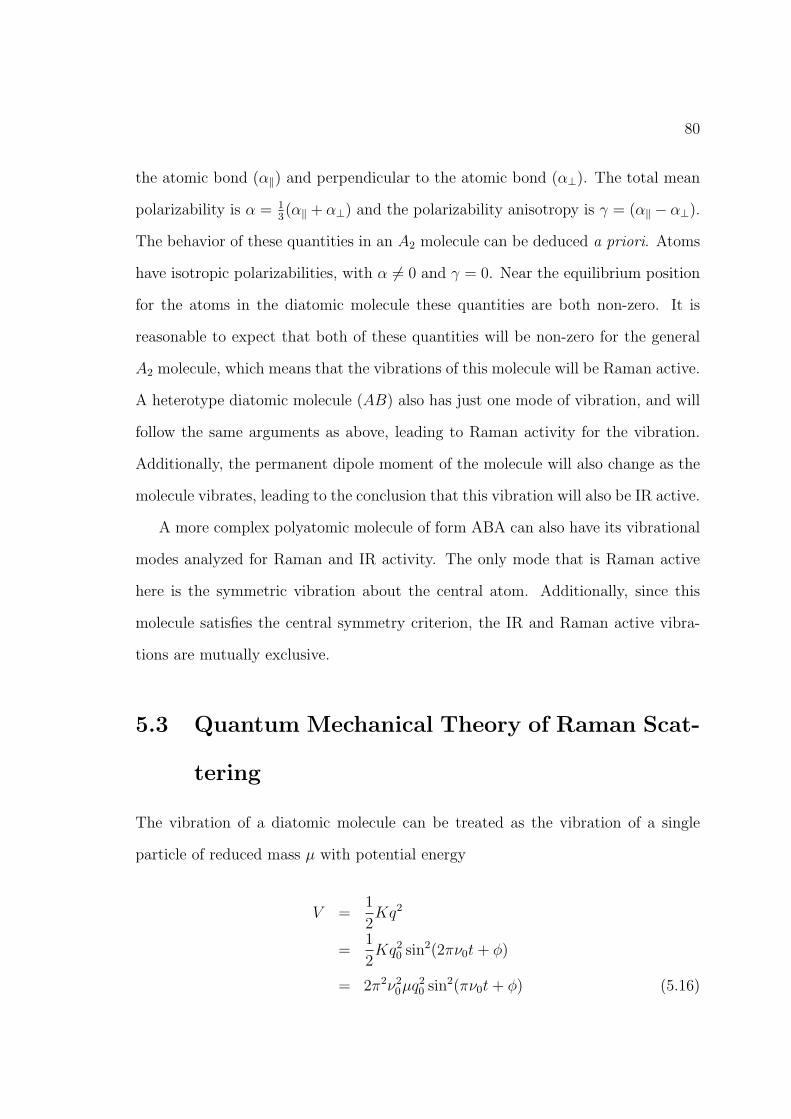
80
the atomic bond (α‖) and perpendicular to the atomic bond (α⊥). The total mean
polarizability is α = 13(α‖ + α⊥) and the polarizability anisotropy is γ = (α‖ − α⊥).
The behavior of these quantities in an A2 molecule can be deduced a priori. Atoms
have isotropic polarizabilities, with α 6= 0 and γ = 0. Near the equilibrium position
for the atoms in the diatomic molecule these quantities are both non-zero. It is
reasonable to expect that both of these quantities will be non-zero for the general
A2 molecule, which means that the vibrations of this molecule will be Raman active.
A heterotype diatomic molecule (AB) also has just one mode of vibration, and will
follow the same arguments as above, leading to Raman activity for the vibration.
Additionally, the permanent dipole moment of the molecule will also change as the
molecule vibrates, leading to the conclusion that this vibration will also be IR active.
A more complex polyatomic molecule of form ABA can also have its vibrational
modes analyzed for Raman and IR activity. The only mode that is Raman active
here is the symmetric vibration about the central atom. Additionally, since this
molecule satisfies the central symmetry criterion, the IR and Raman active vibra-
tions are mutually exclusive.
5.3 Quantum Mechanical Theory of Raman Scat-
tering
The vibration of a diatomic molecule can be treated as the vibration of a single
particle of reduced mass µ with potential energy
V =1
2Kq2
=1
2Kq2
0 sin2(2πν0t + φ)
= 2π2ν20µq2
0 sin2(πν0t + φ) (5.16)

81
The Schrodinger equation for this system is50
d2ψ
dq2+
8π2µ
h2
(E − 1
2Kq2
)ψ = 0 (5.17)
The solution to this equation, with the constraint that the wave equation ψ be
single-valued, finite, and continuous, is:
Eν = hν
(ξ +
1
2
)= hcν
(ξ +
1
2
)(5.18)
with the frequency of vibration ν
ν =1
2π
√K
µ(5.19)
ν =1
2πc
√K
µ(5.20)
The quantity ξ is the quantum number with the integer values 0, 1, 2, . . .. The wave
function ψ is
ψξ =(α/π)1/4
√2νξ!
e−αq2/2Hξ(√
αq) (5.21)
where
α = 2π
õK
h(5.22)
and Hξ(√
αq) is the Hermite polynomial of the ξth degree. The frequency of vi-
bration is the same as for the classical derivation. The lowest energy state has
an energy of 12hν, and the selection rules only allow transitions of ∆ν = ±1. Di-
atomic molecules do not quite follow a harmonic oscillator potential, but are better

82
Morse PotentialHarmonic Oscillator
Figure 5.2: The Morse and harmonic oscillator potentials
described by the Morse potential:
V = De
(1− e−βq
)2(5.23)
where De is the disassociation energy of the molecule and β measures the curvature
of the potential at its lowest points. The eigenvalues of this potential from the
solution of the Schrodinger equation are:
Eν = hcωe
(ν +
1
2
)− hcχeωe
(ν +
1
2
)2
+ . . . . (5.24)
The quantity ωe is the wavenumber with corrections for anharmonicity, and χe
is the degree of anharmonicity. The two potentials are plotted for comparison in
figure (5.2). The selection rules weakly allow transitions of ∆ν = ±2,±3, . . . for
the anharmonic oscillator. The preceding discussion regarding the polarizability of
the molecule applies to the quantum mechanical case as well. In terms of electronic

83
Figure 5.3: Virtual energy levels
energy levels, incoming photon is exciting an electron to a virtual energy level, with
the initial and final energy levels of the photon determining whether the scattered
light is Stokes or anti-Stokes scattered. This is illustrated in figure (5.3).
5.3.1 Polarizability
Equation (5.12) is the basic equation for the polarizability P . The polarizability of
actual molecules involve vector quantities for both P and E, and equation (5.12)
can be re-written as:
Px = αxxEx + αxyEy + αxzEz
Px = αyxEx + αyyEy + αyzEz
Px = αzxEx + αzyEy + αzzEz (5.25)
This can also be written in matrix form:
Px
Py
Pz
=
αxx αxy αxz
αyx αyy αyz
αzx αzy αzz
Ex
Ey
Ez
(5.26)

84
Figure 5.4: CO2 and its polarizability ellipse
The matrix on the right-hand side is called the polarizability tensor. A molecular
vibration is Raman-active if one of the components of this tensor is changed during
the vibration. The CO2 molecule is typically used to illustrate the application of
this tensor to the determination of Raman activity. A plot of αi along the three
axes will generate a surface. Typically, the quantity 1/√
α is plotted and called
the polarizability ellipse. Figure (5.4) shows the polarizability ellipse for the three
vibrational modes of CO2. Of the three vibrational modes, only the first, v1, is
Raman-active. At positions ±q the shape of the polarizability ellipse is changing
along with all three diagonal elements of αij. For the other two modes, the shape of
the ellipse is the same at ±q, meaning there is no change for small vibrations. This
method is not applicable to more complex molecules. Group theory is needed to
describe the Raman activity of larger and more complex molecules. An explanation
of this application of group theory and the use of point symmetry elements is beyond

85
the scope of this thesis. A complete description can be found in the references51 12.
Briefly, the selection rule for Raman activity is found by solving a set of integral
equations:
(αxx)ν′,ν′′ =
∫ψ∗ν′(Qa)αxxψν′′(Qa)dQa
(αyy)ν′,ν′′ =
∫ψ∗ν′(Qa)αyyψν′′(Qa)dQa
(αzz)ν′,ν′′ =
∫ψ∗ν′(Qa)αzzψν′′(Qa)dQa
(αxy)ν′,ν′′ =
∫ψ∗ν′(Qa)αxyψν′′(Qa)dQa
(αyz)ν′,ν′′ =
∫ψ∗ν′(Qa)αyzψν′′(Qa)dQa
(αxz)ν′,ν′′ =
∫ψ∗ν′(Qa)αxzψν′′(Qa)dQa (5.27)
Here the αij′s are the components of the polarizability tensor. ψν′ and ψν′′ are the
vibrational wavefunctions where ν ′ and ν ′′ are the vibrational quantum numbers for
the initial and final states. Qa is the normal coordinate of the normal vibration a. At
least one of these integrals must be non-zero for the vibration to be Raman-active.
Symmetry considerations allow for the rapid determination of Raman activity, which
is where group theory is used to classify vibrations according to their symmetry
properties.
5.3.2 Resonance Raman Scattering
If there is an electronic energy level in a chromophoric group whose energy corre-
sponds to the excitation energy of an incoming photon, then the resulting Raman
intensities are selectively enhanced by a factor of about 103 to 105. If the incoming
photon has energy ν0 then the intensity Imn of a Raman band where m and n are

86
the initial and final states is52:
Imn = constant · I0(ν0 − νmn)4∑ρσ
| (αρσ)mn |2. (5.28)
I0 is the initial incoming intensity. The subscript e represents the virtual energy
level. The polarizability term (αρσ)mn can be re-written52 as:
(αρσ)mn =1
h
∑e
(MmeMen
νem − ν0 + iΓe
+MmeMen
νem + ν0 + iΓe
). (5.29)
Here, νem and νen are the energy differences between the states specified by the
subscripts. The Mij′s are the electric transition moments
Mij =
∫Ψ∗
i µσΨjdτ. (5.30)
Ψi and Ψj are the wavefunctions of the i and j states and µσ is the σth component
of the electric dipole moment. The factor iΓe is called the damping constant with
Γe the bandwidth of the virtual energy state. In normal Raman conditions, the
scattering intensity is dominated by the (ν0 − νmn) term. As the energy of the
illuminating radiation approaches νem, the scattered intensity rises dramatically.
5.4 Applications
Figure (5.5) shows the actual Raman spectrum of polystyrene. This spectrum was
measured on a commercial Raman spectrometer (Renishaw Corp.) using an argon-
ion laser at 488 nm. The rising background is due to intrinsic fluorescence in the
sample. This can typically be avoided through one of several ways, such as choosing
an excitation wavelength that does not excite the fluorescence (such as the near-

87
2750 2800 2850 2900 2950 3000 3050 3100 3150 32000.8
0.9
1
1.1
1.2
1.3
1.4
1.5
1.6
1.7
1.8x 10
5
cm−1
coun
ts
polystyrene bead Raman spectrum, 488nm excitation
Figure 5.5: Raman spectrum of polystyrene
infrared), or by illuminating the sample for a sufficiently long time that the sample
photobleaches. In the operation of the Raman microscope, images are recorded using
a bandpass filter set to the desired Stokes scattered wavelength. After acquisition,
the filter is tuned just off-peak and an additional image is recorded that contains
the fluorescence background. Image subtraction then removes the background.
Raman scattering spectroscopy is typically used for the identification and study
of molecules, as well as the study of molecular structure. Industries as varied as
the computer hard disc, pharmaceutical, polymer, semiconductor, and chemical
industries make use of Raman spectroscopy. Paint and pigments are also analyzed to
aid in the restoration of art, and forensic scientists make use of Raman spectroscopy
to aid in the identification of drugs and explosives. There are also a number of
medical studies involving Raman spectroscopy, for example to noninvasively identify
blood analytes and glucose concentrations53.
A typical experimental setup for the Raman effect involves the use of an illumi-

88
nating laser, a sample holder, a monochromator for isolation of a particular scattered
wavelength, and a photon detector. Frequently, a dispersive monochromator is used
with a CCD detector to simultaneously measure the entire desired spectrum, with
each column in the CCD detector corresponding to a different wavelength. Raman
microspectroscopy involves the marriage of an optical microscope to a Raman spec-
trometer. In this type of setup, the microscope objective focuses the illuminating
laser to a diffraction limited spot on the sample, and the scattered light is coupled
to the monochromator through the microscope optics. Spatial resolution is limited
to the Abbe resolution limit described in chapter 2.

Chapter 6
Total Internal Reflection
Microscopy Experiments
6.1 Imaging Past the Diffraction Limit
The limitations on the resolution of a microscope imposed by Fraunhofer diffraction
are described in chapter 2. Scanning electron and atomic force microscope have
resolutions far beyond optical microscopy, but are invasive or destructive to biolog-
ical samples. Increasing the resolution by decreasing the wavelength is of limited
practicality since biological samples are readily damaged by UV radiation, and the
numerical aperture of microscope objective lenses is limited by the availability of
high index of refraction immersion oils.
Various methods have been developed to improve the axial and lateral resolu-
tion of optical microscopy. Techniques such as confocal and two-photon microscopy
offer a modest improvement in resolution, and emerging techniques such as stimu-
lated emission depletion (STED) microscopy8 offer significantly higher resolution.
Methods involving interferometry include 4π microscopy, I5M 6 microscopy, har-

90
n2
n1
≥θC
x
z
Figure 6.1: Total Internal Reflection
monic excitation light microscopy (HELM)7, and standing wave total internal re-
flection microscopy11 where the first two improve the axial resolution and the latter
two the lateral resolution. Two techniques, near-field scanning optical microscopy
(NSOM)54 and the solid immersion lens10, make use of near field electromagnetic
and lens interactions to achieve high resolution.
6.2 Total Internal Reflection
Total internal reflection is the reflection of light from the interface between two
media of different refractive indices when the incident angle is greater than a critical
angle as shown in figure (6.1). The critical angle is θc = sin−1(n2/n1) when n2 <
n1. Solving Maxwell’s equations with the appropriate boundary conditions for an
incident plane wave shows that while the wave is completely reflected off the interface
there is an electric field in medium n223 although there is no energy transmitted
across the interface.

91
θ
θc z
x
Ez
Ex
Evanescent field
Figure 6.2: Electric fields in total internal reflection
6.2.1 The Evanescent Field
Under total internal reflection conditions, the electric field outside of the prism is
called the evanescent field. The details of the interference pattern formed by two
evanescent fields was originally developed in the interest of enhancing the routine
technique of total internal reflection fluorescence microscopy55. The electric field is
not purely a transverse wave since it has a longitudinal component in its direction
of travel and has the form:
E(r, t) = ReAE0(θ, α)ei(k(θ)x−ωt)
e−z/(2d(θ)) (6.1)
where the interface between the two media is in the x − y plane and the incidence
plane is the x− z plane, as shown in figure (6.1). The incident beam of frequency ω
and wavelength λ has an electric field amplitude of A that is polarized at an angle

92
α from the incident plane. The other quantities in equation (6.1) are defined as:
E0x = ax (θ) cos (α) e−i[δp(θ)+π/2] (6.2)
E0y = ay (θ) sin (α) e−iδs(θ) (6.3)
E0z = az (θ) cos (α) e−iδp(θ) (6.4)
ax = 2 cos (θ) X (θ)[(
sin2 (θ)− n2)1/2
](6.5)
az = 2 cos (θ) X (θ) [sin (θ)] (6.6)
ay =2 cos (θ)
(1− n2)1/2(6.7)
X (θ) =(n4 cos2 (θ) + sin2 (θ)− n2
)−1/2(6.8)
δs =tan−1
(sin2 (θ)− n2
)1/2
cos (θ)(6.9)
δp =tan−1
[(sin2 (θ)− n2
)1/2]
n2 cos (θ)(6.10)
d (θ) =λ
4π (n21 sin (θ)− n2
2)1/2
(6.11)
k (θ) =2πn1 sin (θ)
λ(6.12)
n =n2
n1
(6.13)
The quantity d(θ) is the decreasing field intensity along the z-axis. The electric field
intensity is generally considered to be of significance to a depth of a wavelength or
two. The penetration depth is highly dependent upon the incident angle and it
decreases rapidly as the angle increases.
The standing wave microscopy technique is based upon the interference pattern
generated by two counterpropagating laser beams in the prism with the total internal
reflection geometry. The resulting evanescent fields from the two beams will interfere
in a similar fashion to two interfering plane waves, with some additional complexity.

93
The two beams are labeled with the subscript j = 1 or 2, and have amplitudes
Aj, polarization angles αj, incidence angles θj, and are at angles ±φ to the x-axis.
The electric fields for each beam is then written as
Ej (r, t) = ReAjE0j (θj, αj) ei(kj(θj)·r−ωt)+δj
e−z/(2d(θj)) (6.14)
where
E01(θ1, α1) = [E0x(θ1, α1) cos(φ)− E0y(θ1, α1) sin(φ)]x
+ [E0x(θ1, α1) sin(φ) + E0y(θ1, α1) cos(φ)]y + E0z(θ1, α1)z (6.15)
E02(θ2, α2) = [E0x(θ2, α2) cos(φ) + E0y(θ2, α2) sin(φ)]x
+ [−E0x(θ2, α2) sin(φ) + E0y(θ2, α2) cos(φ)]y + E0z(θ2, α2)z (6.16)
k(θ1) = k(θ1)(cos(φ)x + sin(φ)y) (6.17)
k(θ2) = k(θ2)(cos(φ)x− sin(φ)y) (6.18)
The resulting electric field is the linear superposition of the two incident electric
fields:
Etotal(r, t) = E1(r, t) + E2(r, t) (6.19)
and the time-averaged intensity is
Itotal(r) = 〈E2total(r, t)〉. (6.20)
The general expression for the time-averaged intensity is very complex, but here
only the special cases of s– and p–polarized light are of interest. Additionally, since
the second beam is generated in this instrument by retroreflecting the first beam

94
with a high-precisiona mirror, the amplitudes and incident angles can be considered
to be essentially identical. The resulting expression for the intensity is:
Is(r) = A2sa
2y [1 + cos(2φ) cos(∆k · r + ∆δ)] e(−z/d) (6.21)
Ip(r) = A2p
[(a2
x + a2z) + (a2
x cos(2φ) + a2z) cos(∆k · r + ∆δ)
]e(−z/d) (6.22)
where d = d1 = d2. This is further since φ = 0 when a retroreflecting mirror is
used for the second beam. In the microscope described here s–polarized light is
used for the illumination of the sample. S-polarization provides the simplest form
for the electric field and also provides the best contrast between the maximum and
minimum values of the electric field.
6.3 Standing Wave Total Internal Reflection Mi-
croscopy
A mathematical formulation of the image-formation process in a fluorescence or Ra-
man microscope is presented here. Let O(r) be the distribution of Raman scatterers
in the object plane. I(r) is the intensity or excitation field, and r is the position vec-
tor in the object plane. Assuming the magnification of the microscope to be unity, r
is identical on the image plane of the system. V (r) is defined as the signal-intensity
distribution on the image plane.
The point-spread function P (r) of the objective is based on Fraunhofer diffraction
(Chapter 2):
P (r) =
[2J1(2πNA|r|/λe)
2πNA|r|/λe
]2
(6.23)
where J1 is the first order Bessel function, NA is the numerical aperture of the
aThe surface of the mirror used for this is smooth to λ/20 at 643.5 nm.

95
objective, and λe is the Raman scattered or fluorescence emission wavelength.
The image function of the microscope can be expressed as
V (r) = [O(r)I(r)⊗ P (r)] (6.24)
where ⊗ is the convolution operation. The convolution of two functions f(t) and
g(t) is defined as the integral:
f(t)⊗ g(t) =
∫ ∞
−∞f(τ)g(t− τ)dτ =
∫ ∞
−∞g(τ)f(t− τ)dτ (6.25)
The Fourier transform is related to the convolution operation using the convolution
theorem, which states that
F−1 (F [f ] F [g]) = f ⊗ g (6.26)
where F and F−1 are forward and inverse Fourier transforms and f and g are
(generally) arbitrary functions of time. Since imaging involves spatial Fourier trans-
forms, here f and g are functions of space. For the case of standard Raman and
fluorescence imaging, I(r) is uniform.
If the excitation field I(r) is assumed to be experimentally translatable and to
contain higher spatial frequencies than the Fraunhofer PSF, then this image function
can be re-written. Practically, the electric field is created by the interference of two
laser beams. Translation of the excitation field is achieved by varying the phase of
one of the beams. With the first assumption, equation (6.24) can be written more
generally as
V (r, r′) = [O(r)I(r− r′)]⊗ P (r) (6.27)
where r′ is a position vector on the object plane that measures the translation of the

96
excitation field from an arbitrary origin. Regarding the problem in one dimension
only, r and r′ and be replaced with x and x′. Equation (6.27) can be rewritten as
V (x, x′) = [O(x)I(x− x′)]⊗ P (x) (6.28)
A new image can always be synthesized by an arbitrary set of images by summing
them as a weighted set recorded at a set of shift vectors x′:
V ′(x) =∑
x′f(x, x′)V (x, x′) (6.29)
where f(x, x′) is an arbitrary weighting function. The image V ′(x) will be referred
to as the composite image, and V (x, x′) as the intermediate images.
The convolution integral can be expanded explicitly
V ′(x) =∑
x′f(x, x′)
∫ ∞
−∞O(x′′)I(x′′ − x′)P (x− x′′)dx′′. (6.30)
The order of the integral and the summation can be exchanged.
V ′(x) =
∫ ∞
−∞
[ ∑
x′f(x, x′)I(x′′ − x′)
]P (x− x′′)dx′′ (6.31)
If x′ and f(x, x′) satisfy the following equation:
∑
x′f(x, x′)I(x′′ − x′) = I(x− x′′), (6.32)
then equation (6.31) can be rewritten as
V ′(x) =
∫ ∞
−∞O(x′′)I(x− x′′)P (x− x′′)dx′′ (6.33)

97
which leads to
V ′(x) = O(x)⊗ [I(x)P (x)] (6.34)
The composite image V ′(x) is the convolution of the object function with a
new effective PSF, P ′(x) = P (x)I(x). This new PSF contains the super-diffraction
limited frequency components from I(x) and therefore has a higher resolution than
the original intermediate images. A Fourier decomposition algorithm is used to
determine the weighting function f(x, x′) and the set of shift vector x′ used in the
construction of the composite image.
Since I(x) has a known functional form, it can be expanded as a Fourier series:
I(x) =∞∑
n=0
an cos(nkx) + bn sin(nkx). (6.35)
Substituting this expansion into equation (6.32) gives us:
∑
x′
∞∑n=0
f(x, x′)an cos[nk(x′′ − x′)] + bn sin[nk(x′′ − x′)] =
∞∑n=0
an cos[nk(x− x′′)] + bn sin[nk(x− x′′)].
(6.36)
After expanding the summations on either side of equation (6.36), a system of

98
equations is obtained:
∑
x′f(x, x′) = 1
∑
x′f(x, x′)[a1 cos(kx′)− b1 sin(kx′)] = a1 cos(kx) + b1 sin(kx)
∑
x′f(x, x′)[a1 cos(kx′) + b1 sin(kx′)] = a1 cos(kx)− b1 sin(kx)
...
∑
x′f(x, x′)[an cos(kx′)− bn sin(kx′)] = an cos(kx) + bn sin(kx)
∑
x′f(x, x′)[an cos(kx′) + bn sin(kx′)] = an cos(kx)− bn sin(kx)
... (6.37)
If m is the index of the highest order of nonzero Fourier component in the expansion
of I(x), then equation (6.37) is a system of 2m + 1 equations. The set of vectors
Y = 1, cos(kx), sin(kx), · · · , cos(nkx), sin(nkx) is independent and complete, and
f(x, x′) can be expanded in terms of them:
f(x, x′) = A0(x′) + A1(x
′) cos(kx) + B1(x′) sin(kx) + · · ·+
An(x′) cos(nkx) + Bn(x′) sin(nkx) + · · · . (6.38)
This expansion is terminated at order m since there are no higher-frequency compo-
nents in this problem. The substitution of equation (6.38) into equation (6.37) leads
to the rewriting of each equation in the system as 2m + 1 independent equations
due to the orthogonality of the elements of Y . Equations (6.37) and (6.38) therefore
lead to a system of (2m + 1)× (2m + 1) independent equations.
The set of shift vectors x′ must contain enough variables to ensure a solution

99
to the system of equations. For each element xi in x′ 2m+2 independent variables
are introduced, including 2m + 1 coefficients of f(x, x′):
A0(xi), A1(xi), B1(xi), . . . , Am(xi), Bm(xi) (6.39)
and the shift vector itself xi. Among the (2m+1)× (2m+1) independent variables,
(2m + 1) may be chosen arbitrarily. These (2m + 1) variables are typically chosen
to the be shift vectors of the excitation field.
The system of equations can be re-written into matrix form, S×A = I, where S
contains the shift vectors and the Fourier components of the electric field, A contains
the unknown variables of f(x, x′) that specify the weighting function, and I contains
the Fourier components of the excitation profile. The matrices have the form:
S =
1 . . . 1
a1 cos(kx0)− b1 sin(kx0) . . . a1 cos(kx2m)− b1 sin(kx2m)
a1 cos(kx0) + b1 sin(kx0) . . . a1 cos(kx2m) + b1 sin(kx2m)
.... . .
...
am cos(mkx0)− bm sin(mkx0) . . . am cos(mkx2m)− bm sin(mkx2m)
am cos(mkx0) + bm sin(mkx0) . . . am cos(mkx2m) + bm sin(mkx2m)
(6.40)
A =
A00 A10 B10 . . . Am,0 Bm,0
A01 A11 B11 . . . Am,1 Bm,1
......
.... . .
......
A0,2m A1,2m B1,2m . . . Am,2m Bm,2m
(6.41)

100
I =
1
a1 b1 0
−b1 a1
. . .
0 am bm
−bm am
(6.42)
We can define the elements of matrix A as follows: A00 = A0(x0), A01 = A0(x1), B01 =
B0(x1), . . . , etc. This equation is solvable if S is nonsingular: det(S) 6= 0. The un-
known matrix A can therefore be solved as A = S−1I. This is the most general form
of this problem. In the case where I has even symmetry, I becomes the identity
matrix I and S has the simpler form:
S =
1 . . . 1
cos(kx0) . . . cos(kx2m)
sin(kx0) . . . sin(kx2m)
.... . .
...
cos(mkx0) . . . cos(mkx2m)
sin(mkx0) . . . sin(mkx2m)
(6.43)
The selection of the ideal shift vector x′ for the ideal signal/noise ratio is depen-
dent upon the distribution of scatterers in the object function. In the usual case
where the scatterers are unknown the best strategy is to select a shift vector that
delivers the same amount of light to each point in the sample plane.

101
Figure 6.3: Sketch of SWTIRM setup
6.3.1 SWTIRM Simulations
The application of this algorithm in this microscope involves backreflecting an s–
polarized laser beam reflecting off the surface of a prism under total internal reflec-
tion to generate the interference pattern. In this case, the excitation field can be
expanded into a Fourier series of two terms:
I(x) = 1 + α cos(Kx) (6.44)
This Fourier expansion is the exact form of the intensity of the interfering evanescent
fields which was derived earlier in equation (6.21). The factor α reflects the less-
than-ideal conditions of the experiment and can be considered as the controlling
factor for the contrast between the maximum and minimum values of I. In order to
consider the ideal condition, for this example α = 1. The coefficients a0 = a1 = 1

102
and higher order an and bn are zero. The spatial wavenumber K is:
K =4πn sin(θ)
λ(6.45)
where n is the index of refraction of the prism, θ is the angle of the incident beam
to the surface of the prism, and λ is the incoming wavelength (see figure (6.3)). The
effective wavelength λ′ therefore follows as:
λ′ =λ
2n sin(θ)(6.46)
The weighting function f(x, x′) can be expanded into a set of orthogonal vectors:
f(x, x′) = A0(x′) + A1(x
′) cos(Kx) + A2(x′) sin(Kx). (6.47)
Three shift vectors are needed since the highest order in the Fourier series is m = 1.
In order to deliver an even dose to each point in the sample plane, this set of shift
vectors is used:
x′ =
0,
2π
3K,− 2π
3K
. (6.48)
The S vector is then calculated to be
S =
1 1 1
1 −1/2 −1/2
0√
3/2 −√3/2
(6.49)

103
and the inverse of this matrix A is:
A = S−1 =
1/3 2/3 0
1/3 −1/3√
3/3
1/3 −1/3 −√3/3
(6.50)
A program was written in MATLAB to compute the simulated image both by reg-
ular microscopy and SWTIRM. In order to duplicate the actual experimental im-
plementation of this imaging algorithm the simulated objective is 100x with an NA
of 1.33, the wavelength is both 532 nm and 800 nm, the prism is BK7 glass with
an index of refraction of 1.51, and the incidence angle is 47 degrees. The object
function shown in the upper left of figure (6.4) is a selection of randomly generated
pixels with a simulated spatial scale of 50 nm/pixel. The upper right is the simu-
lated standard microscopy image of this object function, and the lower left image is
the simulated SWTIRM image with the resolution enhancement applied along the
horizontal axis. Figure (6.5) shows the same procedure applied to the MATLAB
checkerboard pattern.
The theoretical resolution of the SWTIRM microscope is set by the higher ef-
fective wavelength λ′. Using the microscope parameters specified here, a fluorescent
bead excited with λ = 532 nm and emission wavelength at 560 nm has a maximum
resolution under the Abbe criterion of 256 nm. Under SWTIRM, the effective wave-
length λ′ = 240 nm which leads to a maximum resolution of 110 nm, an improvement
of 230%.

104
(a) Random pixels (b) Normal image
(c) SWTIRM image
Figure 6.4: 27.2 nm/pixel 128× 128 pixels, NA = 1.33, n = 1.51, θ = 47

105
(a) MATLAB checkerboard (b) Normal image
(c) SWTIRM image
Figure 6.5: 10 nm/pixel, 128× 128 pixels, NA = 1.33, n = 1.51, θ = 47

106
−250 −200 −150 −100 −50 0 50 100 150 200 2500
0.1
0.2
0.3
0.4
0.5
0.6
0.7
0.8
0.9
1
nm
Incident angle 75 degrees
Normalindex: 1.51index: 1.75
Figure 6.6: Sidebands in the PSF
6.4 Deconvolution
The PSF of the SWTIRM microscope shows high sidebands, as shown in figure
(6.6), in comparison with the PSF of a normal microscope. There is a tradeoff be-
tween the height of the sidebands, which can lead to ghost images and interpretation
difficulties in the image, and the width of the central peak which determines the
image resolution. In figure (6.6), the simulated objective is a 1.33 NA oil immer-
sion lens, which is what is used in the real microscope. The two SWTIRM curves
are produced by prism indices of refraction of 1.51 (standard BK7 glass) and 1.75
with an incident angle of 75 degrees. The higher index of refraction gives a higher
effective wavelength, which increases resolution, at the expense of the sidebands.
Deconvolution techniques can be used to recover the sideband-free PSF but must
be very carefully applied. Previous examples of deconvolution to resolve this in re-
lated techniques6 have applied various deconvolution algorithms only in cases where
there is a priori knowledge of the microscopic structure being examined. In the case

107
of test images of microspheres, deconvolution is easy to apply since the location of
the central peak is obvious in relation to ghost images caused by sidebands. An ex-
ample of this is shown in figure (6.7) which deconvolves a theoretical PSF consisting
of three δ functions with the simulated PSF of the 1.8 index of refraction prism. A
deconvolution using the Lucy-Richardson algorithm56 57, was used to compute the
new PSF.
6.5 Instrument details
A custom microscope was built to test the SWTIRM algorithm with both fluorescent
samples and Raman scattering samples. The basic instrument layout is shown in
figure (6.8).
The instrument was initially designed using a 30 mW diode-pumped solid-state
Nd:YAG laser (DPSS) at 532 nm. Higher power density is needed for Raman scat-
tering, so the system was converted to use either one of a pair of lasers, either a 10
watt Q-switched Nd:YLF laser at 527 nm (Spectra Physics Evolution) or a 1 watt
Ti:Sapphire laser at 800 nm (Spectra Physics Hurricane). In a standard Raman
microscope, the probe laser is focused on the sample to a diffraction limited spot
using the microscope objective. The Raman scattered light is then collected by the
same objective for measurement in a spectrometer. A typical setup would have a
laser with about 10 mW of power at 630 nm and use an objective with an NA of
0.85. This leads to a power density of approximately 9 × 10¹⁰ watts/sq meter. In
the total internal reflection geometry a 2 mm diameter beam with an incident angle
of 42 degrees leads to an elliptical spot 3.2 mm by 2 mm on the surface of the prism.
A continuous-wave laser would need about 9 kW to match the power density of the
focused spot! The Q-switched laser used has a repetition rate of 1 kHz with 10 mJ

108
−250 −200 −150 −100 −50 0 50 100 150 200 2500
0.1
0.2
0.3
0.4
0.5
0.6
0.7
0.8
0.9
1
nm
(a) PSF and δ functions
−250 −200 −150 −100 −50 0 50 100 150 200 2500
0.1
0.2
0.3
0.4
0.5
0.6
0.7
0.8
0.9
1
nm
(b) Fluorescent background
Figure 6.7: Deconvolution of a point spread function

109
Figure 6.8: Diagram of SWTIRM microscope
of energy per pulse at full power, which leads to a maximum peak power of 100 kW
per pulse. When the laser is set to powers of greater than 1 watt, the peak power
density available is equivalent to or greater than that of the focused spot. This setup
therefore produces adequate power densities for observation of the Raman effect.
The CCD camera was originally an intensified CCD camera (Princeton Instru-
ments) that suffered several failures, so the microscope was adopted to use a ther-
moelectrically cooled camera equipped with a back-thinned CCD (Apogee AP-47p).
The objective used was an oil-immersion infinity-corrected 100x lens (Olympus) with
an NA of 1.33. Following the light path through the objective, a 50/50 beamsplitter
cube was used to couple in epi-illuminating light from a fiber optic light source. A
180 mm tube lens (JML Optical) generated the image on the image plane. After
the tube lens the direct beam path lead to a second beamsplitter which allowed the
use of an optical fiber and an aspheric coupling lens (Thorlabs) to bring light to
a PC-based spectrometer (Ocean Optics PC2000). An eyepiece or low-end CCD
camera could also be attached here. After the tube lens a sliding mirror could be
put in place to reflect the light towards the cooled CCD camera. A 10x eyepiece
110
(Edmund Optics) was used as a projection lens to magnify the image onto the CCD
camera for a total magnification of approximately 800x.
For fluorescence imaging, a high-pass filter (Omega Optical) at 532 nm is used
to block the illuminating light. A variety of fluorescent beads (Bangs Laboratories)
were used to calibrate and test the operation of the microscope. Raman imaging
requires narrow band-pass filters, of which there are a variety available, including
liquid crystal filters, acousto-optical filters, and holographic filters. The ones used
here are tunable holographic filters (Omega Optical), whose center frequencies are
set by the angle of the filter to the instrument’s optical axis. Three filters with a
bandwidth of 1 nm b are used with center frequencies at 565 nm, 585 nm, and 620
nm. The filters are placed in the image path just before the tube lens, and are
tilted by a microstepping motor controlled by the PC. When the Ti:Sapphire laser
is used a pair of 10 nm bandwidth fixed wavelength filters at 910 nm and 880 nm
are available. These wavelengths correspond to the most intense Raman lines for
polystyrene and β-carotene.
The spatial calibration of the CCD is crucial for calculating the images from
the SWTIRM algorithm. This is accomplished in the standard way, by imaging
a stage micrometer with bars 10 µm apart, and finding the distance between the
peak intensities along the bars. This is illustrated in figure (6.9). The result is 27.4
nm/pixel in the CCD image. Since the goal is to increase the image resolution past
the diffraction limit, the minimum CCD resolution is half the desired resolution
which allows for the measurement of the point spread function. The CCD camera
additionally has a high quantum efficiency along with a mid-band anti-reflection
coating that makes it well-suited for the detection of low-intensity images. The
spectral response of its CCD chip, the Marconi 47-10, is shown in figure (6.10).
b1 nm is the bandwidth at 90 degrees to the beam, as it tilts the bandwidth increases somewhat.

111
Microscale image
200 400 600 800 10000
0.2
0.4
0.6
0.8
1
Nor
mal
ized
inte
nsity
pixels
dataGaussian fit
Figure 6.9: CCD calibration image
Finally, a polarizer and a half-waveplate mounted on rotation stages immediately
before the prism were used to limit the laser output to a single polarization and
then to rotate the polarization to be s-polarized with respect to the top surface of
the prism. The prism itself is a dove prism made of the aforementioned BK7 glass.
Samples are places on microscope slides which is placed on the prism with a layer
of index-matching oil in between.
6.6 Fluorescent Images
The first samples imaged on the microscope are 60 nm fluorescent beads which are
smaller than the projected SWTIRM resolution. Since the image of these beads will
be diffraction limited they can be used to experimentally measure the point spread
function (PSF) of the microscope. The beads use the Envy Green fluorophore from
Bangs Laboratories, which as shown in figure (6.11) has a peak absorption of 525
nm and emission at 565 nm. With an assumed emission wavelength λe of 565

112
Figure 6.10: Marconi 47-10 CCD spectral response

113
Figure 6.11: The Envy Green fluorophore
nm when using the 527 nm laser, the theoretical resolution of the microscope is
R = 0.61λe/NA and R = 260nm. The calibration beads are 60 nm in diameter,
which leads to a predicted observed size of 320 nm since the bead in practice can
be modeled as a series of delta functions. Figure (6.12) shows the measured point
spread function of the microscope by imaging a 60 nm fluorescent bead along with
an intensity profile and a Gaussian fit to calculate the FWHM of the peaks. The
improvement is 2.8×, which is somewhat higher than the theoretical prediction,
but the focus on the sample was somewhat less than perfect which leads to higher
sidebands than expected for this arrangement. An important facet of successful
SWTIRM is determining the initial phase of the wave prior to inducing phase shifts
for the imaging. Including this term modifies equation (6.43) to keep the sine and
cosine terms of the Fourier expansion with a1 = cos(φI) and b1 = − sin(φI) where

114
(a) 60 nm fluorescent beads (b) SWTIRM image
−1500 −1000 −500 0 500 1000 15000
0.1
0.2
0.3
0.4
0.5
0.6
0.7
0.8
0.9
1NormalSWTIRM
Normal FWHM=483 nmSWTIRM FWHM=170.9 nm
(c) Profiles indicated by white arrows
Figure 6.12: Normal and SWTIRM images of 60 nm beads. Scale bar is 250 nm.

115
φI is the initial phase:
S =
1 1 1
a1 cos(kx0)−b1 sin(kx0) a1 cos(kx1)−b1 sin(kx1) a1 cos(kx2)−b1 sin(kx2)
a1 sin(kx0)+b1 cos(kx0) a1 sin(kx1)+b1 cos(kx1) a1 sin(kx2)+b1 cos(kx2)
(6.51)
The initial phase can be measured by imaging a fluorescent bead at an arbitrary
position of the piezo-mounted reflecting mirror, and then taking successive images
with small movements ( 50 nm) of the mirror. A plot of the peak intensity of the
bead will then allow for deduction of the initial phase position. The alternate, sub-
jective, and much less reliable method is to adjust the initial phase in the SWTIRM
algorithm until it is judged to be correct. For Raman imaging, with its much longer
integration times, this is often the only available method.
Figures (6.6) and (6.6) show an SWTIRM image of a pair of 60 nm fluorescent
beads stuck together. This provides an excellent example of the Rayleigh criterion
for resolution based on discerning two different intensity peaks. Figure (6.6) plot the
horizontal intensity profiles of these two images and illustrates that the two beads
are separated by 200 nm, which is lower than the diffraction limit. The exposure
time is 5 seconds with the Evolution laser power set to 10%, and the phase shifts
used are the standard set of0, 2π
3, −2π
3
.
6.7 Raman Images
One of the original goals for the SWTIR microscopy was to extend the high resolu-
tion imaging technique from fluorescent samples to unlabaled samples using Raman
scattered light. The laser system is powerful enough to excite Raman scattered light
in sufficient intensity from non-resonant samples for detection by the CCD camera,

116
(a) Fluorescent beads
(b) Fluorescent beads - SWTIRM
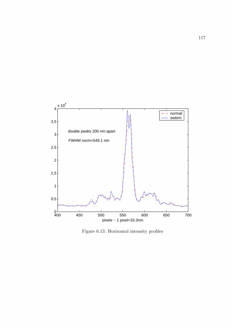
117
400 450 500 550 600 650 7000
0.5
1
1.5
2
2.5
3
3.5
4x 10
4
pixels − 1 pixel=33.3nm
normalswtirm
double peaks 200 nm apart
FWHM norm=549.1 nm
Figure 6.13: Horizontal intensity profiles

118
Figure 6.14: Chime model of β-carotene. H atoms are yellow, C atoms are cyan
however physical contraints proved too difficult to overcome to allow the successful
enhancement of Raman images by this method. Past experiments on the use of
total internal reflection geometries for Raman spectroscopy58 have had some suc-
cess in the study of surface chemistry with this method. Imaging is a more difficult
challenge because the bandpass filters used must be tuned correctly to the desired
Raman wavelength and have a limited throughput, decreasing the intensity of light
reaching the CCD camera. Due to the bandwidth (1 nm) of the filters used here,
a small error in the selected wavelength has a drastic effect on the transmitted in-
tensity. Spectroscopy experiments will typically use a monochromator and a highly
sensitive photomultiplier tube or intensified CCD which reduce the requirement for
high scattered light intensity.
The initial sample studied was β−carotene, selected for its resonance Raman
spectrum when illuminated with visible light. The resonance effect can increase the
Raman signal by 103−104×51. Figure (6.14) is a Chime model of β−carotene illus-
trating the eight isoprene units that make up the molecule. The long conjugated
chain is responsible for the orange color of the molecule. The samples were pre-
pared by dissolving β−carotene in methanol at about half the maximum solubility,

119
pipetting 100 µm onto a slide, and then letting the alcohol evaporate. The result
is a slide coated with small (≈ 10− 100) µm chunks of β−carotene scattered fairly
uniformly about the slide. The procedure for obtaining a Raman image was to tune
the bandpass filter to the appropriate wavelength for the desired Raman scattered
wavelength. The peak band is at 1516 cm−1 [59], which corresponds to a wave-
length of 572.8 nm. After exposing the CCD camera, the filter was retuned off-peak
to about 565 nm and 580 nm in order to acquire the fluorescence background for
subtraction in order to isolate the Raman signal. In practice, only one background
image was needed to provide satisfactory results.
The initial images shown in figure (6.15) show the white light image of a chunk of
β−carotene, along with a background fluorescence image (the image at the Raman
wavelength looks identical to the eye), and the Raman image after the fluorescence
background is subtracted. White light illumination does show the orange color of
the β−carotene, but this is lost on the monochrome CCD camera. This particular
sequence of images were acquired with the CCD camera set for 8x8 pixel binning for
higher sensitivity. The exposure time is 30 seconds and the laser power is 30%. The
scale bar in the white light is 100 µm. The second pair of images in figure (6.16) is
the result of an exposure at 30% laser power for 3 minutes without any pixel binning.
The white light image shows that the slide contains a lot of dust in addition to the
piece of β−carotene resolved by the Raman image. The β−carotene was confirmed
through the eyepiece by its organge color. The slide was inadvertanly dropped
before being mounted on the microscope, which resulted in the dust contamination.
This is an excellent example of the ability of Raman microscopy to discern different
molecular species. The next challenge was to obtain an SWTIRM image of the
Raman scattered light using the β−carotene sample. This was unsuccessful for two
principle reasons. The first was that it was difficult to make a sample with very
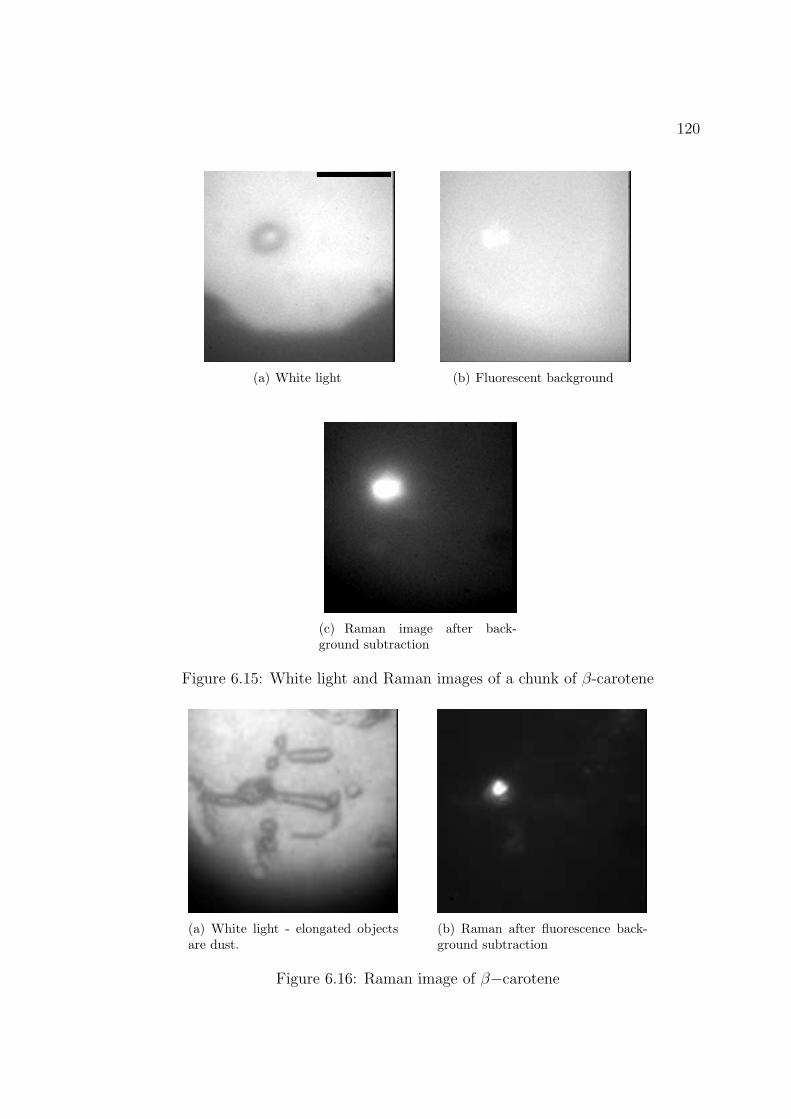
120
(a) White light (b) Fluorescent background
(c) Raman image after back-ground subtraction
Figure 6.15: White light and Raman images of a chunk of β-carotene
(a) White light - elongated objectsare dust.
(b) Raman after fluorescence back-ground subtraction
Figure 6.16: Raman image of β−carotene

121
small pieces (< 300 nm in diameter) of β−carotene which could be used to measure
a point spread function. The β−carotene has a very strong tendency to clump
as it dries in to micron sized chunks. Additionally, if the laser power or exposure
time was too high for better image contrast the β−carotene could be damaged, a
problem which was exacerbated with smaller pieces. This prevented effective use of
the photobleaching technique in which the sample is illuminated for sufficient time
to dampen out the fluorescence signal for somet time. The TIR illumination is only
effective with a penetration depth of a wavelength or so. In a micron-sized chunk,
the Raman scattered light emitted from this region then propagates and undergoes
Rayleigh scattering in the rest of the sample before reaching the objective located
on the far side of the sample from the illuminating light. One cure for this is to
attach the scattering molecule to a microsphere. Several consultations with Bangs
Laboratories and Polysciences, Inc. did not result in a method to do this because the
β−carotene does not readily form covalent bonds to carboxylate groups and other
commonly used molecules used to coat microspheres. The SWTIRM technique
relies on variations in intensity on length scales smaller than the laser wavelength,
and this additional scattering resulted in the subtle intensity variations being lost.
β−carotene is an effective sample for Raman imaging due to its resonance Raman
scattering, but it was not possible to obtain an SWTIRM image of this sample.
The second sample used for Raman imaging were 109 nm unlabeled polystyrene
microspheres. Figure (6.17) shows the reference Raman spectrum of polystyrene
published by the research group of Richard McCreery at Ohio State University c.
The peak intensity at 1001.4 cm−1 was selected for imaging, which corresponds to
a wavelength of 556.4 nm when using the 527 nm laser. The procedure was the
same as with the β−carotene, so the bandpass filter was tuned to 556.4 nm for
cWeb site: http://www.chemistry.ohio-state.edu/ rmccreer/freqcorr/images/poly.html

122
Figure 6.17: Reference Raman spectrum of polystyrene
the bandpass image, and then tuned down by 20 nm for the fluorescence image.
The Raman signal from the plain polystyrene was very weak, and the images in
figure (6.18) are the result of 10 minute exposures at 50% laser power. The Raman
image here does correspond to the bead positions. The weak Raman signal of the
polystyrene resulted in a new set of problems with obtaining a successful SWTIRM
image. The long exposure time exposed a slow drift in the micrometer that set the
instrument focus, which resulted in the slightly fuzzy final image. The high laser
power was also sufficient to burn a hole through the polarizer, but lowering the laser
power meant longer exposure times. The retroreflecting mirror is also mounted
on an open-loop piezo for translation, and there appears to be a combination of
thermal drift and piezo creep that resulted that caused additional trouble with the
collection of the intermediate images for SWTIRM. This was verified by attempting
to acquire SWTIRM images of fluorescent beads with 10 min intervals between image

123
(a) Bandpass image (b) Fluorescent background
(c) Raman image after background sub-traction
Figure 6.18: Raman image of 109 nm polystyrene microspheres. Scale bar is 10 µm

124
acquisitions. The use of the microstepping motor to hold the tunable bandpass filter
may have contributed a degree of vibration to the system despite the rigidity of the
microscope structure. Microstepping motors exert a holding torque and have a very
small mechanical wiggle when they are set to a fixed position. The fluorescence
background could be eliminated by the use of a near-infrared laser, but there is a
corresponding loss of resolution due to the longer wavelength λ, as well as a decrease
in the amount of signal since the scattering is proportional to the wavelength as λ−4.
There are several other methods of exciting Raman scattering that may over-
come the problems associated here with enhancing the resolution by the SWTIR
technique. Among these are stimulated Raman12, surface-enhanced Raman13 14,
and coherent anti-Stokes Raman (CARS)15. The primary problems are the subtrac-
tion of the fluorescence background and long CCD integration times. CARS uses a
pump-probe method to selectively enhance the anti-Stokes Raman scattering from
a molecule. Since the anti-Stokes scattering is higher in energy, there is no fluores-
cence background at all. The basic idea of the technique is to use a pump beam at
frequency ωp and a Stokes laser beam at frequency ωS. These combine in a four-wave
mixing process to generate an anti-Stokes signal at frequency ωAS = 2ωp − ωS12.
This has been used successfully in microscopes built for biological samples60. In
stimulated Raman, two laser beams are used, a fixed pump beam at frequency ωp
and a tunable probe beam at frequency ωS where ωS < ωp. Figure (6.19(b)) illus-
trates the energy diagram. If the probe beam is tuned to a Stokes mode, then each
pump photon has a high probability of conversion to a Stokes scattered photon. In
practice, conversion rates of higher then 50% are possible61.
Surface enhanced Raman scattering (SERS) has the highest potential for increas-
ing the Raman signal from a sample, with enhancements as high as 1014 having been
observed62, also 106 is the more typical level achieved. This enhancement is observed

125
ground state
Raman vibrationalstate
ωp ω
S
ωp
ωAS
Virtual state 2
Virtual state 1
(a) Energy diagram for CARS
ground state
Raman vibrationalstate
ωp ω
S
Virtual state
(b) Energy diagram for stimulated Raman
when the scattering molecule is adsorbed on or within a few nanometers of a struc-
tured metal surface. The effect is highest for silver but can also be accomplished
with gold or copper. There is one principal mechanism by which the enhanced
Raman signal is generated63. This involves the formation of surface plasmon res-
onances in the metal surface formed when conduction electrons are excited by the
laser wavelength. An exceptionally large electric field is generated which then causes
the Raman scatter from the adsorbed molecule. These enhanced Raman technique
have the potential to solve the various difficulties that were unable to be overcome
in the application of SWTIR to the Raman effect. The potential new problems will
most likely involve the formation of the correct evanescent field with the multiple
laser beams involved. In the case of SERS, the metal substrate or metal particles
will have an interaction with the evanescent field which will have to be carefully
studied.

126
6.8 Conclusions
The standing wave total internal reflection technique is an effective means of in-
creasing the resolution of an optical microscope using an interference pattern in
the evanescent field and a Fourier decomposition algorithm. The limited penetra-
tion depth of the evanescent field limits this technique to thin samples, such as cell
membranes or spin-coated proteins. Imaging fluorescent samples is straightforward
once the microscope is in working order, and resolution as high as 170 nm has been
achieved with a 1.33 NA objective and a laser with a wavelength of 527 nm, an
improvement of 280%. The extension of the SWTIR technique to Raman imaging
was unsuccessful, due to interference from the fluorescence background, thermal
and mechanical drift of the instrument during long exposures, and signal-to-noise
problems. Normal Raman imaging can be accomplished which is useful in the same
manner as fluorescence for imaging of thin samples.

Chapter 7
Lattice Gas Simulations of
Surfactant Systems
7.1 Introduction
We present simulation studies of temperature quenches in a two-dimensional lat-
tice gas model of microemulsions. A series of temperature quenches from above
the critical mixing temperature was done for several different concentrations of sur-
factant in an oil-water-surfactant mixture. Spontaneous micellization was observed
for several quench depths in all concentrations. A stretched-exponential curve was
found to fit the growth of the average structure size. The relaxation time of the
stretched-exponential follows a Vogel-Fulcher growth law for low temperatures.

128
7.2 Background and the Lattice-Gas Automata
Model
Oil and water do not mix, but with the addition of amphiphile (or surfactant)
chemicals to the system a wide range on complex structures can be observed. The
surfactant molecules are typically polar in nature, typically with an ionic head at-
tracted to water and a hydrocarbon tail attracted to oil. There is a strong energy
preference for the surfactant molecules to be absorbed on oil-water interfaces, which
leads to the formation of such interfaces. In this paper a lattice gas model is used
to model the dynamics of these oil-water-surfactant systems under temperature
quenching conditions. We use a lattice gas model for the nonequilibrium dynamics
of microemulsions that has been previously developed by Boghosian, Coveney, and
Emerton16. The model has been used to study domain growth, self-assembly64,
and shear-induced lamellar transitions65 in amphiphilic fluids. Other models for the
study of surfactant-oil-water systems include lattice Boltzmann methods66 in two
and three dimensions as well as a three dimensional version of the lattice gas model
used here67.
The lattice-gas model used is based on an immiscible lattice-gas model due to
Rothman and Keller68. It is extended to include dipolar surfactant molecules along-
side the oil and water particles. A triangular lattice is used with lattice vectors
ci(i = 1, . . . , 6), and the state of the 2D model at site x and time t is completely
specified by the occupation numbers nαi (x, t) ∈ 0, 1 for particles of species α and
velocity ci/∆t.
The time evolution of the lattice gas takes place in two steps, a streaming substep
followed by a collision substep. The streaming substep updates the lattice to move
the particles along their associated lattice vectors. The collision substep implements

129
a set of collision rules that change the state of the newly arrived particles in a way
that preserves the mass of each species as well as the total momentum.
The immiscible species (oil and water) are represented in the Rotham and Keller
lattice-gas as two different colors, α = B (blue) for water, and α = R (red) for oil.
A color charge is defined as qi(x, t) ≡ nRi (x, t) − nB
i (x, t) for a particle moving
in direction i at time t and position x. A color potential φ of a color charge is
then defined as φ = qf(r) at a distance r from the charge, where f(r) is some
specified function that defines the strength and type of the potential. The energy
of interaction between q and q′ is Hcc = q′φ(r) = qq′f(r). The collision substep
preserves the total momentum and mass of each species, so the only contribution to
the interaction energy will come during the streaming substep where the outgoing
color charges do work in moving to their new sites. The interaction energy involves
the outgoing particle q′i(x, t) at x ∈ L and the total color charge q(x + y, t) at site
x + y ∈ L. The total color work performed is finally defined as
∆Hcc(x, t) = J(x, t) · E(x, t)∆t.
J(x, t) is defined as the color flux, and E(x, t) is defined as the color field.
For a full description of the lattice gas model, please refer to the original publica-
tion by Boghosian, Coveney, and Emerton16. The model is extended to include sur-
factant by defining a third species S and an associated occupation number nSi (x, t)
to represent the presence or absence of a surfactant particle. Additionally, each
surfactant particle is modeled (analogously with electrostatics) as a red-blue dipole
σi(x, t) with a free orientation. This three-component model includes three addi-
tional interaction terms aside from φ: the color-dipole field, the dipole-color field,
and dipole-dipole interactions. The color-dipole field is defined as

130
-¢¢
−q
+qa
x yQ -¢
¢
AAU
−q1
+q1a1
x y−q2
+q2
a2
-AAU
Qx y
−q
+qa
Figure 7.1: The interaction models - (a) color-dipole, (b) dipole-color, and (c) dipole-dipole
Hcd = qQ[+f(|y + a|)− f(|y|)]
In the limit of a → 0 and q →∞, so that qa → σ, this becomes
Hcd = −f1(y)Qσ · y
Color charge is conserved by the dynamics, so the only local energy change that
needs to be incorporated into the Hamiltonian due to the color-dipole interaction
from the outgoing particles doing work in moving to their new sites. The interaction
energy between an outgoing particle with color charge q′i(x, t) at x ∈ L and the total
dipole vector σ(x + y) at site x + y ∈ L is given by
∆Hcd = J(x, t) ·P(x, t)∆t
where P(x, t) is a dipolar field vector. The next term that is required is the work
done by a color dipole σ moving in a field of fixed color charge Q, at a displacement
y, as shown in figure 7.1. The energy of the static interaction is

131
Hdc = qQ[+f(|y − a|)− f(|(y)|)]
In the limit that a → 0 and q →∞ so that qa → σ, this becomes
Hdc = +f1(|y|)Qσ · y.
The total dipolar color work is
∆Hdc(x, t) = σ′(x, t) · E(x, t) + Tr (J (x, t) · E(x, t)) ∆t
where σ′ is the total outgoing dipole vector, J (x, t) is the dipolar flux tensor, and
E(x, t) is the color field gradient tensor.
The last piece to consider is the dipole-dipole interaction. The static interaction
between a dipole sigma1 moving in the field of a fixed dipole σ2 at a distance y is:
Hdd = q1q2[−f(|y − a1|)− f(|y + a2|) + f(|y + a2 − a1|) + f(|y|).
In the limit as aj →∞ and qj → 0, so that qjaj → sigmaj, this becomes
Hdd = −f2(y)(σ1 · y)(σ2 · y) + f1(y)σ1 · σ2
Some further analysis, followed by summing over all outgoing color dipoles at site x
and over all sites y ∈ L with which they might interact gives the total interdipolar
color work, ∆Hdd:
∆Hdd(x, t) = σ′(x, t) ·P(x, t) + Tr(J (x, t) · P(x, t))∆t
J (x, t) is the dipolar flux tensor, and P(x, t) is the dipolar field gradient tensor.

132
Adding a set of coupling constants for the most general form of the interaction
energy gives:
∆Hint = α∆Hcc + µ∆Hcd + ε∆Hdc + ζ∆Hdd
Outgoing states are then sampled with probability:
P ∝ e−β∆Hint
where β acts as an inverse temperature-like parameter. The average size of the
structures (< R(t) >) is calculated by numerically evaluating the circularly averaged
structure factor.16
There are previous experimental and numerical results that suggest the rate
of growth of the average size of structure in a micellar are reasonably fitted to a
stretched-exponential function69. This function has the form:
〈R〉(t) = R∞ − (R∞ −R0)e(− t
τ)γ
(7.1)
The quantities R∞, R0, τ , and γ are free parameters.
7.3 Experiment Details
In this paper we will describe the results of a large set of simulations using this
model to study the effects of temperature quenching on the system dynamics. A
128x128 lattice size was used for all the simulations in these results. Following the
parameters used in earlier studies, the values of the coupling constants were chosen
as:
α = 1.0 µ = 0.05 ε = 8.0 ζ = 0.5
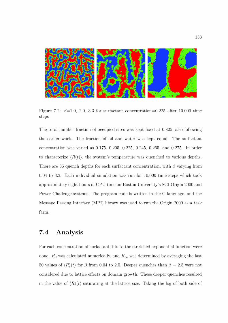
133
Figure 7.2: β=1.0, 2.0, 3.3 for surfactant concentration=0.225 after 10,000 timesteps
The total number fraction of occupied sites was kept fixed at 0.825, also following
the earlier work. The fraction of oil and water was kept equal. The surfactant
concentration was varied as 0.175, 0.205, 0.225, 0.245, 0.265, and 0.275. In order
to characterize 〈R(t)〉, the system’s temperature was quenched to various depths.
There are 36 quench depths for each surfactant concentration, with β varying from
0.04 to 3.3. Each individual simulation was run for 10,000 time steps which took
approximately eight hours of CPU time on Boston University’s SGI Origin 2000 and
Power Challenge systems. The program code is written in the C language, and the
Message Passing Interface (MPI) library was used to run the Origin 2000 as a task
farm.
7.4 Analysis
For each concentration of surfactant, fits to the stretched exponential function were
done. R0 was calculated numerically, and R∞ was determined by averaging the last
50 values of 〈R〉(t) for β from 0.04 to 2.5. Deeper quenches than β = 2.5 were not
considered due to lattice effects on domain growth. These deeper quenches resulted
in the value of 〈R〉(t) saturating at the lattice size. Taking the log of both side of

134
0 1 2 3 4 5 6 7 8 9 10−10
−8
−6
−4
−2
0
2
4surfactant concentration 24.5%
log(t)
f(<
R>
(t))
Figure 7.3: The stretched exponential fit, surfactant concentration 0.245
equation 7.1 twice yields:
g(t) = log(− log
(R∞ − 〈R〉R∞ −R0
))= γ log(t/τ)
From these fits, values for the constant γ and the relaxation time τ are calculated.
As seen in figure 7.4, γ generally decreases with increasing surfactant concentration.
Figure 7.5 plots the value of τ versus temperature for all surfactant concentrations.
The low-temperature behavior suggests a Vogel-Fulcher type growth law, of the
form:
τ = exp
(B(ns)
T − T∞(ns)
)
B(ns) is a parameter dependent on the surfactant concentration, and T∞ is the
temperature below which the relaxation time is infinite. The higher temperature
behavior of τ is evidently not following a Vogel-Fulcher growth law. There may be a
functional form of τ = f(T )V (T ) where V (T ) is the Vogel-Fulcher law and f(T ) is
some modifying function of the temperature. Figure 7.6 plots log(τ) vs. (T−T∞) for

135
0.2 0.25 0.30.5
0.55
0.6
0.65
0.7
0.75
0.8
0.85
0.9
γ
Figure 7.4: γ vs. surfactant concentration
0 5 10 15 20 250
500
1000
1500
2000
2500
3000
3500
4000
4500
5000
τ
17.5%20.5%22.5%24.5%26.5%27.5%
Figure 7.5: τ vs. temperature

136
−2.5 −2 −1.5 −1 −0.5 0 0.50.1
0.12
0.14
0.16
0.18
0.2
0.22
1/log(τ) vs. (T−Tinf
)
T−Tinf
1/lo
g(τ)
17.5%20.5%22.5%24.5%26.5%27.5%
Figure 7.6: 1ln(τ)
vs. (T − T∞)
all surfactant concentrations. Vogel-Fulcher growth dynamics have been observed
in simulations of physically associating polymer solutions70 and in the dynamics
of isotropic-nematic phase transitions in silica gels71, along with numerous glassy
systems.
An example of spontaneous micelle formation can be seen in the middle image of
figure 7.2. This occurred for all surfactant concentrations with temperature quenches
in the range of β = 1.8 to 2.3. A simulation run of 100,000 time steps was done
for β = 2.0 and a surfactant concentration of 22.5%. The micelles were stable
upon a phase-separating background of oil and water. Animations of the simulation
show that the micelles form once the oil and water have largely phase-separated
with a surfactant layer in between. The micelles form along the surfactant-oil and
surfactant-water boundaries. In order to further investigate this behavior, the last
time step of each simulation run had the thickness of its surfactant layer measured.
In order to calculate the layer thickness, a set of lines is used as a mask with the
surfactant layer. The resulting line segments then have their lengths calculated, and

137
0.5 1 1.5 2 2.5 3
2
3
4
5
6
7
8
β
pix
el w
idth
0.2750.2650.2450.2050.175
Figure 7.7: Surfactant layer thickness
2/3 the average segment length yields the layer thickness72. The layer thickness in
pixels for each surfactant concentration is plotted versus β in figure (7.7) with the
micelle growth region delineated by dashed horizontal lines. Close examination of
the animations of the simulations indicate that the micelles form at more heavily
curved sections of the surfactant layer the fluctuations in the layer. Quenches that
are too shallow to form micelles do not have a thick enough surfactant layer, and
conversely quenches that are too deep form a surfactant layer that is too thick.
The deepest quenches eventually phase separate completely if they are run far past
10,000 time steps. What is not evident from this plot is that for the higher values
of β the surfactant layer thickness certainly includes the range of critical values but
does not remain there since it continually thickens as the simulation runs.

138
7.5 Conclusions
The stretched exponential function is a reasonable fit to the growth dynamics of
lattice-gas simulations of amphiphilic fluids. Stretched exponential behavior is a
recurrent theme in this thesis and it is observed when the dynamics of a system are
constrained in some fashion to prevent the system from accessing all points in its
phase space. Here the constraint is due to the interactions between the particles
interacting on the lattice. The relaxation time follows a Vogel-Fulcher growth law
for low temperatures. Vogel-Fulcher behavior is typically observed near the temper-
ature for a phase transition. Micelles were observed to form at regions with high
curvature provided the layer thickness is within a certain range for a long enough
time. These micelles are stable against the phase separating background of oil,
water, and surfactant.

Chapter 8
Discussions and Conclusions
8.1 The Dynamic Light Scattering Microscope
The design and construction of a DLS microscope achieved its goals. The instru-
ment has a small scattering volume of approximately 10 nL, a selectable scattering
volume using the microscope optics, and a well-defined scattering angle. This in-
strument improves upon the initial design by Prof. David Weitz’s group at Harvard
in its calibration and its ease of use. The small scattering volume allows for the
observation of nonergodic dynamics in appropriate samples and additionally rhe-
ological parameters can be measured using microspheres as tracer particles. The
DLS microscope has proven effective for studying polymers and gels for biological
applications.
8.1.1 Porcine Gastric Mucin
The porcine gastric mucin (PGM) glycoprotein is a large molecule that is the prin-
cipal component of the mucus layer lining the stomach in pigs. In general, the
viscoelastic properties of mucin allow for the lubricative and protective properties

140
of the mucus layer. The PGM was studied at pH 2 and pH 6 both by scattering from
the pure mucin and by scattering from embedded 109 nm polystyrene microspheres.
At pH 6 the mucin is in a semidilute polymer solution, and the pure solution did not
provide enough scattering for measurement with the DLS microscope. The addition
of the polystyrene microspheres allowed for the measurement of stretched exponen-
tial behavior in the bead dynamics with the stretching exponent β = 0.7pm0.05.
The microspheres experience a viscosity twice that of water in the semidilute poly-
mer solution. At pH 2 the mucin forms a gel, and scattering from the pure gel shows
dynamics that follow a power law with an exponent α = 0.26 and an amplitude of
only 0.07, along with a dominating stretched exponential with the stretching expo-
nent β = 0.98. The autocorrelation function from scattering off of the polystyrene
microspheres displays nonergodic dynamics. The theoretical method by Pusey, et.
al. allows for the analysis this data to dertermine the microviscosity experienced by
the beads. This microviscosity is 1.3× greater than water.
8.1.2 Matrigel
Matrigel is a commercial basement membrane which was also studied with the light
scattering microscope. Again, the pure gel, after preparation following the manufac-
turer’s instructions, showed stretched exponential behavior with β = 0.14. The 109
nm microspheres in Matrigel experience a microviscosity identical to that of water
at room temperature, indicating that the components that make up the gel are not
interacting with the beads in a significant manner. 510 nm beads were also added
to the Matrigel and their dynamics were analyzed in terms of their mean square
displacement to yield an estimate of the low-frequency elastic shear modulus with
a value of 50.2± 6.0 dynes/cm2.

141
8.2 The Standing Wave Total Internal Reflection
Microscope
The standing wave total internal reflection technique is an effective means of in-
creasing the resolution of an optical microscope using an interference pattern in
the evanescent field and a Fourier decomposition algorithm. The limited penetra-
tion depth of the evanescent field limits this technique to thin samples, such as cell
membranes or spin-coated proteins. Imaging fluorescent samples is straightforward
once the microscope is in working order, and resolution as high as 170 nm has been
achieved with a 1.33 NA objective and a laser with a wavelength of 527 nm, an
improvement of 280%. The extension of the SWTIR technique to Raman imaging
was unsuccessful, due to interference from the fluorescence background, thermal and
mechanical drift of the instrument during long exposures, and signal-to-noise prob-
lems. Normal Raman imaging was successfully demonstrated which is useful in the
same manner as fluorescence for imaging of thin samples.
8.3 Lattice Gas Simulations of Surfactant Sys-
tems
This section described the results of a set of simulations of oil–water–surfactant
systems in two dimensions. This set of simulations was conducted in two dimensions
using a lattice gas model of microemulsions. The dynamics of the system show
stretched exponential growth for the average structure size in the system and the
relaxation times of these stretched exponential fits follow a Vogel-Fulcher growth
law. Micelles were observed to form at regions with high curvature provided the
layer thickness is within a certain range for a long enough time. These micelles are

142
stable against the phase separating background of oil, water, and surfactant.
8.4 Future Work
Both optical instruments are the subject of further development. The DLS micro-
scope is being upgraded with a second photomultiplier tube and a beamsplitting
fiber. In this arrangement, where the detected scattered light is split into two fibers
and sent to two PMTs, the signal is cross-correlated between the two detectors rather
than autocorrelated. The result is that the afterpulsing of the PMTs is not corre-
lated and there is an improvement in data collection at very short time scales. The
dynamics of PGM will be further studied using larger bead sizes and at additional
pH levels. A suggested experiment is a measurement of the dynamical properties
of pH 2 mucin after the addition of the h. pylori bacterium. A second experiment
should involve the addition of droplets of acid to a mucin sample at high pH to
mimic the introduction of acid into the stomach through the mucus layer. These
experiments exploit the spatial selectivity of the DLS microscope and provide physi-
ological models for study. Matrigel will be further characterized using bead tracking
microrheology and electron microscopy. The DLS microscope can also be used in
a diffusive wave spectroscopy mode, and future experiments should be arranged to
test this mode of operation.
The fluorescent SWTIR microscope is in active development by a graduate stu-
dent at the Massachusetts Institute of Technology in the laboratory of Peter So.
Raman imaging using the SWTIR technique is in principle still possible, and tech-
niques that enhance the Raman signal such as coherent anti-Stokes Raman are the
most promising route to enhancing Raman imaging past the diffraction limit.

Appendix A
The Stokes-Einstein Relation
Brownian motion is the random walk motion of small particles suspended in a fluid.
The random motion, discovered by biologist Robert Brown in 182873, is due to
bombardment of the particles by the fluid molecules obeying a Maxwellian velocity
distribution. Albert Einstein74, in one of his early theoretical accomplishments, used
kinetic theory to derive the diffusion constant for such motion in terms of funda-
mental parameters of both the particles and the fluid. The derivation of Brownian
motion begins with the Langevin equation, which adds a random noise term to
equation of motion for a free particle of mass M :
MdV
dt= −ζV + F(t) (A.1)
where ζ is the friction constant and F(t) is a random force. For a sphere of radius
r, the friction constant comes from the Stokes drag formula which gives for stick-
boundary conditions ζ = 6πηr where η is the viscosity of the fluid. On average
there will be more collisions on the front of the particle than the back due to the
particle’s motion which gives rise to the friction term. The random force is due to
the collisions with the molecules that make up the fluid which are sufficient to keep

144
the particle in perpetual thermal motion.
In order to solve the Langevin equation, the statistical properties of F(t) must
be described. The Maxwell velocity distribution for a molecule of mass m is:
N(r, v)d3rd3v =N
V
(m
2πkBT
)3/2
e−mv2/2kBT d3rd3v (A.2)
For an individual velocity component the distribution is:
N(vx)dvx =
∫ ∞
−∞
∫ ∞
−∞N(vx, vy, vz)dvydvz
=N
V
(√2πkBT
m
)2 (m
2πkBT
)3/2
e−mv2x/2kBT dvx
=N
V
(m
2πkBT
)1/2
e−mv2x/2kBT dvx (A.3)
The distribution of speeds is:
N(v)dv = 4πv2N(v)d3v
= 4πN
V
(m
2πkBT
)3/2
v2e−mv2/2kBT dv. (A.4)
Here, N is the number of particles, V is the system volume, kB is the Boltzmann
constant, and m the particle mass.
The general solution of the Langevin equation is
V(t) = V(0)e−( ζM )t +
∫ t
0
e−( ζM )(t−τ)F(τ)dτ. (A.5)
The velocity correlation function can be determined here by taking the dot product
of V(0) with each term and the averaging over the specified Maxwell distribution

145
of velocities. This gives
〈V(0) ·V(t)〉 = 〈V(0) ·V(0)〉e−( ζM )t +
∫ t
0
e−( ζM )(t−τ)〈V(0) · F(τ)dτ〉. (A.6)
Since the random force is assumed to be uncorrelated with the initial velocity due
to its origin in thermal fluctuations in the fluid, the second term in equation (A.6)
is 0. The velocity correlation function ψ(t) for a Brownian particle is therefore
ψ(t) ≡ 〈V(0) ·V(t)〉 =3kBT
Me−( ζ
M )t (A.7)
where the equipartition theorem has been applied:
1
2M〈V(0) ·V(0)〉 =
1
2M〈V 2〉 =
3
2kBT. (A.8)
Studying the velocity correlation function of the Gaussian random motion of the
particle yields an association between the diffusion constant and the time-integral
of the particle velocity correlation function:
D =1
3
∫ ∞
0
dτ〈V(0) ·V(t)〉 (A.9)
Substitution of ψ(t) into equation (A.9) gives the Stokes-Einstein relation:
D =kBT
ζ=
kBT
6πηr. (A.10)

Appendix B
Diffusing Wave Spectroscopy
Diffusing wave spectroscopy (DWS) is a relatively recent75 technique that deals
with multiply-scattered photons from a sample, whereas DLS is restricted to single-
scattered photons. In DWS, the transport of light through the sample is modeled as
a diffusion process, where the electric field autocorrelation function being expressed
as76:
G(1)(τ) ∝∫ ∞
0
P (s)e−(2τ/τ0s/l∗)ds (B.1)
Here, τ is the delay time, P (s) is the probability that the light travels a path of
length s, τ0 = 1/Dk20, k0 = 2π/λ, and l∗ is the mean free path. This equation
means that a photon traveling a path s has moved s/l∗ mean free paths and that
G(1) decays on average by a factor of exp(−2τ/τ0) per step. The most rapid decays
are therefore due to the longest paths. The determination of P (s) is entirely due
to the geometry of the experimental system. For a plane wave in the z direction
incident on a ’slab’ sample of thickness L, P (s) is proportional to the time depence
of the light intensity emerging from the sample:
P (s) ∝ z · ∇Iout(x, y, z, t) (B.2)

147
If the wave function U is solved in the diffusion equation ∂U/∂t = D∇2U , the
observation that G(1)τ is the Laplace transform of P (s) gives for the form of G(1) 75:
G(1)(τ) =L
γl∗sinh [γ(6τ/τ0)
1/2]
sinh [(L/l∗)(6τ/τ0)1/2]
≈ L
l∗(6τ/τ0)
1/2
sinh [(L/l∗)(6τ/τ0)1/2](B.3)
The factor γ is the number of mean free paths the photon travels before scattering.
If the time scale τ is much less than the relaxation time then the second equation
(B.3) holds. A fit to the measured G(2)(τ) gives the mean free path l∗.
The DLS microscope can be adopted to perform DWS measurements by moving
the collection fiber onto the optical axis of the microscope and the direct laser beam.
Angular information is lost due to the multiple scatters. The sample would have
to scatter very strongly, be quite thick, or both in order to ensure that multiple
scattering events are occuring. An additional step to avoid nonergodic effects can
be taken77, which involves placing a second scattering sample after the first which
provides averaging of the signal from the first sample. In this “two-cell” method
the second sample is typically polystyrene microspheres in glycerol which has very
slow dynamics. Since the time scale resolution of DWS is very high, the additional
scattering should only serve to average to desired signal and not alter the high-speed
dynamical behavior that is of interest. It is an open question as to whether the DLS
microscope with its very small scattering volume can be adopted to perform DWS
measurements in this manner.

Bibliography
1. Joyce Anne Peetermans. Brownian Motion of Macromolecules Inside Single
Intact Biological Cells: Microscope Laser Light Scattering Spectroscopy. Ph.d.,
Massachuetts Institute of Technology, September 1985.
2. P.D. Kaplan and D.A. Weitz, A Light Scattering Microscope, Applied Optics
38, 4151–5157 (1999)
3. Xingxiang Cao, Rama Bansil, K. Ramakrishnan Bhaskar, Bradley S. Turner,
J. Thomas LaMont, Niu Niu and Nezam H. Afdhal, pH-Dependent Conforma-
tional Change of Gastric Mucin Leads to Sol-Gel Transition, Biophysical Journal
76, 1250–1258 (March 1999)
4. Mark E. Keegan, Judith A. Whittum-Hudson and W. Mark Saltzman,
Biomimetic design in microparticulate vaccines, Biomaterials 24, 4435–4443
(2003)
5. Lisa A. Flanagan, Yo-El Ju, Beatrice Marg, Miriam Osterfield and Paul A. Jan-
mey, Neurite branching on deformable substrates, Developmental Neuroscience
13(18), 2411–2415 (December 2002)
6. Mats Gustafsson, D.A. Agard and J.W. Sedat, I5M: 3D widefield light mi-
148

149
croscopy with better than 100 nm axial resolution., Journal of Microscopy 195,
6–10 (July 1999)
7. J.T. Frohn, H.F. Knapp and A. Stemmer, True optical resolution beyond the
Rayleigh limit achieved by standing wave illumination,, Proceedings of the Na-
tional Academy of Sciences 97(13), 7232–7236 (2000)
8. Stephen W. Hell and J. Wichmann, Breaking the diffraction resolution limit by
stimulated emission: stimulated-emission depletion microscopy, Optics Letters
19, 780–782 (1994)
9. Marcus Dyba, Stefan Jakobs and Stefan W. Hell, Immunofluorescence stimu-
lated emission depletion microscopy, Nature Biotechnology 21(11), 1303–1304
(November 2003)
10. S.M. Mansfield and G.S. Kino, Solid immersion microscope, Applied Physics
Letters 57, 2615–2616 (1990)
11. Peter T. C. So, Hyuk-Sang Kwon and Chen Y. Dong, Resolution Enhancement
in standing-wave total internal reflection microscopy: a point-spread-function
engineering approach, Journal of the Optical Society of America A 18(11), 2833–
2845 (2001)
12. Derek A. Long, The Raman Effect, John Wiley and Sons, Ltd., New York, 2002
13. Joel I. Gersten, Ronald L. Birke and John R. Lombardi, Theory of Enhanceed
Light Scattering from Molecules Adsorbed at the Metal-Solution Interface,
Physics Review Letters 43(2), 147–150 (1979)
14. R. Varma and J.R. Selman, Herausgeber. Techniques for Characterization of

150
Electrodes and Electrochemical Processes, Kapitel Surface Enhanced Raman
Spectroscopy. Wiley-Interscience, New York, 1991. author R. Birke.
15. Sylvie A. J. Druet and Jean-Pierre E. Taran, Cars spectroscopy, Progress in
Quantum Electronics 7, 1–72 (1981)
16. B.M. Boghosian, P.V. Coveney and A.N. Emerton, A Lattice-Gas Model of
Microemulsions, Proceedings of the Royal Society of London 452, 1221–1250
(1996)
17. Eugene Hecht, Optics: Second Edition, Addison-Wesley, Reading, 1987
18. Max Born and Emil Wolf, Principles of Optics, Cambridge University Press,
Cambridge, 1999
19. S. G. Lipson, H. Lipson and D. S. Tannhauser, Optical Physics: Third Edition,
Cambridge University Press, Cambridge, 1995
20. Eugene Butkov, Mathematical Physics, Pearson Education POD, 1968
21. D.A. Weitz, J. X. Zhu, D.J. Durian, H. Gang and D.J. Pine, Diffusing wave
spectroscopy: the technique and some applications, Physica Scripta T49, 610–
621 (1993)
22. Benjamin Chu, Laser Light Scattering, Academic Press, New York, 1991
23. John David Jackson, Classical Electrodynamics: 3rd Edition, John Wiley and
Sons, New York, 1998
24. Robert Pecora, Herausgeber, Dynamic Light Scattering: Applications of Photon
Correlation Spectroscopy, Plenum Press, New York, 1985

151
25. Stephen W. Provencher, CONTIN: A general purpose constrained regularization
program for inverting noisy linear algebraic and integral equations., Computa-
tional Physics Communications 27, 219 (1982)
26. Jaromir Jakes, Regularized positive exponential sum (REPES) program - a
way of inverting Laplace transform data obtained by dynamic light scattering,
Collection of Czechoslovakian Chemical Communications 60, 1781–1797 (1995)
27. P.N. Pusey and W. van Meegan, Dynamic light scattering by non-ergodic media,
Physica A 157, 705 (1989)
28. Jacques G.H. Joosten, Erik T.F. Gelade and Peter N. Pusey, Dynamic light
scattering by nonergodic media: Brownian particles trapped in polyacrylamide
gels, Physical Review A 42(4), 2161–2175 (1990)
29. Isabel Behrens, Ana Isabel Vila Pena, Maria Jose Alonso and Thomas Kissel,
Comparative Uptake Studies of Bioadhesive and Non-Bioadhesive Nanoparticles
in Human Intestinal Cell Lines and Rats: The Effect of Mucus on Particle
Adsorption and Transport, Pharmaceutical Research 19(8), 1185–1193 (August
2002)
30. Joel Keizer, Statistical Thermodynamics of Nonequilibrium Processes, Springer-
Verlag, New York, 1987
31. T.G. Mason, Hu Gang and D.A. Weitz, Diffusing-wave-spectroscopy measure-
ments of viscoelasticity of complex fluids, Journal of the Optical Society of
America A 14(1), 139–149 (1997)
32. T.G. Mason and D.A. Weitz, Optical measurements of the frequency-dependent
linear viscoelastic moduli of complex fluids., Physical Review Letters 74, 1250–
1253 (1995)

152
33. Z. Hong, B. Chasan, R. Bansil, B. Turner, K.R. Bhaskar and N.H. Afdhal.
Atomic force microscopy of gastric mucin. poster presentation, 2001.
34. K.L. Ngai and George D.J. Phillies, Coupling model analysis of polymer dy-
namics in solution: Probe diffusion and viscosity, Journal of Chemical Physics
105(18), 8385–8397 (November 1996)
35. Bo Nystrom, Harald Walderhaug and Finn Knut Hansen, Dynamic Crossover
Effects Observed in Solutions of a Hydrophobically Associating Water-Soluble
Polymer, Journal of Physical Chemistry 97, 7743–7752 (1993)
36. C.Konak, M.Konak and R. Bansil, Dynamic Light Scattering of Particles Dif-
fusing Within a Microscopic Cage: Model Calculations, Physica A 171, 19–25
(1991)
37. M.T. Valentine, P.D. Kaplan, D. Thota, J.C. Crocker, T. Gisler, R.K.
Prud’homme, M. Beck and D.A. Weitz, Investigating the microenvironments
of inhomogeneous soft materials with multiple particle tracking, Physical Re-
view E 64, 061506–1 – 061506–9 (2001)
38. Frank Sheffold, Particle Sizing with Diffusing Wave Spectroscopy, Journal of
Dispersion Science and Technology 23(5), 591–599 (2002)
39. Stuart S. Olmsted, Janet L. Padget, Ashley I. Yudin, Kevin J. Whaley,
Thomas R. Moench and Richard A. Cone, Diffusion of Macromolecules and
Virus-Like Particles in Human Cervical Mucus, Biophysical Journal 81, 1930–
1937 (October 2001)
40. Lei Shi and Karin D. Caldwell, Mucin Adsorption to Hydrophobic Surfaces,
Journal of Colloid and Interfacial Science 224, 372–381 (2000)

153
41. Hynda K. Kleinman, Mary L. McGarvey, John R. Russell, Vicki L. Star,
Frances B. Cannon, Gordon W. Laurie and George R. Martin, Basement Mem-
brane Complexes with Biological Activity, Biochemistry 25, 312–318 (1986)
42. S. Vukicevic, H.K. Kleinman, F.P. Luyten, A.B. Roberts, N.S. Roche and A.H.
Reddi, Identification of multiple active growth factors in basement membrane
Matrigel suggests caution in interpretation of cellular activity related to extracel-
lular matrix components., Experimental Cell Research 202(1), 1–8 (September
1992)
43. A.R. Mackay, D.E. Gomez, D.W. Cottam, R.C. Rees, A.M. Nason and
U.P. Thorgeirsson, Identification of the 72-kDa (MMP-2) and 92-kDa (MMP-
9) gelatinase/type IV collagenase in preparations of laminin and Matrigel.,
BioTechniques 15, 1048 (1993)
44. P.G. McGuire and N.W. Seeds, The interaction of plasminogen activator with
a reconstituted basement membrane matrix and extracellular macromolecules
produced by cultured epithelial cells., Journal of Cell Biochemistry 40(2), 215–
227 (1989)
45. A.P. Balgude, X. Yu, A. Szymanksi and R.V. Bellamkonda, Agarose gel stiffness
determines rate of DRG neurite extension in 3D cultures, Biomaterials 22, 1077–
1084 (2000)
46. American Society of Mechanical Engineers. Effect of Substrate Stiffness on Cell
Morphology, Bioengineering Conference. ASME Technical Publishing, 2001.
47. T.G. Mason, K Ganesan, J.H. van Zanten, D. Wirta and S.C. Kuo, Particle
Tracking Microrheology of Complex Fluids, Physical Review Letters 79(17),
3282–3285 (October 1997)

154
48. D. Stamenovic and M.F. Coughlin, The role of prestress and architecture of
the cytoskeleton and deformability of cytoskeletal filaments in mechanics of
adherent cells: a quantitative analysis, Journal of Theoretical Biology 201(1),
63–74 (1999)
49. C. V. Raman and K. S. Krishnan, A New Type of Secondary Radiation, Nature
121(501), 3048 (March 1928)
50. J.J. Sakurai, Modern Quantum Mechanics, Addison-Wesley, revised edition edi-
tion, 1994
51. John R. Ferraro, Kazuo Nakamoto and Chris W. Brown, Introductory Raman
Spectroscopy, Academic Press, San Diego, 2nd edition, 2003
52. H.A. Szymanski, Herausgeber, Raman Spectroscopy, Volume 2, Plenum Press,
New York, 1970
53. Annika M. K. Enejder, Tae-Woong Koo, Jeankun Oh, Martin Hunter, Slobo-
dan Sasic, Michael S. Feld and Gary L. Horowitz, Blood analysis by Raman
spectroscopy, Optics Letters 27(22), 2004–2006 (November 2002)
54. S. Erramilli, M. K. Hong and P. Huie, Breaking the Femtogram barrier in near-
field infrared microsopy, Proceedings of the SPIE 3918, 197–201 (2000)
55. James R. Abney, Bethe A. Scalettar and Nancy L. Thompson, Evanescent inter-
ference patterns for fluorescence microscopy, Biophysical Journal 61, 542–552
(1992)
56. L.B. Lucy, An iterative technique for the rectification of observed distributions,
Astronomical Journal 79, 745–754 (1974)

155
57. W.H. Richardson, Bayesian-based iterative method of image restoration, Jour-
nal of the Optical Society of America 62, 55–59 (1972)
58. Jr. Francis M. Mirabella, Internal Reflection Spectroscopy, Applied Spectroscopy
Reviews 21(1 and 2), 45–178 (1985)
59. S. Arikan, H.S. Sands, R.G. Rodway and D.N. Batchelder, Raman spectroscopy
and imaging of β−carotene in live corpus luteum cells, Animal Reproduction
Science 71, 249–266 (2002)
60. J.X. Cheng and X.S. Xie, Coherent anti-Stokes Raman scattering microscopy:
instrumentation, theory and applications, Journal of Physical Chemistry B 108,
827 (2004)
61. Stephen Matthews, The many variations of the Raman effect, Laser Focus World
(September 2003)
62. Katrin Kneipp, Harald Kneipp, V. Bhaskaran Kartha, Ramasamy Manoharan,
Geurt Deinum, Irving Itzkan, Ramachandra R. Dasari and Michael S. Feld, De-
tection and identification of a single DNA base molecule using surface-enhanced
Raman scattering (SERS), Physical Review E 57(6), 6281–6284 (1998)
63. Martin Moskovits, Surface-enhanced spectroscopy, Reviews of Modern Physics
57, 783–826 (July 1985)
64. A.N. Emerton, P.V. Coveney and B.M. Boghosian, Lattice-Gas Simulations
of Domain Growth, Saturation, and Self-Assembly in Immiscible Fluids and
Microemulsions, Physical Review E 55, 702–708 (1997)
65. A.N. Emerton, F.J.W. Weig, P.V. Coveney and B.M. Boghosian, Lattice-gas
156
simulations of minority-phase domain growth in binary immiscible and ternary
amphiphilic fluids, Physical Review E 56, 6877–6888 (1997)
66. M. Nekovee, P.V. Coveney, H. Chen and B.M. Boghosian, A Lattice-Boltzmann
Model for Interacting Amphiphilic Fluids, Physical Review E 62, 8282–8294
(2000)
67. B.M. Boghosian, P.V. Coveney and P.J. Love, A Three-Dimensional Lattice-
Gas Model for Amphiphilic Fluid Dynamics, Proceedings of the Royal Society
of London 456, 1431–1454 (2000)
68. D.H. Rothman and J.M. Keller, Immiscible cellular-automaton fluids, Journal
of Statistical Physics 52 (1988)
69. J.P. Wilcoxon, J.E. Martin and J. Odinek, Anomalous Phase Separation Ki-
netics Observed in a Micelle Solution, Physical Review Letters 75, 1558–1561
(1995)
70. S.K. Kumar and J.F. Douglas, Gelation in Physically Associating Polymer So-
lutions, Physical Review Letters 87, 188301–188304 (2001)
71. X. Wu, W.I. Goldburg, M.X. Liu and J.Z. Xue, Slow Dynamics of Isotropic-
Nematic Phase Transition in Silica Gels, Physical Review Letters 69, 470–473
(1992)
72. John Russ, The Image Processing Handbook, Fourth Edition, CRC Press, Tim-
buktu, 2002
73. Robert Brown, A Brief Account of Microscopical Observations Made in the
Months on June, July, and August, 1827, on the Particles Contained in the

157
Pollen of Plants; and on the General Existence of Active Molecules in Organic
and Inorganic Bodies., Phil. Mag. 4, 161–173 (1828)
74. Albert Einstein, Uber die von der molekularkinetischen Theorie der Wrme
geforderte Bewegung von in ruhenden Flssigkeiten suspendierten Teilchen, Ann.
Phys. 17, 549 (1905)
75. D.J. Pine, D.A. Weitz, P.M. Chaikin and E. Herbolzheimer, Diffusing-Wave
Spectroscopy, Physical Review Letters 60(12), 1134–1137 (March 1988)
76. G. Maret and P.E. Wolf, Multiple light scattering from disordered media: the
effect of Brownian motion of scatterers, Z. Phys. B. 65, 409–413 (1987)
77. Hans M. Wyss, Sara Romer, Frank Sheffold, Peter Schurtenberger and Ludwig
Gauckler, Diffusing-Wave Spectroscopy of Concentrated Alumina Suspensions
during Gelation, Journal of Colloid and Interface Science 240, 89–97 (2001)

158
Brian Gregor
E-mail: [email protected]
Phone: 617-353-9255
Education:
Ph.D., Physics, Boston University (2004).
M.A., Physics, Boston University (2001).
B.S. Physics, B.S. Philosophy, Northeastern University (1998).
Fellowships:
1999–2004 Research Assistantship, Department of Physics, Boston University
1999–2000 Research Assistantship, Center for Computational Science, Boston
University
1998–1999 Teaching Fellow, Department of Physics, Boston University
Contributions to conferences (posters, videos and
contributed talks):
March 2003 New England Complex Fluids Meeting: ”A Light Scattering Mi-
croscope” (talk)
March 2002 American Physical Society meeting: ”Sub-Wavelength Resolution
Raman and Fluorescence Microscopy” (poster)

159
June 2001 APS Division of Computational Physics meeting: ”Lattice Gas
Simulations of Surfactant Systems” (talk)
Fall 1997 American Geophysical Union meeting: ”Lower E Region Collision
Frequency and Ion Temperature Analysis of MLTCS Data” (poster)
Memberships):
Biophysical Society member (September 2002-Present)
American Physical Society member (January 1998-Present)
Sigma Pi Sigma Honor Society (May 1998)
Society of Physics Students President (September 1997-June 1998)