bjorn engquist in collaboration with brittany froese ...in collaboration with brittany froese,...

Seismic imaging and optimal transport

Bjorn Engquist

In collaboration with Brittany Froese, Sergey Fomel and Yunan Yang

Brenier60, Calculus of Variations and Optimal Transportation, Paris, January 10-13, 2017

Abel Prize 2016 Andrew J Wiles

Outline

1.  Remarks on seismic imaging 2.  Measure of mismatch: optimal transport and the Wasserstein

metric 3.  Monge-Ampère equation and its numerical approximation 4.  Application to full waveform inversion and registration 5.  Conclusions

1. Remarks on seismic imaging

Seismic imaging

Compare tomography

•  In seismic imaging no explicit formula of inverse Radon transform type (computed tomography or CT scan)

Seismic imaging

•  Find seismic wave velocity and reflecting interfaces (or low and high frequency part of velocity field) separately –  First velocity estimation –  Then reflectivity (details too

small for velocity estimation): determined by “migration”

•  We will focus on the first step – velocity estimation

Mathematical and computational challenges

•  Velocity estimation is typically done by PDE constrained optimization (classical inverse problem – compare Calderon) –  Measured and processed data is compared to a computed

wave field based on wave velocity to be determined –  Important steps

•  Relevant measure of mismatch •  Fast wave field solver •  Optimization

Velocity estimation

•  Velocity estimation is typically done by PDE constrained optimization. –  Measured and processed data is compared to a computed

wave field based on wave velocity to be determined –  Important steps

•  Relevant measure of mismatch (✔) •  Fast wave field solver •  Optimization

•  Example of forward problem: p - waves ptt = c(x)

2Δp,

2. Measure of mismatch proposal: optimal transport and the Wasserstein metric

•  Compare measured data to computed wave field in full waveform inversion

•  In PDE-constrained optimization process: find parameters (velocity) that minimizes the mismatch

•  c(x): velocity, udata measured signal, ucomp computed signal

based on velocity c(x) •  || . ||A measure of mismatch: L2 the standard choice •  || Lc ||B potential regularization term (we will ignore this term,

which is not common in exploration seismology

minc(x )

pdata − pcomp(c) A+λ Lc

B( )

Optimal transport and Wasserstein metric

•  Wasserstein metric measures the “cost” for optimally transport one measure (signal) f to the other, g – Monge-Kantorivich optimal transport measure

g(y)

g f(x)

Compare travel time distance Classic in seismology

•  For some signals the “work” needed to optimally transport one distribution to the other is similar to Lp distance

•  L2 historically the standard in full waveform inversion

Optimal transport and Wasserstein metric

f(x)

g(y)

Wasserstein distance

•  Here T is the optimal transport map from f to g

Wp( f ,g) = infγ

d(x, y)p dγ (x, y)X×Y∫

⎛

⎝⎜

⎞

⎠⎟

1/p

γ ∈ Γ⊂ X ×Y, the set of product measure : f and g

f (x)dx =X∫ g(y)dy

Y∫ , f , g ≥ 0

W2 ( f ,g) = infT

x −T (x)2

2 f (x)dxX∫

⎛

⎝⎜

⎞

⎠⎟

1/2


f

s

g


•  In this model example W2 and L2 is equal (modulo a constant) to leading order when separation distance s is small. Recall L2 is the standard measure

f

s

g


•  When s is large W2 = s = travel distance (time), (“higher frequency”), L2

independent of s

f

s

g

Wasserstein distance vs L2

•  Fidelity measure, single seislet or Ricker wavelet


•  Note that “shift” and also “dilation” are natural effects of difference in velocity c.

•  Shift as a function of t, dilation as a function of x •  Natural effect of mismatch in velocity

ptt = c2pxx, x > 0, t > 0

p(0, t) = s(t)→ p = s(t − x / c)


•  Fidelity measure

L22 Function of displacement

“Cycle skipping” Local minima



L22 W2

2



L22 W2

2

This is the basic motivation for suggesting Wasserstein metric

to measure the misfit Local min are well known problems



L22 W2

2

We will see that there are hidden difficulties in

making this work in practice

Analysis

•  Theorem 1: W22 is convex with respect to translation, s and

dilation, a,

•  Theorem 2: W2

2 is convex with respect to local amplitude change, λ

•  (L2 only satisfies 2nd theorem)

W22 ( f ,g)[α, s], f (x) = g(αx − s)α d, α > 0, x, s ∈ Rd

W22 ( f ,g)[β], f (x) =

g(x)λ, x ∈Ω1

βg(x)λ, x ∈Ω2

#$%

&%β ∈ R, Ω =Ω1∪Ω2

λ = gdxΩ∫ / gdx

Ω1∫ +β gdx

Ω2∫( )

Remarks

•  The scalar dilation ax can be generalized to Ax where A is a positive definite matrix. Convexity is then in terms of the eigenvalues

•  The proof of theorem 1 is based on c-cyclic monotonicity

•  The proof of theorem two is based on the inequality

x j, x j( ){ }∈ Γ→ c x j, x j( )j∑ ≤ c x j, xσ ( j )( )

j∑

W22 (sf1 + (1− s) f2,g) ≤ sW2

2 ( f1,g)+ (1− s)W22 ( f2,g)

Illustration: discrete proof (theorem 1)

•  Equal point masses then weak limit •  Brenier: back of the envelope for laymen at Banff

Illustration: discrete proof

W22 =min

σxο j − (x j − sξ )

j=1

J

∑2

= σ : permutation( )

minσ

xο j − x jj=1

J

∑2

− 2s xο j − x j( )j=1

J

∑ ⋅ξ + J sξ 2$

%&&

'

())=

minσ

xο j − x jj=1

J

∑2

+ J sξ 2$

%&&

'

()), from xο j

j=1

J

∑ = x jj=1

J

∑

→ xο j = x j →σ j = j

Noise

•  W22 less sensitive to noise than L2

•  Theorem 3: f = g + δ, δ uniformly distributed uncorrelated random noise, (f > 0), discrete i.e. piecewise constant: N intervals

•  Proof by “domain decomposition” dimension by dimension and standard deviation estimates using closed 1D formula

f − gL2

2=O (1), W2

2 f − g( ) =O(N −1)

f = f1, f2,.., fJ( )

3. Monge-Ampère equation and its numerical approximation

•  In 1D, optimal transport is equivalent to sorting with efficient numerical algorithms O(Nlog(N)) complexity, N data points

•  In higher dimensions such combinatorial methods as the Hungarian algorithm are very costly O(N3), Alternatives: linear programming, sliced Wasserstein, ADMM

•  Fortunately the optimal transport related to W2 can be solved via a Monge-Ampère equation [Brenier,..]

W2 ( f ,g) = x −∇u(x)2

2 f (x)dxX∫

$

%&

'

()

1/2

det D2 (u)( ) = f (x) / g(∇u(x))

Monge-Ampère equation

•  Viscosity solution u if u is both a sub and super solution

•  Sub solution (super analogous)

•  1D

det D2 (u)( )− f (x) = 0, u convex, f ∈C0 (Ω)

x0∈Ω, if local max of u−φ, then

det D2φ( ) ≤ f (x0 )

uxx = f , φ(x0 ) = u(x0 ), φ(x0 ) = u(x0 ),φ(x) ≤ u(x)→φxx ≤ f

Numerical approximation

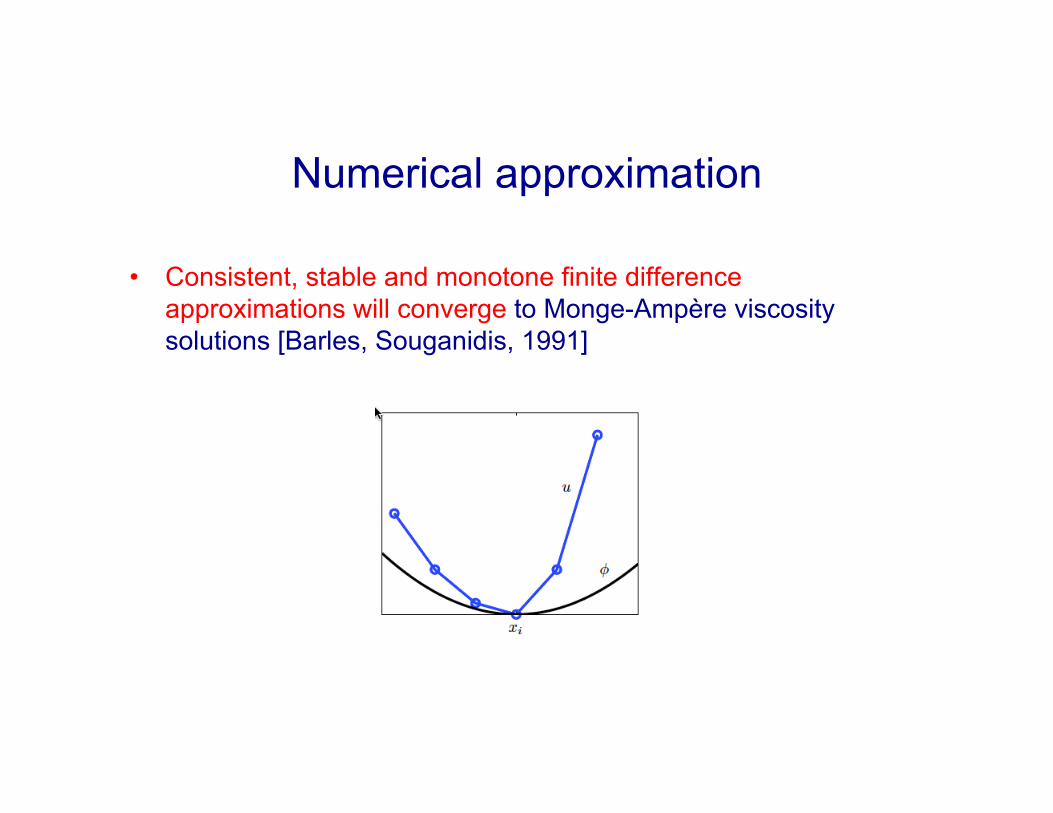
•  Consistent, stable and monotone finite difference approximations will converge to Monge-Ampère viscosity solutions [Barles, Souganidis, 1991]


•  Example, monotone scheme following [Benamou, Froese, Oberman, 2014], discrete maximum principle

uxx ≈ uj+1,k − 2uj,k +uj−1,k( ) /Δx2 monotone

uxv ≈ uj+1,k+1 +uj−1,k−1 −uj+1,k−1 −uj−1,k+1( ) / 4ΔxΔy not monotone

Monotone approximation

det D2u( ) = uvjvj( )j=1

d

∏+

, vj{ } : set of eigenvectors of D2u

Dvv ≈ u(x + vh)− 2u(x)+u(x − vh( ) / vh 2

•  Compare upwind or ENO adaptive stencils and limiters for nonlinear conservation laws •  WENO style smooth

superposition improves Newton convergence

•  MG improves linear solver


•  Final algorithm with filter, almost monotone for higher accuracy (still converging)

•  Newton’s method for discretized nonlinear problem – added regularization in choice of stencil and limiters

4. Applications to waveform inversion and registration

•  Two natural seismic applications for optimal transport and Monge-Ampère –  Measure of mismatch in the inverse problem of finding

velocity: full waveform inversion –  Registration: comparing different datasets

•  Convexity relevant property

Reflections and inversion example

•  Problem with reflection from two layers – dependence on parameters

Offset = R-S

t

R S

Reflections and inversion example

W2

L2

Gradient for optimization

•  For large scale optimization, gradient of J(f) = W22(f,g) with

respect to wave velocity is required in a quasi Newton method in the PDE constrained optimization step

•  Based on linearization of J and Monge-Ampère equation resulting in linear elliptic PDE (adjoint source)

J +δJ = ( f +δ f ) x −∇(uf +δu)∫2dx

f +δ f = g(∇(uf +δu))det(D2 (uf +δu))

L(v) = g(∇uf )tr((D2uf )

•D2 (v))+det(D2uf )g(∇uf )⋅∇v = δ f

Remarks

+ Captures important features of distance in both travel time and L2 + There exists fast algorithms + Robust vs. noise - Constraints that are not natural for seismology

•  Consider positive and negative parts of f and g separately and (regularize) – not appropriate for adjoin field gradient technique

•  Normalize and regularize: add small constant where g = 0 •  Alternative W2: W1 trace by trace W2 (1D)

f (x)dx =X∫ g(y)dy

Y∫ , f , g ≥ 0

g > 0, convex domain

Applications Seismic test cases

•  Marmousi model (velocity field) •  Original model and initial velocity field to start optimization

Marmousi model

•  Original and FWI reconstruction with different initializations: W2-1D, W2-2D, L2

Remark

•  Robustness to noise: good for data but allows for oscillations in “optimal” computed velocity

•  Remedy: trace by trace, TV - regularization

Remark

•  Robustness to noise: good for data but allows for oscillations in “optimal” computed velocity

•  Remedy: trace by trace, TV - regularization

W2

W1

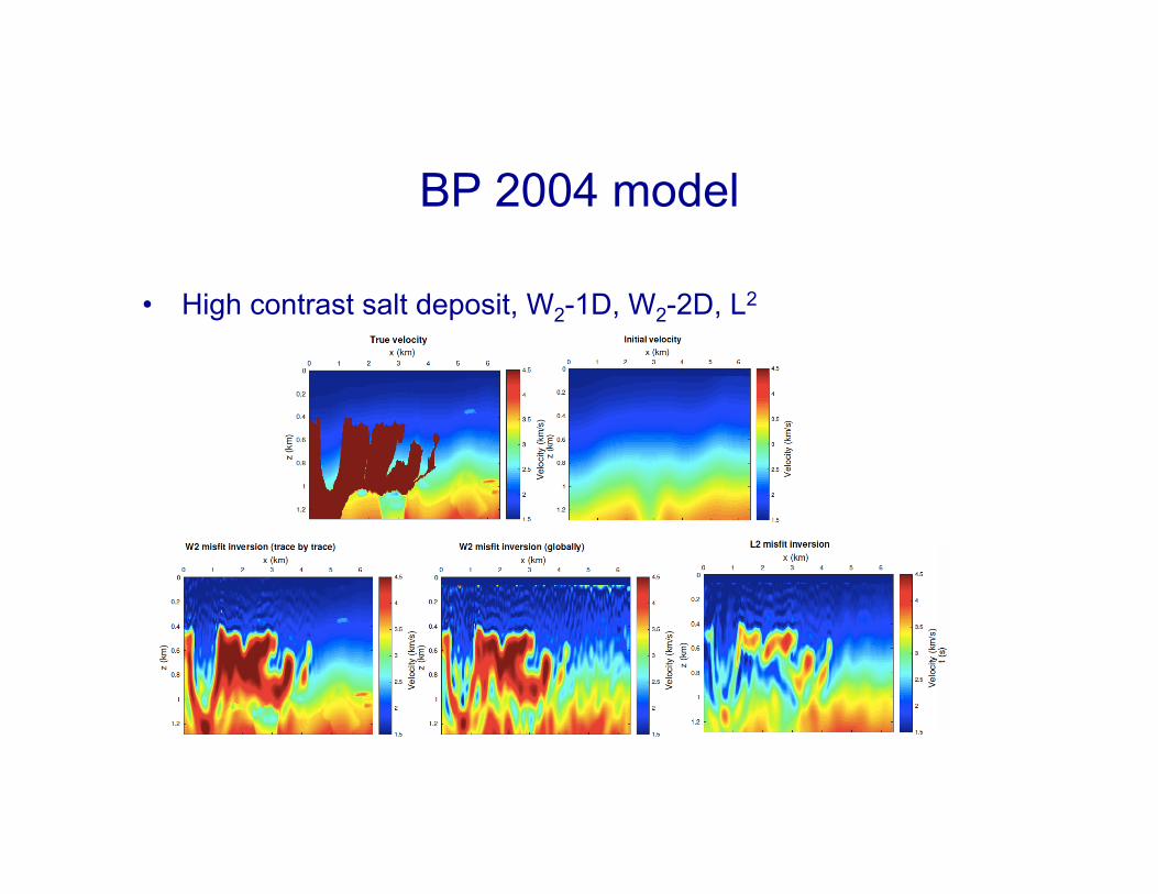
BP 2004 model

•  High contrast salt deposit, W2-1D, W2-2D, L2

Camembert

Additional information from Monge-Ampère solution: T=grad(u) for registration

•  Seismic applications

–  Matching different measurements (well log – seismic) –  Monitor reservoir year by year

•  Common in image processing (often 1D)

Source Target grad(u)-x

Other related work

•  Example below: W1 measure and Marmousi p-velocity model [Metivier etr. Al, 2016]

•  Current optimal transport based development: Schlumberger, Total

Registration

f

g

Registration

f

g

Optimal transport requirements may have unwanted effect on seismic registration

Registration

f

g

Need to modify algorithm

Iteration on truncated signals and maps

Using map based on Monge-Ampère solution for registration

T(x) = grad(u) - x Ta(x) ≈ grad(u) – x smooth, weighted L2

Using map based on Monge-Ampère solution for registration

•  The full algorithms based on cropping data and iterate over updated registered maps •  Applications commonly requires modification to the basic theory

5. Conclusions

•  Improved seismic exploration requires progress in computational mathematics

•  Optimal transport and the Wasserstein metric are promising tools in seismic imaging

•  Theory and basic algorithms need to be substantially modified to handle realistic seismic data:

–  B. Engquist and B. Froese, Application of the Wasserstein metric to seismic signals, Comm. in Math. Sciences, 12. 979-988, 2014

–  B. Engquist, B. Froese and Y. Yang, Optimal transport for Seismic full waveform inversion, to appear

–  Y. Yang, B. Engquist and J. Sun, Convexity of the quadratic Wasserstein metric as a misfit function for full waveform inversion, SEG 2016, subm.

Happy Birthday Yann

bjorn engquist in collaboration with brittany froese ...in collaboration with brittany froese,...

Documents