bis working papers · bis working papers no 487 ... many commentators started to speculate on...

BIS Working PapersNo 487

The biofuel connection: impact of US regulation on oil and food prices by Fernando Avalos and Marco Lombardi

Monetary and Economic Department

February 2015

JEL classification: H23, O13, Q16, Q48.

Keywords: oil price, corn price, food prices, ethanol, biofuel, VAR.

BIS Working Papers are written by members of the Monetary and Economic Department of the Bank for International Settlements, and from time to time by other economists, and are published by the Bank. The papers are on subjects of topical interest and are technical in character. The views expressed in them are those of their authors and not necessarily the views of the BIS.

This publication is available on the BIS website (www.bis.org).

© Bank for International Settlements 2015. All rights reserved. Brief excerpts may be reproduced or translated provided the source is stated.

ISSN 1020-0959 (print) ISSN 1682-7678 (online)

http://www.bis.org/

WP487 The biofuel connection: impact of US regulation on oil and food prices 1

The biofuel connection: impact of US regulation on oil and food prices

Fernando Avalos1 and Marco Lombardi

Abstract

Biofuel policies are frequently mentioned in the policy and academic debates because of their potential impact on food prices. In 2005, the United States authorities passed legislation under which corn-based ethanol became in practice the only available gasoline additive. Some studies have then argued that ethanol and biodiesel subsidies in advanced economies may have strengthened the link between the prices of oil and those of some food commodities. This paper tests whether the response of food commodity prices to global demand shocks and to oil-specific demand shocks has changed following the introduction of this legislation. Our results show that corn prices exhibit a stronger response to global demand shocks after 2006. Some short-lived but statistically significant response to oil-specific demand shocks is also documented. Close substitutes of corn in the feedstock business (eg soybeans and wheat) exhibit comparable but more muted responses, while other food commodities unaffected by biofuel policies do not change their behaviour. We also report some evidence that global liquidity is a factor driving global demand shocks, and through that channel may have affected food commodity prices.

Keywords: oil price, corn price, food prices, ethanol, biofuel, VAR.

JEL classification: H23, O13, Q16, Q48.

1 Corresponding author. Bank for International Settlements, Representative Office for the Americas,

Rubén Darío 281, 11580 Mexico (DF). Tel: +52-55-9138-0292, FAX +52-55-9138-0299. Email: [email protected]. Without implicating, we would like to thank Dubravko Mihaljek, Ramon Moreno and Philip Turner for their helpful comments.

mailto:[email protected]

2 WP487 The biofuel connection: impact of US regulation on oil and food prices

Introduction

The 2000s have seen a broad-based surge of commodities prices, which drove the price of energy, agricultural and metals commodities to record levels; the surge also proved resilient to the Great Recession. However, in the second half of 2014 commodity prices experienced broad-based declines. The forerunner was oil, with prices declining by more than 30% from end-2013 to December 2014. But the prices of other commodities declined too: maize prices, for example, by about 15%. Researchers and market practitioners pointed to several factors explaining these developments: a slowdown in economic growth in commodity-hungry emerging markets, as well as their transition towards less commodity-intensive growth; advances in the exploitation of non-conventional oil sources, which boosted oil production in North America; favourable weather conditions which increased the yield of crops.

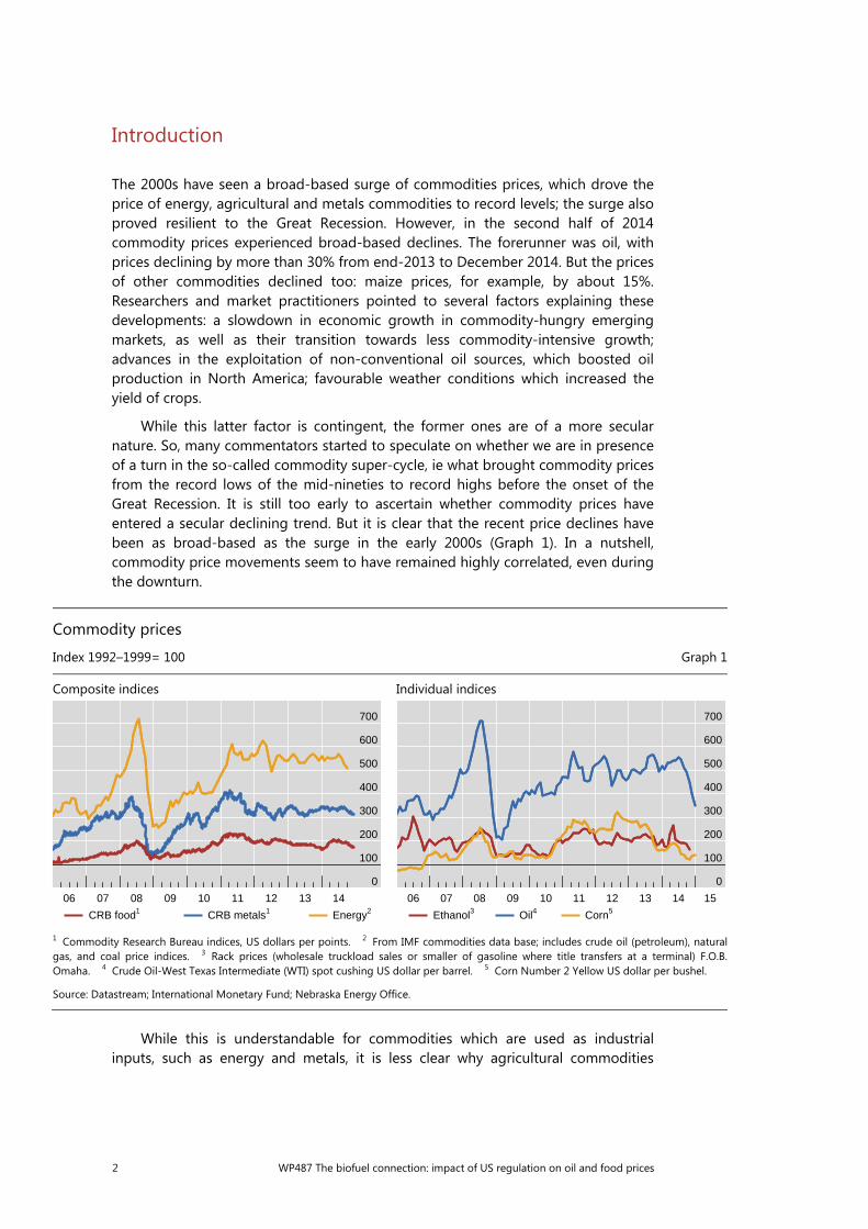
While this latter factor is contingent, the former ones are of a more secular nature. So, many commentators started to speculate on whether we are in presence of a turn in the so-called commodity super-cycle, ie what brought commodity prices from the record lows of the mid-nineties to record highs before the onset of the Great Recession. It is still too early to ascertain whether commodity prices have entered a secular declining trend. But it is clear that the recent price declines have been as broad-based as the surge in the early 2000s (Graph 1). In a nutshell, commodity price movements seem to have remained highly correlated, even during the downturn.

While this is understandable for commodities which are used as industrial inputs, such as energy and metals, it is less clear why agricultural commodities

Commodity prices

Index 1992–1999= 100 Graph 1

Composite indices Individual indices

1 Commodity Research Bureau indices, US dollars per points. 2 From IMF commodities data base; includes crude oil (petroleum), natural gas, and coal price indices. 3 Rack prices (wholesale truckload sales or smaller of gasoline where title transfers at a terminal) F.O.B. Omaha. 4 Crude Oil-West Texas Intermediate (WTI) spot cushing US dollar per barrel. 5 Corn Number 2 Yellow US dollar per bushel.

Source: Datastream; International Monetary Fund; Nebraska Energy Office.

0

100

200

300

400

500

600

700

06 07 08 09 10 11 12 13 14

CRB food1 CRB metals1 Energy2

0

100

200

300

400

500

600

700

06 07 08 09 10 11 12 13 14 15

Ethanol3 Oil4 Corn5


should be correlated with oil prices. Yet the recent literature generally reports significant relationships between oil and some food prices, usually corn, soybeans, and sometimes wheat and rice.2 The direction of causality typically runs from oil to food markets; volatility spillovers from oil to some food markets were also found to be significant in the US after 2006.3

The channels of transmission of oil prices to food commodity prices have also been studied in the literature. The 2011 report of the G20 Study Group on Commodities identified two main channels linking oil and food prices: biofuel production and the growing energy intensity of food production and distribution. In this paper, we are mainly interested in the former channel.

Biofuel promotion policies have been the subject of heated academic and policy debates over the last decade. A key issue has been the perceived risk that such policies may generate additional demand for certain crops and their substitutes, thereby exacerbating upward pressures on food commodity prices. Although biofuel promotion programmes have been in place in some advanced economies since the 1970s, agricultural commodities such as corn, soybeans and sugar did not record sustained price increases until the second half of 2006, when the US Energy Policy Act (EPAct) of 2005 introduced new quantitative standards for the amount of motor fuel coming from renewable sources (see Section 1). As the only cost-effective renewable-source additive to motor fuels is ethanol, which can be produced from a number of food commodities, the observed increase in food commodity prices since 2006 has been sometimes attributed to the introduction of EPAct. This paper tests the hypothesis that this regulation has strengthened the link between oil and food prices in a consistent analytical framework. In addition, the paper studies the channels through which oil prices affect food commodity prices.

Most of the literature on this subject does not relate the analysis to the timing of the 2005 EPAct, so the strength of the results varies depending on the specific sample considered. In addition, discussion of the channels of transmission often abstracts from the identification of the structural shocks driving the observed series: shocks of different nature could transmit through different channels. A notable exception is Baumeister and Kilian (2013), who cast the issue of comovements between oil and food commodity prices into a structural VAR framework.

Our paper contributes to the literature by attempting to assess how oil market structural shocks affect food markets, which food markets are actually impacted, and how that response has changed over time. Moreover, we explore the role of monetary policy in shaping the oil market’s structural shocks, and explore transmission channels different from ethanol. Therefore, our paper is similar in spirit to Baumeister and Kilian (2013), although the framework is somehow different.

More specifically, we build on a structural VAR model of the market for crude oil (Kilian 2009), which disentangles changes in oil prices into shocks to global

2 See for instance Zhang et al (2009), Arshad and Hameed (2009), which identify cointegration

relationships; Nazlioglu (2011), which explores non-linear causality links; Avalos (2014) finds evidence of a 2006 structural break in the covariance matrix of a VAR system including oil, corn and soybean prices.

3 See Trujillo et al (2011), Nazlioglu et al (2012).


demand, oil supply and oil-specific demand factors.4 To examine the response of food prices to such shocks, we add individual food commodity prices to the model. This allows us to control for reverse causality and feedback effects between oil prices and global economic activity, while addressing our main question about the impact of oil-related shocks on food commodity prices. To preserve the identification strategy of Kilian (2009), we abstain from further disentangling demand and supply shocks to individual food commodities.

The paper is organised as follows: Section 1 reviews ethanol-promotion policies in the US and explains why the change introduced in 2006 is particularly relevant. Section 2 presents the data and the model. Section 3 explores the dynamics and linkages of oil and food prices since 2006. Section 4 looks at potential transmission channels of oil price shocks to the prices of food commodities. Section 5 concludes.

1. A regulatory history of ethanol

The use of ethanol as a fuel has a long history in the US. Henry Ford designed the engine of his first automobile to run purely on ethanol. However, the availability of relatively cheap oil resources nudged the car industry towards gasoline. Ethanol production languished in a dormant state for several decades, without completely disappearing. Then the US ethanol industry received a major impulse with the EPAct of 1978, which granted the sector a sizeable tax exemption.5 Ethanol production also benefitted from other state and federal subsidies, as well as heavy tariffs on imported ethanol.

The Clean Air Act of 1990 required gasoline vendors to ensure that their product contained a minimum percentage of oxygen, which improves fuel combustion and reduces emissions. At the time, ethanol was one among several additives that could be mixed with regular gasoline in order to increase its oxygen content. A petroleum or natural gas derivative, methyl tertiary butyl ether or MTBE, was generally much cheaper, more widely available and easier to transport and distribute than ethanol. Consequently, it was preferred in most non-agricultural regions. However, MTBE is highly damaging to the environment and is a known carcinogen for animals. Starting in 2003-04 with the states that were at the time the largest consumers of MTBE (California and New York), several states banned its use within state borders. By 2005, 19 US states had partially or totally banned its use.

The EPAct of 2005 stopped short of a federal ban on the use of MTBE, but introduced a new renewable fuels standard (RFS) to replace the oxygenate standard. RFS required motor fuels to contain a minimum amount of fuel coming from renewable sources, such as biomass (eg ethanol), solar or wind energy. Ethanol offered at the time (and still does) the only practical way to comply with the new

4 For instance, speculative demand triggered by geopolitical uncertainties affecting oil markets, or

substitution effects. 5 The initial exemption was 40 cents per gallon produced. Afterwards, the subsidy ranged between 40

and 60 cents per gallon, irrespective of the price of corn or ethanol. State subsidies frequently doubled the effective subsidy. Federal subsidies were phased out on 31 December 2011. For a more complete description, see Avalos (2014) and references therein.


standard. Therefore, as of mid-2006, ethanol became the only available gasoline additive.

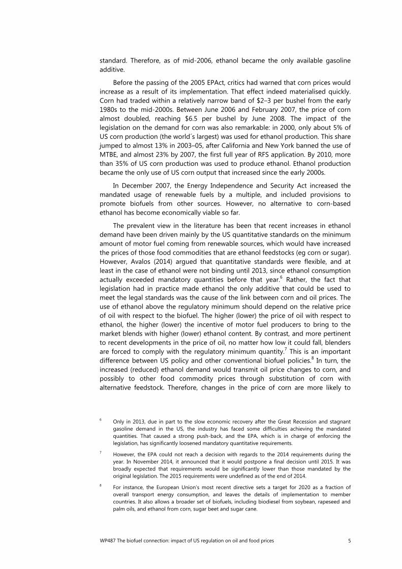
Before the passing of the 2005 EPAct, critics had warned that corn prices would increase as a result of its implementation. That effect indeed materialised quickly. Corn had traded within a relatively narrow band of $2–3 per bushel from the early 1980s to the mid-2000s. Between June 2006 and February 2007, the price of corn almost doubled, reaching $6.5 per bushel by June 2008. The impact of the legislation on the demand for corn was also remarkable: in 2000, only about 5% of US corn production (the world´s largest) was used for ethanol production. This share jumped to almost 13% in 2003–05, after California and New York banned the use of MTBE, and almost 23% by 2007, the first full year of RFS application. By 2010, more than 35% of US corn production was used to produce ethanol. Ethanol production became the only use of US corn output that increased since the early 2000s.

In December 2007, the Energy Independence and Security Act increased the mandated usage of renewable fuels by a multiple, and included provisions to promote biofuels from other sources. However, no alternative to corn-based ethanol has become economically viable so far.

The prevalent view in the literature has been that recent increases in ethanol demand have been driven mainly by the US quantitative standards on the minimum amount of motor fuel coming from renewable sources, which would have increased the prices of those food commodities that are ethanol feedstocks (eg corn or sugar). However, Avalos (2014) argued that quantitative standards were flexible, and at least in the case of ethanol were not binding until 2013, since ethanol consumption actually exceeded mandatory quantities before that year.6 Rather, the fact that legislation had in practice made ethanol the only additive that could be used to meet the legal standards was the cause of the link between corn and oil prices. The use of ethanol above the regulatory minimum should depend on the relative price of oil with respect to the biofuel. The higher (lower) the price of oil with respect to ethanol, the higher (lower) the incentive of motor fuel producers to bring to the market blends with higher (lower) ethanol content. By contrast, and more pertinent to recent developments in the price of oil, no matter how low it could fall, blenders are forced to comply with the regulatory minimum quantity.7 This is an important difference between US policy and other conventional biofuel policies.8 In turn, the increased (reduced) ethanol demand would transmit oil price changes to corn, and possibly to other food commodity prices through substitution of corn with alternative feedstock. Therefore, changes in the price of corn are more likely to

6 Only in 2013, due in part to the slow economic recovery after the Great Recession and stagnant

gasoline demand in the US, the industry has faced some difficulties achieving the mandated quantities. That caused a strong push-back, and the EPA, which is in charge of enforcing the legislation, has significantly loosened mandatory quantitative requirements.

7 However, the EPA could not reach a decision with regards to the 2014 requirements during the year. In November 2014, it announced that it would postpone a final decision until 2015. It was broadly expected that requirements would be significantly lower than those mandated by the original legislation. The 2015 requirements were undefined as of the end of 2014.

8 For instance, the European Union’s most recent directive sets a target for 2020 as a fraction of overall transport energy consumption, and leaves the details of implementation to member countries. It also allows a broader set of biofuels, including biodiesel from soybean, rapeseed and palm oils, and ethanol from corn, sugar beet and sugar cane.


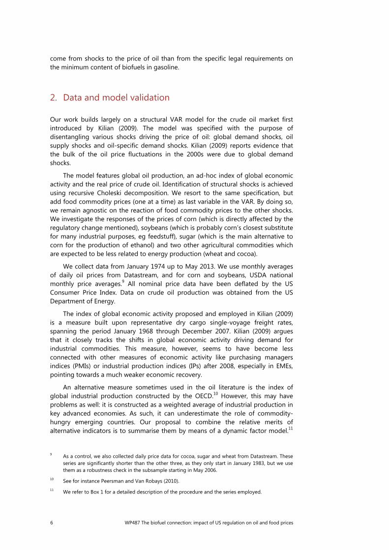
come from shocks to the price of oil than from the specific legal requirements on the minimum content of biofuels in gasoline.

2. Data and model validation

Our work builds largely on a structural VAR model for the crude oil market first introduced by Kilian (2009). The model was specified with the purpose of disentangling various shocks driving the price of oil: global demand shocks, oil supply shocks and oil-specific demand shocks. Kilian (2009) reports evidence that the bulk of the oil price fluctuations in the 2000s were due to global demand shocks.

The model features global oil production, an ad-hoc index of global economic activity and the real price of crude oil. Identification of structural shocks is achieved using recursive Choleski decomposition. We resort to the same specification, but add food commodity prices (one at a time) as last variable in the VAR. By doing so, we remain agnostic on the reaction of food commodity prices to the other shocks. We investigate the responses of the prices of corn (which is directly affected by the regulatory change mentioned), soybeans (which is probably corn’s closest substitute for many industrial purposes, eg feedstuff), sugar (which is the main alternative to corn for the production of ethanol) and two other agricultural commodities which are expected to be less related to energy production (wheat and cocoa).

We collect data from January 1974 up to May 2013. We use monthly averages of daily oil prices from Datastream, and for corn and soybeans, USDA national monthly price averages.9 All nominal price data have been deflated by the US Consumer Price Index. Data on crude oil production was obtained from the US Department of Energy.

The index of global economic activity proposed and employed in Kilian (2009) is a measure built upon representative dry cargo single-voyage freight rates, spanning the period January 1968 through December 2007. Kilian (2009) argues that it closely tracks the shifts in global economic activity driving demand for industrial commodities. This measure, however, seems to have become less connected with other measures of economic activity like purchasing managers indices (PMIs) or industrial production indices (IPs) after 2008, especially in EMEs, pointing towards a much weaker economic recovery.

An alternative measure sometimes used in the oil literature is the index of global industrial production constructed by the OECD.10 However, this may have problems as well: it is constructed as a weighted average of industrial production in key advanced economies. As such, it can underestimate the role of commodity-hungry emerging countries. Our proposal to combine the relative merits of alternative indicators is to summarise them by means of a dynamic factor model.11

9 As a control, we also collected daily price data for cocoa, sugar and wheat from Datastream. These

series are significantly shorter than the other three, as they only start in January 1983, but we use them as a robustness check in the subsample starting in May 2006.

10 See for instance Peersman and Van Robays (2010). 11 We refer to Box 1 for a detailed description of the procedure and the series employed.


In Graph 2 we plot our measure against Kilian´s index, as well as against the OECD’s global industrial production index.12 Being a form of weighted average, it is not surprising that our factor-based measure has similar dynamics to the others while being less volatile. Compared to both the Kilian index and the global industrial production index, our measure indicates a relatively higher level of activity after 2008, and a steeper contraction before.

This being said, to validate our identification strategy, as well as the newly-built index of economic activity, we estimated a VAR model following the specification of Kilian (2009), adding real corn prices, our main variable of interest among agricultural commodities, as last variable in the system. This is intended to verify that the results reported by Kilian (2009) are robust to the inclusion of an additional variable and the use of an alternative measure of economic activity.

More formally, we estimated a VAR on monthly data from January 1974 up to May 2013 featuring, in order: the monthly percentage change in oil production (∆ ), the dynamic factor described above as proxy of global activity ( ), the logarithm of the real price of oil ( _ ), and the logarithm of the real price of corn ( _ ). The structural VAR representation of = ∆ , , _ , _ ′ is then the following:

= + + , where is the vector of serially and mutually uncorrelated structural shocks. We assume that the matrix has a recursive structure. This allows us to factorize the errors of the estimated reduced-form model as follows: =

12 To facilitate the comparison, all series were standardised.

Comparison between Kilian (2009) real economic activity index, the dynamic factor index and OECD industrial production index

Standardized variables Graph 2

Source: BIS calculations.

–6

–4

–2

0

2

01 03 05 07 09 11 13

Real economic activity index Dynamic factor index Industrial production for OECD members


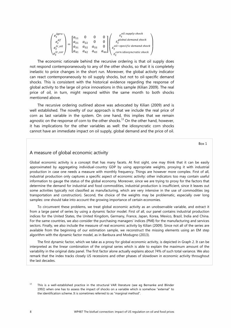
∆__ = 0 0 00 00

The economic rationale behind the recursive ordering is that oil supply does not respond contemporaneously to any of the other shocks, so that it is completely inelastic to price changes in the short run. Moreover, the global activity indicator can react contemporaneously to oil supply shocks, but not to oil-specific demand shocks. This is consistent with the historical evidence regarding the response of global activity to the large oil price innovations in this sample (Kilian 2009). The real price of oil, in turn, might respond within the same month to both shocks mentioned above.

The recursive ordering outlined above was advocated by Kilian (2009) and is well established. The novelty of our approach is that we include the real price of corn as last variable in the system. On one hand, this implies that we remain agnostic on the response of corn to the other shocks.13 On the other hand, however, it has implications for the other variables as well: the idiosyncratic corn shocks cannot have an immediate impact on oil supply, global demand and the price of oil.

Box 1

A measure of global economic activity

Global economic activity is a concept that has many facets. At first sight, one may think that it can be easily approximated by aggregating individual-country GDP by using appropriate weights, proxying it with industrial production in case one needs a measure with monthly frequency. Things are however more complex. First of all, industrial production only captures a specific aspect of economic activity: other indicators too may contain useful information to gauge the status of the global economy. Moreover, since we are trying to proxy for the factors that determine the demand for industrial and food commodities, industrial production is insufficient, since it leaves out some activities typically not classified as manufacturing, which are very intensive in the use of commodities (eg transportation and construction). Second, the choice of the weights may be problematic, especially over long samples: one should take into account the growing importance of certain economies.

To circumvent these problems, we treat global economic activity as an unobservable variable, and extract it from a large panel of series by using a dynamic factor model. First of all, our panel contains industrial production indices for the United States, the United Kingdom, Germany, France, Japan, Korea, Mexico, Brazil, India and China. For the same countries, we also consider the purchasing managers’ indices (PMI) for the manufacturing and services sectors. Finally, we also include the measure of real economic activity by Kilian (2009). Since not all of the series are available from the beginning of our estimation sample, we reconstruct the missing elements using an EM step algorithm with the dynamic factor model, as in Banbura and Modugno (2013).

The first dynamic factor, which we take as a proxy for global economic activity, is depicted in Graph 2. It can be interpreted as the linear combination of the original series which is able to explain the maximum amount of the variability in the original data panel. The first factor alone actually explains about 74% of such total variance. We also remark that the index tracks closely US recessions and other phases of slowdown in economic activity throughout the last decades.

13 This is a well-established practice in the structural VAR literature (see eg Bernanke and Blinder

1992) when one has to assess the impact of shocks on a variable which is somehow “external” to the identification scheme. It is sometimes referred to as “marginal method”.


Whereas for the former two variables the assumption sounds reasonable, it may be restrictive in what concerns the response of the oil price. After all, both prices are set in continuously active financial markets, and they are likely to influence each other. To check for the robustness of our results to this assumption, we tried switching the ordering of oil and corn prices in the system, and the results were substantially unchanged.

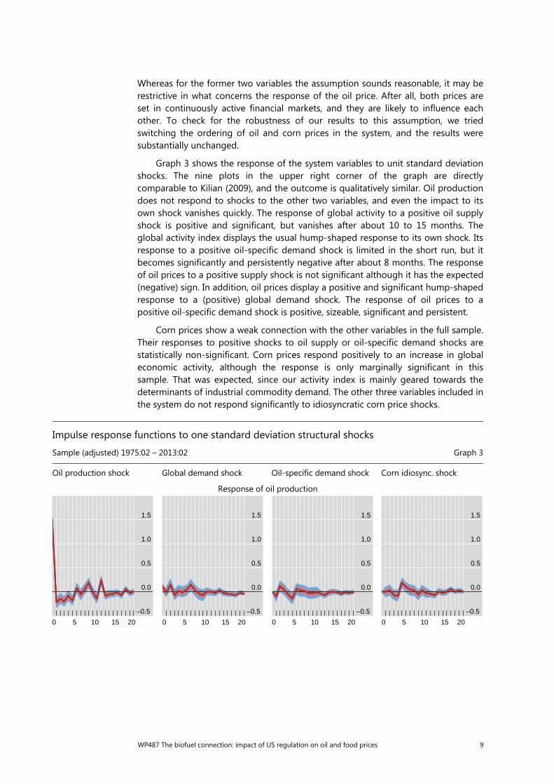
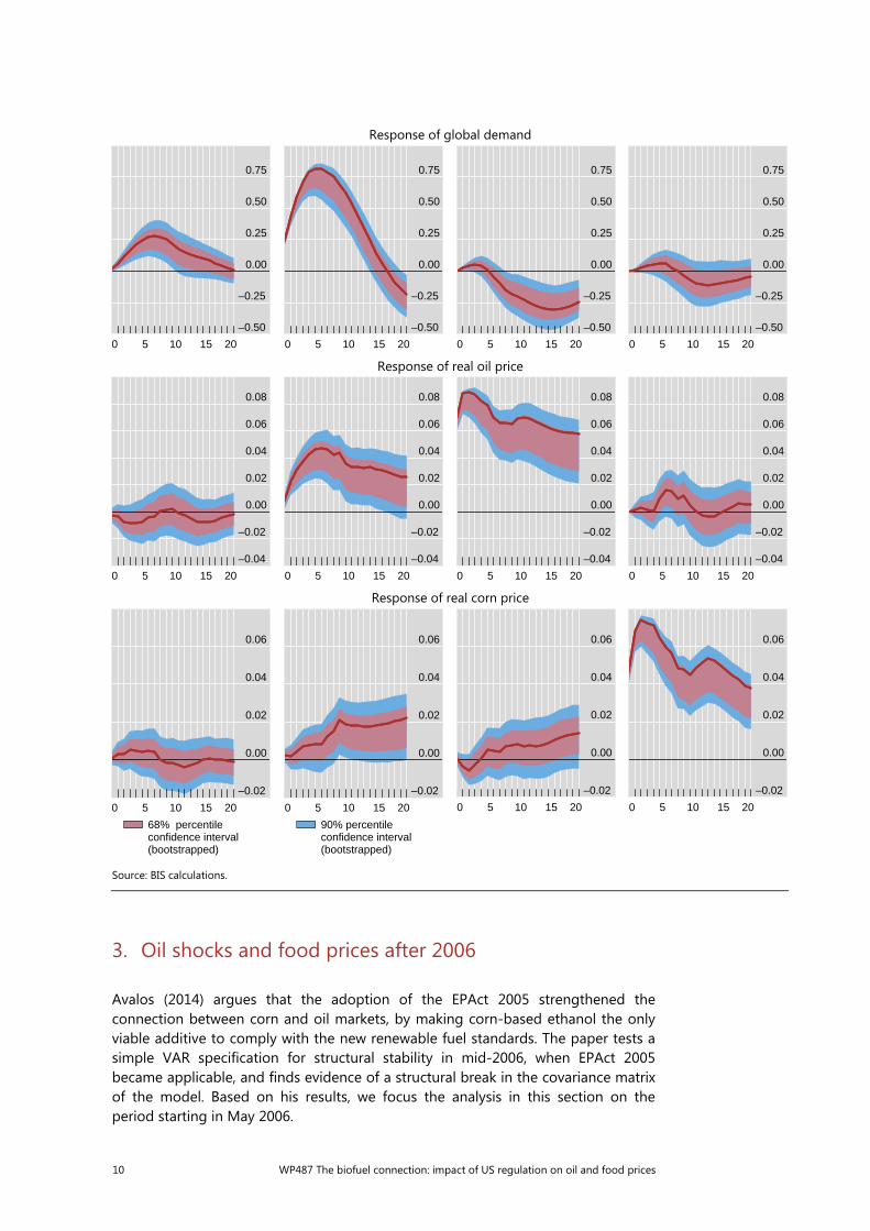
Graph 3 shows the response of the system variables to unit standard deviation shocks. The nine plots in the upper right corner of the graph are directly comparable to Kilian (2009), and the outcome is qualitatively similar. Oil production does not respond to shocks to the other two variables, and even the impact to its own shock vanishes quickly. The response of global activity to a positive oil supply shock is positive and significant, but vanishes after about 10 to 15 months. The global activity index displays the usual hump-shaped response to its own shock. Its response to a positive oil-specific demand shock is limited in the short run, but it becomes significantly and persistently negative after about 8 months. The response of oil prices to a positive supply shock is not significant although it has the expected (negative) sign. In addition, oil prices display a positive and significant hump-shaped response to a (positive) global demand shock. The response of oil prices to a positive oil-specific demand shock is positive, sizeable, significant and persistent.

Corn prices show a weak connection with the other variables in the full sample. Their responses to positive shocks to oil supply or oil-specific demand shocks are statistically non-significant. Corn prices respond positively to an increase in global economic activity, although the response is only marginally significant in this sample. That was expected, since our activity index is mainly geared towards the determinants of industrial commodity demand. The other three variables included in the system do not respond significantly to idiosyncratic corn price shocks.

Impulse response functions to one standard deviation structural shocks

Sample (adjusted) 1975:02 – 2013:02 Graph 3

Oil production shock Global demand shock Oil-specific demand shock Corn idiosync. shock

Response of oil production

–0.5

0.0

0.5

1.0

1.5

0 5 10 15 20

–0.5

0.0

0.5

1.0

1.5

0 5 10 15 20

–0.5

0.0

0.5

1.0

1.5

0 5 10 15 20

–0.5

0.0

0.5

1.0

1.5

0 5 10 15 20


Response of global demand

Response of real oil price

Response of real corn price


3. Oil shocks and food prices after 2006

Avalos (2014) argues that the adoption of the EPAct 2005 strengthened the connection between corn and oil markets, by making corn-based ethanol the only viable additive to comply with the new renewable fuel standards. The paper tests a simple VAR specification for structural stability in mid-2006, when EPAct 2005 became applicable, and finds evidence of a structural break in the covariance matrix of the model. Based on his results, we focus the analysis in this section on the period starting in May 2006.

–0.50

–0.25

0.00

0.25

0.50

0.75

0 5 10 15 20

–0.50

–0.25

0.00

0.25

0.50

0.75

0 5 10 15 20

–0.50

–0.25

0.00

0.25

0.50

0.75

0 5 10 15 20

–0.50

–0.25

0.00

0.25

0.50

0.75

0 5 10 15 20

–0.04

–0.02

0.00

0.02

0.04

0.06

0.08

0 5 10 15 20

–0.04

–0.02

0.00

0.02

0.04

0.06

0.08

0 5 10 15 20

–0.04

–0.02

0.00

0.02

0.04

0.06

0.08

0 5 10 15 20

–0.04

–0.02

0.00

0.02

0.04

0.06

0.08

0 5 10 15 20

–0.02

0.00

0.02

0.04

0.06

0 5 10 15 20

68% percentile confidence interval (bootstrapped)

–0.02

0.00

0.02

0.04

0.06

0 5 10 15 20


–0.02

0.00

0.02

0.04

0.06

0 5 10 15 20

–0.02

0.00

0.02

0.04

0.06

0 5 10 15 20


The first step of our analysis is to estimate a structural VAR akin to the one presented in the previous section. More specifically, we augment the system proposed by Kilian (2009) by adding real corn prices as last variable. In this case, since we have a much smaller sample size, we choose the lag order by resorting to information criteria, rather than using 12 or 24 lags as is commonplace in the literature. All criteria (Akaike, Schwarz and Hannan-Quinn) suggest the use of a 2-lag structure for this sample. We therefore maintain this lag structure for all the models in the following sections.

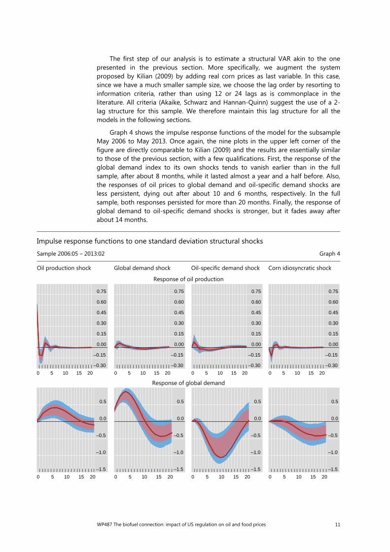
Graph 4 shows the impulse response functions of the model for the subsample May 2006 to May 2013. Once again, the nine plots in the upper left corner of the figure are directly comparable to Kilian (2009) and the results are essentially similar to those of the previous section, with a few qualifications. First, the response of the global demand index to its own shocks tends to vanish earlier than in the full sample, after about 8 months, while it lasted almost a year and a half before. Also, the responses of oil prices to global demand and oil-specific demand shocks are less persistent, dying out after about 10 and 6 months, respectively. In the full sample, both responses persisted for more than 20 months. Finally, the response of global demand to oil-specific demand shocks is stronger, but it fades away after about 14 months.

Impulse response functions to one standard deviation structural shocks

Sample 2006:05 – 2013:02 Graph 4

Oil production shock Global demand shock Oil-specific demand shock Corn idiosyncratic shock



–0.30

–0.15

0.00

0.15

0.30

0.45

0.60

0.75

0 5 10 15 20

–0.30

–0.15

0.00

0.15

0.30

0.45

0.60

0.75

0 5 10 15 20

–0.30

–0.15

0.00

0.15

0.30

0.45

0.60

0.75

0 5 10 15 20

–0.30

–0.15

0.00

0.15

0.30

0.45

0.60

0.75

0 5 10 15 20

–1.5

–1.0

–0.5

0.0

0.5

0 5 10 15 20

–1.5

–1.0

–0.5

0.0

0.5

0 5 10 15 20

–1.5

–1.0

–0.5

0.0

0.5

0 5 10 15 20

–1.5

–1.0

–0.5

0.0

0.5

0 5 10 15 20


Looking more closely at corn prices, the responses of oil production, global demand, and real oil prices to a positive (unit standard deviation) idiosyncratic corn price shock are comparable to those in the full sample (essentially non-significant). There are some relevant changes in the response of corn prices to the other structural shocks. There is now a stronger positive response to a positive shock to the global demand factors that drive the demand for industrial commodities, which is significant from the beginning and vanishes after about 20 months. Also, there is a significant initial positive response to a positive oil-specific demand shock, but it disappears almost immediately. The response of corn prices to their own idiosyncratic shocks is initially stronger, but it starts to decline after one period (it was more hump-shaped in the full sample) and peters out after about 20 months, whereas in the full sample the response lasted well beyond 20 months.

In Graph 5 we report the variance decomposition of corn prices over 12 and 18 month horizons for both the full sample and the post-May 2006 subsample. The contribution of structural shocks to global demand and oil-specific demand to the forecast errors of corn prices are much higher than in the full sample. Moreover, the contribution of corn idiosyncratic shocks to the forecast errors dropped from around 95% in the full sample, to slightly more than 70% in the post-May 2006 subsample, with the difference going to oil market shocks.




–0.075

–0.050

–0.025

0.000

0.025

0.050

0.075

0 5 10 15 20

–0.075

–0.050

–0.025

0.000

0.025

0.050

0.075

0 5 10 15 20

–0.075

–0.050

–0.025

0.000

0.025

0.050

0.075

0 5 10 15 20

–0.075

–0.050

–0.025

0.000

0.025

0.050

0.075

0 5 10 15 20

–0.06

–0.04

–0.02

0.00

0.02

0.04

0.06

0 5 10 15 20


–0.06

–0.04

–0.02

0.00

0.02

0.04

0.06

0 5 10 15 20

90% percentile confidence interval(bootstrapped)

–0.06

–0.04

–0.02

0.00

0.02

0.04

0.06

0 5 10 15 20

–0.06

–0.04

–0.02

0.00

0.02

0.04

0.06

0 5 10 15 20


This being established, we append real soybean prices at the end of the augmented system, to start the analysis of the effect of oil price changes on other food commodities. Soybeans are sometimes used as feedstock for biodiesel production, but they cannot be used to produce ethanol, so the impact of EPAct 2005 on their prices can only be indirect, most likely through the impact on corn prices. In other words, higher corn prices will increase soybean demand in the short run (by substituting pricier corn for soybean in industrial uses) and/or reduce its supply in the long run (by encouraging the expansion of acreage planted with corn instead of soybeans).14 It is important to distinguish between the response to oil-related shocks and corn idiosyncratic shocks, which is the reason why we append soybean prices at the end of the augmented model, rather than simply substituting corn with soybeans. Taking this latter road will confound the response to different types of structural shocks.15

The impulse response functions for such an extended system reveal that the results for oil production, global demand, oil and corn real prices are qualitatively and quantitatively unchanged from those presented in Graph 4. Moreover, the responses of those four variables to soybean idiosyncratic shocks are statistically (and economically) non-significant.16 Therefore, the only interesting dynamics are on the responses of soybean prices to the structural shocks, summarised in the impulse response functions reported in Graph 6. The real price of soybeans displays a non-significant response to a positive unit standard deviation shock to oil production. The response to a similar shock in global demand is marginally statistically significant but lasts over 20 months, whereas the response to an oil-specific demand shock is quantitatively comparable initially, but disappears after about 3 months. So the bulk of the dynamics for soybean prices is concentrated in

14 See Hausman et al (2012) for estimations of the price impact of changes in acreage for different

crops. 15 In the next section, we also conduct some robustness checks by replacing the price of soybean for

other food commodities. 16 In the interest of saving space, we only report a subset of those results in the next section. The

complete set of results is available from the authors upon request.

Forecast error variance decomposition of corn prices Graph 5

In per cent


0

20

40

60

80

100

Up to 12 months Up to 18 months Up to 12 months Up to 18 months

Full sample Short sample

Oil production change Log of real price of oil Log of real price of corn Global demand


the response to corn and their own idiosyncratic shocks. In fact, the response to corn idiosyncratic shocks seem quantitatively larger and more persistent, levelling out after about 20 months, whilst the response to soybean prices’ own idiosyncratic shocks decreases more quickly, becoming statistically insignificant after about 10 months. Corn and soybean idiosyncratic shocks account for more than 80% of soybean prices’ forecast errors within an 18-month horizon.

3.1 Robustness checks

In this section, we present some evidence on the robustness of our findings. Rather than changing the identification strategy, we replace soybeans for other crops in the extended model. This serves a twofold purpose: verify the resilience of the dynamic interactions presented so far, and investigate how (if at all) other food commodity markets were affected by oil market gyrations in the post-May 2006 period.

We introduce three new crops: wheat, sugar and cocoa. Wheat is also a substitute for corn and soybeans in some industrial applications. However, wheat cannot be used in the production of any sort of biofuel, so the impact of oil price changes on its prices must be only indirect, through substitution for corn in industrial use or planted acreage. In addition, climate requirements for wheat and corn are not identical, and the acreage substitution from wheat to corn is more limited than in the case of soybeans. All this suggests that the response of wheat prices to the structural shocks discussed so far is likely to be more restrained. Sugar is the main feedstock for the production of ethanol in Brazil, which potentially could have competed with domestic US corn-based ethanol, thereby creating a transmission channel between those markets. Nevertheless, high import tariffs during most of our sample period reduced sugarcane-based ethanol to a marginal player in the US domestic ethanol market. Finally, cocoa has no direct or indirect connection with the biofuel industry.

Impulse response functions of soybean prices to one standard deviation structural shocks

Sample 2006:05 – 2013:02 Graph 6



–0.04

–0.03

–0.02

–0.01

0.00

0.01

0.02

0.03

0.04

0 5 10 15 20


–0.04

–0.03

–0.02

–0.01

0.00

0.01

0.02

0.03

0.04

0 5 10 15 20


–0.04

–0.03

–0.02

–0.01

0.00

0.01

0.02

0.03

0.04

0 5 10 15 20

–0.04

–0.03

–0.02

–0.01

0.00

0.01

0.02

0.03

0.04

0 5 10 15 20


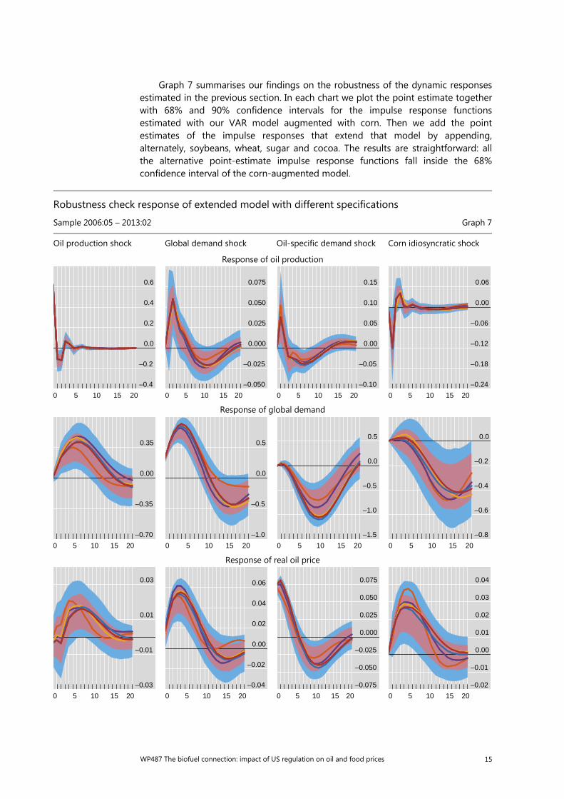
Graph 7 summarises our findings on the robustness of the dynamic responses estimated in the previous section. In each chart we plot the point estimate together with 68% and 90% confidence intervals for the impulse response functions estimated with our VAR model augmented with corn. Then we add the point estimates of the impulse responses that extend that model by appending, alternately, soybeans, wheat, sugar and cocoa. The results are straightforward: all the alternative point-estimate impulse response functions fall inside the 68% confidence interval of the corn-augmented model.

Robustness check response of extended model with different specifications

Sample 2006:05 – 2013:02 Graph 7





–0.4

–0.2

0.0

0.2

0.4

0.6

0 5 10 15 20

–0.050

–0.025

0.000

0.025

0.050

0.075

0 5 10 15 20

–0.10

–0.05

0.00

0.05

0.10

0.15

0 5 10 15 20

–0.24

–0.18

–0.12

–0.06

0.00

0.06

0 5 10 15 20

–0.70

–0.35

0.00

0.35

0 5 10 15 20

–1.0

–0.5

0.0

0.5

0 5 10 15 20

–1.5

–1.0

–0.5

0.0

0.5

0 5 10 15 20

–0.8

–0.6

–0.4

–0.2

0.0

0 5 10 15 20

–0.03

–0.01

0.01

0.03

0 5 10 15 20

–0.04

–0.02

0.00

0.02

0.04

0.06

0 5 10 15 20

–0.075

–0.050

–0.025

0.000

0.025

0.050

0.075

0 5 10 15 20

–0.02

–0.01

0.00

0.01

0.02

0.03

0.04

0 5 10 15 20


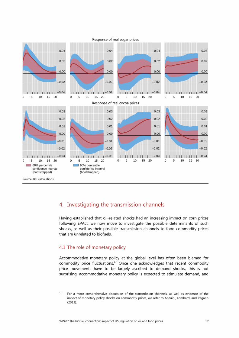
Next, we focus on the specific responses of each crop to unit standard deviation shocks in each of the structural innovations. Graph 8 presents those results. The upper row corresponds to the responses of real wheat prices, which show no statistically significant reaction to oil production or global demand shocks. There is a stronger but fleeting response to oil-specific demand shocks that vanishes after two months, and a stronger reaction to corn price shocks, that also disappears after about 6 months. The responses of sugar prices are presented in the middle row of Graph 8. There is an initially positive but marginally significant response to global demand shocks, which lasts about three months before vanishing. The response of sugar prices to oil supply shocks is quantitatively and statistically stronger, fading away after about 7 months. Moreover, the response of real sugar prices to oil-specific demand shocks or corn idiosyncratic shocks is nil. Finally, the bottom row of Graph 8 shows that cocoa prices display a brief but relatively strong positive response to a positive idiosyncratic shock to corn prices, and weaker and mostly non-statistically significant responses to oil production, global demand and oil specific demand shocks.

Impulse response of other food commodities to one standard deviation structural shocks

Sample 2006:05 – 2013:02 Graph 8


Response of real wheat prices

–0.04

–0.02

0.00

0.02

0.04

0.06

0 5 10 15 20

–0.04

–0.02

0.00

0.02

0.04

0.06

0 5 10 15 20

–0.04

–0.02

0.00

0.02

0.04

0.06

0 5 10 15 20

–0.04

–0.02

0.00

0.02

0.04

0.06

0 5 10 15 20



–0.030

–0.015

0.000

0.015

0 5 10 15 20

68% percentile condifence interval(bootstrapped)

–0.02

0.00

0.02

0.04

0 5 10 15 20

90% percentile condifence interval(bootstrapped)

–0.06

–0.03

0.00

0.03

0 5 10 15 20

Base modelModel with soybeanModel with cocoa

–0.025

0.000

0.025

0.050

0 5 10 15 20

Model with sugarModel with wheat


4. Investigating the transmission channels

Having established that oil-related shocks had an increasing impact on corn prices following EPAct, we now move to investigate the possible determinants of such shocks, as well as their possible transmission channels to food commodity prices that are unrelated to biofuels.

4.1 The role of monetary policy

Accommodative monetary policy at the global level has often been blamed for commodity price fluctuations.17 Once one acknowledges that recent commodity price movements have to be largely ascribed to demand shocks, this is not surprising: accommodative monetary policy is expected to stimulate demand, and

17 For a more comprehensive discussion of the transmission channels, as well as evidence of the

impact of monetary policy shocks on commodity prices, we refer to Anzuini, Lombardi and Pagano (2013).

Response of real sugar prices

Response of real cocoa prices


–0.04

–0.02

0.00

0.02

0.04

0 5 10 15 20

–0.04

–0.02

0.00

0.02

0.04

0 5 10 15 20

–0.04

–0.02

0.00

0.02

0.04

0 5 10 15 20

–0.04

–0.02

0.00

0.02

0.04

0 5 10 15 20

–0.03

–0.02

–0.01

0.00

0.01

0.02

0.03

0 5 10 15 20


–0.03

–0.02

–0.01

0.00

0.01

0.02

0.03

0 5 10 15 20


–0.03

–0.02

–0.01

0.00

0.01

0.02

0.03

0 5 10 15 20

–0.03

–0.02

–0.01

0.00

0.01

0.02

0.03

0 5 10 15 20


hence push commodity prices upwards. However, there are other possible channels of transmission of monetary policy to commodity prices. Low interest rates create incentives for the accumulation of inventories by reducing the opportunity cost of holding them (the cost of carry). Moreover, for extractive minerals, low interest rates also generate incentives to postpone extraction, thereby restricting the supply to physical markets. The implication, in both cases, is that low interest rates would tend to increase oil prices. Finally, the increasing appetite for commodity-related investment products may well be related to low interest rates at the global level, which encourage investors to seek alternative sources of yield.18 Large inflows of funds into commodity futures, in turn, may also push commodity prices upwards (financial channel).19

Our VAR does not explicitly model monetary policy, therefore its impact could materialise in the various structural shocks: if global demand is stimulated by a monetary policy loosening, a measure of monetary policy should partially explain global demand shocks. If, on the other hand, monetary policy affects commodity prices through the inventory channel or the financial channel, we expect it to explain oil-specific demand shocks. Finally, if extraction postponement is a relevant transmission channel, looser monetary policy could also result in oil production drops.

To test for this, we extracted the structural shocks from the VAR model of the previous section and regressed them on the measure of global liquidity proposed by Eickmeier, Gambacorta and Hofmann (2013). We acknowledge that using such an estimate of global liquidity has caveats. However, we think that given the global nature of shocks in the model, a country-specific measure is not sufficient to account for the global monetary policy stance. The use of single-country measures would fail to account for liquidity spillovers to other markets, in particular to the large emerging market economies that have been driving the demand for commodities in recent years.20 Moreover, the unconventional nature of many of the monetary policy measures that dominate our sample period makes more traditional measures of policy stance (eg deviations of the Fed Funds rates from a Taylor rule) less informative and reliable.21

The global liquidity measure is quarterly, ranging from 1Q 1996 through 2Q 2011. Higher levels of this measure are associated with tighter liquidity conditions. Our estimated structural shocks are monthly, and we sum them over the quarter to meet the periodicity of the global liquidity indicator (GLI). We then regress each structural shock on a constant and the GLI. Results are reported in Table 1 and suggest, consistent with Anzuini et al (2013), that the only significant channel seems to be that of global demand: its GLI coefficient is statistically significant even at the 1% level, while the other coefficients’ significance cannot be accepted at any reasonable level. The failure of GLI to explain any of the other structural shocks

18 See Frankel and Rose (2010) for a more detailed discussion. 19 However, empirical evidence of this is, at best, scant. We refer to Lombardi and Van Robays (2011)

and Fattouh, Kilian and Mahadeva (2012) for an overview. 20 See, for instance, Aastveit et al (2012) for evidence on this matter. 21 We indeed cross-checked our results using the US Federal Funds Rate in place of the global

liquidity measure, and found that results are no longer significant.


suggests that the role of the financial channel, the extraction postponement channel or the inventory channel may be limited.

4.2 Fertilizers, transportation and other transmission channels

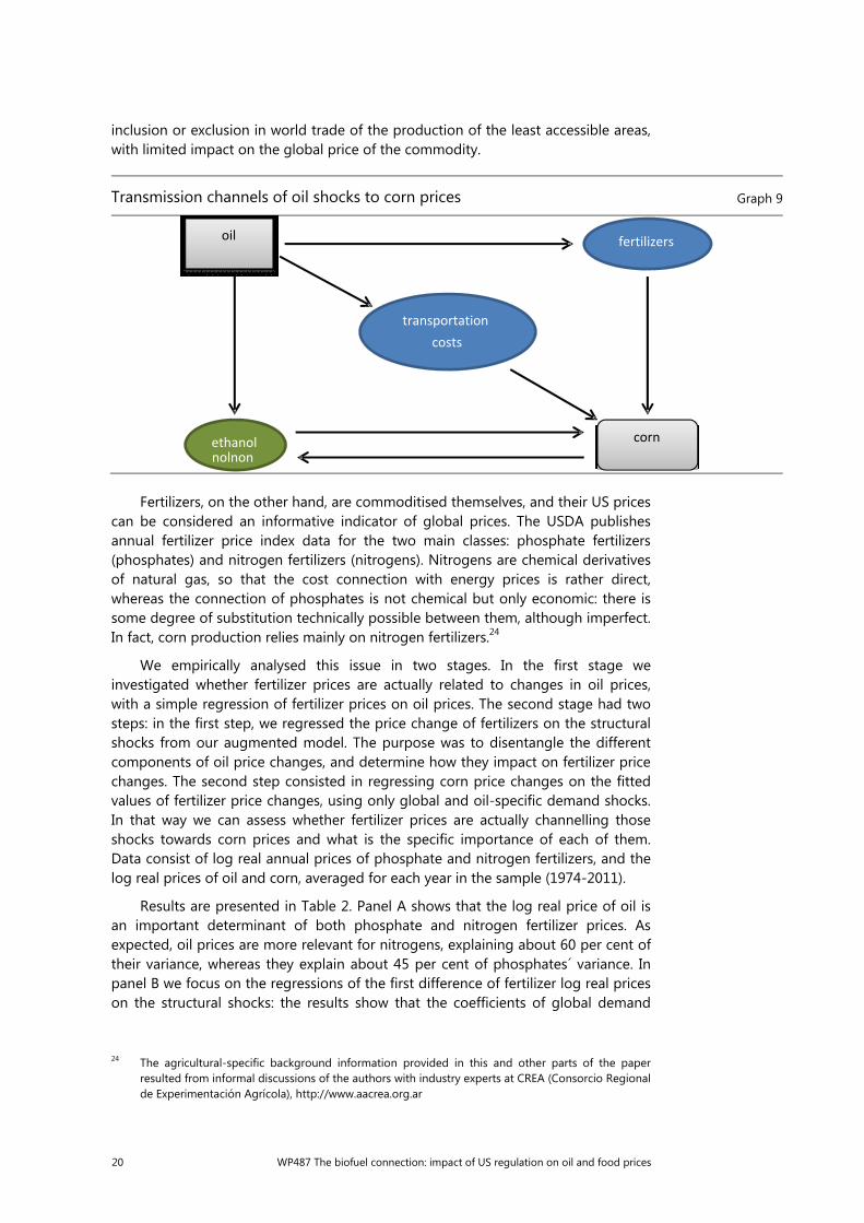
It is often argued that oil prices can affect food commodity prices through channels unrelated to biofuels, but rather to the costs of producing and distributing them: for instance, the growing reliance of modern agriculture on seed fertilizers that are highly dependent on chemical inputs derived from oil. Moreover, the progressive extension of the agricultural frontier to lands far away from port and storage facilities would increase the cost component of transportation, adding substantial cost pressures to market prices.22 The relevance of such cost factors will depend crucially on the specific details of each crop production characteristics. As an example, Graph 9 summarises the ethanol and cost transmission channels between oil and corn prices usually assumed. Notice that there would be a feedback link between ethanol and corn prices: changes in the price of oil can affect ethanol demand (and potentially its price) and that can eventually impact on corn prices, as already discussed. But shocks to corn prices can also affect the ethanol market, because of obvious cost considerations.23 However, there is no empirical evidence supporting a feedback from ethanol to oil prices. In studying the direct connection between oil and corn prices, we exploit this empirical feature to by-pass the additional econometric complication of having to deal with the feedback between corn and ethanol prices.

We were not able to find fare data for bulk land transportation of food commodities. However, since transportation costs are a very idiosyncratic factor, it is not clear that a measure for the United States, if it existed, would help in explaining the price dynamics of a globally traded commodity like corn. Moreover, for a given price of corn, fluctuations in transportation costs are more likely to cause the

22 See, for instance, Arshad and Hameed (2009). 23 See Zhang et al (2009), Trujillo-Barrera et al (2011).

Regression results of structural shocks on global liquidity1,2

Sample 1996:01 - 2011:02 Table 1

Independent variables

Dependent variables

Oil production Global demand Oil-specific demand Corn

Constant 0.016 [0.331]

0.009 [0.110]

0.055 [0.716]

-0.063 [-1.012]

Global liquidity

0.007 [0.320]

-0.104***

[-2.693]

-0.013 [-0.367]

-0.001 [-0.052]

R2 0.002 0.108 0.002 0.000 Adjusted R2 -0.015 0.093 -0.014 -0.017 1 *, **, *** Significance at 10%, 5% and 1%, respectively. 2 t-Statistic between [ ].


inclusion or exclusion in world trade of the production of the least accessible areas, with limited impact on the global price of the commodity.

Fertilizers, on the other hand, are commoditised themselves, and their US prices can be considered an informative indicator of global prices. The USDA publishes annual fertilizer price index data for the two main classes: phosphate fertilizers (phosphates) and nitrogen fertilizers (nitrogens). Nitrogens are chemical derivatives of natural gas, so that the cost connection with energy prices is rather direct, whereas the connection of phosphates is not chemical but only economic: there is some degree of substitution technically possible between them, although imperfect. In fact, corn production relies mainly on nitrogen fertilizers.24

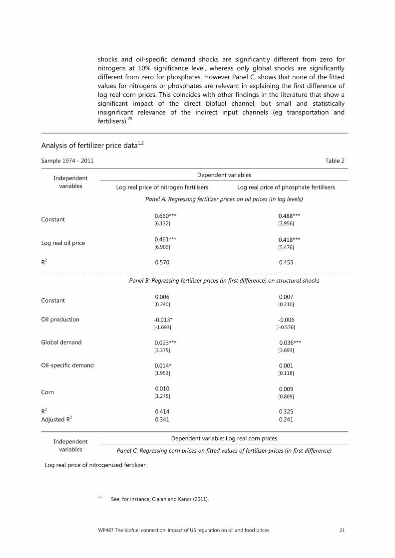
We empirically analysed this issue in two stages. In the first stage we investigated whether fertilizer prices are actually related to changes in oil prices, with a simple regression of fertilizer prices on oil prices. The second stage had two steps: in the first step, we regressed the price change of fertilizers on the structural shocks from our augmented model. The purpose was to disentangle the different components of oil price changes, and determine how they impact on fertilizer price changes. The second step consisted in regressing corn price changes on the fitted values of fertilizer price changes, using only global and oil-specific demand shocks. In that way we can assess whether fertilizer prices are actually channelling those shocks towards corn prices and what is the specific importance of each of them. Data consist of log real annual prices of phosphate and nitrogen fertilizers, and the log real prices of oil and corn, averaged for each year in the sample (1974-2011).

Results are presented in Table 2. Panel A shows that the log real price of oil is an important determinant of both phosphate and nitrogen fertilizer prices. As expected, oil prices are more relevant for nitrogens, explaining about 60 per cent of their variance, whereas they explain about 45 per cent of phosphates´ variance. In panel B we focus on the regressions of the first difference of fertilizer log real prices on the structural shocks: the results show that the coefficients of global demand

24 The agricultural-specific background information provided in this and other parts of the paper

resulted from informal discussions of the authors with industry experts at CREA (Consorcio Regional de Experimentación Agrícola), http://www.aacrea.org.ar

Transmission channels of oil shocks to corn prices Graph 9

oil

corn ethanolnolnon

transportationcosts

fertilizers


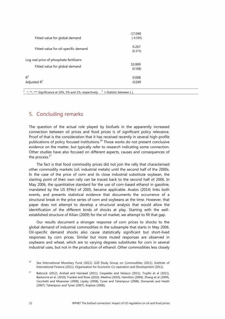
shocks and oil-specific demand shocks are significantly different from zero for nitrogens at 10% significance level, whereas only global shocks are significantly different from zero for phosphates. However Panel C, shows that none of the fitted values for nitrogens or phosphates are relevant in explaining the first difference of log real corn prices. This coincides with other findings in the literature that show a significant impact of the direct biofuel channel, but small and statistically insignificant relevance of the indirect input channels (eg transportation and fertilisers).25

25 See, for instance, Ciaian and Kancs (2011).

Analysis of fertilizer price data1,2

Sample 1974 - 2011 Table 2


Dependent variables

Log real price of nitrogen fertilisers Log real price of phosphate fertilisers

Panel A: Regressing fertilizer prices on oil prices (in log levels)

Constant 0.660*** [6.132]

0.488*** [3.956]

Log real oil price

0.461***

[6.909]

0.418***

[5.476]

R2 0.570

0.455

Panel B: Regressing fertilizer prices (in first difference) on structural shocks

Constant 0.006 [0.240]

0.007 [0.210]

Oil production

-0.013* [-1.693]

-0.006 [-0.576]

Global demand

0.023*** [3.375]

0.036***

[3.693]

Oil-specific demand

0.014* [1.953]

0.001 [0.118]

Corn

0.010 [1.275]

0.009 [0.809]

R2 0.414 0.325 Adjusted R2 0.341 0.241


Dependent variable: Log real corn prices

Panel C: Regressing corn prices on fitted values of fertilizer prices (in first difference)

Log real price of nitrogenized fertilizer:


5. Concluding remarks

The question of the actual role played by biofuels in the apparently increased connection between oil prices and food prices is of significant policy relevance. Proof of that is the consideration that it has received recently in several high-profile publications of policy focused institutions.26 Those works do not present conclusive evidence on the matter, but typically refer to research indicating some connection. Other studies have also focused on different aspects, causes and consequences of the process.27

The fact is that food commodity prices did not join the rally that characterised other commodity markets (oil, industrial metals) until the second half of the 2000s. In the case of the price of corn and its close industrial substitute soybean, the starting point of their own rally can be traced back to the second half of 2006. In May 2006, the quantitative standard for the use of corn-based ethanol in gasoline, mandated by the US EPAct of 2005, became applicable. Avalos (2014) links both events, and presents statistical evidence that documents the occurrence of a structural break in the price series of corn and soybeans at the time. However, that paper does not attempt to develop a structural analysis that would allow the identification of the different kinds of shocks at play. Starting with the well-established structure of Kilian (2009) for the oil market, we attempt to fill that gap.

Our results document a stronger response of corn prices to shocks to the global demand of industrial commodities in the subsample that starts in May 2006. Oil-specific demand shocks also cause statistically significant but short-lived responses by corn prices. Similar but more muted responses are observed in soybeans and wheat, which are to varying degrees substitutes for corn in several industrial uses, but not in the production of ethanol. Other commodities less closely

26 See International Monetary Fund (2012), G20 Study Group on Commodities (2011), Institute of

International Finance (2011), Organisation for Economic Co-operation and Development (2011). 27 Babcock (2012), Arshad and Hameed (2011), Cespedes and Velasco (2011), Trujillo et al (2011),

Bastourre et al. (2010), Frankel and Rose (2010), Medina (2010), Hamilton (2009), Zhang et al (2009), Cecchetti and Moessner (2008), Lipsky (2008), Tyner and Taheripour (2008), Domanski and Heath (2007), Taheripour and Tyner (2007), Koplow (2006),

Fitted value for global demand -17.040 [-0.595]

Fitted value for oil-specific demand 0.267 [0.373]

Log real price of phosphate fertilizers:

Fitted value for global demand 10.999 [0.588]

R2 0.008 Adjusted R2 -0.049

1 *, **, *** Significance at 10%, 5% and 1%, respectively. 2 t-Statistic between [ ].


or not at all related to US ethanol production, like sugar or cocoa, do not display similar responses. In further analyses we found that global liquidity had a significant impact on the structural shocks to the global demand for industrial commodities, and seems to have impacted oil and then food prices through that channel. Finally, we describe the alternative transmission channels between oil and corn markets that the literature proposes. Our test of the fertilizer cost channel is not supported by the data. Lack of data prevents us from testing the transportation cost channel, although it seems unlikely that such an idiosyncratic factor can have a large bearing on the pricing of a globally traded commodity like corn. That leaves ethanol as the main potential channel connecting both markets.

These results are of great practical relevance for producers of ethanol-related crops. As a consequence of stagnant gasoline demand in the US, in part resulting from the slow economic recovery after the Great Recession, the industry has been increasingly talking since 2012 about a “Blend Wall.” That is the inability of gasoline blenders to keep up with the increasing quantitative mandates of the law, just when they were becoming binding. To fulfil the mandates would have required the industry to move to gasoline blends with ethanol content much higher than the 10 percent that has been the standard so far. That would have required costly technical adjustments in distribution and storage facilities. The regulator responded by increasingly issuing ethanol waivers, which might explain the substantial depreciation of corn with respect to oil in recent months. Future price developments might depend significantly on the next regulatory steps.

References

Aasveit, K, H Bjørnland and L Thorsrud (2012): “What drives oil prices? Emerging versus developed economies”, Norges Bank Working Paper 2012/11.

Anzuini, A, MJ Lombardi and P Pagano (2013): “The impact of monetary policy shocks on commodity prices”, International Journal of Central Banking, 9, pp 119– 144.

Arshad, FM and Hameed AAA (2009): “The long run relationship between petroleum and cereals prices”, Global Economy and Finance Journal, 2, pp 91–100.

Avalos, F (2014): “Do oil prices drive food prices? The tale of a structural break”, Journal of International Money and Finance 42, pp 253-271.

Babcock, B (2012): “Updated assessment of the drought´s impacts on crop prices and biofuel production”, CARD Policy Briefs, August.

Banbura, M and M Modugno (2013), “Maximum likelihood estimation of factor models on datasets with arbitrary pattern of missing data”, Journal of Applied Econometrics, forthcoming.

Bastourre, D, J Carrera and J Ibarlucía (2010): “Commodity prices: structural factors, financial markets and non-linear dynamics”, BCRA Working Paper Series, 6, September.

Baumeister, C and L Kilian (2013): “Do oil price increases cause higher food prices?“, Bank of Canada Working Paper, 13-52.


Bernanke, BS and AS Blinder (1992): “The federal funds rate and the channels of monetary transmission”, American Economic Review, 82, pp 901–921.

Calvo, G (2008): “Exploding commodity prices, lax monetary policy, and sovereign wealth funds”, Vox, June.

Candelon, B and H Lütkepohl (2001): “On the reliability of Chow-type tests for parameter constancy in multivariate dynamic models”, Economic Letters, 73, pp 155–160.

Cecchetti, S and R Moessner (2008): “Commodity prices and inflation dynamics”, BIS Quarterly Review, December.

Céspedes, L and A Velasco (2011): “Was this time different?: Fiscal policy in commodity republics”, BIS Working Papers 365.

Ciaian P and d Kancs (2011): “Interdependencies in the energy-bioenergy-food price systems: A cointegration analysis”, Resource and Energy Economics 33, pp 326-348

Domanski, D and A Heath (2007): “Financial investors and commodity markets”, BIS Quarterly Review, March.

Eickmeier, S, L Gambacorta and B Hofmann (2013): “Understanding global liquidity”, BIS Working Paper, 402.

Elam, T (2013): “The RFS, fuel and food prices, and the need for reform”, FarmEcon LLC Papers, April.

Fattouh, B, L Kilian and L Mahadeva (2012): “The role of speculation in oil markets: what have we learned so far?”, CEPR Discussion Paper, 8916.

Frankel, J (2006): “The effect of monetary policy on real commodity prices,” NBER Working Paper, 12713.

Frankel, J and A Rose (2010): “Determinants of agricultural and mineral commodity prices”, Harvard Kennedy School Research Working Paper Series.

G20 Study Group on Commodities (2011): “Report of the G20 Study Group on commodities”, July.

Hamilton, J (2009): “Causes and consequences of the oil shock of 2007-08”, NBER Working Paper 15002.

Hausman, C, M Auffhammer and P Berck (2012): “Farm acreage shocks and crop prices: An SVAR approach to understanding the impacts of biofuels“, Environmental Resource Economics 53, pp 117-136.

Institute of International Finance (2011), “Financial investment in commodities markets: potential impact on commodity prices and volatility”, IIF Commodities Task Force Submission to the G20, September.

International Monetary Fund (2012): “Special feature: Commodity market review”, World Economic Outlook, October.

Koplow, D (2006): “Biofuels – At what cost? Government support for ethanol and biodiesel in the United States,” Global Subsidies Initiative, International Institute for Sustainable Development.

Lipsky, J (2008): “Commodity prices and global inflation”, remarks at the Council of Foreign Relations, May.


Lombardi, MJ and I Van Robays (2011): “Do financial investors destabilize the oil price?”, ECB Working Paper, 1346.

Lütkepohl, H (2005): “New Introduction to Multiple Time Series Analysis”, Springer.

Medina, L (2010): “The dynamic effects of commodity prices on fiscal performance in Latin America,” IMF Working Paper, 10/192.

Nazlioglu, S (2011): World oil and agricultural commodity prices: Evidence from nonlinear causality”, Energy Policy 39, pp 2935-2943.

Nazlioglu, S, C Erdem and U Soytas (2013): “Volatility spillover between oil and agricultural commodity markets”, Energy Economics 36, pp 658-665.

Organisation for Economic Co-operation and Development, and Food and Agriculture Organization (2011): “Agricultural outlook 2011-2020,” http://dx.doi.org/10.1787/agr_outlook-2011-en.

Pesaran, M and Y Shin (1998): “Generalized impulse response analysis in linear multivariate models”, Economic Letters, 58, pp 17–29.

Schnepf, R and B Yacobucci (2013): “Renewable Fuel Standard (RFS): Overview and issues”, CRS Report for Congress, March.

Trujillo-Barrera, A, M Mallory and P García (2011): “Volatility spillovers in the U.S. crude oil, corn, and ethanol markets”, Proceedings of the NCCC-134 Conference on Applied Commodity Price Analysis, Forecasting, and Market Risk Management.

Taheripour, F and W Tyner (2007): “Ethanol subsidies, who gets the benefits?”, Bio-fuels, Food and Feed Trade-offs Conference, April.

Tyner, W and F Taheripour (2008): “Policy options for integrated energy and agricultural markets”, Review of Agricultural Economics, 30, pp 387–396.

Peersman, G and I Van Robays (2010): “Oil and the euro area economy”, Economic Policy, 24, pp 603–651.

Yacobucci, B (2006): “Fuel ethanol: Background and public policy issues”, CRS Report for Congress, October.

Zhang, Z, L Lohr, C Escalante and M Wetzstein (2009): “Ethanol, corn, and soybean price relations in a volatile vehicle-fuels market”, Energies, 2, pp 320–339.

bis working papers · bis working papers no 487 ... many commentators started to speculate on...

Documents