bis working papers · bis working papers no 570 unconventional monetary policies: a re-appraisal by...
TRANSCRIPT
BIS Working PapersNo 570
Unconventional monetary policies: a re-appraisal by Claudio Borio and Anna Zabai
Monetary and Economic Department
July 2016
JEL classification: E40, E50, E52, E58, E60.
Keywords: unconventional monetary policies, balance sheet policies, forward guidance, negative interest rates.
BIS Working Papers are written by members of the Monetary and Economic Department of the Bank for International Settlements, and from time to time by other economists, and are published by the Bank. The papers are on subjects of topical interest and are technical in character. The views expressed in them are those of their authors and not necessarily the views of the BIS.
This publication is available on the BIS website (www.bis.org).
© Bank for International Settlements 2016. All rights reserved. Brief excerpts may be reproduced or translated provided the source is stated.
ISSN 1020-0959 (print) ISSN 1682-7678 (online)
WP570 Unconventional monetary policies: a re-appraisal i
Unconventional monetary policies: a re-appraisal
Claudio Borio and Anna Zabai#
Abstract
We explore the effectiveness and balance of benefits and costs of so-called “unconventional” monetary policy measures extensively implemented in the wake of the financial crisis: balance sheet policies (commonly termed “quantitative easing”), forward guidance and negative policy rates. Our objective is to provide the reader with a helpful entry point to the burgeoning empirical literature and with a specific perspective on the complex issues involved. We reach three main conclusions: there is ample evidence that, to varying degrees, these measures have succeeded in influencing financial conditions even though their ultimate impact on output and inflation is harder to pin down; the balance of the benefits and costs is likely to deteriorate over time; and the measures are generally best regarded as exceptional, for use in very specific circumstances. Whether this will turn out to be the case, however, is doubtful at best and depends on more fundamental features of monetary policy frameworks. In the paper, we also provide a critique of prevailing analyses of “helicopter money” and explore in more depth the role of negative nominal interest rates in our fundamentally monetary economies, highlighting some risks.
Keywords: unconventional monetary policies, balance sheet policies, forward guidance, negative interest rates.
JEL classification: E40, E50, E52, E58, E60.
# Bank for International Settlements.
This paper was prepared for R Lastra and P Conti-Brown (eds), Research Handbook on Central Banking, Edward Elgar Publishing Ltd. We thank Piti Disyatat, Dietrich Domanski and Hyun Shin for comments and suggestions. Jeff Slee and Anamaria Illes provided excellent statistical assistance. The views expressed in this paper are those of the authors and do not necessarily reflect those of the BIS.

WP570 Unconventional monetary policies: a re-appraisal iii
Contents
Abstract ......................................................................................................................................................... i
Introduction ............................................................................................................................................... 1
I. A taxonomy and a few facts ........................................................................................................ 2
Taxonomy .......................................................................................................................................... 2
What central banks have done ................................................................................................. 6
II. Influence on financial conditions: what do we know? ...................................................... 9
Balance sheet policies ................................................................................................................. 10
Forward guidance ........................................................................................................................ 14
Negative policy rates .................................................................................................................. 19
III. Influence on the macro-economy and broader considerations ................................. 21
Formal empirical evidence on output and inflation ....................................................... 22
The importance of context and measure-specific characteristics ............................. 24
Box 1: Delving into negative interest rates and “money illusion” .................... 27
Box 2: Understanding “helicopter money” ................................................................ 29
The political economy ................................................................................................................ 31
Conclusion ................................................................................................................................................ 34
References ................................................................................................................................................ 35

WP570 Unconventional monetary policies: a re-appraisal 1
Introduction
They were supposed to be exceptional and temporary – hence the term “unconventional”. They risk becoming standard and permanent, as the boundaries of the unconventional are stretched day after day.
Following the Great Financial Crisis, central banks in the major economies have adopted a whole range of new measures to influence monetary and financial conditions. The measures have gone far beyond the pre-crisis typical mode of operation – controlling a short-term policy rate and moving it within a positive range. To be sure, some of these measures had already been pioneered by the Bank of Japan roughly a decade earlier in the wake of that country’s banking crisis and stubbornly low inflation. But no one had anticipated that they would spread to the rest of the world so quickly and would become so daring.
How effective have these measures been? What broader issues do they raise? These are the two main questions we address in this essay. We do not intend to be comprehensive or provide a definitive analysis – the issues are far too complex and controversial. Rather, our objective is simply to take our cue from the burgeoning literature to provide some reflections on the subject. This should help the reader gain easier access to the rapidly growing body of work and approach it with one more perspective in mind.
What is “conventional” or not is partly in the eye of the beholder. To define our coverage, we take as benchmark pre-crisis implementation frameworks. On that basis, we discuss: (i) using the central bank’s balance sheet to influence financial conditions beyond the short-term rate – “balance sheet policies” (Borio and Disyatat (2010)); (ii) actively managing expectations of the future path of the policy rate to provide extra stimulus when rates have reached their (perceived) lower bound – (interest rate) “forward guidance”; and (iii) setting policy rates below zero in nominal terms – “negative interest rate policy “ (NIRP). We thus exclude from the analysis foreign exchange intervention although, analytically, it is a subset of balance sheet policies (Borio and Disyatat (2010)).1 In addition, we limit our discussion to four central banks – the Federal Reserve, the European Central Bank (ECB), the Bank of Japan and the Bank of England – except when we address NIRP, in which case we briefly touch on the experience of the Swiss National Bank (SNB), Danmarks Nationalbank and the Swedish Riksbank.
We highlight three conclusions.
First, there is ample evidence that, to varying degrees, these measures have succeeded in influencing financial conditions. There is little doubt that they have had a lasting impact on bond yields, various asset prices and exchange rates. Their relative effectiveness, however, is still subject to debate, as it is sometimes difficult to disentangle their impact (eg that of forward guidance from that of large-scale asset purchases). The same conclusion holds for their ultimate impact on output and inflation. Here, the empirical evidence is thinner and the researcher faces tougher
1 What is specific about foreign exchange intervention is (i) the asset purchased – denominated in
foreign rather than domestic currency – and, hence (ii) the aspect of financial conditions targeted – the exchange rate rather than a set of domestic asset prices. But foreign exchange intervention was already a standard policy tool pre-crisis around the world. At the same time, we do discuss briefly the use of foreign exchange swap lines, used to address funding conditions in foreign currency.
2 WP570 Unconventional monetary policies: a re-appraisal
challenges. These include difficulties in developing the correct metrics and in filtering out the influence of other factors on output and inflation (eg so-called “headwinds”) as well as the need to rely more heavily on modelling assumptions.
Second, formal econometric evidence on whether such policies are subject to diminishing returns is limited, partly owing to methodological complications. Views, therefore, differ. Our own assessment is that this is likely to be the case. There are bound to be limits to how far nominal interest rates can be reduced and risk spreads compressed. And there may be discontinuities and tipping points in the behaviour of financial intermediaries and economic agents more generally. Examples include the impact on the profitability and resilience of financial intermediaries and on the public’s confidence.
Finally, there are broader questions about the long-term effectiveness and desirability of these measures. Some have to do with the measures’ overall impact on the central bank goals; others with political economy considerations, which may ultimately undermine the central bank’s perceived legitimacy and autonomy (or “independence”). Exit issues loom large. Our view is that many of these measures should be best regarded as exceptional and for use in very specific circumstances, rather than be considered normal tools for normal conditions. Whether this will turn out to be the case, however, is doubtful at best and depends on more fundamental features of monetary policy frameworks.
The rest of the essay is organised as follows. Section I presents a taxonomy of central bank measures along the lines of Borio and Disyatat (2010) and then sketches what central banks have done. Section II briefly summarises and evaluates the evidence on the effectiveness of the various measures in influencing financial conditions. Section III examines their impact on output and inflation and addresses broader considerations, including the issues raised by exit and political economy considerations. The conclusions highlight key policy challenges in the years ahead. One box provides a critique of prevailing analyses of “helicopter money”; the other discusses in more depth the role of negative nominal interest rates in our fundamentally monetary economies, highlighting some risks.
I. A taxonomy and a few facts
Taxonomy
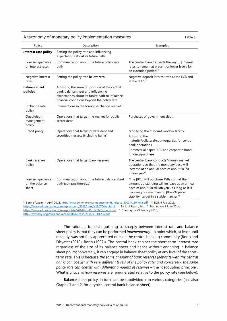
Monetary policy is implemented in two ways (Table 1). One is through interest rate policy, whereby the central bank influences financial conditions by setting, or closely controlling, a short-term rate (often overnight) and by steering expectations about where it will be set in future (“interest rate forward guidance”). The other is through balance sheet policy, whereby the central bank influences financial conditions beyond the short-term rate by adjusting its balance sheet (size and/or composition). Typical examples of balance sheet policy include large-scale asset purchases and the supply of central bank funding (“liquidity”) at non-standard terms and conditions (eg at long maturities, for specific lending purposes). Just as in the case of interest rate policy, the central bank may also wish to steer expectations about future balance sheet adjustments (“balance sheet forward guidance”).
WP570 Unconventional monetary policies: a re-appraisal 3
The rationale for distinguishing so sharply between interest rate and balance sheet policy is that they can be performed independently – a point which, at least until recently, was not fully appreciated outside the central banking community (Borio and Disyatat (2010), Borio (1997)). The central bank can set the short-term interest rate regardless of the size of its balance sheet and hence without engaging in balance sheet policy; conversely, it can engage in balance sheet policy at any level of the short-term rate. This is because the same amount of bank reserves (deposits with the central bank) can coexist with very different levels of the policy rate; and conversely, the same policy rate can coexist with different amounts of reserves – the “decoupling principle”. What is critical is how reserves are remunerated relative to the policy rate (see below).
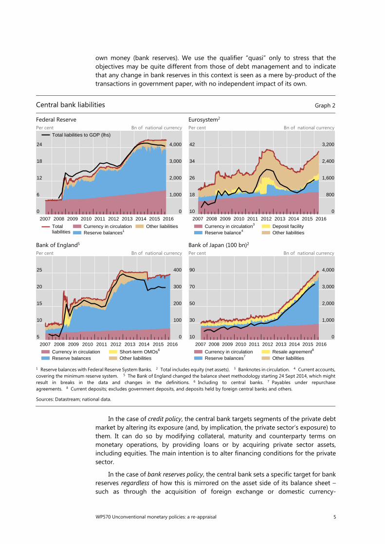
Balance sheet policy, in turn, can be subdivided into various categories (see also Graphs 1 and 2, for a typical central bank balance sheet).
A taxonomy of monetary policy implementation measures Table 1
Policy Description Examples
Interest rate policy Setting the policy rate and influencing expectations about its future path
Forward guidance on interest rates
Communication about the future policy rate path
The central bank “expects the key […] interest rates to remain at present or lower levels for an extended period”2
Negative interest rates
Setting the policy rate below zero Negative deposit interest rate at the ECB and at the BOJ4, 5
Balance sheet policies
Adjusting the size/composition of the central bank balance sheet and influencing expectations about its future path to influence financial conditions beyond the policy rate
Exchange rate policy
Interventions in the foreign exchange market
Quasi-debt management policy
Operations that target the market for public sector debt
Purchases of government debt
Credit policy Operations that target private debt and securities markets (including banks)
Modifying the discount window facility Adjusting the maturity/collateral/counterparties for central bank operations Commercial paper, ABS and corporate bond funding/purchase
Bank reserves policy
Operations that target bank reserves The central bank conducts “money market operations so that the monetary base will increase at an annual pace of about 60-70 trillion yen”1
Forward guidance on the balance sheet
Communication about the future balance sheet path (composition/size)
“The [BOJ] will purchase JGBs so that their amount outstanding will increase at an annual pace of about 50 trillion yen... as long as it is necessary for maintaining [the 2% price stability] target in a stable manner”3
1 Bank of Japan, 4 April 2013, http://www.boj.or.jp/en/announcements/release_2013/k130404a.pdf. 2 ECB, 4 July 2013, https://www.ecb.europa.eu/press/pressconf/2013/html/is130704.en.html. 3 Bank of Japan, ibid. 4 Starting on 5 June 2014, https://www.ecb.europa.eu/press/pr/date/2014/html/pr140605_3.en.html. 5 Starting on 29 January 2016, http://www.boj.or.jp/en/announcements/release_2016/k160129a.pdf.
4 WP570 Unconventional monetary policies: a re-appraisal
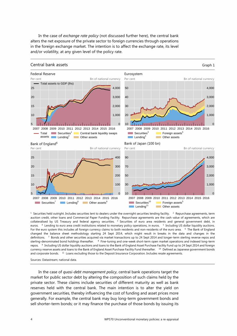
In the case of exchange rate policy (not discussed further here), the central bank alters the net exposure of the private sector to foreign currencies through operations in the foreign exchange market. The intention is to affect the exchange rate, its level and/or volatility, at any given level of the policy rate.
In the case of quasi-debt management policy, central bank operations target the market for public sector debt by altering the composition of such claims held by the private sector. These claims include securities of different maturity as well as bank reserves held with the central bank. The main intention is to alter the yield on government securities, thereby influencing the cost of funding and asset prices more generally. For example, the central bank may buy long-term government bonds and sell shorter-term bonds; or it may finance the purchase of those bonds by issuing its
Central bank assets Graph 1
Federal Reserve Eurosystem Per cent Bn of national currency Per cent Bn of national currency
Bank of England6 Bank of Japan (100 bn)Per cent Bn of national currency Per cent Bn of national currency
1 Securities held outright. Includes securities lent to dealers under the overnight securities lending facility. 2 Repurchase agreements, term auction credit, other loans and Commercial Paper Funding Facility. Repurchase agreements are the cash value of agreements, which are collateralised by US Treasury and federal agency securities. 3 Securities of euro area residents and general government debt, in euros. 4 Lending to euro area credit institutions related to monetary policy operations, in euros. 5 Including US dollar liquidity auctions.For the euro system this includes all foreign currency claims to both residents and non-residents of the euro area. 6 The Bank of England changed the balance sheet methodology starting 24 Sept 2014, which might result in breaks in the data and changes in thedefinitions. 7 Bonds and other securities acquired via market transactions up to 24 Sept 2014 and longer-term sterling reverse repos and sterling-denominated bond holdings thereafter. 8 Fine-tuning and one-week short-term open market operations and indexed long-term repos. 9 Including US dollar liquidity auctions and loans to the Bank of England Asset Purchase Facility Fund up to 24 Sept 2014 and foreign currency reserve assets and loans to the Bank of England Asset Purchase Facility Fund thereafter. 10 Defined as Japanese government bondsand corporate bonds. 11 Loans excluding those to the Deposit Insurance Corporation. Includes resale agreements.
Sources: Datastream; national data.
5
10
15
20
25
0
1,000
2,000
3,000
4,000
2007 2008 2009 2010 2011 2012 2013 2014 2015 2016
Total assets
Securities1
Lending2Central bank liquidity swapsOther assets
Total assets to GDP (lhs)
10
20
30
40
50
0
1,000
2,000
3,000
4,000
2007 2008 2009 2010 2011 2012 2013 2014 2015 2016
Securities3
Lending4Foreign assets5
Other assets
5
10
15
20
25
0
100
200
300
400
2007 2008 2009 2010 2011 2012 2013 2014 2015 2016
Securities7 Lending8 Other assets9
10
30
50
70
90
0
1,000
2,000
3,000
4,000
2007 2008 2009 2010 2011 2012 2013 2014 2015 2016
Securities10
Lending11Foreign assets5
Other assets
WP570 Unconventional monetary policies: a re-appraisal 5
own money (bank reserves). We use the qualifier “quasi” only to stress that the objectives may be quite different from those of debt management and to indicate that any change in bank reserves in this context is seen as a mere by-product of the transactions in government paper, with no independent impact of its own.
In the case of credit policy, the central bank targets segments of the private debt market by altering its exposure (and, by implication, the private sector’s exposure) to them. It can do so by modifying collateral, maturity and counterparty terms on monetary operations, by providing loans or by acquiring private sector assets, including equities. The main intention is to alter financing conditions for the private sector.
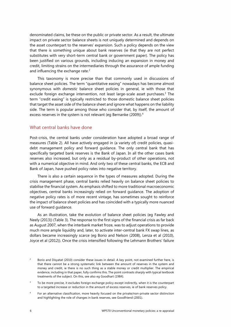
In the case of bank reserves policy, the central bank sets a specific target for bank reserves regardless of how this is mirrored on the asset side of its balance sheet – such as through the acquisition of foreign exchange or domestic currency-
Central bank liabilities Graph 2
Federal Reserve Eurosystem2 Per cent Bn of national currency Per cent Bn of national currency
Bank of England5 Bank of Japan (100 bn)2 Per cent Bn of national currency Per cent Bn of national currency
1 Reserve balances with Federal Reserve System Banks. 2 Total includes equity (net assets). 3 Banknotes in circulation. 4 Current accounts, covering the minimum reserve system. 5 The Bank of England changed the balance sheet methodology starting 24 Sept 2014, which mightresult in breaks in the data and changes in the definitions. 6 Including to central banks. 7 Payables under repurchase agreements. 8 Current deposits; excludes government deposits, and deposits held by foreign central banks and others.
Sources: Datastream; national data.
0
6
12
18
24
0
1,000
2,000
3,000
4,000
2007 2008 2009 2010 2011 2012 2013 2014 2015 2016
Total liabilities
Currency in circulationReserve balances1
Other liabilities
Total liabilities to GDP (lhs)
10
18
26
34
42
0
800
1,600
2,400
3,200
2007 2008 2009 2010 2011 2012 2013 2014 2015 2016
Currency in circulation3
Reserve balance4Deposit facilityOther liabilities
5
10
15
20
25
0
100
200
300
400
2007 2008 2009 2010 2011 2012 2013 2014 2015 2016
Currency in circulationReserve balances
Short-term OMOs6
Other liabilities
10
30
50
70
90
0
1,000
2,000
3,000
4,000
2007 2008 2009 2010 2011 2012 2013 2014 2015 2016
Currency in circulationReserve balances7
Resale agreement8
Other liabilities
6 WP570 Unconventional monetary policies: a re-appraisal
denominated claims, be these on the public or private sector. As a result, the ultimate impact on private sector balance sheets is not uniquely determined and depends on the asset counterpart to the reserves’ expansion. Such a policy depends on the view that there is something unique about bank reserves (ie that they are not perfect substitutes with very short-term central bank or government paper). The policy has been justified on various grounds, including inducing an expansion in money and credit, limiting strains on the intermediaries through the assurance of ample funding and influencing the exchange rate.2
This taxonomy is more precise than that commonly used in discussions of balance sheet policies. The term “quantitative easing” nowadays has become almost synonymous with domestic balance sheet policies in general, ie with those that exclude foreign exchange intervention, not least large-scale asset purchases.3 The term “credit easing” is typically restricted to those domestic balance sheet policies that target the asset side of the balance sheet and ignore what happens on the liability side. The term is popular among those who consider that, by itself, the amount of excess reserves in the system is not relevant (eg Bernanke (2009)).4
What central banks have done
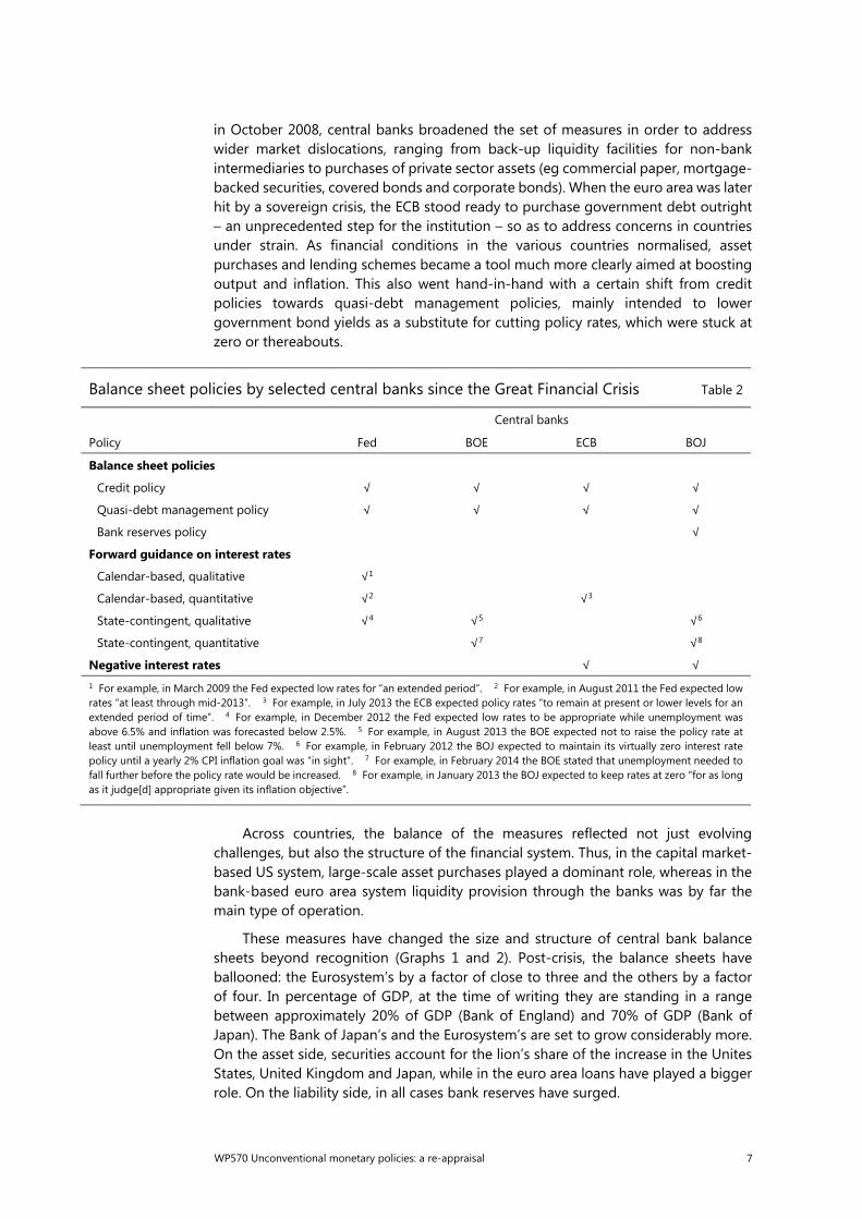
Post-crisis, the central banks under consideration have adopted a broad range of measures (Table 2). All have actively engaged in (a variety of) credit policies, quasi-debt management policy and forward guidance. The only central bank that has specifically targeted bank reserves is the Bank of Japan. In all the other cases bank reserves also increased, but only as a residual by-product of other operations, not with a numerical objective in mind. And only two of these central banks, the ECB and Bank of Japan, have pushed policy rates into negative territory.
There is also a certain sequence in the types of measures adopted. During the crisis management phase, central banks relied heavily on balance sheet policies to stabilise the financial system. As emphasis shifted to more traditional macroeconomic objectives, central banks increasingly relied on forward guidance. The adoption of negative policy rates is of more recent vintage, has sometimes sought to reinforce the impact of balance sheet policies and has coincided with a typically more nuanced use of forward guidance.
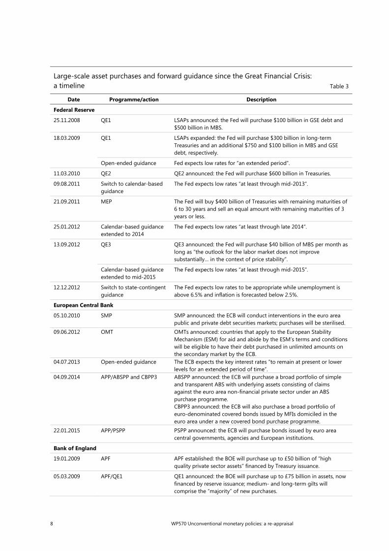
As an illustration, take the evolution of balance sheet policies (eg Fawley and Neely (2013)) (Table 3). The response to the first signs of the financial crisis as far back as August 2007, when the interbank market froze, was to adjust operations to provide much more ample liquidity and, later, to activate inter-central bank FX swap lines, as dollars became increasingly scarce (eg Borio and Nelson (2008), Lenza et al (2010), Joyce et al (2012)). Once the crisis intensified following the Lehmann Brothers’ failure
2 Borio and Disyatat (2010) consider these issues in detail. A key point, not examined further here, is
that there cannot be a strong systematic link between the amount of reserves in the system and money and credit, ie there is no such thing as a stable money or credit multiplier. The empirical evidence, including in that paper, fully confirms this. The point contrasts sharply with typical textbook treatments of the subject. On this, see also eg Goodhart (1984).
3 To be more precise, it excludes foreign exchange policy except indirectly, when it is the counterpart to a targeted increase or reduction in the amount of excess reserves, ie of bank reserves policy.
4 For an alternative classification, more heavily focused on the private/non-private sector distinction and highlighting the role of changes in bank reserves, see Goodfriend (2001).
WP570 Unconventional monetary policies: a re-appraisal 7
in October 2008, central banks broadened the set of measures in order to address wider market dislocations, ranging from back-up liquidity facilities for non-bank intermediaries to purchases of private sector assets (eg commercial paper, mortgage-backed securities, covered bonds and corporate bonds). When the euro area was later hit by a sovereign crisis, the ECB stood ready to purchase government debt outright – an unprecedented step for the institution – so as to address concerns in countries under strain. As financial conditions in the various countries normalised, asset purchases and lending schemes became a tool much more clearly aimed at boosting output and inflation. This also went hand-in-hand with a certain shift from credit policies towards quasi-debt management policies, mainly intended to lower government bond yields as a substitute for cutting policy rates, which were stuck at zero or thereabouts.
Across countries, the balance of the measures reflected not just evolving challenges, but also the structure of the financial system. Thus, in the capital market-based US system, large-scale asset purchases played a dominant role, whereas in the bank-based euro area system liquidity provision through the banks was by far the main type of operation.
These measures have changed the size and structure of central bank balance sheets beyond recognition (Graphs 1 and 2). Post-crisis, the balance sheets have ballooned: the Eurosystem’s by a factor of close to three and the others by a factor of four. In percentage of GDP, at the time of writing they are standing in a range between approximately 20% of GDP (Bank of England) and 70% of GDP (Bank of Japan). The Bank of Japan’s and the Eurosystem’s are set to grow considerably more. On the asset side, securities account for the lion’s share of the increase in the Unites States, United Kingdom and Japan, while in the euro area loans have played a bigger role. On the liability side, in all cases bank reserves have surged.
Balance sheet policies by selected central banks since the Great Financial Crisis Table 2
Policy
Central banks
Fed BOE ECB BOJ
Balance sheet policies
Credit policy √ √ √ √
Quasi-debt management policy √ √ √ √
Bank reserves policy √
Forward guidance on interest rates
Calendar-based, qualitative √1
Calendar-based, quantitative √2 √3
State-contingent, qualitative √4 √5 √6
State-contingent, quantitative √7 √8
Negative interest rates √ √ 1 For example, in March 2009 the Fed expected low rates for “an extended period”. 2 For example, in August 2011 the Fed expected low rates “at least through mid-2013”. 3 For example, in July 2013 the ECB expected policy rates “to remain at present or lower levels for an extended period of time”. 4 For example, in December 2012 the Fed expected low rates to be appropriate while unemployment was above 6.5% and inflation was forecasted below 2.5%. 5 For example, in August 2013 the BOE expected not to raise the policy rate at least until unemployment fell below 7%. 6 For example, in February 2012 the BOJ expected to maintain its virtually zero interest rate policy until a yearly 2% CPI inflation goal was “in sight”. 7 For example, in February 2014 the BOE stated that unemployment needed to fall further before the policy rate would be increased. 8 For example, in January 2013 the BOJ expected to keep rates at zero “for as long as it judge[d] appropriate given its inflation objective”.
8 WP570 Unconventional monetary policies: a re-appraisal
Large-scale asset purchases and forward guidance since the Great Financial Crisis: a timeline Table 3
Date Programme/action Description
Federal Reserve
25.11.2008 QE1 LSAPs announced: the Fed will purchase $100 billion in GSE debt and $500 billion in MBS.
18.03.2009 QE1 LSAPs expanded: the Fed will purchase $300 billion in long-term Treasuries and an additional $750 and $100 billion in MBS and GSE debt, respectively.
Open-ended guidance Fed expects low rates for “an extended period”.
11.03.2010 QE2 QE2 announced: the Fed will purchase $600 billion in Treasuries.
09.08.2011 Switch to calendar-based guidance
The Fed expects low rates “at least through mid-2013”.
21.09.2011 MEP The Fed will buy $400 billion of Treasuries with remaining maturities of 6 to 30 years and sell an equal amount with remaining maturities of 3 years or less.
25.01.2012 Calendar-based guidance extended to 2014
The Fed expects low rates “at least through late 2014”.
13.09.2012 QE3 QE3 announced: the Fed will purchase $40 billion of MBS per month as long as “the outlook for the labor market does not improve substantially… in the context of price stability”.
Calendar-based guidance extended to mid-2015
The Fed expects low rates “at least through mid-2015”.
12.12.2012 Switch to state-contingent guidance
The Fed expects low rates to be appropriate while unemployment is above 6.5% and inflation is forecasted below 2.5%.
European Central Bank
05.10.2010 SMP SMP announced: the ECB will conduct interventions in the euro area public and private debt securities markets; purchases will be sterilised.
09.06.2012 OMT OMTs announced: countries that apply to the European StabilityMechanism (ESM) for aid and abide by the ESM’s terms and conditions will be eligible to have their debt purchased in unlimited amounts on the secondary market by the ECB.
04.07.2013 Open-ended guidance The ECB expects the key interest rates “to remain at present or lower levels for an extended period of time”.
04.09.2014 APP/ABSPP and CBPP3 ABSPP announced: the ECB will purchase a broad portfolio of simple and transparent ABS with underlying assets consisting of claims against the euro area non-financial private sector under an ABS purchase programme. CBPP3 announced: the ECB will also purchase a broad portfolio of euro-denominated covered bonds issued by MFIs domiciled in the euro area under a new covered bond purchase programme.
22.01.2015 APP/PSPP PSPP announced: the ECB will purchase bonds issued by euro area central governments, agencies and European institutions.
Bank of England
19.01.2009 APF APF established: the BOE will purchase up to £50 billion of “high quality private sector assets” financed by Treasury issuance.
05.03.2009 APF/QE1 QE1 announced: the BOE will purchase up to £75 billion in assets, now financed by reserve issuance; medium- and long-term gilts will comprise the “majority” of new purchases.
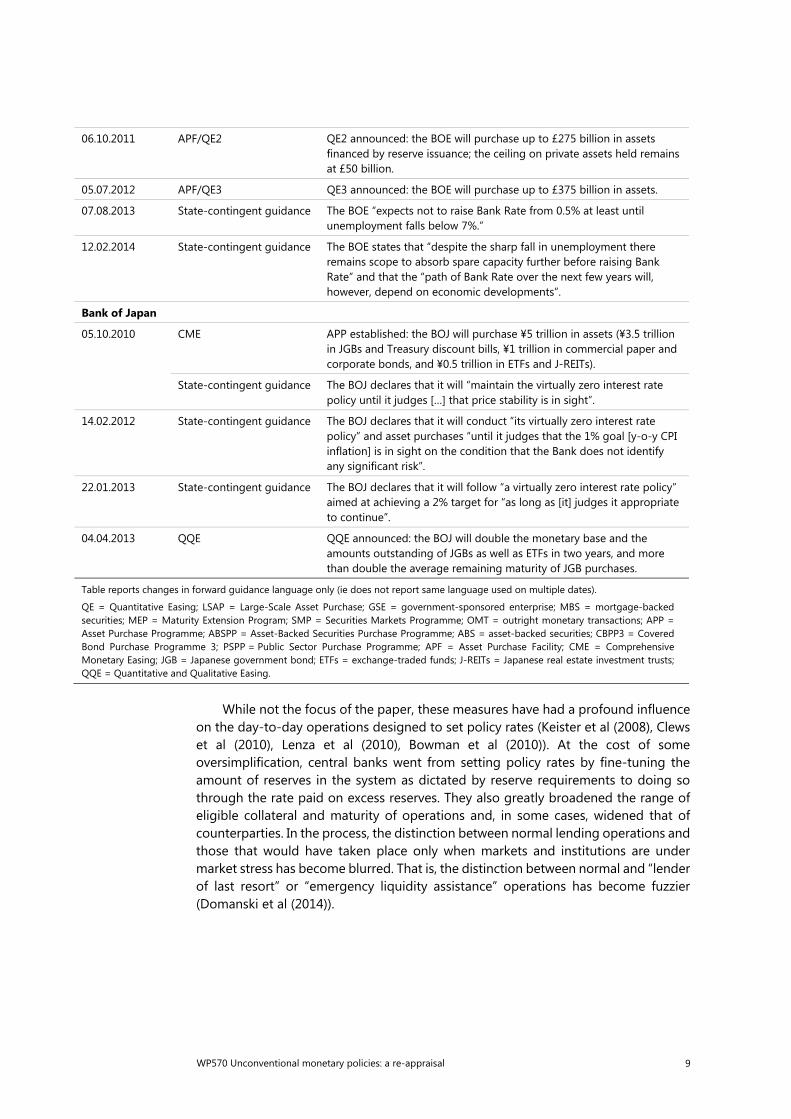
WP570 Unconventional monetary policies: a re-appraisal 9
While not the focus of the paper, these measures have had a profound influence on the day-to-day operations designed to set policy rates (Keister et al (2008), Clews et al (2010), Lenza et al (2010), Bowman et al (2010)). At the cost of some oversimplification, central banks went from setting policy rates by fine-tuning the amount of reserves in the system as dictated by reserve requirements to doing so through the rate paid on excess reserves. They also greatly broadened the range of eligible collateral and maturity of operations and, in some cases, widened that of counterparties. In the process, the distinction between normal lending operations and those that would have taken place only when markets and institutions are under market stress has become blurred. That is, the distinction between normal and “lender of last resort” or “emergency liquidity assistance” operations has become fuzzier (Domanski et al (2014)).
06.10.2011 APF/QE2 QE2 announced: the BOE will purchase up to £275 billion in assets financed by reserve issuance; the ceiling on private assets held remains at £50 billion.
05.07.2012 APF/QE3 QE3 announced: the BOE will purchase up to £375 billion in assets.
07.08.2013 State-contingent guidance The BOE “expects not to raise Bank Rate from 0.5% at least until unemployment falls below 7%.”
12.02.2014 State-contingent guidance The BOE states that “despite the sharp fall in unemployment there remains scope to absorb spare capacity further before raising Bank Rate” and that the “path of Bank Rate over the next few years will, however, depend on economic developments”.
Bank of Japan
05.10.2010 CME APP established: the BOJ will purchase ¥5 trillion in assets (¥3.5 trillion in JGBs and Treasury discount bills, ¥1 trillion in commercial paper and corporate bonds, and ¥0.5 trillion in ETFs and J-REITs).
State-contingent guidance The BOJ declares that it will “maintain the virtually zero interest rate policy until it judges […] that price stability is in sight”.
14.02.2012 State-contingent guidance The BOJ declares that it will conduct “its virtually zero interest rate policy” and asset purchases “until it judges that the 1% goal [y-o-y CPI inflation] is in sight on the condition that the Bank does not identify any significant risk”.
22.01.2013 State-contingent guidance The BOJ declares that it will follow “a virtually zero interest rate policy” aimed at achieving a 2% target for “as long as [it] judges it appropriate to continue”.
04.04.2013 QQE QQE announced: the BOJ will double the monetary base and the amounts outstanding of JGBs as well as ETFs in two years, and more than double the average remaining maturity of JGB purchases.
Table reports changes in forward guidance language only (ie does not report same language used on multiple dates).
QE = Quantitative Easing; LSAP = Large-Scale Asset Purchase; GSE = government-sponsored enterprise; MBS = mortgage-backed securities; MEP = Maturity Extension Program; SMP = Securities Markets Programme; OMT = outright monetary transactions; APP = Asset Purchase Programme; ABSPP = Asset-Backed Securities Purchase Programme; ABS = asset-backed securities; CBPP3 = Covered Bond Purchase Programme 3; PSPP = Public Sector Purchase Programme; APF = Asset Purchase Facility; CME = Comprehensive Monetary Easing; JGB = Japanese government bond; ETFs = exchange-traded funds; J-REITs = Japanese real estate investment trusts; QQE = Quantitative and Qualitative Easing.
10 WP570 Unconventional monetary policies: a re-appraisal
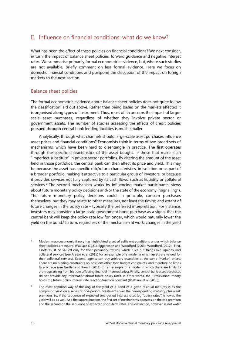
II. Influence on financial conditions: what do we know?
What has been the effect of these policies on financial conditions? We next consider, in turn, the impact of balance sheet policies, forward guidance and negative interest rates. We summarise primarily formal econometric evidence, but, where such studies are not available, briefly comment on less formal evidence. Here we focus on domestic financial conditions and postpone the discussion of the impact on foreign markets to the next section.
Balance sheet policies
The formal econometric evidence about balance sheet policies does not quite follow the classification laid out above. Rather than being based on the markets affected it is organised along types of instrument. Thus, most of it concerns the impact of large-scale asset purchases, regardless of whether they involve private sector or government assets. The number of studies assessing the effects of credit policies pursued through central bank lending facilities is much smaller.
Analytically, through what channels should large-scale asset purchases influence asset prices and financial conditions? Economists think in terms of two broad sets of mechanisms, which have been hard to disentangle in practice. The first operates through the specific characteristics of the asset bought, ie those that make it an “imperfect substitute” in private sector portfolios. By altering the amount of the asset held in those portfolios, the central bank can then affect its price and yield. This may be because the asset has specific risk/return characteristics, in isolation or as part of a broader portfolio, making it attractive to a particular group of investors, or because it provides services not fully captured by its cash flows, such as liquidity or collateral services.5 The second mechanism works by influencing market participants’ views about future monetary policy decisions and/or the state of the economy (“signalling”). The future monetary policy decisions could, in principle, concern purchases themselves, but they may relate to other measures, not least the timing and extent of future changes in the policy rate – typically the preferred interpretation. For instance, investors may consider a large-scale government bond purchase as a signal that the central bank will keep the policy rate low for longer, which would naturally lower the yield on the bond.6 In turn, regardless of the mechanism at work, changes in the yield
5 Modern macroeconomic theory has highlighted a set of sufficient conditions under which balance
sheet policies are neutral (Wallace (1981), Eggertsson and Woodford (2003), Woodford (2012)). First, assets must be valued only for their pecuniary returns, which rules out things like liquidity and collateral services (see Araújo et al (2015) for an example of a model in which assets are valued for their collateral services). Second, agents can buy arbitrary quantities at the same (market) prices. There are no binding constraints on positions other than budget constraints, and therefore no limits to arbitrage (see Gertler and Karadi (2011) for an example of a model in which there are limits to arbitrage arising from frictions affecting financial intermediaries). Finally, central bank asset purchases do not provide any information about future policy rates. In other words, the “`irrelevance'' theory holds the future policy interest rate reaction function constant (Bhattarai et al (2015)).
6 The most common way of thinking of the yield of a bond of a given residual maturity is as the compound yield on a series of one-period investments over the corresponding maturity plus a risk premium. So, if the sequence of expected one-period interest rates (eg ”policy rates”) is lower, the yield will be as well. As a first approximation, the first set of mechanisms operates on the risk premium and the second on the sequence of expected short-term rates. This distinction, however, is not water
WP570 Unconventional monetary policies: a re-appraisal 11
Impact of balance sheet policies on domestic yields and the exchange rate Table 4
Study Method Estimates
∆ 10-year Treasury yield (bp)
∆ 30-year MBS yield (bp)
∆ FX (%)
United States
QE1 – $1.75 trillion MBS; $300 billion Treasuries; $172 billion agency securities
Krishnamurthy and Vissing-Jorgensen (2011)
Event study –1071a –1071b
Gagnon et al (2011) Event study –912a –1132b
Hancock and Passmore (2011)
Time series regressions –443c
Christensen and Rudebusch (2012)
Event study, affine no-arbitrage model of the term structure
–894a
(–60,–33,–7)
D’Amico and King (2013) Cross-section regression –305a
D’Amico et al (2012) Time series regression –356a
(66,34)
Bauer and Rudebusch (2014)
Affine no-arbitrage model of the term structure
–897a
(38,62)
Neely (2015) Event study –948a –5.988c
Chadha et al (2016) Time-series regression –90 to –1159a
QE2 – $600 billion Treasuries MEP – $667 billion long-term Treasuries purchased; $667 billion short-term Treasuries sold
Krishnamurthy and Vissing-Jorgensen (2011)
Event study –3010a
–810b
Swanson (2011) Event study –1611a
Hamilton et al (2012) Time series regression –2212a D’Amico et al (2012) Time series regression –4513a
(78,22)
All programmes (includes QE3, $823 billion MBS; $790 billion Treasuries)
Swanson (2015) Time series regression –7.4614a –0.2614c
United Kingdom
QE – £375 billion gilts
∆ gilts yield (bp) ∆ FX (%)
Joyce et al (2011) Event study –100bp15a (10,90)
–415c
Joyce and Tong (2012) Event study, time series regressions
–97.616a
(2.5)
Christensen and Rudebusch (2012)
Event study, affine no–arbitrage model of the term structure
–4317a
(47,–135,–12)
McLaren et al (2014) Event study –9318a
(52)
tight: for instance, if the central bank painted a bleak picture of the economy, this could depress participants’ willingness to take on risk. For a discussion of this and related issues, see also Bauer and Rudebusch (2014).
12 WP570 Unconventional monetary policies: a re-appraisal
of the asset in question will ripple through the system, as they encourage further portfolio adjustments. For instance, if the yield on government bonds falls, yield-hungry investors may be induced to shift into riskier assets – an aspect of the so-called “risk-taking channel”.7,8
7 For an introduction to the risk-taking channel, see Borio and Zhu (2012); for further elaboration or
examples, see, in particular, Rajan (2005); for its operation in the context of exchange rates, see Shin (2012)).
8 Central banks have indeed used variations on these arguments to rationalise their actions. For instance, the Bank of England has argued that by pushing up the price of sovereign bonds, asset purchases drive investors into riskier securities, further compressing yields.
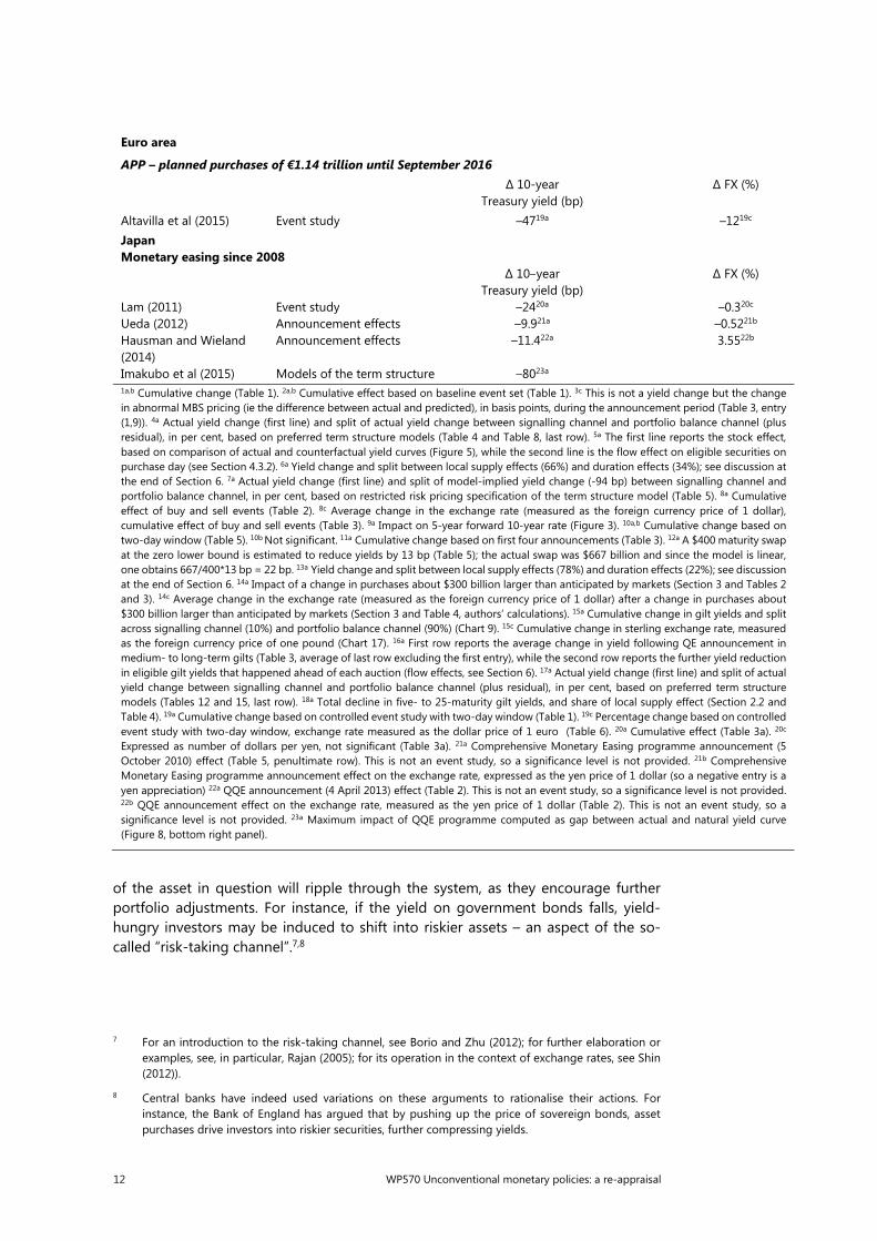
Euro area
APP – planned purchases of €1.14 trillion until September 2016 ∆ 10-year
Treasury yield (bp) ∆ FX (%)
Altavilla et al (2015) Event study –4719a –1219c Japan Monetary easing since 2008 ∆ 10–year
Treasury yield (bp) ∆ FX (%)
Lam (2011) Event study –2420a –0.320c
Ueda (2012) Announcement effects –9.921a –0.5221b
Hausman and Wieland (2014)
Announcement effects –11.422a 3.5522b
Imakubo et al (2015) Models of the term structure –8023a
1a,b Cumulative change (Table 1). 2a,b Cumulative effect based on baseline event set (Table 1). 3c This is not a yield change but the change in abnormal MBS pricing (ie the difference between actual and predicted), in basis points, during the announcement period (Table 3, entry (1,9)). 4a Actual yield change (first line) and split of actual yield change between signalling channel and portfolio balance channel (plus residual), in per cent, based on preferred term structure models (Table 4 and Table 8, last row). 5a The first line reports the stock effect, based on comparison of actual and counterfactual yield curves (Figure 5), while the second line is the flow effect on eligible securities on purchase day (see Section 4.3.2). 6a Yield change and split between local supply effects (66%) and duration effects (34%); see discussion at the end of Section 6. 7a Actual yield change (first line) and split of model-implied yield change (-94 bp) between signalling channel and portfolio balance channel, in per cent, based on restricted risk pricing specification of the term structure model (Table 5). 8a Cumulative effect of buy and sell events (Table 2). 8c Average change in the exchange rate (measured as the foreign currency price of 1 dollar), cumulative effect of buy and sell events (Table 3). 9a Impact on 5-year forward 10-year rate (Figure 3). 10a,b Cumulative change based on two-day window (Table 5). 10b Not significant. 11a Cumulative change based on first four announcements (Table 3). 12a A $400 maturity swap at the zero lower bound is estimated to reduce yields by 13 bp (Table 5); the actual swap was $667 billion and since the model is linear, one obtains 667/400*13 bp = 22 bp. 13a Yield change and split between local supply effects (78%) and duration effects (22%); see discussion at the end of Section 6. 14a Impact of a change in purchases about $300 billion larger than anticipated by markets (Section 3 and Tables 2 and 3). 14c Average change in the exchange rate (measured as the foreign currency price of 1 dollar) after a change in purchases about $300 billion larger than anticipated by markets (Section 3 and Table 4, authors’ calculations). 15a Cumulative change in gilt yields and split across signalling channel (10%) and portfolio balance channel (90%) (Chart 9). 15c Cumulative change in sterling exchange rate, measured as the foreign currency price of one pound (Chart 17). 16a First row reports the average change in yield following QE announcement in medium- to long-term gilts (Table 3, average of last row excluding the first entry), while the second row reports the further yield reduction in eligible gilt yields that happened ahead of each auction (flow effects, see Section 6). 17a Actual yield change (first line) and split of actual yield change between signalling channel and portfolio balance channel (plus residual), in per cent, based on preferred term structure models (Tables 12 and 15, last row). 18a Total decline in five- to 25-maturity gilt yields, and share of local supply effect (Section 2.2 and Table 4). 19a Cumulative change based on controlled event study with two-day window (Table 1). 19c Percentage change based on controlled event study with two-day window, exchange rate measured as the dollar price of 1 euro (Table 6). 20a Cumulative effect (Table 3a). 20c Expressed as number of dollars per yen, not significant (Table 3a). 21a Comprehensive Monetary Easing programme announcement (5 October 2010) effect (Table 5, penultimate row). This is not an event study, so a significance level is not provided. 21b Comprehensive Monetary Easing programme announcement effect on the exchange rate, expressed as the yen price of 1 dollar (so a negative entry is a yen appreciation) 22a QQE announcement (4 April 2013) effect (Table 2). This is not an event study, so a significance level is not provided. 22b QQE announcement effect on the exchange rate, measured as the yen price of 1 dollar (Table 2). This is not an event study, so a significance level is not provided. 23a Maximum impact of QQE programme computed as gap between actual and natural yield curve (Figure 8, bottom right panel).
WP570 Unconventional monetary policies: a re-appraisal 13
The empirical evidence follows a variety of approaches. The most common one consists of examining the behaviour of the relevant asset prices (or yields) around the policy announcement – “event analysis”. Ideally, one seeks to identify the “surprise” element, since the presumption is that markets only react to what they have not expected, ie to what is not already priced in. The second is to link directly through econometric methods the size and composition of the central banks’ balance sheets or other indicators of the operations to the behaviour of asset prices and returns. Event analysis is probably the more reliable approach, as it better identifies the source of the market reaction. The disadvantage is that the window over which the change is examined has to be rather small – typically ranging from minutes to at most a few days – to avoid including the impact of other factors.9 In addition, some studies seek to decompose the change into the risk (or term) premium and a measure of the expected path of future interest rates.
A look at the studies points to a number of findings (Table 4).
First, there is general agreement that large-scale asset purchases did have sizeable effects on financial conditions. This is true regardless of the assets purchased – eg government bonds or mortgage-backed securities – and of the financial prices considered – those of the assets purchased or others, such as equities and the exchange rate. Because of the different types of programmes and the methodologies used, it is very hard to provide a simple guide to the size of the effects. But, say, the cumulative impact of the Fed programmes on 10-year government bond yields may have been of the order of over -100 basis points.10
Second, most of the impact appears to take place on announcement, rather than once the purchases are actually executed. This is consistent with the view that markets are forward-looking, pricing actions once they are expected.
Third, the studies have a hard time distinguishing between the impact on the risk premium and on the expected path of future policy rates. Authors differ in their interpretation. This is hardly surprising, given the nature of the problem. Most probably, both mechanisms are at work.
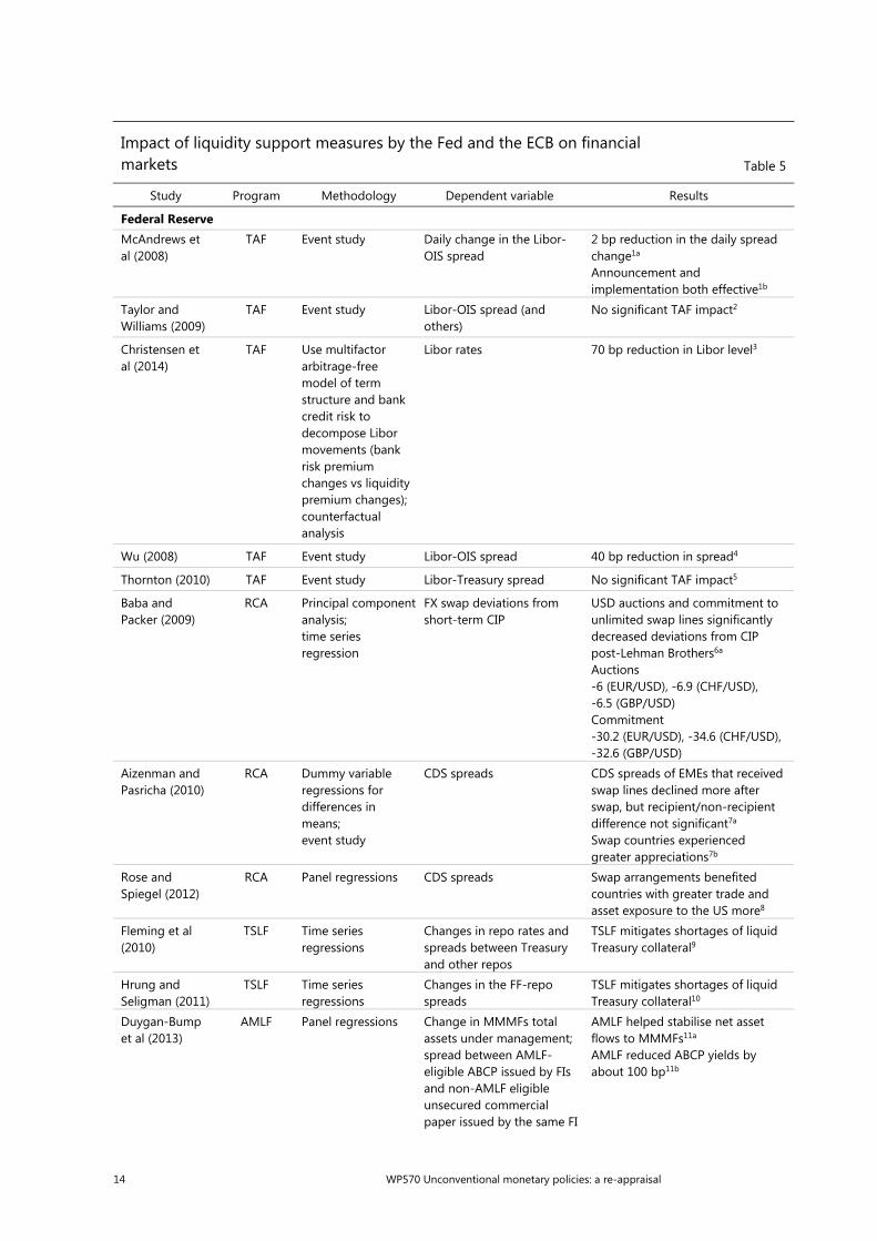
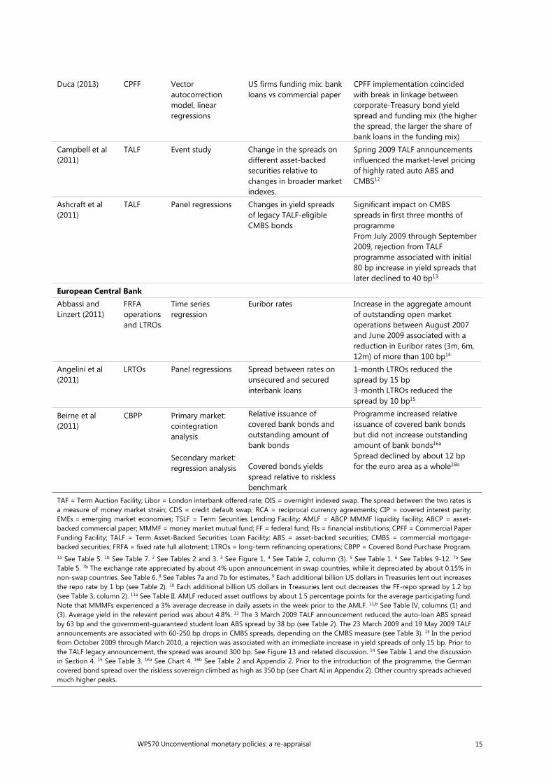
The literature on the impact of credit policies implemented through lending facilities is smaller. That said, certain preliminary conclusions seem reasonable (Table 5). In particular, the measures appear to have helped alleviate liquidity shortages in financial markets. Summarising the Federal Reserve experience, for example, Fleming (2012) argues that these measures improved market functioning while adhering to the general principle of lending against collateral at a penalty rate. The evidence about unconventional policy actions implemented by the ECB also suggests that they helped relieve stress in money markets and ease credit conditions more generally.
9 Combinations of the two methods are also possible, by including the (surprise element of) an
announcement in dynamic econometric relationships.
10 Consider the estimates in Table 4. Averaging the effects of QE1 across studies, we obtain about -76 basis points. Doing the same for QE2 and (the more limited evidence) for QE3 we get -28 and -7 basis points, respectively. This amounts to -112 in total.
14 WP570 Unconventional monetary policies: a re-appraisal
Impact of liquidity support measures by the Fed and the ECB on financial markets Table 5
Study Program Methodology Dependent variable Results
Federal Reserve McAndrews et al (2008)
TAF Event study Daily change in the Libor-OIS spread
2 bp reduction in the daily spread change1a
Announcement and implementation both effective1b
Taylor and Williams (2009)
TAF Event study Libor-OIS spread (and others)
No significant TAF impact2
Christensen et al (2014)
TAF Use multifactor arbitrage-free model of term structure and bank credit risk to decompose Libor movements (bank risk premium changes vs liquidity premium changes); counterfactual analysis
Libor rates 70 bp reduction in Libor level3
Wu (2008) TAF Event study Libor-OIS spread 40 bp reduction in spread4
Thornton (2010) TAF Event study Libor-Treasury spread No significant TAF impact5
Baba and Packer (2009)
RCA Principal component analysis; time series regression
FX swap deviations from short-term CIP
USD auctions and commitment to unlimited swap lines significantly decreased deviations from CIP post-Lehman Brothers6a Auctions -6 (EUR/USD), -6.9 (CHF/USD), -6.5 (GBP/USD) Commitment -30.2 (EUR/USD), -34.6 (CHF/USD), -32.6 (GBP/USD)
Aizenman and Pasricha (2010)
RCA Dummy variable regressions for differences in means; event study
CDS spreads CDS spreads of EMEs that received swap lines declined more after swap, but recipient/non-recipient difference not significant7a
Swap countries experienced greater appreciations7b
Rose and Spiegel (2012)
RCA Panel regressions CDS spreads Swap arrangements benefited countries with greater trade and asset exposure to the US more8
Fleming et al (2010)
TSLF Time series regressions
Changes in repo rates and spreads between Treasury and other repos
TSLF mitigates shortages of liquid Treasury collateral9
Hrung and Seligman (2011)
TSLF Time series regressions
Changes in the FF-repo spreads
TSLF mitigates shortages of liquid Treasury collateral10
Duygan-Bump et al (2013)
AMLF Panel regressions
Change in MMMFs total assets under management; spread between AMLF- eligible ABCP issued by FIs and non-AMLF eligible unsecured commercial paper issued by the same FI
AMLF helped stabilise net asset flows to MMMFs11a AMLF reduced ABCP yields by about 100 bp11b
WP570 Unconventional monetary policies: a re-appraisal 15
Duca (2013) CPFF Vector autocorrection model, linear regressions
US firms funding mix: bank loans vs commercial paper
CPFF implementation coincided with break in linkage between corporate-Treasury bond yield spread and funding mix (the higher the spread, the larger the share of bank loans in the funding mix)
Campbell et al (2011)
TALF Event study Change in the spreads on different asset-backed securities relative to changes in broader market indexes.
Spring 2009 TALF announcements influenced the market-level pricing of highly rated auto ABS and CMBS12
Ashcraft et al (2011)
TALF Panel regressions Changes in yield spreads of legacy TALF-eligible CMBS bonds
Significant impact on CMBS spreads in first three months of programme From July 2009 through September 2009, rejection from TALF programme associated with initial 80 bp increase in yield spreads that later declined to 40 bp13
European Central Bank Abbassi and Linzert (2011)
FRFA operations and LTROs
Time series regression
Euribor rates Increase in the aggregate amount of outstanding open market operations between August 2007 and June 2009 associated with a reduction in Euribor rates (3m, 6m, 12m) of more than 100 bp14
Angelini et al (2011)
LRTOs Panel regressions Spread between rates on unsecured and secured interbank loans
1-month LTROs reduced the spread by 15 bp 3-month LTROs reduced the spread by 10 bp15
Beirne et al (2011)
CBPP Primary market: cointegration analysis Secondary market: regression analysis
Relative issuance of covered bank bonds and outstanding amount of bank bonds Covered bonds yields spread relative to riskless benchmark
Programme increased relative issuance of covered bank bonds but did not increase outstanding amount of bank bonds16a Spread declined by about 12 bp for the euro area as a whole16b
TAF = Term Auction Facility; Libor = London interbank offered rate; OIS = overnight indexed swap. The spread between the two rates is a measure of money market strain; CDS = credit default swap; RCA = reciprocal currency agreements; CIP = covered interest parity; EMEs = emerging market economies; TSLF = Term Securities Lending Facility; AMLF = ABCP MMMF liquidity facility; ABCP = asset-backed commercial paper; MMMF = money market mutual fund; FF = federal fund; FIs = financial institutions; CPFF = Commercial Paper Funding Facility; TALF = Term Asset-Backed Securities Loan Facility; ABS = asset-backed securities; CMBS = commercial mortgage-backed securities; FRFA = fixed rate full allotment; LTROs = long-term refinancing operations; CBPP = Covered Bond Purchase Program. 1a See Table 5. 1b See Table 7. 2 See Tables 2 and 3. 3 See Figure 1. 4 See Table 2, column (3). 5 See Table 1. 6 See Tables 9-12. 7a See Table 5. 7b The exchange rate appreciated by about 4% upon announcement in swap countries, while it depreciated by about 0.15% in non-swap countries. See Table 6. 8 See Tables 7a and 7b for estimates. 9 Each additional billion US dollars in Treasuries lent out increases the repo rate by 1 bp (see Table 2). 10 Each additional billion US dollars in Treasuries lent out decreases the FF-repo spread by 1.2 bp (see Table 3, column 2). 11a See Table II. AMLF reduced asset outflows by about 1.5 percentage points for the average participating fund. Note that MMMFs experienced a 3% average decrease in daily assets in the week prior to the AMLF. 11,b See Table IV, columns (1) and (3). Average yield in the relevant period was about 4.8%. 12 The 3 March 2009 TALF announcement reduced the auto-loan ABS spread by 63 bp and the government-guaranteed student loan ABS spread by 38 bp (see Table 2). The 23 March 2009 and 19 May 2009 TALF announcements are associated with 60-250 bp drops in CMBS spreads, depending on the CMBS measure (see Table 3). 13 In the period from October 2009 through March 2010, a rejection was associated with an immediate increase in yield spreads of only 15 bp. Prior to the TALF legacy announcement, the spread was around 300 bp. See Figure 13 and related discussion. 14 See Table 1 and the discussion in Section 4. 15 See Table 3. 16a See Chart 4. 16b See Table 2 and Appendix 2. Prior to the introduction of the programme, the German covered bond spread over the riskless sovereign climbed as high as 350 bp (see Chart AI in Appendix 2). Other country spreads achieved much higher peaks.
16 WP570 Unconventional monetary policies: a re-appraisal
Impact of recent forward guidance on market beliefs and the yield curve Table 6
Study Method Type of guidance Key takeaway
United States
Campbell et al (2012)
Time series regressions on asset prices
Open-ended and calendar-based
Guidance had a large influence on the 2- and 5-year Treasury yields, and mattered even more for the 10-year yield1
Woodford (2012)
Evidence from OIS rates around announcements
Calendar-based Flattening of the OIS yield curve after the “mid-2013” and “mid-2014” announcements2
Femia et al (2013)
Evidence from the futures-implied path of the FFR, one-year swaptions and survey of primary dealers
Calendar-based and threshold-based
Expectations of monetary policy tightening as implied by interest rate futures moved further out into the future with each announcement3a
Uncertainty around interest path fell3b Survey of primary dealers suggests calendar-based guidance conveyed more accommodative policy stance (perceived Taylor rule shifted down)3c Threshold guidance did not convey a further shift in the reaction function, but solidified expectations through transparency3d
Raskin (2013) Time series regression on the 85th percentile of the h-quarters ahead option-implied interest rate distributions
Calendar-based Percentiles out to three years became unresponsive to macroeconomic news after “mid-2013” announcement4
Swanson and Williams (2014)
Evidence from survey of forecasters, daily options data, time series regressions on Treasury and Eurodollar futures yields
Open-ended and calendar-based
Guidance affected beliefs about ZLB length5a This was transmitted to yield curve (post “mid-2013” announcement, 2-year Treasury yields become less sensitive to news; post “mid-2014” announcement, they become insensitive to news)5b
Filardo and Hofmann (2014)
Event study Evidence from futures-implied volatility of expected interest rates
Open-ended, calendar-based, threshold-based
Futures rates and long-term bond yields declined on most announcement dates6a Volatility of expected interest rates (implied by futures on interbank rates) fell at short horizons6b
Del Negro et al (2015)
Panel regression on changes in h-quarter ahead private forecasts
Calendar-based Announcements lower the short-term rate four quarters ahead by 15 bp, and the long-term rate by 20 bp, raising one-year ahead expectations of GDP growth and inflation by 0.3 percentage points7
Swanson (2015) Time series regression Open-ended, calendar-based, threshold-based
Finds that guidance is associated with a decrease in Treasury yields as far out as the 10-year8a A boom in the stock market and a depreciation of the dollar8b
Japan
Filardo and Hofmann (2014)
Event study Threshold-based under CME
Very small announcement effects on futures rates10
United Kingdom
Filardo and Hofmann (2014)
Event study Threshold-based Interest rates did not drop upon announcement, though they did drop (but only at short maturities) when MPC expressed concern about appropriateness of policy rate expectations in inflation report11
1 See Table 6. 2 See Figures 3 and 4. 3a See Figure 13b See Figure 2. 3c See Figures 4 and 5. 3d See Figure 6 and related discussion. 4 See Table 4, Figures 6 and the discussion in Section 6. 5a See Figures 4 and 5. 5b See Figure 3. 6a See Graph 1. 6b See Graph 2. 7 See Figure 3. 8a See Table 3. 8b See Table 4. 9a See Table 10 (column 2) and the discussion preceding it. 9b See Figure 11. 10 See Graph 1. 11 See Graph 1.
WP570 Unconventional monetary policies: a re-appraisal 17
Forward guidance
Interest rate forward guidance is not a post-crisis development. To varying degrees, central banks have traditionally sought to influence private sector expectations about the path of future policy rates. In most cases, pre-crisis this was done indirectly, by explaining the central bank’s strategy, ie how it would respond if inflation rose or a recession occurred, etc – information about its “reaction function”. In a few cases, the central bank was much more specific, announcing the policy rate’s expected path, possibly embellished with estimates of the surrounding uncertainty (eg the Reserve Bank of New Zealand or the Swedish Riksbank).11 In these cases, the central bank took pains to indicate that these forecasts depended on the information available at the time: new information could lead to revisions. With rare exceptions, there was no sense in which the paths could be regarded as unconditional commitments or promises.
Things changed when policy rates hit the perceived lower bound. At that point, if central banks wished to ease financial conditions further they either had to engage in balance sheet policies or they had to steer expectations more actively. Thus, forward guidance became more common. Not surprisingly, the Bank of Japan had already experimented with various forms of forward guidance around the time it had pushed its policy rate to zero in 1999, well before the Great Financial Crisis (eg Ugai (2007)).12
Forward guidance can be distinguished along two dimensions. The guidance may relate to a certain period of time (“calendar-based”) or be conditional on economic conditions (“state-contingent”); and it may contain specific numerical values (“quantitative”) or be expressed in vaguer terms (“qualitative”). For instance, the central bank may state that it will keep the policy rate unchanged for the foreseeable future (calendar-based and qualitative), or until a 2% inflation target is reached (state-contingent and quantitative) or for one year (calendar based and quantitative), or until labour market conditions improve sufficiently (state contingent and qualitative). Of course, depending on the complexity of the statement, combinations are also possible.
The central banks considered here span the whole range of possibilities and have sometimes switched from one form to another (Table 2). All of them have relied on the qualitative calendar-based variety and only the Federal Reserve on its quantitative counterpart, such as when in August 2011 it announced that it expected to keep rates low “at least through mid-2013”. All, except the ECB, have used the state-contingent type, typically with reference to inflation and/or labour market conditions. This has included both qualitative and quantitative guidance.
Forward guidance works through one of the two mechanisms already discussed for large-scale asset purchases, ie signalling. The central bank seeks to influence market expectations about the future policy rate path. Beyond this, however, there are some subtle elements.
11 For Sweden, see Rosenberg (2007). For a more recent take on the Reserve Bank of New Zealand’s
experience, see McDermott (2016).
12 In fact, the Bank of Japan resorted to forward guidance even before pushing the policy rate to zero. And a similar episode began in the United States in August 2003, when the Federal Reserve stated that it would maintain accommodation “for a considerable period”, as an alternative to further cuts in the policy rate (eg Woodford (2012)).
18 WP570 Unconventional monetary policies: a re-appraisal
One view, advocated by some economists, is that for forward guidance to be effective, it must involve a form of pre-commitment (eg Eggertsson and Woodford (2003), Woodford (2012)). In this case, the central bank promises to implement a policy that, once the times comes, it would not have an incentive to carry through – technically, a “time inconsistent” strategy. For instance, it might promise to keep interest low to raise inflation even beyond the point when, from an ex post perspective, it would be optimal to do so. The idea is that, provided this commitment is credible, it could be optimal ex ante. For example, by lowering expected inflation sufficiently, it could reduce ex ante real interest rates and boost output further. The notion is similar to that of Ulysses tying himself to the mast to resist the sirens’ call, or to a government that commits to destroy new houses built next to a dangerous river bed even if, once they are built, it would be prohibitively unpopular and costly to tear them down.
Central banks, however, have generally been reluctant to portray their policies this way. They do not regard announcements as sufficiently strong pre-commitment mechanisms. At most, some reputational capital may be at stake.13 And even then markets and the public may not be forgiving if they see that the central bank pursues an ex post costly policy (eg, allowing inflation to rise) once the benefits have already been reaped. Rather, central banks have stressed forward guidance as a means of clarifying their intentions and, when state contingent, to underline their determination to pursue specific objectives (eg, Bernanke (2012), Dudley (2013) and Tucker (2013)). That said, in practice some ambiguity has been inevitable.
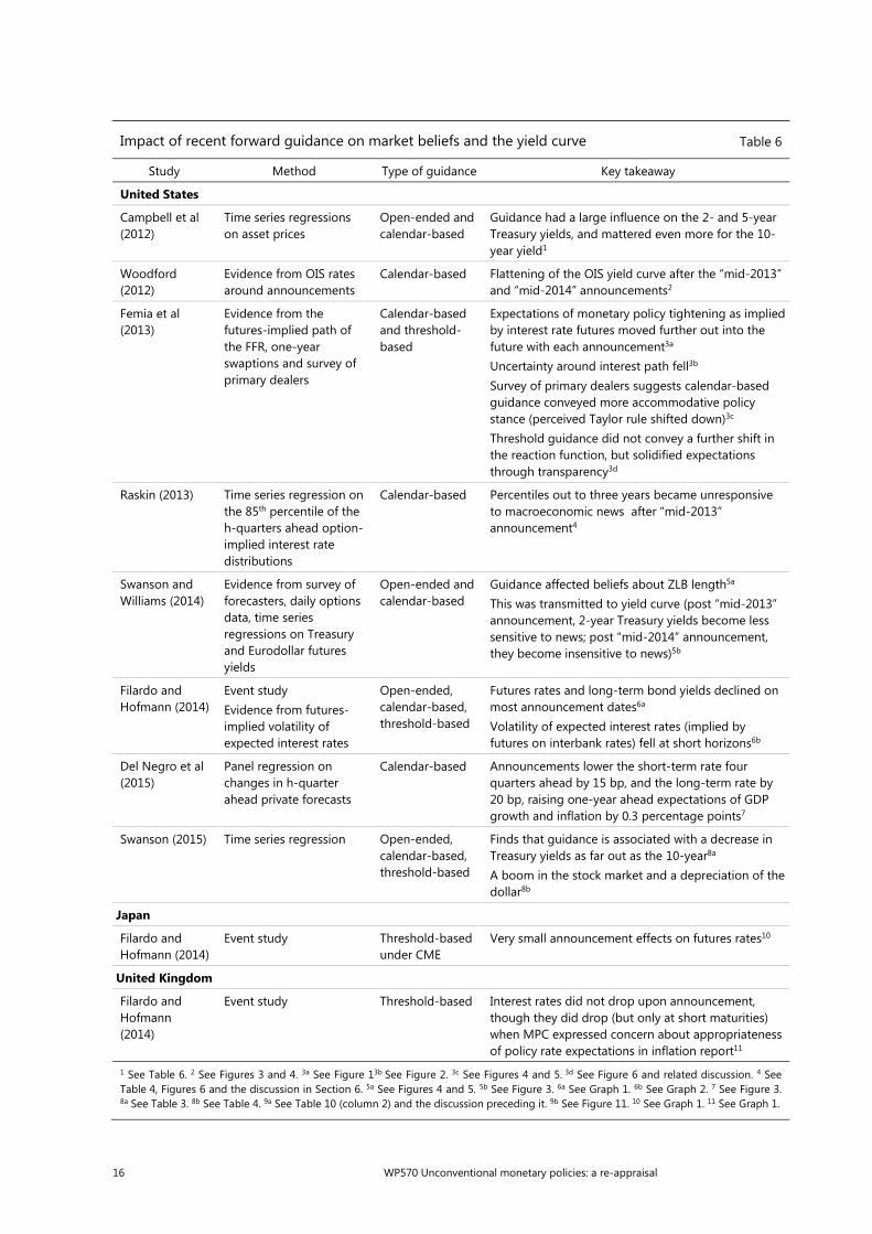
The formal evidence suggests that forward guidance can generally succeed in influencing bond yields in the right direction, but with some qualifications (Table 6). The evidence has typically been positive for the United States, a bit more mixed for Japan and, given the very limited studies available, less clear for the euro area and, even more so, for the United Kingdom. In addition, it does appear that guidance can help make markets less responsive to economic news, keeping their focus on the authorities’ charted course.
At least two factors may explain why forward guidance need not be as effective as originally hoped.
The guidance may not be fully understood. This may be the case, in particular, if it is too complex or state-contingent, as the conditions envisaged may not be expressed very clearly. After all, the central bank may wish to retain sufficient flexibility to respond to unforeseen circumstances and, in the case of committee decision-making, it might be difficult to reach agreements and compromises. 14 Qualifiers like “substantial” or “sufficient” are intentionally fuzzy. Fuzziness and ambiguity also weaken the force of announcements.
Even if understood, the guidance may not be fully believed. For one, the central bank may not be able to guarantee the consistency of future decisions beyond short
13 That said, purchases of long-term assets, for example, could be interpreted as a commitment to keep
interest rates low for a while, since the central bank would incur losses by raising rates. For this suggestion, see, for instance, Clouse et al (2003) and for a formal treatment, Bhattarai et al (2015).
14 See Feroli et al (2016) for a discussion of how forward guidance, especially if calendar-based, may hurt a central bank’s reputation and credibility if it is perceived as a commitment to a certain course of action. The authors argue that if macroeconomic events change in an unexpected manner, the central bank will either have to stick to its promise – which may be suboptimal given the new circumstances – or else have to renege on it, thereby damaging its credibility.
WP570 Unconventional monetary policies: a re-appraisal 19
horizons, eg up to one or two years, especially in committee structures with high turnover. In addition, the market may not share the central bank’s view about the outlook or the workings of the economy. For instance, in both the case of the Bank of England and the Federal Reserve, employment objectives were reached considerably faster than policymakers had expected despite subdued inflation. This may undermine the central bank’s credibility and result in unwanted changes in market conditions. The issue is compounded by markets’ natural preference for calendar-based guidance and hence their tendency to translate state-contingent statements into specific time frames – after all, timing is of the essence in trading (Tucker (2013)).
These complications, and others that will be discussed later, may explain why, over time, central banks appear to have downplayed forward guidance somewhat. There has been a certain shift from the quantitative and state-contingent type to the qualitative variety. And when quantitative elements have been retained, they have tended to refer directly to the ultimate goals, such as inflation, rather than to intermediate variables. This has gone hand-in-hand with statements about the importance of retaining flexibility in light of new incoming information – “data dependence”.
Negative policy rates
Negative policy rates are the latest addition to the arsenal of unconventional monetary policy measures. Because only two of the central banks considered here have adopted them – the ECB and the Bank of Japan – and, moreover, the Bank of Japan has done so only very recently, here we discuss also the experience of Danmarks Nationalbank, the SNB and the Swedish Riksbank.15
To non-cognoscenti, the very idea that nominal interest rates can become negative must sound extremely odd. How is it possible that anyone would pay for the privilege of parting with his or her money? In fact, to simplify, the possibility arises because the central bank can determine the quantity of bank reserves in the system and there is nothing banks can do to avoid holding them – the banking system as a whole is simply stuck with them.16 The central bank can then charge negative interest on them – in effect, a form of tax. As banks seek, unsuccessfully, to avoid the tax, the negative interest rate spreads to other rates in the economy through arbitrage relationships.
This, however, does not mean that interest rates can be set at any negative level. Far from it. Quite apart from undesirable economic and broader consequences (see below), there are technical constraints. If, in order to preserve their profitability or to avoid making losses, banks pass on the negative rates to their depositors, at some point these will shift into cash, squeezing the banks’ sources of funding. Where that point is, exactly, is unclear. It will depend on the attractiveness of cash as a settlement medium, on storage and insurance costs and on other psychological and institutional factors (eg McAndrews (2015), Rognlie (2015)). But the lower the rates sink into
15 This section draws on Bech and Malkhozov (2016), who provide a detailed analysis of the
implementation of negative policy rates and of their transmission to other rates.
16 This, of course, is just another way of saying that the central bank has full control over the amount of bank reserves, which is the key to set the policy rate (eg Borio (1997), Borio and Disyatat (2010), among many others).
20 WP570 Unconventional monetary policies: a re-appraisal
negative territory and the longer they are expected to remain there, the higher the likelihood that the shift will occur, as this makes it more advantageous to incur the fixed (sunk) costs needed to facilitate holding and storing cash.
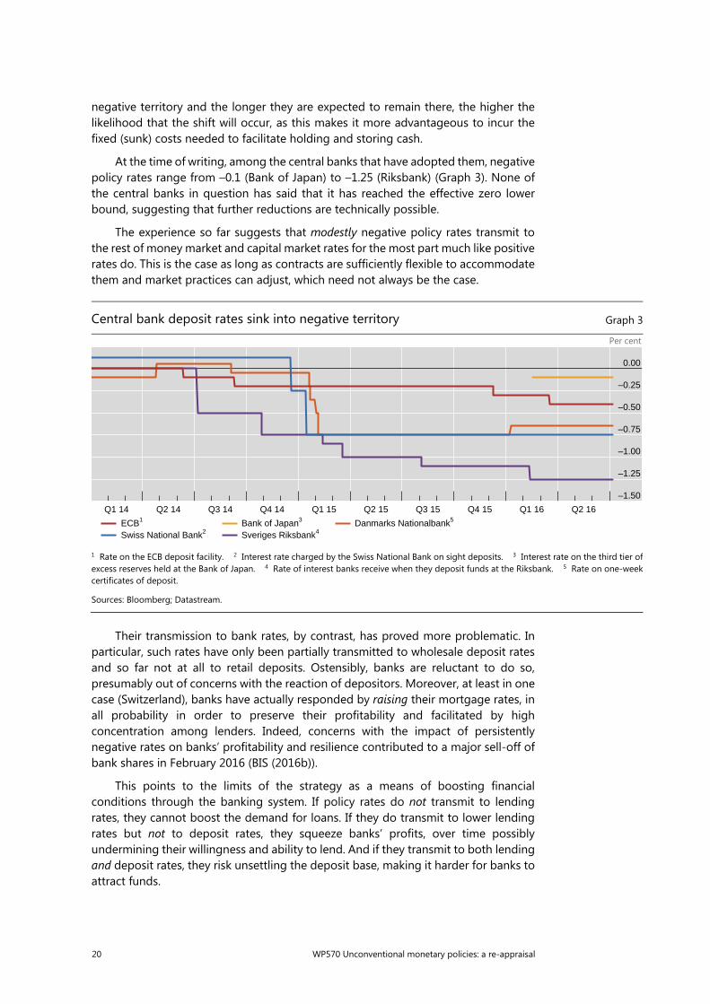
At the time of writing, among the central banks that have adopted them, negative policy rates range from –0.1 (Bank of Japan) to –1.25 (Riksbank) (Graph 3). None of the central banks in question has said that it has reached the effective zero lower bound, suggesting that further reductions are technically possible.
The experience so far suggests that modestly negative policy rates transmit to the rest of money market and capital market rates for the most part much like positive rates do. This is the case as long as contracts are sufficiently flexible to accommodate them and market practices can adjust, which need not always be the case.
Their transmission to bank rates, by contrast, has proved more problematic. In particular, such rates have only been partially transmitted to wholesale deposit rates and so far not at all to retail deposits. Ostensibly, banks are reluctant to do so, presumably out of concerns with the reaction of depositors. Moreover, at least in one case (Switzerland), banks have actually responded by raising their mortgage rates, in all probability in order to preserve their profitability and facilitated by high concentration among lenders. Indeed, concerns with the impact of persistently negative rates on banks’ profitability and resilience contributed to a major sell-off of bank shares in February 2016 (BIS (2016b)).
This points to the limits of the strategy as a means of boosting financial conditions through the banking system. If policy rates do not transmit to lending rates, they cannot boost the demand for loans. If they do transmit to lower lending rates but not to deposit rates, they squeeze banks’ profits, over time possibly undermining their willingness and ability to lend. And if they transmit to both lending and deposit rates, they risk unsettling the deposit base, making it harder for banks to attract funds.
Central bank deposit rates sink into negative territory Graph 3
Per cent
1 Rate on the ECB deposit facility. 2 Interest rate charged by the Swiss National Bank on sight deposits. 3 Interest rate on the third tier of excess reserves held at the Bank of Japan. 4 Rate of interest banks receive when they deposit funds at the Riksbank. 5 Rate on one-week certificates of deposit.
Sources: Bloomberg; Datastream.
–1.50
–1.25
–1.00
–0.75
–0.50
–0.25
0.00
Q1 14 Q2 14 Q3 14 Q4 14 Q1 15 Q2 15 Q3 15 Q4 15 Q1 16 Q2 16
ECB1
Swiss National Bank2Bank of Japan3
Sveriges Riksbank4Danmarks Nationalbank5
WP570 Unconventional monetary policies: a re-appraisal 21
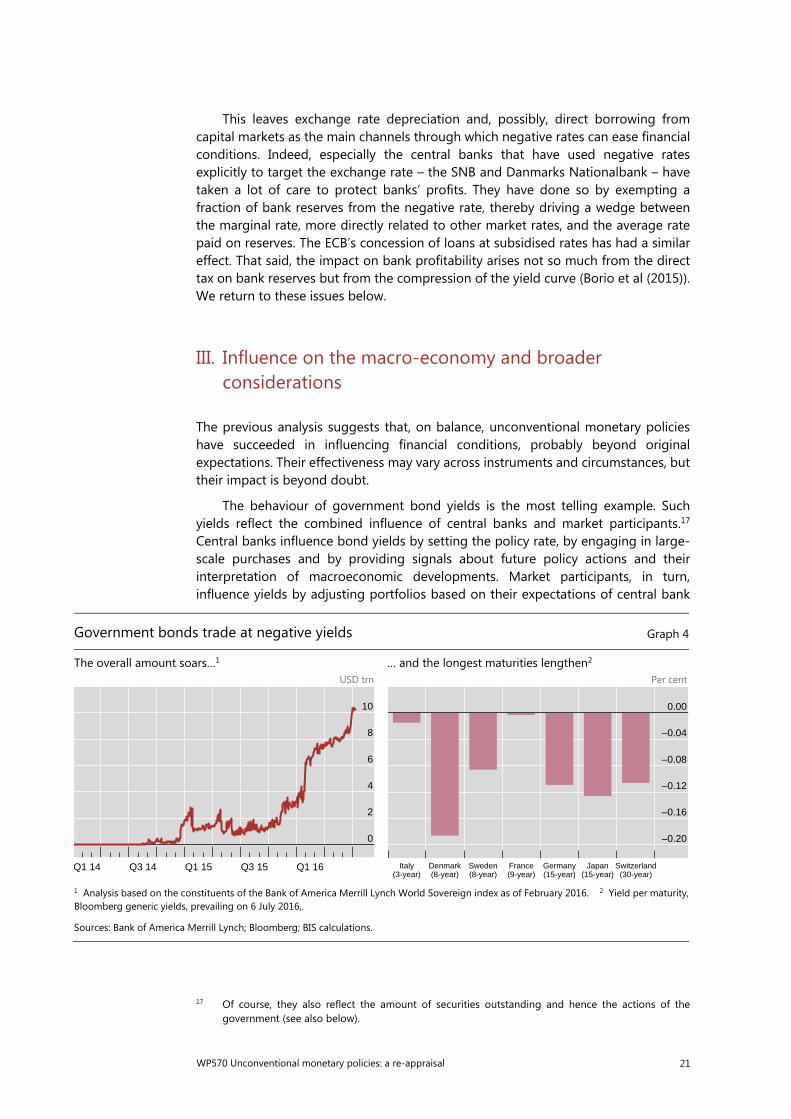
This leaves exchange rate depreciation and, possibly, direct borrowing from capital markets as the main channels through which negative rates can ease financial conditions. Indeed, especially the central banks that have used negative rates explicitly to target the exchange rate – the SNB and Danmarks Nationalbank – have taken a lot of care to protect banks’ profits. They have done so by exempting a fraction of bank reserves from the negative rate, thereby driving a wedge between the marginal rate, more directly related to other market rates, and the average rate paid on reserves. The ECB’s concession of loans at subsidised rates has had a similar effect. That said, the impact on bank profitability arises not so much from the direct tax on bank reserves but from the compression of the yield curve (Borio et al (2015)). We return to these issues below.
III. Influence on the macro-economy and broader considerations
The previous analysis suggests that, on balance, unconventional monetary policies have succeeded in influencing financial conditions, probably beyond original expectations. Their effectiveness may vary across instruments and circumstances, but their impact is beyond doubt.
The behaviour of government bond yields is the most telling example. Such yields reflect the combined influence of central banks and market participants.17 Central banks influence bond yields by setting the policy rate, by engaging in large-scale purchases and by providing signals about future policy actions and their interpretation of macroeconomic developments. Market participants, in turn, influence yields by adjusting portfolios based on their expectations of central bank
17 Of course, they also reflect the amount of securities outstanding and hence the actions of the
government (see also below).
Government bonds trade at negative yields Graph 4
The overall amount soars…1 … and the longest maturities lengthen2 USD trn Per cent
1 Analysis based on the constituents of the Bank of America Merrill Lynch World Sovereign index as of February 2016. 2 Yield per maturity, Bloomberg generic yields, prevailing on 6 July 2016,.
Sources: Bank of America Merrill Lynch; Bloomberg; BIS calculations.
0
2
4
6
8
10
Q1 14 Q3 14 Q1 15 Q3 15 Q1 16
–0.20
–0.16
–0.12
–0.08
–0.04
0.00
Italy Denmark Sweden France Germany Japan Switzerland(3-year) (8-year) (8-year) (9-year) (15-year) (15-year) (30-year)
22 WP570 Unconventional monetary policies: a re-appraisal
policy, their views about the other factors driving yields, including the macro-economy, their attitude towards risk and various balance sheet constraints. Clearly, central banks may not control such yields closely, but have a heavy thumb on the scale. Otherwise it would hardly be possible to explain how, in early July 2016, over USD 10 trillion of sovereign paper was trading at negative rates, in some cases far out the maturity spectrum, even up to 30 years, in Switzerland (Graph 4).
The more fundamental questions, though, are whether such policies have been effective in attaining central banks’ ultimate objectives, couched in terms of output and inflation, and what their limitations might be. These are much harder to answer – judgment plays a much bigger role. We next turn to them, by first examining the (limited) formal empirical evidence and then by widening the focus to explore broader considerations, including of a political economy nature.
Formal empirical evidence on output and inflation
While the literature on the impact of unconventional monetary policies on financial conditions is vast, that on their effect on output and inflation is much more limited. This largely reflects the difficulties involved.
At the cost of some oversimplification, three types of approaches are possible (Table 7).
At one end of the spectrum, one can seek to measure directly the effects of the variables of interest on output and inflation. For instance, for balance sheet policies one can examine the effect of changes in the size and structure of the central bank’s balance sheet on output and inflation, typically in a small system of equations that trace the main regularities in the data. A handful of studies have followed this route, and found evidence of effects in the desired direction (Table 7). A specific problem with such studies is that the relationship between the variables of interest is bound to be highly unstable and to exhibit breaks. As the decoupling principle indicates, there need be no stable link, and definitely no causal link, between the policy rate and the size and structure of the central bank’s balance sheet. So, any patterns observed in the period preceding the adoption of balance sheet policies are highly suspect and bound to change following their implementation. Thus, it is not clear what these studies really capture.
At the other end, one can follow a theory-based approach. In this case, one embeds a specific view of how balance sheet policies are expected to work in a general equilibrium model of the economy and then traces their effect through the system. Recently, some studies have begun to follow this approach. The corresponding models, however, are not taken to the data directly, and rely on other information to set the size of the key parameters (“calibration”), as in eg Gertler and Karadi (2013). The results, therefore, are primarily intended to shed light on the transmission mechanisms involved and are less useful as a guide to the actual size of the effects. They are best regarded as setting the basis for more refined empirical work.
An approach that lies somewhere in between is to follow a two-step procedure. One first maps the specific measures into more traditional variables or “shocks” normally included in models and econometric work; then, based on this mapping, one traces the effect on output and inflation. For example, a number of studies have mapped balance sheet policies into a synthetic (or “shadow”) policy rate. The
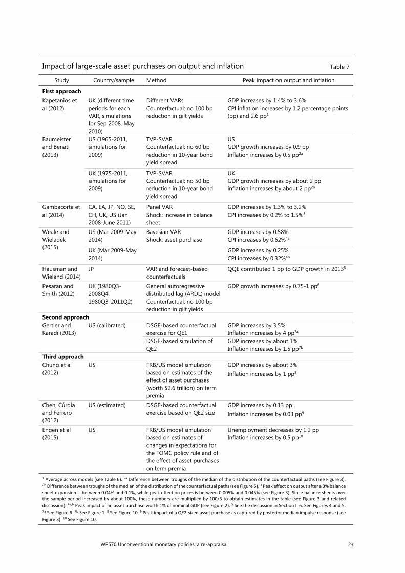
WP570 Unconventional monetary policies: a re-appraisal 23
Impact of large-scale asset purchases on output and inflation Table 7
Study Country/sample Method Peak impact on output and inflation
First approach Kapetanios et al (2012)
UK (different time periods for each VAR, simulations for Sep 2008, May 2010)
Different VARs Counterfactual: no 100 bp reduction in gilt yields
GDP increases by 1.4% to 3.6% CPI inflation increases by 1.2 percentage points (pp) and 2.6 pp1
Baumeister and Benati (2013)
US (1965-2011, simulations for 2009)
TVP-SVARCounterfactual: no 60 bp reduction in 10-year bond yield spread
USGDP growth increases by 0.9 pp Inflation increases by 0.5 pp2a
UK (1975-2011, simulations for 2009)
TVP-SVARCounterfactual: no 50 bp reduction in 10-year bond yield spread
UKGDP growth increases by about 2 pp inflation increases by about 2 pp2b
Gambacorta et al (2014)
CA, EA, JP, NO, SE, CH, UK, US (Jan 2008-June 2011)
Panel VARShock: increase in balance sheet
GDP increases by 1.3% to 3.2% CPI increases by 0.2% to 1.5%3
Weale and Wieladek (2015)
US (Mar 2009-May 2014)
Bayesian VARShock: asset purchase
GDP increases by 0.58% CPI increases by 0.62%4a
UK (Mar 2009-May 2014)
GDP increases by 0.25% CPI increases by 0.32%4b
Hausman and Wieland (2014)
JP VAR and forecast-based counterfactuals
QQE contributed 1 pp to GDP growth in 20135
Pesaran and Smith (2012)
UK (1980Q3-2008Q4, 1980Q3-2011Q2)
General autoregressive distributed lag (ARDL) model Counterfactual: no 100 bp reduction in gilt yields
GDP growth increases by 0.75-1 pp6
Second approach Gertler and Karadi (2013)
US (calibrated) DSGE-based counterfactual exercise for QE1
GDP increases by 3.5% Inflation increases by 4 pp7a
DSGE-based simulation of QE2
GDP increases by about 1% Inflation increases by 1.5 pp7b
Third approach Chung et al (2012)
US FRB/US model simulation based on estimates of the effect of asset purchases (worth $2.6 trillion) on term premia
GDP increases by about 3% Inflation increases by 1 pp8
Chen, Cúrdia and Ferrero (2012)
US (estimated) DSGE-based counterfactual exercise based on QE2 size
GDP increases by 0.13 pp Inflation increases by 0.03 pp9
Engen et al (2015)
US FRB/US model simulation based on estimates of changes in expectations for the FOMC policy rule and of the effect of asset purchases on term premia
Unemployment decreases by 1.2 pp Inflation increases by 0.5 pp10
1 Average across models (see Table 6). 2a Difference between troughs of the median of the distribution of the counterfactual paths (see Figure 3). 2b Difference between troughs of the median of the distribution of the counterfactual paths (see Figure 5). 3 Peak effect on output after a 3% balance sheet expansion is between 0.04% and 0.1%, while peak effect on prices is between 0.005% and 0.045% (see Figure 3). Since balance sheets over the sample period increased by about 100%, these numbers are multiplied by 100/3 to obtain estimates in the table (see Figure 3 and related discussion). 4a,b Peak impact of an asset purchase worth 1% of nominal GDP (see Figure 2). 5 See the discussion in Section II 6. See Figures 4 and 5. 7a See Figure 6. 7b See Figure 1. 8 See Figure 10. 9 Peak impact of a QE2-sized asset purchase as captured by posterior median impulse response (see Figure 3). 10 See Figure 10.
24 WP570 Unconventional monetary policies: a re-appraisal
reliability of the method depends critically on the quality of the mapping. This may be highly problematic. In particular, the decoupling principle undermines attempts to derive the shadow rate from the size and structure of the central bank’s balance sheet. The approach is more reliable when the mapping is simpler (eg when the model already contains a bond rate).
The bottom line is that these results generally have to be taken with more than a pinch of salt. The more data-dependent methods rely heavily on unreliable extrapolation from previous relationships. And the more theory-based ones are better regarded as illuminating the mechanisms at work. There is clearly an effect, but its size and stability are quite uncertain.
The importance of context and measure-specific characteristics
The limitations of the evidence discussed so far are one reason for the widely differing views concerning the measures’ effectiveness. There is general agreement that central bank actions, which naturally relied heavily on unconventional policies, were essential during the crisis management phase. At the time, the measures prevented the financial system from imploding and dragging down the economy. The steps were simply an extension of the traditional lender of last resort role, adapted to the specific circumstances. By contrast, views differ widely concerning the measures’ effectiveness in steering output and inflation beyond the crisis management phase. In particular, a common impression is that despite central banks having deployed the tools vigorously and beyond what was imaginable pre-crisis, output growth has remained disappointing and inflation stubbornly below objectives.
To help understand this disappointment, we need to delve deeper into the broader economic context and the specific characteristics of the measures.
Context here largely means the laborious recovery from a balance sheet recession (Borio (2014a)). The recession ushered in by the financial crisis is less amenable to traditional monetary policy measures because of the legacy of the previous financial boom. Easier monetary conditions struggle with an impaired banking system, which obstructs the transmission of policy and misallocates credit – the basic constraint is capital rather than liquidity.18 Easier conditions also have a hard time stimulating an overly indebted private sector, focused on repairing balance sheets rather than spending. And they cannot do much to correct the misallocation of resources fostered by the boom (Borio, Kharroubi, Upper and Zampolli (2016)); think, for instance, of idle cranes in a bloated construction sector. Policymakers can push hard on the accelerator, but they may fail to get the hoped-for traction.19
The measure-specific characteristics suggest that the tools may be subject to diminishing returns (eg BIS (2016a)). In some cases, this may reflect the evolution of economic conditions. For instance, some argue that balance sheet measures are likely
18 This is not to say that the measures cannot help banks in the short term, not least by generating
capital gains. Rather, the point is that over time the real solution is to recognise losses, recapitalise the institutions and restore underlying profitability – tasks that easy monetary policy cannot accomplish and may even contribute to delaying.
19 As discussed in detail elsewhere, the heavy reliance on monetary policy post-crisis has reflected the failure of other policies to take their fair share of the burden. See, for instance, Borio (2014a) and BIS (2016a).
WP570 Unconventional monetary policies: a re-appraisal 25
to be most effective when financial markets are segmented and dislocated, so that the authorities’ intervention can help alleviate the corresponding distortions.20 But more generally, there is clearly a limit to how far risk premia can be compressed, expectations guided and interest rates pushed into negative territory. As those physiological limits are approached, policy loses effectiveness and trade-offs worsen.
An obvious such example is the measures’ impact on the financial system’s profitability, resilience and hence ability to support the economy. We have already discussed the effect of persistently negative policy rates on banks (eg Borio et al (2015)). And such rates, and ultra-low yields more generally, also have a bigger debilitating effect on insurance companies and pension funds, whose liabilities have a longer maturity than their assets (eg EIOPA (2014)). The plight of pension funds is especially telling. It makes much more transparent the need for households to save more for retirement, which could weigh down on consumption (Rajan (2013)),21 and for sponsoring companies to replenish any underfunding, which could weigh down on investment.22
The pension fund example highlights the broader possibility of counterproductive effects on confidence – hardly captured by the formal macroeconomic models used to estimate the effects by extrapolating from more normal times. Take, for instance, forward guidance. Even when it is fully understood and credible, it may have unintended consequences. For, in order to convince markets that interest rates will remain unusually low for unusually long, the central bank may need to paint a rather bleak picture of the outlook. Paradoxically, the more credible the central bank is, the larger this effect is likely to be. Or take negative policy rates. The adoption of such extraordinary measures is unlikely to convey a reassuring message about the state of the economy, especially to those economic agents unfamiliar with the typical economist’s way of thinking – thinking in which real (inflation-adjusted) variables are the only thing that matters for behaviour (Box 1).
This analysis points to a couple of conclusions.
First, it suggests that, over time, as the power of the measures through domestic channels diminishes, policy may end up de facto relying more on exchange rate depreciation – not necessarily by design, but simply by default. This appears to have happened. It is no coincidence, perhaps, that exchange rates have been increasingly prominent in central bank statements (BIS (2016a)). Globally, however, this has presented problems of its own. Depreciation may result in unwelcome appreciation elsewhere, especially in countries struggling with the similar problems or worried about strong capital inflows as they seek to constrain the build-up of financial booms
20 For instance, in Vayanos and Vila (2009), clientele effects (ie limits to arbitrage) are driven by
arbitrageurs’ risk aversion. The higher the risk aversion, the less likely are arbitrageurs to substitute bonds across different maturities; so that the more segmented the yield curve, the more powerful quantitative easing is.
21 For instance, a recent survey indicates that only a small percentage of households would spend more if faced with negative rates and a similar percentage would actually spend less. No doubt, here confidence effects are at work too. See Cliffe (2016).
22 The macroeconomic models used nowadays simply assume that lower (real) interest rates always raise consumption by making consumption today more attractive relative to consumption tomorrow (the ”intertemporal substitution effect”). They rule out the possibility of depressing consumption as agents need to save more in order to get a given income in the future (the “income effect”). See Woodford (2003, Chapter 4) for a discussion of how consumption depends on the expected future path of real interest rates in textbook New Keynesian models.
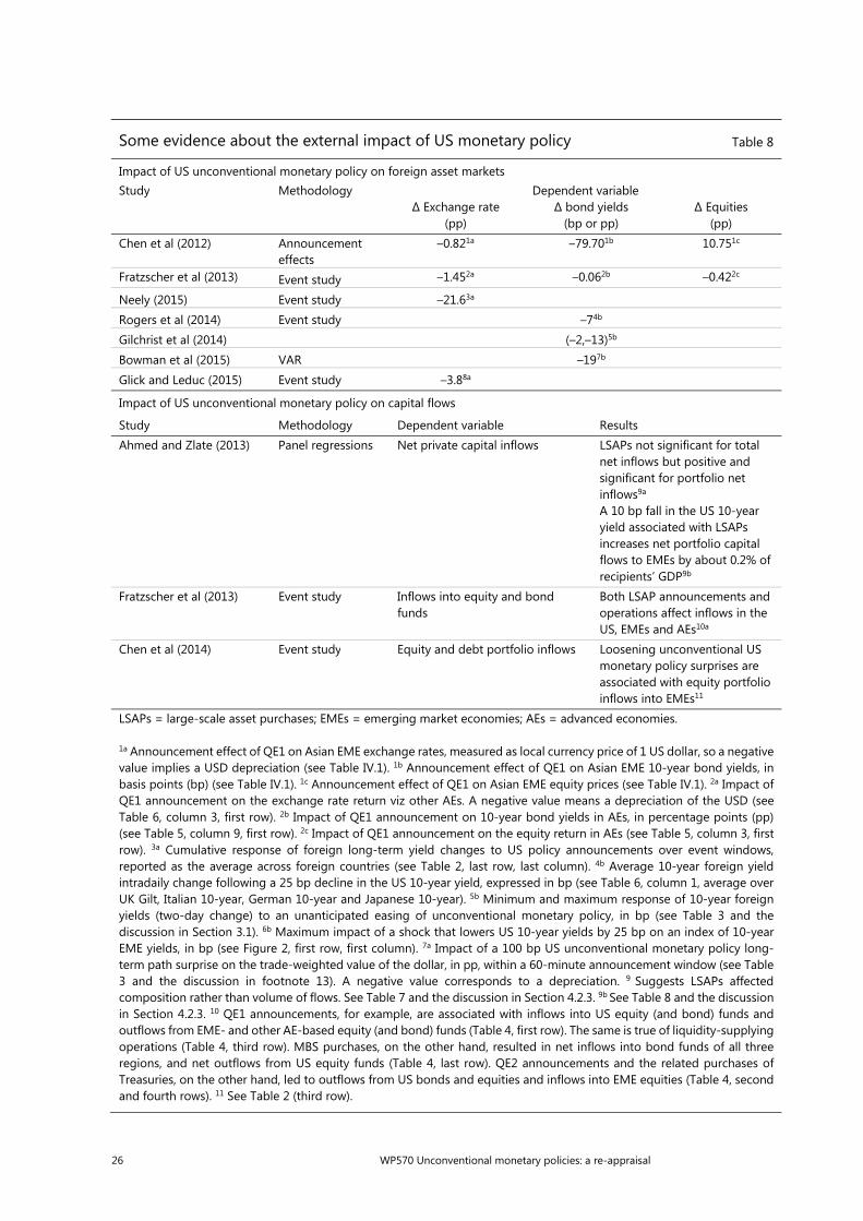
26 WP570 Unconventional monetary policies: a re-appraisal
Some evidence about the external impact of US monetary policy Table 8
Impact of US unconventional monetary policy on foreign asset markets Study Methodology Dependent variable
∆ Exchange rate (pp)
∆ bond yields (bp or pp)
∆ Equities (pp)
Chen et al (2012) Announcement effects
–0.821a –79.701b 10.751c
Fratzscher et al (2013) Event study –1.452a –0.062b –0.422c
Neely (2015) Event study –21.63a Rogers et al (2014) Event study –74b Gilchrist et al (2014) (–2,–13)5b Bowman et al (2015) VAR –197b
Glick and Leduc (2015) Event study –3.88a
Impact of US unconventional monetary policy on capital flows
Study Methodology Dependent variable Results Ahmed and Zlate (2013) Panel regressions Net private capital inflows LSAPs not significant for total
net inflows but positive and significant for portfolio net inflows9a A 10 bp fall in the US 10-year yield associated with LSAPs increases net portfolio capital flows to EMEs by about 0.2% of recipients’ GDP9b
Fratzscher et al (2013) Event study Inflows into equity and bond funds
Both LSAP announcements and operations affect inflows in the US, EMEs and AEs10a
Chen et al (2014) Event study Equity and debt portfolio inflows Loosening unconventional US monetary policy surprises are associated with equity portfolio inflows into EMEs11
LSAPs = large-scale asset purchases; EMEs = emerging market economies; AEs = advanced economies. 1a Announcement effect of QE1 on Asian EME exchange rates, measured as local currency price of 1 US dollar, so a negative value implies a USD depreciation (see Table IV.1). 1b Announcement effect of QE1 on Asian EME 10-year bond yields, in basis points (bp) (see Table IV.1). 1c Announcement effect of QE1 on Asian EME equity prices (see Table IV.1). 2a Impact of QE1 announcement on the exchange rate return viz other AEs. A negative value means a depreciation of the USD (see Table 6, column 3, first row). 2b Impact of QE1 announcement on 10-year bond yields in AEs, in percentage points (pp) (see Table 5, column 9, first row). 2c Impact of QE1 announcement on the equity return in AEs (see Table 5, column 3, first row). 3a Cumulative response of foreign long-term yield changes to US policy announcements over event windows, reported as the average across foreign countries (see Table 2, last row, last column). 4b Average 10-year foreign yield intradaily change following a 25 bp decline in the US 10-year yield, expressed in bp (see Table 6, column 1, average over UK Gilt, Italian 10-year, German 10-year and Japanese 10-year). 5b Minimum and maximum response of 10-year foreign yields (two-day change) to an unanticipated easing of unconventional monetary policy, in bp (see Table 3 and the discussion in Section 3.1). 6b Maximum impact of a shock that lowers US 10-year yields by 25 bp on an index of 10-year EME yields, in bp (see Figure 2, first row, first column). 7a Impact of a 100 bp US unconventional monetary policy long-term path surprise on the trade-weighted value of the dollar, in pp, within a 60-minute announcement window (see Table 3 and the discussion in footnote 13). A negative value corresponds to a depreciation. 9 Suggests LSAPs affected composition rather than volume of flows. See Table 7 and the discussion in Section 4.2.3. 9b See Table 8 and the discussion in Section 4.2.3. 10 QE1 announcements, for example, are associated with inflows into US equity (and bond) funds and outflows from EME- and other AE-based equity (and bond) funds (Table 4, first row). The same is true of liquidity-supplying operations (Table 4, third row). MBS purchases, on the other hand, resulted in net inflows into bond funds of all three regions, and net outflows from US equity funds (Table 4, last row). QE2 announcements and the related purchases of Treasuries, on the other hand, led to outflows from US bonds and equities and inflows into EME equities (Table 4, second and fourth rows). 11 See Table 2 (third row).
WP570 Unconventional monetary policies: a re-appraisal 27
Box 1
Delving into negative interest rates and “money illusion”
It is common in economics to assume that agents’ behaviour is, or at least should be, only a function of real (ie inflation-adjusted) variables. This is modelled, in particular, by assuming that they derive utility exclusively from real variables, such as real incomes, real money balances and the like. It is also common to treat departures from this assumption as “irrational”. For instance, an agent should be indifferent between receiving the same real income regardless of whether in one case prices have risen and in the other fallen. If the agent prefers the outcome with a higher nominal income but the same real income, then he/she is said to suffer from “money illusion” (Fisher (1928)).
Do agents disregard real quantities? Is this necessarily irrational? And what are the implications for negative interest rates? In what follows we will argue that nominal quantities do appear to matter over and above real quantities, that this need not be “irrational” but may reflect at least in part the fundamental role money plays in our economies, and that this has significant implications for the impact that negative nominal rates may have on behaviour.
There is, in fact, a voluminous literature indicating that agents behave as if they had money illusion. The evidence takes a variety of forms. One is surveys designed to tease out money illusion (eg, Shafir et al (1997), Shiller (1997)). Another is controlled experiments in the form of “games” played out within groups (eg Fehr and Tyran (2001), Noussair et al (2008) and references therein) or of a neurological character, monitoring the brain’s reactions to specific stimuli (Weber et al (2009)). Yet another is econometric studies, for instance those that examine the behaviour of asset prices, such as equity (Modigliani and Cohn (1979)), house prices (Brunnermeier and Julliard (2007)) or bonds (Shiller (2015)). In all of these cases, nominal variables, such as nominal interest rates, appear to play a role over and above real ones.
The factors that lie behind this type of behaviour are not fully understood. As often argued, psychological biases or cognitive limitations may well be at work. For instance, the price level is in fact an index computed based on the prices of a basket of goods and services, which are weighted differently depending on the intended use. Coming to grips with that concept is more complicated than dealing with dollars or pounds. But more fundamental factors may also be relevant.
One has to do with the choice of price level. A question to ask is “whose price level?”. In a world in which economic agents differ widely, the general price level need not correspond to anyone’s needs in particular. It is well known that consumer spending patterns differ greatly, depending on age, income and the like, that individual producers care about different prices, and so on. The mental experiments that lie at the heart of money illusion and are embedded in benchmark models ask “what would happen if all prices changed by a certain amount?”. Zero inflation in this sense is not the same as a much more realistic situation in which prices change by varying amounts, including in opposite directions, and they just happen to cancel out in aggregate for a particular index. In this second case, some economic agents gain, others lose. In such circumstances, even if agents do not experience money illusion, they will behave as if they do. Moreover, whenever agents do not have accurate knowledge of the behaviour of all the relevant prices, it is natural for them to rely more heavily on nominal rather than real variables.
Such considerations are likely to be especially relevant in the proximity of price stability, ie when the aggregate price level, as conventionally measured, rises or falls gradually. In fact, in this case it is almost a certainty that some prices will rise and others will fall so that, strictly speaking, there is no general increase (inflation) or decrease (deflation) as envisaged in the standard counterfactual questions asked in the models and in mental experiments.
A second factor has to do with the critical role money plays as a “unit of account”, ie as the unit in which all prices are measured, contracts are struck, and assets and liabilities denominated. Money acts as a standard unit of measurement for all the (relative) prices in the economy, greatly reducing information costs (Brunner and Meltzer (1971)). By quoting all prices relative to the same unit – the “numeraire” – the number of price quotes is dramatically cut, with clear efficiency gains. This greatly simplifies what needs to be known and communicated, much like a standard unit of measurement helps in other scientific fields and walks of life. Moreover, once the same unit is also naturally used to denominate deferred cash flow receipts (assets) in contracts, it makes sense to denominate liabilities in the same unit in order to reduce “exchange rate” risk (Doepker and Schneider (2013)). Much like, say, it makes sense for oil producers whose revenues are denominated in US dollars to incur liabilities in the same currency: by so doing, they hedge their risk. In turn, it is natural for the unit of account and medium of exchange (or settlement) to coincide.
Once contracts as well as assets and liabilities are denominated in nominal terms, then they take on a life of their own in influencing behaviour. The corresponding nominal “inertia” and “rigidities” are, in fact, a reflection of the deep
28 WP570 Unconventional monetary policies: a re-appraisal
(eg Borio (2014b), Rey (2013), Bruno and Shin (2012)). Indeed, there is evidence that large-scale asset purchases have affected not just exchange rates, but also capital flows and asset prices in other countries (Table 8). In turn, unwelcome exchange rate appreciation can induce other countries to ease policy in order to fend it off. Hence the frequent references to “currency wars” and “competitive depreciations” (eg Rajan (2014)). This helps explain why monetary policy has looked unusually easy globally, regardless of benchmarks (eg Hofmann and Bogdanova (2012), Taylor (2013), Borio (2016)).
Second, it also suggests that, over time, the balance between the benefits and costs of the measures deteriorates. The effectiveness tends to diminish, especially as the policy room for manoeuvre narrows. And any side-effects tend to grow – on the profitability and resilience of the financial system, on risk-taking in financial markets and on the global balance of policies (eg Borio (2014a), Borio and Disyatat (2014)). Ultimately, this may undermine the credibility of central banks.23
23 There is, indeed, some evidence consistent with this view (see BIS (2016a), Chapter IV). The impact of
the measures on output and inflation appears to have declined in some countries (eg Hofmann and Weber (2016)) while that on the exchange rate has not. Similarly, there is evidence that the impact of interest rates on lending weakens as they fall to very low levels and squeeze net interest margins (Borio and Gambacorta (2016)).
and pervasive role money plays in our fundamentally monetary economies. The strength of the underlying forces helps explain what would otherwise be a puzzling phenomenon, ie the limited reach and fragility of indexation mechanisms (Shiller (1997)).
The analysis also sheds light on why nominal interest rates may be relevant for behaviour quite apart from real interest rates. And it indicates that the instinctive aversion to negative interest rates has deep roots in how our economies work, rather than being just a sign of irrational behaviour. Likewise, zero may not just be a point along a seamless continuum, but have a significance of its own: it marks the difference between receiving something in exchange for the sacrifice of parting with one’s money and paying for the corresponding “privilege”, between encouraging the use of the unit of account and discouraging it.
One possible implication is that negative rates may adversely affect behaviour in ways that would not be understood if one reasoned purely in real terms. Regardless of whether inflation is positive or negative, negative nominal rates are likely to be perceived as a “tax” – a more visible one than that associated with inflation, as conventionally measured. This also raises huge communication challenges for policymakers who resort to them in order to boost inflation. One rationale for adopting low inflation objectives is precisely to reduce the hidden tax inflation levies on the population, as it erodes the purchasing power of income and wealth. With negative interest rates put in place in order to boost inflation, it is as if economic agents were taxed twice. The justification relies on models in which negative real rates would generate better economic outcomes and whose rationale, therefore, needs to be convincingly explained.
A second implication is that the prospect of setting interest rates at any negative level as a means of boosting output would risk backfiring and undermining the functioning of the economy. This option has been proposed, in particular, to address the debt overhang problem (Rogoff (2014)). More generally, it is the logical implication of models in which it is only real variables that influence behaviour. Our analysis points to potentially far-reaching consequences of the prospect of charging a tax of, in principle, an unconstrained size on the holdings of the settlement medium which, in turn, coincides with the unit of account. This is the medium on which the whole economic edifice is built.
Lucas (1972) famously developed a model along these lines, in which agents could only observe a sub-set of prices (from their “information islands”) and hence sought to distinguish general from relative price changes based on the imperfect information available to them. The depressing effect of persistently negative interest rates on bank profitability in the text is just one example of the far-reaching effect of these forces. This argument is distinct from the other implications resulting from the mechanisms needed to implement the measure. One that has attracted much attention is the potential loss of privacy linked to the elimination of cash (eg Cochrane (2014)).
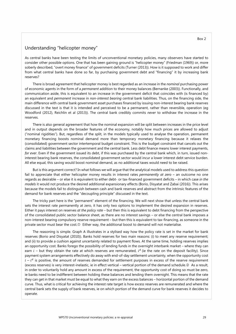
WP570 Unconventional monetary policies: a re-appraisal 29
Box 2
Understanding “helicopter money”
As central banks have been testing the limits of unconventional monetary policies, many observers have started to consider other possible options. One that has been gaining ground is “helicopter money” (Friedman (1969)) or, more soberly described, “overt money finance” of government deficits (Turner (2013)). How is it supposed to work and differ from what central banks have done so far, by purchasing government debt and “financing” it by increasing bank reserves?
There is broad agreement that helicopter money is best regarded as an increase in the nominal purchasing power of economic agents in the form of a permanent addition to their money balances (Bernanke (2003)). Functionally, and communication aside, this is equivalent to an increase in the government deficit that coincides with (is financed by) an equivalent and permanent increase in non-interest bearing central bank liabilities. Thus, on the financing side, the main difference with central bank government asset purchases financed by issuing non-interest bearing bank reserves discussed in the text is that it is intended and perceived to be a permanent, rather than reversible, operation (eg Woodford (2012), Reichlin et al (2013)). The central bank credibly commits never to withdraw the increase in the reserves.
There is also general agreement that how the nominal expansion will be split between increases in the price level and in output depends on the broader features of the economy, notably how much prices are allowed to adjust (“nominal rigidities”). But, regardless of the split, in the models typically used to analyse the operation, permanent monetary financing boosts nominal demand more than temporary monetary financing because it relaxes the (consolidated) government sector intertemporal budget constraint. This is the budget constraint that cancels out the claims and liabilities between the government and the central bank. Less debt finance means lower interest payments, for ever. Even if the government issued its debt, if this was purchased by the central bank which, in turn, issued non-interest bearing bank reserves, the consolidated government sector would incur a lower interest debt service burden. All else equal, this saving would boost nominal demand, as no additional taxes would need to be raised.
But is this argument correct? In what follows we will argue that the analytical models used to address this question fail to appreciate that either helicopter money results in interest rates permanently at zero – an outcome no one regards as desirable – or else it is equivalent to either debt- or tax-financed government deficits – in which case in the models it would not produce the desired additional expansionary effects (Borio, Disyatat and Zabai (2016)). This arises because the models fail to distinguish between cash and bank reserves and abstract from the intrinsic features of the demand for bank reserves and the “decoupling principle” discussed in the text.
The tricky part here is the “permanent” element of the financing. We will next show that unless the central bank sets the interest rate permanently at zero, it has only two options to implement the desired expansion in reserves. Either it pays interest on reserves at the policy rate – but then this is equivalent to debt financing from the perspective of the consolidated public sector balance sheet, as there are no interest savings – or else the central bank imposes a non-interest bearing compulsory reserve requirement – but then this is equivalent to tax-financing, as someone in the private sector must bear the cost. Either way, the additional boost to demand will not materialise.
The reasoning is simple. Graph A illustrates in a stylised way how the policy rate is set in the market for bank reserves (Borio and Disyatat (2010)). Banks hold reserves for two main reasons: (i) to meet any reserve requirement; and (ii) to provide a cushion against uncertainty related to payment flows. At the same time, holding reserves implies an opportunity cost. Banks forego the possibility of lending funds in the overnight interbank market – where they can earn – but they obtain the rate at which reserves are remunerated, (ie the rate on the deposit facility). Since payment system arrangements effectively do away with end-of-day settlement uncertainty, when the opportunity cost − is positive, the amount of reserves demanded for settlement purposes in excess of the reserve requirement (excess reserves) is very interest-inelastic, ie in effect vertical – vertical portion of the demand schedule. As a result, in order to voluntarily hold any amount in excess of the requirement, the opportunity cost of doing so must be zero, ie banks need to be indifferent between holding these balances and lending them overnight. This means that the rate they can get in that market must be equal to what they earn on the excess balances – horizontal portion of the demand curve. Thus, what is critical for achieving the interest rate target is how excess reserves are remunerated and where the central bank sets the supply of bank reserves, ie on which portion of the demand curve for bank reserves it decides to operate.
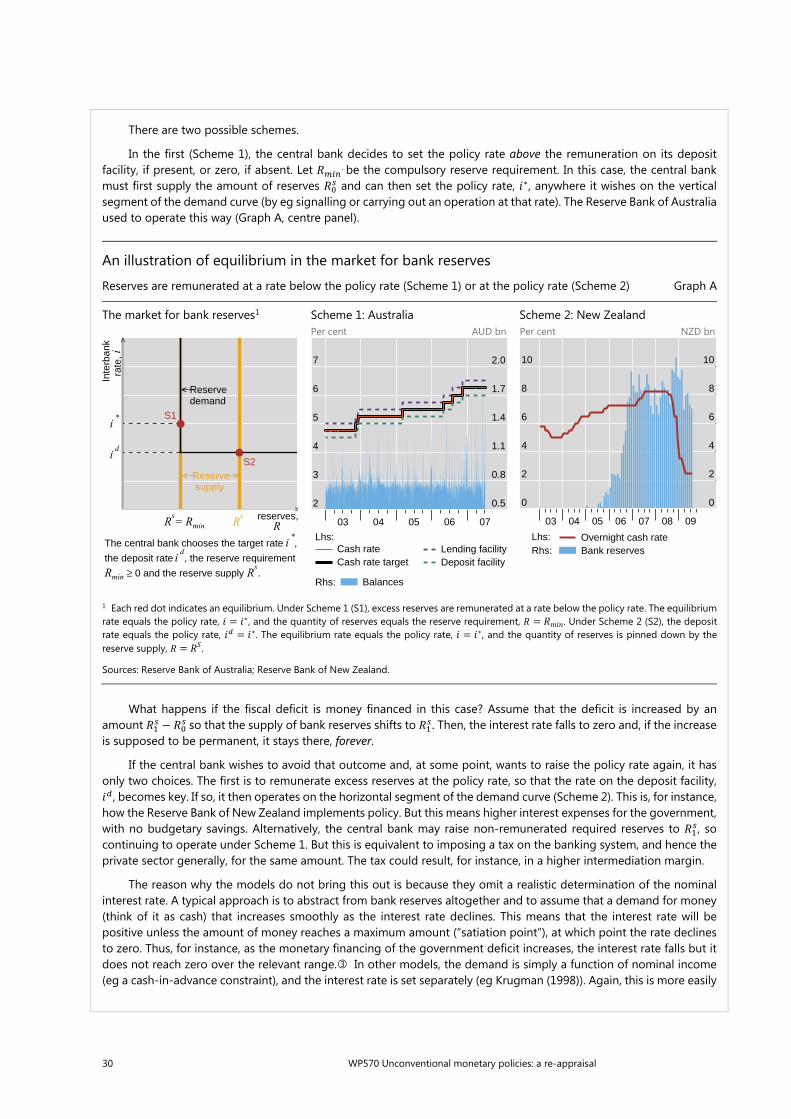
30 WP570 Unconventional monetary policies: a re-appraisal
There are two possible schemes.
In the first (Scheme 1), the central bank decides to set the policy rate above the remuneration on its deposit facility, if present, or zero, if absent. Let . be the compulsory reserve requirement. In this case, the central bank must first supply the amount of reserves and can then set the policy rate, ∗, anywhere it wishes on the vertical segment of the demand curve (by eg signalling or carrying out an operation at that rate). The Reserve Bank of Australia used to operate this way (Graph A, centre panel).
What happens if the fiscal deficit is money financed in this case? Assume that the deficit is increased by an amount − so that the supply of bank reserves shifts to . Then, the interest rate falls to zero and, if the increase is supposed to be permanent, it stays there, forever.
If the central bank wishes to avoid that outcome and, at some point, wants to raise the policy rate again, it has only two choices. The first is to remunerate excess reserves at the policy rate, so that the rate on the deposit facility,
, becomes key. If so, it then operates on the horizontal segment of the demand curve (Scheme 2). This is, for instance, how the Reserve Bank of New Zealand implements policy. But this means higher interest expenses for the government, with no budgetary savings. Alternatively, the central bank may raise non-remunerated required reserves to , so continuing to operate under Scheme 1. But this is equivalent to imposing a tax on the banking system, and hence the private sector generally, for the same amount. The tax could result, for instance, in a higher intermediation margin.
The reason why the models do not bring this out is because they omit a realistic determination of the nominal interest rate. A typical approach is to abstract from bank reserves altogether and to assume that a demand for money (think of it as cash) that increases smoothly as the interest rate declines. This means that the interest rate will be positive unless the amount of money reaches a maximum amount (“satiation point”), at which point the rate declines to zero. Thus, for instance, as the monetary financing of the government deficit increases, the interest rate falls but it does not reach zero over the relevant range. In other models, the demand is simply a function of nominal income (eg a cash-in-advance constraint), and the interest rate is set separately (eg Krugman (1998)). Again, this is more easily
An illustration of equilibrium in the market for bank reserves
Reserves are remunerated at a rate below the policy rate (Scheme 1) or at the policy rate (Scheme 2) Graph A
The market for bank reserves1 Scheme 1: Australia Scheme 2: New Zealand Per cent AUD bn Per cent NZD bn
1 Each red dot indicates an equilibrium. Under Scheme 1 (S1), excess reserves are remunerated at a rate below the policy rate. The equilibrium rate equals the policy rate, = ∗, and the quantity of reserves equals the reserve requirement, = . Under Scheme 2 (S2), the deposit rate equals the policy rate, = ∗. The equilibrium rate equals the policy rate, = ∗, and the quantity of reserves is pinned down by the reserve supply, = .
Sources: Reserve Bank of Australia; Reserve Bank of New Zealand.
>
>
Inte
rban
k r
ate,
reserves,
i
Rs= Rmin R
i *
i d
Reservedemand
Reserve supply
__<
<__
The central bank chooses the target rate ,
the deposit rate , the reserve requirement
≥ 0 and the reserve supply .
i * i d
>__
S1
S2
Rs
Rmin Rs
2
3
4
5
6
7
0.5
0.8
1.1
1.4
1.7
2.0
03 04 05 06 07
Rhs:
Cash rateCash rate target
Lhs:Lending facilityDeposit facility
Balances
0
2
4
6
8
10
0
2
4
6
8
10
03 04 05 06 07 08 09
Lhs:Rhs:
Overnight cash rate Bank reserves
WP570 Unconventional monetary policies: a re-appraisal 31
The combination of context and measure-specific characteristics raises serious exit issues. On the one hand, it is compelling for central banks to press further on the accelerator in order to achieve their objectives. Naturally, if inflation remains stubbornly below target, they may hardly see any alternative. Failing to press further could be viewed as signalling the measures’ ineffectiveness and that central banks have given up on their mandates. Markets could then lose confidence in central banks’ ability to deliver and governments could accuse them of undermining their own policies. The increasingly insistent discussion of helicopter money, regardless of its inherent merits, is just the latest example of the incentives at work (Box 2). On the other hand, unless the measures do prove sufficient or other factors come to the
rationalised if we think of money as cash (or non-interest bearing bank deposits) rather than bank excess reserves, which do not depend on either the price level or income. In fact, in real life central banks meet entirely passively the public’s demand for cash, which therefore does not influence the setting of the interest rate. If they did not, either the amount in excess of desired balances would end up with the banks, and effectively be switched into excess reserves, or if would fall short of the demand, frustrating the public, which would presumably turn to alternative means of payment.
This analysis suggests a number of further observations.
First, the prevailing models used to justify helicopter money imply that the price of a more expansionary monetary policy is actually giving up on monetary policy forever. Once the models are complemented with a realistic interest rate-setting mechanism, a permanent money-financed fiscal programme with the desired budgetary savings can only be implemented by giving up on monetary policy forever.
Second, for much the same reasons, short of permanent financing, these models would suggest a rather limited additional expansionary impact of monetary financing.
Third, all this excludes the “choreography” of helicopter money and transmission mechanisms not included in the models. In particular, what would the impact of more overt, if still temporary, financing be? This is harder to tell. The impact on confidence is quite unpredictable. Some argue that it would be positive (eg Turner (2013)). But it might equally be negative, except perhaps in the short run. The measures could convey the sense that the economic situation is quite gloomy and requires exceptional steps. Moreover, any impact would be temporary unless the operation was repeated over and over again in size.
And therein lies the danger: this could raise questions about the broader institutional implications, including the de facto subordination of monetary to fiscal policy, with unpredictable consequences. Indeed, as widely recognised, the policy obviously undermines central bank independence. This is why proponents typically explore ways in which co-ordination could be constrained by rules and by the central bank’s decisional autonomy. In fact, central banks are generally not allowed to credit citizens’ accounts directly (eg Grenville (2013)), in the process reducing their own equity capital and putting their financial strength at risk. The reason is that the transfer, as opposed to its financing, is a quintessential fiscal task. Sooner or later, the perception of fiscal dominance could indeed erode the value of money, but at the cost of losing the public’s confidence in monetary institutions, so painfully gained over the years. If so, it would be Pyrrhic victory.
Turner (2013) explicitly sees permanent overt money finance as a way of avoiding the unwelcome consequences of low interest rates, such as excessive risk taking, encouraging more debt, etc. He makes only a passing reference in a footnote to higher reserve requirements as needed to avoid preventing an offsetting liability in the consolidated public sector balance sheet; but he does not assimilate it to a tax. In his latest book, he stresses that higher requirements are desirable in order to slow down credit expansion (Turner (2016)). This, however, is another issue and does not affect the previous discussion. For simplicity, here we avoid the complications that arise when reserve requirements have averaging provisions, which do not really affect our argument. For the details, see Borio (1997). Buiter (2014) argues that even when the rate is zero to start with, permanent increases in money financing will increase nominal aggregate demand. This is because he assumes that money – not just the additional income transfer – is valuable by itself and this will induce agents to spend more (money is included in the agent’s utility function with these properties). This, however, at most applies to cash and not to excess reserves. Moreover, the central bank simply meets the demand for cash passively. If it tried to issue more, in all probability this would simply lead the public to shift into bank deposits and banks, in turn, to ask for the central bank to replace the excess cash with more convenient electronic entries on their books.
32 WP570 Unconventional monetary policies: a re-appraisal
rescue, sooner or later their limitations would become fully apparent. The consequences would be similar. The market turbulence in February 2016, seemingly exacerbated in part by a loss of confidence in central banks’ powers, highlights the dilemmas involved (BIS (2016b)). Markets’ dependence on central bank support is hard to shake off (eg El-Erian (2016)). And even short of such loss of confidence and credibility, the narrowing room for policy manoeuvre would make it harder to address the next recession, whenever it arises, unless central banks manage to “reload the gun” ahead of time.
The political economy
Unconventional monetary policy measures also raise delicate political economy issues.24 Here, we focus on two – the policies’ perceived impact on inequality and the complications linked to balance sheet measures.
It has long been recognised that monetary policy has an impact on income and, in particular, wealth distribution. The policy’s incidence differs across segments of the population, depending on their sources of income, the amount and structure of their wealth, and their exposure to unemployment. To cite probably the best-known case, the differential impact between debtors and creditors has been analysed extensively by those exploring the political economy of monetary policy.
At the same time, as long as economic performance is satisfactory and monetary policy measures evolve within a narrow range, these issues can easily fade into the background. This is very much what happened pre-crisis, during the period of the so-called Great Moderation, as growth was generally strong and inflation low and stable.
Things have changed post-crisis. On the one hand, the financial crisis has put the spotlight on the growing inequality that had been developing for decades (eg Piketty (2014)). On the other hand, the extreme monetary policy settings have focused attention on central banks’ role, not least given their greater and explicit reliance on boosting asset prices and given the impact of persistent exceptionally low interest rates on savers. Not surprisingly, central banks have been drawn into the debate (eg Yellen (2015), Draghi (2015), Mersch (2014) and Haldane (2014)). Once again, the genie is out of the bottle.
Formal evidence on the impact of monetary policy on inequality is limited. To illustrate the issues involved, we draw on a recent study by Domanski et al (2016), which considers the link between monetary policy and wealth distribution. Through a set of simulations based on household surveys, the study concludes that wealth inequality – as measured by the difference between the wealth of the 80th and 20th percentiles in the distribution – has increased post-crisis. The impact of monetary policy is harder to pin down. But given typical portfolio configurations, it tends to raise inequality by boosting equity prices but may lower it by boosting house prices. France and, especially, Germany are exceptions in this respect, since the 20th percentile holds a smaller proportion of its wealth in both equities and real estate than the 80th percentile. In these cases, inequality increases on both counts.
24 In order to keep the paper manageable, we do not discuss those that arise in the context of credit
policies during the management of crises, involving the role of central banks in emergency liquidity provision. Rather, we focus on the deployment of tools in the performance of traditional monetary policy functions.
WP570 Unconventional monetary policies: a re-appraisal 33
This illustration highlights the communication challenges central banks face. The direct impact of policy on asset prices, especially equities, is quite visible. And if one focuses on the richest (eg, the top 1 per cent) and poorest segments of the population, it is hard to argue that policy does not raise wealth inequality. The defence has to rely on the argument that policy is sufficiently effective in boosting output and employment – a key source of income and, over time, wealth (eg Bernanke (2015), Mersch (2014)). But, regardless of its merits, it is politically difficult to counter an argument based on immediate observation with one based on a counterfactual.
The challenges balance sheet policies raise are at least as tough. They ultimately derive from a simple fact: central banks have a monopoly over interest rate policy (the policy interest rate) but not over balance sheet policy (Borio and Disyatat (2010)). Almost any balance sheet policy can, or could be, replicated by the government; conversely, any balance sheet policy has an impact on the consolidated government sector balance sheet. Balance sheet policy needs to be viewed as part of this larger balance sheet. For example, the central bank may purchase long-term bonds, but its efforts could be frustrated if government debt managers lengthened maturity in order to lock in unusually low yields (eg McCauley and Ueda (2009), Borio and Disyatat (2010) and Turner (2011)). Likewise, the government could directly intermediate funds, by borrowing in the market in order to carry out credit policies without involving the central bank.
This helps explain why balance sheet policies have a quasi-fiscal character and blur the line between the government and the central bank. If the central bank engages actively in credit policies, it may be criticised for favouring one set of borrowers over another – a concern especially acute in the United States. And it if purchases government paper on a large scale it may be criticised for financing the government – a common concern in some European countries. In the euro area, these problems are exacerbated by the co-existence of sovereigns with differing credit quality, so that purchases inevitably have distributional implications across countries.
All this puts a premium on co-ordination and raises deeper questions about central bank independence. For one, it is not entirely clear what instrument independence means in the case of balance sheet policies, given the close interrelationships between central bank and government measures and the lack of exclusive control over the instruments. More generally, extensive reliance on balance sheet policy may also threaten the central bank’s operational independence in interest rate policy.
A key channel relates to the financial risks the central bank faces. As discussed, balance sheet policy typically involves large increases in the central bank’s balance sheet. Purchases of long-term debt raise duration, and hence market, risk; credit policies, in addition, generate credit risk.25 To be sure, various mechanisms have been used to reduce credit risks (eg collateral, government guarantees against credit losses or indemnification). And the relevance of these reputational and budgetary risks is country-specific, varying with institutional and cultural factors. Even so, this does not make them less relevant.
Should one care about operational independence per se? No doubt, operational independence is only a means to an end. But experience suggests that it has a habit
25 These risks are even larger in the case of exchange rate policies, given the typical range of fluctuations
in exchange rates.
34 WP570 Unconventional monetary policies: a re-appraisal
of coming under threat precisely when it is most valuable. And loss of independence may also go hand-in-hand with a loss of legitimacy and credibility of the institution.
Conclusion
Originally, the monetary policy measures central banks adopted in the wake of the financial crisis were regarded as unconventional; almost a decade on, they have become commonplace.
We have argued that this development is a risky one. Unconventional monetary policy measures, in our view, are likely to be subject to diminishing returns. The balance between benefits and costs tends to worsen the longer they stay in place. Exit difficulties and political economy problems loom large. Short-term gain may well give way to longer-term pain. As the central bank’s policy room for manoeuvre narrows, so does its ability to deal with the next recession, which will inevitably come. The overall pressure to rely on increasingly experimental, at best highly unpredictable, at worst dangerous, measures may at some point become too strong. Ultimately, central banks’ credibility and legitimacy could come into question.
In many respects, of course, extensive reliance on unconventional monetary policies is not so much the cause but the effect of deeper fault lines. One, discussed here, is the nature of the recession and subsequent recovery ushered in by the financial crisis. Another is the unbalanced post-crisis policy mix, which left monetary policy to carry the bulk of the burden (BIS (2016a)). Yet another one has to do with the forces that have kept inflation stubbornly low and below targets – forces that are not fully understood and have drastically narrowed central banks’ options (eg BIS (2014)). But a final one is arguably the less than fully adequate character of current monetary policy frameworks – frameworks focused on short-term inflation control and that struggle to take financial stability systematically into account, despite its potentially huge macroeconomic costs (eg Borio (2016)). But this, important as it is, is another story.
WP570 Unconventional monetary policies: a re-appraisal 35
References
Abbassi, P and T Linzert (2011): "The effectiveness of monetary policy in steering money market rates during the recent financial crisis", European Central Bank Working Paper Series, no 1328.
Ahmed, S and A Zlate, Andrei (2014): "Capital flows to emerging market economies: A brave new world?", Journal of International Money and Finance, vol 48(PB), pp 221-248.
Aizenman, J and G K Pasricha (2010): "Selective swap arrangements and the global financial crisis: Analysis and interpretation", International Review of Economics and Finance, vol 19(3), pp 353-365, June.
Altavilla, C, G Carboni and R Motto (2015): "Asset purchase programmes and financial markets: lessons from the euro area", European Central Bank Working Papers, no 1864.
Angelini, P, A Nobili and C Picillo (2011): "The interbank market after august 2007: What has changed, and why?", Journal of Money, Credit and Banking, vol 43(5), pp 923-958, August.
Araújo, A, S Schommer and M Woodford (2015): "Conventional and unconventional monetary policy with endogenous collateral constraints," American Economic Journal: Macroeconomics, vol 7(1), pp 1-43, January.
Ashcraft, A, N Gârleanu, L H Pedersen (2011): "Two monetary tools: Interest rates and haircuts", NBER Macroeconomics Annual 2010, vol 25, pp 143-180.
Baba, N and F Packer (2009): "From turmoil to crisis: Dislocations in the FX swap market before and after the failure of Lehman Brothers," Journal of International Money and Finance, vol 28(8), pp 1350-1374, December.
Bank for International Settlements (2016a): 86th BIS Annual Report, Basel.
______ (2016b): Overview, BIS Quarterly Review, March.
Bauer, M D and Rudebusch, G D (2014): "The signaling channel for Federal Reserve bond purchases", International Journal of Central Banking, vol 10(3), pp 233-289, September.
Baumeister, C and L Benati (2013): "Unconventional monetary policy and the Great Recession: Estimating the macroeconomic effects of a spread compression at the zero lower bound", International Journal of Central Banking, vol 9(2), pp 165-212, June.
Bech, M and A Malkhozov (2016): “How have central banks implemented negative policy rates?”, BIS Quarterly Review, March, pp 31–44.
Beirne, J, L Dalitz, J Ejsing, M Grothe, S Manganelli, F Monar, B Sahel, M Sušec, J Tapking and T Vong (2011): "The impact of the Eurosystem's covered bond purchase programme on the primary and secondary markets", European Central Bank Occasional Paper Series, no 122.
Bernanke, B (2003): “Some thoughts on monetary policy in Japan”, speech to the Japan Society of Monetary Economics, Tokyo, May 31.
______ (2009): “The Crisis and the Policy Response”, speech at the Stamp Lecture, London School of Economics, London, January 13.
36 WP570 Unconventional monetary policies: a re-appraisal
______ (2015): “Monetary policy and inequality”, Ben Bernanke’s Blog, 1 June, http://www.brookings.edu/blogs/ben-bernanke/posts/2015/06/01-monetary-policy-and-inequality.
Bhattarai, S, G B Eggertsson and B Gafarov (2015): "Time consistency and the duration of government debt: A signalling theory of quantitative easing", NBER Working Papers, no 21336.
Borio, C (1997), “The implementation of monetary policy in industrial countries: a survey”, BIS Economic Papers, no 47.
______ (2014a): “The financial cycle and macroeconomics: what have we learnt?”, Journal of Banking and Finance, vol 45, August, pp 182–98.
______ (2014b): “The international monetary and financial system: its Achilles heel and what to do about it”, BIS Working Papers, no 456, August.
______ (2016): “Revisiting three intellectual pillars of monetary policy”, The Cato Journal, vol 36(2), pp 213-38. Also available as BIS Speeches.
Borio, C and P Disyatat (2010): “Unconventional monetary policies: an appraisal”, The Manchester School, 78(s1), pp 53–89, September. Also available as BIS Working Papers, no 292, November 2009.
______ (2014): “Low interest rates and secular stagnation: is debt a missing link?“, VoxEU, 25 June.
Borio, C, P Disyatat and A Zabai (2016): “Helicopter money: the illusion of a free lunch”, VoxEU, 24 May.
Borio, C and L Gambacorta (2016): “Monetary policy and bank lending in a low interest rate environment: diminishing effectiveness?”, BIS Working Papers, forthcoming.
Borio, C, L Gambacorta and B Hofmann (2015): “The influence of monetary policy on bank profitability”, BIS Working Papers, no 514, October.
Borio, C, E Kharroubi, C Upper and F Zampolli (2016): “Labour reallocation and productivity dynamics: financial causes, real consequences”, BIS Working Papers, no 534, January.
Borio, C and W Nelson (2008): “Monetary operations and the financial turmoil,” BIS Quarterly Review, March, pp 31-46.
Borio C and H Zhu (2012): “Capital regulation, risk-taking and monetary policy: a missing link in the transmission mechanism?”, Journal of Financial Stability, vol 8, issue 4, pp 236–51. Also available as BIS Working Papers, no 268, December 2008.
Bowman, D, E Gagnon and M Leahy (2010): "Interest on excess reserves as a monetary policy instrument: the experience of foreign central banks," Board of Governors of the Federal Reserve System International Finance Discussion Papers, no 996.
Bowman, D, J M Londono and H Sapriza (2015): "U.S. unconventional monetary policy and transmission to emerging market economies", Journal of International Money and Finance, vol 55(C), pp 27-59.
Brunner, K and A Meltzer (1971): “The uses of money: Money in the theory of an exchange economy”, American Economic Review, vol 61(5), pp 784-805.
Brunnermeier, M and C Julliard (2007): “Money illusion and housing frenzies”, Review of Financial Studies, vol 21(1), pp 135-180.
WP570 Unconventional monetary policies: a re-appraisal 37
Bruno, V and H Shin (2012): “Capital flows and the risk-taking channel of monetary policy”, BIS Working Papers no 400, December.
Buiter, W (2014): “The simple analytics of helicopter money: Why it works – always”; Economics, vol 8, 2014-28, August.
Campbell, S, D Covitz, W Nelson and K Pence (2011): "Securitization markets and central banking: An evaluation of the term asset-backed securities loan facility", Journal of Monetary Economics, vol 58(5), pp 518-531.
Chadha, J S, P Turner and F Zampolli (2013): “The ties that bind: monetary policy and government debt management,” Oxford Review of Economic Policy, vol 29(3), pp. 548–581.
Chen, H, V Cúrdia and A Ferrero (2012): "The macroeconomic effects of large-scale asset purchase programmes," Economic Journal, vol 122(564), pp F289-F315, November.
Chen, Q, A Filardo, D He and F Zhu (2012): "International spillovers of central bank balance sheet policies", BIS Papers chapters, vol 66, pp 220-264.
Chen, J, T Mancini Griffoli and R Sahay (2014): "Spillovers from United States Monetary Policy on Emerging Markets; Different This Time?", IMF Working Papers, no 14/240.
Christensen, J H E and Rudebusch, G D (2012): "The response of interest rates to US and UK quantitative easing," Economic Journal, vol 122(564), pp F385-F414.
Christensen, J H E, J A Lopez and G D Rudebusch (2014): "Do central bank liquidity facilities affect interbank lending rates?”, Journal of Business and Economic Statistics, vol 32(1), pp 136-151, January.
Chung, H, J-P Laforte, D Reifschneider and J C Williams (2012): "Have we underestimated the likelihood and severity of zero lower bound events?" Journal of Money, Credit and Banking, vol 44, pp 47-82, February.
Clews, R, C Salmon and O Weeken (2010): "The Bank's money market framework," Bank of England Quarterly Bulletin, vol 50(4), pp 292-301.
Cliffe, M (2016): “Negative rates, negative reactions”, VoxEU, 26 February.
Clouse, J, D Henderson, A Orphanides, D Small and P Tinsley (2003): "Monetary Policy When the Nominal Short-Term Interest Rate is Zero," The B.E. Journal of Macroeconomics, vol 3(1), pp 1-65, September.
Cochrane, J (2014): “Cancel currency?,” Jon Cochrane’s Blog, 30 December, http://johnhcochrane.blogspot.ch/2014/12/get-rid-of-currency.html.
D’Amico, S, English, W, López-Salido, D and Nelson, E (2012): "The Federal Reserve's large-scale asset purchase programmes: Rationale and effects," Economic Journal, vol 122(564), pp F415-F446, November.
D’Amico, S and T King (2013): "Flow and stock effects of large-scale treasury purchases: Evidence on the importance of local supply," Journal of Financial Economics, vol 108(2), pp 425-448.
Doepker, M and M Schneider (2013): “Money as a unit of account”, mimeo.
Domanski, D, R Moessner and W Nelson (2014): “Central banks as lenders of last resort: experiences during the 2007–10 crisis and lessons for the future”, in BIS Papers, no 79, September.
38 WP570 Unconventional monetary policies: a re-appraisal
Domanski, D, M Scatigna and A Zabai (2016): “Wealth inequality and monetary policy”, BIS Quarterly Review, March, pp 45-64.
Draghi, M (2015): "The ECB's recent monetary policy measures: effectiveness and challenges", Michel Camdessus Central Banking Lecture, IMF, Washington DC, 14 May.
Duca, J V (2013): "Did the commercial paper funding facility prevent a Great Depression style money market meltdown?", Journal of Financial Stability, vol 9(4), pp 747-758.
Duygan-Bump, B, P Parkinson, E Rosengreen, G A Suarez and P Willen (2013): "How effective were the Federal Reserve emergency liquidity facilities? Evidence from the asset-backed commercial paper money market mutual fund liquidity facility", Journal of Finance, vol 68(2), pp 715-737, April.
Eggertsson, G and M Woodford (2003): “The zero bound on interest rates and optimal monetary policy, Brookings Papers on Economic Activity, vol 34(1), pp 139-233.
El-Erian, Mohamed (2016): The only game in town: central banks, instability, and avoiding the next collapse, Random House: London.
Engen, E M, T Laubach and D L Reifschneider (2015): "The macroeconomic effects of the Federal Reserve's unconventional monetary policies", Board of Governors of the Federal Reserve System Finance and Economics Discussion Series, no 2015-5.
European Insurance and Occupational Pensions Authority (2014): Low interest rate environment stock taking exercise 2014, EIOPA-BoS-14/103, 28 November.
Fawley, B W and CJ Neely (2013): "Four stories of quantitative easing," Review, Federal Reserve Bank of St. Louis, issue Jan, pp 51-88.
Fehr, E and J-R Tyran. (2001): Does money illusion matter? American Economic Review, vol 91(5), pp 1239-62.
Femia, K, S Friedman and B Sack (2013): "The effects of policy guidance on perceptions of the Fed’s reaction function," Federal Reserve Bank of New York Staff Reports, no 652.
Feroli, M, D Greenlaw, P Hooper, F Mishkin and A Sufi (2016): “Language after liftoff: Fed communication away from the zero lower bound,” US Monetary Policy Forum Report, February.
Filardo, A and B Hofmann (2014): "Forward guidance at the zero lower bound," BIS Quarterly Review, March.
Fisher, I (1928): The Money Illusion. Longmans: Toronto.
Fleming, M J (2012): "Federal Reserve liquidity provision during the financial crisis of 2007–2009", Annual Review of Financial Economics, vol 4(1), pp 161-177, October.
Fleming, M J, W B Hrung and F M Keane (2010): "Repo market effects of the term securities lending facility," American Economic Review, vol 100(2), pp 591-96, May.
Fratzscher, M, M Lo Duca and R Straub (2013): "On the international spillovers of US quantitative easing", European Central Bank Working Paper Series, no 1557.
Friedman, M (1969): “The optimum quantity of money”, in Milton Friedman, The Optimum Quantity of Money and Other Essays, Chapter 1. Adline Publishing Company: Chicago.
WP570 Unconventional monetary policies: a re-appraisal 39
Gagnon, J E, M Raskin, J Remache and B P Sack (2011): "Large-scale asset purchases by the Federal Reserve: did they work?", Federal Reserve Bank of New York Economic Policy Review, pp 41-59, May.
Galí, J (2014), “The effects of a money-financed fiscal stimulus”, CEPR Discussion Paper 10165, September.
Gambacorta, L, B Hofmann and G Peersman (2014): "The effectiveness of unconventional monetary policy at the zero lower Bound: A cross-country analysis," Journal of Money, Credit and Banking, vol 46(4), pp 615-642, June.
Gertler, M and P Karadi (2011): "A model of unconventional monetary policy", Journal of Monetary Economics, vol 58(1), pp 17-34, January.
______ (2013): "QE 1 vs. 2 vs. 3. . . : A framework for analyzing large-scale asset purchases as a monetary policy tool", International Journal of Central Banking, vol 9(1), pp 5-53, January.
Ghilchrist, S, V Yue and E Zakrajsek (2014): “US monetary policy and foreign bond yields”, paper presented at the 15th Jacques Polak Annual Research Conference hosted by the IMF, Washington, November 13-14.
Giannoni, M, C Patterson and M Del Negro (2015): "The Forward Guidance Puzzle," Society for Economic Dynamics 2015 Meeting Papers, no 1529.
Glick, R and S Leduc (2015): "Unconventional monetary policy and the dollar: conventional signs, unconventional magnitudes", Federal Reserve Bank of San Francisco Working Paper Series, no 2015-18.
Goodfriend, M (2001): “Why we need an “Accord” for Federal Reserve credit policy: A note”, Federal Reserve Bank of Richmond Economic Quarterly, vol 87(1), pp 23-32.
Goodhart, C (1984): Monetary Policy in Theory and Practice, Macmillan: London.
Grenville, S (2013): “Helicopter money”, VoxEU, February 24.
Haldane, A (2014): "Unfair shares", remarks at the Bristol Festival of Ideas, 21 May.
Hamilton, J D and Wu, Jing Cynthia (2012): "The effectiveness of alternative monetary policy tools in a zero lower bound environment," Journal of Money, Credit and Banking, vol 44, pp 3-46.
Hancock, D and W Passmore (2011): "Did the Federal Reserve's MBS purchase program lower mortgage rates?", Journal of Monetary Economics, vol 58(5), pp 498-514.
Hausman, J K and J F Wieland (2014): "Abenomics: Preliminary analysis and outlook," Brookings Papers on Economic Activity, vol 48(1), pp 1-76, Spring.
Hofmann, B and B Bogdanova (2012): “Taylor rules and monetary policy: a global ‘Great Deviation’?”, BIS Quarterly Review, September, pp 37-49.
Hofmann, B and J Weber (2016): “The macroeconomic effects of asset purchases revisited”, BIS Working Papers, forthcoming.
Hrung, W B and J S Seligman (2011): "Responses to the financial crisis, treasury debt, and the impact on short-term money markets", Federal Reserve Bank of New York Staff Reports, no 481.
Imakubo, K, H Kojima and J Nakajima (2015): “The natural yield curve: its concept and measurement”, Bank of Japan Working Paper Series, no 15-E-5.
40 WP570 Unconventional monetary policies: a re-appraisal
Joyce, M, A Lasaosa, I Stevens and M Tong (2011): "The financial market impact of quantitative easing in the United Kingdom," International Journal of Central Banking, vol 7(3), pp 113-161, September.
Joyce, M, D Miles, A Scott and D Vayanos (2012): "Quantitative Easing and Unconventional Monetary Policy – an Introduction," Economic Journal, vol 122(564), pp F271-F288, November.
Joyce, M and M Tong (2012): "QE and the gilt market: a disaggregated analysis," Economic Journal, vol 122(564), pp F348-F384, November.
Kapetanios, G, M Haroon, I Stevens and K Theodoridis (2012): "Assessing the economy-wide effects of quantitative easing," Economic Journal, vol 122(564), pp F316-F347, November.
Keister, T and A Martin and J McAndrews (2008): "Divorcing money from monetary policy," Federal Reserve Bank of New York Economic Policy Review, pp 41-56, September.
Krishnamurthy, A and A Vissing-Jorgensen (2011): “The effects of quantitative easing on interest rates: channels and implications for policy", Brookings Papers on Economic Activity, vol 43(2), pp 215-287, Fall.
Krugman, P (1998): “It’s baaack: Japan’s slump and the return of the liquidity trap”, Brookings Papers on Economic Activity, vol 29(2), pp 137–205.
Lam, W R (2011): “Bank of Japan’s monetary easing measures: Are they powerful and comprehensive?”, IMF Working Papers, no 11/264.
Lenza, M, H Pill and L Reichlin (2010): "Monetary policy in exceptional times," Economic Policy, vol 25(4), pp 295-339.
Lucas, R (1972): "Expectations and the neutrality of money, Journal of Economic Theory, vol 4(2), pp 103–124.
McAndrews, J J, ASarkar and Z Wang (2008): "The effect of the term auction facility on the London inter-bank offered rate", Federal Reserve Bank of New York Staff Reports, no 335.
McAndrews, J J (2015): “Negative nominal central bank policy rates – where is the lower bound?”, Federal Reserve Bank of New York, speech at the University of Wisconsin, 8 May.
McCauley, R and K Ueda (2009): “Government debt management at low interest rates,” BIS Quarterly Review, June 2009.
McDermott, J (2016): “Forward guidance in New Zealand”, speech at the Goldman Sachs Annual Global Macro Conference 2016, Sydney, February 4.
McLaren, N, R N Banerjee and D Latto (2014): “Using changes in auction maturity sectors to help identify the impact of QE on gilt yields," Economic Journal, vol 0(576), pp 453-479, May.
Mersch, Y (2014): "Monetary policy and economic inequality", keynote speech at the Corporate Credit Conference, Zurich, October 17.
Modigliani, F and Cohn, R (1979): “Inflation, rational valuation, and the market”, Financial Analysts Journal vol 35, pp 24-44.
Neely, C J (2015): "Unconventional monetary policy had large international effects", Journal of Banking and Finance, vol 52(C), pp 101-111.
WP570 Unconventional monetary policies: a re-appraisal 41
Noussair, C, G Richter and J-R Tyran (2008): “Money illusion and nominal inertia in experimental asset markets”, University of Copenhagen, Working Paper.
Pesaran, M H and R P Smith (2012): ”Counterfactual analysis in macroeconometrics: An empirical investigation into the effects of quantitative easing", CESifo Working Paper Series, no 3879.
Piketty, T (2014): Capital in the twenty-first century, Harvard University Press.
Rajan, R (2005): “Has financial development made the world riskier?”, paper presented at “The Greenspan Era: Lessons For the Future” – A symposium sponsored by the Federal Reserve Bank of Kansas City, Jackson Hole, Wyoming, August 25-27.
______ (2013): “A step in the dark: unconventional monetary policy after the crisis”, Andrew Crockett Memorial Lecture, BIS, Basel, 23 June.
______ (2014): “Competitive monetary easing: is it yesterday once more?”, remarks at the Brookings Institution, 10 April.
Raskin, M (2013): "The effects of the Federal Reserve's date-based forward guidance," Board of Governors of the Federal Reserve System Finance and Economics Discussion Series, no 2013-37.
Reichlin, L, A Turner and M Woodford (2013): “Helicopter money as a policy option”, VoxEU, 20 May 2013
Rey, H (2013): “Dilemma not trilemma: the global financial cycle and monetary policy independence”, paper presented at the Federal Reserve Bank of Kansas City Economic Policy Symposium on Global Dimensions of Unconventional Monetary Policy, Jackson Hole, 22–24 August.
Rogers, J H, C Scotti and J H Wright (2014): "Evaluating asset-market effects of unconventional monetary policy: a multi-country review", Economic Policy, vol 29(80), pp 749-799, October.
Rognlie, M (2015): “What lower bound? Monetary policy with negative interest rates”, Working Paper, 23 November.
Rose, A K and M M Spiegel (2012): "Dollar illiquidity and central bank swap arrangements during the global financial crisis", Journal of International Economics, vol 88(2), pp 326-340.
Rosenberg, Irma (2007): “Riksbank to introduce own path for the repo rate”, speech at Danske Bank, Stockholm, January 17.
Rogoff, K (2014): “Costs and benefits to phasing out paper currency”, NBER Working Papers, no 20126, May.
Shafir, E, P Diamond and A Tversky (1997): “Money illusion”, Quarterly Journal of Economics, vol 112, pp 341-74.
Shiller, R (1997): “Public resistance to indexation: A puzzle”, Brookings Papers on Economic Activity, vol 1, pp 159-228.
______ (2015): Irrational exuberance, Princeton University Press: Princeton, 3nd edn.
Shin, H S (2012): “Global banking glut and loan risk premium”, Mundell-Fleming Lecture, IMF Economic Review, vol 60(2), pp 155–92.
Swanson, E T (2011): "Let's twist again: A high-frequency event-study analysis of operation twist and its implications for QE2", Brookings Papers on Economic Activity, vol 42(1), pp 151-207, Spring.
42 WP570 Unconventional monetary policies: a re-appraisal
______ (2015): "Measuring the effects of unconventional monetary policy on asset prices", NBER Working Papers, no 21816.
Swanson, E and J Williams (2014): "Measuring the Effect of the Zero Lower Bound on Medium- and Longer-Term Interest Rates," American Economic Review, vol 104(10), pp 3154-85, October.
Taylor, J B (2013): “International monetary coordination and the Great Deviation”, Journal of Policy Modeling, vol 35(3), pp 463–472.
Thornton, D L (2010): "The effectiveness of unconventional monetary policy: the term auction facility," Federal Reserve Bank of St. Louis Review, pp 439-454, November.
Tucker, P (2013): “Monetary strategy and prospects”, speech by at the Association for Financial Markets in Europe flagship conference on “Financing growth”, London, 24 September 2013.
Turner, A (2013): “Debt, money and Mephistopheles: how do we get out of this mess?”, Lecture at the Cass Business School, London, February 6.
______ (2016): Between debt and the devil: Money, credit and fixing global finance, Princeton University Press: Princeton.
Turner, P (2011): "Fiscal dominance and the long-term interest rate”, LSE Financial Markets Group Special Papers, no 199.
Ueda, K (2012): "The Effectiveness Of Non-Traditional Monetary Policy Measures: The Case Of The Bank Of Japan," The Japanese Economic Review, vol 63(1), pp 1-22, 03.
Ugai, H (2007): “Effects of the quantitative easing policy: A survey of empirical analyses”, Monetary and Economic Studies, vol 25(1), pp 1-48.
Vayanos, D and J-L Vila (2009): "A preferred-habitat model of the term structure of interest rates", NBER Working Papers, no 15487.
Wallace, N (1981): "A Modigliani-Miller theorem for open-market operations", American Economic Review, vol 71(3), pp 267-74, June.
Weale, M and T Wieladek, (2015): "What are the macroeconomic effects of asset purchases?", Bank of England Monetary Policy Committee Unit Discussion Papers, no 42.
Weber, B, A Rangelb, M Wibralc and A Falk (2009): “The medial prefrontal cortex exhibits money illusion”, Proceedings of the National Academy of Sciences, vol 106(13), pp 5025-28.
Williams, J C and J B Taylor (2009): "A black swan in the money market", American Economic Journal: Macroeconomics, vol 1(1), pp 58-83, January.
Woodford, M (2003): Interest and prices: Foundations of a theory of monetary policy, Princeton University Press: Princeton.
______ (2012): “Methods of policy accommodation at the interest-rate lower bound”, Proceedings – Economic Policy Symposium – Jackson Hole, pp 185–288.
Wu, T (2008): "On the effectiveness of the Federal Reserve's new liquidity facilities", Federal Reserve Bank of Dallas Working Papers, no 0808.
Yellen, J (2015): "Economic mobility: research and ideas on strengthening families, communities, and the economy", speech at a community development research conference sponsored by the Federal Reserve System, Washington DC, 2 April.
WP570 Unconventional monetary policies: a re-appraisal 43
Previous volumes in this series
No Title Author
569 July 2016
Monetary policy, the financial cycle and ultra-low interest rates
Mikael Juselius, Claudio Borio, Piti Disyatat and Mathias Drehmann
568 June 2016
Output gaps and policy stabilisation in Latin America: the effect of commodity and capital flow cycles
Enrique Alberola, Rocio Gondo, Marco Lombardi and Diego Urbina
567 June 2016
Understanding the changing equilibrium real interest rates in Asia-Pacific
Feng Zhu
566 May 2016
Monetary facts revisited Pavel Gertler and Boris Hofmann
565 May 2016
The Collateral Trap Frédéric Boissay and Russell Cooper
564 May 2016
Moore’s Law vs. Murphy’s Law in the financial system: who’s winning?
Andrew W Lo
563 May 2016
Who supplies liquidity, how and when? Bruno Biais, Fany Declerck and Sophie Moinas
562 May 2016
Expectations and investment Nicola Gennaioli, Yueran Ma and Andrei Shleifer
561 May 2016
Mobile collateral versus immobile collateral Gary Gorton and Tyler Muir
560 May 2016
Has the pricing of stocks become more global?
Ivan Petzev, Andreas Schrimpf and Alexander F Wagner
559 April 2016
A comparative analysis of developments in central bank balance sheet composition
Christiaan Pattipeilohy
558 April 2016
Why bank capital matters for monetary policy Leonardo Gambacorta and Hyun Song Shin
557 April 2016
How Does Bank Capital Affect the Supply of Mortgages? Evidence from a Randomized Experiment
Valentina Michelangeli and Enrico Sette
556 April 2016
Threat of Entry and Debt Maturity: Evidence from Airlines
Gianpaolo Parise
555 March 2016
The causal effect of house prices on mortgage demand and mortgage supply: evidence from Switzerland
Christoph Basten and Catherine Koch
554 March 2016
Can a Bank Run Be Stopped? Government Guarantees and the Run on Continental Illinois
Mark Carlson and Jonathan Rose
553 March 2016
What drives the short-run costs of fiscal consolidation? Evidence from OECD countries
Ryan Banerjee and Fabrizio Zampolli
All volumes are available on our website www.bis.org.