1/15/2016

1

California Rapid Assessment Method for Wetlands

Biotic Structure Attribute

Biotic Elements in Wetland Ecosystems

Tangible structure (e.g., plant and animal tissues)

Ecological structure (e.g., populations of producers, consumers, and decomposers)

Ecological processes

CRAM: Condenses these biological and ecological elements to

representative vegetation characteristics

Represents established ecological patterns in a simplified manner

Maintains link to ecological patterns

The Biotic Structure Attribute Measures Complexity

Ecologically complex wetlands have more species and more individuals

In CRAM, wetlands with complex structures score higher

Biotic Structure metrics that emphasize complexity:• Greater plant species richness• Greater horizontal “zone” complexity• Greater vegetation layering

Direct measurements of biological diversity are Level 3 studies and are not addressed by CRAM

1/15/2016

2

Function CRAM MetricRiparian connectivity forwildlife and fisheries movementand conservation

Stream Corridor Continuity

Buffer functions are important for wildlife and habitat protection

Buffer

Biotic Aspects in the Buffer and Landscape Context Attribute

Function CRAM Attribute• Instream conditions:

important for fish and amphibians

Hydrology Attribute considers aggradation, degradation, and fluvial process indicators

• Hydromodification: correlated with invasions by exotic species

Hydrology Attribute considers channel stability and connectivity to floodplain

• Microhabitat elements: important for many invertebrates and some vertebrates

Physical Structure Attribute tallies soil cracks, snags, undercut banks, other microhabitats, etc.

Biotic Aspects in Hydrology and Physical Structure Attributes

Biotic Structure Attribute Reflects Ecological Patterns

CRAM/IBI Correlations CRAM Index (P<0.0001, R2 = 0.471)

CRAM Biotic (P<0.0001, R2 = 0.434)

CRAM Biotic Structure/Species Richness of Riparian Associated Birds CRAM Biotic (P = 0.037, Spearman’s ρ = 0.328)

CRAM Biotic Structure/Species Richness of All Birds CRAM Biotic (P = 0.029, Spearman’s ρ = 0.342)

CRAM index score

20 30 40 50 60 70 80 90 100

Be

nthi

c-IB

I sco

re

0

20

40

60

80

100

120

1/15/2016

3

Metric 1: Plant Community

Diversity of vegetation in the AA:• Plant layer diversity: More vegetation layers

= increased richness and higher productivity

• Number of dominant plant species: Diverse communities are more biologically productive and provide more habitat niches

• Percentage of the dominant species that are invasive: Dominance by invasive species reduces ecological functions

Determining Plant Community Submetrics

Step 1 : Determine number of plant layers

≥5% absolute cover

Not countedas a layer

Counted as a layer

Step 2 : Determine co-dominant plant species per layer

Not counted as a dominant

Counted as a dominant

≥10% relative cover

NO

NO

YES

YES

Step 3 : Sum unique co-dominants and determine % that are invasive

Measuring Species Richness

Why the 10% threshold for plant dominance?

More species = better condition

The 10% threshold for dominance identifies a count of the number of species

Sub-metric can then be scored numerically

1/15/2016

4

Estimating Percent Cover: Key CRAM Skill

You can “calibrate your eye” using a graphic A layer must cover 5% of the area that is suitable

for the layer (i.e. absolute coverage)

Percent coverage can be difficult to estimate

Estimating Relative Percent Cover

A plant species must cover 10% of the area covered by a layer to be included as a co-dominant species (i.e. Relative cover)

Absolute vs. Relative Percent Cover

50 % of the rectangle is colored. Therefore,the absolute percent cover of color in the rectangle is 50%.

1/15/2016

5

Absolute vs. Relative Percent Cover

OF THE COLORED PORTION of the rectangle, 50% is green. Therefore the relative percent cover of green within the colored portion is 50% (the rest is dark blue). However, the absolute cover of green within the original rectangle is only 25%.

Wetland Type

Plant LayersAquatic Semi-aquatic and Riparian

Floating Short Medium Tall Very Tall

Non-confined Riverine

On Water

Surface<0.5 m 0.5 – 1.5 m 1.5 – 3.0 m > 3.0 m

Confined Riverine

NA <0.5 m 0.5 – 1.5 m 1.5 – 3.0 m > 3.0 m

Defining Plant Layers

Each CRAM field book has height thresholds to define plant layers for the wetland type

Layer heights are based on typical vegetation communities for the wetland type

A layer is present if it covers at least 5% of the area that is suitable for that layer Floating layer doesn’t occur in terrestrial portions of AA,

other layers don’t occur in open water portions of AA, etc. A species can exist in >1 layer, but an individual can exist

only in one layer• Each plant is counted in the tallest layer it occupies• Species can be in multiple layers, but each species is only counted

once• Vines are counted in the tallest layer of vegetation the vine reaches

Dead vegetation contributes to the absolute cover requirement for defining a layer, but dead species are not counted as co-dominants

Considerations for Defining Plant Layers and Co-Dominant Species

1/15/2016

6

Submetric 1: Number of Plant Layers≥ 5% Absolute cover, in aggregate, within AA

Very Tall Medium Short

Medium Very Tall Tall

Medium Medium Very Tall

Medium

Very Tall

• Very Tall Layer (>3m)– (20%)

• Tall Layer (1.5-3m)– (5%)

• Medium Layer (0.5-1.5m) – (25%) next slide ->

• Short (<0.5m)– (5%)

Therefore, this AA has 4 layers

One box = 5 % of area, or 1/20

Submetric 2: Number of Co-Dominant Plant Species≥ 10% relative cover, in aggregate, within layer

Relative cover within layer ≥ 10%?

– Baccharis salicifolia40/100 = 40% Yes

– Salix lasiolepis 40/100 = 40% Yes

– Schoenoplectus maritimus 16/100 = 16% Yes

– Pluchea odorata4/100 = 4% No

Therefore, the medium layer has 3 dominants

Baccharis salicifolia

Salix lasiolepis

Schoenoplectus maritimus

P. odorata

Med

ium

laye

r in

agg

rega

te

Use a Quantitative Approach to Metric Scoring

Plant layer presence can be estimated using area Example: AA is 3000 m2, minimum area for layer to be

present is 5% 3000 X 0.05 = 150 m2

Dominant species ≥ 10% coverage in a layer Example: A Layer covers 2/3 of the AA and the minimum

area for species to be dominant is 10% of the layer 2/3 X 3000 = 2000 m2

2000 X 0.10 = 200 m2

1/15/2016

7

Plant Community Example: Determining if Layer is Present

AA = 1150 m2

5% of AA = 58 m2

Short Layer (blue polygons) = 730 m2

Layer is present

Medium Layer (yellow polygons) = 45 m2

Layer is not present

Very Tall Layer (green polygons) = 120 m2

Layer is present

Plant Community Special Notes

Invasive status is determined by listing on the Cal-IPC Invasive Plant Inventory (any level)

Local invasive species can be defined by regional experts

Ratings for the Plant Community Metric

Scoring tables exist for each module Thresholds are based on typical plant communities for each

wetland type

RatingNumber of Plant

Layers PresentNumber of Co-dominant

SpeciesPercent Invasion

Non-confined Riverine WetlandsA 4 – 5 ≥ 12 0 – 15%B 3 9 – 11 16 – 30%C 2 6 – 8 31 – 45%D 0-1 0 – 5 46 – 100%

Confined Riverine WetlandsA 4 ≥ 11 0 – 15%B 3 8 – 10 16 – 30%C 2 5 – 7 31 – 45%D 0-1 0 – 4 46 – 100%

1/15/2016

8

Metric 2: Horizontal Interspersion

Horizontal distribution of different habitat conditions

Different vegetation associations represent different habitat types

Greater horizontal zonation provides increased habitat values for wildlife

Higher scores for more zones, greater interspersion of zones, and consistent distribution of zones

An "A" condition means BOTH more plant zones AND a greater degree of interspersion among zones, and the departure from the "A" condition is proportional to BOTH the reduction in the numbers of zones AND their interspersion

Scoring Horizontal Interspersion

Wetlands with short vegetation: Plant zones viewed as a two-dimensional plan view of

vegetation types

Wetlands with taller vegetation and layering: Each zone can be a combination of overlapping species

in multiple layers

Combination of aerial image interpretation and field observations

Scoring Criteria for the Horizontal Interspersion Submetric

Rating Alternative States

A AA has a high degree of plan-view interspersion.

BAA has a moderate degree of plan-view interspersion.

C AA has a low degree of plan-view interspersion.

D AA has minimal plan-view interspersion.

Scoring is based on a worksheet field sketch and interpretation of a graphic figure from the appropriate field book

1/15/2016

9

CRAM Interspersion DiagramsDifferent Diagrams for Different Modules

Riverine Depressional

SlopeVernal Pools Estuarine

Example: Scoring Interspersion

Example: Interspersion Field Sketches

1/15/2016

10

Metric 3: Vertical Biotic Structure

Vertical diversity of habitat

Same vegetation layers as the Plant Community metric

Wetlands that lack vertical structure and vegetation layers (e.g., vernal pools) do not include either this metric or the “layers” sub-metric

Compare the observed conditions with alternative conditions illustrated in the field book

Ecological Functions of Vertical Structure

Ecological relationship between wildlife use and vertical layering

Particularly for riparian areas

Vertical structure =habitat for foraging, nesting, etc

Bird use parallels vegetation structure

Solid line: percent of foliage volume in each height class.Dashed line: summed bird use.Data from R.P. Balda, study in SE ArizonaThe Condor 71:399–412.

Functions of Vertical Structure

Overlapping vegetation layers provide: vertical gradients in light and temperature

greater species diversity and richness of invertebrates, fish, amphibians, mammals, and birds

rainfall interception, reduced evaporation from soils, and enhanced filtration of floodwaters

1/15/2016

11

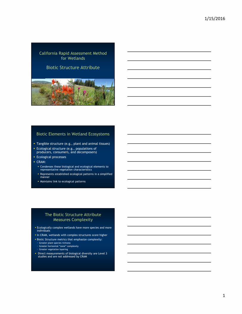
Ground nesting birds require vegetation cover at nest sites

Plant canopies entrap coarse plant litter that is lifted into the canopies by rising water (tides or floods)

This “entrained” material is left hanging in the plant cover, providing shelter for birds and small mammals

Entrained Vegetation Functions

Dense Canopy Functions

Rainfall interception

Reduced evaporation from soils

Enhanced filtration of flood waters

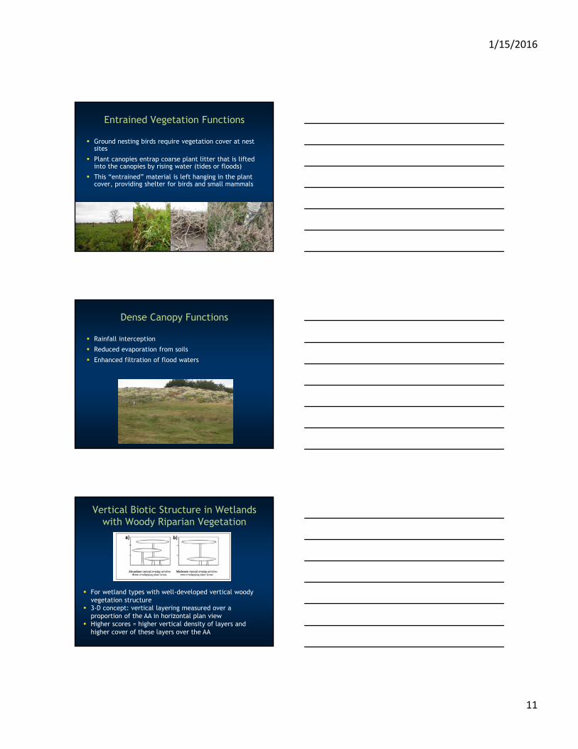
Vertical Biotic Structure in Wetlands with Woody Riparian Vegetation

For wetland types with well-developed vertical woody vegetation structure

3-D concept: vertical layering measured over a proportion of the AA in horizontal plan view

Higher scores = higher vertical density of layers and higher cover of these layers over the AA

1/15/2016

12

Rating Alternative States

AMore than 50% of the vegetated area of the AA supports abundantoverlap of 3 plant layers.

B More than 50% of the vegetated area of the AA supports at least moderate overlap of 2 plant layers.

C25%-50% of the vegetated area of the AA supports at leastmoderate overlap of 2 plant layers.

DLess than 25% of the vegetated area of the AA supports moderateoverlap of 2 plant layers OR AA is sparsely vegetated overall.

Vertical Biotic StructureScoring Using Overlap

Moderate Overlap (2 layers)

Abundant Overlap (3 layers)

1/15/2016

13

Vertical Biotic Structure in Emergent Wetlands with Herbaceous Vegetation

Values and functions of entrained litter in herbaceous wetlands

Estuarine and depressionalwetlands

Proportion of AA with entrained litter

Rating Alternative States

A

Most of the vegetated plain of the AA has a dense canopy of living vegetation or entrained litter or detritus forming a “ceiling” of cover above the wetland surface that shades the surface and can provide abundant cover for wildlife.

B

Less than half (25-50%) of the vegetated plain of the AA has a dense canopy of vegetation or entrained litter or detritus as described in “A” above;ORMost of the vegetated plain has a sparse canopy of vegetation or entrained litter or detritus.

C25-50% of the vegetated plain of the AA has a sparse canopy of vegetation or entrained litter or detritus.

DMost of the AA (>75%) lacks a canopy of living vegetation or entrained litter or detritus.

Vertical Biotic StructureScoring Using Entrainment

Vertical Biotic Structure in Emergent Wetlands with Woody Riparian Elements

Many wetlands have both marshy emergent layers and woody “riparian” vegetation

Higher scores = higher vertical density of layers and higher cover of these layers over the AA