14

THE EcosysTEm

2.1 Structure

2

Assessment statements2.1.1 Distinguish between biotic and abiotic (physical) components of an ecosystem.2.1.2 Define the term trophic level. 2.1.3 Identify and explain trophic levels in food chains and food webs selected from

the local environment.2.1.4 Explain the principles of pyramids of numbers, pyramids of biomass, and

pyramids of productivity, and construct such pyramids from given data.2.1.5 Discuss how the pyramid structure affects the functioning of an ecosystem.2.1.6 Define the terms species, population, habitat, niche, community and

ecosystem with reference to local examples.2.1.7 Describe and explain population interactions using examples of named

species.

Biotic and abiotic components

Biotic refers to the living components within an ecosystem (the community). Abiotic refers to the non-living factors of the ecosystem (the environment).

Ecosystems consist of living and non-living components. Organisms (animals, plants, algae, fungi and bacteria) are the organic or living part of the ecosystem. The physical environment (light, air, water, temperature, minerals, soil and climatic aspects) constitute the non-living part. The living parts of an ecosystem are called the biotic components and the non-living parts the abiotic (not biotic) components. Abiotic factors include the soil (edaphic factors) and topography (the landscape). Biotic and non-biotic components interact to sustain the ecosystem. The word ‘environment’ refers specifically to the non-living part of the ecosystem.

To find links to hundreds of environmental sites, go to www.pearsonhotlinks.com, insert the express code 2630P and click on activity 2.1.

To learn more about all things environmental, go to www.pearsonhotlinks.com, insert the express code 2630P and click on activity 2.2.

Trophic levels, food chains and food websCertain organisms in an ecosystem convert abiotic components into living matter. These are the producers; they support the ecosystem by producing new biological matter (biomass) (Figure 2.1). Organisms that cannot make their own food eat other organisms to obtain energy and matter. They are consumers. The flow of energy and matter from organism to organism can be shown in a food chain. The position that an organism occupies in a food chain is called the trophic level (Figure 2.2). Trophic level can also mean the position in the food chain occupied by a group of organisms in a community.

The term ‘trophic level’ refers to the feeding level within a food chain. Food webs are made from many interconnecting food chains.

02_M02_14_82.indd 14 15/04/2010 08:53

1515

some light is reflected

solar energy

some light is transmitted

some wavelengths are unsuitable

photosynthesis changes solar energy to chemical energy

biomass stores energy

energy lost through respiration

producer primaryconsumer

secondary consumer

tertiaryconsumer

quaternary consumer

autotroph herbivore omnivore/carnivore carnivore carnivore

Ecosystems contain many interconnected food chains that form food webs. There are a variety of ways of showing food webs, and they may include decomposers which feed on the dead biomass created by the ecosystem (Figure 2.3). The producer in this food web for the North Sea is phytoplankton (microscopic algae), the primary consumers (herbivores) are zooplankton (microscopic animal life), the secondary consumers (carnivores) include jellyfish, sand eels, and herring (each on different food chains), and the tertiary consumers (top carnivores) are mackerel, seals, seabirds and dolphins (again on different food chains).

sea surface

solar energy puffins, gannets

light available forphotosynthesis

dolphins

herring

squid

crustaceans feed on decaying organic material

cod, haddock

continental shelf

sea bed

phytoplankton usedisolved nutrientsand carbon dioxideto photosynthesise

zooplankton seals

mackerel sand eels jellyfish

Diagrams of food webs can be used to estimate knock-on effects of changes to the ecosystem. During the 1970s, sand eels were harvested and used as animal feed, for fishmeal and for oil and food on salmon farms: Figure 2.3 can be used to explain what impacts a

Figure 2.1Producers covert sunlight energy into chemical energy using photosynthetic pigments. The food produced supports the rest of the food chain.

Figure 2.2A food chain. Ecosystems contain many food chains.

Figure 2.3A simplified food web for the North Sea in Europe.

02_M02_14_82.indd 15 15/04/2010 08:53

16

THE ECOSYSTEM2

dramatic reduction in the number of sand eels might have on the rest of the ecosystem. Sand eels are the only source of food for mackerel, puffin and gannet, so numbers of these species may decline or they may have to switch food source. Similarly, seals will have to rely more on herring, possibly reducing their numbers or they may also have to switch food source. The amount of zooplankton may increase, improving food supply for jellyfish and herring.

An estimated 1000 kg of plant plankton are needed to produce 100 kg of animal plankton. The animal plankton is in turn consumed by 10 kg of fish, which is the amount needed by a person to gain 1 kg of body mass. Biomass and energy decline at each successive trophic level so there is a limit to the number of trophic levels which can be supported in an ecosystem. Energy is lost as heat (produced as a waste product of respiration) at each stage in the food chain, so only energy stored in biomass is passed on to the next trophic level. Thus, after 4 or 5 trophic stages, there is not enough energy to support another stage.

The earliest forms of life on Earth, 3.8 billion years ago, were consumers feeding on organic material formed by interactions between the atmosphere and the land surface. Producers appeared around 3 billion years ago – these were photosynthetic bacteria and their photosynthesis led to a dramatic increase in the amount of oxygen in the atmosphere. The oxygen enabled organisms that used aerobic respiration to generate the large amounts of energy they needed. And, eventually, complex ecosystems followed.

Pyramids of numbers, biomass and productivityPyramids are graphical models of the quantitative differences that exist between the trophic levels of a single ecosystem. These models provide a better understanding of the workings of an ecosystem by showing the feeding relationship in a community.

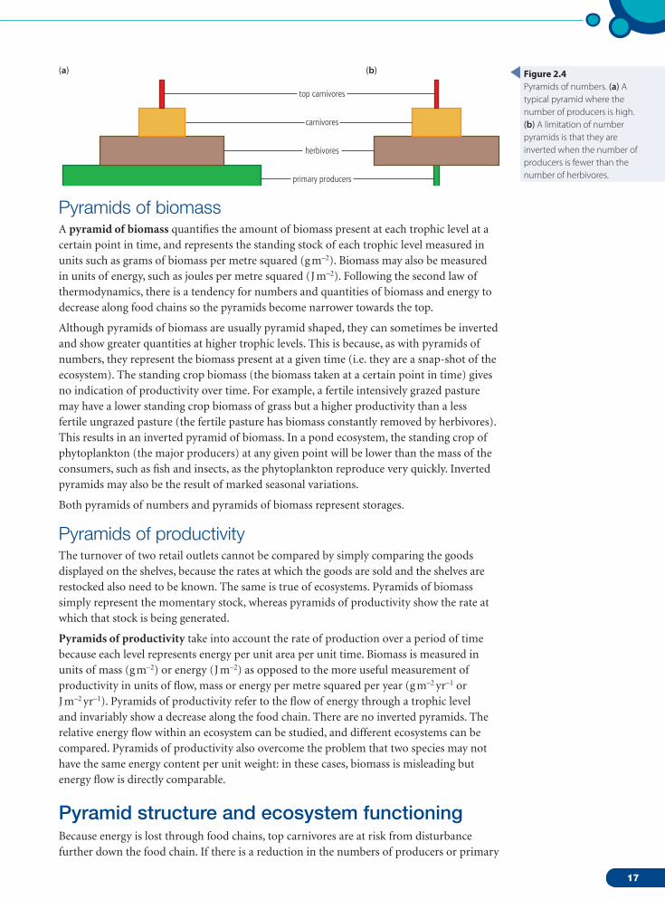
Pyramids of numbersThe numbers of producers and consumers coexisting in an ecosystem can be shown by counting the numbers of organisms in an ecosystem and constructing a pyramid. Quantitative data for each trophic level are drawn to scale as horizontal bars arranged symmetrically around a central axis (Figure 2.4a). Sometimes, rather than counting every individual in a trophic level, limited collections may be done in a specific area and this multiplied up to the total area of the ecosystem. Pyramids of numbers are not always pyramid shaped; for example, in a woodland ecosystem with many insect herbivores feeding on trees, there are bound to be fewer trees than insects; this means the pyramid is inverted (upside-down) as in Figure 2.4b. This situation arises when the size of individuals at lower trophic levels are relatively large. Pyramids of numbers, therefore, have limitations in showing useful feeding relationships.

Examiner’s hint:You will need to find an example of a food chain from your local area, with named examples of producers, consumers, decomposers, herbivores, carnivores, and top carnivores.

Food chains always begin with the producers (usually photosynthetic organisms), followed by primary consumers (herbivores), secondary consumers (omnivores or carnivores) and then higher consumers (tertiary, quaternary, etc.). Decomposers feed at every level of the food chain.

Pyramids are graphical models showing the quantitative differences between the tropic levels of an ecosystem. There are three types.•Pyramid of numbers

– This records the number of individuals at each trophic level.

•Pyramid of biomass – This represents the biological mass of the standing stock at each trophic level at a particular point in time.

•Pyramid of productivity – This shows the flow of energy (i.e. the rate at which the stock is being generated) through each trophic level.

Stromatolites were the earliest producers on the planet and are still here. These large aggregations of cyanobacteria can be found in the fossil record and alive in locations such as Western Australia and Brazil.

02_M02_14_82.indd 16 15/04/2010 08:54

171717

top carnivores

(a) (b)

carnivores

herbivores

primary producers

Pyramids of biomassA pyramid of biomass quantifies the amount of biomass present at each trophic level at a certain point in time, and represents the standing stock of each trophic level measured in units such as grams of biomass per metre squared (g m–2). Biomass may also be measured in units of energy, such as joules per metre squared (J m–2). Following the second law of thermodynamics, there is a tendency for numbers and quantities of biomass and energy to decrease along food chains so the pyramids become narrower towards the top.

Although pyramids of biomass are usually pyramid shaped, they can sometimes be inverted and show greater quantities at higher trophic levels. This is because, as with pyramids of numbers, they represent the biomass present at a given time (i.e. they are a snap-shot of the ecosystem). The standing crop biomass (the biomass taken at a certain point in time) gives no indication of productivity over time. For example, a fertile intensively grazed pasture may have a lower standing crop biomass of grass but a higher productivity than a less fertile ungrazed pasture (the fertile pasture has biomass constantly removed by herbivores). This results in an inverted pyramid of biomass. In a pond ecosystem, the standing crop of phytoplankton (the major producers) at any given point will be lower than the mass of the consumers, such as fish and insects, as the phytoplankton reproduce very quickly. Inverted pyramids may also be the result of marked seasonal variations.

Both pyramids of numbers and pyramids of biomass represent storages.

Pyramids of productivityThe turnover of two retail outlets cannot be compared by simply comparing the goods displayed on the shelves, because the rates at which the goods are sold and the shelves are restocked also need to be known. The same is true of ecosystems. Pyramids of biomass simply represent the momentary stock, whereas pyramids of productivity show the rate at which that stock is being generated.

Pyramids of productivity take into account the rate of production over a period of time because each level represents energy per unit area per unit time. Biomass is measured in units of mass (g m–2) or energy (J m–2) as opposed to the more useful measurement of productivity in units of flow, mass or energy per metre squared per year (g m–2 yr–1 or J m–2 yr–1). Pyramids of productivity refer to the flow of energy through a trophic level and invariably show a decrease along the food chain. There are no inverted pyramids. The relative energy flow within an ecosystem can be studied, and different ecosystems can be compared. Pyramids of productivity also overcome the problem that two species may not have the same energy content per unit weight: in these cases, biomass is misleading but energy flow is directly comparable.

Pyramid structure and ecosystem functioningBecause energy is lost through food chains, top carnivores are at risk from disturbance further down the food chain. If there is a reduction in the numbers of producers or primary

Figure 2.4Pyramids of numbers. (a) A typical pyramid where the number of producers is high. (b) A limitation of number pyramids is that they are inverted when the number of producers is fewer than the number of herbivores.

(a) (b)

02_M02_14_82.indd 17 15/04/2010 08:54

18

THE ECOSYSTEM2

consumers, existence of the top carnivores can be put at risk if there are not enough organisms (and therefore energy and biomass) to support them. Top carnivores may be the first population to noticeably suffer through ecosystem disruption.

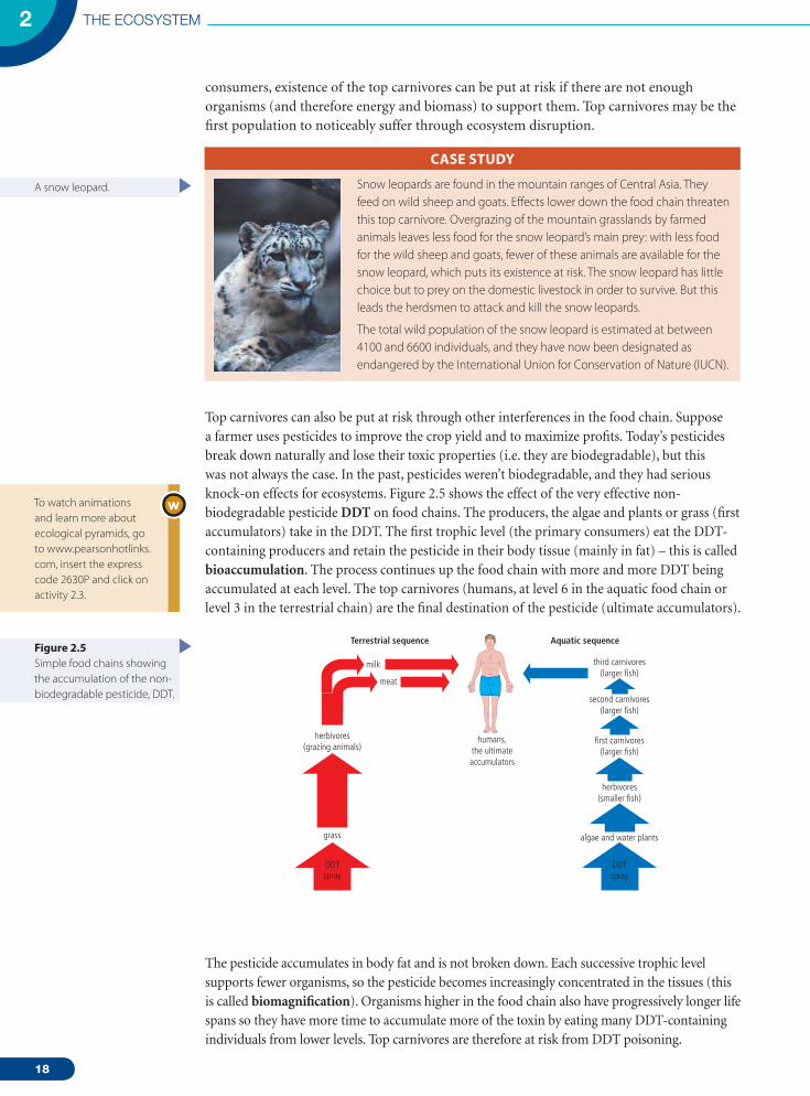
Top carnivores can also be put at risk through other interferences in the food chain. Suppose a farmer uses pesticides to improve the crop yield and to maximize profits. Today’s pesticides break down naturally and lose their toxic properties (i.e. they are biodegradable), but this was not always the case. In the past, pesticides weren’t biodegradable, and they had serious knock-on effects for ecosystems. Figure 2.5 shows the effect of the very effective non-biodegradable pesticide DDT on food chains. The producers, the algae and plants or grass (first accumulators) take in the DDT. The first trophic level (the primary consumers) eat the DDT-containing producers and retain the pesticide in their body tissue (mainly in fat) – this is called bioaccumulation. The process continues up the food chain with more and more DDT being accumulated at each level. The top carnivores (humans, at level 6 in the aquatic food chain or level 3 in the terrestrial chain) are the final destination of the pesticide (ultimate accumulators).

Terrestrial sequence

meat

milk

Aquatic sequence

DDT spray

DDT spray

algae and water plants

herbivores (smaller fish)

first carnivores (larger fish)

second carnivores (larger fish)

third carnivores (larger fish)

grass

herbivores (grazing animals)

humans, the ultimate accumulators

The pesticide accumulates in body fat and is not broken down. Each successive trophic level supports fewer organisms, so the pesticide becomes increasingly concentrated in the tissues (this is called biomagnification). Organisms higher in the food chain also have progressively longer life spans so they have more time to accumulate more of the toxin by eating many DDT-containing individuals from lower levels. Top carnivores are therefore at risk from DDT poisoning.

To watch animations and learn more about ecological pyramids, go to www.pearsonhotlinks.com, insert the express code 2630P and click on activity 2.3.

Figure 2.5Simple food chains showing the accumulation of the non-biodegradable pesticide, DDT.

A snow leopard.

CasE study

Snow leopards are found in the mountain ranges of Central Asia. They feed on wild sheep and goats. Effects lower down the food chain threaten this top carnivore. Overgrazing of the mountain grasslands by farmed animals leaves less food for the snow leopard’s main prey: with less food for the wild sheep and goats, fewer of these animals are available for the snow leopard, which puts its existence at risk. The snow leopard has little choice but to prey on the domestic livestock in order to survive. But this leads the herdsmen to attack and kill the snow leopards.

The total wild population of the snow leopard is estimated at between 4100 and 6600 individuals, and they have now been designated as endangered by the International Union for Conservation of Nature (IUCN).

02_M02_14_82.indd 18 15/04/2010 08:54

19

EXERCIsEs

1

2

3

4

5

Distinguish between biotic and abiotic factors. Which of these terms refers to the environment of an ecosystem?

What are the differences between a pyramid of biomass and a pyramid of productivity? Which is always pyramid shaped, and why? Give the units for each type of pyramid.

How can total biomass be calculated?

Why are non-biodegradable toxins a hazard to top predators in a food chain?

Why are food chains short (i.e. generally no more than five trophic levels in length)? What are the implications of this for the conservation of top carnivores?

Species, populations, habitats and nichesEcological terms are precisely defined and may vary from the everyday use of the same words. Definitions for key terms are given below.

SpeciesA species is defined as a group of organisms that interbreed and produce fertile offspring. If two species breed together to produce a hybrid, this may survive to adulthood but cannot produce viable gametes and so is sterile. An example of this is when a horse (Equus caballus) breeds with a donkey (Equus asinus) to produce a sterile mule.

The species concept cannot:• identify whether geographically isolated populations belong to the same species• classify species in extinct populations• account for asexually reproducing organisms• clearly define species when barriers to reproduction are incomplete (Figure 2.6).

Vega herring gull

herring gull

American herring gull

Birula’s gull

Heuglin’s gull

Siberian lesser black-backed gull

lesser black-backed gull

PopulationA population is defined in ecology as a group of organisms of the same species living in the same area at the same time, and which are capable of interbreeding.

Examiner’s hint:• A pyramid of biomass

represents biomass (standing stock) at a given time, whereas a pyramid of productivity represents the rate at which stocks are being generated (i.e. the flow of energy through the food chain). A pyramid of biomass is measured in units of mass (g m–2) or energy (J m–2); a pyramid of productivity is measured in units of flow (g m–2 yr–1 or J m–2 yr–1).

• Because energy is lost through the food chain, pyramids of productivity are always pyramid shaped. Pyramids of number or biomass may be inverted because they represent only the stock at a given moment in time.

Figure 2.6 Gulls interbreeding in a ring around the Arctic are an example of ring species. Neighbouring species can interbreed to produce viable hybrids but herring gulls and lesser black-backed gulls, at the ends of the ring, cannot interbreed.

The species concept is sometimes difficult to apply: for example, can it be used accurately to describe extinct animals and fossils? The term is also sometimes loosely applied to what are, in reality, sub-species that can interbreed. This is an example of an apparently simple term that is difficult to apply in practical situations.

02_M02_14_82.indd 19 15/04/2010 08:54

20

THE ECOSYSTEM2

HabitatHabitat refers to the environment in which a species normally lives. For example, the habitat of wildebeest is the savannah and temperate grasslands of eastern and south-eastern Africa.

NicheAn ecological niche is best be described as where, when and how an organism lives. An organism’s niche depends not only on where it lives (its habitat) but also on what it does. For example, the niche of a zebra includes all the information about what defines this species: its habitat, courtship displays, grooming, alertness at water holes, when it is active, interactions between predators and similar activities. No two different species can have the same niche because the niche completely defines a species.

CommunityA community is a group of populations living and interacting with each other in a common habitat. This contrasts with the term ‘population’ which refers to just one species. The grasslands of Africa contain wildebeest, lions, hyenas, giraffes and elephants as well as zebras. Communities include all biotic parts of the ecosystem, both plants and animals.

EcosystemAn ecosystem is a community of interdependent organisms (the biotic component) and the physical environment (the abiotic component) they inhabit.

A population of zebras.

Wildebeest in their habitat.

• Species – A group of organisms that interbreed and produce fertile offspring.

• Population – A group of organisms of the same species living in the same area at the same time, and which are capable of interbreeding.

• Habitat – The environment in which a species normally lives.

• Niche – Where and how a species lives. A species’ share of a habitat and the resources in it.

• Community – A group of populations living and interacting with each other in a common habitat.

• Ecosystem – A community of interdependent organisms and the physical environment they inhabit.

To access worksheet 2.1 on mini-ecosystems, please visit www.pearsonbacconline.com and follow the on-screen instructions.

02_M02_14_82.indd 20 15/04/2010 08:54

21

Population interactionsEcosystems contain numerous populations with complex interactions between them. The nature of the interactions varies and can be broadly divided into four types (competition, predation, parasitism and mutualism), each of which is discussed below.

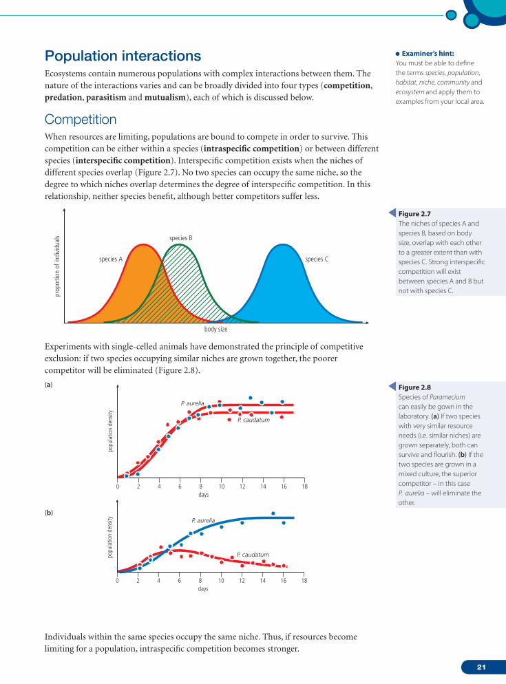
CompetitionWhen resources are limiting, populations are bound to compete in order to survive. This competition can be either within a species (intraspecific competition) or between different species (interspecific competition). Interspecific competition exists when the niches of different species overlap (Figure 2.7). No two species can occupy the same niche, so the degree to which niches overlap determines the degree of interspecific competition. In this relationship, neither species benefit, although better competitors suffer less.

prop

ortio

n of

indi

vidu

als

body size

species A species C

species B

Experiments with single-celled animals have demonstrated the principle of competitive exclusion: if two species occupying similar niches are grown together, the poorer competitor will be eliminated (Figure 2.8).

days10 12 14 16 186

(a)

(b)

8420

popu

latio

n de

nsity P. aurelia

P. caudatum

days10 12 14 16 186 8420

popu

latio

n de

nsity

P. aurelia

P. caudatum

days10 12 14 16 186

(a)

(b)

8420

popu

latio

n de

nsity P. aurelia

P. caudatum

days10 12 14 16 186 8420

popu

latio

n de

nsity

P. aurelia

P. caudatum

Individuals within the same species occupy the same niche. Thus, if resources become limiting for a population, intraspecific competition becomes stronger.

Examiner’s hint:You must be able to define the terms species, population, habitat, niche, community and ecosystem and apply them to examples from your local area.

Figure 2.8Species of Paramecium can easily be gown in the laboratory. (a) If two species with very similar resource needs (i.e. similar niches) are grown separately, both can survive and flourish. (b) If the two species are grown in a mixed culture, the superior competitor – in this case P. aurelia – will eliminate the other.

Figure 2.7The niches of species A and species B, based on body size, overlap with each other to a greater extent than with species C. Strong interspecific competition will exist between species A and B but not with species C.

(a)

(b)

02_M02_14_82.indd 21 15/04/2010 08:54

22

THE ECOSYSTEM2

PredationPredation occurs when one animal (or, occasionally, a plant) hunts and eats another animal. These predator–prey interactions are often controlled by negative feedback mechanisms that control population densities (e.g. the snowshoe hare and lynx, page 8).

ParasitismIn this relationship, one organism (the parasite) benefits at the expense of another (the host) from which it derives food. Ectoparasites live on the surface of their host (e.g. ticks and mites); endoparasites live inside their host (e.g. tapeworms). Some plant parasites draw food from the host via their roots.

MutualismSymbiosis is a relationship in which two organisms live together (parasitism is a form of symbiosis where one of the organisms is harmed). Mutualism is a symbiotic relationship in which both species benefit. Examples include coral reefs and lichens. Coral reefs show a symbiotic relationship between the coral animal (polyp) and zooxanthellae (unicellular brown algae or dinoflagellates) that live within the coral polyp (Figure 2.9).

Nepenthes rajah, the largest pitcher plant, can hold up to 3.5 litres of water in the pitcher and has been known to trap and digest small mammals such as rats. Nepenthes rajah is endemic to Mount Kinabalu where it lives between 1500 and 2650 m above sea level (pages 66–67).

Rafflesia have the largest flowers in the world but no leaves. Without leaves, they cannot photosynthesize, so they grow close by South-East Asian vines (Tetrastigma spp.) from which they draw the sugars they need for growth.

Not all predators are animals. Insectivorous plants, such as the Venus fly traps and pitcher plants trap insects and feed on them. Such plants often live in areas with nitrate-poor soils and obtain much of their nitrogen from animal protein.

02_M02_14_82.indd 22 15/04/2010 08:54

23

tenticles with nematocysts (stinging cells)

living tissue linking polyps

skeleton

zooxanthellae

nematocyst

gastrovascular cavity (digestive sac)

limestone calice

mouth

EXERCIsEs

1

2

3

Define the terms species, population, habitat, niche, community, and ecosystem. What is the difference between a habitat and a niche? Can different species occupy the same niche?

What is the difference between mutualism and parasitism? Give examples of each.

The abundance of one species can affect the abundance of another. Give an ecological example of this, and explain how the predator affects the abundance of the prey, and vice versa. Are population numbers generally constant in nature? If not, what implications does this have for the measurement of wild population numbers?

Figure 2.9The zooxanthellae living within the polyp animal photosynthesize to produce food for themselves and the coral polyp, and in return are protected.

Lichens consist of a fungus and alga in a symbiotic relationship. The fungus is efficient at absorbing water but cannot photosynthesize, whereas the alga contains photosynthetic pigments and so can use sunlight energy to convert carbon dioxide and water into glucose. The alga therefore obtains water and shelter, and the fungus obtains a source of sugar from the relationship. Lichens with different colours contain algae with different photosynthetic pigments.

Mutualism is a symbiotic relationship in which both species benefit.

Parasitism is a symbiotic relationship in which one species benefits at the expense of the other.

02_M02_14_82.indd 23 15/04/2010 08:54

24

THE ECOSYSTEM2

2.2 Measuring abiotic components of the system

Assessment statements2.2.1 List the significant abiotic (physical) factors of an ecosystem.2.2.2 Describe and evaluate methods for measuring at least three abiotic (physical)

factors within an ecosystem.

Measuring abiotic componentsEcosystems can be broadly divided into three types.• Marine – The sea, estuaries, salt marshes and mangroves are all characterized by the high

salt content of the water.• Freshwater – Rivers, lakes and wetlands.• Terrestrial – Land-based.

Each ecosystem has its own specific abiotic factors (listed below) as well as the ones they share.

Abiotic factors of a marine ecosystem:• salinity• pH• temperature• dissolved oxygen• wave action.

Estuaries are classified as marine ecosystems because they have high salt content compared to freshwater. Mixing of freshwater and oceanic sea water leads to diluted salt content but it is still high enough to influence the distribution of organisms within it – salt-tolerant animals and plants have specific adaptations to help them cope with the osmotic demands of saltwater.

Only a small proportion of freshwater is found in ecosystems (Figure 2.10). Abiotic factors of a freshwater ecosystem:• turbidity • temperature• flow velocity • dissolved oxygen• pH.

ice and snow68.7%

fresh groundwater30.1%

permafrost0.86%

lakes0.26% soil moisture 0.05%

wetlands 0.03%

rivers0.006%

Figure 2.10The majority of the Earth’s freshwater is locked up in ice and snow, and is not directly available to support life. Groundwater is a store of water beneath ground and again is inaccessible for living organisms.

02_M02_14_82.indd 24 15/04/2010 08:54

25

Abiotic factors of a terrestrial ecosystem:• temperature• light intensity• wind speed• particle size• slope/aspect• soil moisture• drainage• mineral content.

You must know methods for measuring each of the abiotic factors listed above and how they might vary in any given ecosystem with depth, time or distance. Abiotic factors are examined in conjunction with related biotic components (pages 29–34). This allows species distribution data to be linked to the environment in which they are found and explanations for the patterns to be proposed.

Distribution of Earth’s water

fresh water3%

other0.9%

rivers2%

swamps11%

lakes87%

groundwater30.1%

surfacewater0.3%

icecaps andglaciers68.7%

saltwater97%

fresh surface water fresh water Earth’s water

The Nevada desert, USA. Water supply in terrestrial ecosystems can be extremely limited, especially in desert areas, and is an important abiotic factor in controlling the distribution of organisms.

To learn more about sampling techniques, go to www.pearson.co.uk, insert the express code 2630P and click on activity 2.4.

The majority of the Earth’s water is found in the oceans, with relatively little in lakes and rivers. Much of the freshwater that does exist is stored in ice at the poles (Figures 2.10 and 2.11).

Figure 2.11The percentage of the planet containing freshwater ecosystems is extremely low compared to oceanic ones.

02_M02_14_82.indd 25 15/04/2010 08:55

26

THE ECOSYSTEM2

Evaluating measures for describing abiotic factorsThis section examines the techniques used for measuring abiotic factors. An inaccurate picture of an environment may be obtained if errors are made in sampling: possible sources of error are examined below.

LightA light-meter can be used to measure the light in an ecosystem. It should be held at a standard and fixed height above the ground and read when the value is fixed and not fluctuating. Cloud cover and changes in light intensity during the day mean that values must be taken at the same time of day and same atmospheric conditions: this can be difficult if several repeats are taken. The direction of the light-meter also needs to be standardized so it points in the same direction at the same angle each time it is used. Care must be taken not to shade the light-meter during a reading.

TemperatureOrdinary mercury thermometers are too fragile for fieldwork, and are hard to read. An electronic thermometer with probes (datalogger) allows temperature to be measured in air, water, and at different depths in soil. The temperature needs to be taken at a standard depth. Problems arise if the thermometer is not buried deeply enough: the depth needs to be checked each time it is used.

pHThis can be measured using a pH meter or datalogging pH probe. Values in freshwater range from slightly basic to slightly acidic depending on surrounding soil, rock and vegetation. Sea water usually has a pH above 7 (alkaline). The meter or probe must be cleaned between each reading and the reading taken from the same depth. Soil pH can be measured using a soil test kit – indicator solution is added and the colour compared to a chart.

WindMeasurements can be taken by observing the effects of wind on objects – these are then related to the Beaufort scale. Precise measurements of wind speed can be made with a digital anemometer. The device can be mounted or hand-held. Some use cups to capture the wind whereas other smaller devices use a propeller. Care must be taken not to block the wind. Gusty conditions may lead to large variations in data.

Particle sizeSoil can be made up of large, small or intermediate particles. Particle size determines drainage and water-holding capacity (page 125). Large particles (pebbles) can be measured individually and the average particle size calculated. Smaller particles can be measured by using a series of sieves with increasingly fine mesh size. The smallest particles can be separated by sedimentation. Optical techniques (examining the properties of light scattered by a suspension of soil in water) can also be used to study the smallest particles. The best techniques are expensive and the simpler ones time consuming.

Abiotic factors that can be measured within an ecosystem include the following.• Marine environment

– Salinity, pH, temperature, dissolved oxygen, wave action.

• Freshwater environment – Turbidity, flow velocity, pH, temperature, dissolved oxygen.

• Terrestrial environment – Temperature, light intensity, wind speed, particle size, slope, soil moisture, drainage, mineral content.

An anemometer measuring wind speed. It works by converting the number of rotations made by three cups at the top of the apparatus into wind speed.

02_M02_14_82.indd 26 15/04/2010 08:55

27

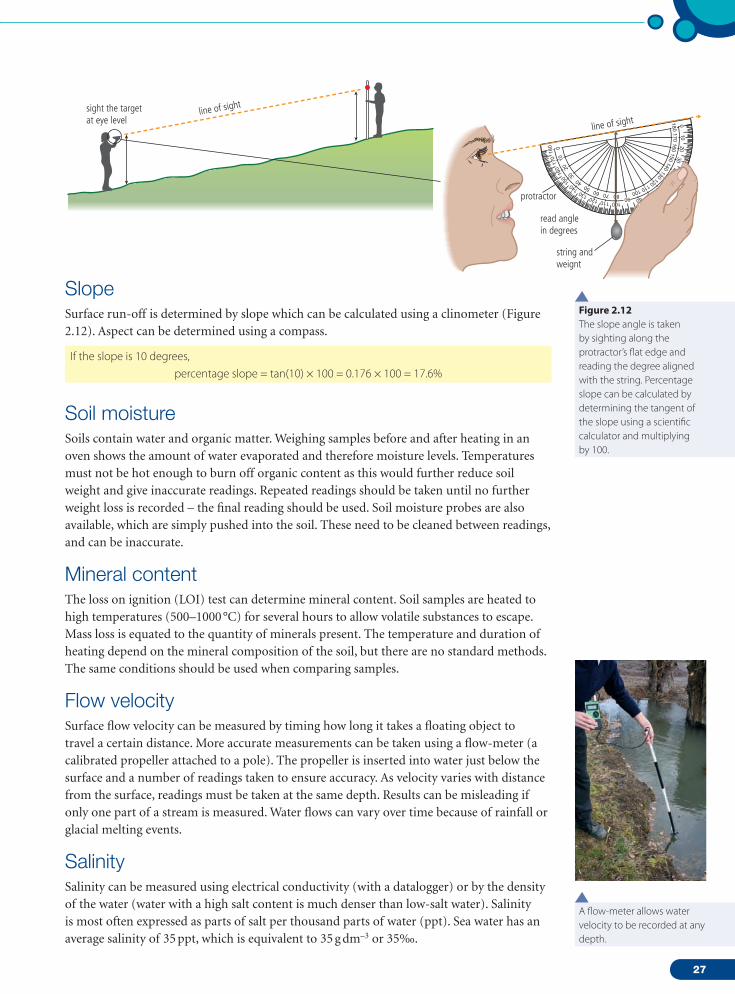
SlopeSurface run-off is determined by slope which can be calculated using a clinometer (Figure 2.12). Aspect can be determined using a compass.

If the slope is 10 degrees,

percentage slope = tan(10) × 100 = 0.176 × 100 = 17.6%

Soil moistureSoils contain water and organic matter. Weighing samples before and after heating in an oven shows the amount of water evaporated and therefore moisture levels. Temperatures must not be hot enough to burn off organic content as this would further reduce soil weight and give inaccurate readings. Repeated readings should be taken until no further weight loss is recorded – the final reading should be used. Soil moisture probes are also available, which are simply pushed into the soil. These need to be cleaned between readings, and can be inaccurate.

Mineral contentThe loss on ignition (LOI) test can determine mineral content. Soil samples are heated to high temperatures (500–1000 °C) for several hours to allow volatile substances to escape. Mass loss is equated to the quantity of minerals present. The temperature and duration of heating depend on the mineral composition of the soil, but there are no standard methods. The same conditions should be used when comparing samples.

Flow velocitySurface flow velocity can be measured by timing how long it takes a floating object to travel a certain distance. More accurate measurements can be taken using a flow-meter (a calibrated propeller attached to a pole). The propeller is inserted into water just below the surface and a number of readings taken to ensure accuracy. As velocity varies with distance from the surface, readings must be taken at the same depth. Results can be misleading if only one part of a stream is measured. Water flows can vary over time because of rainfall or glacial melting events.

SalinitySalinity can be measured using electrical conductivity (with a datalogger) or by the density of the water (water with a high salt content is much denser than low-salt water). Salinity is most often expressed as parts of salt per thousand parts of water (ppt). Sea water has an average salinity of 35 ppt, which is equivalent to 35 g dm–3 or 35‰.

A flow-meter allows water velocity to be recorded at any depth.

Figure 2.12The slope angle is taken by sighting along the protractor’s flat edge and reading the degree aligned with the string. Percentage slope can be calculated by determining the tangent of the slope using a scientific calculator and multiplying by 100.

line of sight

protractor

read anglein degrees

line of sight sight the target at eye level

string andweignt

02_M02_14_82.indd 27 15/04/2010 08:55

28

THE ECOSYSTEM2

Dissolved oxygenOxygen-sensitive electrodes connected to a meter can be used to measure dissolved oxygen. Care must be taken when using an oxygen meter to avoid contamination from oxygen in the air. A more labour-intensive method is Winkler titration – this is based on the principle that oxygen in the water reacts with iodide ions, and acid can then added to release iodine that can be quantitatively measured.

Wave actionAreas with high wave action have high levels of dissolved oxygen due to mixing of air and water in the turbulence. Wave action is measured using a dynamometer, which measures the force in the waves. Changes in tide and wave strength during the day and over monthly periods mean that average results must be used to take this variability into account.

TurbidityCloudy water is said to have high turbidity and clear water low turbidity. Turbidity affects the penetration of sunlight into water and therefore rates of photosynthesis. Turbidity can be measured using a Secchi disc (Figure 2.13). Problems may be caused by the Sun’s glare on the water, or the subjective nature of the measure with one person seeing the disc at one depth but another, with better eyesight, seeing it at a greater depth. Errors can be avoided by taking measures on the shady side of a boat.

More sophisticated optical devices can also be used (e.g. a nephelometer or turbidimeter) to measure the intensity of light scattered at 90° as a beam of light passes through a water sample.

Evaluation of techniquesShort-term and limited field sampling reduces the effectiveness of the above techniques because abiotic factors may vary from day to day and season to season. The majority of these abiotic factors can be measured using datalogging devices. The advantage of dataloggers is that they can provide continuous data over a long period of time, making results more representative of the area. As always, the results can be made more reliable by taking many samples.

Abiotic data can be collected using instruments that avoid issues of objectivity as they directly record quantitative data. Instruments allow us to record data that would otherwise be beyond the limit of our perception.

EXERCIsEs

1

2

3

List as many abiotic factors as you can think of. Say how you would measure each of these factors in an ecological investigation.

Evaluate each of the methods you have listed in exercise 1. What are their limitations, and how may they affect the data you collect?

Which methods could you use in (a) marine ecosystems, (b) freshwater ecosystems and (c) terrestrial ecosystems?

Assessment statements2.3.1 Construct simple keys and use published keys for the identification of

organisms.2.3.2 Describe and evaluate methods for estimating abundance of organisms.2.3.3 Describe and evaluate methods for estimating the biomass of trophic levels in a

community.2.3.4 Define the term diversity. 2.3.5 Apply Simpson’s diversity index and outline its significance.

Figure 2.13A Secchi disc is mounted on a pole or line and is lowered into water until it is just out of sight. The depth is measured using the scale of the line or pole. The disc is raised until it is just visible again and a second reading is taken. The average depth calculated is known as the Secchi depth.

02_M02_14_82.indd 28 15/04/2010 08:55

29

2.3 Measuring biotic components of the system

Assessment statements2.3.1 Construct simple keys and use published keys for the identification of

organisms.2.3.2 Describe and evaluate methods for estimating abundance of organisms.2.3.3 Describe and evaluate methods for estimating the biomass of trophic levels in a

community.2.3.4 Define the term diversity. 2.3.5 Apply Simpson’s diversity index and outline its significance.

Keys for species identificationEcology is the study of living organisms in relation to their environment. We have examined the abiotic environmental factors that need to be studied, now we will look at the biotic or living factors. In any ecological study, it is important to correctly identify the organisms in question otherwise results and conclusions will be invalid. It is unlikely that you will be an expert in the animals or plants you are looking at, so you will need to use dichotomous keys.

Dichotomous means ‘divided into two parts’. The key is written so that identification is done in steps. At each step, two options are given based on different possible characteristics of the organism you are looking at. The outcome of each choice leads to another pair of questions, and so on until the organism is identified.

For example, suppose you were asked to create a dichotomous key based on the following list of specimens: rat, shark, buttercup, spoon, amoeba, sycamore tree, pebble, pine tree, eagle, beetle, horse, and car. An example of a suitable key is given below.

1 a Organism is living go to 4b Organism is non-living go to 2

2 a Object is metallic go to 3b Object is non-metallic pebble

3 a Object has wheels carb Object does not have wheels spoon

4 a Organism is microscopic amoebab Organism is macroscopic go to 5

5 a Organism is a plant go to 6b Organism is an animal go to 8

6 a Plant has a woody stem go to 7b Plant has a herbaceous stem buttercup

7 a Tree has leaves with small surface area pine treeb Tree has leaves with large surface area sycamore tree

8 a Organism is terrestrial go to 9b Organism is aquatic shark

9 a Organism has fewer than 6 legs go to 10b Organism has 6 legs beetle

10 a Organism has fur go to 11b Organism has feathers eagle

11 a Organism has hooves horseb Organism has no hooves rat

The key can also be shown graphically (Figure 2.14, overleaf).

02_M02_14_82.indd 29 15/04/2010 08:55

30

THE ECOSYSTEM2

living

macroscopic microscopic

amoeba

terrestrial

feathers

eagle

fur

hooves

horse

without hooves

rat

aquatic

shark

animal plant

non-living

metallicnon-metallic

pebble wheels no wheels

car spoon woody stem

herbaceous

buttercup

6 legs

beetle

leaves with small surface area

leaves with large surface area

pine tree sycamore tree

fewer than 6 legs

Describe and evaluate methods for estimating abundance of organismsIt is not possible for you to study every organism in an ecosystem, so limitations must be put on how many plants and animals you study. Trapping methods enable limited samples to be taken. Examples of such methods include:• pitfall traps (beakers or pots buried in the soil which animals walk into and cannot

escape from)• small mammal traps (often baited with a door that falls down once an animal is inside)• light traps (a UV bulb against a white sheet that attracts certain night-flying insects)• tullgren funnels (paired cloth funnels, with a light source at one end, a sample pot the

other and a wire mesh between: invertebrates in soil samples placed on the mesh move away from the heat of the lamp and fall into the collecting bottle at the bottom).

You can work out the number or abundance of organisms in various ways – either by directly counting the number or percentage cover of organisms in a selected area (for organisms that do not move or are limited in movement), or by indirectly calculating abundance using a formula (for animals that are mobile – see the Lincoln index).

The Lincoln indexThis method allows you to estimate the total population size of an animal in your study area. In a sample using the methods outlined above, it is unlikely you will sample all the

Figure 2.14A dichotomous key for a random selection of animate and inanimate objects.

To learn more about using dichotomous keys, go to www.pearsonhotlinks.com, insert the express code 2630P and click on activity 2.5.

The measurement of the biotic factors is often subjective, relying on your interpretation of different measuring techniques to provide data. It is rare in environmental investigations to be able to provide ways of measuring variables that are as precise and reliable as those in the physical sciences. Will this affect the value of the data collected and the validity of the knowledge?

Examiner’s hint:You need to be able to construct your own keys for up to eight species.

02_M02_14_82.indd 30 15/04/2010 08:55

31

animals in a population so you need a mathematical method to calculate the total numbers. The Lincoln index involves collecting a sample from the population, marking them in some way (paint can be used on insects, or fur clipping on mammals), releasing them back into the wild, then resampling some time later and counting how many marked individuals you find in the second capture. It is essential that marking methods are ethically acceptable (non-harmful) and non-conspicuous (so that the animals are not easier to see and therefore easier prey).

Because of the procedures involved, this is called a ‘capture–mark–release–recapture’ technique. If all of the marked animals are recaptured then the number of marked animals is assumed to be the total population size, whereas if half the marked animals are recaptured then the total population size is assumed to be twice as big as the first sample. The formula used in calculating population size is shown below.

N = total population size of animals in the study site

n1 = number of animals captured on first day

n2 = number of animals recaptured

m = number of marked animals recaptured on the second day

N = n1 × n2 _______ m

Movement of your animals into and out from your study area will lead to inaccurate results.

QuadratsQuadrats are used to limit the sampling area when you want to measure the population size of non-mobile organisms (mobile ones can move from one quadrat to another and so be sampled more than once thus making results invalid). Quadrats vary in size from 0.25 m square to 1 m square. The size of quadrat should be optimal for the organisms you are studying. To select the correct quadrat size, count the number of different species in several differently sized quadrats. Plot the number of species against quadrat size: the point where the graph levels off, and no further species are added even when the quadrats gets larger, gives you the size of the quadrat you need to use.

If your sample area contains the same habitat throughout, quadrats should be located at random (use a random number generator, page 332 – these can be found in books or on the internet). First, you mark out an area of your habitat using two tape measures placed at right angles to each other. Then you use the random numbers to locate positions within the marked-out area . For example, if the grid is 10 m by 10 m, random numbers are generated between 0 and 1000. The random number 596 represents a point 5 metres 96 centimetres along one tape measure. The next random number is the coordinate for the second tape. The point where the coordinates cross is the location for the quadrat.

If your sample area covers habitats very different from each other (e.g. an undisturbed and a disturbed area), you need to use stratified random sampling, so you take sets of results from both areas. If the sample area is along an environmental gradient, you should place quadrats at set distances (e.g. every 5 m) along a transect: this is called systematic sampling (continuous sampling samples along the whole length of the transect).

Population density is the number of individuals of each species per unit area. It is calculated by dividing the number of organisms sampled by the total area covered by the quadrats.

Plant abundance is best estimated using percentage cover. This method is not suitable for mobile animals as they may move from the sample area while counting is taking place.

To learn more about the Lincoln index, go to www.pearsonhotlinks.com, insert the express code 2630P and click on activity 2.6.

02_M02_14_82.indd 31 15/04/2010 08:55

32

THE ECOSYSTEM2

Percentage frequency is the percentage of the total quadrat number that the species was present in.

In the early 1980s, Terry Erwin, a scientist at the Smithsonian Institution collected insects from the canopy of tropical forest trees in Panama. He sampled 19 trees and collected 955 species of beetle. Using extrapolation methods, he estimated there could be 30 million species of organism worldwide. Although now believed to be an overestimate, this study started the race to calculate the total number of species on Earth before many of them become extinct.

Describe and evaluate methods for estimating the biomass of trophic levelsWe have seen how pyramids of biomass can be constructed to show total biomass at each trophic level of a food chain. Rather than weighing the total number of organisms at each level (clearly impractical) an extrapolation method is used: the mass of one organism, or the average mass of a few organisms, is multiplied by the total number of organisms present to estimate total biomass.

Biomass is calculated to indicate the total energy within in a living being or trophic level. Biological molecules are held together by bond energy, so the greater the mass of living material, the greater the amount of energy present. Biomass is taken as the mass of an organism minus water content (i.e. dry weight biomass). Water is not included in biomass measurements because the amount varies from organism to organism, it contains no energy and is not organic. Other inorganic material is usually insignificant in terms of mass, so dry weight biomass is a measure of organic content only.

Percentage cover is the percentage of the area within the quadrat covered by one particular species. Percentage cover is worked out for each species present. Dividing the quadrat into a 10 × 10 grid (100 squares) helps to estimate percentage cover (each square is 1 per cent of the total area cover).

Canopy fogging uses a harmless chemical to knock-down insects into collecting trays (usually on the forest floor) where they can be collected. Insects not collected can return to the canopy when they have recovered.

Sample methods must allow for the collection of data that is scientifically representative and appropriate, and allow the collection of data on all species present. Results can be used to compare ecosystems.

Biomass is the mass of organic material in organisms or ecosystems, usually per unit area.

02_M02_14_82.indd 32 15/04/2010 08:55

33

To obtain quantitative samples of biomass, biological material is dried to constant weight. The sample is weighed in a previously weighed container. The specimens are put in a hot oven (not hot enough to burn tissue) – around 80 °C – and left for a specific length of time. The specimen is reweighed and replaced in the oven. This is repeated until a similar mass is obtained on two subsequent weighings (i.e. no further loss in mass is recorded as no further water is present). Biomass is usually stated per unit area (i.e. per metre squared) so that comparisons can be made between trophic levels. Biomass productivity is given as mass per unit area per period of time (usually years).

To estimate the biomass of a primary producer within in a study area, you would collect all the vegetation (including roots, stems, and leaves) within a series of 1 m by 1 m quadrats and then carry out the dry-weight method outlined above. Average biomass can then be calculated.

EnvIRonmEntal phIlosophIEs

Ecological sampling can at times involve the killing of wild organisms. For example, to help assess species diversity of poorly understood organisms (identification involves taking dead specimens back to the lab for identification), or to assess biomass. An ecocentric worldview, which promotes the preservation of all life, may lead you to question the value of such approaches. Does the end justify the means, and what alternatives (if any) exist?

Diversity and Simpson’s diversity indexDiversity is considered as a function of two components: the number of different species and the relative numbers of individuals of each species. It is different from simply counting the number of species (species richness) because the relative abundance of each species is also taken into account.

There are many ways of quantifying diversity. You must be able to calculate diversity using the Simpson’s diversity index as shown below and in the example calculation on page 35.

D = diversity index

N = total number of organisms of all species found

n = number of individuals of a particular species

= sum of

D = N(N 2 1) _________

n(n 2 1)

You could examine the diversity of plants within a woodland ecosystem, for example, using multiple quadrats to establish number of individuals present or percentage cover and then using Simpson’s diversity index to quantify the diversity. A high value of D suggests a stable and ancient site, and a low value of D could suggest pollution, recent colonization or agricultural management (Chapter 4). The index is normally used in studies of vegetation but can also be applied to comparisons of animal (or even all species) diversity.

Samples must be comprehensive to ensure all species are sampled (Figure 2.15, overleaf). However, it is always possible that certain habitats have not been sampled and some species missed. For example, canopy fogging does not knock down insects living within the bark of the tree so these species would not be sampled.

Variables can be measured but not controlled while working in the field. Fluctuations in environmental conditions can cause problems when recording data. Standards for acceptable margins of error are therefore different. Is this acceptable?

Examiner’s hint:You are not required to memorize the Simpson’s diversity formula but must know the meaning of the symbols.

Examiner’s hint:Dry-weight measurements of quantitative samples can be extrapolated to estimate total biomass.

diversity is the function of two components: the number of different species and the relative numbers of individuals of each species. This is different from species richness, which refers only to the number of species in a sample or area.

02_M02_14_82.indd 33 15/04/2010 08:55

34

THE ECOSYSTEM2

number of quadrats 20 10 15 1 5

0

5

10

15

20

25

30

num

ber o

f spe

cies

coun

ted

Measures of diversity are relative, not absolute. They are relative to each other but not to anything else, unlike, say, measures of temperature, where values relate to an absolute scale. Comparisons can be made between communities containing the same type of organisms and in the same ecosystem, but not between different types of community and different ecosystems. Communities with individuals evenly distributed between different species are said to have high ‘evenness’ and have high diversity. This is because many species can co-exist in the many available niches within a complex ecosystem. Communities with one dominant species have low diversity which indicates a poorer ecosystem not able to support as many types of organism. Measures of diversity in communities with few species can be unreliable as relative abundance between species can misrepresent true patterns.

Only 1 per cent of described species are vertebrates (Figure 2.16), yet this is the group that conservation initiatives are often focussed on.

plants/algae18%

fungi4%

otherorganisms

6%

beetles22%

flies9%

wasps8%butterflies

& moths7%

other insects13%

other invertebrates12%

vertebrates1%

Figure 2.15To make sure you have sampled all the species in your ecosytem, perform a cumulative species count: as more quadrats are added to sample size, any additional species are noted and added to species richness. The point at which the graph levels off gives you the best estimate of the number of species in your ecosystem.

Figure 2.16Of the total number of described species (about 1.8 million), excluding microbes, over three-quarters are invertebrates. Over half are insects. The most successful group are the beetles, which occupy all ecosystems apart from oceanic ones. Assessment statements

2.4.1 Define the term biome. 2.4.2 Explain the distribution, structure and relative productivity of tropical rainforests,

deserts, tundra, and any other biome.

02_M02_14_82.indd 34 15/04/2010 08:55

35

Example calculation of Simpson’s diversity index

The data from several quadrats in woodland were pooled to obtain the table below.

Species Number (n) n(n 2 1)woodrush 2 2

holly (seedlings) 8 56

bramble 1 0

Yorkshire fog 1 0

sedge 3 6

total (N) 15 64

Putting the figures into the formula for Simpson’s diversity index:

N = 15

N 2 1 = 14

N(N 2 1) = 210

n(n 2 1) = 64

D = 210 ____ 64 = 3.28

EXERCIsEs

1

2

3

4

5

Create a key for a selection of objects of your choice. Does your key allow you to accurately identify each object?

What ethical considerations must you bear in mind when carrying out mark–release–recapture exercises on wild animals?

Take a sheet of paper and divide it into 100 squares. Cut these squares out and put them into a tray. Select 20 of these squares and mark them with a cross. Put them back into the tray. Recapture 20 of the pieces of paper. Record how many are marked. Use the Lincoln index to estimate the population size of all pieces of paper. How closely does this agree with the actual number (100)? How could you improve the reliability of the method?

What is the difference between species diversity and species richness?

What does a high value for the Simpson’s index tell you about the ecosystem from which the sample is taken? What does a low value tell you?

2.4 Biomes

Applying the rigorous standards used in a physical science investigation would render most environmental studies unworkable. Whether this is acceptable or not is a matter of opinion, although it could be argued that by doing nothing we would miss out on gaining a useful understanding of the environment.

To download a Simpson’s diversity index calculator, go to www.pearsonhotlinks.com, insert the express code 2630P and click on activity 2.7.

Assessment statements2.4.1 Define the term biome. 2.4.2 Explain the distribution, structure and relative productivity of tropical rainforests,

deserts, tundra, and any other biome.

Definition of biomeA biome is a collection of ecosystems sharing similar climatic conditions. A biome has distinctive abiotic factors and species which distinguish it from other biomes (Figure 2.17, overleaf). Water (rainfall), insolation (sunlight), and temperature are the climate controls important in understanding how biomes are structured, how they function and where they are found round the world.

Water is needed for photosynthesis, transpiration, and support (cell turgidity). Sunlight is also needed for photosynthesis. Photosynthesis is a chemical reaction, so temperature affects the rate at which it progresses. Rates of photosynthesis determine the productivity of

To access worksheet 2.2 investigating different biomes, please visit www.pearsonbacconline.com and follow the on-screen instructions.

02_M02_14_82.indd 35 15/04/2010 08:55

36

THE ECOSYSTEM2

an ecosystem (net primary productivity, NPP, pages 52–54) – the more productive a biome, the higher its NPP. Rainfall, temperature and insolation are therefore key climate controls that determine the distribution, function and structure of biomes because they determine rates of photosynthesis.

warmdry wet

cold

polar

tundra

boreal forest

prairiecold

desert

temperatedeciduous

forest

savannahwarmdesert

tropicaldeciduous

forest

tropicalrain

forest

Tri-cellular model of atmospheric circulationAs well as the differences in insolation and temperature found from the equator to more northern latitudes, the distribution of biomes can be understood by looking at patterns of atmospheric circulation. The ‘tri-cellular model’ helps explain differences in pressure belts, temperature and precipitation that exist across the globe (Figure 2.18).

equator North pole

polar cell

Ferrel cell

Hadley cell

60°N 30°N

low pressure high pressure low pressure high pressure

0

15

10

5

altit

ude

/ km

Atmospheric movement can be divided into three major cells: Hadley, Ferrel and polar, with boundaries coinciding with particular latitudes (although they shift with the Sun’s movement). Hadley cells control weather over the tropics, where the air is warm and unstable, having crossed warm oceans. The equator receives most insolation per unit

Figure 2.17Temperature and precipitation determine biome distribution around the globe. Levels of insolation also play an important role, which correlates broadly with temperature (areas with higher levels of light tend to have higher temperatures).

Figure 2.18The tri-cellular model of global atmospheric circulation is made up of the polar cell, the Ferrel cell in mid-latitudes and the Hadley cell in the tropics. The model suggests that the most significant movements in the atmosphere are north–south. Downward air movement creates high pressure. Upward movement creates low pressure and cooling air that leads to increased cloud formation and precipitation.

Net primary productivity (NPP) is the gain in energy or biomass per unit area per unit time remaining after allowing for losses of energy due to respiration. Climate is a limiting factor as it controls the amount of photosynthesis that can occur in a plant.

02_M02_14_82.indd 36 15/04/2010 08:55

37

area of Earth: this heats up air which rises, creating the Hadley cells. As the air rises, it cools and condenses, forming large cumulonimbus clouds that create the thunderstorms characteristic of tropical rainforest. These conditions provide the highest rainfall per unit area on the planet. The pressure at the equator is low as air is rising. Eventually, the cooled air begins to spread out, and descends at approximately 30° north and south of the equator. Pressure here is therefore high (because air is descending). This air is dry, so it is in these locations that the desert biome is found. Air then either returns to the equator at ground level or travels towards the poles as warm winds (south-westerly in the northern hemisphere, north-easterly in the southern hemisphere). Where the warm air travelling north and south hits the colder polar winds, at approximately 60° N and S, the air rises as it is less dense, creating an area of low pressure. As the air rises, it condenses and falls as precipitation, so this is where temperate forest biomes are found. The model explains why rainfall is highest at the equator and 60 ° N and S.

Biomes cross national boundaries and do not stop at borders. The Sahara, for example, stretches across northern Africa. Studying biomes requires studies to be carried out across national frontiers – this can sometimes be politically as well as logistically difficult.

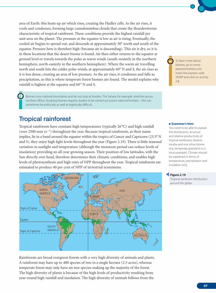
Tropical rainforestTropical rainforests have constant high temperatures (typically 26 °C) and high rainfall (over 2500 mm yr –1) throughout the year. Because tropical rainforests, as their name implies, lie in a band around the equator within the tropics of Cancer and Capricorn (23.5° N and S), they enjoy high light levels throughout the year (Figure 2.19). There is little seasonal variation in sunlight and temperature (although the monsoon period can reduce levels of insolation) providing an all-year growing season. Their position of low latitudes, with the Sun directly over head, therefore determines their climatic conditions, and enables high levels of photosynthesis and high rates of NPP throughout the year. Tropical rainforests are estimated to produce 40 per cent of NPP of terrestrial ecosystems.

Equator

Tropic of Cancer

Tropic of Capricorn

NORTH AMERICA

SOUTH AMERICA

AFRICA

GREENLAND

EUROPE

ASIA

AUSTRALIA

Rainforests are broad evergreen forests with a very high diversity of animals and plants. A rainforest may have up to 480 species of tree in a single hectare (2.5 acres), whereas temperate forest may only have six tree species making up the majority of the forest. The high diversity of plants is because of the high levels of productivity resulting from year-round high rainfall and insolation. The high diversity of animals follows from the

To learn more about biomes, go to www.pearsonhotlinks.com, insert the express code 2630P and click on activity 2.8.

Examiner’s hint:You need to be able to explain the distribution, structure and relative productivity of tropical rainforests, deserts, tundra and one other biome (e.g. temperate grassland or a local example). Climate should be explained in terms of temperature, precipitation and insolation only.

Figure 2.19Tropical rainforest distribution around the globe.

02_M02_14_82.indd 37 15/04/2010 08:56

38

THE ECOSYSTEM2

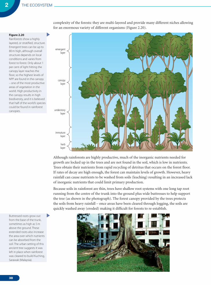
complexity of the forests: they are multi-layered and provide many different niches allowing for an enormous variety of different organisms (Figure 2.20).

emergentlayer

canopylayer

understorylayer

immaturelayer

herblayer

Although rainforests are highly productive, much of the inorganic nutrients needed for growth are locked up in the trees and are not found in the soil, which is low in nutrients. Trees obtain their nutrients from rapid recycling of detritus that occurs on the forest floor. If rates of decay are high enough, the forest can maintain levels of growth. However, heavy rainfall can cause nutrients to be washed from soils (leaching) resulting in an increased lack of inorganic nutrients that could limit primary production.

Because soils in rainforest are thin, trees have shallow root systems with one long tap root running from the centre of the trunk into the ground plus wide buttresses to help support the tree (as shown in the photograph). The forest canopy provided by the trees protects the soils from heavy rainfall – once areas have been cleared through logging, the soils are quickly washed away (eroded) making it difficult for forests to re-establish.

Figure 2.20Rainforests show a highly layered, or stratified, structure. Emergent trees can be up to 80 m high, although overall structure depends on local conditions and varies from forest to forest. Only about 1 per cent of light hitting the canopy layer reaches the floor, so the highest levels of NPP are found in the canopy – one of the most productive areas of vegetation in the world. High productivity in the canopy results in high biodiversity, and it is believed that half of the world’s species could be found in rainforest canopies.

Buttressed roots grow out from the base of the trunk, sometimes as high as 5 m above the ground. These extended roots also increase the area over which nutrients can be absorbed from the soil. The urban setting of this ancient tree suggests it was left in place when rainforest was cleared to build Kuching, Sarawak (Malaysia).

02_M02_14_82.indd 38 15/04/2010 08:56

39

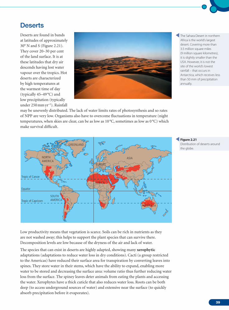
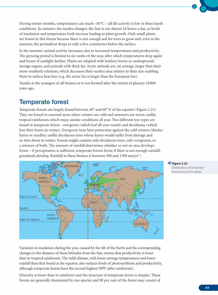
DesertsDeserts are found in bands at latitudes of approximately 30° N and S (Figure 2.21). They cover 20–30 per cent of the land surface. It is at these latitudes that dry air descends having lost water vapour over the tropics. Hot deserts are characterized by high temperatures at the warmest time of day (typically 45–49 °C) and low precipitation (typically under 250 mm yr–1). Rainfall may be unevenly distributed. The lack of water limits rates of photosynthesis and so rates of NPP are very low. Organisms also have to overcome fluctuations in temperature (night temperatures, when skies are clear, can be as low as 10 °C, sometimes as low as 0 °C) which make survival difficult.

Equator

Tropic of Cancer

Tropic of Capricorn

NORTHAMERICA

SOUTHAMERICA

AFRICA

GREENLAND

EUROPE

ASIA

AUSTRALIA

Low productivity means that vegetation is scarce. Soils can be rich in nutrients as they are not washed away; this helps to support the plant species that can survive there. Decomposition levels are low because of the dryness of the air and lack of water.

The species that can exist in deserts are highly adapted, showing many xerophytic adaptations (adaptations to reduce water loss in dry conditions). Cacti (a group restricted to the Americas) have reduced their surface area for transpiration by converting leaves into spines. They store water in their stems, which have the ability to expand, enabling more water to be stored and decreasing the surface area : volume ratio thus further reducing water loss from the surface. The spiney leaves deter animals from eating the plants and accessing the water. Xerophytes have a thick cuticle that also reduces water loss. Roots can be both deep (to access underground sources of water) and extensive near the surface (to quickly absorb precipitation before it evaporates).

The Sahara Desert in northern Africa is the world’s largest desert. Covering more than 3.5 million square miles (9 million square kilometres), it is slightly smaller than the USA. However, it is not the site of the world’s lowest rainfall – that occurs in Antarctica, which receives less than 50 mm of precipitation annually.

Figure 2.21Distribution of deserts around the globe.

02_M02_14_82.indd 39 15/04/2010 08:56

40

THE ECOSYSTEM2

Animals have also adapted to desert conditions. Snakes and reptiles are the commonest vertebrates – they are highly adapted to conserve water and their cold-blooded metabolism is ideally suited to desert conditions. Mammals have adapted to live underground and emerge at the coolest parts of day.

Tundra

Tundra is found at high latitudes, adjacent to ice margins, where insolation is low (Figure 2.22). Short day length also limits levels of sunlight. Water may be locked up in ice for months at a time and this combined with little rainfall means that water is also a limiting factor. Lack of light and rainfall mean that rates of photosynthesis and productivity are low. Temperatures are very low for most of the year; temperature is also a limiting factor because it affects the rate of photosynthesis, respiration and decomposition (these enzyme-driven chemical reactions are slower in colder conditions). Soil may be permanently frozen (permafrost) and nutrients are limiting. Low temperature means that the recycling of nutrients is low, leading to the formation of peat bogs where much carbon is stored. The vegetation consists of low scrubs and grasses.

Equator

Tropic of Cancer

Tropic of Capricorn

NORTHAMERICA

SOUTHAMERICA

AFRICA

GREENLAND

EUROPE

ASIA

AUSTRALIA

Most of the world’s tundra is found in the north polar region (Figure 2.22), and so is known as Arctic tundra. There is a small amount of tundra in parts of Antarctica that are not covered with ice, and on high altitude mountains (alpine tundra).

Elk crossing frozen tundra.

Figure 2.22Map showing the distribution of tundra around the globe.

02_M02_14_82.indd 40 15/04/2010 08:56

41

During winter months, temperatures can reach –50 °C – all life activity is low in these harsh conditions. In summer, the tundra changes: the Sun is out almost 24 hours a day, so levels of insolation and temperature both increase leading to plant growth. Only small plants are found in this biome because there is not enough soil for trees to grow and, even in the summer, the permafrost drops to only a few centimetres below the surface.

In the summer, animal activity increases, due to increased temperatures and productivity. The growing period is limited to six weeks of the year, after which temperatures drop again and hours of sunlight decline. Plants are adapted with leathery leaves or underground storage organs, and animals with thick fur. Arctic animals are, on average, larger than their more southerly relations, which decreases their surface area relative to their size enabling them to reduce heat loss (e.g. the arctic fox is larger than the European fox).

Tundra is the youngest of all biomes as it was formed after the retreat of glaciers 10 000 years ago.

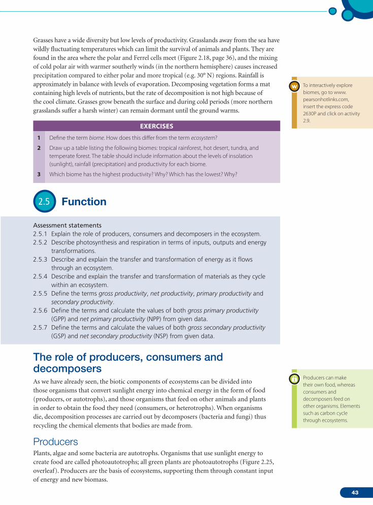
Temperate forestTemperate forests are largely found between 40° and 60° N of the equator (Figure 2.23). They are found in seasonal areas where winters are cold and summers are warm, unlike tropical rainforests which enjoy similar conditions all year. Two different tree types are found in temperate forest – evergreen (which leaf all year round) and deciduous (which lose their leaves in winter). Evergreen trees have protection against the cold winters (thicker leaves or needles) unlike deciduous trees whose leaves would suffer frost damage and so shut down in winter. Forests might contain only deciduous trees, only evergreens, or a mixture of both. The amount of rainfall determines whether or not an area develops forest – if precipitation is sufficient, temperate forests form; if there is not enough rainfall, grasslands develop. Rainfall in these biomes is between 500 and 1500 mm yr–1.

Equator

Tropic of Cancer

Tropic of Capricorn

NORTH AMERICA

SOUTH AMERICA

AFRICA

GREENLAND

EUROPE

ASIA

AUSTRALIA

Variation in insolation during the year, caused by the tilt of the Earth and the corresponding changes in the distance of these latitudes from the Sun, means that productivity is lower than in tropical rainforests. The mild climate, with lower average temperatures and lower rainfall than that found at the equator, also reduces levels of photosynthesis and productivity, although temperate forests have the second highest NPP (after rainforests).

Diversity is lower than in rainforest and the structure of temperate forest is simpler. These forests are generally dominated by one species and 90 per cent of the forest may consist of

Figure 2.23Distribution of temperate forest around the globe.

02_M02_14_82.indd 41 15/04/2010 08:56

42

THE ECOSYSTEM2

only six tree species. There is some layering of the forest, although the tallest trees generally do not grow more than 30 m, so vertical stratification is limited. The less complex structure of temperate forests compared to rainforest reduces the number of available niches and therefore species diversity is much less. The forest floor has a reasonably thick leaf layer that is rapidly broken down when temperatures are higher, and nutrient availability is in general not limiting. The lower and less dense canopy means that light levels on the forest floor are higher than in rainforest, so the shrub layer can contain many plants such as brambles, grasses, bracken and ferns.

Grassland

Grasslands are found on every continent except Antarctica, and cover about 16 per cent of the Earth’s surface (Figure 2.24). They develop where there is not enough precipitation to support forests, but enough to prevent deserts forming. There are several types of grassland: the Great Plains and the Russian Steppes are temperate grasslands; the savannas of east Africa are tropical grassland.

Equator

Tropic of Cancer

Tropic of Capricorn

NORTH AMERICA

SOUTH AMERICA

AFRICA

GREENLAND

EUROPE ASIA

AUSTRALIA

The loss of leaves from deciduous trees over winter allows increased insolation of the forest floor, enabling the seasonal appearance of species such as bluebells.

Bison roaming on mixed grass prairie.

Figure 2.24The distribution of grasslands around the globe.

Assessment statements2.5.1 Explain the role of producers, consumers and decomposers in the ecosystem.2.5.2 Describe photosynthesis and respiration in terms of inputs, outputs and energy

transformations.2.5.3 Describe and explain the transfer and transformation of energy as it flows

through an ecosystem.2.5.4 Describe and explain the transfer and transformation of materials as they cycle

within an ecosystem.2.5.5 Define the terms gross productivity, net productivity, primary productivity and

secondary productivity.2.5.6 Define the terms and calculate the values of both gross primary productivity

(GPP) and net primary productivity (NPP) from given data.2.5.7 Define the terms and calculate the values of both gross secondary productivity

(GSP) and net secondary productivity (NSP) from given data.

02_M02_14_82.indd 42 15/04/2010 08:56

43

Grasses have a wide diversity but low levels of productivity. Grasslands away from the sea have wildly fluctuating temperatures which can limit the survival of animals and plants. They are found in the area where the polar and Ferrel cells meet (Figure 2.18, page 36), and the mixing of cold polar air with warmer southerly winds (in the northern hemisphere) causes increased precipitation compared to either polar and more tropical (e.g. 30° N) regions. Rainfall is approximately in balance with levels of evaporation. Decomposing vegetation forms a mat containing high levels of nutrients, but the rate of decomposition is not high because of the cool climate. Grasses grow beneath the surface and during cold periods (more northern grasslands suffer a harsh winter) can remain dormant until the ground warms.

EXERCIsEs

1

2

3

Define the term biome. How does this differ from the term ecosystem?

Draw up a table listing the following biomes: tropical rainforest, hot desert, tundra, and temperate forest. The table should include information about the levels of insolation (sunlight), rainfall (precipitation) and productivity for each biome.

Which biome has the highest productivity? Why? Which has the lowest? Why?

2.5 Function

To interactively explore biomes, go to www.pearsonhotlinks.com, insert the express code 2630P and click on activity 2.9.

Assessment statements2.5.1 Explain the role of producers, consumers and decomposers in the ecosystem.2.5.2 Describe photosynthesis and respiration in terms of inputs, outputs and energy

transformations.2.5.3 Describe and explain the transfer and transformation of energy as it flows

through an ecosystem.2.5.4 Describe and explain the transfer and transformation of materials as they cycle

within an ecosystem.2.5.5 Define the terms gross productivity, net productivity, primary productivity and

secondary productivity.2.5.6 Define the terms and calculate the values of both gross primary productivity

(GPP) and net primary productivity (NPP) from given data.2.5.7 Define the terms and calculate the values of both gross secondary productivity

(GSP) and net secondary productivity (NSP) from given data.

The role of producers, consumers and decomposersAs we have already seen, the biotic components of ecosystems can be divided into those organisms that convert sunlight energy into chemical energy in the form of food (producers, or autotrophs), and those organisms that feed on other animals and plants in order to obtain the food they need (consumers, or heterotrophs). When organisms die, decomposition processes are carried out by decomposers (bacteria and fungi) thus recycling the chemical elements that bodies are made from.

ProducersPlants, algae and some bacteria are autotrophs. Organisms that use sunlight energy to create food are called photoautotrophs; all green plants are photoautotrophs (Figure 2.25, overleaf). Producers are the basis of ecosystems, supporting them through constant input of energy and new biomass.

Producers can make their own food, whereas consumers and decomposers feed on other organisms. Elements such as carbon cycle through ecosystems.

02_M02_14_82.indd 43 15/04/2010 08:56

44

THE ECOSYSTEM2

leaf surface

energy in sunlightenters chloroplastsin leaf cells

leaf underside

carbon dioxidein air enters leafthrough stomata

watertransportedinto leaffrom rootby xylem

sugarstransportedaway fromleaf byphloem

ConsumersConsumers do not contain photosynthetic pigments such as chlorophyll so they cannot make their own food. They must obtain their energy, minerals and nutrients by eating other organisms – they are heterotrophs. Herbivores feed on autotrophs, carnivores feed on other heterotrophs, and omnivores feed on both. Whereas autotrophs convert inorganic compounds into organic ones, heterotrophs do the opposite.

DecomposersDecomposers obtain their food and nutrients from the breakdown of dead organic matter. When they break down tissue, they release nutrients ready for reabsorption by producers. They form the basis of a decomposer food chain (which may be energetically more important in some ecosystems than grazing food chains). Decomposers also contribute to the build up of humus and improve nutrient retention capacity in soil through incomplete breakdown of organic material.

Some bacteria found in the soil are autotrophs, but rather than use sunlight to obtain the energy to create complex organic molecules, they use chemical energy from oxidation reactions. These bacteria are called chemoautotrophs – they are key players in the nitrogen cycle (page 49). They convert ammonia from decomposing organisms and excretory waste into nitrites and then nitrates. Plants can take in nitrates through their root systems. Chemoautotrophs can therefore form the basis of food chains.

Photosynthesis and respirationTwo processes control the flow of energy through ecosystems: photosynthesis and respiration. Photosynthesis stores energy in biomass and respiration releases this energy so that it can be used to support the organisms’ life processes.

Figure 2.25Plants absorb carbon dioxide from air and water from soil. Sunlight enters through the upper epidermis and strikes chlorophyll in chloroplasts of leaf cells. In the chloroplasts, the energy in sunlight is used to combine the water and carbon dioxide into glucose – a store of chemical energy.

02_M02_14_82.indd 44 15/04/2010 08:56

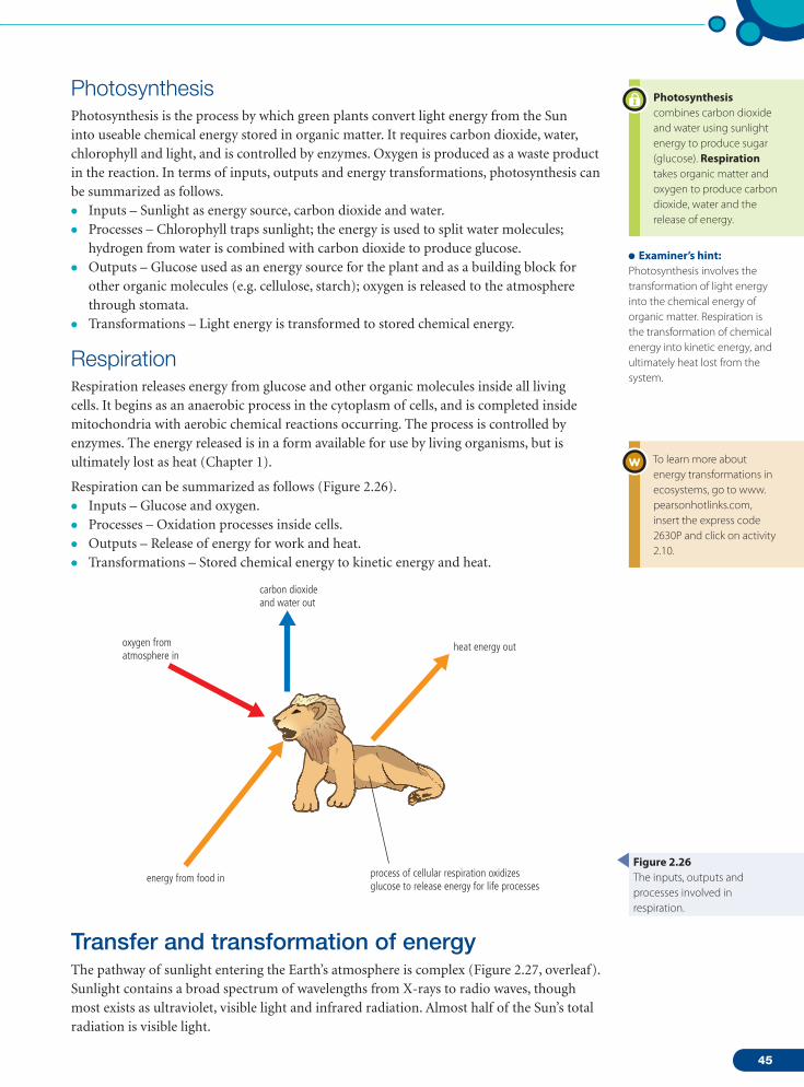
45

PhotosynthesisPhotosynthesis is the process by which green plants convert light energy from the Sun into useable chemical energy stored in organic matter. It requires carbon dioxide, water, chlorophyll and light, and is controlled by enzymes. Oxygen is produced as a waste product in the reaction. In terms of inputs, outputs and energy transformations, photosynthesis can be summarized as follows.• Inputs – Sunlight as energy source, carbon dioxide and water.• Processes – Chlorophyll traps sunlight; the energy is used to split water molecules;

hydrogen from water is combined with carbon dioxide to produce glucose.• Outputs – Glucose used as an energy source for the plant and as a building block for

other organic molecules (e.g. cellulose, starch); oxygen is released to the atmosphere through stomata.

• Transformations – Light energy is transformed to stored chemical energy.

RespirationRespiration releases energy from glucose and other organic molecules inside all living cells. It begins as an anaerobic process in the cytoplasm of cells, and is completed inside mitochondria with aerobic chemical reactions occurring. The process is controlled by enzymes. The energy released is in a form available for use by living organisms, but is ultimately lost as heat (Chapter 1).

Respiration can be summarized as follows (Figure 2.26).• Inputs – Glucose and oxygen.• Processes – Oxidation processes inside cells.• Outputs – Release of energy for work and heat.• Transformations – Stored chemical energy to kinetic energy and heat.

energy from food in process of cellular respiration oxidizesglucose to release energy for life processes

oxygen from atmosphere in

heat energy out

carbon dioxide and water out

Transfer and transformation of energyThe pathway of sunlight entering the Earth’s atmosphere is complex (Figure 2.27, overleaf). Sunlight contains a broad spectrum of wavelengths from X-rays to radio waves, though most exists as ultraviolet, visible light and infrared radiation. Almost half of the Sun’s total radiation is visible light.

Figure 2.26The inputs, outputs and processes involved in respiration.

Examiner’s hint:Photosynthesis involves the transformation of light energy into the chemical energy of organic matter. Respiration is the transformation of chemical energy into kinetic energy, and ultimately heat lost from the system.

photosynthesis combines carbon dioxide and water using sunlight energy to produce sugar (glucose). Respiration takes organic matter and oxygen to produce carbon dioxide, water and the release of energy.

To learn more about energy transformations in ecosystems, go to www.pearsonhotlinks.com, insert the express code 2630P and click on activity 2.10.

02_M02_14_82.indd 45 15/04/2010 08:56

46

THE ECOSYSTEM2

reflectedsolar energy

107solar energy

342

infrared energy

235

reflected by clouds, aerosol and atmospheric

gases 77

absorbed byatmosphere

67

thermals24

40

40

emitted byatmosphere 165 greenhouse

gasesemitted byclouds 30

latentheat 78

350 235back

radiation

235absorbed by surface

168 absorbed by surface

390 surface radiation evapotranspiration

78

reflected by surface

30

Very little of the sunlight available from the Sun ends up as biomass in ecosystems. First, much of the incoming solar radiation fails to enter the chloroplasts of leaves because it is reflected, transmitted or is the wrong wavelength to be absorbed (Figure 2.1, page 15). Of the radiation captured by leaves, only a small percentage ends up as biomass in growth compounds the conversion of light to chemical energy is inefficient. Overall, only around 0.06 per cent of all the solar radiation falling on the Earth is captured by plants.

Once converted into a chemical store, energy is available in useable form both to the producers and to organisms higher up the food chain. As we saw in Chapter 1, there is loss of chemical energy from one trophic level to another. The percentage of energy transferred from one trophic level to the next is called the ecological efficiency: these efficiencies of transfer are low and they account for the energy loss. Ecological efficiency varies between 5 and 20 per cent with an average of 10 per cent: on average, one tenth of the energy available to one trophic level becomes available to the next.

Ultimately all energy lost from an ecosystem is in the form of heat, through the inefficient energy conversions of respiration, so overall there is a conversion of light energy to heat energy by an ecosystem. Heat energy is re-radiated into the atmosphere.

Energy stores and flowsWe have seen how diagrams can be used to show energy flow through ecosystems. Stores of energy are usually shown as boxes (other shapes may be used) which represent the various trophic levels. Flows of energy are usually shown as arrows (with the amount of energy in joules or biomass per unit area). Arrows can also show productivity (rates in J m–2 day–1). Varying width of the arrows indicates proportionally how much energy or productivity is flowing at any point in the diagram.

Energy flow can be shown in the form of Sankey diagrams (Figure 2.28). The relative width of the bands (which can also be shown as arrows) represents the relative amount of energy flowing in joules. In Figure 2.28, mammals lose more energy to the environment as a result of the high levels of respiration needed to maintain body temperature and higher activity. Herbivores eat only plants so they take in contain large amounts of indigestible substances such as cellulose (in plant cell walls); the energy in indigestible substances is not absorbed, so is lost in faeces.

Figure 2.27The Earth’s energy budget. Mean vertical energy flows in the terrestrial system (atmosphere and surface), in watts per square metre. Most important are the 342 W m–2 of solar energy which enter the outer atmospheric layer and the approximately 390 W m–2 which emanate from the soil in the form of infrared waves.

To learn more about energy stores and flows in an ecosystem, go to www.pearsonhotlinks.com, insert the express code 2630P and click on activity 2.11.

Not all solar radiation ends up being stored as biomass. Losses include:• reflection from leaves• light not hitting

chloroplasts• light of the wrong

wavelengths (not absorbed by chloroplast pigments)

• transmission of light through the leaf

• inefficiency of photosynthesis.

02_M02_14_82.indd 46 15/04/2010 08:56

47

Invertebrate herbivore Invertebrate carnivore Mammal herbivore Mammal carnivore

I = IntakeR = RespirationA = Absorbed from

foodF = Lost in faecesP = Passed on to

next trophic level

R

P

A

FI

R

P

A

F

I

R

P

A

FI

R

P

AF

I

R

P

A

FI

R

P

A

F

I

R

P

A

FI

R

P

AF

I

R

P

A

FI

R

P

A

F

I

R

P

A

FI

R

P

AF

I

R

P

A

FI

R

P

A

F

I

R

P

A

FI

R

P

AF

I

Productivity diagrams were pioneered by American scientist Howard Odum in the 1950s. He carried out the first complete analysis of a natural ecosystem (a spring-fed stream) at Silver Spring in Florida. He mapped in detail all the flow routes to and from the stream, and measured the energy and organic matter inputs and outputs, and from these calculated productivity for each trophic level and the flows between them. Productivity was calculated in kcal m–2 yr–1. From these figures he was able to draw the stream’s energy budget (Figure 2.29). The main inputs are sunlight and other biomass, and energy leaves the system as heat from respiration in animals and as decomposed matter (not shown in the diagram). He also drew the diagram in the form of a river system which showed the same information but in a more naturalized way. The information from the Silver Spring study can be simplified still further (Figure 2.30). Productivity diagrams such as these are more useful than simple energy flow diagrams as they give an indication of turnover in ecosystems by measuring energy flows per unit time as well as area.

primaryproducers

herbivore carnivore

LA = light absorbedPG = gross photosynthesis (GPP)PN = Net photosynthesis (PG – R) (NPP)R = respirationI = energy intakeNU = energy not used at the levelNA = energy ingested but not assimilatedA = energy assimilated

Adapted from Food and AgricultureOrganization of the United Nations

source:

PG

PN

LA

R

R

A I

NU NU

NA

NA

R R

sunlight

heat heat

top carnivore

energy lost as heat

photosynthesis H C

D

cellular respiration heat

TC

solar energy

imported nutrients and organic matter

H = herbivores C = carnivores TC = top carnivores D = decomposers

Figure 2.28Energy flow in animals. Diagrams show energy flow through four types of animals. The diagrams are drawn to scale so that the width of the sections enables comparisons to be made.

Figure 2.29Productivity in a stream ecosystem at Silver Spring, Florida. Boxes show levels of productivity at each trophic level, from producers through to top carnivores, and linking bands (or arrows) show the flow of energy. (NPP and GPP are discussed later in this chapter.) Decomposers are not included in the diagram. Size relations in the diagram are approximate but not precisely to scale. Units are kcal m–2 yr–1 (1 kcal = 4.2 J).

Figure 2.30Energy flows through an ecosystem simplified from Odum’s Silver Springs model. Squares represent stores of biomass and ovals are movements of energy from the system. Arrows are approximately proportional to each other and indicate differences in energy flow between different parts of the system.

To learn more about Howard Odum and his work, go to www.pearsonhotlinks.com, insert the express code 2630P and click on activity 2.12.

02_M02_14_82.indd 47 15/04/2010 08:56

48

THE ECOSYSTEM2

Transfer and transformation of materials within an ecosystemCarbon cycleUnlike energy, nutrients can be recycled and reused in ecosystems. Without this recycling, the Earth would be covered with detritus and the availability of nutrients would decline. Decomposition is at the centre of these nutrient cycles, but other processes play their part as well.

Carbon is an essential element in ecosystems as it forms the key component of biological molecules (e.g. carbohydrates, fats and protein). Although ecosystems form an important store of carbon (especially trees), it is also stored in fossil fuels (coal, gas, peat and oil) and in limestone, and can remain in these forms for very long periods of time (Figure 2.31).

carbon dioxide (CO2) in air

CO2 dissolves in water;carbon fixed byphotosynthesisinto biomass of algaeand phytoplankton

carbon fixed by photosynthesis into green plant biomass

cell respiration by aquatic and terrestrial plants, animals and decomposers

sedimentation of biomass conversion to coal,

oil, natural gas (fossil fuels)

combustion of fossil fuels

weathering volcanism

carbon fixed into calcium carbonate of shells (limestone)

fires

feeding by heterotrophs

plant respiration

millions of years

millions of years

shellfish

solarenergy

Carbon dioxide is fixed (i.e. converted from a simple inorganic molecule into a complex organic molecule – glucose) by autotrophs in either aquatic or terrestrial systems. These organisms respire and return some carbon into the atmosphere as carbon dioxide, or assimilate it into their bodies as biomass. When the organisms die, they are consumed by decomposers which use the dead tissue as a source of food, returning carbon to the atmosphere when they respire.

Oil and gas were formed millions of years ago when marine organisms died and fell to the bottom of the ocean, where anaerobic conditions halted the decay process. Burial of the organisms followed by pressure and heat over long periods of time created these fuels. Coal was formed largely by similar processes acting on land vegetation. Limestone (calcium carbonate) was formed by the shells of ancient organisms and corals being crushed and compressed into sedimentary rock. Weathering of limestone, acid rain, and the burning of fossil fuels, returns carbon to the atmosphere.

Figure 2.31Carbon stores and movement between them.

02_M02_14_82.indd 48 15/04/2010 08:56

49

Nitrogen cycleNitrogen is an essential building block of amino acids (which link together to make proteins) and nucleic acids (which form the basis of DNA). It is a vital element for all organisms.

Nitrogen is the most abundant gas in the atmosphere (80 per cent) but because it is very stable (the two nitrogen atoms in a nitrogen molecule are triple-bonded) it is not directly accessible by animals or plants. Only certain species of bacteria (nitrogen-fixing bacteria) can generate the energy needed to split the triple bond to convert nitrogen gas into ammonia.

The nitrogen cycle (Figure 2.32) is driven by four types of bacteria:• nitrogen-fixing bacteria• decomposers• nitrifying bacteria• denitrifying bacteria.

nitrogen in atmosphere

plant and microbial protein

absorbed by plant roots feeding

nitrates

nitrites

animal protein

death

dead organic matter and faeces

ammonia, ammonium compounds decay by saprotrophic

bacteria and fungi

denitrifying bacteria

death and defecation

free-living nitrogen-fixing bacteria (e.g. Azotobacter)

symbiotic nitrogen-fixing bacteria (Rhizobium)

nitrifying bacteria

nitrifying bacteria

lightning

Haber process

Nitrogen-fixing bacteria are found either free-living in the soil (e.g. Azotobacter) or living within root nodules of leguminous plants (Rhizobium). Species in root nodules are symbiotic with the plant – they derive the sugars they need for respiration from the plant (a lot of energy is needed to split the nitrogen molecule) and the plants gain a useable form of nitrogen.

Lightning can fix atmospheric nitrogen into ammonia. Decomposers produce ammonia and ammonium compounds. Ammonia is also present in excretory products.

Nitrifying bacteria found in the soil oxidize the ammonia first into nitrites and then into nitrates. The bacteria gain energy from this reaction to form food (they are chemoautotrophs). Ammonia and nitrites are toxic to plants but the nitrates are taken up with water into plant roots and used to create amino acids and other organic chemicals.

Nitrogen is returned to the atmosphere by denitrifying bacteria, which remove oxygen from nitrates for use in respiration (they live in oxygen-poor soils where free oxygen is not

Figure 2.32Flows and storage of nitrogen in ecosystems.

02_M02_14_82.indd 49 15/04/2010 08:56

50

THE ECOSYSTEM2

readily available). Nitrogen gas is released as a by-product. The reason that water-logged soils are not good for farmers is that denitrifying bacteria enjoy these conditions and dramatically reduce the quantity of nitrates available for crop growth.

The breakdown of organic matter is higher in tropical forest than in temperate woodland because high temperatures and year-round availability of water in tropical forests allow for continuous breakdown of nitrogen-containing compounds. This results in very rapid turn-around and reabsorption. In temperate woodland, the breakdown of organic matter slows down significantly during winter months, causing nitrogen build up in soil.

Some tropical forest trees have specific species of mycorrhizal fungi associated with their roots that increase rate of organic matter breakdown leading to rapid reabsorption of nitrogen. Although soils are nutrient poor in tropical forests, the rapid recycling of nitrogen compared to temperate forests therefore allows for more rapid growth to occur.

Nutrient cyclesNutrient cycles can be shown in simple diagrams which show stores and transfers of nutrients (Figure 2.33).

input dissolved in rainfall

uptake by plants

decay

degradation andmineralizationloss in

run-off

loss through leaching input weathered

from rock

litter

biomass

soil

The factors that affect the store of nutrients and their transfer are those that affect: • the amount and type of weathering• overland run-off and soil erosion• eluviations• the amount of rainfall• rates of decomposition• the nature of vegetation (woody species hold onto nutrients for much longer than

annuals)• the age and health of plants• plant density• fire.

Hence, explaining the differences between nutrient cycles in different ecosystems involves a consideration of many processes.

Mycorrhizae attached to plant roots, form a thread-like network, extending beyond the roots. This extra network takes up additional water and nutrients and supplies them to the plant.

Figure 2.33Gersmehl’s nutrient cycle.

02_M02_14_82.indd 50 15/04/2010 08:56

51

Nutrients are circulated and re-used frequently. All natural elements are capable of being absorbed by plants, either as gases or as soluble salts. Only oxygen, carbon, hydrogen and nitrogen are needed in large quantities. These are known as macronutrients. The rest are trace elements or micronutrients and are needed only in small quantities (e.g. magnesium, sulfur and phosphorus). Nutrients are taken in by plants and built into new organic matter. When animals eat the plants, they take up the nutrients. The nutrients eventually return to the soil when the plants and animals die and are broken down by the decomposers.

All nutrient cycles involve interaction between soil and the atmosphere, and many food chains. Nevertheless, there is great variety between the cycles. Nutrient cycles can be sedimentary based, in which the source of the nutrient is from rocks, or they can be atmospheric based, as in the case of the nitrogen cycle. Generally, gaseous cycles are more complete than sedimentary ones, as the latter are more easily disturbed, especially by human activity.

Global water cycleThe hydrological cycle refers to the cycle of water between atmosphere, lithosphere and biosphere (Figure 2.34).

ocean (1 348 million km3)

groundwater (8.0 million km3)

run-off from land (40 000 km3)

lakes and rivers (200 000 km3)

snow and ice (29 million km3)

evaporation from land (70 000 km3)

precipitation over land (110 000 km3)

water vapour in atmosphere (13 000 km3)

precipitation over ocean (390 000 km3)

evaporation from ocean (430 000 km3)

Figure 2.34The global water cycle.

02_M02_14_82.indd 51 15/04/2010 08:56

52

THE ECOSYSTEM2

At a local scale, the cycle has a single input (precipitation, PPT) and two major outputs (evapotranspiration, EVT, and run-off). A third output (leakage) may also occur from the deeper subsurface to other basins.

Throughput refers to the transfer of water through the system. Water can be stored at a number of stages or levels within the cycle. These stores include vegetation, surface, soil moisture, groundwater and water channels. The global hydrological cycle also includes the oceans and the atmosphere.

Human modifications are made at every scale. Good examples include large scale changes of channel flow and storage, irrigation and land drainage, and large-scale abstraction of groundwater and surface water for domestic and industrial use.

To learn more about the water, carbon and nitrogen cycles, using a systems approach, go to www.pearsonhotlinks.com, insert the express code 2630P and click on activity 2.13.

EXERCIsEs

1

2

3

4

5

Explain the role of producers, consumers and decomposers in the ecosystem.

Summarize photosynthesis in terms of inputs, outputs and energy transformations. Now do the same for respiration.

(a) Why is not all available light energy transformed into chemical energy in biomass? (b) Why is not all of the energy in biomass made available to the next tropic level?

Construct a simple energy-flow diagram illustrating the movement of energy through ecosystems, including the productivity of the various trophic levels.

Draw systems diagrams for each of the following cycles:• the carbon cycle• the nitrogen cycle• the water cycle.

Each should contain storages, flows, transfers and transformations.

Definitions: gross primary productivity, net primary productivity, and secondary productivityWe have already looked at productivity in ecosystems and described it as production per unit time. Productivity can be divided into primary and secondary productivity defined as follows.• Primary productivity – The gain by producers (autotrophs) in energy or biomass

per unit area per unit time.• Secondary productivity – The biomass gained by heterotrophic organisms, through

feeding and absorption, measured in units of mass or energy per unit area per unit time.

Primary productivity is the conversion of solar energy whereas secondary productivity involves feeding or absorption. Primary productivity depends on the amount of sunlight, the ability of producers to use energy to synthesize organic compounds, and the availability of other factors needed for growth (e.g. minerals and nutrients) (Figure 2.35).

Secondary productivity depends on the amount of food present and the efficiency of consumers turning this into new biomass.

Productivity is production per unit time.

02_M02_14_82.indd 52 15/04/2010 08:56

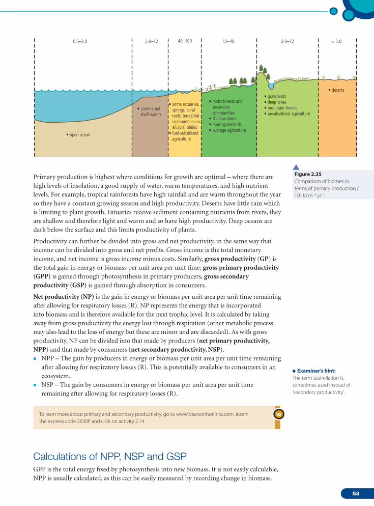
53

< 2.0

• deserts• grasslands• deep lakes• mountain forests• unsubsidized agriculture

• moist forests and secondary communities• shallow lakes• moist grasslands• average agriculture

• some estuaries, springs, coral reefs, terrestrial communities on alluivial plains• fuel-subsidized agriculture

• continental shelf waters

• open ocean

0.5–3.0 2.0–12 40–100 12–40 2.0–12

Primary production is highest where conditions for growth are optimal – where there are high levels of insolation, a good supply of water, warm temperatures, and high nutrient levels. For example, tropical rainforests have high rainfall and are warm throughout the year so they have a constant growing season and high productivity. Deserts have little rain which is limiting to plant growth. Estuaries receive sediment containing nutrients from rivers, they are shallow and therefore light and warm and so have high productivity. Deep oceans are dark below the surface and this limits productivity of plants.

Productivity can further be divided into gross and net productivity, in the same way that income can be divided into gross and net profits. Gross income is the total monetary income, and net income is gross income minus costs. Similarly, gross productivity (GP) is the total gain in energy or biomass per unit area per unit time; gross primary productivity (GPP) is gained through photosynthesis in primary producers, gross secondary productivity (GSP) is gained through absorption in consumers.

Net productivity (NP) is the gain in energy or biomass per unit area per unit time remaining after allowing for respiratory losses (R). NP represents the energy that is incorporated into biomass and is therefore available for the next trophic level. It is calculated by taking away from gross productivity the energy lost through respiration (other metabolic process may also lead to the loss of energy but these are minor and are discarded). As with gross productivity, NP can be divided into that made by producers (net primary productivity, NPP) and that made by consumers (net secondary productivity, NSP).• NPP – The gain by producers in energy or biomass per unit area per unit time remaining

after allowing for respiratory losses (R). This is potentially available to consumers in an ecosystem.

• NSP – The gain by consumers in energy or biomass per unit area per unit time remaining after allowing for respiratory losses (R).

Calculations of NPP, NSP and GSP GPP is the total energy fixed by photosynthesis into new biomass. It is not easily calculable, NPP is usually calculated, as this can be easily measured by recording change in biomass.

Figure 2.35Comparison of biomes in terms of primary production / 103 kJ m–2 yr–1.

Examiner’s hint:The term ‘assimilation’ is sometimes used instead of ‘secondary productivity’.

To learn more about primary and secondary productivity, go to www.pearsonhotlinks.com, insert the express code 2630P and click on activity 2.14.

02_M02_14_82.indd 53 15/04/2010 08:56

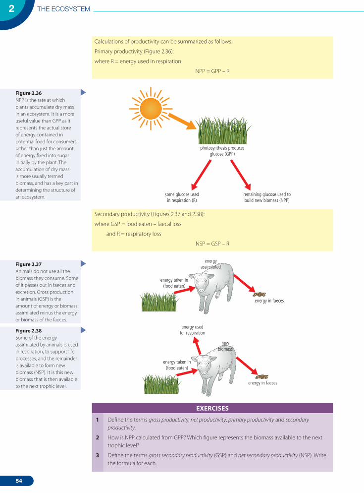
54

THE ECOSYSTEM2

Calculations of productivity can be summarized as follows:

Primary productivity (Figure 2.36):

where R = energy used in respiration

NPP = GPP – R

photosynthesis producesglucose (GPP)

remaining glucose used tobuild new biomass (NPP)

some glucose usedin respiration (R)

Secondary productivity (Figures 2.37 and 2.38):

where GSP = food eaten – faecal loss

and R = respiratory loss

NSP = GSP – R

energy taken in(food eaten)

energyassimilated

energy in faeces

energy taken in(food eaten)

energy usedfor respiration

newbiomass

energy in faeces

EXERCIsEs

1

2

3

Define the terms gross productivity, net productivity, primary productivity and secondary productivity.

How is NPP calculated from GPP? Which figure represents the biomass available to the next trophic level?

Define the terms gross secondary productivity (GSP) and net secondary productivity (NSP). Write the formula for each.

Figure 2.36NPP is the rate at which plants accumulate dry mass in an ecosystem. It is a more useful value than GPP as it represents the actual store of energy contained in potential food for consumers rather than just the amount of energy fixed into sugar initially by the plant. The accumulation of dry mass is more usually termed biomass, and has a key part in determining the structure of an ecosystem.

Figure 2.37Animals do not use all the biomass they consume. Some of it passes out in faeces and excretion. Gross production in animals (GSP) is the amount of energy or biomass assimilated minus the energy or biomass of the faeces.

Figure 2.38Some of the energy assimilated by animals is used in respiration, to support life processes, and the remainder is available to form new biomass (NSP). It is this new biomass that is then available to the next trophic level.

Assessment statements2.6.1 Explain the concepts of limiting factors and carrying capacity in the context of

population growth.2.6.2 Describe and explain S- and J- population curves.2.6.3 Describe the role of density-dependent and density-independent factors, and

internal and external factors, in the regulation of populations.2.6.4 Describe the principles associated with survivorship curves including, K- and

r-strategists.2.6.5 Describe the concept and processes of succession in a named habitat.2.6.6 Explain the changes in energy flow, gross and net productivity, diversity and

mineral cycling in different stages of succession.2.6.7 Describe factors affecting the nature of climax communities.

02_M02_14_82.indd 54 15/04/2010 08:56

55

4 NPP, mean biomass, and NPP per kg biomass vary in different biomes, depending on levels of insolation, rainfall and temperature. Mean NPP for tropical rainforest is greater than tundra because rainforest is hot and wet, so there is more opportunity to develop large biomass than in tundra. However, NPP per kg biomass is far lower in rainforest than tundra because rainforest has a high rate of both photosynthesis and respiration, so NPP compared to total biomass is low. Tundra are cold and dry and have low rates of photosynthesis and respiration; plants are slow growing with a gradual accumulation of biomass but relatively large growth in biomass per year.

The table below shows values for these parameters for different biomes.

Biome Mean net primary productivity (NPP) / kg m–2 yr–1

Mean biomass / kg m–2

NPP per kg biomass per year

desert 0.09 0.02

tundra 0.14 0.60 0.233

temperate grassland 0.60 1.60 0.375

savannah (tropical) grassland 0.90 4.00 0.225

temperate forest 1.20 32.50 0.037

tropical rainforest 2.20 45.00 0.049

(a) Calculate the NPP per kg of biomass per year for the desert biome.

(b) How does this figure compare those for other biomes? Explain the figure you have calculated in terms of NPP, and NPP per kg biomass.

(c) Compare the figures for NPP in temperate and tropical grassland. Explain the difference.

2.6 Changes

Assessment statements2.6.1 Explain the concepts of limiting factors and carrying capacity in the context of

population growth.2.6.2 Describe and explain S- and J- population curves.2.6.3 Describe the role of density-dependent and density-independent factors, and

internal and external factors, in the regulation of populations.2.6.4 Describe the principles associated with survivorship curves including, K- and

r-strategists.2.6.5 Describe the concept and processes of succession in a named habitat.2.6.6 Explain the changes in energy flow, gross and net productivity, diversity and

mineral cycling in different stages of succession.2.6.7 Describe factors affecting the nature of climax communities.

Limiting factors and carrying capacityPopulations are constrained by limiting factors. Carrying capacity is the maximum number of organisms that an area or ecosystem can sustainably support over a long period of time.

Limiting factors include temperature, water and nutrient availability. The main limiting climatic features are temperature and water availability. Every species has a tolerance range for any environmental factor; those with a wide range are described as stenoecious species, those with a narrow range are described as euryoecious species.

The concept of tolerance suggests that there are upper and lower levels of environmental factors beyond which a population cannot survive, and that there is an optimum range within which species can thrive (Figure 2.39, overleaf).

02_M02_14_82.indd 55 15/04/2010 08:56

56

THE ECOSYSTEM2

popu

latio

n

environmental gradient

optimal rangerange of

physiologicalstress

organismsinfrequent

range ofphysiological

stress

organismsinfrequent

range ofintolerance

organismsabsent

range ofintolerance

organismsabsent

tolerance range

high

lowlow high

Species at the lower end of the tolerance curve are known as oligotypic, those at the higher end are known as polytypic, and those in the middle are known as mesotypic.

Limiting factors are the factors that limit the distribution or numbers of a particular population. Limiting factors are environmental factors which slow down population growth.

Carrying capacity refers to the number of organisms – or size of population – that an area or ecosystem can support sustainably over a long period of time.

The term limiting factor was first used by the German agricultural chemist Justus von Liebig (1803–1873) who noted that the growth of crops was limited by the shortage of certain minerals. Liebig established the ‘law of minimum’ – that the productivity, reproduction and growth of organisms will be limited if one or more environmental factors lies below its limiting level. Equally, there can be too much of a factor (e.g. there is an upper limit to how much of a particular nutrient plants can tolerate).

TemperatureMany aspects of temperature affect species. These include daily, monthly and annual extremes, and mean temperatures. Temperature may be limiting at different stages in the life cycle – for example, some seeds in savannah grasslands will germinate only after high temperatures caused by fires. These fires enrich the soil with nutrients and kill off competitors thereby helping the survival chances of the seeds.

In most animals, temperature is a vital limiting factor. Cold-blooded animals can take advantage of sunny areas or warm rocks to heat their bodies. In hot deserts, animals are limited by excessive heat. To cope, some animals avoid the heat by burrowing, while others have physiological adaptations to tolerate high body temperatures.

Plants vary enormously in their ability to tolerate extremes of temperature. Categories of cold-tolerance in plants include the following.• Chill-sensitive – Plants are damaged below 10 °C (e.g. tropical plants).• Frost-sensitive – Plants can survive below 10 °C but are damaged if ice forms in their

tissues.• Frost-resistant – Plants can survive temperatures as low as –15 °C.• Frost-tolerant – Plants survive by withdrawing water from their cells, so preventing ice

from forming.• Cold-tolerant – Plants with needle-shaped leaves which can survive low temperatures.

WaterAll plants and animals need water to survive. For plants, water stress (i.e. too little water) may cause germination to fail, seedlings to die, and seed yield to be reduced. Water and temperature conditions vary around the world (Figure 2.40).

Figure 2.39The concept of tolerance.

02_M02_14_82.indd 56 15/04/2010 08:56

57

Mean annual totals

P = precipitationEt = potential evapotranspiration

precipitation soil moistureutilization

evaporation soil moisturedeficit

soil watersurplus

soil waterrecharge

temperature curve

0

25

50

75

100

125

150 mm

D A O J F M A M J J S N

0

30 °C

20

10

6°

Madrid

P = 436 mm Et = 759 mm

6°

London

P = 594 mm Et = 680 mm

0

25

50

75

100

125

150

0

20 °C

10

mm

D A O J F M A M J J S N

Mean annual totals

P = precipitationEt = potential evapotranspiration

precipitation soil moistureutilization

evaporation soil moisturedeficit

soil watersurplus

soil waterrecharge

temperature curve

0

25

50

75

100

125

150 mm

D A O J F M A M J J S N

0

30 °C

20

10

6°

Madrid

P = 436 mm Et = 759 mm

6°

London

P = 594 mm Et = 680 mm

0

25

50

75

100

125

150

0

20 °C

10

mm

D A O J F M A M J J S N

Plants are extremely sensitive to water level and categories of water-tolerant plants include the following.• Hydrophytes – Water-tolerant plants which can root in standing water.• Mesophytes – Plants that inhabit moist but not wet environments.• Xerophytes – Plants that live in dry environments.

Xerophyte adaptations to avoid water shortages include remaining as seeds until rain prompts germination, and storing water in stems, leaves or roots. Plants that store water are called succulents. Many succulents have a crassulacean acid metabolism (CAM) which allows them to take in carbon dioxide at night when their stomata are open, and use it during the day when the stomata are closed. Other xerophytes have thick, waxy cuticles, sunken and smaller stomata, and drop their leaves in dry periods.

S- and J-curvesThe S-curve has been recorded for the re-establishment of vegetation after the eruption of Krakatau in 1883 (Chapter 4, page 184) and the Mt St Helens eruption in 1980. The typical S-curve shows three stages:• exponential growth stage – in which the population grows at an increasingly rapid rate• transitional phase – where the population growth slows considerably – but it continues

to grow• plateau (or stationary) phase – in which the number of individuals stabilizes and

population growth stabilizes.

Exponential growth phaseIn this phase, if there are no limiting factors, a population can double in size on a regular basis. A population of rabbits, for example, can double every four months. A good example

Figure 2.40Climographs and soil moisture status.

Sigmoidal curves (s-curves) are population growth curves which show an initial rapid growth (exponential growth) and then slow down as the carrying capacity is reached. In some cases, there may be an overshoot, followed by die back (Figure 2.41a). In contrast, a J-curve is a population growth curve which shows only exponential growth. Growth is initially slow and becomes increasingly rapid; it does not slow down (Figure 2.41b).

popu

latio

n

time

popu

latio

n

time

(a)

(b)

Figure 2.41(a) S-curve.(b) J-curve.

02_M02_14_82.indd 57 15/04/2010 08:56

58

THE ECOSYSTEM2

of exponential growth is that of cane toads in Australia. The reasons for the exponential growth include:• plentiful resources such as light, space and food• lack of competition from other species• favourable abiotic factors such as temperature and rainfall• lack of predators or disease.

Transitional phaseIn this phase, unlimited growth declines as the factors listed above begin to change. The causes of the slowdown include:• increase in competition for resources because there are too many individuals in the

population• increase in predators attracted by the large population (food supply)• increase in rate of disease (and mortality) due to increased numbers of individuals living

in a small area.

Plateau phaseOver time, as available space and resources decrease, birth rates decline. As the risk of disease increases, mortality rates rise. This slows population growth. The combination of fewer births and increased mortality reinforce the decline in population increase. The population plateaus.

There is a limit to the size of a population that can be supported by an environment. Exponential increase can only occur when the population size is small in relation to the carrying capacity. Once the population exceeds the carrying capacity, death rates increase and population crashes may occur.

Long- and short-lived speciesSome populations have a cyclical explosion–crash cycle (Figure 2.42). Such a pattern characterizes fast-reproducing, short-lived species at lower trophic levels; examples include rodents, insects and annual plants. The numbers of these species are generally regulated by external factors such as climatic conditions, predators or nutrition (food supply).

popu

latio

n siz

e

time

overshoot

dieback

carrying capacity ofthe environment

Longer-lived species with few predators tend to follow the S-curve. Exponential growth is followed by slower growth due to density-dependent and density-independent factors. The population adapts to the environmental carrying capacity (Figure 2.43).

Figure 2.42Periodic population explosion and crash.

02_M02_14_82.indd 58 15/04/2010 08:56

59

popu

latio

n siz

e

time

S curve

carrying capacity ofthe environment

EXERCIsEs

1

2

The data below show rates of growth in ticklegrass (as above ground biomass in g m–2) in soils with low or high nitrogen content and using high or low seed density.

Year Low nitrogen, high seed density: above

ground biomass / g m–2

Low nitrogen, low seed density: above

ground biomass / g m–2

High nitrogen, high seed density: above

ground biomass / g m–2

High nitrogen, low seed density: above

ground biomass / g m–2

(a) Plot the data showing the growth rates among ticklegrass depending on nitrogen availability and density of seeds.

(b) Describe the results you have produced.

(c) Suggest reasons for these results.

1 0 0 0 0

2 420 60 500 30

3 780 80 1050 100

4 0 70 0 90

5 50 100 160 80

6 180 110 600 70

The table below shows population growth in a population with discrete generations, starting with a population of 1000 and increasing at a constant reproductive rate of 1.2 per cent per generation.

Generation number Population (N) Increase in population (a) Complete the table by working out total population (Column 2) and working out the increase in population size from generation to generation (column 3).

(b) Plot the graph of total population size.(c) Describe the graph and identify the type of

population growth that it shows.

Examiner’s hint:The figures in Column 2 have been rounded to a whole number, but the real number for each generation has been multiplied by 1.2 to get the answer for the next generation (e.g. N4 has a population of 2073.6. This has been rounded up to 2074. However, to find N5, 2037.6 has been multiplied by 1.2 to make 2488.32 which is rounded down to 2488).

N0 1000 –

N1 1200 200

N2 1440 240

N3 1728 288

N4 2074 346

N5 2488 414

N6 2986 498

N7 3583 597

N8

N9

N10

N11

N12

N13

N14

N15

To learn more about population growth curves, go to www.pearsonhotlinks.com, insert the express code 2630P and click on activity 2.15.

Figure 2.43Population growth adapting to carrying capacity.

02_M02_14_82.indd 59 15/04/2010 08:57

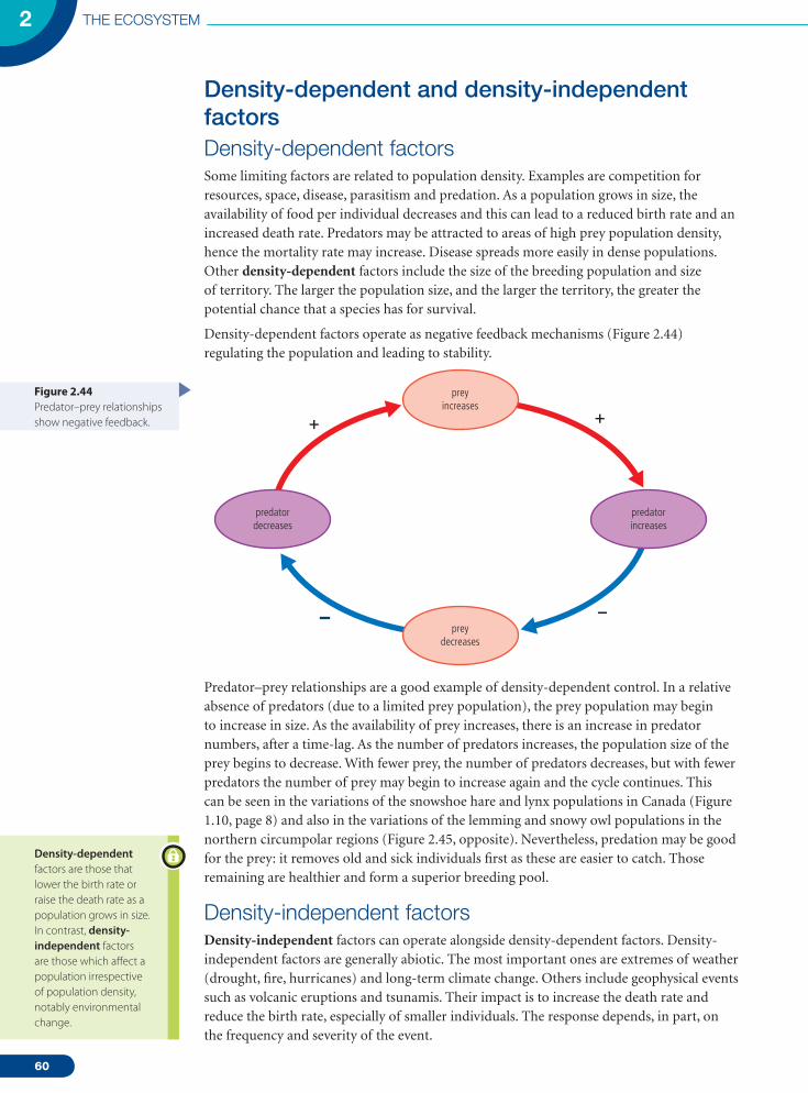
60

THE ECOSYSTEM2

Density-dependent and density-independent factorsDensity-dependent factorsSome limiting factors are related to population density. Examples are competition for resources, space, disease, parasitism and predation. As a population grows in size, the availability of food per individual decreases and this can lead to a reduced birth rate and an increased death rate. Predators may be attracted to areas of high prey population density, hence the mortality rate may increase. Disease spreads more easily in dense populations. Other density-dependent factors include the size of the breeding population and size of territory. The larger the population size, and the larger the territory, the greater the potential chance that a species has for survival.

Density-dependent factors operate as negative feedback mechanisms (Figure 2.44) regulating the population and leading to stability.

prey increases

prey decreases

– –

+ +

predator increases

predator decreases

Predator–prey relationships are a good example of density-dependent control. In a relative absence of predators (due to a limited prey population), the prey population may begin to increase in size. As the availability of prey increases, there is an increase in predator numbers, after a time-lag. As the number of predators increases, the population size of the prey begins to decrease. With fewer prey, the number of predators decreases, but with fewer predators the number of prey may begin to increase again and the cycle continues. This can be seen in the variations of the snowshoe hare and lynx populations in Canada (Figure 1.10, page 8) and also in the variations of the lemming and snowy owl populations in the northern circumpolar regions (Figure 2.45, opposite). Nevertheless, predation may be good for the prey: it removes old and sick individuals first as these are easier to catch. Those remaining are healthier and form a superior breeding pool.

Density-independent factorsDensity-independent factors can operate alongside density-dependent factors. Density-independent factors are generally abiotic. The most important ones are extremes of weather (drought, fire, hurricanes) and long-term climate change. Others include geophysical events such as volcanic eruptions and tsunamis. Their impact is to increase the death rate and reduce the birth rate, especially of smaller individuals. The response depends, in part, on the frequency and severity of the event.

Figure 2.44Predator–prey relationships show negative feedback.

Density-dependent factors are those that lower the birth rate or raise the death rate as a population grows in size. In contrast, density-independent factors are those which affect a population irrespective of population density, notably environmental change.

02_M02_14_82.indd 60 15/04/2010 08:57

61

0

2

4

6

8

10

num

ber o

f ow

ls an

d le

mm

ings

19561950 1951 1952 1953year

1954 1955

lemmings

owls

Internal and external factorsInternal factors include density-dependent fertility or size of breeding territory, and external factors include predation or disease.

The ultimate causes of population regulation are found in the environment: factors external to the population limit the rate at which individuals can reproduce and survive. These factors can be divided into physical and biological classes. The physical class of environmental factors include water availability, nutrient availability, temperature, and so on. The biological factors include predation and competition. Competition can be between species (interspecific competition) or within the same species (intraspecific competition).

Increasingly, human activities have had an impact on natural populations. Farming, settlement, transport and industry have all disrupted natural populations. Humans may cause population growth by removing previous limitations, or cause population decline by creating new stresses.

Four ways that humans can cause population growth:• increase available resources (e.g. by farming; by nutrient pollution in lakes)• reduce competition (e.g. by poisoning insect pests)• reduce pressure from predators (e.g. by over-hunting large carnivores)• introduce animals to new areas (e.g. game releases).

Four ways that humans can cause population decline and extinction:• change the physical environment and cause habitat disruption (e.g. by draining a

swamp; by causing toxic pollution)• change the biological environment by introducing new species (e.g. rabbits in Australia;

rats on islands)• overkill (e.g. big-game hunting)• cause secondary extinctions (e.g. loss of food species).

The environmental damage inflicted by hurricane Katrina in 2005 was widespread. About 85 000 barrels of crude oil escaped from an oil plant in Chalmette, Louisiana, and a further 68 000 barrels were spilled by a damaged storage tank in Venice. The oil pollution from Katrina is among the worst ever in US history. More than 6.5 million gallons of crude oil was spilt in seven major incidents. This figure does not include petrol and oil spilt from up to 250 000 cars that were submerged, or from petrol stations. In addition, more than 500 sewerage systems were damaged across Louisiana. Some 6600 petrol stations, each with an average of three underground storage tanks, as well as hundreds of industrial facilities, were damaged.

Damage to the oyster, crab and shrimp populations was extensive. The Gulf is home to more than 80 per cent of oysters grown in the United States and is the centre of the shrimp industry. In addition, the accumulated long-term industrial pollution held in the soil was released by the floodwaters. Much was pumped into Lake Pontchartrain. The ecology is definitely being changed.

Human impact, both direct and indirect, on the world’s rainforest is having a major effect on species survival. Uncontrolled hunting for bushmeat is removing large species and creating an ‘empty forest syndrome’ – the trees are there but the large species have disappeared. The replacement of natural tropical rainforest by oil palm plantations is replacing a diverse ecosystem with a monoculture ecosystem. In addition, the impact of climate change is a major threat to the rainforest. As many tropical species evolved in environments that had little temperature variation, they may be ill-equipped to deal with changes of more than 3 °C. By 2100, 75 per cent of tropical forests will be warmer than today.

Figure 2.45Variations in the populations of lemmings and snow owls.

02_M02_14_82.indd 61 15/04/2010 08:57

62

THE ECOSYSTEM2

A range of ecological impacts were caused by the Boxing Day 2004 tsunami. The force of the tsunami drove approximately 100 000 tonnes of water onto every 1.5 m of coastline and therefore caused considerable erosion in some parts and devastating deposition in others. The intrusion of salt water has polluted fresh water sources and farmland sometimes as far as several kilometres inland. Coral reefs were damaged, and large area of mangrove uprooted. Of particular concern are the endangered sea turtles of Sri Lanka and some of the Indian islands. On the east coast of Sri Lanka, almost all of the hatcheries were destroyed when the sandy beaches were washed away.

The introduction of a few pairs of European rabbits into Australia (for hunting) resulted in a population explosion to around 600 million animals. In 1950, the government sanctioned the release of the myxomatosis virus – a density-independent factor – and cut the population to 100 million.

However, by 1991, genetic resistance had rebuilt the population to as many as 300 million, prompting a second virus, the calicivirus, to be released. Where there was a greater density of rabbits, the virus was more lethal than where the population was lighter – thus this viral disease illustrates density-dependent control.

Survivorship curves – r- and K-strategistsSlow growing organisms tend to be limited by the carrying capacity of an environment (K), and so are known as K-strategists or K-species. They inhabit stable environments. Species characterized by periods of rapid growth followed by decline, tend to inhabit unpredictable, rapidly changing environments and are termed opportunistic species. They have a fast rate of increase (r) and are called r-strategists or r-species. Many species lie in between these two extremes and are known as C-strategists or C-species.

Species characterized as r-strategists produce many, small offspring that mature rapidly. They receive little or no parental care. Species producing egg-sacs are a good example. In contrast, species that are K-strategists produce very few, often very large offspring that mature slowly and receive much parental support. Elephants and whales are good examples. As a result of the low birth rate, K-strategists are vulnerable to high death rates and extinction.

K-strategists are slow growing and produce few, large offspring that mature slowly; r-strategists grow and mature quickly and produce many, small offspring.

r- and K- selection theoryThis theory states that natural selection may favour individuals with a high reproductive rate and rapid development (r-strategists) over those with lower reproductive rates but better competitive ability (K-strategists). Characteristics of the classes are shown in Table 2.1.

tablE 2.1 A coMPArIsoN of r- ANd K-sPecIes

r-strategists K-strategists

initial colonizers dominant species

large numbers of a few species diverse range of species

highly adaptable generalists

rapid growth and development slow development

early reproduction delayed reproduction

short life longer living

small size larger size

very productive less productive

A female cane toad spawns twice a year and produces up to 35 000 eggs each time!

02_M02_14_82.indd 62 15/04/2010 08:57

63

In predictable environments – those in which resources do not fluctuate – there is little advantage to rapid growth. Instead, natural selection favours species that can maximize use of natural resources and which produce only a few young which have a high probability of survival. These K-strategists have long life spans, large body size and develop slowly.

In contrast, disturbed habitats with rapidly changing conditions favour r-strategists that can respond rapidly, develop quickly and have early reproduction. This leads to a high rate of productivity. Such colonizer species often have a high dispersal ability to reach areas of disturbance.

Species can have traits of both K- and r-strategists. Studies of dandelions in a disturbed lawn had high reproduction rates whereas those on an undisturbed lawn produced fewer seeds but were better competitors.

Survivorship curvesRates of mortality vary with age, size and sometimes gender. Survivorship curves shows changes in survivorship over the lifespan of the species (Figure 2.46).

1

10

100

1000

num

ber o

f ind

ivid

uals

surv

ivin

g

1000 50percentage of life span

K-strategists

C-strategists

r-strategists

Factors that influence survivorship rates include:• competition for resources• adverse environmental conditions • predator–prey relationships.

The two extreme examples of a survivorship curve (as shown in Figure 2.46) are:• the curve for a species where almost all individuals survive for their potential life span,

and then die almost simultaneously (K-strategists) – salmon and humans are excellent examples

• the curve for a species where most individuals die at a very young age but those that survive are likely to live for a very long time (r-strategists) – turtles and oysters are very good examples.

Figure 2.46Survivorship rates.

Examiner’s hint:Note that the scale in Figure 2.47 is semi-logarithmic. This means that one axis – here, the horizontal or x-axis – is a normal scale and the gaps between each unit are regular: the distance between 0 and 50 is the same as between that between 50 and 100. In contrast, the vertical or y-axis is logarithmic.

Note that on the logarithmic scale:• the scale does not start at 0 (in this example, it starts at 1)• the scale goes up in logarithms (the first cycle goes up in 1s, the second cycle in 10s, the next in 100s).

The reason for using a logarithmic scale is that it enables us to show very large values on the same graph as very small values.

02_M02_14_82.indd 63 15/04/2010 08:57

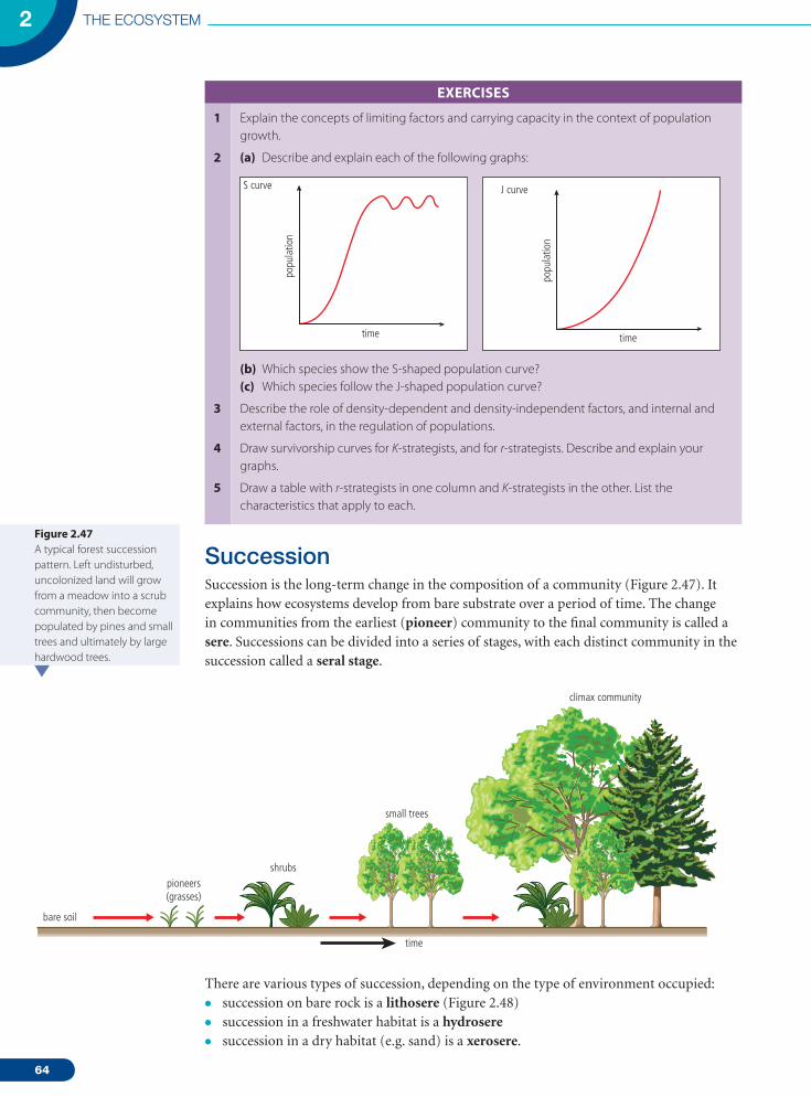
64

THE ECOSYSTEM2

EXERCIsEs

1

2

3

4

5

Explain the concepts of limiting factors and carrying capacity in the context of population growth.

(a) Describe and explain each of the following graphs:

popu

latio

n

time

S curve

popu

latio

n

time

J curve

popu

latio

n

time

S curve

popu

latio

n

time

J curve

(b) Which species show the S-shaped population curve?(c) Which species follow the J-shaped population curve?

Describe the role of density-dependent and density-independent factors, and internal and external factors, in the regulation of populations.

Draw survivorship curves for K-strategists, and for r-strategists. Describe and explain your graphs.

Draw a table with r-strategists in one column and K-strategists in the other. List the characteristics that apply to each.

SuccessionSuccession is the long-term change in the composition of a community (Figure 2.47). It explains how ecosystems develop from bare substrate over a period of time. The change in communities from the earliest (pioneer) community to the final community is called a sere. Successions can be divided into a series of stages, with each distinct community in the succession called a seral stage.

Figure 2.47A typical forest succession pattern. Left undisturbed, uncolonized land will grow from a meadow into a scrub community, then become populated by pines and small trees and ultimately by large hardwood trees.

time

bare soil

pioneers(grasses)

shrubs

small trees

climax community

There are various types of succession, depending on the type of environment occupied:• succession on bare rock is a lithosere (Figure 2.48)• succession in a freshwater habitat is a hydrosere• succession in a dry habitat (e.g. sand) is a xerosere.

02_M02_14_82.indd 64 15/04/2010 08:57

65

bare rock

colonization by lichens, weathering rock and production of dead organic material

growth of moss, further weathering, and the beginnings of soil formation

growth of small plants such as grasses and ferns, further improvement in soil

larger herbaceous plants can grow in the deeper and more nutrient-rich soil

climax community dominated by shrubs and trees

Succession occurring on a previously uncolonized substrate (e.g. rock) is called a primary succession. Secondary succession occurs in places where a previous community has been destroyed (e.g. after forest fires). Secondary succession is faster than a primary succession because of the presence of soil and a seed bank.

Succession happens when species change the habitat they have colonized and make it more suitable for new species. For example, lichens and mosses are typical pioneer species. Very few species can live on bare rock as it contains little water and has few available nutrients. Lichens can photosynthesize and are effective at absorbing water, so they need no soil to survive and are excellent pioneers. Once established, they trap particles blown by the wind; their growth reduces wind speed and increases temperature close to the ground. When they die and decompose they form a simple soil in which grasses can germinate. The growth of pioneers helps to weather parent rock adding still further to the soil. Other species, such as grasses and ferns that grow in thin soil, are now better able to colonize.

The new species are better competitors than the earlier species; for example, grasses grow taller than mosses and lichen, so they get more light for photosynthesis. Their roots trap substrate thereby halting erosion, and they have a larger photosynthetic area, so they grow faster. The next stage involves the growth of herbaceous plants (e.g. dandelion and goosegrass), which require more soil to grow but which out-compete the grasses – they have wind-dispersed seeds and rapid growth, so they become established before larger plants. Shrubs then appear (e.g. bramble, gorse, and rhododendron), which are larger plants that can grow in good soil, and which are better competitors than the slower-growing pioneers.

The final stage of a succession is the climax community. Here grown trees produce too much shade for the shrubs, which are replaced by shade-tolerant forest floor species. The amount of organic matter increases as succession progresses because as pioneer and subsequent species die out, their remains contribute to a build-up of litter from the biomass. Soil organisms move in and break down litter, leading to a build up of organic matter in the soil making it easier for other species to colonize. Soil also traps water, and so increasing amounts of moisture are available to plants in the later stages of the succession.

Figure 2.48A model of succession on bare rock.

02_M02_14_82.indd 65 15/04/2010 08:57

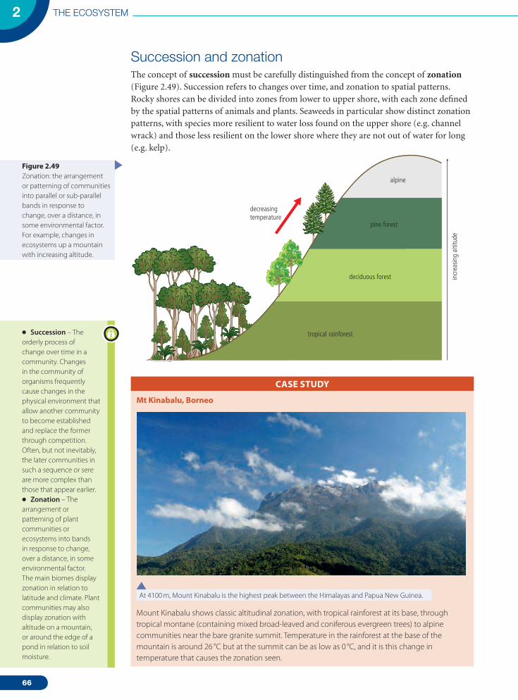
66

THE ECOSYSTEM2

Succession and zonationThe concept of succession must be carefully distinguished from the concept of zonation (Figure 2.49). Succession refers to changes over time, and zonation to spatial patterns. Rocky shores can be divided into zones from lower to upper shore, with each zone defined by the spatial patterns of animals and plants. Seaweeds in particular show distinct zonation patterns, with species more resilient to water loss found on the upper shore (e.g. channel wrack) and those less resilient on the lower shore where they are not out of water for long (e.g. kelp).

decreasing temperature

alpine

pine forest

deciduous forest

tropical rainforest

incr

easin

g al

titud

e

CasE study

mt Kinabalu, borneo

At 4100 m, Mount Kinabalu is the highest peak between the Himalayas and Papua New Guinea.

Mount Kinabalu shows classic altitudinal zonation, with tropical rainforest at its base, through tropical montane (containing mixed broad-leaved and coniferous evergreen trees) to alpine communities near the bare granite summit. Temperature in the rainforest at the base of the mountain is around 26 °C but at the summit can be as low as 0 °C, and it is this change in temperature that causes the zonation seen.

Figure 2.49Zonation: the arrangement or patterning of communities into parallel or sub-parallel bands in response to change, over a distance, in some environmental factor. For example, changes in ecosystems up a mountain with increasing altitude.

•Succession – The orderly process of change over time in a community. Changes in the community of organisms frequently cause changes in the physical environment that allow another community to become established and replace the former through competition. Often, but not inevitably, the later communities in such a sequence or sere are more complex than those that appear earlier.•Zonation – The arrangement or patterning of plant communities or ecosystems into bands in response to change, over a distance, in some environmental factor. The main biomes display zonation in relation to latitude and climate. Plant communities may also display zonation with altitude on a mountain, or around the edge of a pond in relation to soil moisture.

02_M02_14_82.indd 66 15/04/2010 08:57

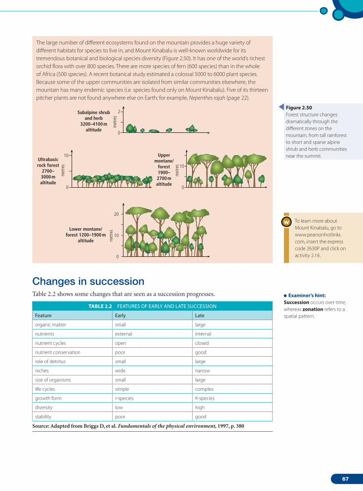
67

The large number of different ecosystems found on the mountain provides a huge variety of different habitats for species to live in, and Mount Kinabalu is well-known worldwide for its tremendous botanical and biological species diversity (Figure 2.50). It has one of the world’s richest orchid flora with over 800 species. There are more species of fern (600 species) than in the whole of Africa (500 species). A recent botanical study estimated a colossal 5000 to 6000 plant species. Because some of the upper communities are isolated from similar communities elsewhere, the mountain has many endemic species (i.e. species found only on Mount Kinabalu). Five of its thirteen pitcher plants are not found anywhere else on Earth; for example, Nepenthes rajah (page 22).

0

2Subalpine shruband herb

3200–4100 maltitude

0

10Ultrabasicrock forest

2700–3000 maltitude

0

met

res

met

res

met

res

met

res 10

Uppermontane/

forest1900–2700 maltitude

0

10

20

Lower montane/forest 1200–1900 m

altitude

Changes in successionTable 2.2 shows some changes that are seen as a succession progresses.

tablE 2.2 feAtures of eArLY ANd LAte successIoN

feature early Late

organic matter small large

nutrients external internal

nutrient cycles open closed

nutrient conservation poor good

role of detritus small large

niches wide narrow

size of organisms small large

life cycles simple complex

growth form r-species K-species

diversity low high

stability poor good

Source: Adapted from Briggs D, et al. Fundamentals of the physical environment, 1997, p. 380

Figure 2.50Forest structure changes dramatically through the different zones on the mountain, from tall rainforest to short and sparse alpine shrub and herb communities near the summit.

To learn more about Mount Kinabalu, go to www.pearsonhotlinks.com, insert the express code 2630P and click on activity 2.16.

Examiner’s hint:succession occurs over time, whereas zonation refers to a spatial pattern.

02_M02_14_82.indd 67 15/04/2010 08:57

68

THE ECOSYSTEM2

Gross productivity, net productivity and diversity will change over time as an ecosystem goes through succession. In the early stages of succession, gross productivity is low due to the initial conditions and low density of producers. The proportion of energy lost through community respiration (i.e. respiration of all organisms present) is relatively low too, so net productivity is high (e.g. the system is growing and biomass is accumulating). As succession progresses, soils become better structured and more fertile, and can support a greater diversity of producers, as well as larger producers. Gross productivity by producers therefore increases. As plants grow, the number of niches increases, food webs become more complex, and diversity increases. As food webs become more complex, net productivity increases. Gross primary productivity, net primary productivity and diversity stabilize as the ecosystem reaches climax population.

Further changes in a succession are shown in Figure 2.51.

Production : respiration ratioWe have seen how early stages of a succession have low GPP but high NPP due to the low overall rates of respiration. This relationship can be described as a ratio (production : respiration or P/R). If production is equal to rate of respiration, the value is 1. Where P/R is greater than 1, biomass accumulates; where P/R is less than 1, biomass is depleted. Where P/R = 1 a steady-state community results. In the later stages of a succession, with an increased consumer community, rates of community respiration are high. Gross productivity may be high in a climax community but, as this is balanced by respiration, the net productivity approaches zero (NP = GP – respiration), and the P/R ratio approaches 1.

If the production : respiration ratios of a food production system are compared to a natural ecosystem with a climax community, clear differences can be seen (Figure 2.52). This diagram compares intensive crop production with deciduous woodland. Fields and woodland both have low initial productivity, which increases rapidly as biomass accumulates. Farmers do not want the P/R ratio to reach 1 because, at that point, community respiration negates the high rates of gross productivity, which means that yields are not increased. The wheat is therefore harvested before P/R = 1. Community respiration is also controlled in the food production system by isolating herbivores and thereby increasing net productivity and growth. In natural woodland, the consumer community increases, so naturally high productivity is balanced by consumption and respiration. The woodland reaches its climax community when P/R = 1 (i.e. all woodland productivity is balanced by respiration).

plant cover and species diversity increases

16th century coastline

little sea sea

100 metres

West

East

soil depth and humus content increases

soil acidity increases

decreasing blown sand movement

increasing moisture availability for plants

woodland scrub heather dunes grass dunes

dune slacks

Figure 2.51Changes in biotic and abiotic factors along a sand-dune succession.

Examiner’s hint:• Early stages of succession – Gross productivity is low; the proportion of energy lost through community respiration is also low, so net productivity is high; the system is growing and biomass is accumulating.• Later stages of succession – With an increased consumer community, gross productivity may be high; however, this is balanced by respiration, so net productivity approaches zero and the production : respiration (P/R) ratio approaches 1.

02_M02_14_82.indd 68 15/04/2010 08:57

69

P/R

ratio

time

climax woodland

agricultural crop

Climax communitiesEcosystem stability refers to how well an ecosystem is able to cope with changes. As we saw in Chapter 1, most ecosystems are negative feedback systems – they contain inbuilt checks and balances without which they would spiral out of control, and no ecosystem would be self-sustaining. Ecosystems with more feedback mechanisms are more stable than simple ecosystems. Thus, ecosystems in the later stages of succession are likely to be more stable because food webs are more complex (because of high species diversity). This means that a species can turn to alternative food sources if one species is reduced. By late succession, large amounts of organic matter are available to provide a good source of nutrients. Nutrient cycles are closed and self-sustaining; they are not dependent on external influences. This also contributes to stability.

The features of a climax community (compared to an early community) are:• greater biomass• higher levels of species diversity• more favourable soil conditions (e.g. greater organic content)• better soil structure (therefore, greater water retention)• lower pH• taller and longer-living plant species • more K-strategists or fewer r-strategists• greater community complexity and stability• greater habitat diversity• steady-state equilibrium.

Figure 2.52Difference in production : respiration ratios between natural and agricultural systems.

Lowland tropical rainforest is a climax community in South-East Asia. Hardwood trees of the family Dipterocarpaceae are dominant. They are often very tall and provide a rich three-dimensional architecture to the forest.

02_M02_14_82.indd 69 15/04/2010 08:57

70

THE ECOSYSTEM2

PlagioclimaxClimatic and edaphic factors determine the nature of a climax community. Human factors frequently affect this process through disturbance. The interference halts the process of succession so that the climax community is not reached. Interrupted succession is known as plagioclimax. An example is the effect of footpath erosion caused by continued trampling by feet. Or consider a sand dune ecosystem, where walkers might trample plants to the extent that they are eventually destroyed.

Human activity can affect the climax community through agriculture, hunting, clearance, burning, and grazing: all these activities create a plagioclimax by arresting succession.

Temperate forests are often dominated by a single tree species, such as the oak.

Redwood forests along the Pacific coast of the USA contain some of the tallest trees in the world. The dominant species in terms of biomass is Sequoia sempervirens. Trees can reach up to 115.5 m (379.1 ft) in height and 8 m (26 ft) in diameter.

Burning and deforestation of the Amazon forest to make grazing land leads to loss of large areas of rainforest. Continued burning and clearance, and the establishment of grasslands, prevents succession occurring.

02_M02_14_82.indd 70 15/04/2010 08:57

71

Deforestation is having a major impact on one of the most diverse biomes, tropical rainforest (Figures 2.53, 2.54 and 2.55). An area of rainforest the size of a football pitch is destroyed every four seconds. As well as loss of habitat and destruction of a complex climax community, the carbon dioxide released when the trees are burnt returns to the atmosphere: this amount of carbon dioxide is more than that from the entire global transport sector (Chapter 6).

Large parts of the UK were once covered by deciduous woodland. Some heather would have been present in the north, but relatively little. From the Middle Ages onwards, forests were cleared to supply timber for fuel, housing, construction of ships (especially oak), and to clear land for agriculture. As a result, soil deteriorated and heather came to dominate the plant community. Sheep grazing has prevented the re-growth of woodland by destroying young saplings.

Controlled burning of heather also prevents the re-establishment of deciduous woodland. The heather is burnt after 15 years, before it becomes mature. If the heather matured, it would allow colonization of the area by other plants. The ash adds to the soil fertility and the new heather growth that results increases the productivity of the ecosystem.

Figure 2.53Deforestation in the Brazilian Amazon basin fluctuates but remains high despite warnings about the consequences for the planet. The loss of the highly diverse climax community and its replacement by agricultural or grazing ecosystems affects global biodiversity, regional weather, the water cycle and sedimentation patterns.

0

5 000

35 000

30 000

25 000

20 000

15 000

10 000sq k

m d

efor

esta

ted,

per

yea

r

20081988 1990 1992 1994 1996 1998 2000 2002 2004 2006year

02_M02_14_82.indd 71 15/04/2010 08:57

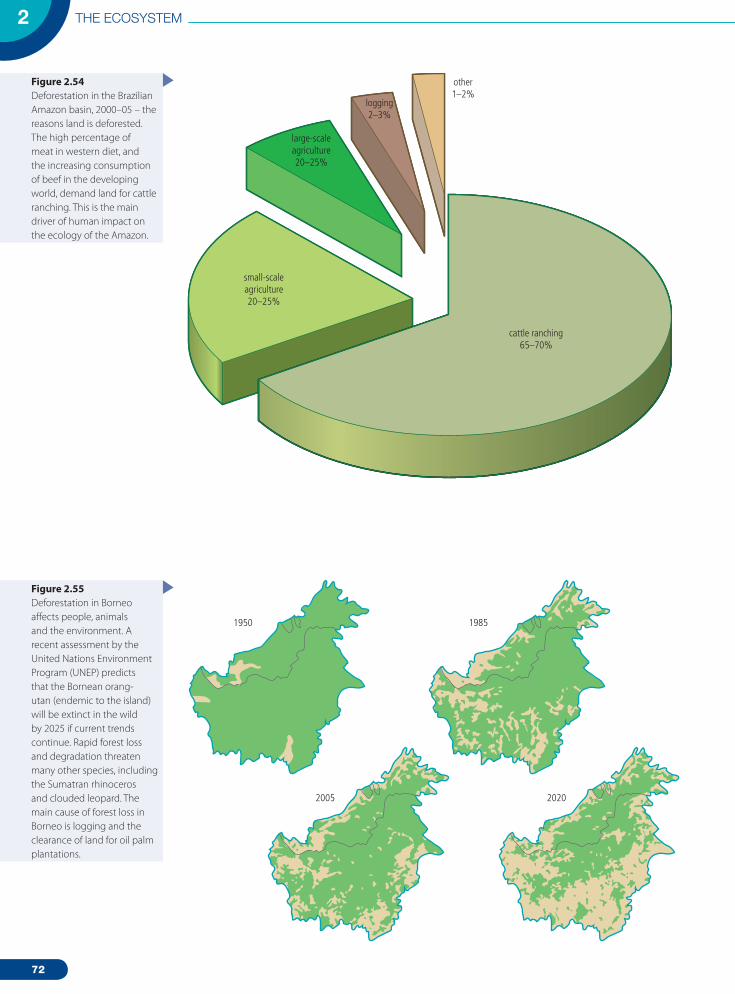
72

THE ECOSYSTEM2

cattle ranching 65–70%

small-scale agriculture 20–25%

large-scale agriculture 20–25%

logging 2–3%

other 1–2%

1950 1985

2005 2020

Figure 2.54Deforestation in the Brazilian Amazon basin, 2000–05 – the reasons land is deforested.The high percentage of meat in western diet, and the increasing consumption of beef in the developing world, demand land for cattle ranching. This is the main driver of human impact on the ecology of the Amazon.

Figure 2.55Deforestation in Borneo affects people, animals and the environment. A recent assessment by the United Nations Environment Program (UNEP) predicts that the Bornean orang-utan (endemic to the island) will be extinct in the wild by 2025 if current trends continue. Rapid forest loss and degradation threaten many other species, including the Sumatran rhinoceros and clouded leopard. The main cause of forest loss in Borneo is logging and the clearance of land for oil palm plantations.

Assessment statements2.7.1 Describe and evaluate methods for measuring changes in abiotic and biotic

components of an ecosystem along an environmental gradient.2.7.2 Describe and evaluate methods for measuring changes in abiotic and biotic

components of an ecosystem due to a specific human activity.2.7.3 Describe and evaluate the use of Environmental Impact Assessments (EIAs).

02_M02_14_82.indd 72 15/04/2010 08:57

73

EXERCIsEs

1

2

3

4

What changes occur along a succession? What impact do these changes have on biodiversity?

What is the P/R ratio? What does it measure? How does the P/R ratio change from early to late succession?

What are the characteristics of climax communities? Your answer should include details of biomass levels, species diversity, soil conditions, soil structure, pH, community complexity, type of equilibrium, and habitat diversity.

What is a plagioclimax, and how are they formed? Give four examples of how human activities lead to the creation of a plagioclimax.

2.7 Measuring changes in the system

Assessment statements2.7.1 Describe and evaluate methods for measuring changes in abiotic and biotic

components of an ecosystem along an environmental gradient.2.7.2 Describe and evaluate methods for measuring changes in abiotic and biotic

components of an ecosystem due to a specific human activity.2.7.3 Describe and evaluate the use of Environmental Impact Assessments (EIAs).

Describe and evaluate methods for measuring change along an environmental gradientEcological gradients are often found where two ecosystems meet (e.g. on beaches or on lake shores) or where an ecosystem suddenly ends (e.g. at forest edges). In these situations, both biotic and abiotic factors vary with distance and form gradients in which trends can be recorded. The techniques used in sampling ecological gradients are based on the quadrat method and, as such, are more easily done on vegetation and immobile or slow-moving animals.

Because environmental variables change along the gradient, random quadrat sampling is not appropriate. All parts of the gradient need to be sampled, so a transect is used. The simplest transect is a line transect – a tape measure laid out in the direction of the gradient (e.g. on a beach this would be at 90° to the sea). All organisms touching the tape are recorded. Many line transects need to be taken to obtain valid quantitative data. Larger samples can be taken from a transect by using a belt transect. This is a band of chosen width (usually between 0.5 and 1 m) laid along the gradient (Figure 2.56).

start

species 1 species 2 species 3

finish

Figure 2.56Belt transects sample a strip through the sample area. Replication of transects is needed to obtain valid quantitative data.

02_M02_14_82.indd 73 15/04/2010 08:57

74

THE ECOSYSTEM2

In both line and belt transects, the whole transect can be sampled (a continuous transect) or samples are taken at points of equal distance along the gradient (an interrupted transect). If there is no discernable vertical change in the transect, horizontal distances are used (e.g. along a shingle ridge succession), whereas if there is a climb or descent then vertical distances are normally used (e.g. on a rocky shore).

It is important that transects are carried out, as far as possible, at the same time of day, so abiotic variables are comparable. Seasonal fluctuations also mean that samples should be taken either as close together in time as possible or throughout the whole year: datalogging equipment allows the latter to take place, although this may be impractical in school studies.

So that data are reliable, and quantitatively valid, transects should be repeated – at least three times is recommended. To avoid bias in placing the transects, a random number generator can be used (page 332). A tape measure is laid at right angles to the environmental gradient: transects are located at random intervals along the tape (Figure 2.57).

first transect randomly located

sample area

subsequent transectslocated systematically

Describe and evaluate methods for measuring changes in abiotic and biotic components of an ecosystem due to a specific human activity Nuclear contamination following the Chernobyl disasterTable 2.3 shows how nuclear accidents are rated worldwide.

EnvIRonmEntal phIlosophIEs

Greater awareness of environmental issues has caused environmental philosophies to alter over time. What would not have been seen as a problem in the past (e.g. mining activity) is now understood to produce toxins and to lead to environmental damage. Greater understanding of scientific issues has influenced public perception of human effects on the environment, and has changed worldviews.

Figure 2.57All transects can be located randomly or, they can be systematically located following the random location of the first. So, for example, subsequent transects might be located every 10 metres along a line perpendicular to the ecological gradient.

02_M02_14_82.indd 74 15/04/2010 08:57

75

tablE 2.3 tHe INterNAtIoNAL NucLeAr eveNt scALe

Level description criteria example

7 major accident • External release of a large amount of radioactive material. Such an event would have acute health affects, delayed health effects over a large area, and long-term environmental consequences.

Chernobyl 1986

6 serious accident •External release of radioactive material requiring emergency countermeasures. Kyshtym (Russian Federation) 1957

5 accident with off-site risk

•External release of radioactive material requiring partial emergency measures.• Severe damage to the nuclear facility – fire or explosion releasing nuclear material

within the facility.

Windscale, UK 1957Three Mile Island, USA 1979

4 accident without significant off-site risk

•External release of radioactivity resulting in the need for local food control.•Significant damage to the nuclear facility.• Overexposure to one or more workers causing a high probability of an early

death.

Windscale, UK 1973

3 serious incident •External release of radioactive material.•On-site events causing a health risk.•Incidents which could lead to further accidents.

2 incident •A failure in safety procedure but no external risk.•A worker is placed at risk; precautions need to be taken.

1 anomaly • Outside normal operating levels.

Chernobyl is located on the Pripyat River, about 100 km north of Kiev (Ukraine) and 140 km south of Gomel (Belarus). Four nuclear reactors were located there, one of which exploded in April 1986. A combination of factors and circumstances contributed to the disaster. First, there were design drawbacks with the reactor. Second, human error, as a result of poor supervision, led to unstable operations.

The result was an increase in thermal power on 26 April 1986 which led to two non-nuclear explosions in quick successions. These penetrated the nuclear reactor and blew the roof off the reactor building. Concrete, graphite and other debris heated to very high temperatures then escaped to the atmosphere.

Radionuclides, normally contained within the reactor core, were released into the atmosphere for nearly 10 days. Widespread distribution of airborne radionuclides resulted across western Europe. This resulted in the contamination of soil, plants and animals, leading to contamination of foodstuffs.

Responding to the hazardThe first response to the incident was the arrival of firefighters from the nearby town of Pripyat. Firefighters fought the fire at very close quarters and all received serious radiation doses. It took over three hours to extinguish all the main fire sites, with the exception of the fire in the core of the reactor. This was achieved by dumping 5000 tonnes of sand, lead and clay by helicopter onto the reactor.

There were 31 deaths and over 200 cases of radiation burns. The health effects of the disaster are still emerging. For example, a sharp increase in throat cancers has been recorded.

In order to isolate the exposed reactor, a sarcophagus (coffin) was built around it. However, due to the difficult working conditions, there are gaps in the container, although these are regularly monitored for radiation. More than a decade later, in September 1997, the EU pledged £75 million to make the sarcophagus safe. An international team had found it in dire need of repairs to prevent radiation leakage.

02_M02_14_82.indd 75 15/04/2010 08:57

76

THE ECOSYSTEM2

The nearby town of Pripyat was closed and the residents were advised to stay indoors. It was later decided to evacuate everybody living within 30 km of the reactor. After the evacuation, decontamination work began. All soil to a depth of 15 cm was removed, and all buildings had to be cleaned. These measures were later found to be of limited effectiveness.

To prevent the contaminated land being washed away, and to prevent radionuclides seeping into rivers and the Kiev reservoir, 140 dykes and dams were built. A large concrete wall was constructed around the plant to prevent radionuclides passing into the soil water and groundwater. In addition, a channel was created to prevent contaminated water getting into the River Dnepr and downstream into drinking sources.

Further afield, the deposition of radioactive material varied. Many places had less than 1 kBq m–2 whereas others had in excess of 100 kBq m–2. This lead to wide variations in the contamination of foods.

The Russian authorities at first denied internationally that there had been a problem at Chernobyl. They were reluctant to admit observers or release information. Scientists in Finland and Sweden used satellites to track the cloud of radioactive isotopes, notably caesium and iodine. Rainfall caused the caesium and iodine to be flushed out of the atmosphere and onto pastureland; it was monitored by scientists in countries affected by the radioactive fall-out. Dosimeters are used to measure radiation and measurements were provided at microroentgens per hour at ground level. Satellites are still used to monitor flooding in the Pripyat river because floodwaters release radon from the groundwater.

Satellite imagesAnother way of measuring change is by using satellite images as shown in the photos below. This method is very reliable, covers a large area and allows us to see change over time. Its visual nature is useful for motivating action.

To learn more about how to manage radiation, go to www.pearsonhotlinks.com, insert the express code 2630P and click on activity 2.17.

To learn more about measuring change with satellite images, go to www.pearsonhotlinks.com, insert the express code 2630P and click on activity 2.18.

These images show deforestation and the development of settlement and farming areas.

02_M02_14_82.indd 76 15/04/2010 08:57

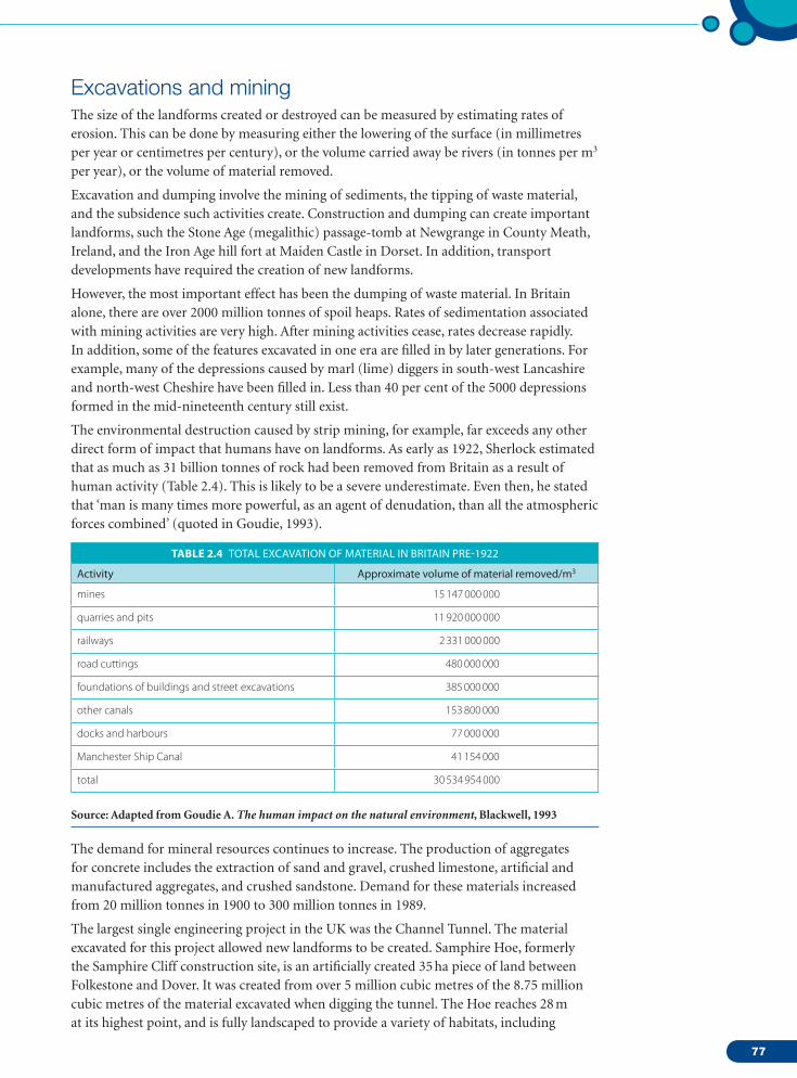
77

Excavations and miningThe size of the landforms created or destroyed can be measured by estimating rates of erosion. This can be done by measuring either the lowering of the surface (in millimetres per year or centimetres per century), or the volume carried away be rivers (in tonnes per m3 per year), or the volume of material removed.

Excavation and dumping involve the mining of sediments, the tipping of waste material, and the subsidence such activities create. Construction and dumping can create important landforms, such the Stone Age (megalithic) passage-tomb at Newgrange in County Meath, Ireland, and the Iron Age hill fort at Maiden Castle in Dorset. In addition, transport developments have required the creation of new landforms.

However, the most important effect has been the dumping of waste material. In Britain alone, there are over 2000 million tonnes of spoil heaps. Rates of sedimentation associated with mining activities are very high. After mining activities cease, rates decrease rapidly. In addition, some of the features excavated in one era are filled in by later generations. For example, many of the depressions caused by marl (lime) diggers in south-west Lancashire and north-west Cheshire have been filled in. Less than 40 per cent of the 5000 depressions formed in the mid-nineteenth century still exist.

The environmental destruction caused by strip mining, for example, far exceeds any other direct form of impact that humans have on landforms. As early as 1922, Sherlock estimated that as much as 31 billion tonnes of rock had been removed from Britain as a result of human activity (Table 2.4). This is likely to be a severe underestimate. Even then, he stated that ‘man is many times more powerful, as an agent of denudation, than all the atmospheric forces combined’ (quoted in Goudie, 1993).

tablE 2.4 totAL excAvAtIoN of MAterIAL IN BrItAIN Pre-1922

Activity Approximate volume of material removed/m3

mines 15 147 000 000

quarries and pits 11 920 000 000

railways 2 331 000 000

road cuttings 480 000 000

foundations of buildings and street excavations 385 000 000

other canals 153 800 000

docks and harbours 77 000 000

Manchester Ship Canal 41 154 000

total 30 534 954 000

Source: Adapted from Goudie A. The human impact on the natural environment, Blackwell, 1993

The demand for mineral resources continues to increase. The production of aggregates for concrete includes the extraction of sand and gravel, crushed limestone, artificial and manufactured aggregates, and crushed sandstone. Demand for these materials increased from 20 million tonnes in 1900 to 300 million tonnes in 1989.

The largest single engineering project in the UK was the Channel Tunnel. The material excavated for this project allowed new landforms to be created. Samphire Hoe, formerly the Samphire Cliff construction site, is an artificially created 35 ha piece of land between Folkestone and Dover. It was created from over 5 million cubic metres of the 8.75 million cubic metres of the material excavated when digging the tunnel. The Hoe reaches 28 m at its highest point, and is fully landscaped to provide a variety of habitats, including

02_M02_14_82.indd 77 15/04/2010 08:57

78

THE ECOSYSTEM2

three ponds. The Hoe is protected from wave erosion by a sea wall of almost 225 000 m3 of concrete. Access to the Hoe is through a 130 m tunnel, itself created as part of the 1974 Channel Tunnel project.

Environmental Impact AssessmentsDemand for resources, for new housing, for new energy supplies and for new transport links are inevitable, but before any development project gets permission to begin, an Environmental Impact Assessment (EIA) must be carried out. The purpose of an EIA is to establish the impact of the project on the environment. It predicts possible impacts on habitats, species and ecosystems, and helps decision makers decide if the development should go ahead. An EIA also addresses the mitigation of potential environmental impacts associated with the development. The report should provide a non-technical summary at the conclusion so that lay-people and the media can understand the implications of the study.

Some countries incorporate EIAs within their legal framework, with penalties and measures that can be taken if the conditions of the EIA are broken, whereas other countries simply use the assessment to inform policy decisions. In some countries, the information and suggestions of the EIA are often ignored, or take second place to economic concerns.

The first stage of an EIA is to carry out a baseline study. This study is undertaken because it is important to know what the physical and biological environment is like before the project starts so that it can be monitored during and after the development. Variables measured as part of a baseline study should include:• habitat type and abundance – record total area of each habitat type• species list – record number of species (faunal and flora) present• species diversity – estimate the abundance of each species and calculate diversity of the

community• list of endangered species• land use – assess land use type and use coverage• hydrology – assess hydrological conditions in terms of volume, discharge, flows, and

water quality• human population – assess present population• soil – quality, fertility, and pH.

EnvIRonmEntal phIlosophIEs

EIAs offer advice to governments, but whether or not they are adopted depends on the environmental philosophy of the government involved. In China, for example, the EIA for the Three Gorges Dam showed the damage that would be done to the environment, but the government chose to focus on the benefits to the country.

It is often difficult to put together a complete baseline study due to lack of data, and sometimes not all of the impacts are identified. An EIA may be limited by the quality of the baseline study. The value of EIAs in the environmental decision-making process can be compromised in other ways. Environmental impact prediction is speculative due to the complexity of natural systems and the uncertainty of feedback mechanisms thus making environmental decisions more difficult: the predictions of the EIA may, therefore, prove to be inaccurate in the long term. On the other hand, at their best, EIAs can lead to changes in the development plans, avoiding negative environmental impact. It could be argued that any improvement to a development outweighs any negative aspects.

To learn more about how EIAs are applied in the UK, go to www.pearsonhotlinks.com, insert the express code 2630P and click on activity 2.19.

02_M02_14_82.indd 78 15/04/2010 08:57

79

CasE study

three Gorges dam, yangtze River

The Three Gorges Dam is the largest hydroelectric dam development in the world. Located on the Yangtze River in the People’s Republic of China (Figure 2.58), construction began in 1993 and the dam was fully operational by the end of 2009. Project engineers have estimated that the dam could generate an eighth of the country’s electricity. This energy will be produced without the release of harmful greenhouse gases. The Chinese government cite other improvements that the development produces: reduced seasonal flooding and increased economic development along the edges of the new reservoir.

CHINA

Beijing

Fengjie

ThreeGorges Dam

Chongqing

Yangtze River

YangtzeRiver

An EIA was required to look at potential ecosystem disruption; relocation of people in areas to be flooded, and the social consequences of resettlement; the effects of sedimentation in areas behind the dam which would have reduced water speed; the effects of landslides from the increase in geological pressure from rising water; and earthquake potential.

Case study continued

The Three Gorges Dam is one and a half miles wide and more than 600 feet high. On completion, it created a reservoir hundreds of feet deep and nearly 400 miles long.

Figure 2.58Location of the Three Gorges Dam. As well as affecting the immediate area of the reservoir formed, the river is affected upstream by changes in the flow of the Yangtze, and downstream by changes in siltation.

02_M02_14_82.indd 79 15/04/2010 08:58

80

THE ECOSYSTEM2

The EIA determined that there are 47 endangered species in the Three Gorges Dam area, including the Chinese river dolphin and the Chinese sturgeon. The report identified economic problems as well as the environmental problems that disruption of the ecosystem would cause. For example, the physical barrier of the dam would interfere with fish spawning and, in combination with pollution, that would have a serious impact on the fishing economy of the Yangtze River. In terms of social costs, the dam would flood 13 cities, 140 towns, 1352 villages, and 100 000 acres of China’s most fertile land. Two million people would have had to be resettled by 2012, and 4 million by 2020. Geological problems included the growing risk of new landslides and increased chance of earthquakes (due to the mass of water in a reservoir altering the pressure in the rock below), and a reduction in sedimentation reaching the East China Sea (reducing the fertility of the land in this area).

The overall view of the people responsible for the development was that the environmental and social problems did not reduce the feasibility of the project, and that the positive impact on the environment and national economy outweighed any negative impact.

EXERCIsEs

1

2

Describe methods for measuring changes along an environmental gradient. Divide these into abiotic and biotic factors. Evaluate each – what are the limitations of each and how will they affect the data you collect?

Find your own example of an EIA. What were the conclusions of the study? Were the recommendations followed?

pRaCtICE QuEstIons

1

2

The figure below shows a food web for a small-scale ecosystem.

(a) State which trophic level is occupied by the bats. [1]

(b) Describe two impacts of a reduction in stream invertebrates on the food web of the ecosystem. [2]

© International Baccalaureate Organization [2008]

(a) State two functions of producers in an ecosystem. [2]

(b) For a named ecosystem, draw a food chain with named species showing three appropriately labelled trophic levels. [3]

(c) Distinguish between a pyramid of biomass and a pyramid of productivity. [2]

© International Baccalaureate Organization [2008]

To learn more about the Three Gorges Dam, go to www.pearsonhotlinks.com, insert the express code 2630P and click on activity 2.20.

02_M02_14_82.indd 80 15/04/2010 08:58

81

3

4

Simpson’s diversity index states that: D = N(N 2 1) ________

n(n 2 1) where N = the total number of individuals

of all species found and n = the number of individuals of a particular species.

A garden pond contains the following organisms

Animal type Number of individualsgoldfish 24

carp 5

frogs 6

water boatmen 1500

water snail 1200

water flea 2500

Using the Simpson diversity index formula above, calculate the diversity of this pond. [3]© International Baccalaureate Organization [2004]

The table and graphs below show population data for the mayfly (Ephemerella subvaria) in two similar streams, A and B, in Minnesota, USA. Data were collected on population size (number of mayfly m−2) and mean mass of mayfly between September 1970 and June 1971.

populatIon dynamICs oF mayFly In stREams a and b

stream A stream B

Month No. of mayfly / m–2

Mean biomass / g m–2

Mean mass of mayfly / mg

No. of mayfly / m–2

Mean biomass / g m–2

Mean mass of mayfly / mg

Sept 6530 1.4 0,2 5251 1.2 0.2

Oct 4432 4.6 1.0 2001 1.3 0.6

Nov 4082 6.6 1.6 905 0.7 0.8

Dec 4053 10.8 2.6 400 0,4 1.1

Jan 3660 13.0 3.5 123 0.2 1.7

Feb 2007 12.8 6.3 99 0.2 2.4

Mar 1587 18.4 11.6 98 0.3 3.2

Apr 230 4.9 21.5 80 0.9 11.4

May 84 1.8 22.4 34 0.3 10.6

June 44 1.0 23.6 24 0.4 20.0

(a) (i) Using the data from the table and graphs, describe the relationship between population size and mean mass for mayfly in stream A. [2]

(ii) Outline two differences in the populations of stream A and stream B during the study period. [2]

(iii) Calculate the percentage change in the population of mayfly in stream A from September to June. [1]

02_M02_14_82.indd 81 15/04/2010 08:58

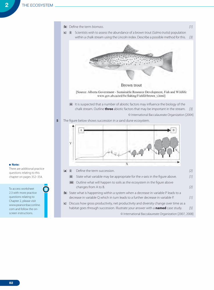
82

THE ECOSYSTEM2

5

(b) Define the term biomass. [1]

(c) (i) Scientists wish to assess the abundance of a brown trout (Salmo trutta) population within a chalk stream using the Lincoln index. Describe a possible method for this. [3]

(ii) It is suspected that a number of abiotic factors may influence the biology of the chalk stream. Outline three abiotic factors that may be important in the stream. [3]

© International Baccalaureate Organization [2004]

The figure below shows succession in a sand dune ecosystem.

(a) (i) Define the term succession. [2]

(ii) State what variable may be appropriate for the x-axis in the figure above. [1]

(iii) Outline what will happen to soils as the ecosystem in the figure above changes from A to B. [2]

(b) State what is happening within a system when a decrease in variable P leads to a decrease in variable Q which in turn leads to a further decrease in variable P. [1]

(c) Discuss how gross productivity, net productivity and diversity change over time as a habitat goes through succession. Illustrate your answer with a named case study. [5]

© International Baccalaureate Organization [2007, 2008]

note:There are additional practice questions relating to this chapter on pages 352–354.

To access worksheet 2.3 with more practice questions relating to Chapter 2, please visit www.pearsonbacconline.com and follow the on-screen instructions.

02_M02_14_82.indd 82 15/04/2010 08:58