biostatistics methods for translational & clinical researchchap/ss05-day2-designs-partb.pdf ·...

BIOSTATISTICS METHODS FOR TRANSLATIONAL & CLINICAL RESEARCH

DESIGNING CLINICAL RESEARCH Part B: Statistical Issues

Relative Risk & Odds Ratio

Suppose that each subject in a large study, at a particular time, is classified as positive or negative according to some risk factor, and as having or not having a certain disease under investigation. For any such categorization the population may be enumerated in a 2x2 table, as follows:

TotalFactor Yes (+) No (-)Exposed (+) A B A + BUn-exposed (-) C D C + DTotal A + C B + D N = A + B + C + D

Disease

The entries A, B, C and D in the table are sizes of the four combinations of disease presence-and-absence and factor presence-and-absence and the number N at the lower right corner of the table is the total population size. The relative risk is

TotalFactor Yes (+) No (-)Exposed (+) A B A + BUn-exposed (-) C D C + DTotal A + C B + D N = A + B + C + D

Disease

B)C(AD)A(C

DCC

BAARR

++

=

+÷

+=

B)C(AD)A(C

DCC

BAARR

++

=

+÷

+=

In many situations, the number of subjects classified as disease positive is very small as compared to the number classified as disease negative, that is,

BBADDC

≅+≅+

B/DA/C

C/DA/BBCADRR

==

≅

B/DA/C

C/DA/BBCADRR

==

≅

The resulting ratio, AD/BC, is an approximate relative risk, but it is often referred to as odds ratio because

A/B and C/D are the odds in favor of having disease from groups with or without the factor;

A/C and B/D are the odds in favor of having exposed to the factors from groups with or without the disease.

The two odds, A/C and B/D, can be easily estimated in case-control studies, by using sample frequencies, a/c and b/d.

Modeling a Proportion

n,1,iki2i1ii )}x,,x,x;{(y:form the in are data Regression

=

In “regular” Regression Model, we impose the condition that Y is on the continuous scale – We even assume that Y is normally distributed with a constant variance.

We impose the condition that Y is on the continuous scale maybe because of the “normal error model” - not because Y is always on the continuous scale. In a variety of applications, the Dependent Variable of interest may have only two possible outcomes, and therefore can be represented by an Binary or Indicator Variable Y taking on values 0 and 1. Let: π = Pr(Y=1)

Let Y be the Dependent Variable Y taking on values 0 and 1, and: π = Pr(Y=1) Y is said to have the “Bernouilli distribution” (Binomial with n = 1). We have:

π)π(1Var(Y)πE(Y)

−==

Consider, for example, a study of Drug Use among middle school kids, as a function of gender and age of kid, family structure (e.g. who is the head of household), and family income. In this study, the dependent variable Y was defined to have two possible outcomes: (i) Kid uses drug (Y=1), and (ii) Kid does not use drug (Y=0).

In another example, say, a man has a physical examination; he’s concerned: Does he have prostate cancer? The “truth” would be confirmed by a biopsy. But it’s a very painful process (at least, could we say if he needs a biopsy?) In this study, the dependent variable Y was defined to have two possible outcomes: (i) Man has prostate cancer (Y=1), and (ii) Man does not have prostate cancer (Y=0). Possible predictors include PSA level, age, race.

Or in a case-control study, the response variable is the “disease” – a binary indicator, often code as 0/1.

The basic question is: Can we do “regression” when the dependent variable, or “response”, is binary?

For “binary” Dependent Variables, we run into problems with the “Normal Error Model” – The distribution of Y is Bernouilli. However, the “normal” assumption is not very important (i.e. “robust”); effects of any violation is quite minimal – especially if n is large!

The Mean of Y is in well-defined but it has limited range: Mean of Y = Pr(Y=1) = π 0≤ π ≤1, and fitted values may fall outside of (0,1). However, that’s a minor problem.

The Variance (around the regression line) is not constant (a model violation that we learn in diagnostics); variance is function of the Mean π of Y (which is a function of predictors): σ2 = π(1- π)

More important, the relationship is not linear. For example, with one predictor X, we usually have:

X

Y

0

1

XXX XX X X X

X X X X XXXXXXX

In other words, We still can focus on “modeling the mean”, in this case it is a Probability, π = Pr(Y=1), but the usual linear regression with the “normal error regression model” is definitely not applicable – all assumptions are violated, some may carry severe consequences.

So, what should we do? We have to get out of that limited range (0,1); we need some transformation of (binary variable) Y

EXAMPLE: Dose-Response Data in the table show the effect of different concentrations of (nicotine sulphate in a 1% saponin solution) on fruit flies; here X = log(100xDose), just making the numbers easier to read. Dose(gm/100cc) # of insects, n # killed, r x p (%)

0.1 47 8 1.000 17.00.15 53 14 1.176 26.40.2 55 24 1.301 43.60.3 52 32 1.477 61.50.5 46 38 1.699 82.60.7 54 50 1.845 92.6

0.95 52 50 1.978 96.2

Proportion p is an estimate of Probability π

UNDERLYING ASSUMPTION It is assumed that each subject/fly has its own tolerance to the drug. The amount of the chemical needed to kill an individual fruit fly, called “individual lethal dose” (ILD), cannot be measured - because only one fixed dose is given to a group of n flies (indirect assay) (1) If that dose is below some particular fly’s ILD, the insect survived. (2) Flies which died are those with ILDs below the given fixed dose.

INTERPRETATION OF DATA • 17% (8 out of n=47) of the

first group respond to dose of .1gm/100cc (x=1.0); that means 17% of subjects have their ILDs less than .1

• 26.4% (14 out of n=53) of the 2nd group respond to dose of .15gm/100cc (X=1.176); that means 26.4% of subjects have their ILDs less than .15

• we view each dose D (with X = logD) as upper endpoint of an interval and p the cumulative relative frequency.

Dose # n # killed X p(%)0.1 47 8 1.000 17.0

0.15 53 14 1.176 26.40.2 55 24 1.301 43.60.3 52 32 1.477 61.50.5 46 38 1.699 82.60.7 54 50 1.845 92.6

0.95 52 50 1.978 96.2

A symmetric sigmoid dose-response curve suggests that it be seen as some cumulative distribution function (cdf).

“Empirical evidence”, i.e. data, suggest that we view p the cumulative relative frequency. This leads to a “transformation” from “π” to an “upper endpoint”, say Y* (which is on the continuous scale) corresponding to that cumulative frequency of some cdf. After this transformation, the regression model is then imposed on Y*, transformed value of π

Let π be the probability “to be modeled” and X a covariate (let consider only one X for simplicity). The first step in the regression modeling process is to obtain “the equivalent deviate Y* of π” using the following transformation:

.function density yprobabilit some is f(z)

f(z)dzor f(z)dzπ*

*

Y

Y

∫∫∞

∞−=

MODELING A PROBABILITY

Cumulative Proportion π

1- π

Transformation: π to Y* which is on a linear scale

As a result, the proportion π has been transformed into a variable Y* on the “linear” or continuous scale with unbounded range. We can use Y* as the dependent variable in a regression model. (We now should only worry about “normality” which is not very important)

The relationship between covariate X (in the example, log of the dose) or covariates X’s and Probability π (through Y) is then stipulated by the usual simple linear regression:

∑=

+=

+=

k

1iii0

*

10*

xββY

regression multipleor xββY

:

∫∫∞

∞−=

*)(or

Ydzzf

*Y

*

f(z)dzπ

:through Y to πtranslate toorder in f(.)function" density yprobabilit" a is need we All

In theory, any probability density function can be used. We can choose one either by its simplicity and/or its extensive scientific supports. And we can check to see if the data fit the model (however, it’s practically hard because we need lots of data to tell).

A VERY SIMPLE CHOICE

0z ;ef(z):density with

on"Distributi lExponentiaUnit " is ypossibilit A

z ≥= −

Result (for one covariate X) is:

xββlnπor ;e

dzeπ

10

xββ

xββ

z

10

10

+==

=

+

∞

−−

−∫

That is to model the “log” of the probability as a “linear function” of covariates.

The advantage of the approach of modeling the “log” of the probability as a “linear function” of covariates, is easy interpretation of model parameters, the probability is changed by a multiple constant (i.e.“multiplicative model” which is usually plausible)

REGRESSION COEFFICIENTS

• If X1 is binary (=0/1) representing an exposure, β1 represents the (log of) the “odds” (of having the event represented by Y) associated with the exposure – adjusted for that of X2

• If X1 is on a continuous scale, β1 represents the (log of) the “odds” (of having the event represented by Y) associated with one unit increase in the value of X1 - adjusted for X2

Besides the Unit Exponential probability density, one can also use of the Standard Normal density in the transformation of π:

A HISTORICAL CHOICE

)2θexp(

2π1f(θ(

:density Normal Standard the is f""

f(θ(θ)π

2

y

0

*

−=

= ∫

This “Probit Transformation” leads to the “Probit Model”; Y* is called the “probit” of π. The word “probit” is a shorten form of the phrase “PROBability unIT” (but it is not a probability), it is a standard normal variate.

The Probit Model was popular in years past and had been used almost exclusively to analyze “bioassays” for many decades. However, there is no closed-form formula for Y* (it’s not possible to derive an equation relating π to x without using an integral sign):

∫+

−=x

d10

0

2

)2

exp(21ββ

θθπ

π

LOGISTIC TRANSFORMATION

2exp(θxp[1exp(θxf(θ(

:density with onDistributi Logistic (Standard)

+=

Result is:

x)ββexp(11

x)βexp(β1x)βexp(β

dθ]e[1

eπ

10

10

10

βxβY

2θ

θ0*

−−+=

+++

=

+= ∫

+=

∞−

xββπ1

πlog

eπ1

πe11π1

e1eπ

10

xββ

xββ

xββ

xββ

10

10

10

10

+=−

=−

+=−

+=

+

+

+

+

We refer to this as “Logistic Regression”

Exponential transformation leads to a linear model of “Log of Probability”: ln(π); Logistic transformation leads to a linear model of “Log of Odds”: ln[π/(1- π)] – also called “logit”

When π is small (rare disease/event), probability and the odds are approximately equal.

Odds1Oddsπ

π1πOdds

+=

−=

Advantages:

(1) Also very simple data transformation: Y = log{p/(1-p)}

(2) The logistic density, with thicker tails as compared to normal curve, may be a better representation of real-life processes (compared to Probit Model which is based on the normal density).

A POPULAR MODEL • Although one can use the Standard Normal

density in the regression modeling process (or any density function for that purpose),

• The Logistic Regression, as a result of choosing Logistic Density remains the most popular choice for a number of reasons: closed form formula for π, easy computing (Proc LOGISTIC)

• The most important reasons: interpretation of model parameter and empirical supports!

REGRESSION COEFFICIENTS

• If X1 is binary (=0/1) representing an exposure, β1 represents the (log of) the “odds ratio” (of having the event represented by Y) associated with the exposure – adjusted for that of X2

• If X1 is on a continuous scale, β1 represents the (log of) the “odds ratio” (of having the event represented by Y) associated with one unit increase in the value of X1 - adjusted for X2

)(Ratio Odds

lnln

ln:(exposed) 1

ln:)(unexposed 01

ln

binary is XSay :

1

exp

exp

1expexp

2210exp1

220exp1

22110

1

β

β

βββ

ββ

βββπ

π

eOddsOdds

OddsOddsxOddsxxOddsx

xx

osedun

osed

osedunosed

osed

osedun

==

=−

++==

+==

++=−

Example

β1 is the odds ratio on the log scale if X is binary

Logistic Regression applies in both prospective and retrospective (case-control) designs. In prospective design, we can calculate/estimate the probability of an event (for specific values of covariates). In retrospective design, we cannot calculate/estimate the probability of events because the “intercept” is meaningless but relationship between event and covariates are valid.

SUPPORTS FOR LOGISTIC MODEL The fit and the origin of the linear logistic model could be easily traced as follows. When a dose D of an agent is applied to a pharmacological system, the fractions fa and fu of the system affected and unaffected satisfy the so-called “median effect principle” (Chou, 1976): where ED50 is the “median effective dose” and “m” is a Hill-type coefficient; m = 1 for first-degree or Michaelis-Menten system. The median effect principle has been investigated much very thoroughly in pharmacology. If we set “ π= fa”, the median effect principle and the logistic regression model are completely identical with a slope β1= m.

m

50u

a

EDd

ff

=

PARAMETER ESTIMATION: MLE

0/1y;]xβexp[β1

]}xβ{exp[β

)π(1π

)yPr(YL

:Function Likelihoodβx)exp(α1x)βexp(βπ

:Model

i

n

1i i10

yi10

y1n

1ii

yi

i

n

1ii

10

i

ii

=++

+=

−=

==

+++

=

∏

∏

∏

=

−

=

=

An Application: Quantal Assays

Indirect Assays: Dose fixed, Response random.

Depending on the “measurement scale” for the response (our random variable), we divide indirect assays into two groups:

(1) Quantal assays, where the response is binary: whether or not an event (like the death of the subject) occurs,

(2) Quantitative assays, where measurements for the response are on a continuous scale.

Quantal response assays belong to the class of qualitative indirect assays. They are characterized by experiments in which each level of a stimulus (eg. dose of a drug) is applied to n experimental units; r of them respond and (n-r) do not response.That is “binary” response (yes/no). The group size “n” may vary from dose to dose; in theory, some n could be 1 (so that r = 0 or 1).

THE ASSAY PROCEDURE • The usual design consists of a series of dose

levels with subjects completely randomized among/to the dose levels. The experiment may include a standard and a test preparations; or maybe just the test.

• The dose levels chosen should range from “very low” (few or no subjects would respond) to “rather high” (most or all subjects would respond).

• The objective is often to estimate the LD50; the number of observations per preparation depends on the desired level of precision of its estimate – sample size estimation is a very difficult topic.

The most popular parameter LD50 (for median lethal dose), or ED50 (for median effective dose), or EC50 (for median effective concentration) is the level of the stimulus which result in a response by 50% of individuals in a population. (1) It is a measure of the agent’s potency, which could be used to form relative potency. (2) It is chosen by a statistical reason; for any fixed number of subjects, one would attain greater precision as compared to estimating, say, LD90 or LD10 or any other percentiles.

Inference & Validity

INFERENCES & VALIDITIES • Two major levels of inferences are involved in

interpreting a study, a clinical trial The first level concerns Internal validity; the

degree to which the investigator draws the correct conclusions about what actually happened in the study.

The second level concerns External Validity (also referred to as generalizability or inference); the degree to which these conclusions could be appropriately applied to people and events outside the study.

Truth in The Universe

Truth in The Study

Findings in The Study

Research Question Study Plan Study Data

External Validity Internal Validity

A Simple Example: An experiment on the effect of Vitamin C on the prevention of colds could be simply conducted as follows. A number of n children (the sample size) are randomized; half were each give a 1,000-mg tablet of Vitamin C daily during the test period and form the “experimental group”. The remaining half , who made up the “control group” received “placebo” – an identical tablet containing no Vitamin C – also on a daily basis. At the end, the “Number of colds per child” could be chosen as the outcome/response variable, and the means of the two groups are compared.

Assignment of the treatments (factor levels: Vitamin C or Placebo) to the experimental units (children) was performed using a process called “randomization”. The purpose of randomization was to “balance” the characteristics of the children in each of the treatment groups, so that the difference in the response variable, the number of cold episodes per child, can be rightly attributed to the effect of the predictor – the difference between Vitamin C and Placebo. Randomization helps to assure Internal Validity.

What about External Validity?

For instance, when looked to establish a relationship but found no statistically significant correlation. On this basis it is concluded that there is no relationship between the two factors. How could this conclusion be wrong -- that is, what are the "threats to validity"? A “conclusion” is a generalization from findings of the study to truth in the universe; it involves external validity.

REJECTION • Back to a “Statistical Test”. • The Null Hypothesis H0 is a “Theory”. The

Data are “Reality”. When they do not agree, then we have to trust the reality; That’s when H0 is rejected.

• How do we tell if Theory and Reality do not agree? When the data show overwhelmingly that it is almost impossible to have the data that we already collected if H0 is true (that it is possible but with a very small probability).

ABOUT REJECTIONS

Hypothesis Testing is like Trial by Jury

A very important concept: when a null hypothesis is not rejected it does not necessarily lead to its acceptance, because a “not guilty” verdict is just an indication of “lack of evidence” and “innocence” is just one of its possibilities. That is, when a difference in not statistically significant, there are still two possibilities:

(i)The null hypothesis is true,

(ii)There is not enough evidence from sample data to support its rejection (i.e. not enough data).

Studies may be inconclusive because they were poorly planned, not enough data were collected to accomplished the goals and support the hypotheses. To assure external validity, we have to assure of adequate sample size.

A TYPICAL SCENARIO An investigator wants to randomize mice with induced tumors – say, lung tumors - into two groups; mice in one group receive placebo and the others some new agent – the effect of the new agent is to reduce the size/volume of the tumors. And he/she needs help to figure out the sample sizes.

A TYPICAL “PRODUCT”

A statement such as “with 15 mice per group, we would be able to detect – with a statistical power of 80% - a reduction of 40% in tumor volume using a two-sided two-sample t-test at the 5% level”

Where do we get that 40% tumor volume specified in the Alternative Hypothesis? Whose responsibility, investigator’s or statistician’s?

It’s easier in basic sciences with animal studies: it’s the “dose” – previously determined from a one-arm trial: ED40

It could be a problem when both sides are inexperienced. Sometimes the investigator simply makes up an effect size. Sometimes they take an easy way out: See how much the investigator can afford – say n = 12 per group – then how much we can “see” or detect – a reduction of 27% or 32% etc…

Sample Size Determination

APPROACH TO SAMPLE SIZE • The target of the investigation is a statistic θ; for

example, the difference of two sample means or two sample proportions.

• Consider the statistic θ which often the MLE of some parameter (e.g. the difference of two population means), and assume that it is normally distributed as N(θ0, Σ0

2) under the null hypothesis H0 and as N(θA, ΣA

2) under an alternative hypothesis HA; usually Σ0

2 = ΣA2 or

we can assume this equality for simplification.

| θ0 - θA | = z 1-αΣ0 + z 1-βΣA

MAIN RESULT • We have:

| θ0 - θA | = z 1-αΣ0 + z 1-βΣA where the z’s are percentiles of N(0,1).

• Or if Σ02 = ΣA

2 = Σ, or if we assume this equality for simplification, then ( θ0 - θA )2 = (z 1-α + z 1-β)2 Σ2

• This “the Basic Equation for Sample Size Determination”; and we use z1-α/2 if the statistical test is used as two-sided.

DETECTION OF A CORRELATION

• The Problem: To confirm certain level of correlation between two continuously measured variables

The Null hypothesis to be tested is H0: ρ = ρ0, say ρ = 0.

The Alternative hypothesis to be tested is H0: ρ = ρA , say ρ = .4.

The target statistic is Pearson’s “r”; indirectly through Fisher’s transformation to “z”.

The Coefficient of Correlation ρ between the two random variables X and Y is estimated by the (sample) Coefficient of Correlation r but the sampling distribution of r is far from being normal. Confidence intervals of is by first making the “Fisher’s z transformation”; the distribution of z is normal if the sample size is not too small

3n1(z)σ

ρ1ρ1ln

21E(z)

Normalzr1r1ln

21z

2

−=

−+

=

∈

−+

=

DETECTION A CORRELATION • The null hypothesis to be tested is H0: ρ = 0 • The target statistic is Fisher’s z: • Basic parameters are:

• Result: Total required sample size:

3n1 Σand ;

ρ1ρ1ln

21θ 0;

0101ln

21θ 2

A

AA0 −

=−+

==−+

=

( θ0 - θA )2 = (z 1-α + z 1-β)2 Σ2

2A

2β1α/21

θ)z(z

3n −− ++=

−+

=r1r1ln

21z

RESULTS FOR CORRELATION

• The null hypothesis to be tested is H0: ρ = 0 • The target statistic is Fisher’s z: • Basic parameters are:

• Result: Total required sample size:

• Example: If

3n1 Σand ;

ρ1ρ1ln

21θ 0;

0101ln

21θ 2

A

AA0 −

=−+

==−+

=

2A

2β1α/21

θ)z(z

3n −− ++=

47.424

.84)(1.963n 2

2

≥+

+=

−=→= :powe 80% & sided2 5%for ;424.4. rAA θρ

−+

=r1r1ln

21z

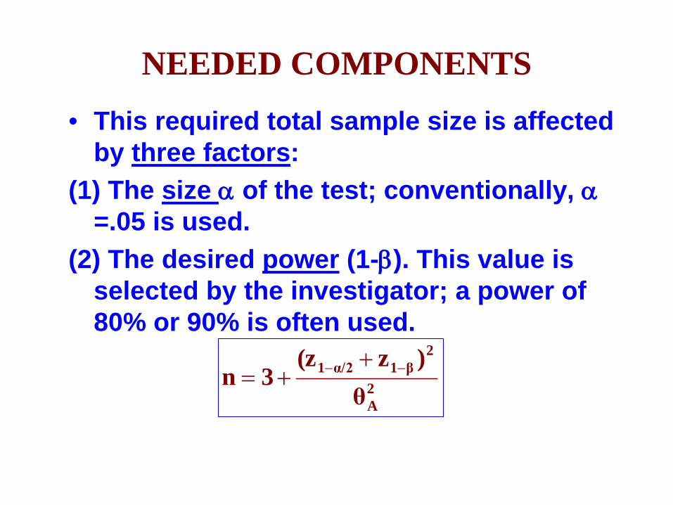
NEEDED COMPONENTS • This required total sample size is affected

by three factors: (1) The size α of the test; conventionally, α

=.05 is used. (2) The desired power (1-β). This value is

selected by the investigator; a power of 80% or 90% is often used.

2A

2β1α/21

θ)z(z

3n −− ++=

(3) The size of the coefficient of correlation to be detected:

It is obvious that the planning sample size is not easy; a good solution requires knowledge of the scientific problem, some good idea of what would be the alternative Hypothesis.

A

AA ρ1

ρ1ln21θ

−+

=

COMPARISON OF TWO MEANS • The Problem: The endpoint is on a continuous

scale; for example, a researcher is studying a drug which is to be used to reduce the cholesterol level in adult males aged 30 and over. Subjects are to be randomized into two groups, one receiving the new drug (group 1), and one a look-alike placebo (group 2). The response variable considered is the change in cholesterol level before and after the intervention.

The null hypothesis to be tested is H0: µ2 - µ1= 0 The target statistic is θ = x2 - x1

DIFFERENCE OF TWO MEANS • The null hypothesis to be tested is H0: µ1 = µ2 • The target statistic is θ = x2 - x1

• Basic parameters are: θ0 = 0, θA = d, and

Or: d2 = (z 1-α + z 1-β)2 Σ2

Nnn4)11( 2

21

22 σσ =+=Σ

( θ0 - θA )2 = (z 1-α + z 1-β)2 Σ2

RESULTS FOR TWO MEANS

• The null hypothesis to be tested is H0: µ1 = µ2 • The target statistic is θ = x2 - x1

• Basic parameters are: θ0 = 0, θA = d, and

• Or: d2 = (z 1-α + z 1-β)2 Σ2

Nnn4)11( 2

21

22 σσ =+=Σ

2

22

11 )(4d

zzN σβα −− +=

NEEDED COMPONENTS • This required total sample size is

affected by four factors: (1) The size α of the test; conventionally,

α =.05 is used. (2) The desired power (1-β). This value is


2

22

11 )(4d


NEEDED COMPONENTS (3) The quantity d, called the "minimum clinical

significant difference”, d = |µ2 - µ1|, (its its determination is a clinical decision, not a statistical decision).

(4) The variance of the population. This variance σ2 is the only quantity which is difficult to determine. The exact value is unknown; we may use information from similar studies or past studies or use some "upper bound".

2

22

11 )(4d


EXAMPLE • Specifications: Suppose a researcher is studying

a drug which is used to reduce the cholesterol level in adult males aged 30 or over, and wants to test it against a placebo in a balanced randomized study. Suppose also that it is important that a reduction difference of 5 be detected (d=5). We decide to preset α =.05 and want to design a study such that its power to detect a difference between means of 5 is 95% (or β =.05). Also, the variance of cholesterol reduction (with placebo) is known to be about σ2 = 36.

• Result:

groupeach in subjects 38or ;765361.65) + 4(1.96N 2

2 ==

COMPARISON OF 2 PROPORTIONS

• The Problem: The endpoint may be on a binary scale. For example, a new vaccine will be tested in which subjects are to be randomized into two groups of equal size: a control (not immunized) group (group 1), and an experimental (immunized) group (group 2). Subjects, in both control and experimental groups, will be challenged by a certain type of bacteria and we wish to compare the infection rates.

The null hypothesis to be tested is H0: π2 - π1 = 0 The target statistic is θ = p2 - p1

DIFFERENCE OF 2 PROPORTIONS • The null hypothesis to be tested is H0: π1 = π2 • The target statistic is θ = p2 - p1

• Basic parameters are: θ0 = 0, θA = d, and approximately

Or d2 = (z 1-α + z 1-β)2 Σ2

Nnn4)1()11)(1(

21

2−−−−

−=+−=Σ ππππ

( θ0 - θA )2 = (z 1-α + z 1-β)2 Σ2

RESULTS FOR 2 PROPORTIONS

• The null hypothesis to be tested is H0: π1 = π2 • The target statistic is θ = p2 - p1

• Basic parameters are: θ0 = 0, θA = d, and approximately

Or d2 = (z 1-α + z 1-β)2 Σ2

Nnn4)1()11)(1(

21

2−−−−

−=+−=Σ ππππ

22

11)1()(4

dzzN

−−

−−−

+=ππ

βα

NEEDED COMPONENTS • This required total sample size is affected by

four factors: • (1) The size α of the test; conventionally, α =.05

is used. • (2) The desired power (1-β). This value is


22

β1α1 dπ)(1π)z4(zN−−

−−−

+=

NEEDED COMPONENTS (3) The quantity d, also called the "minimum clinical

significant difference”, d = | π2 - π1| (its its determination is a clinical decision, not a statistical decision).

(4) π is the average proportion π = (π2 + π1)/2; It is obvious that the planning sample size is more difficult and a good solution requires knowledge of the scientific problem, some good idea of the magnitude of the proportions themselves.

22

β1α1 dπ)(1π)z4(zN−−

−−−

+=

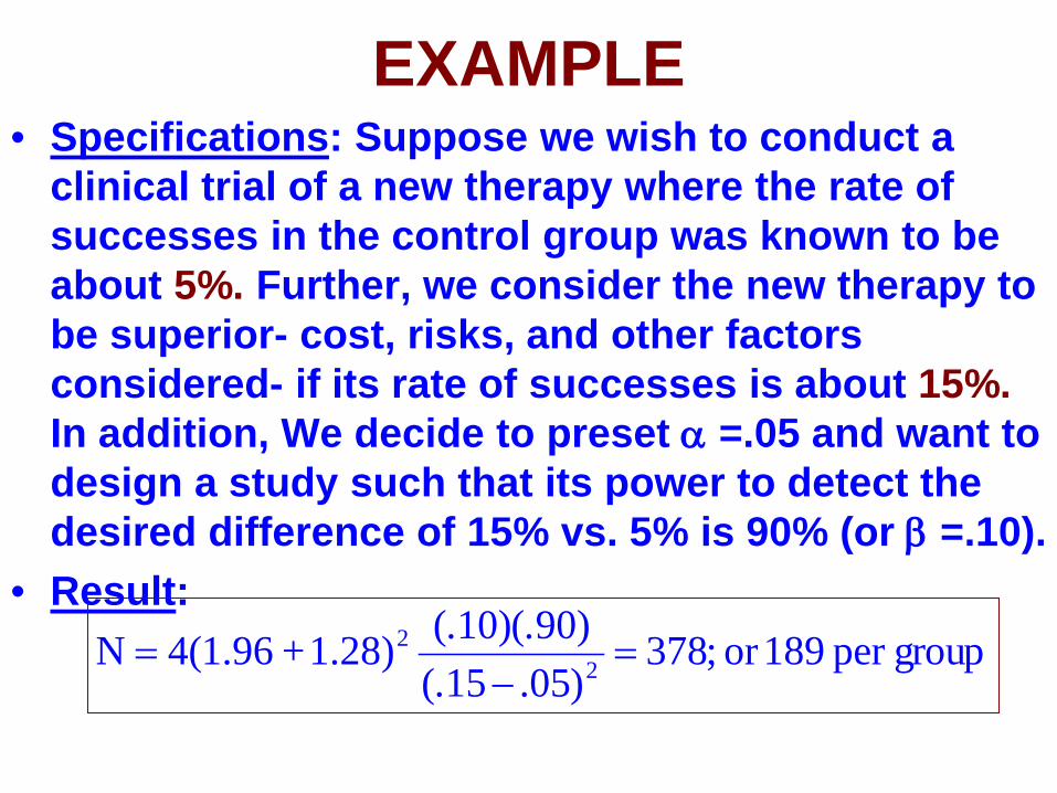
EXAMPLE • Specifications: Suppose we wish to conduct a

clinical trial of a new therapy where the rate of successes in the control group was known to be about 5%. Further, we consider the new therapy to be superior- cost, risks, and other factors considered- if its rate of successes is about 15%. In addition, We decide to preset α =.05 and want to design a study such that its power to detect the desired difference of 15% vs. 5% is 90% (or β =.10).

• Result: groupper 189or ;378

)05.15(.)90)(.10(.1.28) + 4(1.96N 2

2 =−

=

CASE-CONTROL STUDIES

• Both cohort and case-control- are comparative; the validity of the conclusions is based on a comparison.

• In a cohort study, say a clinical trial, we compare the results from the “treatment group” versus the results from the “placebo group”.

• In a case-control study, we compare the “cases” versus the “controls” with respect to an exposure under investigation (“exposure” could be binary or continuous).

DIFFERENT FORMULATION • In a cohort study, for example a two-arm clinical

trial, the decision at the end is based on a “difference”; difference of two means or of two proportions. The “size” of the difference is the major criterion for sample size determination.

• In a case-control study, we compare the exposure histories of the two groups. At the end, we do not search for a difference; instead, the alternative hypothesis of a case-control study is postulated in the form of a relative risk. But the two are related.

CASE-CONTROL DESIGN FOR A BINARY RISK FACTOR

• The data analysis maybe similar to that of a Clinical Trial where we want to compare two proportions.

• However in the design stage, the alternative hypothesis is formulated in the form of a relative risk ρ. Since we cannot estimate or investigate "relative risk" using a case-control design, we would treat the given number ρ as an "odds ratio", the ratio of the odds of being exposed by a case divided by the odds of being exposed by a control.

0

0

1

1

π1π

π1π

ρ

−

−=

CLINICAL SIGNIFICANT DIFFERENCE

• From:

• We solve for the proportion for the cases, and use the previous formula for sample size applies with d = π1 - π0:

0

01 1)π(ρ1

ρππ−+

=

0

0

1

1

π1π

π1π

ρ

−

−=

CASE-CONTROL DESIGN FOR A CONTINUOUS RISK FACTOR

• Data are analyzed using Logistic Regression • The Model is:

• Key Parameter: β1 is the log of the Odds Ratio due to one unit increase in the value of X

xββp1

plnLogit

x)]β(βexp[11x)X|1Pr(Yp

10x

x

10x

+=−

=

+−+====

APPLICATION TO LOGISTIC MODEL

We use the Bayes’ Rule to express the ratio of posterior probabilities as the ratio of prior probabilities times the likelihood ratio:

}0)Y|xPr(X1)Y|xPr(X}{

0)Pr(Y1)Pr(Y{

x)X|0Pr(Yx)X|1Pr(Y

0)0)Pr(YY|xPr(X1)1)Pr(YY|xPr(X

x)X|0Pr(Yx)X|1Pr(Y

====

==

=====

======

=====

THE LOGISTIC MODEL

{)|0Pr()|1Pr(

xXYxXY

====

} = {)0Pr()1Pr(

==

YY

}{)0|Pr()1|Pr(

====

YxXYxX

}

Taking the log of the left-hand side, we obtain the Logistic Regression Model; On the right-hand side: The ratio of prior probabilities is a constant (with respect to x) and the likelihood ratio is the ratio of two pdf’s or two densities.

NORMAL COVARIATE • Assume covariate X is normally distributed

• The log of the Odds Ratio associated with “one standard deviation increase in value of X” is:

220

212

01

220

21

20

021

1

σσσ if)x σμμ(ConstantLogit

)xσ1

σ1()x

σμ

σμ(ConstantLogit

densities) of ln(ratioConstantLogit

==−

+=

−+−+=

+=

σ)(lnρdthat so ;σμμρ ln 01 =

−=

RESULT

2

2β1α1

22

22

β1α1

2

22

β1α1

(logρ)z4(z

σ(logρσ)z4(z

dσ)z4(zN

)

)

−−

−−

−−

+=

+=

+=

EXAMPLE Suppose that an investigator is considering to design a case-control study; its aim is to investigate a potential association between coronary heart disease and serum cholesterol level. Suppose further that it is desirable to detect an odds ratio ρ = 2.0 for a person with cholesterol level 1 standard deviation above for the mean for his or her age group using a two-sided test with a significance level of 5% and a power of 90%.

31/group subjects; 62

1.28)(1.96(ln2)

4

)z(z(ρ

4N

1.28z.10β1.96z.05α

22

2β1α12

β1

α1

≅

+=

+=

=→==→=

−−

−

−

)

A More Interesting & complete illustration:

CROSS-OVER EXPERIMENT DESIGNS

We are now ready to look at a more comprehensive, more advanced, and more interesting example. I choose the “Cross-over Design” which is rather popular in clinical research but, but one reason or another, it is not covered in first-year programs and books. We will consider both binary and continuous outcomes.

Lung cancer is the leading cause of cancer death in the United States and worldwide. Cigarette smoking causes approximately 90% of lung cancer. Despite anti-smoking campaigns over the past 40 years, over 45 million (22%) adult Americans are still current smokers. The development of a viable chemoprevention strategy targeting current smokers potentially could decrease lung cancer mortality.

Previous studies have shown (1) that the tobacco specific nitrosamine 4(methylnitrosamino)-1-(3-pyridyl)-1-butanone (NNK) is a major lung carcinogen in tobacco smoke, (2) that 2-phenethyl isothiocyanate (PEITC) is a potent inhibitor of NNK-induced lung carcinogenesis in rats and mice. So we applied and got a grant to assess, via a placebo-controlled cross-over design, the effect of PEITC supplementation on changes of NNK metabolism in smokers. We hypothesize that there will be a 30% increase in urinary NNAL plus NNAL-Gluc among PEITC treated subjects (taking more toxin out).

THE ROLE OF STUDY DESIGN In a “standard” experimental design, a linear model for a continuous response/outcome is:

+

+

=

ErroralExperiment

EffectTreatment

ConstantOverall

Y

The last component, ‘experimental error”, includes not only error specific to the experimental process but also includes “subject effect” (age, gender, etc…). Sometimes these subject effects are large making it difficult to assess “treatment effect”; given certain level “hypothesized” treatment effect (e.g. Our 30% total NNAL), it would require a much larger sample size – larger than we could afford.

Blocking (to turn a completely randomized design into a randomized complete block design ) would help. But it would only help to “reduce” subject effects, not to “eliminate them: subjects in the same block are only similar, not identical – unless we have “blocks of size one”. And that the basic idea of “Cross-over Designs” – a very special form of “repeated measure designs/studies..

In the most simple cross-over design, subjects are randomly divided into two groups (often of equal sign); subjects in both groups/series take both treatments (experimental treatment and placebo/control) but in different “orders”.

Of course, “order effects” and “carry-over effects” are possible. And the cross-over designs are not always suitable. They are commonly used when treatment effects are not permanent; for example some treatments of rheumatism.

THE DESIGN In our “PEITC trial”, measurements (urinary total NNAL) will be taken from each subject in the two supplementation sequences as seen in the following diagram: Group 1: Period #1 (PEITC; A1) – washout – Period #2 (Placebo; B2) Group 2: Period #1 (Placebo; B1) – washout – Period #2 (PEITC; A2) The letter is used to denote supplementation or treatment (A for PEITC and B for Placebo) and the number, 1 or 2, denotes the period; e.g. “A1” for PEITC taken in period #1.

The “washout periods” are inserted in order to eliminate possible “carry-over effects” (The half-life of dietary PEITC in vivo is between 2-3 hours, with complete excretion within 1-2 days following ingestion) and, in the modeling and analysis, we will have to find a way cancel “order effects” in order assess “treatment effects”. Here and throughout the first part, we consider outcomes on continuous scale.

OUTCOME VARIABLE From the design: Group 1: Period #1 (PEITC; A1) – washout – Period #2 (Placebo; B2) Group 2: Period #1 (Placebo; B1) – washout – Period #2 (PEITC; A2) Our data analysis will be based on the following “outcome variables” (Treatment - Placebo): X1 = A1 - B2; and X2 = A2 - B1 This subtraction will cancel the “within-sequence” effects of all subject-specific factors. This process will result in two independent samples (often with the same or similar sample size if there are no or minimal dropouts or missing data.

Recall the general model: The subtractions X1 = A1 - B2; and X2 = A2 - B1 will cancel not only effects of all subject-specific factors; they cancel the “overall constant” as well, leaving only two components/parameters to be modeled and analyzed: the “treatment effect” (difference between PEITC & Placebo) and the “period (or order) effect” difference between period 1 and period 2).

+

+

=

ErroralExperiment

EffectTreatment

ConstantOverall

Y

A SIMPLE LINEAR MODEL Design: Group 1: Period #1 (PEITC; A1) – washout – Period #2 (Placebo; B2) Group 2: Period #1 (Placebo; B1) – washout – Period #2 (PEITC; A2) Outcome variables: X1 = A1 - B2; and X2 = A2 - B1 There are different ways to express a linear model; a very simple one would be as follows: X1 is normally distributed as N(α+β,σ2) X2 is normally distributed as N(α-β,σ2) In this models, α represents the PEITC supplementation effect (α>0 if and only if PEITC increases the total NNAL) and β represents the period effect (β>0 if and only if measurement from period 1 is larger than from period 2).

(1) The X’s do not really need to have normal distributions; the robustness comes from the fact that our analysis will be based on the normal distribution of the sample mean – not of the data, and the sample mean would be almost normally distribution for moderate to large sample sizes (Central Limit Theorem).

(2) Among the three parameters, α represents the

PEITC effect and is the primary target; we have no interest in the other two (β and σ2). They are nuisance; we have to handle them properly to make inferences on α valid and efficient.

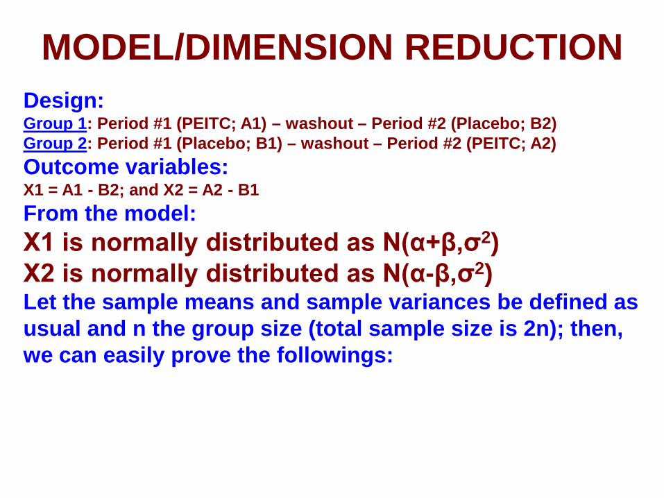
MODEL/DIMENSION REDUCTION Design: Group 1: Period #1 (PEITC; A1) – washout – Period #2 (Placebo; B2) Group 2: Period #1 (Placebo; B1) – washout – Period #2 (PEITC; A2) Outcome variables: X1 = A1 - B2; and X2 = A2 - B1 From the model: X1 is normally distributed as N(α+β,σ2) X2 is normally distributed as N(α-β,σ2) Let the sample means and sample variances be defined as usual and n the group size (total sample size is 2n); then, we can easily prove the followings:

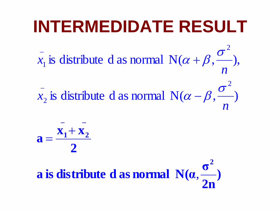
INTERMEDIDATE RESULT

)2nσN(α normal as ddistribute is a

2xxa

2

_

2

_

1

,

),(N normal as ddistribute is

),,(N normal as ddistribute is

2_

2

2_

1

+=

−

+

nx

nx

σβα

σβα

ESTIMATION OF PARAMETERS (1) Estimation of Variance. We can pool data from the two

sequences to estimate the common variance σ2 by sp2

– the same pooled estimate used in two-sample t-test. (2) Estimation of Treatment Effect. Parameter α

representing the PEITC effect, the difference between PEITC and the placebo, is estimated by a – the average of the two sample means. Its 95 percent confidence interval is given by:

Ns

ta p975.±

The t-coefficient goes with (N-2) degrees of freedom; without missing data, N = 2n – total number of subjects.

TESTING FOR TREATMENT EFFECT Testing for PEITC Treatment Effect. Null hypothesis

of “no treatment effects” H0: α = 0 is tested using the “t test”, with (N-2) degrees of freedom:

N/sat

p

=

It’s kind of “one-sample t-test” but we use the degree of freedom associated with sp. Alternatively, one can frame it as a two-sample t-test comparing X1 versus (-X2) as seen from X1 is normally distributed as N(α+β,σ2) X2 is normally distributed as N(α-β,σ2)

ISSUES FOR SAMPLE SIZE

The basis for sample size determination is the “statistic” “a” and its distribution:

from which one obtains distributions under the Null and Alternative Hypotheses.

)2nσN(α normal as ddistribute is a

2xxa

2

_

2

_

1

,

+=

VARIANCE COMPONENTS

[ ]

[ ]:B)r(A, and CV(NNAL) need We

B)r(A,12Var(A)B)2Cov(A,Var(B)Var(A)Var(X)

CV(NNAL)

Var(B)lnNNAL)Var(A2

−=−+=

=

==

Recall that X1 and X2 – each is the difference of two total NNAL - on the log scale; and from the model, X1 is distributed as N(α+β,σ2) and X2 as N(α-β,σ2). We would get to the common variance σ2 by:

Two-period crossover designs are often used in clinical trials in order to improved sensitivity of the trial by eliminating individual patient effects. They have been popular in dairy husbandry studies, long-term agricultural experiments, bioavailability and bioequivalence studies, nutrition experiments, arthritic and periodontal studies, and educational and psychological studies – where treatment effects are not permanent.

The response could be quantitative but quite often, e.g. the response is whether or not relief from pain is obtained, the response variable is binary.

THE DESIGN Recall the following design; the only difference is that, in this case, the four outcomes A1, A2, B1, and B2 are binary – say 1 if positive response and 0 otherwise: Group 1: Period #1 (Trt A; A1) – washout – Period #2 (Trt B; B2) Group 2: Period #1 (Trt B; B1) – washout – Period #2 (Trt A; A2) The washout periods are optional and the group sizes could be different (due to dropouts).

In general, let Y be the outcome or dependent variable taking on values 0 and 1, and: π = Pr(Y=1) Y is said to have the “Bernouilli distribution” (Binomial with n = 1). We have:

)1()()(

πππ

−==

YVarYE

Studies would involve some independent variables (treatment, order, etc…)

THE LOGISTIC MODELS

The Logistic models for cross-over design are ( J. J. Gart, Biometrika 1969):

βαλ

βαλ

βαλ

βαλ

βαλ

βαλ

βαλ

βαλ

i

i

i

i

i

i

i

i

e1e1)Pr(A2;

e1e1)Pr(B1

e1e1)Pr(B2;

e1e1)Pr(A1

−+

−+

+−

+−

++

−−

++

++

+==

+==

+==

+==

In this models, (1) λ‘s represent the subjects effects varying from subject to subject; (2) α represents the PEITC supplementation effect (α>0 if and only if PEITC is more effective) – our main interest - and (3) β represents the period effect (β>0 if and only if a treatment from period 1 is more effective than from period 2).

In this modeling:

(1) We “code’ binary covariates (Treatment and Order) as (+1/-1) instead of (0,1);

(2) All subject-specific covariates are lumped together with the Intercept.

It was shown by Gart (1969) that optimum inferences about treatment and order effects, regarding subjects effects as nuisance, are based on those subjects with unlike responses in two periods; that are subjects whose pair of outcomes are either (0,1) or (1,0). This is similar to the argument leading to the McNemar Chi-square test.

# 1: Period 1 (Trt A; A1) – Period 2 (Trt B; B2) # 2: Period 1 (Trt B; B1) – Period 2 (Trt A; A2)

The analysis will be conditioned on:

A1+B2 = 1, and

B1+A2 = 1

βαλ

βαλ

βαλ

βαλ

βαλ

βαλ

βαλ

βαλ

i

i

i

i

i

i

i

i

e1e1)Pr(A2;

e1e1)Pr(B1

e1e1)Pr(B2;

e1e1)Pr(A1

−+

−+

+−

+−

++

−−

++

++

+==

+==

+==

+==

1)0)Pr(B2Pr(A10)1)Pr(B2Pr(A10)1)Pr(B2Pr(A1

1)B20,Pr(A10)B21,Pr(A10)B21,Pr(A11)B2A1|1Pr(A1

==+====

=

==+====

==+=

β)2(α

β)2(α

e111)A2B1|1Pr(A2

e11

1)0)Pr(B2Pr(A10)1)Pr(B2Pr(A10)1)Pr(B2Pr(A1

1)B20,Pr(A10)B21,Pr(A10)B21,Pr(A11)B2A1|1Pr(A1

−−

+−

+==+=

+=

==+====

=

==+====

==+=

Data: Frequencies of subjects with different Outcomes (0,1) and (1,0)

Treatments (A,B) Treatments (B,A)Oucome A=1 ya1 ya2

Oucome B=1 yb1 yb2

Total n1 n2

Notation: yij; j is the sequence (1if AB and 2 if BA) and i is the treatment with positive outcome.

Note: The same set of data can also be assembled into a different 2x2 Table

Treatments (A,B) Treatments (B,A)1st Outcome=1 ya1 yb2

2nd Outcome =1 yb1 ya2

Total n1 n2

p2e111)A2B1|1Pr(A2

p1e111)B2A1|1Pr(A1

β)2(α

β)2(α

=+

==+=

=+

==+=

−−

+−


Oucome B=1 yb1 yb2

Total n1 n2

Results: With n1 and n2 fixed, ya1 and ya2 are distributed as Binomials B(n1,p1) and B(n2,p2)

Results: With n1 and n2 fixed, ya1 and ya2 are distributed as Binomials B(n1,p1) and B(n2,p2)

(Conditional) Likelihood Function:

b2a2b1a1 yy

a2

2yy

a1

1 p2)(1p2yn

p1)(1p1yn

L −

−

=

β)2(α

β)2(α

e11

e11

−−

+−

+=

+=

2

1

p

p

{ }[ ]

[ ] [ ] 21

a2a1

nα)2(βnβ)2(α

b2b1a2

2

a1

1

y2y

a2

2y1y

a1

1

e1e1

α)(β2yβ)(α2yexpyn

yn

p2)(1p2yn

p1)(1p1yn

L

−+− ++

−++−

=

−

−

=

TREATMENT EFFECT

+==

==

==

b2a2

ba

b1a1

ab

b1a2

b2a1^

b2b1

a2a1^

yyn

yyn

161Var(b)Var(a)

yyyyln

41bβ

yyyyln

41aα

SUGGESTED EXERCISES

#1. When a patient is diagnosed as having cancer of the prostate, an important question in deciding on treatment strategy for the patient is whether or not the cancer has spread to the neighboring lymph nodes. The question is so critical in prognosis and treatment that it is customary to operate on the patient (i.e., perform a laparotomy) for the sole purpose of examining the nodes and removing tissue samples to examine under the microscope for evidence of cancer. However, certain variables that can be measured without surgery may be predictive of the nodal involvement; one of which is level of serum acid phosphatase. Suppose an investigator considers to conduct a case-control study to evaluate this possible relationship between nodal involvement (cases) and level of serum acid phosphatase. Suppose further that it is desirable to detect an odd ratio of θ = 1.5 for an individual with a serum acid phosphatase level of one standard deviation above the mean for his/her age group using a two-sided test with a significance level of 5 percent and a power of 80 percent. Find the total sample size needed for using a two-sided test at the .05 level of significance.

#2. With data in this arrangement, what does an independence between “columns” and “rows” mean and how does it fit in with parameter estimates ?

Treatments (A,B) Treatments (B,A)1st Outcome=1 ya1 yb2

2nd Outcome =1 yb1 ya2

Total n1 n2

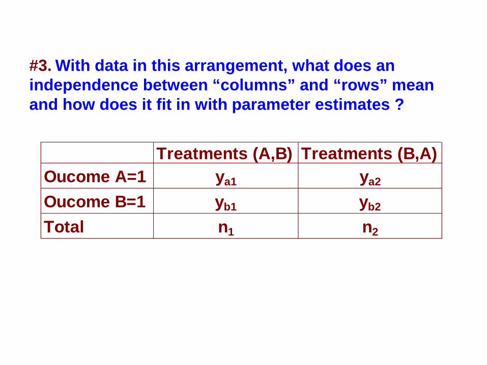
#3. With data in this arrangement, what does an independence between “columns” and “rows” mean and how does it fit in with parameter estimates ?


Oucome B=1 yb1 yb2

Total n1 n2

#4. Back to the case of the PEITC trial, finish the sample size calculation with the following assumptions for NNAL: Coefficient of variation is estimated at 0.6, and Intra-subject correlation is estimated at 0.4.

biostatistics methods for translational & clinical researchchap/ss05-day2-designs-partb.pdf ·...

Documents