biogeosciences carbon and nutrient mixed layer dynamics in the

Biogeosciences, 5, 1395–1410, 2008www.biogeosciences.net/5/1395/2008/© Author(s) 2008. This work is distributed underthe Creative Commons Attribution 3.0 License.

Biogeosciences

Carbon and nutrient mixed layer dynamics in the Norwegian Sea

H. S. Findlay1,*, T. Tyrrell 1, R. G. J. Bellerby2,3, A. Merico4, and I. Skjelvan2,3

1National Oceanography Centre, Southampton, European Way, Southampton, UK2Bjerknes Centre for Climate Research, University of Bergen, Allegaten 55, 5007, Bergen, Norway3Geophysical Institute, University of Bergen, Allegaten 70, 5007, Bergen, Norway4Institute for Coastal Research, Geesthacht, Germany* now at: Plymouth Marine Laboratory, Prospect Place, The Hoe, Plymouth, PL1 3DU, UK

Received: 24 August 2007 – Published in Biogeosciences Discuss.: 14 September 2007Revised: 6 August 2008 – Accepted: 2 September 2008 – Published: 15 October 2008

Abstract. A coupled carbon-ecosystem model is comparedto recent data from Ocean Weather Station M (66◦ N, 02◦ E)and used as a tool to investigate nutrient and carbon processeswithin the Norwegian Sea. Nitrate is consumed by phyto-plankton in the surface layers over the summer; however thedata show that silicate does not become rapidly limiting fordiatoms, in contrast to the model prediction and in contrastto data from other temperate locations. The model estimatesatmosphere-ocean CO2 flux to be 37 g C m−2 yr−1. The sea-sonal cycle of the carbonate system at OWS M resembles thecycles suggested by data from other high-latitude ocean lo-cations. The seasonal cycles of calcite saturation state and[CO2−

3 ] are similar in the model and in data at OWS M: val-ues range from∼3 and∼120µmol kg−1 respectively in win-ter, to∼4 and∼170µmol kg−1 respectively in summer. Themodel and data provide further evidence (supporting previ-ous modelling work) that the summer is a time of high satu-ration state within the annual cycle at high-latitude locations.This is also the time of year that coccolithophore blooms oc-cur at high latitudes.

1 Introduction

The Norwegian Sea (Fig. 1) is an important high latituderegion for processes including uptake and sequestration ofCO2, primary production and large-scale ocean mixing. Aswith many other high latitude locations the mixed layer depthundergoes large seasonal fluctuations forcing seasonal dy-namics of biology and chemistry in the upper ocean (Nilsenand Falck, 2006). High concentrations of nutrients in winter(nitrate>12µmol L−1, phosphate>0.9µmol L−1 and sili-cate>5.5µmol L−1, Dale et al., 1999) are reduced to low

Correspondence to:H. S. Findlay([email protected])

levels in the surface layer by consumption during spring andsummer. Interannual variations in observations give a rangeof nitrate summer concentrations between near 0µmol L−1

and 2µmol L−1 (Kohly, 1998; Haupt et al., 1999, Dale et al.,1999). The lack of full depletion of nitrate in summer at bothOWS M and at (60◦ N, 20◦ W) in the North Atlantic, com-pared to other temperate sites (e.g. NABE, 47◦ N, 20◦ W),has been the subject of much speculation and two main hy-potheses have been put forward to explain this phenomenon:1) diatoms are present in low numbers and are limited byrapid consumption of silicate and hence do not bloom to thesame magnitude as other areas (Dale et al., 1999); 2) largepopulations of micro-zooplankton grazers rapidly consumethe other phytoplankton and prevent them from proliferatingsufficiently to exhaust nitrate (Taylor et al., 1993; Peinert etal., 1989).

The eastern Bering Sea is another high-latitude site thathas been used to investigate the associated dynamics ofplankton and carbonate systems. A detailed understandingof how plankton and the carbonate system interact with eachother in the real ocean is of interest for predicting how theocean will respond to ongoing and future ocean acidifica-tion. Merico et al. (2006)’s model study assessed the possi-ble links between success of the coccolithophoreEmilianiahuxleyiin the natural environment and the ambient values ofcarbonate ion concentration ([CO2−

3 ]) following an earlier in-vestigation addressing which environmental conditions mayhave contributed to the largeE. huxleyiblooms in the easternBering Sea from 1996 to 2000 (Merico et al., 2004). Al-though the model calculated only minor interannual changesin calcite saturation state (�cal), which were not thought tohave caused the interannual differences in patterns ofE. hux-leyi, there did appear to be a possible link between seasonalvariations in�cal andE. huxleyisuccess (Fig. 5 in Merico etal., 2006). They predicted a sharp rise in [CO2−

3 ] and�cal asa result of the spring blooms, leading to higher values in sum-mer than in winter. Although [CO2−

3 ], �cal, pCO2, etc. can

Published by Copernicus Publications on behalf of the European Geosciences Union.

http://creativecommons.org/licenses/by/3.0/

1396 H. S. Findlay et al.: Carbon and nutrient cycling in the Norwegian Sea

Fig. 1. Map of the Nordic Seas including major surface currentsand Ocean Weather Station M (OWS M) at 66◦ N, 02◦ E. Majoroceanic fronts and approximate ice edges are also indicated and thecontinental shelf is marked by the c contour. EGC = East GreenlandCurrent, EIC = East Icelandic Current, NAD = North Atlantic Drift,NAC = Norwegian Atlantic Current, NCC = Norwegian CoastalCurrent. Adapted from Andruleit (2000).

be calculated from total dissolved inorganic carbon (CT) andtotal alkalinity (AT), very little data were available from theeastern Bering Sea to validate and test these hypotheses. Thepresence of a time series site in the Norwegian Sea (OceanWeather Station M (OWS M) at 66◦ N, 02◦ E, Fig. 1) makesit ideal for further investigating the interactions between phy-toplankton and the cycling of carbon and nutrients, which wecarry out here using both data and modelling.

Seasonal fluctuations in CT result from a combination ofremoval by photosynthesis and addition from respiration,mixing and ingassing from the atmosphere (Skjelvan et al.,2005). The process of biological precipitation of calciumcarbonate (CaCO3) by calcifying organisms such as coccol-ithophores additionally impacts on the CT dynamics (Naj-jar, 1992), although the biogeochemical impacts of coccol-ithophores are not considered in any detail in this paper.Coccolithophores are present in the Norwegian Sea in lownumbers during winter and spring with densities increasingin early summer (June) after the diatom bloom (Andruleit,1997); with peaks up to 3×106 coccospheres L−1 (Bau-mann et al., 2000). The seasonal succession of phytoplank-ton could play an important role in determining the cyclingof carbon and nutrients.

Fig. 2. Physical structure of the model with main biological andchemical components. Arrows represent exchange of materials.Open arrows indicate the material flowing between the mixed layerand bottom layer. The arrow fromE.huxleyi(Peh) to attached coc-coliths (La) is dashed indicating that attached coccoliths are pro-duced proportionately to theE.huxleyiconcentration rather thanwith a real flow of material between these two compartments.Note that mesozooplankton (Zme) also grazes on microzooplank-ton (Zmi ). See text for more details. (Adapted from Merico et al.,2006).

This study aims to use an adaptation of Merico etal. (2006)’s model as a tool to investigate nutrient and car-bonate system dynamics in the Norwegian Sea. Specifi-cally, we address the controls on nitrate and silicate con-sumption rates over the summer and the seasonal patternsof the carbonate parameters. It is now widely accepted thatbiology strongly drives sea-surface CT andpCO2 at high lat-itudes, following landmark studies more than a decade ago(e.g. Takahashi et al., 1993; Garcon et al., 1992). Here weseek to demonstrate that biology also strongly drives the sea-sonal cycles of [CO2−

3 ] and�cal, and that they are driven tohigh values in summer. We do not possess concurrent coc-colithophore counts from OWS M. Nevertheless, we assessthe hypothesis that coccolithophore success occurs at timesof high �cal by comparing what is known more generallyabout the timing of coccolithophore blooms at high-latitudesagainst our result of high summer�cal.

2 Methods

2.1 Model description

Merico et al. (2006)’s two-layer, time-dependent, cou-pled biological-physical-carbon model is adapted here to

Biogeosciences, 5, 1395–1410, 2008 www.biogeosciences.net/5/1395/2008/

H. S. Findlay et al.: Carbon and nutrient cycling in the Norwegian Sea 1397

Table 1. Parameters of the standard model compared to other models (aMerico et al., 2004;bEvans and Parslow, 1985;cFasham et al., 1990;dTaylor et al., 1993).

Parameter Symbol Units MBS04a EP85b F90c T93d Current

Diatoms (Pd )

Maximum growth rate at 0◦C µ0,d day−1 1.2 2.9 0.9 1.3Minimum sinking speed vd m day−1 0.5 0.5Mortality rate md day−1 0.08 0.08Light saturation constant Is,d W m−2 15 15Nitrate half-saturation constant Nh,d mmol m−3 1.5 0.5 0.3 1.5Ammonium half-saturation constant Ah,d mmol m−3 0.05 0.005 0.1Silicate half-saturation constant Sh mmol m−3 3.5 0.3 3.5

Flagellates (Pf )

Maximum growth rate at 0◦C µ0,f day−1 0.65 0.6Mortality rate mf day−1 0.08 0.1Light saturation constant Is,f W m−2 15 15Nitrate half-saturation constant Nh,f mmol m−3 1.5 1.5Ammonium half-saturation constant Ah,f mmol m−3 0.05 0.1

Dinoflagellates (Pdf )

Maximum growth rate at 0◦C µ0,df day−1 0.6 0.4Mortality rate mdf day−1 0.08 0.12Light saturation constant Is,df W m−2 15 15Nitrate half-saturation constant Nh,df mmol m−3 1.5 1.5Ammonium half-saturation constant Ah,df mmol m−3 0.05 0.1

E. huxleyi(Peh)

Maximum growth rate at 0◦C µ0,eh day−1 1.15 0.5Mortality rate meh day−1 0.08 0.08Light saturation constant Is,eh W m−2 45 45Nitrate half-saturation constant Nh,eh mmol m−3 1.5 0.5 0.3 1.5Ammonium half-saturation constant Ah,eh mmol m−3 0.05 0.005 0.1

Nitrate (N )

Deep concentration N0 mmol m−3 20 10 10 12Nitrification rate � day−1 0.05 0.05

Silicate (S)

Deep concentration S0 mmol m−3 35 6 5

Microzooplankton (Zmi )

Assimilation efficiency (S<3 uM) Beh,mi , Bf,mi , Bd,mi 0.75, 0.75, 0.75 0.5 0.75 0.75, 0.75, 0.75Assimilation efficiency (S>3 uM) Beh,mi , Bf,mi , Bd,mi 0.75, 0.75, 0.75 0.75, 0.75, 0.75Grazing preferences (S<3 uM) Peh,mi , Pf,mi , Pd,mi 0.33, 0.33, 0.33 0.2, 0.6, 0.2Grazing preferences (S>3 uM) Peh,mi , Pf,mi , Pd,mi 0.5, 0.5, 0.0 0.3, 0.6, 0.1Max. ingestion rates (S<3 uM) geh,mi , gf,mi , gd,mi day−1 0.175, 0.7, 0.7 1 0.7, 0.7, 0.7Max. ingestion rates (S>3 uM) geh,mi , gf,mi , gd,mi day−1 0.7, 0.7, 0.0 1 0.7, 0.7, 0.7Grazing half-saturation constant Zh,mi mmol m−3 1 1 1Mortality rate mmi day−1 (mmol m−3)−1 0.05 0.05 0.05Excretion rate emi day−1 0.025 0.1 0.025Fraction of mort going to Ammonia δmi day−1 0.1 0.75 0.1

Mesozooplankton (Zme)

Assimilation efficiency Bd,me, Bmi,me, Bdf,me 0.75, 0.75, 0.75 0.75, 0.75, 0.75Grazing preferences Pd,me, Pmi,me, Pdf,me 0.33, 0.33, 0.33 0.33, 0.33, 0.33Max. ingestion rate gd,me, gmi,me, gdf,me day−1 0.7, 0.7, 0.7 0.7, 0.7, 0.7Grazing half-saturation constant Zh,me mmol m−3 1 1Mortality rate mme day−1 (mmol m−3)−1 0.2 0.05Excretion rate eme day−1 0.1 0.1Fraction of mort going to Ammonia δme 0.1 0.1

Detritus (D)

Sinking speed VD m day−1 0.4 1–10 0.4Breakdown rate mD day−1 0.05 0.05 0.05

Cross-thermocline mixing rate k m day−1 0.01 3 0.1 0.2 0.2

Cloud cover PAR data 0.9 0.4 0.75

Coccoliths as of Merico et al. (2004)

Carbonate system (CT, AT)

CT deep concentration CT 0 µmol kg−1 2100 2140AT deep concentration AT 0 µ Eq kg−1 2250 2320AtmosphericpCO2 pCO2(air) µatm 345 377

www.biogeosciences.net/5/1395/2008/ Biogeosciences, 5, 1395–1410, 2008


Table 2. Coccolithophore blooms occur later in the season than diatom spring blooms.

Location Peak time for coccolithophore blooms Reference

Sub-arctic Northern Hemisphere (40◦ N–70◦ N) Jun–Jul–Aug Brown and Yoder, 1994aSub-arctic North Atlantic (40◦ W–11◦ W, 51◦ N–66◦ N) Jun Raitsos et al., 2006Western North Atlantic (75◦ W–40◦ W, 40◦ N–60◦ N) Aug Brown and Yoder, 1994bEastern Bering Sea Jul–Oct Merico et al., 2004Northern North Sea Jun and Jul Holligan et al., 1993bBarents Sea Aug Smyth et al., 2004Patagonian Shelf Dec http://cics.umd.edu/∼chrisb/ehuxwww.html

Fig. 3. Physical data from OWS M which is used to force the modelover each year, 2002 to 2006.(a)MLD (m) (thick line) and daily av-erage light available for phytoplankton at the sea surface (W m−2)(thin line),(b) sea surface temperature (◦C) (thick line) and sea sur-face salinity (psu) (thin line), and(c) wind speed (m s−1) (thickline) and gas transfer velocity (hw), (m hr−1) (thin line).

represent the Norwegian Sea, with specific reference to thelocation of OWS M. The main adaptations made relate to thephysical conditions (i.e. the forcing conditions) and the pa-rameterisation of the ecosystem values. They are describedin more detail below and in Table 1.

The model is formulated as a bi-layer ocean system con-sisting of an upper, biologically active mixed layer (downto a seasonal thermocline), which contains phytoplankton,zooplankton and a limited amount of nutrients and chemicalconstituents; and a lower layer, containing no biology, buta source of nutrients and chemical constituents. The modelalso incorporates an atmospheric layer, with which air-seafluxes of carbon dioxide can take place depending on theCO2 partial pressure differences between the atmosphere andthe surface water (Fig. 2).

The system of ordinary differential equations is solved nu-merically using a Fourth-order Runge-Kutta method with atime step of one hour and was run over a period of four years

to allow the state variables to reach repeatable seasonal cy-cles and thus minimise the dependency of the results on theinitial conditions. For the state variable equations are readersare referred to Appendix A in Merico et al. (2006).

2.1.1 The physical system

The two-layer water column model used here is influencedsimply by vertical advection and does not include any hor-izontal advection. This approximation, as this study willdemonstrate, is suitable for assessing average annual dynam-ics as the location of OWS M encompasses the North At-lantic inflow, which is not thought to vary greatly throughthe seasons (Oliver and Heywood, 2003; Orvik and Skagseth,2003). However it may not be appropriate for smaller scaleinterpretations of individual events within a year period be-cause of incursions of coastal water.

The biological activity was considered to take place in theupper mixed layer, while in the bottom layer, nutrient con-centrations (nitrate (N0), silicate (Si0) and ammonium (A0))and carbon state variables (CT0 and AT0) were kept constantthroughout the year. Nutrients were supplied to the upperlayer by entrainment or diffusive mixing across the interfaceusing the same method of Fasham (1993).

The model was forced with a variable mixed layer depth,originally based on monthly Levitus climatologies (WOA98)at the location of OWS M, but linearly interpolated over timefor each annual cycle using density data at OWS M for theperiod 2002–2006. Annual sea surface PAR was calculatedusing astronomical formulae (taking into account latitude,daily sinusoidal variation in radiation and a fixed cloud coverparameter). This does not capture the short-term changesin cloud cover and mixing events that occur in natural sys-tems and therefore represents approximate values for eachannual cycle. The light limited growth for each phytoplank-ton group was determined using a Steele’s function, whichincludes the potential for saturation and inhibition of phyto-plankton growth at high light levels. Initial investigations re-vealed that flagellate populations reached unrealistically highabundances when a simple Michaelis-Menten function forlight limited growth was used. The effect of sea surfacetemperature (SST) on phytoplankton growth was simulated


http://cics.umd.edu/~chrisb/ehux_www.html


using Eppley’s formulation (Eppley, 1972) and both sea sur-face salinity (SSS) and SST were used within the carbon sys-tem (Sect. 2.1.3). Values were taken from OWS M averagedmonthly data and linearly interpolated for each annual cycle.Wind speed data were taken from averaged daily recordingsat OWS M. The physical forcing data used for this period isgiven in Fig. 3.

2.1.2 The ecosystem

Phytoplankton were split into four groups: diatoms, dinoflag-ellates, flagellates and coccolithophores (Emiliania huxleyi).They were originally grouped in this way because they rep-resented the most common species found in the Bering Sea(Merico et al., 2006). This appears to also be the case for theNorwegian Sea.

Zooplankton were split into two groups, these are mi-crozooplankton and mesozooplankton. This distinction isimportant when considering more than one phytoplanktongroup because diatoms, dinoflagellates and microzooplank-ton are the food sources for mesozooplankton; whereas flag-ellates andE. huxleyiare the food sources for microzoo-plankton. Furthermore, although mesozooplankton, partic-ularly copepods, have been well studied in the Nordic Seas(Dale et al., 2001; Halvorsen et al., 2003) and it is widelyacknowledged that they have an important role in transfer-ring energy to higher levels of the food web, they may be ofsecondary importance in terms of grazing of phytoplankton,and hence carbon flux, when compared to microzooplankton.There is a lack of microzooplankton grazing studies in theNorwegian Sea, yet reports from other areas suggest that mi-crozooplankton impact significantly on phytoplankton popu-lations (e.g. Burkhill et al., 1993; Calbet and Landry, 2004)and are the major loss term. The total phytoplankton is con-verted from nitrogen units into chlorophyll units through theC:N ratio multiplied by the Chl:C ratio which is calculatedby adaptation to light, temperature and nutrient growth rate(Cloern et al., 1995)

The Bering Sea model included a switching parameter forgrazing rate onE. huxleyiand diatoms determined by the sil-icate concentration. When silicate was low diatoms are as-sumed to be unable to produce highly silicified tests and be-come more vulnerable to grazers, therefore microzooplank-ton switch feeding fromE. huxleyito diatoms when silicateis less than 3µmol L−1. There is little evidence from data toback up this intuitive assumption of switching in the Norwe-gian Sea; however, mesocosm experiments have shown thatdiatom dominance ceases when silicate concentration fall be-low 2–3µmol L−1 (Egge and Aksnes, 1992). There is a rel-atively low silicate concentration year-round within the Nor-wegian Sea so it may be that there is little variation in grazerselection. However this assumption was left in the modeland tests are carried out of the sensitivity of theE. huxleyiand diatom populations to this grazing assumption.

Silicate and nitrate are the two main nutrients modelledhere. Phosphate was not included because preliminary dataanalysis of OWS M data suggested that phosphate levelswere not limiting.

The primary objectives of this study are to investigate thenutrient and carbon cycling within the Norwegian Sea, ratherthan to accurately model the phytoplankton and zooplank-ton processes. However, some biological detail is neces-sary in order to represent biological impacts on nutrient andcarbon cycles, and thus the ecosystem is constrained to ap-proximately fit the data, while at the same time acknowl-edging considerable uncertainty over how to correctly repre-sent competition between different phytoplankton functionalgroups (Anderson, 2005).

2.1.3 The carbonate system

The carbonate system is forced by deep total alkalinity (AT0),deep total dissolved inorganic carbon (CT0) and atmosphericpCO2 (pCO(atm)

2 ). pCO(atm)2 was calculated as a interpolated

trend taken from the annual cycle of atmospheric CO2 andthen adjusted to a mean annual value of 377 ppm (averagedfrom OWS M observations for the time period 2002–2006;Tans and Conway, CDIAC), because omitting this seasonalfluctuation leads to an overestimation of the flux of CO2 intothe ocean during the summer period (Bellerby et al., 2005).

CT is removed from the upper layer of the water columnby the consumption of inorganic carbon by phytoplanktonbut is added by respiration of organic material. CT is also in-fluenced by air-sea CO2 exchange with the atmosphere andby CaCO3 formation and dissolution. SeawaterpCO2 wascalculated from model variables of AT, SST, salinity andCT along with apparent dissociation constants of carbonicacid, boric acid, the solubility of CO2 and the hydrogen ionactivity by using the iterative method presented by Peng etal. (1987). Changes in surface AT were simply computed asthe balance between calcification, dissolution, diffusive mix-ing and changes due to nitrate. AT in the model has not beencorrected for salinity. Salinity does influence the dissociationconstants, and we include a sensitivity test to assess whetherthere is a large impact of salinity on the carbonate ion con-centration as a result of using constant or varying salinity onthe dissociation constants.

3 Data analysis

The data were collected every month from January 2002 toDecember 2006 from the Norwegian Sea at Ocean WeatherStation M, located at 66◦ N, 02◦ E on the continental slope(Skjelvan, personal communication; Skjelvan et al., 2008;Rey, personal communication, 2007). Data used here(from measurements made at≤20 m depth) includes ni-trate concentration, silicate concentration, chlorophyll, tem-perature, salinity, CT and AT (normalised to salinity using



Fig. 4. The standard run output showing modelled data (blacklines) and OWS M data (≤20 m) (crosses) for(a) nitrate in years2002, 2003, 2005 and 2006,(b) silicate in years 2002, 2003, 2005and 2006,(c) chlorophyll in years 2002, 2003, 2005 and 2006 (nochlorophyll data available in year 2006). Year 2004 not includedhere because of lack of data.

Eq. (2) from Friis et al., 2003 with the intercept (AT(SSS>34.5)=49.35*SSS+582 (r2=0.86, n=2478), taken fromNondal et al., submitted)).

4 Results

4.1 The standard run

4.1.1 The nutrients

The OWS M data show that nitrate (Fig. 4a) is removedfrom the surface layer after∼JD 120 (April) at a rateof about 0.183 mmol m−3 d−1 and becomes limiting (i.e.<1 mmol m−3) by ∼JD 180 (July). Nitrate remains at rela-tively low concentrations until∼JD 240 when there is a moregradual increase (∼0.12 mmol m−3 d−1) as a result of cross-thermocline mixing and entrainment from the deep ocean asstratification breaks down. Maximum values are not reacheduntil January. There is some interannual variability in thesurface nitrate data during the summer seasons; however itdoes appear to reach<1 mmol m−3.

Silicate (Fig. 4b) decreases slowly during the spring andsummer (at a rate of∼0.05 mmol m−3 d−1), reaching a min-imum by August but almost immediately increasing again,while in another year (2005) it can be seen to decrease morerapidly (∼0.13 mmol m−3 d−1) but then fluctuate between1 mmol m−3 and 2 mmol m−3 over the summer before in-creasing back to the winter maximum.

The standard run of the model (Fig. 4) demonstrates a sim-ilar pattern of nitrate consumption. Concentration decreasesrelatively rapidly during spring, remaining at relatively low

Fig. 5. Modelled output of carbon dioxide partial pressure in air(thin red line) and seawater with the standard run (thick black line)and with no coccolithophores (thick dot blue line) (averaged overthe four modelled years). Data points (crosses) represent observedcarbon dioxide partial pressure in seawater taken from Gislefosset al. (1998). The data points are from 1993 and 1994 and hencethey are at lowerpCO2 than the current model is set to. Modelledoutput has therefore been shifted down by 20 ppm to fit data pointsdemonstrating the pattern and magnitude of the seasonal cycle.

concentrations over the summer and then slowly increasingback to the winter maximum value. The standard run is notable to reproduce the slow decline in silicate seen in 2002and 2003, but is able to reproduce the more typical rapid de-cline in silicate as a result of diatom consumption seen inmany other temperature locations (e.g. Merico et al., 2004;Takahashi et al., 1993) and seen in the Norwegian Sea datain 2005.

4.1.2 The carbonate system

Figure 5 shows the standard run of the atmospheric and sur-face waterpCO2 alongside data points from Gislefoss etal. (1998). The data points are from 1993 and 1994 and henceare at lowerpCO2 than this model is set to. Modelled outputhas been shifted down by 20 ppm to demonstrate the similari-ties between the pattern and magnitude of the seasonal cycle.Exact values are of less concern and hence we feel justified inmaking this comparison. Figure 5 illustrates the atmosphericand surface waterpCO2 when there are no coccolithophorespresent in the model (blue dots).

Without any biology in the model, a slight increase in[CO2−

3 ] over the summer period occurs as a result of lossof CO2 to the atmosphere through changes in thepCO2, andthe seasonal amplitude of calcite saturation state is small (0.4units). This does not, however, fit the observed changes in[CO2−

3 ] seen in the data. [CO2−

3 ] and [CT] in the standardrun (with biology, SR in Figure 6) follow similar patterns



Fig. 6. Model output for carbonate system showing standard run in-cluding all biological groups (thick line), run with all biology turnedoff (thick dashed line) and run with all biological groups except coc-colithophores (thin dashed line). Model results are compared to data(crosses).(a) AT (black) and free coccoliths (red),(b) CT (black)and chlorophyll concentration (red),(c) carbonate ion concentrationand(d) calcite saturation state (black) and coccolithophore concen-tration (red).

to the data: [CO2−

3 ] increases over the summer period (from∼120 to∼170µmol kg−1) as a result of biological consump-tion of CT. This causes an increase in�cal from about 3 to4 following the spring bloom. AT and carbonate ion datahave large interannual variability, which is not reproduced inthe model. Modelled AT and [CO2−

3 ] are both low in years2004 and 2005 compared to the data, particularly when coc-colithophores are included (SR in Fig. 6). This could im-ply that coccolithophores blooms did not occur during theseyears. During the coccolithophore growth period over thelate summer in 2002 and 2003, there is a decrease in modelAT by about 38µ Eq kg−1, as a result of CaCO3 formationby production of coccoliths. This matches the summer de-cline which is seen in the AT data in 2003 but not in either2005 or 2006.

Fig. 7. Sensitivity analysis of the C:N ratio. Showing CT (a), C−23

concentration(b) and calcite saturation state(c) for the standardrun where the C:N=6.6 high C:N=12 and mid C:N ratio=9. Thedots represent the combined OWS M data (≤20 m) from the period2002–2006.

4.2 Sensitivity analysis

There are some discrepancies between the standard runmodel output and the data – most notably the silicate removalin spring. Sensitivity analyses were carried out to establish ifthe model could produce a better fit under different scenariosof forcing, grazing and growth rates. The sensitivity analysesalso demonstrate why the standard parameters were chosen.A Monte Carlo parameter sensitivity test was conducted for200 model runs to investigate the suitability of the chosen pa-rameters to reproduce the nitrate and silicate drawdown ratesand the maximum chlorophyll concentration. In addition wecreated a Taylor diagram (Taylor, 2001) to demonstrate theability of different model versions (full model and modelwithout coccolithophores) to fit the data. The carbonate ionconcentration was not sensitive to the forcing of either con-stant salinity (mean year salinity) or the data-derived salinityon the dissociation constants (results are not shown).

4.2.1 C:N ratio

It has recently been argued that the original Redfield ratioof C:N is not correct for all circumstances (Takahashi etal., 1985; Sambrotto et al., 1993; Anderson and Sarmeinto,1994; Brostrom, 1998; Kahler and Koeve, 2001; Kortzingeret al., 2001; Falck and Anderson, 2005). Model sensitivityfor C:N ratio demonstrated that a ratio of 1:6.6 (C:N) un-derestimated the CT consumption over the summer period(Fig. 7). When the ratio was increased to 1:9 the fit was muchcloser; and a high ratio (1:12) overestimated the carbon sys-tem values. A ratio of 1:9 was therefore considered the mostappropriate and was used in the standard run and all furtheranalyses.



Fig. 8. Sensitivity of (a) MLD, (b) nitrate concentration,(c) sil-icate concentration, and(d) chlorophyll concentration in standardrun (SR) compared to rapid shoaling and deepening of the mixedlayer (MLD1) and slow shoaling and deepening of the mixed layer(MLD2). The dots represent the combined OWS M data (≤20 m)from the period 2002–2006.

4.2.2 Mixed layer depth

The MLD varies interannually; the timing and rate of shoal-ing of the mixed layer combined with levels of irradiancedetermines when the spring bloom occurs and its magnitude.Figure 8 shows three simulations of MLD: a rapidly shoal-ing and deepening mixed layer (MLD1) and a slowly shoal-ing and deepening mixed layer (MLD2) and an intermediatemixed layer (SR). MLD1 does not greatly alter the systemduring the spring bloom because at this time phytoplanktonare limited by light; however the more rapid deepening inautumn stimulates an autumn phytoplankton bloom whichmaintains the nutrients and CT at lower concentrations fora longer period into winter. MLD2 slows the shoaling of themixed layer and hence the phytoplankton remain below thecritical depth for a longer period of time. Alternative MLDvariations do not improve the agreement with data and so arenot used.

4.2.3 Growth rate of diatoms and flagellates

The OWS M data suggests that consumption of nitrate andsilicate does not occur at equal rates as would be expectedfor a spring bloom dominated by diatoms (Fasham et al.,2001). In fact silicate is depleted much more slowly. In or-der to assess why this happens the growth rates for diatoms

Fig. 9. Sensitivity of nitrate concentration(a) and(d), silicate con-centration(b) and(e), and chlorophyll concentration(c) and(f) tochanges in diatom (a, b, c) and flagellate (d, e, f) growth rates (stan-dard run (SR), 50% higher growth rate (high GR) and 50% lowergrowth rate (low GR)). The black represent the combined OWS Mdata (≤20 m) from the period 2002–2006.

(Fig. 9a–c) and flagellates (Fig. 9d–f) were both increasedand decreased by 50% of the standard parameter. When thegrowth rates are lower the diatoms are inhibited from bloom-ing, the flagellates then bloom later, along with a larger coc-colithophore bloom (∼JD 160 compared to∼JD 140) caus-ing a greater overall increase in chlorophyll than during theSR (∼9.5 mg Chl m−3 compared to∼5.5 mg Chl m−3). Sil-icate is not reduced until later in the summer when diatomsare finally able to bloom. Nitrate does not reach low concen-trations over the summer as a result of the limited populationgrowth. High growth rate allows the populations to bloomearlier in the spring (∼JD 110,∼7 mg Chl m−3), rapidly de-pleting both nitrate and silicate. The high growth rate causesthe phytoplankton and zooplankton to fall into tightly cou-pled predator-prey cycles.



Fig. 10. Sensitivity of (a) nitrate concentration,(b) silicate con-centration,(c) total chlorophyll concentration, to changes in graz-ing rates: standard run (SR), no grazers are present (no grazer)and when grazing rates are increased by 50% (high grazing). Thedots represent the combined OWS M data (≤20 m) from the period2002–2006.

4.2.4 Grazing

Microzooplankton and mesozooplankton occur at differenttimes over the annual cycle. Microzooplankton are set tograze more efficiently on coccolithophores when the sili-cate concentration is>3 mmol m−3 but then switch to graz-ing on diatoms when the silicate concentration falls be-low 3 mmol m−3. Silicate is low in the Norwegian Sea(∼5 mmol m−3 compared to∼30 mmol m−3 prior to thespring blooms in the Bering Sea) therefore the switching be-comes almost irrelevant. Mesozooplankton concentration islow and is food-limited mainly by the dinoflagellate popu-lation. With no grazers (i.e. all grazing rates set to zero inthe model; Fig. 10) the nutrients follow a similar pattern overthe annual cycle, except that they are maintained at limitingconcentrations over the summer by the uncontrolled phyto-plankton. There are, however, differences within the phyto-plankton: the diatom bloom is similar in spring but have asecond growth period in late summer (between JD 220 andJD 270); flagellates grow uncontrolled and become nitratelimited after JD 150 although their population declines onlyslowly throughout the summer maintaining nitrate at low lev-els. Dinoflagellates and coccolithophores are out-competedby the flagellates with no apparent growth over the year.When grazing rates are increased (by 50% of standard run)the initial bloom is delayed marginally but the diatoms arestill able to grow and consume all the silicate; nitrate is notfully consumed and remains relatively high over the summerperiod.

Fig. 11.Monte Carlo parameter test of 200 model runs showing(a)silicate drawdown rate vs maximum chlorophyll concentration and(b) nitrate drawdown rate vs maximum chlorophyll concentration.The crosses mark the standard parameter values and the colouredcircles each represent a different run. The dashed lines represent thedrawdown rates and chlorophyll maximum values from the data.

4.2.5 Monte Carlo parameter optimization

Using random values within a specified range for each pa-rameter (the range was chosen for each parameter basedon values from the literature), we produced outputs of 200model runs and examined whether it was possible for themodel to reproduce the silicate consumption rate, nitrate



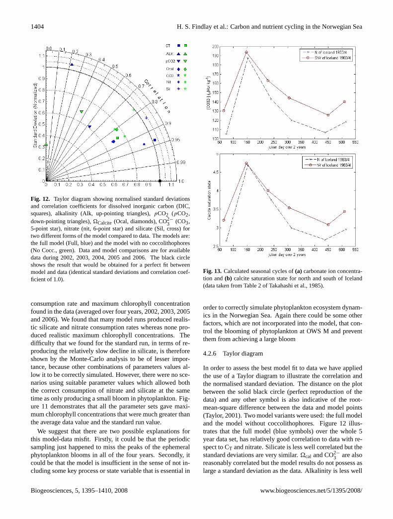
Fig. 12. Taylor diagram showing normalised standard deviationsand correlation coefficients for dissolved inorganic carbon (DIC,squares), alkalinity (Alk, up-pointing triangles),pCO2 (pCO2,down-pointing triangles),�Calcite (Ocal, diamonds), CO2−

3 (CO3,5-point star), nitrate (nit, 6-point star) and silicate (Sil, cross) fortwo different forms of the model compared to data. The models are:the full model (Full, blue) and the model with no coccolithophores(No Cocc., green). Data and model comparisons are for availabledata during 2002, 2003, 2004, 2005 and 2006. The black circleshows the result that would be obtained for a perfect fit betweenmodel and data (identical standard deviations and correlation coef-ficient of 1.0).

consumption rate and maximum chlorophyll concentrationfound in the data (averaged over four years, 2002, 2003, 2005and 2006). We found that many model runs produced realis-tic silicate and nitrate consumption rates whereas none pro-duced realistic maximum chlorophyll concentrations. Thedifficulty that we found for the standard run, in terms of re-producing the relatively slow decline in silicate, is thereforeshown by the Monte-Carlo analysis to be of lesser impor-tance, because other combinations of parameters values al-low it to be correctly simulated. However, there were no sce-narios using suitable parameter values which allowed boththe correct consumption of nitrate and silicate at the sametime as only producing a small bloom in phytoplankton. Fig-ure 11 demonstrates that all the parameter sets gave maxi-mum chlorophyll concentrations that were much greater thanthe average data value and the standard run value.

We suggest that there are two possible explanations forthis model-data misfit. Firstly, it could be that the periodicsampling just happened to miss the peaks of the ephemeralphytoplankton blooms in all of the four years. Secondly, itcould be that the model is insufficient in the sense of not in-cluding some key process or state variable that is essential in

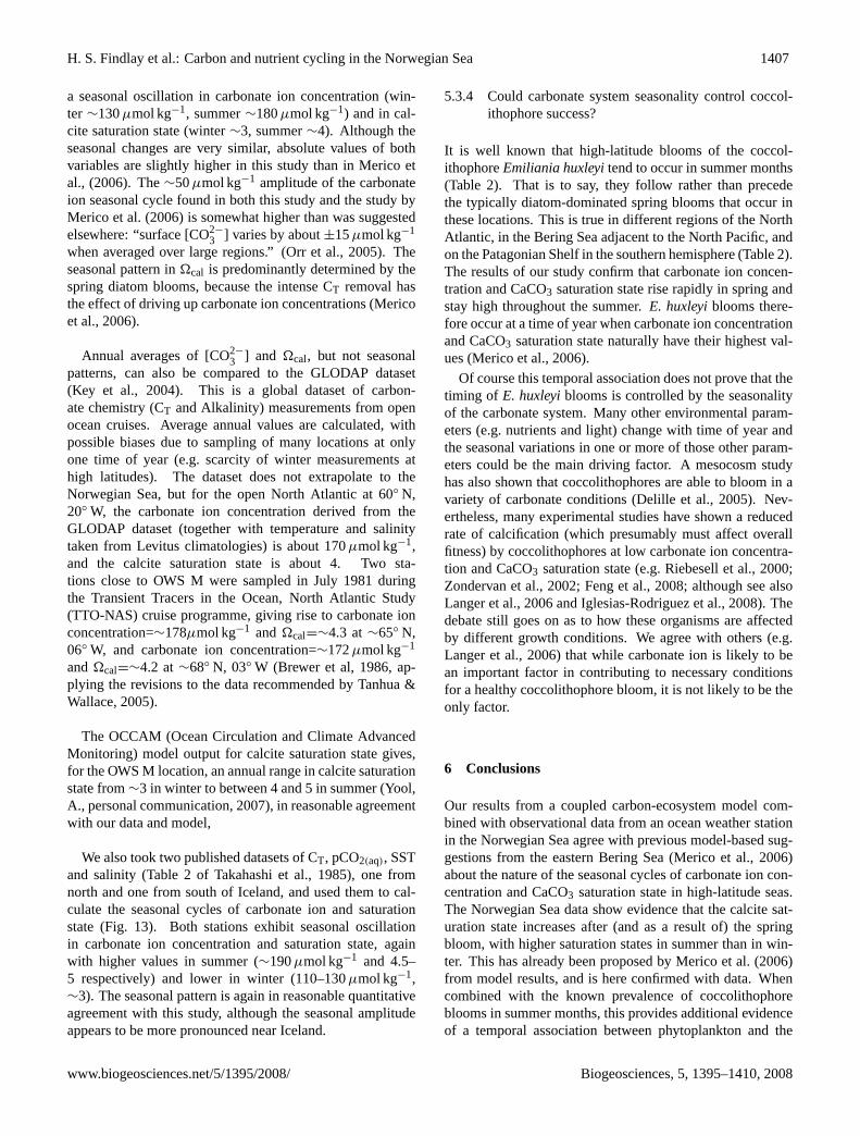
Fig. 13. Calculated seasonal cycles of(a) carbonate ion concentra-tion and(b) calcite saturation state for north and south of Iceland(data taken from Table 2 of Takahashi et al., 1985).

order to correctly simulate phytoplankton ecosystem dynam-ics in the Norwegian Sea. Again there could be some otherfactors, which are not incorporated into the model, that con-trol the blooming of phytoplankton at OWS M and preventthem from achieving a large bloom

4.2.6 Taylor diagram

In order to assess the best model fit to data we have appliedthe use of a Taylor diagram to illustrate the correlation andthe normalised standard deviation. The distance on the plotbetween the solid black circle (perfect reproduction of thedata) and any other symbol is also indicative of the root-mean-square difference between the data and model points(Taylor, 2001). Two model variants were used: the full modeland the model without coccolithophores. Figure 12 illus-trates that the full model (blue symbols) over the whole 5year data set, has relatively good correlation to data with re-spect to CT and nitrate. Silicate is less well correlated but thestandard deviations are very similar.�cal and CO2−

3 are alsoreasonably correlated but the model results do not possess aslarge a standard deviation as the data. Alkalinity is less well



correlated but shows good resemblance to the variation of thedata. When the no coccolithophore model is used (Fig. 12,green symbols), all variables become less correlated with thedata than when using the full model. All the variables exceptfor nitrate, CT and alkalinity have a slightly better represen-tation of the variation in the data; alkalinity, nitrate and CTall have lower standard deviations.

5 Discussion

5.1 The ecosystem and nutrient dynamics

In this section we compare the seasonal patterns of phyto-plankton and nutrients at OWS M to those at several otherlocations, and conclude that some factor (possibly iron lim-itation) restricts phytoplankton growth at OWS M in someyears.

5.1.1 Nitrate

Previous data suggest that in some years Norwegian Seanitrate concentrations never reach limiting levels, while inother years nitrate is fully depleted but not until later insummer (Kohly, 1998; Dale et al., 1999; Haupt et al.,1999). Neither the model nor the data shown here agreewith these previous observations. Minimum nitrate for 2002,2003, 2005 and 2006, respectively, is 0.35, 0.43, 0.52 and1.79 mmol N m−3 in the model and 0.26, 0.02, 0.18 and0.03 mmol N m−3 in the data (Fig. 4). This behaviour atOWS M (slow and/or incomplete nitrate depletion in someyears) is somewhat at odds with the more commonly ob-served pattern in temperate and sub-polar waters: that nitrateand silicate are rapidly exhausted as a consequence of in-tense spring phytoplankton blooms, and then remain scarcethroughout summer. Such a situation is seen in, for exam-ple: (1) the eastern Bering Sea (Merico et al, 2004), (2) theIrish Sea (Tyrrell et al, 2005), (3) the Baltic Sea (Larssonet al, 2001), and (4) the North Atlantic at∼(47◦ N,20◦ W)(Fasham et al., 2001; Takahashi et al., 1993), and (5) northof Iceland at about∼(68◦ N, 19◦ W) (Takahashi et al, 1993).On the other hand, residual summer nitrate has also been ob-served in the Irminger Basin between Iceland and Green-land (Henson et al., 2003; Takahashi et al., 1993), eastof Iceland at∼(64◦ N,10◦ W) (Allen et al., 2005), and at∼(60◦ N,20◦ W) in the North Atlantic (Taylor et al., 1993).

5.1.2 Silicate

The OWS M silicate data do not agree with the simulations.In the model, diatoms bloom but soon become limited byrapidly depleting silicate, which is already at a fairly lowconcentration prior to the spring blooms. This results in themonly having a relatively short bloom. The pattern in the datais very different (Fig. 8). Silicate is not rapidly consumed

in any of the four years (Fig. 4), implying that either the di-atoms are not rapidly blooming (even though silicate shouldonly become limiting to blooms at<2 mmol m−3, Egge andAksnes, 1992) or else that there is an influx of silicate whichis able to counterbalance any rapid consumption.

5.1.3 Chlorophyll

The peak springtime chlorophyll concentrations (≤3 mg chl-a m−3, Figure 4) observed at OWS M between 2002 and2006 are quite low compared to other locations in shelf seas,e.g. 16 mg chl-a m−3 in the eastern Bering Sea (Merico et al.,2004) and∼11 mg chl-a m−3 in the Irish Sea (Tyrrell et al.,2005). Similar small maximum values have however beenobserved in other (open-ocean) settings such as the LabradorSea (2–3 mg chl-a m−3, Boss et al., 2008) and the North At-lantic at∼(47◦ N, 20◦ W) (∼3 mg chl-a m−3: Fasham et al.,2001). However, the bloom chlorophyll levels observed inthe Norwegian Sea are significantly greater than typical an-nual maxima in HNLC areas which are usually≤1 mg chl-a m−3 (for instance the Subarctic Northeast and NorthwestPacific and the Southwest Bering Sea, Tyrrell et al., 2005;Boyd et al., 1998). The Monte-Carlo parameter analysis sug-gests that out of 200 model runs, with parameter values allo-cated randomly within ranges determined from the literature,it was not possible to create the small chlorophyll maximumseen in the data, yet the model appears to have a good corre-lation to the data in terms of CT and nitrate annual cycles.

5.1.4 Interpretation

The slow and/or incomplete exhaustion rates of nitrate and,especially, silicate, at OWS M are atypical compared to someother locations. Various hypotheses have been proposedto explain this phenomenon including grazer levels (Tayloret al., 1993, as an explanation for residual summer nitrateat 60◦ N, 20◦ W in the North Atlantic) and silicate-limitedgrowth of diatoms (Dale et al., 1999).

Analyses of longer term datasets for this area agree thatthere are low chlorophyll levels during the spring bloom andthere is slow silicate consumption, although there is morevariability over longer time periods (Rey, personal commu-nication, 2007). They suggest that the preferential grazing ofzooplankton on diatoms may explain the relatively slow de-pletion of silicate. However, the selective grazing function inour model does not prevent the rapid blooming of diatomsin the spring, thus neither reproducing the observed lowchlorophyll levels nor a slow silicate drawdown; studies haveshown that the dominant zooplankton grazers in the Norwe-gian Sea,Calanus helgolandicusandCalanus finmarchicus(Gaard, 2000) both have reduced reproductive output duringdiatom dominated blooms and hence preferentially graze onnon-diatom species (Nejstgaard et al., 2001).

The data from OWS M clearly show that it is not a fullHigh Nutrient Low Chlorophyll (HNLC) area, as, although



peak chlorophyll concentrations are low, they are not as lowas in true HNLC areas and nutrient concentrations do fluc-tuate considerably across the seasonal cycle. Previous worksuggests that phytoplankton growth in spring in the NorthAtlantic is influenced by levels of iron (Moore et al., 2006).This raises the question as to whether spring blooms at OWSM could also be restrained by low levels of iron in someyears. OWS M lies on the continental slope and is subjectto different conditions to shelf seas, but is also not an openocean system. One possible explanation of the low chloro-phyll levels and slow/incomplete nutrient depletion in someyears could be that iron scarcity inhibits large phytoplanktonblooms during some years but not others. The interannualvariability could thus potentially be explained by the advec-tion of coastal waters across OWS M only in some years(this often occurs around August time, as determined fromsea surface salinity measurements). Coastal and shelf waterstypically have higher iron content due to iron release fromsediments (e.g. Aguilar-Islas et al., 2007).

5.2 Local CO2 sink strengths

The annual cycle of carbon dioxide partial pressure in thesurface waters (pCO2(SW)) has been explored here. At thestart of the year pCO2(SW) decreases as a result of the colderwater temperatures and the continued vertical exchange ofcarbon that carries on until the summer pycnocline hasformed. The spring bloom rapidly consumes CO2 from thesurface water and hence decreases the partial pressure, (byup to 100µ atm) (Fig. 5). The removal of pCO2(SW) occursthroughout the summer until the breakdown of stratificationand the end of biological production.

For the first part of the year until the end of the biolog-ical production period, the waters act as a sink for carbondioxide, with an average model CO2 flux of 37 g C m−2 yr−1

from the atmosphere to the surface water. Falck and Ander-son (2005) calculated a flux of CO2 of 32 g C m−2 yr−1 forOWS M data during 1991–1994 and Skjelvan et al. (2005)suggest 20 g C m−2 yr−1 for the Norwegian Sea. Otherestimates for the Nordic Seas area include a flux of53 g C m−2 yr−1 into the Greenland Sea (Anderson et al.,2000) and 69 g C m−2 yr−1 into the Iceland Sea (Skjelvan etal., 1999). The variability in fluxes between locations in theNordic Seas may result from the varying amounts of primaryproduction, the varying hydrographic conditions and/or thedifferent water masses occurring at each location.

5.3 Comparison to other carbonate system measurementsin waters with abundant coccolithophores

5.3.1 Alkalinity

Robertson et al. (1994), in the North Atlantic, south of Ice-land, gives AT values within areas that do not have coccol-ithophores present of about 2330µEq kg−1 (comparable to

the modelled winter values in the Norwegian Sea: 2320µ

Eq kg−1). Areas where coccolithophore blooms had oc-curred, gave lower AT values (lowest AT<2290µ Eq kg−1

at approximately 63◦ N, 22◦ W). This implies that areas har-bouring intense coccolithophore blooms can experience re-ductions in AT of about 50–60µ Eq kg−1. These decreaseswere not due to either nitrate or salinity effects on alkalinitybecause differences in the two parameters were small in thestudy area (Holligan et al., 1993a). We can assume that about20µ Eq kg−1 of the alkalinity change is due to salinity reduc-tions (Skjelvan et al., 2008); however there remains a contri-bution by calcification of about 30µ Eq kg−1. Satellite dataconfirm this view: SeaWiFS derived calcite concentrationsfor the OWS M location range from about 0.5 mmol CaCO3-C m−3 in winter to a maximum of 4 mmol CaCO3-C m−3 insummer in some years (SeaWiFS Project, 2006). These val-ues are in agreement with values of modelled calcite, pro-duced as free coccoliths (range from 0 mmol C m−3 to 3.5mmol C m−3). Interestingly, SeaWiFS images show that coc-colithophore blooms commonly occur along the Norwegiancoast but sometimes also extend out as far as the shelf breakwhere OWS M is situated (SeaWiFS Project, 2006).

5.3.2 Dissolved inorganic carbon

CT concentration in the Norwegian Sea in winter wasabout 2140µmol kg−1, while in June–July it was about2080µmol kg−1, which is a similar value to non-coccolithophore bloom areas in July 1991 in the North At-lantic (Robertson et al., 1994). The lowest CT concentrationreached in the Norwegian Sea was about 2050µmol kg−1,again similar to values measured south of Iceland. Takahashiet al. (1993) show that in the northeastern North Atlantic CTdeclined by about 60µmol kg−1 during the phytoplanktonbloom period in late March through to late May (during theNorth Atlantic Bloom Experiment study in 1989).

5.3.3 Carbonate ion and calcite saturation state

Merico et al. (2006) modelled the seasonal cycle of car-bonate chemistry in the eastern Bering Sea (specific lo-cation: 56.8◦ N, 164◦ W). The model calculated consid-erable seasonal variation in both carbonate ion (winter∼100µmol kg−1, summer∼150µmol kg−1) and calcite sat-uration state (winter∼2.5, summer∼3.5). Both variableswere low in winter, rose sharply at the time of the springblooms, and then stayed high during the summer until de-clining in autumn due to mixing. There was, however, a lackof data with which to test these model results in the east-ern Bering Sea. In contrast, data are available for modelcomparison in this study. Our results from the NorwegianSea shelf break (Ocean Weather Station M, 66◦ N, 2◦ E)agree in outline with the model predictions for the east-ern Bering Sea (compare Fig. 5 in Merico et al., 2006 andFig. 6 of this paper). The Norwegian Sea data also show



a seasonal oscillation in carbonate ion concentration (win-ter ∼130µmol kg−1, summer∼180µmol kg−1) and in cal-cite saturation state (winter∼3, summer∼4). Although theseasonal changes are very similar, absolute values of bothvariables are slightly higher in this study than in Merico etal., (2006). The∼50µmol kg−1 amplitude of the carbonateion seasonal cycle found in both this study and the study byMerico et al. (2006) is somewhat higher than was suggestedelsewhere: “surface [CO2−

3 ] varies by about±15µmol kg−1

when averaged over large regions.” (Orr et al., 2005). Theseasonal pattern in�cal is predominantly determined by thespring diatom blooms, because the intense CT removal hasthe effect of driving up carbonate ion concentrations (Mericoet al., 2006).

Annual averages of [CO2−

3 ] and �cal, but not seasonalpatterns, can also be compared to the GLODAP dataset(Key et al., 2004). This is a global dataset of carbon-ate chemistry (CT and Alkalinity) measurements from openocean cruises. Average annual values are calculated, withpossible biases due to sampling of many locations at onlyone time of year (e.g. scarcity of winter measurements athigh latitudes). The dataset does not extrapolate to theNorwegian Sea, but for the open North Atlantic at 60◦ N,20◦ W, the carbonate ion concentration derived from theGLODAP dataset (together with temperature and salinitytaken from Levitus climatologies) is about 170µmol kg−1,and the calcite saturation state is about 4. Two sta-tions close to OWS M were sampled in July 1981 duringthe Transient Tracers in the Ocean, North Atlantic Study(TTO-NAS) cruise programme, giving rise to carbonate ionconcentration=∼178µmol kg−1 and�cal=∼4.3 at∼65◦ N,06◦ W, and carbonate ion concentration=∼172µmol kg−1

and�cal=∼4.2 at∼68◦ N, 03◦ W (Brewer et al, 1986, ap-plying the revisions to the data recommended by Tanhua &Wallace, 2005).

The OCCAM (Ocean Circulation and Climate AdvancedMonitoring) model output for calcite saturation state gives,for the OWS M location, an annual range in calcite saturationstate from∼3 in winter to between 4 and 5 in summer (Yool,A., personal communication, 2007), in reasonable agreementwith our data and model,

We also took two published datasets of CT, pCO2(aq), SSTand salinity (Table 2 of Takahashi et al., 1985), one fromnorth and one from south of Iceland, and used them to cal-culate the seasonal cycles of carbonate ion and saturationstate (Fig. 13). Both stations exhibit seasonal oscillationin carbonate ion concentration and saturation state, againwith higher values in summer (∼190µmol kg−1 and 4.5–5 respectively) and lower in winter (110–130µmol kg−1,∼3). The seasonal pattern is again in reasonable quantitativeagreement with this study, although the seasonal amplitudeappears to be more pronounced near Iceland.

5.3.4 Could carbonate system seasonality control coccol-ithophore success?

It is well known that high-latitude blooms of the coccol-ithophoreEmiliania huxleyitend to occur in summer months(Table 2). That is to say, they follow rather than precedethe typically diatom-dominated spring blooms that occur inthese locations. This is true in different regions of the NorthAtlantic, in the Bering Sea adjacent to the North Pacific, andon the Patagonian Shelf in the southern hemisphere (Table 2).The results of our study confirm that carbonate ion concen-tration and CaCO3 saturation state rise rapidly in spring andstay high throughout the summer.E. huxleyiblooms there-fore occur at a time of year when carbonate ion concentrationand CaCO3 saturation state naturally have their highest val-ues (Merico et al., 2006).

Of course this temporal association does not prove that thetiming of E. huxleyiblooms is controlled by the seasonalityof the carbonate system. Many other environmental param-eters (e.g. nutrients and light) change with time of year andthe seasonal variations in one or more of those other param-eters could be the main driving factor. A mesocosm studyhas also shown that coccolithophores are able to bloom in avariety of carbonate conditions (Delille et al., 2005). Nev-ertheless, many experimental studies have shown a reducedrate of calcification (which presumably must affect overallfitness) by coccolithophores at low carbonate ion concentra-tion and CaCO3 saturation state (e.g. Riebesell et al., 2000;Zondervan et al., 2002; Feng et al., 2008; although see alsoLanger et al., 2006 and Iglesias-Rodriguez et al., 2008). Thedebate still goes on as to how these organisms are affectedby different growth conditions. We agree with others (e.g.Langer et al., 2006) that while carbonate ion is likely to bean important factor in contributing to necessary conditionsfor a healthy coccolithophore bloom, it is not likely to be theonly factor.

6 Conclusions

Our results from a coupled carbon-ecosystem model com-bined with observational data from an ocean weather stationin the Norwegian Sea agree with previous model-based sug-gestions from the eastern Bering Sea (Merico et al., 2006)about the nature of the seasonal cycles of carbonate ion con-centration and CaCO3 saturation state in high-latitude seas.The Norwegian Sea data show evidence that the calcite sat-uration state increases after (and as a result of) the springbloom, with higher saturation states in summer than in win-ter. This has already been proposed by Merico et al. (2006)from model results, and is here confirmed with data. Whencombined with the known prevalence of coccolithophoreblooms in summer months, this provides additional evidenceof a temporal association between phytoplankton and the



carbonate system, which could possibly occur because coc-colithophore success is related to the calcite saturation state.

Unlike the model, the data show that silicate is not rapidlyexhausted by diatoms during the spring bloom, in contrastto the typical dynamics elsewhere; the data also highlightthe possibility that grazing and macro-nutrient dynamics arenot alone in controlling the observed nutrient and chlorophyllconcentrations at OWS M, suggesting that there may be par-tial iron limitation. This is in agreement with recent work re-vealing that other ocean regions, such as the North Atlantic,are influenced by iron availability (Moore et al., 2006).

Acknowledgements.HF acknowledges funding from a NERCMasters studentship. This work was partly funded by the Geo-physical Institute (University of Bergen), the Bjerknes Centrefor Climate Research, the European Commission through the 6thFramework Programme (EU FP6 CARBOOCEAN IP, Contractno. 511176), and the Norwegian Research Council through theCABANERA (project number: 155936/700). The authors wouldalso like to thank A. Yool for OCCAM model comparisons and F.Rey for comments on the nutrient and chlorophyll dynamics.

Edited by: U. Riebesell

References

Aguilar-Islas, A. M., Hurst, M. P., Buck, K. N., Sohst, B., Smith, G.J., Lohan, M. C., and Bruland, K. W.: Micro- and macronutrientsin the southeastern Bering Sea: Insight into iron-replete and iron-depleted regimes, Prog. in Ocean., 73, 99–126, 2007.

Allen, J. T., Brown, L., Sanders, R., et al.: Diatom carbon exportenhanced by silicate upwelling in the northeast Atlantic, Nature,437, 728–732, 2005.

Anderson, L. A. and Sarmiento, J. L.: Redfield ratios of rem-ineraliszation determined by nutrient data-analysis, Global Bio-geochem. Cy., 8, 65–80, 1994.

Anderson, L. G., Drange, H., Chierici, M., Fransson, A., Johan-nessen, T., Skjelvan, I., and Rey, F.: Annual carbon fluxes in theupper Greenland Sea based on measurements and a box-modelapproach, Tellus, 52B, 1013–1024, 2000.

Anderson, T. R.: Plankton functional type modelling: running be-fore we can walk? J. Plankton Res., 27, 1073–1081, 2005.

Andruleit, H.: Coccolithophore fluxes in the Norwegian-GreenlandSea: seasonality and assemblage alterations, Mar. Micropaleo.,31, 45–64, 1997.

Andruleit, H.: Dissolution-affected coccolithophore fluxes in thecentral Greenland Sea (1994/1995), Deep-Sea Res. II, 47, 1719–1742, 2000.

Baumann, K.-H., Andruleit, H. A., and Samtleben, C.: Coccol-ithophores in the Nordic Seas: comparison of living communitieswith surface sediment assemblages, Deep-Sea Res. II, 47, 1743–1772, 2000.

Bellerby, R. G. J., Olsen, A., Furevik, T., and Anderson, L. G.: Re-sponse of the surface ocean CO2 system in the Nordic Seas andNorthern North Atlantic to Climate Change, Geophys. Mono.Ser., 158, 189–198, 2005.

Boss, E., Perry, M. J., Swift, D., Taylor, L., Brickely, P., Zaneveld, J.R. V., and Riser, S.: Three years of ocean data from a bio-opticalprofiling float, EOS, Transactions of the American GeophysicalUnion, 89, 209–210, 2008.

Boyd, P. B., Wong, C. S., Merrill, J., Whitney, F,. Snow, J., Harri-son, P. J., and Gower, J.: Atmospheric iron supply and enhancedvertical carbon flux in the NE subarctic Pacific: Is there a con-nection?, Global Biogeochem. Cy., 12, 429–441, 1998.

Brewer, P. G., Takahashi, T., and William, R. T.: Transient Trac-ers in the Oceans (TTO) – Hydrographic data and carbon diox-ide systems with revised carbon chemistry data, NDP-004/R1,Carbon Dioxide Information Center, Oak Ridge National Labo-ratory, Oak Ridge, Tennessee, 1986.

Brostrom, G.: A note on the C/N and C/P ratio of the biologicalproduction in the Nordic Seas, Tellus, 50B, 93–109, 1998.

Brown, C. W. and Yoder, J. A.: Coccolithophorid blooms in theglobal ocean. J. Geophys. Res., 99, 7467–7482, 1994a.

Brown, C. W. and Yoder, J. A.: Distribution patterns of coccol-ithophorid blooms in the western North Atlantic Ocean, Cont.Shelf. Res., 14, 175–197, 1994b.

Burkhill, P. H., Leakey, R. J. G., Owens, N. J. P., and Mantoura R. F.C.: Synechococcus and its imortnace to the microbial foodweb ofthe northwestern Indian Ocean, Deep-Sea Res. II, 40, 773–382,1993.

Calbet, A. and Landry, M. R.: Phytoplankton growth, microzoo-plankton grazing, and carbon cycling in marine systems, Limn.and Ocean., 49, 51–57, 2004.

Cloern, J. E., Grenz, C., and Vidergar-Lucas, L.: An empiricalmodel of phytoplankton chlorophyll: carbon ratio – the con-version factor between productivity and growth rate, Lim. andOcean., 40, 1313–1321, 1995.

Dale, T., Rey, F., and Heimdal, B.R.: Seasonal developments ofphytoplankton at a high latitude oceanic site, Sarsia, 84, 419-435, 1999.

Dale, T., Kaartvedt, S., Ellertsen, B., and Amundsen, R.: Large-scale oceanic distribution and population structure of Calanusfinmarchicus in relation to physical food and predators, Mar.Bio., 139, 561–574, 2001.

Delille, B. Harley, J., Zondervan, I., Jacquet, S., Chou, L., Wollast,R., Bellerby, R. G. J., Frankignoulle, M., Borges, A. V., Riebe-sell, U., and Gattuso, J.-P.: Response of primary production andcalcification to changes ofpCO2 during experimental blooms ofthe coccolithophorid Emiliania huxleyi, Gobal Biogeochem. Cy-cles, 19, GB2023, doi:10.1029/2004GB002318, 2005

Egge, J. K. and Aksnes, D. L.: Silicate as regulating nutrient inphytoplankton competition, MEPS, 83, 281–289, 1992.

Eppley, R. W.: Temperature and phytoplankton growth in the sea,Fishery Bull., 70, 1063–1085, 1972.

Evans, G. T., and Parslow, J. S.: A model of annual plankton cycles,Bio. Ocean., 3, 327–247, 1985.

Falck, E. and Anderson, L. G.: The dynamics of the carbon cycle inthe surface water of the Norwegian Sea, Mar. Chem., 94, 43–53,2005.

Fasham, M. J. R., Ducklow, H. W., and McKelvie, S. M.: Anitrogen-based model of plankton dynamics in the oceanic mixedlayer, J. Mar. Res., 48, 591–639, 1990.

Fasham, M. J. R.: Modelling marine biota, in: The Global Car-bon Cycle, edited by: Heimann, M., Springer-Verlag, Heidel-berg, 457–504, 1993.



Fasham, M. J. R., Balino, B. M., and Bowles, M. C.: Joint OceanGlobal Flux Study (JGOFS), AMBIO, Special Report, 10, 4–31,2001.

Feng, Y., Warner, M. E., Zhang, Y., Sun, J., Fu, F. X., Rose, J. M.,and Hutchins, D. A.: Interactive effects of increasedpCO2, tem-perature and irradiance on the marine coccolithophoreEmilianiahuxleyi(Prymnesiophyceae), Eur. J. Phycol., 43, 87–98, 2008.

Friis, K., Kortzinger A., and Wallace, D.W.R.: The salinity nor-malization of marine inorganic carbon chemistry data, Geophys.Res. Lett., 20, 1085, doi:10.1029/2002GL015898, 2003.

Gaard, E.: Seasonal abundance and development of Calanus fin-marchicus in relation to phytoplankton and hydrography on theFaroe Shelf, ICES J. Mar. Sci., 57, 1605–1611, 2000.

Garcon, V. C., Thomas, F., Wong, C. S., and Minster, J.-F.: Gaininginsight into the seasonal variability of CO2 at Ocean Station Pusing an upper ocean model, Deep-Sea Res., 39, 921–938, 1992.

Gislefoss, J. S., Nydal, R., Slagstad, D., Sonninen, E., and Holme,K.: Carbon time series in the Norwegian Sea, Deep-Sea Res. I,45, 433–460, 1998.

Halvorsen, E., Tande, K. S., Edvardsen, A., Slagstad, D., and Peder-sen, O. P.: Habitat selection of overwintering Calanus finmarchi-cus in the NE Norwegian Sea and shelf waters of Northern Nor-way in 2000–2002, Fisheries Ocean., 12, 339–351, 2003.

Haupt, O. J., Wolf, U., and Von Bodungen, B.: Modelling thepelagic nitrogen cycle and vertical particle flux in the NorwegianSea, J. Mar. Sys., 19, 173–199, 1999.

Henson, S. A., Sanders, R., Allen, J. T. Robinson, I. S., andBrown, L.: Seasonal constraints on the estimation of new pro-duction from space using temperature-nitrate relationships, Geo-phys. Res. Lett., 30, 1912, doi:10.1029/2003GL017982, 2003.

Holligan, P. M., Fernandez, E., Aiken, J., Balch, W. M., Boyd, P.,Burkhill, P. H., Finch, M., Groom, S. B., Malin, G., Muller, K.,Purdie, D. A., Robinson, C., Trees, C. C., Turner, S. M., andVan der Wal, P.: A biogeochemical study of coccolithophore,Emiliania huxleyi, in the North Atlantic, Glob. Biogeochem. Cy.,7, 879–900, 1993a.

Holligan, P. M., Groom, S. B., and Harbour, D. S.: What controlsthe distribution of the coccolithophore,Emiliania huxleyi, in theNorth Sea?, Fisheries Oceanog., 2, 175–183, 1993b.

Kahler, P. and Koeve, W.: Marine dissolved organis matter: canits C:N ratio explain carbon overconsumption?, Deep-Sea Res. I,48, 49–62, 2001.

Key, R. M., Kozyr, A., Sabine, C. L., Wanninkhof, R., Bullis-ter, J. L., Feely, R. A., Millero, F. J., Mordy, C., and Peng, T.H.: A global ocean carbon climatology: Results from GlobalData Analysis Project (GLODAP), Global Biogeochem. Cy., 18,GB4031, 2004.

Kohly, A.: Diatom flux and species composition in the GreenlandSea and the Norwegian Sea in 1991–1992, Mar. Geol., 145, 293–312, 1998.

Kortzinger, A., Koeve, W., Kahler, P., and Mintrop, L.: C:N ratiosin the mixed layer during the productive season in the northeastAtlantic Ocean, Deep-Sea Res. I, 48, 661–688, 2001.

Langer, H., Geisen, M., Baumann, K.-H., Klas, J., Riebe-sell, U., Thoms, S., and Yonge, J. R.: Species-specific re-sponseses of calcifying alga to changing seawater carbon-ate chemistry, Geochem. Geophys. Geosys., 7, Q09006, doi:10.1029/2005GC001227, 2006.

Larsson, U., Hajdu, S., Walve, J., and Elmgren, R.: Baltic Sea nitro-gen fixation estimated from the summer increase in upper mixedlayer total nitrogen, Limnol. Oceanogr., 46, 811–820, 2001.

Merico, A., Tyrrell, T., Lessard, E. J., Oguz, T., Stabeno, P. J., Zee-man, S. I., and Whitledge, T. E.: Modelling phytoplankton su-cession on the Bering Sea shelf: role of climate influences andtrophic interactions in generating Emiliania huxleyi blooms in1997–2000, Deep-Sea Res. I, 51, 1803–1826, 2004.

Merico, A., Tyrrell, T., and Cokacar, T.: Is there any relationship be-tween phytoplankton seasonal dynamics and the carbonate sys-tem?, J. Mar. Sys., 59(1–2), 120–142, 2006.

Miller, L.A., Chierici, M., Johannessen, T., Noji, T.T., Rey, F., andSkjelvan, I.: Seasonal dissolved inorganic carbon variations inthe Greenland Sea and implications for atmospheric CO2 ex-change, Deep-Sea Res. II, 46, 1472–1496, 1999.

Millero, F. J., Lee, K., and Roche, M.: Distribution of alkalinity inthe surface waters of the major oceans, Mar. Chem., 45, 111–130,1998.

Moore, C. M., Mills, M. M., Milne, A., Langlois, R., Achterberg,E. P., Lochte, K., Eider, R. J. G., and La Roche, J.: Iron lim-its primary productivity during spring bloom development in thecentral North Atlantic, Glob. Change Bio., 12, 626–634, 2006.

Murata, A.: Increased surface waterpCO2 in the eastern BeringSea shelf: An effect of blooms of coccolithophorid Emilianiahuxleyi?, Global Biogeochem. Cy., 20, GB4006, 1–9, 2006.

Najjar, R. G.: Marine Biogeochemistry, in: Climate System Mod-elling, edited by: Trenberth, K. E., Cambridge University Press,Cambridge, 241–280, 1992.

Nejstgaard, J. C., Hygum, B. H., Naustvoll, L. J., and Bamstedt,U.: Zooplankton growth, diet and reproductive success com-pared in simultaneous diatom- and flagellate-microzooplankton-dominated plankton blooms, Mar. Ecol. Prog. Ser., 221, 77–91,2001.

Nilsen, J. E. O. and Falck, E.: Variations in mixed layer propertiesin the Norwegian Sea for the period 1948–1999, Prog. in Ocean.,70, 58–90, 2006.

Nondal, G., Bellerby, R. G. J., Olsen, A., Johannessen, T., and Olaf-sson, J.: Predicting the surface ocean CO2 system in the northernNorth Atlantic: Implications for the use of Voluntary ObservingShips, Limnol. Oceanogr.. submitted, 2008.

Oliver, K. I. C. and Heywood, K. J.: Head and freshwater fluxesthrough the Nordic Seas, J. Phys. Ocean., 33, 1009–1026, 2003.

Orvik, K. A. and Skagseth, O.: The impact of the wind stress curl inthe North Atlantic on the Atlantic inflow to the Norwegian Seatoward the Arctic, Geophys. Res. Lett., 30(17), p. 1884, 2003.

Orr, J. C., Fabry, V. J., Aumont, O., et al.: Anthropogenic oceanacidification over the twenty-first century and its impact on cal-cifying organisms, Nature, 437, 681–686, 2005.

Peng, T. H., Takahashi, T., Broecker, W. S., and Olafsson, J.: Sea-sonal variability of carbon dioxide, nutrients and oxygen in thenorthern North Atlantic surface water: observations and a model,Tellus, 39B, 439–458, 1987.

Peinert, R., Bodungen, B. V., and Smetacek, V. S.: Food web struc-ture and loss rate, in: Productivity of the Ocean: Present andPast, edited by: Berger, W. H., Smetacek, V. S., and Wefer, G.,John Wiley & Sons Limited, 35–48, 1989.



Raitsos, D. E., Lavender, S. J., Pradhan, Y., Tyrrell, T., Reid, P.C., and Edwards, M.: Coccolithophore bloom size variation inresponse to the regional environment of the subarctic North At-lantic. Limnol. Oceanogr., 51, 2122–2130, 2006.

Redfield, A. C., Ketchum, B. H., and Richards, F. A.: The influenceof organisms on the composition of seawater, in: The Sea, editedby: Hill, M. N., Wiley, New York, 26–77, 1963.

Riebesell, U., Zondervan, I., Rost, B., Tortell, P. D., Zeebe, R. E.,and Morel, F. M. M.: Reduced calcification of marine planktonin response to increase atmospheric CO2, Nature, 407, 634–637,2000.

Robertson, J. E., Robinson, C., Turner, D. R., Holligan, P., Watson,A. J., Boyd, P., Fernandez, E., and Finch, M.: The impact of acoccolithophore bloom on oceanic carbon uptake in the northeastAtlantic during summer 1991, Deep-Sea Res. I, 41, 279–314,1994.

Sambrotto, R. N., Savidge, G., Robinson, C., Boyd, P., Takahashi,T., Karl, D. M., Langdon, C., Chipman, D., Marra, J., andCopdispoti, L.: Elevated consumption of carbon relative to ni-trogen in the surface ocean, Nature, 363, 248–250, 1993.

Skjelvan, I., Chierici, M., and Olafsson, J.: Horizontal distributionsof NCT, NAT and fCO2 in the Nordic Seas, In Carbon and Oxy-gen Fluxes, in: the Nordic Seas, Skjelvan, I., PhD thesis, Univer-sity of Bergen, Norway, 1999.

Skjelvan, I., Olsen, A., Anderson, L. G., Bellerby, R. G. J., Falck,E., Kasajima, Y., Kivimae, C., Omar, A., Rey, F., Olsson, A., Jo-hannessen, T., and Heinze, C.: A review of the inorganic carboncycle of the Nordic Seas and Barents Sea, Geophys. Mono., 158,157–176, 2005.

Skjelvan, I., Falck, E., Rey, F., and Kringstad, S. B.: Inorganic car-bon time series at Ocean Weather Station M in the NorwegianSea, Biogeosciences, 5, 549–560, 2008,http://www.biogeosciences.net/5/549/2008/.

Smyth, T. J., Tyrrell, T., and Tarrant, B.: Time se-ries of coccolithophore activity in the Barents Sea, fromtwenty years of satellite imagery, Geophys. Res. Lett., 31,doi:10.1029/2004GL019735, 2004.

Takahashi, T.,Olafsson, J., Broecker, W. S., Goddard, J., Chip-man, D. W., and White, J.: Seasonal variability of the carbon-nutrient chemistry in the ocean areas west and north of Iceland,Rit Fiskideildar, 9, 20–36, 1985.

Takahashi, T.,Olafsson, J., Goddard, J. G., Chipman, D. W., andSutherland, S. C.: Seasonal variability of CO2 and nutrients inthe high-latitude surface oceans: a comparative study, Glob. Bio-geochem. Cy., 7, 843–878, 1993.

Tanhua, T. and Wallace D. W. R.: Consistency of TTO-NAS Inor-ganic Carbon Data with modern measurements, Geophys. Res.Lett., 32, L14618, doi:10.1029/2005G:032348, 2005.

Taylor, A. H., Harbour, D. S., Harris, R. P., Burkhill, P. H., andEdwards, E. S.: Seasonal succession in the pelagic ecosystem ofthe North Atlantic and the utilization of nitrogen, J. Plank. Res.,15, 875–891, 1993.

Taylor, K. E.: Summarizing multiple aspects of model performancein a single diagram, J. Geophys. Res.-Atmos., 106 (D7), 7183–7192, 2001.

Tyrrell, T., Hollligan, P. M., and Mobley, C. D.: Optical impactsof oceanic coccolithophore blooms, J. Geophys. Res.-Oceans,104(C2), 3223–3241, 1999.

Tyrrell, T. and Merico, A.: Emiliania huxleyi: bloom observationsand the conditions that induce them, in: Coccolithophores, FromMolecular Processes to Global Impact, edited by: Thierstein, H.R. and Young, J. R., Springer, Berlin, 75–97, 2004.

Tyrrell, T., Merico, A., Waniek, J., Wong, C. S., Metzl, N., andWhitney, F.: Effect of seafloor depth on phytoplankton blooms inhigh-nitrate, low-chlorophyll (HNLC) regions, J. Geophys. Res.-Biogeosci., 110, G02007, 2005.

Zondervan, I., Rost, B., and Riebesell, U.: Effect of CO2 con-centration on the PIC/POC ratio in the coccolithophoreEmilia-nia huxleyigrown under light-limiting conditions and differentdaylengths, J. Exp. Mar. Biol. Ecol., 272, 55–70, 2002.


http://www.biogeosciences.net/5/549/2008/

biogeosciences carbon and nutrient mixed layer dynamics in the

Documents