BIOETHANOL POTENTIAL OF

PRESERVED BIOWASTE

Magdalena Gerlach

Bachelor’s thesis

May 2012

Degree Programme in Environmental

Engineering

ABSTRACT

Tampereen Ammattikorkeakoulu

Tampere University of Applied Sciences

Environmental Engineering

MAGDALENA GERLACH:

Bioethanol Potential of Preserved Biowaste

Bachelor's thesis 40 pages, appendices 17 pages

May 2012

The development of alternatives to fossil fuels like oil and natural gas is becoming

increasingly urgent with the depletion of resources of fossil fuels and the steadily

worsening state of our atmosphere and natural environment. The usage of biofuels is

one possibility to decrease greenhouse gas emissions in the nearer future, while other

environmentally friendly vehicle technologies are still under development. Bioethanol

can be used in fuels for vehicles without any modifications of the engines in

concentrations up to 5 per cent, and even 10 per cent in newer engines. Different

possible raw materials for the production of bioethanol have been studied during the last

few decades.

The handling of waste produced by human society is becoming more and more difficult

due to a growing world population and an increase in living standards world-wide. The

aim of this study is to show the bioethanol production potential of preserved food waste

in an institution like Tampere University of Applied Sciences. It investigates if the

biowaste from the TAMK kitchen, after being stored over longer time periods, is

suitable for bioethanol production.

The change in bioethanol yield was studied over a time period of three months, during

which the food residues were preserved and stored in anaerobic conditions. The

bioethanol yield, as well as other factors such as chloride content, pH, conductivity, and

dry matter content, and their fluctuation over time were analyzed over the whole three

month period.

The study showed that even though factors like chloride content, pH and conductivity

were kept at desirable levels, the bioethanol yield itself fluctuated a lot during the 3

month period. The method of adding the biowaste to the vessel - in terms of amounts

and adding rhythm - seems to have an effect on the ethanol yield. An assumption of

early fermentation taking place was not confirmed. The dry matter content could not be

analyzed accurately enough with the used method and needs to be studied further in the

future. For future projects, it would also be necessary to find out the glucose content of

the raw material to make the results more comparable to already existing studies.

Key words: Bioethanol yield, biowaste, hydrolysis, fermentation

3

CONTENTS

1 GLOSSARY ................................................................................................................ 4

2 INTRODUCTION ....................................................................................................... 5

3 BIOETHANOL ........................................................................................................... 8

3.1. Bioethanol as an alternative fuel in the past, nowadays and in the future ........... 9

3.2. Application, restrictions and advantages of bioethanol fuel .............................. 11

3.3. Sources of bioethanol ......................................................................................... 12

3.3.1 Food crops ............................................................................................... 12

3.3.2 Common crops and lignocellulosic materials ......................................... 12

3.3.3 Municipal waste ...................................................................................... 13

3.4. Production of bioethanol .................................................................................... 14

4 EXPERIMENTAL STUDIES ................................................................................... 16

4.1. Implementation of the experiment ..................................................................... 16

4.2. Analytical methods ............................................................................................ 19

4.2.1 Bioethanol potential ................................................................................ 19

4.2.2 Chloride content ...................................................................................... 22

5 RESULTS AND CONCLUSIONS ........................................................................... 23

5.1. Presentation of the measurements ...................................................................... 23

5.1.1 pH of the preserved biowaste ................................................................. 23

5.1.2 Conductivity of the preserved biowaste .................................................. 24

5.1.3 Gas composition inside the vessel .......................................................... 24

5.1.4 Chloride content of the preserved biowaste ............................................ 25

5.1.5 Dry matter content of the preserved biowaste......................................... 26

5.1.6 Ethanol yield ........................................................................................... 28

5.2. Conclusions on the ethanol yield results ............................................................ 31

6 DISCUSSION ........................................................................................................... 36

REFERENCES ................................................................................................................ 39

APPENDICES ................................................................................................................ 41

Appendix 1. MATERIAL SAFETY DATA SHEET Formic Acid ........................... 41

Appendix 2. Biowaste materials added to the Jäte-Aate vessel over the testing

period ................................................................................................................. 44

Appendix 3. Measurements taken during the testing period (pH, conductivity,

CH4, CO2, O2) .................................................................................................. 45

Appendix 4. Chloride content analysis results of the sample from 24.11.2011 ........ 46

Appendix 5. Chloride content analysis results of the sample from 28.12.2012 ........ 49

Appendix 6. Chloride content analysis results of the sample from 18.1.2012 .......... 52

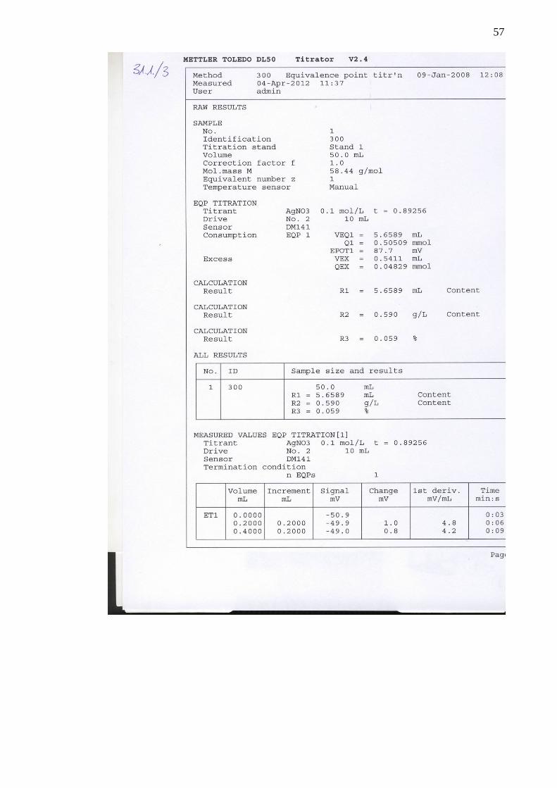
Appendix 7. Chloride content analysis results of the sample from 31.1.2012 .......... 55

4

1 GLOSSARY

Cl Chloride

CO2 Carbon dioxide

C5 Xylose-sugars

C6 Glucose-sugars

EU European Union

EtOH Ethanol

EPA US Environmental Protection Agency

MSW Municipal Solid Waste

NaCl Sodium chloride

NaOH Sodium hydroxide

NTNU Norwegian University

RDF Refuse Derived Fuel

RFA Renewable Fuels Association

RFA Renewable Fuels Association

rpm revolutions per minute

TAMK Tampere University of Applied Sciences

5

2 INTRODUCTION

While the world is running short on fossil fuels in the near future, the production of

solid waste and biowaste is growing steadily at the same time due to a growing world

population and a rising standard of living in developing countries as well as a growing

consumerism in developed countries. At the same time the challenge of reducing

greenhouse gas emissions asks for alternatives to fossil fuels. Global energy policies

respond to the urgent situation by setting up targets, like the European Union which is

demanding a share of renewable fuels of at least 10 per cent of the fuel consumption in

the EU by 2020. To answer the demand for new sources of energy and manage the

growing amounts of waste, there has been done research on the utilization of waste for

energy production in the past and will become more and more important in the future.

Ethanol, an alcohol, can be made from basically any kind of biomass which contains

glucose. Bioethanol can be used in fuels for vehicles without any modifications of the

engines in concentrations up to 5 per cent and even 10 per cent in newer engines, and is

therefore a good option in the fuel industry for the nearer future when other

technologies are still to be developed.

The basic process of winning ethanol from biomass is described as follows,

FIGURE 1. Ethanol production process (RFA 2007)

where the most important chemical reaction, from glucose to ethanol, is

C6H12O6(aq) 2 CO2 (aq) + 2 C2H5OH(aq).

6

The aim of this study is to show the bioethanol potential of preserved food waste in a

larger institution like Tampere University of Applied Science, where its composition

should be comparable to biowaste produced in other similar institutions. The study is

part of a larger project investigating the possibilities of the Jäte-Aate vessel for re-use of

the kitchen waste of the TAMK kitchen and cafeteria which is serving approximately

6000 students. As can be seen in the sketch by the project manager Pirkko Pihlajamaa

presented in figure 2, the possible future application of the vessel is the production of

the raw material for the production of bioethanol, biodiesel, biogas or biocellulose,

which would be produced by larger companies, who buy the raw material for their

production and sell the end product further on to the end user. The vessel would be

installed in the institutions providing the feedstock for the vessel. For the application of

the vessel all places are suitable where large amounts of food are handled, like schools,

universities, hospitals, grocery stores, food producers and similar institutions. The

vessel would be installed on-site and the left-over food fed to the vessel directly and

stored there, and the vessel emptied after certain periods of time.

FIGURE 2. Usage of biowaste as a raw material (Draft by Pirkko Pihlajamaa, 2011).

In this experiment, the potential production of raw material for the bioethanol

production is analysed by studying the change in bioethanol yield over a time period of

three months, during which the food residues are preserved and stored in anaerobic

7

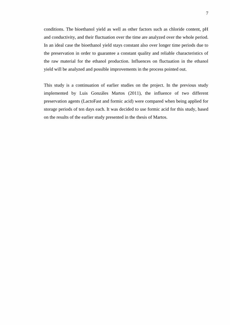
conditions. The bioethanol yield as well as other factors such as chloride content, pH

and conductivity, and their fluctuation over the time are analyzed over the whole period.

In an ideal case the bioethanol yield stays constant also over longer time periods due to

the preservation in order to guarantee a constant quality and reliable characteristics of

the raw material for the ethanol production. Influences on fluctuation in the ethanol

yield will be analyzed and possible improvements in the process pointed out.

This study is a continuation of earlier studies on the project. In the previous study

implemented by Luis Gonzáles Martos (2011), the influence of two different

preservation agents (LactoFast and formic acid) were compared when being applied for

storage periods of ten days each. It was decided to use formic acid for this study, based

on the results of the earlier study presented in the thesis of Martos.

8

3 BIOETHANOL

Ethanol, also called ethyl alcohol, is an alcohol derived from sugars by fermentation and

distillation. Therefore basically any feedstock containing a sufficient amount of sugar or

materials which can be converted into sugar is suitable for ethanol production. Referred

to as bioethanol is all ethanol obtained from biomass. (Schnepf 2006, 4-5.) According to

Demirbas (2006), bioethanol as an alternative fuel can be used either as a gasoline

additive or substitute and can be produced from wood, straw, crops and household

waste by the alcoholic fermentation of the sugars which are produced by hydrolysis of

the biomass. (Demirbas 2006, 1) Dependent on the feedstock for the production of

bioethanol, it can be referred to as a first generation or second generation biofuel. First

generation biofuels are produced from food crops, while second generation (or

advanced) biofuels are derived from non-food feedstocks, as can be seen in table 1.

(Demirbas, Balat & Balat 2011, 1817.)

TABLE 1. Classification of biofuels (Demirbas et al. 2011, 1817, modified)

Generation Feedstock Example

First generation biofuels Sugar, starch, vegetable

oils, or animal fats

Bioalcohols, vegetable oil,

biodiesel, biosyngas,

biogas

Second generation biofuels Non food crops, wheat

straw, corn, wood, solid

waste, energy crop

Bioalcohols, biooil, bio-

dmf, biohydrogen, bio-

fischer-tropsch diesel,

wood diesel

Third generation biofuels Algea Vegetable oil, biodiesel

Fourth generation biofuels Vegetable oil, biodiesel Biogasoline

Demirbas defines any biofuel as a ”non-polluting, locally available, accessible,

sustainable and reliable fuel obtained from renewable sources” (Demirbas 2008, 2106),

which makes them and especially bioethanol interesting in the future for the industry as

is explained more detailed in the following.

9

3.1. Bioethanol as an alternative fuel in the past, nowadays and in the future

Bio-ethanol, along with other biofuels, became increasingly interesting for research and

commercial production in the 1970’s after the first oil crisis which showed the need for

alternatives in cases of shortening in the oil supply. Fanchi and Fanchi present the

development of the the crude oil prize over the last 4 decades, where the first peak in

prize occurred in 1974. (Fanchi & Fanchi 2011, 87.)

Approximately at the same time the world reached the first peak oil point in 1978 and

first serious doubts about the limitless abundance of fossil fuels were raised. In figure 3

the world production rate of oil is presented along with a forecast of the future

production. The peak in the late 70’s as well as the prediction according to the

Gausssian curve can be seen.

FIGURE 3. World Oil Production Rate Forecast Using Gaussian Curve (Fanchi &

Fanchi 2011, 87)

Those two factors, the dependency on international trading and political relations as

well as the possible future shortage in oil and gas resources were therefore in the 1970’s

the main driving forces towards the development of biofuel production. Environmental

concerns about greenhouse gas emissions related to the use of fossil fuels were existent

already by that time, but became more important only later when the world policies

started to address environmental issues and especially the climate change as a result of

10

traffic- and industry-born air pollution. As stated by Türe, Uzun and Türe (1997), the

world-wide energy consumption grew 17-fold during the 20th

century and, resulting

mainly from the combustion of fossil fuels, CO2, SO2 and NOx became the main

causes of atmospheric pollution (Türe et al. 1997). The Kyoto protocol, signed in 1997

and put in force in 2005, as the first big international agreement on fighting global

warming, along with the oil peak being predicted for the time around the year 2000,

caused an increase in global biofuel production after 2000. In 2009, the EU published a

directive on the promotion of the use of energy from renewable sources in the European

Union, which contains a binding target of a share of 20 per cent of renewable energy by

2020 in the final energy consumption in the European Union. It also includes a binding

target for each member state of a minimum 10 per cent share of renewable energy

sources in transport. (Koponen, Soimakallio & Sipilä 2009, 3.) This directive is most

likely going to increase the pace of development of biofuel technologies even further.

Figure 4 shows the world-wide production of fuel ethanol from 1975 to 2003.

FIGURE 4. World and regional fuel ethanol production, 1975-2003, million liters per

year (Vessia 2005, 14)

Recently, bioethanol starts to become economically profitable and competitive with

fossil fuels and is according to Demirbas (2009) the world-wide most used biofuel. The

global production of bio-fuels was 68 billion l in year 2007, where the main feedstocks

for the bio-ethanol production are sugar cane, produced in Brazil with a 60 per cent

11

share of overall bio-fuel production, and other crops. (Demirbas, 2009, 2239.)

Nevertheless, even with the increasing oil prices, biofuels are still more expensive than

fossil fuels, but the biofuel industry is expected to be shaped in the coming century in

the same way the fossil fuel industry was shaped in the last century. Predictions for the

availability of modern transportation fuels are presented in table 2, where the

availability of bioethanol in the future is estimated to be excellent. Governments can

support this process with methods like for example the reduction of taxes on biofuels

and obligatory usage of biofuels. (Demirbas 2008, 2113.)

TABLE 2. Availability of modern transportation fuels (Demirbas 2009, 2240)

Fuel type Availability

Current Future

Gasoline Excellent Moderate-poor

Bioethanol Moderate Excellent

Biodiesel Moderate Excellent

Compressed natural gas Excellent Moderate

Hydrogen for fuel cells Poor Excellent

3.2. Application, restrictions and advantages of bioethanol fuel

Bioethanol as a fuel can be used according to the EU standard EN 228 as a 5 per cent

blend with petrol without any required modifications of the engine and in higher blends

of up to 85 per cent with engine modifications. In modern engines, E10 containing 10

per cent ethanol can be used. It is therefore a gasoline additive or substitute. The

environmental properties of bioethanol result in a net release of no carbon dioxide and

very little sulphur, due to a higher octane number, higher flame speed and evaporation

heat, and broader limits for flammability. These lead to a higher compression ratio and a

shorter burning time as well as leaner burn engine, which result in better efficiency in

internal combustion engines compared to petrol. Only anhydrous ethanol is suitable for

this use, while hydrated ethanol, containing more than 2 per cent of water, is only to

some extent miscible with gasoline and requires therefore further treatment. Bioethanol

which is produced biologically contains around 5 per cent of water and therefore falls

under this category. The energy density of ethanol is lower than that of gasoline.

Ethanol is more corrosive, has a lower vapour pressure which makes it more difficult to

start the engine in low temperatures, is miscible with water, and increases the emissions

12

of acetaldehyde and evaporating emissions when blending with gasoline. (Demirbas et

al. 2006, 2008, 2011.)

3.3. Sources of bioethanol

As it was said already earlier, ethanol can be won from any feedstock which can be

converted into sugars. Bioethanol is produced from renewable feedstocks. The value of

the biomass for the ethanol production is defined by how easily the conversion to sugars

takes place. This makes feedstocks with a high content of starch and sugars easily

convertible, while cellulosic materials require more pre-treatment. (Demirbas et al.

2011, 1818). Until now, mainly food crops are used for the bioethanol production, but

there is frequently active research done on the investigation of non-food crops as raw

materials due to different socio-economic effects such as increasing food prices,

shortages in food for cattle, and growing competition for land (Stichnothe & Azapagic

2009, 624)

3.3.1 Food crops

Food crops are suitable for the bio-ethanol production due to their high contents on fats,

proteins and carbohydrates. The production of bio-ethanol from food crops is criticized

due to the fact that its production reduces the resources for the food production and

therefore increases food prices. (Kessler 2008, 274-275) They are therefore referred to

as first generation bio-fuels, since they are sustainable only to a certain extent, as was

presented in table 1. Any food crop can be used for the ethanol production, but the

currently most used food crops are corn and sugar cane, where Brazil is the leading

ethanol producer using sugar cane, followed by the US deriving ethanol from corn.

(United States Department of Energy 2006, 39)

3.3.2 Common crops and lignocellulosic materials

Lignocellulosic materials are materials containing cellulose and lignin which are formed

during photosynthesis. They occur in wood as well as other woody tissue like for

example agricultural residues, grasses, and water plants. They are referred to as

13

biomass, but since biomass generally includes all kind of living substances,

lignocellulosic materials are just one specific form of biomass. (Rowell 1992, 12.)

Hu (2008) defines lignocellulosic materials as a “natural, abundant and renewable

resource”. Due to recent need for biofuels, lignocellulosic materials became

increasingly interesting as a raw-material for the production of such and especially in

the sector of bioethanol production. He also says that there are no effective and

economical ethanol production methods yet due to a lack of knowledge about the

structures of lignocellulosic materials, and that improved methods for their

characterization still need to be developed. (Hu 2008)

There are different lignocellulosic materials used for the bioethanol production. One

example is woodchips, the residues of the forest and timber industry in form of scraps

of tree stems, shredded twigs and similar. Another lignocellulosic material used is

agricultural waste material, which is the leftovers of agricultural production of crops

and represents the remaining part of the plants which are of no use for the food industry

or others (Najafi et al., 2008). Research is lately done on the usage of different grasses,

like for example switchgrass, a grass growing in North-America and Canada having

high contents of cellulose and growing very high, making it a suitable feedstock for

ethanol production (Rinehart 2006, 1). Another grass used is Miscanthus, which is also

a high yielding energy crop and only recently being researched for the use for

bioethanol production. (Sørensen et al. 2007, 6602)

3.3.3 Municipal waste

According to Stichnothe and Azapagic (2009), municipal waste and especially organic

waste becomes due to its qualities increasingly interesting for the energy production

industry, since the environmental and economical benefits of bioethanol derived from

cultivated crops are questionable. Waste materials used as feedstock for the bioethanol

production decrease the stress on landfills, increase the re-use of materials and reduce

the greenhouse gas emissions from landfill sites. By this they help to fulfil requirements

of legislations such as the European Waste Framework Directive. (Stichnothe &

Azapagic 2009, 624)

14

The production of bioethanol from biowaste has been researched only little until now

and therefore needs further investigation. In the study from Stichnothe and Azapagic

(2009), the greenhouse gas emissions of the production process of bioethanol from both

household waste Refuse Derived Fuel and Biodegradable Municipal Waste was

analyzed with the result, that even though the production of bioethanol from RDF

reduces emissions compared to current waste management practice in the UK, it

nevertheless does not save any emissions when comparing the RDF derived ethanol fuel

with petrol. On the other hand, there is a reduction in greenhouse gas emissions of 92,5

per cent from the fuel combustion process comparing the ethanol produced from BMW

with petrol. Bioethanol derived from Brazilian sugar cane reached only savings of up to

70 per cent compared to petrol. (Stichnothe & Azapagic 2009, 624.) This makes the

biodegradable waste, which is analyzed in this study at TAMK, especially interesting as

a future raw material for the fuel ethanol production.

3.4. Production of bioethanol

According to Demirbas et al. (2006), the process of deriving ethanol from biomass

consists of two main steps: the hydrolysis of carbohydrates to simple sugars glucose and

xylose, and the fermentation of the sugars to alcohol. Carbohydrates can be the cellulose

and hemicellulose in plant matter for example. Cellulose is an organic polymer which

occurs in long molecular chains, consisting of units of anhydro glucose. During

hydrolysis it is split up into glucose, where the conversion efficiency is dependent

mostly on the chemical and mechanical pre-treatment of the cellulose. Hemicelluloses

occur in much shorter chain molecules than cellulose and act as bindings between the

cellulose molecules. They are soluble in alkali, which enhances the hydrolysis. The

hemicelluloses occurring in woody tissues break down much easier during thermal

treatment. (Demirbas et al. 2006, 9.)

The enzymatic hydrolysis process is presented in figure 5, where after the hydrolysis of

the carbohydrates with the help of acid and cellulase enzymes both the C5 and C6-sugars

are fermented and the resulting ethanol is distilled to obtain higher concentrations.

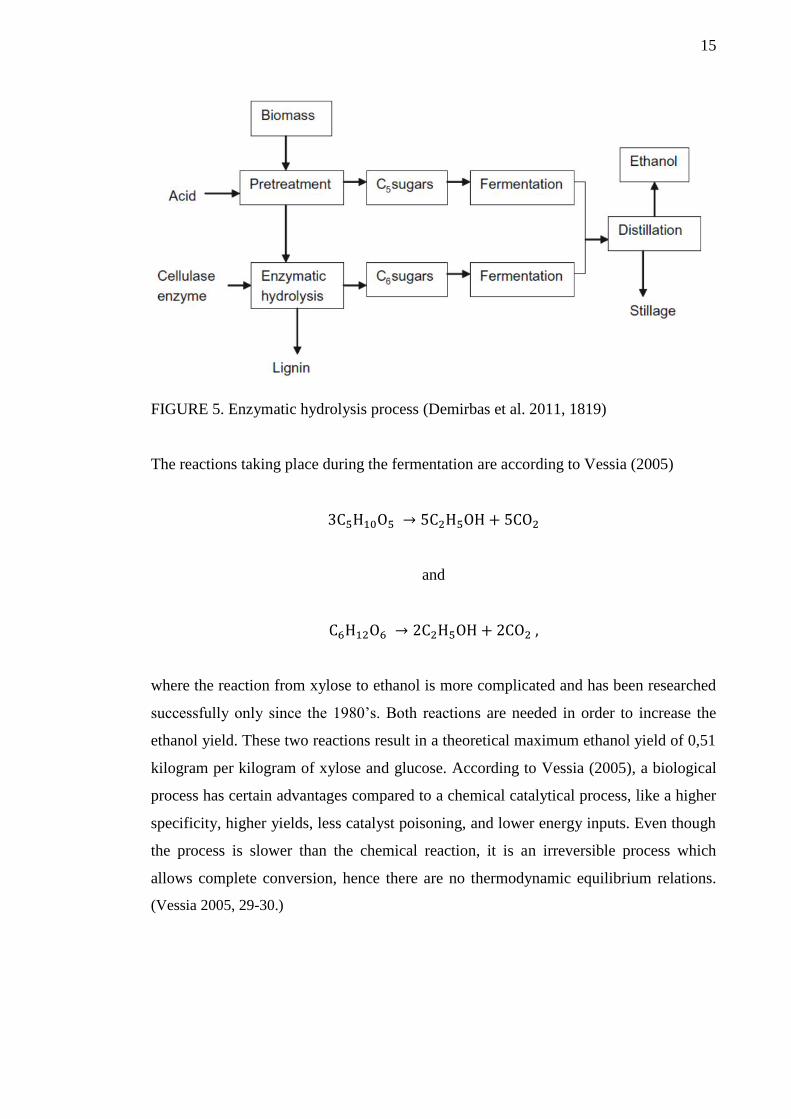
15

FIGURE 5. Enzymatic hydrolysis process (Demirbas et al. 2011, 1819)

The reactions taking place during the fermentation are according to Vessia (2005)

and

where the reaction from xylose to ethanol is more complicated and has been researched

successfully only since the 1980’s. Both reactions are needed in order to increase the

ethanol yield. These two reactions result in a theoretical maximum ethanol yield of 0,51

kilogram per kilogram of xylose and glucose. According to Vessia (2005), a biological

process has certain advantages compared to a chemical catalytical process, like a higher

specificity, higher yields, less catalyst poisoning, and lower energy inputs. Even though

the process is slower than the chemical reaction, it is an irreversible process which

allows complete conversion, hence there are no thermodynamic equilibrium relations.

(Vessia 2005, 29-30.)

16

4 EXPERIMENTAL STUDIES

4.1. Implementation of the experiment

The experimental set-up was the same as in the two previous studies on this project

implemented by Esther Posadas Olmos (2011) and Luis Gonzáles Martos (2011). In the

facilities of the TAMK laboratories a vessel, which can be seen in figure 6, with a

volume of 0,8 cubic meters provided and patented by Aate Virtanen was installed and

tested within the Jäte-Aate project at TAMK since 2010 over periods of two weeks for

the anaerobic storage of preserved biowaste. Kitchen waste is fed to the vessel via a

grinder (model imc 726) which can be seen in figure 7 with addition of water in order to

ensure that the waste does not block the pipe. Samples of the vessel content can be

taken from two valves at different heights on the vessel. Pressure as well as temperature

is measured constantly, and a valve on the top of the vessel allows the measurement of

the gas composition inside the vessel.

17

FIGURE 6. Biowaste preservation installation in the TAMK greenhouse (Photo: Luis

González Martos 2011)

FIGURE 7. Structure of the feeding grinder (Photo: Luis González Martos 2011)

18

Waste was collected from the TAMK cafeteria, where it was stored in an air-

conditioned room outside the kitchen, and brought in closed buckets to the laboratories.

This was done twice a week in the time from 1.11.2011 until 31.1.2012 aiming at

collecting a waste mass of 40 kilograms a week dependent on the quality of the

available kitchen waste. Large amounts of paper waste were avoided since they could

have caused possible blockings of the feeding grinder. There were slight fluctuations in

volumes of waste fed to the vessel over the time due to an occasional lack of useable

waste. The waste was composed of food products, where salad, potato products and

grain products were dominating components. An accurate list of all materials added can

be found from the appendix 2 of this thesis.

In total a minimum of 400 kilograms of waste had to be collected during the period of

three months. While in the previous studies the testing periods lasted only for a few

weeks, this time the changes in the bioethanol yield over a longer time period were

studied.

The collected waste was weighed and preserved using liquid formic acid AIV 2 plus in

a ratio of 5 millilitres per kilogram of waste. The material safety data sheet of the

product is included in the appendix 1 of this thesis. The formic acid was handled under

the hood using a volumetric pipette. After the addition of the formic acid the waste was

mixed thoroughly and screened in order to avoid feeding accidently disposed non-

biodegradable or too large pieces into the grinder. The water flow was kept below 0,5

litre per kilogram of waste in order not to dilute the raw material too much.

Nevertheless it was sometimes needed to exceed this limit when the material was too

dry, other times, when having rather moist waste samples, much less water was used.

The overall addition of water stayed therefore within the given range.

The pH of the vessel content was measured three times a week with a Mettler Toledo

pH meter when sampling the preserved biowaste. pH measurements were done

according to the international standard ISO10390. Samples of the vessel content could

be measured straight with the instrument, whereas the biowaste samples had to be

diluted with distilled water (dilution factor 1:5) and stirred for at least 15 minutes before

measuring the pH.

19

The conductivity of the preserved biowaste was measured three times a week using a

Mettler Toledo conductivity meter.

The gas composition inside the vessel was measured three times a week with the help of

the Gas Analyzer Geotech GA 2000PLUS. The instrument was measuring CH4, O2, and

CO2 content.

4.2. Analytical methods

After the implementation of the testing period of three months, the samples taken during

that time were analyzed regarding their bioethanol yield and their chloride content. Not

all samples taken during the testing period could be analyzed due to a tight schedule. It

was decided to use for the analysis two samples of the first month of the experiment,

and four samples of each the second and third month, since it was more interesting to

see the development of the ethanol potential during later stages of the experiment. The

bioethanol yield was analyzed using the testing procedure described below, including

also the measurement of pH and dry matter content of the samples before and after the

fermentation process. The chloride content of the samples was measured using

potentiometric titration as is described in chapter 4.2.2.

4.2.1 Bioethanol potential

The basic principle of the bioethanol potential test is the hydrolysis of carbohydrates to

sugars and the fermentation of the glucose in the raw material, and the calculation of the

ethanol produced by the determination of the loss in weight of the raw material during

the fermentation. In order to make the glucose in the raw material available for

fermentation, enzymes were used which degrade the long-chained starch in the sample.

Acid Alpha Amylase GC 626 and Glucoamylase Diazyme® SSF2 were used for this

purpose. The influence of the α-Amylase in combination with a suitable pre-treatment

temperature on the ethanol yield can be seen from figure (Genencor 2010).

20

FIGURE 8. Impact of pre-treatment on final ethanol yield (Genencor 2010)

The procedure used for analyzing the bioethanol yield was based on a study comparing

different treatment methods (Lemuz et al. 2009, 356), and adjusted according to the

instruction on the dosages of enzymes and yeast recommended by the producers of the

products. The resulting procedure was applied equally to all samples.

First, the pH of the samples was adjusted to 4.25 at room temperature using 0.5M

NaOH. 3-4 replicates of each sample, according to the initial volume of sample

available, with a volume of 80-100 millilitres were placed in 250 or 300 millilitre

Erlenmeyer flasks and 5.24 micro litres of α-Amylase per 10 millilitres of sample

added. The samples were then heated and kept at 65ºC in a water bath (see figure 9) for

one hour while swirling them regularly. After that, 14.6 micro litres of glucoamylase

per 10 millilitres of sample were added and the flasks swirled again to mix the sample.

The samples were then left to cool down, and at a temperature below 32ºC 0.05 grams

of fresh yeast per 10 millilitres of sample were added. The samples were again mixed

well and the flasks closed with water locks. pH and dry matter content of the samples

were determined, as well as the initial weight of each Erlenmeyer flask and content.

21

FIGURE 9. Water bath with ethanol samples (Photo: Magdalena Gerlach 2012)

FIGURE 10. Barnstead|Lab-Line MaxQ 2000 Shaker (Photo: Magdalena Gerlach 2012)

The samples were then left for 72 hours for fermentation on a Barnstead|Lab-Line

MaxQ 2000 Shaker, as presented in figure 10, at 150rpm. Every four hours, if possible,

the samples were weighed again and the reduction in mass monitored. After 72 hours

the final mass was determined and again pH and dry matter content analyzed. The total

reduction in mass defines the reaction of glucose to ethanol, so that the amount of

ethanol produced can be calculated as can be seen in the results part of this thesis.

22

4.2.2 Chloride content

The chloride content defines the quality of the raw material for bioethanol production

significantly. Due toindustrial process related reasons, the material is required to have a

chloride content of below 1%.

The chloride content was analysed according to the International standard SFS-EN ISO

5943 by potentiometric titration of the preserved food waste. In order to obtain the total

chloride stored also in the solid parts of the raw materials which are not dissolved, a

standard for the analysis of milk products was applied.

Four samples from different stages of the testing period were analysed by using the

automated titrator Mettler Toledo DL50 as can be seen in figure 11. Three replicates of

each sample were taken. A dilution of the raw material with distilled water in a ratio 1/5

due to the thickness of the raw material was necessary in order to get analysis results.

FIGURE 11. Mettler Toledo DL50 (available at

http://www.globalspec.com/NpaPics/42/92833_110420036371_ExhibitPic.jpg,

accessed 24.4.2012)

23

5 RESULTS AND CONCLUSIONS

5.1. Presentation of the measurements

In the following there are the measurements and analyses which were conducted during

and after the testing period presented, as well as possible reasons for the results

analyzed. An overview of the measurements taken during the testing period can be

found from appendix 3.

5.1.1 pH of the preserved biowaste

The pH was measured over the whole testing period starting from day 17. It was kept

around 3,5 over the whole period by the addition of the formic acid. The reason for this

procedure was the prevention of the formation of microorganisms in the vessel which

would support the fermentation of the food waste when it is not desired yet. The pH was

successfully kept low and did not vary significantly as can bee seen from figure 12. The

small raise of the pH in the end of the testing period could be a result of the last addition

of food waste, which was with 40 kilograms rather big compared to earlier additions of

usually around 20 kilograms at a time.

FIGURE 12. pH development over the testing period

0

1

2

3

4

5

6

7

0 10 20 30 40 50 60 70 80 90 100

pH

Day

pH development

24

5.1.2 Conductivity of the preserved biowaste

According to the United States Environmental Protection Agency, the conductivity is “a

measure of the ability of water to pass an electrical current”, which results from

inorganic or organic compounds dissolved in the water, where the inorganic

compounds, like also the chloride, conduct easily electric charges and result therefore in

higher conductivity, and organic compounds lower it. (EPA 2012).

It stayed, as also the pH, rather stable around 12 milli Siemens per centimetre as can be

seen from figure 13. It was not influenced from outside and is a result of the

composition of the vessel content.

FIGURE 13. Conductivity development over the testing period

5.1.3 Gas composition inside the vessel

The gas composition inside the vessel gives information about the reactions happening

in the preserved biowaste. The most interesting gas to observe is the carbon dioxide,

since it is formed as a result of the fermentation in the vessel. As can be seen in figure

14, the carbon dioxide content was peaking three times during the testing period. It was

raising nearly linearly during the first 40 days of the experiment to drop then very

0

2

4

6

8

10

12

14

16

18

20

0 10 20 30 40 50 60 70 80 90 100

Co

nd

uct

ivit

y [m

S/cm

]

Day

Conductivity development

25

rapidly. Simultainously, the oxygen content was raising. This can be explained only by

the fact that someone must have opened the vessel cover. Otherwise oxygen could have

neither entered the vessel nor is there any reaction which possibly could have resulted in

oxygen being formed. The oxygen content went back to close to zero per cent within

only 15 days again. At the same time the carbon dioxide was rising steeply again up to

nearly 60% to slowly go down then again, and was rising in the end of the testing period

again up to nearly 70%. In the following it has to be examined what was causing the

rise in carbon dioxide, and if the feeding procedure of the biowaste to the vessel could

possibly have an effect on the early fermentation. The methane content stayed close to

0% over the whole testing period as was desired, which indicates that no anaerobic

digestion took place.

FIGURE 14. Gas composition inside the vessel over the testing period

5.1.4 Chloride content of the preserved biowaste

The chloride content was given by the Mettler Toledo DL 50 in grams per litre of

sodium chloride as can be found from the appendix 4-7, which needed to be converted

into the concentration of chloride only. The sodium chloride compound has a molar

mass of 58,44 grams per mole, out of which the Sodium is responsible for 22,99 grams

per mole, and the chloride for 35,45 grams per mole. The chloride has therefore a

0

10

20

30

40

50

60

70

80

0 20 40 60 80 100

Co

nce

ntr

atio

n [

%]

Day

Gas composition development

CH4

CO2

O2

26

percentage of the overall mass of 60,6. The concentration was then converted as

follows:

Dilution factors were taken into account where they had been used, and the average of

the three replicates was calculated. The results are presented in table 3. As it can be

seen, the chloride content did vary only between 0,179 and 0,207 per cent over the

whole testing period. Given a requirement of a chloride content of the raw material

below 1 per cent, these results are more than favourable in this sense.

TABLE 3. Chloride content of the preserved biowaste

Day of the

experiment

Date Chloride conc.

[g/l]

Chloride conc.

[%]

24 24.11.11 2,068 0,207

58 28.12.11 1,791 0,179

79 18.1.12 1,886 0,188

92 31.1.12 1,793 0,179

5.1.5 Dry matter content of the preserved biowaste

Unfortunately the results for the dry matter content are questionable as the

measurements were fluctuating crucially, up to over 9 per cent over a time span of only

two weeks, and can therefore be used for interpretation only to a certain extent. Rough

conclusions have to be drawn from the results available.

The fluctuation of the results might have several reasons. One possible explanation is

that the fluctuating values are a result of the analysis method, which works with very

small sample sizes around 1 gram. The small sample size means that the sample is not

fully representative for the original sample, since the solid content of the raw material,

although grinded when added, is not dissolved in the water. The dry matter content of

the small sample taken can therefore vary tremendously. Due to limited time resources

it was not possible to analyse more replicates. It would have been more favourable to

conduct the analysis with a standard gravimetric method for determination of dry matter

27

content which uses bigger sample sizes. The standard method SFS-EN 12145 could be

used for example.

The sampling from the vessel had an influence on the dry matter content of the sample

as well. Inside the vessel, the solid is suspected to separate from the liquid and settle at

the bottom of the vessel. This hypothesis is supported by the fact that the samples taken

during the first weeks were rather liquid and started to contain solids only after a few

weeks, when the level of the vessel content was rising. Once the solid level had reached

the outlet valve, it was noticed that from time to time the valve got blocked and the

texture of the sample became more liquid again. This does not affect the dry matter

content analysis as such, but makes it more difficult to draw conclusions on the relation

between time, dry matter content and bioethanol potential.

The dry matter content as it was measured before and after the fermentation of the

samples is presented in figure 15. It is assumed that the first peak in the dry matter

content before the fermentation is an outlier and does not represent the real situation.

FIGURE 15. Dry matter content over the testing period

In order to make in the following parts of this work assumptions based on the dry matter

content, trendlines have been drawn for the dry matter content after fermentation which

allow to calculate rough values of the dry matter content over the whole testing period.

0

2

4

6

8

10

12

0 20 40 60 80 100

Dry

mat

ter

con

ten

t [%

]

Day

Dry matter content development

Dry matter content before fermentation

Dry matter content after fermentation

Linear (Dry matter content before fermentation)

28

The equation for the dry matter content based on the trendline before fermentations is:

where x is the day of sampling. This trend is also only approximate since it is based on

the measurement results. Furthermore it could be assumed that the rising of the dry

matter content follows, in contrast to the proposed linear trend, in reality rather an

exponential trend with progressing time, since the settling of the dry matter follows the

rule of gravity and it therefore can be assumed that from bottom to the top the speed of

settling as well as the density of the raw material decreases. Nevertheless the drawn

trend lines seem to be reasonable compared to the measurement results and will

therefore be used.

5.1.6 Ethanol yield

In order to analyze the ethanol yield, the mass loss of the samples during the 72 hours of

the fermentation process was studied as described in chapter 4.2.1. The results of the

change in mass over the time are presented in figure 16. In the measuring procedure,

two samples could be analyzed at a time, and the results show that there is no visible

correlation between the mass loss behaviour and the analysis session. Several samples

had infrequently a little raise in the mass where it was expected to decline constantly.

One possible reason for this behaviour could be the scale itself in case it was used by

others in between the measurements and somehow moved or in some other way

influenced. This theory is supported by the fact that the changes could be seen in many

cases similarly at the same time in all replicates analyzed at a time, as for example can

be seen in the samples from day 24 and 29, which both gained in mass after around 48h

of fermentation. Another possible reason is the dropping of water from the water locks

on top of the Erlenmeyer beakers used. For the first analysis session there were water

locks used which apparently did not always prevent the water from dropping into the

sample. The amounts of water added to the sample were small, but nevertheless crucial

for the total mass loss. Affected samples were excluded from the calculation of the

average.

29

FIGURE 16. Comparison of the mass loss in grams per 100 grams of raw material in the

ethanol samples

The ethanol which was produced during fermentation was calculated from the loss in

mass. It is known that the reaction from glucose to ethanol and carbon dioxide results in

a quantitative mass of 0,51 grams of ethanol and 0,49 grams of carbon dioxide per gram

of glucose.

The reaction from glucose to ethanol is described as:

(Dien 2010, 218)

Therefore the loss in mass of the sample represents the amount of carbon dioxide being

formed during fermentation, and could be transferred into the conversion rate of

0,0

0,2

0,4

0,6

0,8

1,0

1,2

0 10 20 30 40 50 60 70 80

Mas

s lo

ss [

g/1

00

g sa

mp

le]

Hours

Mass loss in the samples

Day 24

Day 29

Day 37

Day 44

Day 49

Day 58

Day 65

Day 72

Day 81

Day 92

30

biomass to ethanol. In table 4, the measurements of dry matter content before and after

fermentation as well as the ethanol yields in grams per 100 grams of wet sample are

presented. It becomes clear that there was in nearly all cases a reduction in the dry

matter content, which indicates along with the mass loss that solids were decomposed

and fermentation took place.

TABLE 4. Analyses done after the testing period (dry matter content of the sample

before and after fermentation, ethanol produced)

Day

DM before

fermentation

[%]

DM before

fermentation

(calculated)

[%]

DM after

fermentation

[%]

Ethanol yield

[g/100g of wet

sample]

24 2,78 3,98 2,64 0,028

29 10,81 4,43 0,53 0,006

37 3,44 5,15 1,84 0,019

44 1,35 5,78 0,34 0,004

49 3,41 6,23 1,64 0,017

58 10,31 7,04 7,54 0,079

65 8,10 7,67 3,24 0,034

72 8,82 8,3 4,15 0,043

81 9,72 9,11 3,10 0,032

92 10,16 10,1 6,50 0,068

The results for the ethanol yield of the wet samples in grams of ethanol per 100 grams

of sample are presented in figure 17. As can be seen from the graph, the ethanol yield

was reaching its peak on the 58th day of the experiment with 0,079 grams of ethanol per

100 grams of sample, after being close to zero only two weeks before that. After the

peak the ethanol yield declines again to 0,043 grams of ethanol per 100 grams of

sample, but raises at the end of the experiment again.

31

FIGURE 17. Ethanol produced in grams per 100 grams of the samples

Unfortunately it was not possible to determine the glucose content of the raw material.

It would have been interesting to define the conversion rate of glucose to ethanol.

5.2. Conclusions on the ethanol yield results

There can be many reasons for the behaviour of the ethanol yield, out of which only a

few can be analysed in this study. The correlation between the ethanol yield and the

carbon dioxide being emitted during the experiment is observed, as well as the

correlation between ethanol yield and the dry matter content of the raw material. In

addition, the amounts and times of the adding of raw material to the vessel will be

analysed in order to find a possible influence on the ethanol potential.

The carbon dioxide content of the gas composition inside the vessel, as already said,

was fluctuating irregularly. This is supposed to be an indicator for early fermentation.

When looking at figure 18, which presents both the carbon dioxide content and the

change in ethanol yield in grams per 100 grams of sample, there nevertheless does not

seem to exist a clear correlation between those two measurements.

0

0,01

0,02

0,03

0,04

0,05

0,06

0,07

0,08

0,09

0 10 20 30 40 50 60 70 80 90 100

Eth

ano

l pro

du

ced

[g/

10

0g

of

sam

ple

]

Day

Ethanol yield

32

FIGURE 18. Correlation between ethanol yield of the samples and CO2 emitted

The dry matter content of the raw material is much likely to have an influence on the

bioethanol potential. A study conducted by Byung-Hwan and Hanley (2008) on the

ethanol yield and conversion of lignocellulosic biomass by conventional fermentation

showed that the best conversion was achieved with a dry matter content of 10 per cent

as can be seen in table 5. In the study there was used Zyomonas mobilis, and the

fermentation took place for 48h. Tested were solid concentrations of 10, 15 and 20 per

cent. (Byung-Hwan & Hanley 2008, 1257-1265.) These results are comparable only to

some extend to this study case, since the used biomass was different, but nevertheless it

could be expected that this tendency is applicable for all raw materials.

0

10

20

30

40

50

60

70

80

0

0,01

0,02

0,03

0,04

0,05

0,06

0,07

0,08

0,09

0 20 40 60 80 100

CO

2 [

%]

Eth

ano

l pro

du

ced

[g/

10

0g

of

sam

ple

]

Day

Correlation between ethanol yield and CO2 content

Ethanol yield of the samples

CO2 content

33

TABLE 5. Ethanol yield and conversion in per cent by Z. mobilis after 48 h (Byung-

Hwan & Hanley 2008, 1264)

Substrate

concentration

10% 15% 20%

Initial glucose after

enzyme reaction

[g/l]

42.6 55.5 58.4

Final ethanol

concentration after

48h [g/l]

18.2 19.7 6.3

Conversion of

consumed glucose

into ethanol [%]

83.6 73.4 21.8

Theoretical ethanol

yield [%]

80.5 68.6 19.1

Total fermentation

time based on

portion method [h]

106 110 114

Comparing the ethanol yield obtained in this study to the dry matter content as can be

seen in figure 19, it can be said that there is some correlation between them. The dry

matter values obtained by calculation according to the trend line were used, which were

presented earlier. It is assumed that the tremendous fluctuations in the ethanol yield are

a result of the analysis method. The analysis method includes a big number of

influencing factors like the yeast, enzymes, temperature of the water bath and others,

which make the results very vulnerable. Nevertheless there can still be seen a slight

raise in the ethanol yield over the time between those fluctuations, which seems nearly

linear with the calculated dry matter content. Unfortunately the dry matter content did

not rise above 10 per cent. It is therefore not known if the conversion would have

grown further on with higher dry matter content or declined again as the study of

Byung-Hwan and Hanley (2008) showed.

34

FIGURE 19. Correlation between the ethanol yield of the samples and the dry matter

content

Looking at the addition of food waste to the vessel presented in figure 20, it can be seen

that there were two short breaks in the feeding rhythm; one around the 40th day of the

experiment due to a lack of available biowaste, and another longer break around the

60th day of the testing period resulting from the Christmas holiday during which the

TAMK kitchen was out of service. It can be seen that additions of biowaste exceeding

20-25 kilograms resulted in peaks in the ethanol potential, while breaks in the adding

lead to a decrease in ethanol yield. This is an interesting observation since the addition

of the acid and the dilution with water in combination with the grinding should result in

a rather homogenous mixture of the waste inside the vessel. The peaks did not show

immediately after the additions but only some days later, which also precludes the

assumption of the food waste not having settled down yet which could influence the

sample.

0

2

4

6

8

10

12

0

0,01

0,02

0,03

0,04

0,05

0,06

0,07

0,08

0,09

0 20 40 60 80 100

DM

[%

]

Eth

ano

l pro

du

ced

[g/

10

0g

of

sam

ple

]

Day

Correlation between ethanol yield and dry matter content

Ethanol yield of the samples

Calculated dry matter content

35

FIGURE 20. Correlation between the ethanol yield of the samples and the amounts of

biowaste added

0

5

10

15

20

25

30

35

40

45

0

0,01

0,02

0,03

0,04

0,05

0,06

0,07

0,08

0,09

0 20 40 60 80 100

Bio

was

te a

dd

ed

[kg

]

Eth

ano

l pro

du

ced

[g/

10

0g

of

sam

ple

]

Day

Correlation between ethanol yield and amounts of biowaste added

added biowaste

Ethanol yield of the samples

36

6 DISCUSSION

The study showed that it is possible in general to store the preserved biowaste over 3

months without losing the properties needed for bioethanol production. Further on it

should be studied whether even longer periods of storage for this purpose would be

possible. The qualities of the pre-served biowaste concerning pH, conductivity and

chloride content were as desired, meaning stable values for the pH and the conductivity

without fluctuations, and a chloride concentration of below 1 per cent over the whole

testing period, which makes it easier to focus on other possible reasons for the

fluctuations in the bioethanol yield. In this study it could not yet be fully investigated

how efficient exactly the hydrolysis and fermentation procedures were, as well as the

factors influencing the processes, and thus how valuable the preserved biowaste is as

raw material.

The dry matter content seems to have an influence on the bioethanol yield, as was also

confirmed by the study of Byung-Hwan and Hanley (2008, 1264), but unfortunately

only solid contents of up to 10 per cent could be achieved with the procedure applied in

this study. It would have been interesting to know how the ethanol yield changes for

higher solid contents. The addition of water during the feeding process of the biowaste

had maintenance-related reasons, and it needs to be determined if it is possible even to

reduce the volumes of water added without causing problems to the grinder. However,

the dry matter content itself was not the problem in this study but inaccuracies in the

measurement procedure. For the future, a method should be applied using bigger sample

volumes in order to obtain more reliable results.

There were fluctuations in the carbon dioxide content inside the vessel, which might

stand in some correlation to the bioethanol yield. This correlation needs to be further

investigated and also possible reasons for the changes in the carbon dioxide content

examined. There is a possibility that the addition of the biowaste has an influence on the

carbon dioxide content, and maybe even the bioethanol yield directly, when the feeding

rhythm was irregular or the masses of biowaste added were varying. The impacts of the

adding behaviour should be analyzed further on.

37

To make the results more comparable to already existing data, it would be necessary to

analyze also the glucose content of the preserved biowaste. Nevertheless the conversion

rate of the raw material to ethanol is of main interest for ethanol producers.

Comparing the obtained results on the ethanol yield with already existing studies, it

becomes clear that the ethanol yield obtained with our procedure is relatively small.

Kim et al. (2008) analyzed in their study the optimization of enzymatic saccharification

and ethanol fermentation of food waste with the help of a statistical model and

experimental verification. Food waste of a university cafeteria was used in the study of

Kim et al. (2008), and its composition can be assumed to be similar as the composition

of the raw material used in the Jäte-Aate project. In the study of Kim et al. (2008), the

food waste was diluted with water in a ratio 1:1, resulting in a dry matter content of 12,9

per cent. The resulting optimum conditions for the hydrolysis were according to Kim et

al. (2008) a pH of 5,20 and an enzyme reaction temperature of 46,3°C. For the

fermentation the optimum conditions were found to be a pH of 6,85 and a temperature

of 35,3°C. The enzyme which was used was glucoamylase, with an optimum

concentration of 0,16 per cent. Ethanol fermentation was conducted in anaerobic

conditions, handling the samples in a vacuum anaerobic chamber. (Kim et al. 2008,

1308.) Comparing these conditions to the procedure applied in the study conducted at

TAMK, it can be seen that even though there are some similarities, the methods

nevertheless differ. The enzyme concentration used in this study was with 0,146 per

cent very similar to the optimum concentration found by Kim et al. (2008). The reaction

temperature for the glucoamylase should have been similar, since the glucoamylase was

added after taking the samples out of the waterbath in the Jäte-Aate study, hence when

cooling down from 65°C to room temperature. Fermentation took place at room

temperature, which was around 21°C and therefore below the optimum 35,3°C found by

Kim et al. (2008). The maximum ethanol yield obtained with the optimized method by

Kim et al. (2008) was 57,6 grams of ethanol per litre of raw material. Comparing this to

the maximum yield obtained in the Jäte-Aate study of around 0,79 grams of ethanol per

litre of diluted waste (assuming a density of around 1 kilogram per litre), the deficit in

the used method becomes clear.

It can be said that the rather low ethanol yield results were achieved due to a lack of

insufficient knowledge in this field. The ethanol production method by hydrolysis and

38

fermentation is a biological process, which is influenced by a huge variety of factors.

Their influences have to be studied further on. The Jäte-Aate vessel in the TAMK

laboratories provides a suitable frame to study the behaviour of the bioethanol yield and

different influencing factors on the process, so that the system could be improved

further on. In general the Jäte-Aate vessel seems suitable for the production of raw

material, which can be converted into bioethanol. Therefore the Jäte-Aate vessel should

be further improved for on-site applications.

39

REFERENCES

Byung-Hwan, U. & Hanley, T.R. 2008. High-Solid Enzymatic Hydrolysis and

Fermentation of Solka Floc into Ethanol. Journal of Microbiology and Biotechnology,

Volume 18, Issue 7, 2008, 1257–1265

Ciscochem.Material Safety Data Sheet of Formic Acid. 01.02.2011 [available at

http://www.ciscochem.com/msds/files/Formic_Acid.pdf]

Demirbas, A., 2006. Progress and recent trends in biofuels. Progress in Energy and

Combustion Science, Volume 33, 2007, p. 1-18

Demirbas, A., 2008. Biofuels sources, biofuel policy, biofuel economy and global

biofuel projections. Energy Conversion and Management, Volume 49, 2008, p. 2106-

2116

Demirbas, A., 2009. Biofuels securing the planet’s future energy needs. Energy

Conversion and Management, Volume 50, 2009, p. 2239-2249

Demirbas, M. F., Balat, M. & Balat, H., 2011. Biowastes-to-biofuels. Energy

Conversion and Management, Volume 52, Issue 4, April 2011, p. 1815-1828

Dien, B. S., 2010. Mass Balances and Analytical Methods for Biomass Pretreatment

Experiments. In: A. A. Vertès et al., ed. 2010. Biomass to Biofuels. Strategies for

Global Industries. Chippenham: Wiley

Fanchi, J. R., Fanchi, C. J., 2011. Energy in the 21st Century (2nd Edition). Singapore:

World Scientific Publishing Co. Pte. Ltd.

Foerster, H. 2010. Granular Starch Hydrolysis (GSHE) for Conversion of Grains to

Ethanol, Near-term Opportunities for Bio refineries Symposium. Genecor. IL,

Champaigne

Hu, T. Q., 2008. Characterization of Lignocellulosic Materials. Wiley-Blackwell

Kessler, E., 2008. Our Food and Fuel Future. In: D. Pimentel, ed. 2008. Biofuels, Solar

and Wind as Renewable Energy Systems. Benefits and Risks. NY: Springer, 274-275

Khanal, S. K. et al., 2010. Bioenergy and Biofuel from Biowastes and Biomass.

Virginia: American Society of Civil Engineers.

Koponen, K., Soimakallio, S. & Sipilä, E., 2009. Assessing the greenhouse gas

emissions of waste-derived ethanol in accordance with the EU RED methodology for

biofuels. VTT Research Notes 2507. Helsinki: Edita Prima Oy

Lemuz et al. 2009. Development of an Ethanol Yield Procedure for Dry-Grind Corn

Processing. Cereal Chemistry, Volume 86, Issue 3, p. 355.360

40

Martos, L. G., 2011. Preservation of bio-waste for reuse. Bachelor’s thesis. Tampere

University of Applied Sciences.

Najafi, G., Ghobadian, B., Tavakoli, T. & Yusa, T., 2008. Potential of bioethanol

production from agricultural wastes in Iran. Renewable and Sustainable Energy

Reviews, Volume 13, Issues 6-7, August-September 2009, p. 1418-1427

Oliveira, L. S., Franca, A. S., 2009. From Solid Biowastes to Liquid Biofuels. In:

Ashworth, G. S., Azevedo, P., eds. 2009. Agricultural Wastes. Nova Science Publishers,

Inc. Chapter 11.

Olmos, E. P., 2011. Preservation of biowaste for reuse (Prebiore). Bachelor’s thesis.

Tampere University of Applied Sciences.

Rinehart, L., 2006. Switchgrass as a bioenergy crop. NCAT

Rowell, R. M., 1990. Opportunities for Lignocellulosic Materials and Composites. In:

Emerging technologies for materials and chemicals from biomass: Proceedings of

symposium. Washington, DC: American Chemical Society, 1992, Chap. 2. ACS

symposium series 476

Schnepf, R., 2006. Agriculture-Based Renewable Energy Production. In: V. I.

Welborne, ed. 2006. Biofuels in the Energy Supply System. New York: Nova Science

Publishers, Inc., 4-5

Stichnothe, H., Azapagic, A., 2009. Bioethanol from waste: Life cycle estimation of the

greenhouse gas saving potential. Resources, Conservation and Recycling, Volume 53,

2009, p. 624-630

Sørensen, A., Teller, P. J., Hilstrøm, T. & Ahring, B. K., 2007. Hydrolysis of

Miscanthus for bioethanol production using dilute acid presoaking combined with wet

explosion pre-treatment and enzymatic treatment. Bioresource Technology, Volume 99,

Issue 14, September 2008, p. 6602–6607

Türe, S., Uzun, D. & Türe, I. E., 1997. The Potential Use of Sweet Sorghum as a Non-

Polluting Source of Energy. The International Journal of Energy, Volume 22, 1997, p.

17-19

United States Department of Energy, 2006. Biofuels-at-a-Glance. In: V. I. Welborne,

ed. 2006. Biofuels in the Energy Supply System. New York: Nova Science Publishers,

Inc., 39

United States Environmental Protection Agency, 2012. Conductivity. [available at

http://water.epa.gov/type/rsl/monitoring/vms59.cfm]

Vessia, Ø., 2005. Biofuels from lignocellulosic material. Trondheim: Norwegian University

of Science and Technology

Kim et al., 2008. Statistical optimization of enzymatic saccharification and ethanol

fermentation using food waste. Process Biochemistry, Volume 43, 2008, p. 1308-1312

41

APPENDICES

Appendix 1. MATERIAL SAFETY DATA SHEET Formic Acid

42

43

44

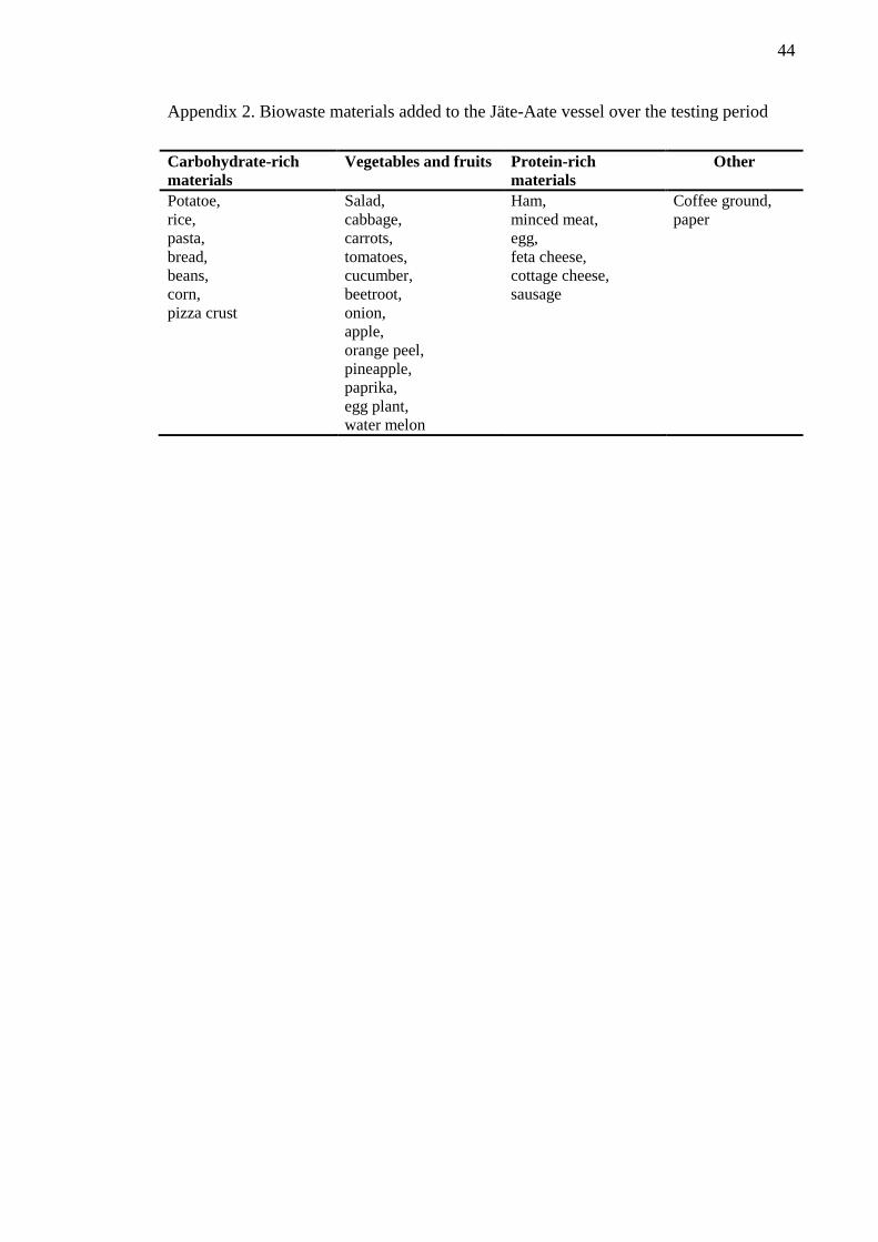
Appendix 2. Biowaste materials added to the Jäte-Aate vessel over the testing period

Carbohydrate-rich

materials

Vegetables and fruits Protein-rich

materials

Other

Potatoe,

rice,

pasta,

bread,

beans,

corn,

pizza crust

Salad,

cabbage,

carrots,

tomatoes,

cucumber,

beetroot,

onion,

apple,

orange peel,

pineapple,

paprika,

egg plant,

water melon

Ham,

minced meat,

egg,

feta cheese,

cottage cheese,

sausage

Coffee ground,

paper

45

Appendix 3. Measurements taken during the testing period (pH, conductivity, CH4,

CO2, O2)

Day Date

pH

conductivity

[mS/cm]

CH4

[%]

CO2

[%]

O2

[%]

17 17.11.2011 3,6 12,71 0,1 44,7 1,7

24 24.11.2011 3,52 13,05 0,1 53,5 0

29 29.11.2011 3,52 13,11 0 57,8 0

31 1.12.2011 3,52 13,05 0 60,2 0

35 5.12.2011 3,52 12,64 0,2 69,6 0

37 7.12.2011 3,45 12,98 - - -

38 8.12.2011 - - 0,1 73,5 0

39 9.12.2011 3,55 12,85 0,1 73,3 0

42 12.12.2011 3,52 12,67 0 43,3 4,2

44 14.12.2011 3,5 12,81 0 40,5 2,5

46 16.12.2011 3,46 12,7 0 38,4 2,1

49 19.12.2011 3,41 12,75 0 56,7 0,9

58 28.12.2011 3,29 - 0 43,4 0,5

65 4.1.2012 3,29 - 0 40,9 0

70 9.1.2012 3,38 12,14 0 36,5 0,3

71 10.1.2012 - - 0 36,1 0,2

72 11.1.2012 3,22 11,89 0 37,6 0,1

74 13.1.2012 3,37 11,28 0 39,5 0,1

77 16.1.2012 3,39 11,83 0 40,3 0

79 18.1.2012 3,38 12,33 0 50,2 0,1

81 20.1.2012 3,38 11,04 0 55,9 0,4

84 23.1.2012 3,38 11,41 0 64,4 0

86 25.1.2012 - 11,66 0,2 67,3 0

88 27.1.2012 3,29 11 0,2 66,9 0,1

92 31.1.2012 3,69 11,69 - - -

46

Appendix 4. Chloride content analysis results of the sample from 24.11.2011

47

48

49

Appendix 5. Chloride content analysis results of the sample from 28.12.2012

50

51

52

Appendix 6. Chloride content analysis results of the sample from 18.1.2012

53

54

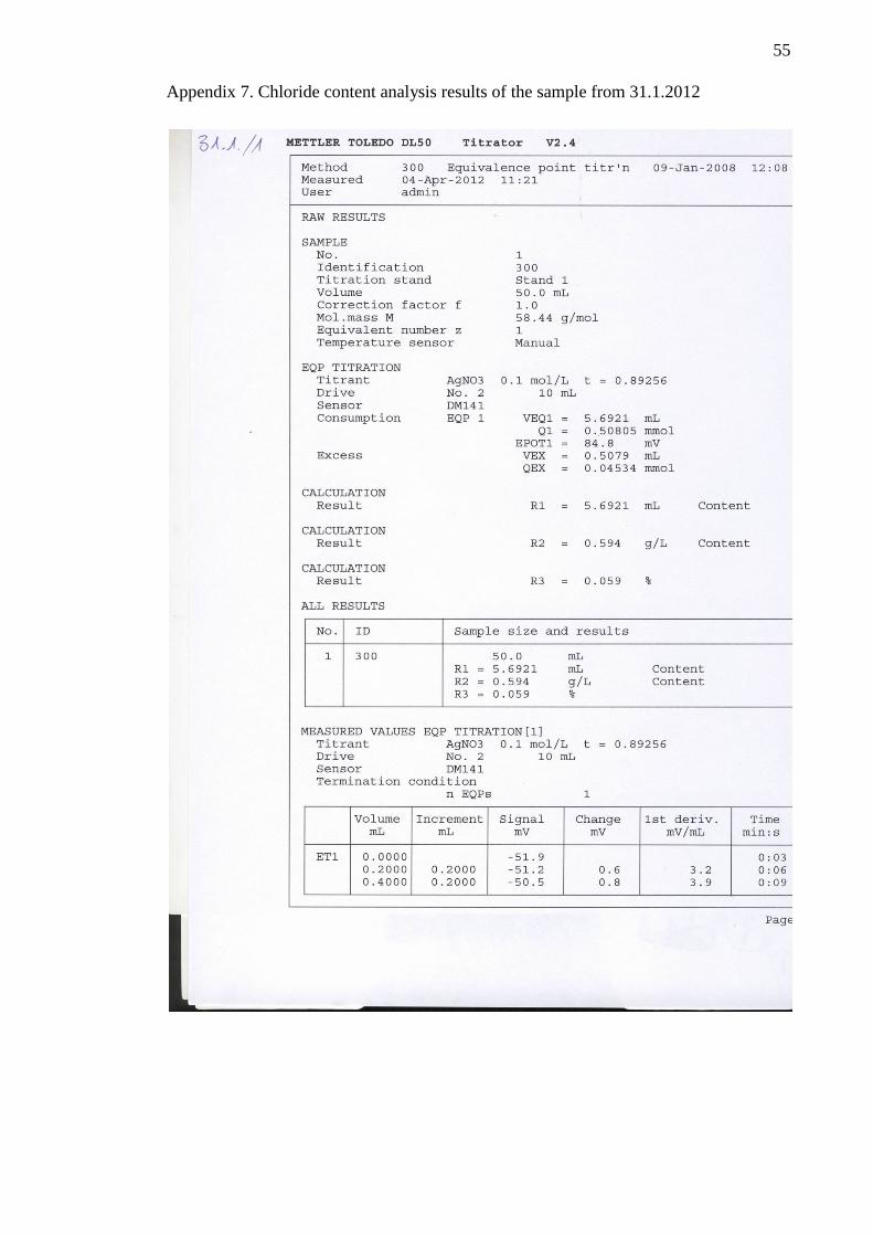
55

Appendix 7. Chloride content analysis results of the sample from 31.1.2012

56

57