Ya’axché Conservation Trust Phone: (+501) 722-0108 22 Alejandro Vernon Street, P.O. 177 Fax: (+501) 722-0108 Punta Gorda, Toledo District E-mail: info@yaaxche.org Belize Web: yaaxche.org

Biodiversity Synthesis Report 2012

Maarten Hofman Research Coordinator

2

Field work conducted by Ya’axché’s ranger team

Anignazio Makin, Indian Creek village Marcus Cholom, Golden Stream village Marcus Tut, Trio village Octavio Cal, Golden Stream village Pastor Ayala, Trio village Rosendo Coy, Indian Creek village Victor Bonilla, Indian Creek village Vigilio Cal, Golden Stream village Zacceus Caal, Golden Stream village

And supervised by

Marchilio Ack – Head ranger Lee McLoughlin – Protected Area Manager

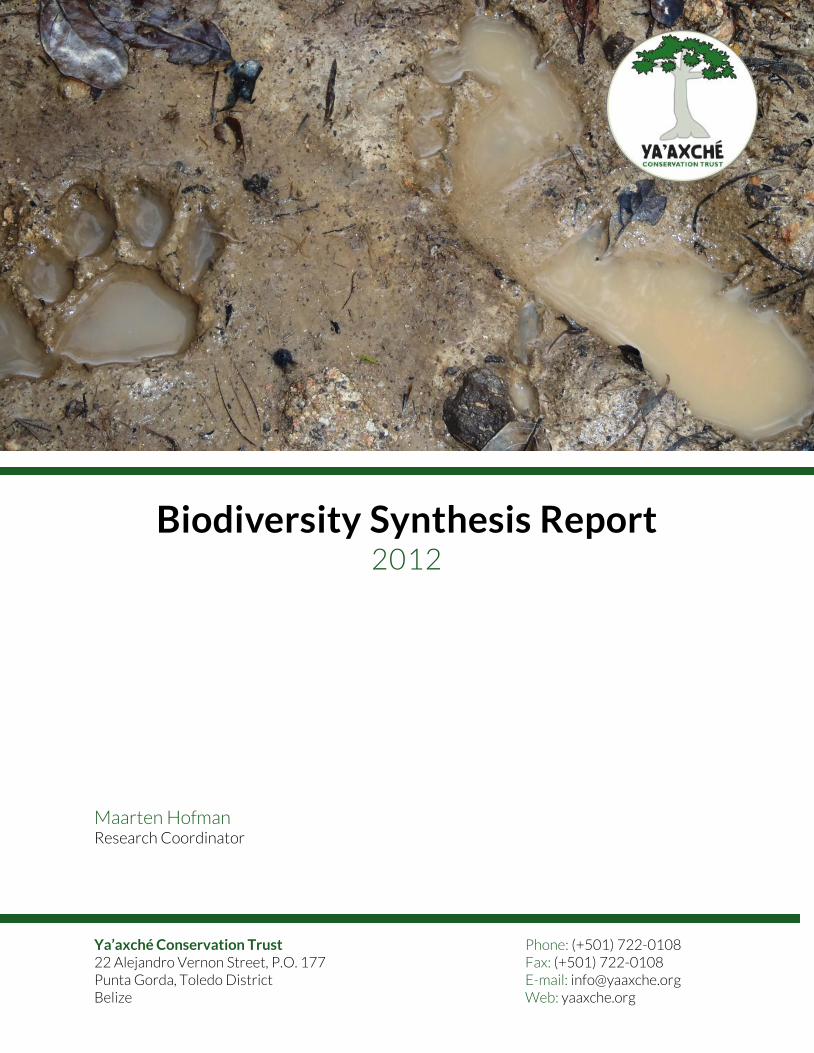
Cover photo: Maarten Hofman © Ya’axché Conservation Trust – November 2013

Citation: Hofman, M., 2013, Biodiversity Synthesis Report - 2012, Ya’axché Conservation Trust, Punta Gorda, Toledo District, Belize.

3

Table of Contents Acronyms .......................................................................................................................................... 4

Summary ........................................................................................................................................... 5

Introduction ..................................................................................................................................... 6

Methodology ................................................................................................................................... 8

Bird and large mammal transects ................................................................................................................ 8

Camera trapping survey ............................................................................................................................... 15

Bats....................................................................................................................................................................... 16

Wildlife observations ..................................................................................................................................... 16

Highway crossings .......................................................................................................................................... 17

Road traffic ........................................................................................................................................................ 17

Land snails.......................................................................................................................................................... 18

Vegetation ......................................................................................................................................................... 19

Weather .............................................................................................................................................................. 19

Fire ....................................................................................................................................................................... 20

Results .............................................................................................................................................. 22

Birds ..................................................................................................................................................................... 22

Large mammals ................................................................................................................................................ 32

Camera trapping.............................................................................................................................................. 40

Bats....................................................................................................................................................................... 42

Wildlife observations ..................................................................................................................................... 43

Highway crossings .......................................................................................................................................... 43

Road traffic ........................................................................................................................................................ 44

Land snails.......................................................................................................................................................... 45

Vegetation ......................................................................................................................................................... 46

Weather .............................................................................................................................................................. 47

Fire ....................................................................................................................................................................... 49

Conclusions .................................................................................................................................... 50

Recommendations ...................................................................................................................... 53

Acknowledgements .................................................................................................................... 55

References ..................................................................................................................................... 56

4

Acronyms

AI Activity Index

AI% Activity Index Percent

BNR Bladen Nature Reserve

BRIM Ya’axché’s Biodiversity Research, Inventory and Monitoring strategy

CRFR Columbia River Forest Reserve

DBH Diameter at breast height

ENS Effective Number of Species (or True Diversity)

GIS Geographical Information System

GSCP Golden Stream Corridor Preserve

MGL Maya Golden Landscape – Ya’axché’s working area

REA Rapid Ecological Assessment

PSP Permanent Sample Plot for vegetation monitoring

Ya’axché Ya’axché Conservation Trust

5

Summary Ya’axché Conservation Trust is a community-orientated NGO that manages the Golden Stream Corridor Preserve (15,000acres) and the Bladen Nature Reserve (100,000acres), located in the southern-most district of Belize, and surrounded by small Mayan villages. This focus area is usually referred to as the Maya Golden Landscape (MGL). Since 2006, Ya’axché has been developing a biodiversity monitoring programme to keep track of the changing environment in the area, and the effects of our conservation actions. The programme initially comprised only transect monitoring for birds and large mammals, and has expanded over the years according to Ya’axché’s Biodiversity Research, Inventory and Monitoring strategy to include freshwater quality, freshwater invertebrates, weather variables, bats, road traffic and wildlife casualties, land use/land cover change, land snails, vegetation and fire patterns. Methods include point, transect and plot sampling in the field, digital data management and digital analysis using GIS, covering the entire MGL. Transect monitoring effort has been doubled since last year, but we didn’t discover more target species for either birds or large mammals. Village lands were less species rich than forested lands and the proportion of forest health indicators gradually decreases as the habitat gets more disturbed. Observations done in the field during patrols and from camera traps show a good abundance and diversity of species, with a tendency towards higher diversity in the less disturbed areas. All five wild cat species, a tamandua hit by traffic and a juvenile harpy eagle were some interesting observations. Bat diversity was much higher in the savannah area than in the forest. The long term trends since 2007 indicate an increase in target species richness and a proportional decrease in number of disturbance indicators. These could be signs of improving habitat quality, but the unknown effect of covariates such as increased skill level and improved monitoring systems might be playing a role here as well. The establishment of six monitoring plots for land snails was fruitful in terms of skills acquired and lessons learnt, but unfortunately yielded data of too low quality to be included. Additional training is required to enable the use of these interesting bio-indicators. From the preliminary analysis of one of two 100x100m vegetation monitoring plots in the Bladen Nature Reserve, we confirm that the area has one of the highest number of tree species in all of Central America. Once the weather monitoring efforts (both manual and automated stations) have stabilised, the relation between weather patterns and escaped fires could be investigated and used in Ya’axché outreach activities to reduce deforestation by escaped fires. With the data gathered over the last 6 years, we have established a baseline for many useful indicators, and we have confirmed Ya’axché’s ability to maintain and develop a biodiversity monitoring programme. However, we are aware that such a programme is never really completed, and we will continue to build and improve it according to national and international guidelines.

6

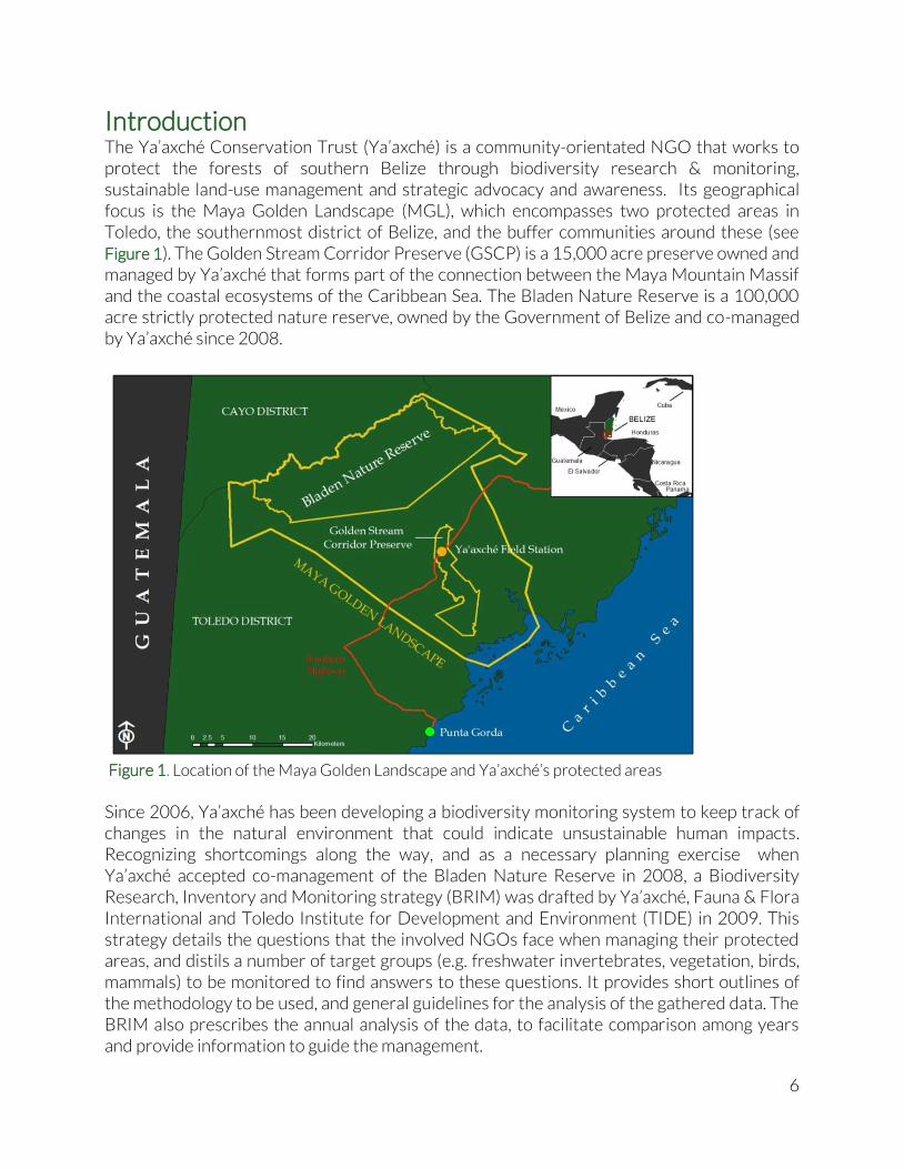
Introduction The Ya’axché Conservation Trust (Ya’axché) is a community-orientated NGO that works to protect the forests of southern Belize through biodiversity research & monitoring, sustainable land-use management and strategic advocacy and awareness. Its geographical focus is the Maya Golden Landscape (MGL), which encompasses two protected areas in Toledo, the southernmost district of Belize, and the buffer communities around these (see Figure 1). The Golden Stream Corridor Preserve (GSCP) is a 15,000 acre preserve owned and managed by Ya’axché that forms part of the connection between the Maya Mountain Massif and the coastal ecosystems of the Caribbean Sea. The Bladen Nature Reserve is a 100,000 acre strictly protected nature reserve, owned by the Government of Belize and co-managed by Ya’axché since 2008.

Since 2006, Ya’axché has been developing a biodiversity monitoring system to keep track of changes in the natural environment that could indicate unsustainable human impacts. Recognizing shortcomings along the way, and as a necessary planning exercise when Ya’axché accepted co-management of the Bladen Nature Reserve in 2008, a Biodiversity Research, Inventory and Monitoring strategy (BRIM) was drafted by Ya’axché, Fauna & Flora International and Toledo Institute for Development and Environment (TIDE) in 2009. This strategy details the questions that the involved NGOs face when managing their protected areas, and distils a number of target groups (e.g. freshwater invertebrates, vegetation, birds, mammals) to be monitored to find answers to these questions. It provides short outlines of the methodology to be used, and general guidelines for the analysis of the gathered data. The BRIM also prescribes the annual analysis of the data, to facilitate comparison among years and provide information to guide the management.

Figure 1. Location of the Maya Golden Landscape and Ya’axché’s protected areas

7

Ya’axché has collected data on birds and large mammals using transect monitoring throughout the Maya Golden Landscape since 2006. From 2009 onwards, the ranger team got trained in freshwater invertebrate sampling and freshwater quality monitoring by Ya’axché’s freshwater ecologist, Rachael Carrie, who also initiated the weather monitoring activities. In 2011, bats were added to the monitoring programme after a multi-day training session in species diversity, field methods and data handling by Dr. Bruce Miller. This year, 2012, has seen a considerable number of additions as well. A land snail monitoring component was added after training by snail specialists Dan Dourson and Dr. Ron Caldwell. The appointment of a volunteer botanist, Gail Stott, in January 2011 and subsequent collaboration with plant ecology consultant Dr. Steven Brewer has enabled Ya’axché to add vegetation monitoring to the existing programme by establishing two one-hectare Permanent Sample Plots (PSPs) according to international standards. Also in 2012, we established a baseline of road traffic density in the frames of GSCP’s corridor function, and continued collecting anecdotal evidence of highway crossings and casualties. And last but not least, the involvement of a GIS specialist volunteer, Jaume Ruscalleda, has increased Ya’axché’s capacity to use remote sensing and satellite imagery to monitor land use and land cover change (Ruscalleda 2011; Ruscalleda 2012) and fire (this report). Fire plays an important role in the lives of people in southern Belize. It is regarded as a necessity for successful farming, is used as a hunting technique and to clear vegetation from roadsides. Many people start a fire for these reasons, but are ill-equipped and lack the fire management knowledge to control the fire they started. Escaping fires are therefore one of the main threats to forest and biodiversity conservation in the area. With the inclusion of fire monitoring and the (re)instalment of transects on village lands and in the savannah, we have made a first move towards a more inclusive landscape-scale monitoring approach. It is clear that the Biodiversity Research, Inventory and Monitoring programme has acquired components that cannot strictly be categorised as ‘biodiversity’, such as freshwater quality, weather, fire and road traffic monitoring. However, for the time being, we consider these components too limited to warrant a change in the concept of our annual reporting scheme. The 2010 Biodiversity Synthesis Report (Hofman 2012) was a first step towards the fulfilment of the BRIM requirement to report the findings annually. The 2011 report (Hofman et al. 2013) built on this to form a more complete biodiversity report, including the bat monitoring results and weather data. The 2012 report includes a report on the extent of fires in the Maya Golden Landscape, and an improved presentation of the transect monitoring data. Importantly, for this report we have also reanalysed the transect monitoring data from all previous years back to 2007and put the results of these next to the information from the Annual Biodiversity Synthesis Reports for a basic trend analysis. Besides recording and illustrating the development of the monitoring programme at Ya’axché over the years, this is ultimately the goal of these reports: to enable comparison of biodiversity among years and with the results inform Ya’axché’s strategies with regards to protected areas management and community development.

8

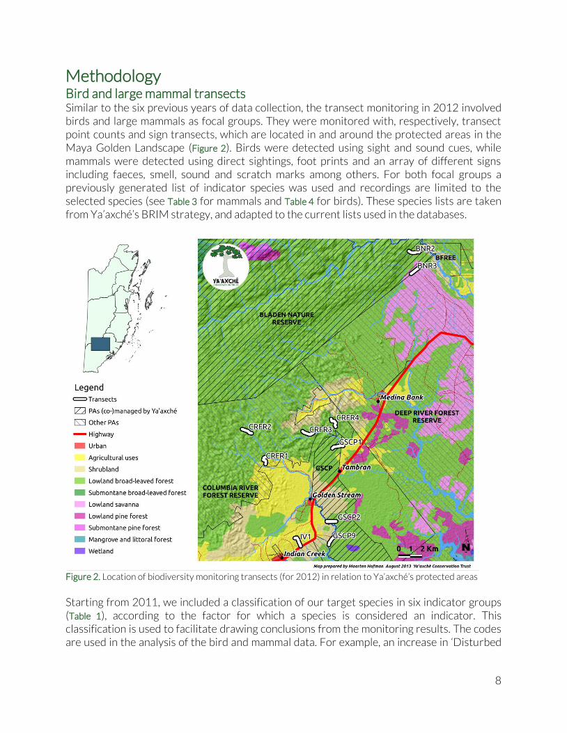
Methodology Bird and large mammal transects Similar to the six previous years of data collection, the transect monitoring in 2012 involved birds and large mammals as focal groups. They were monitored with, respectively, transect point counts and sign transects, which are located in and around the protected areas in the Maya Golden Landscape (Figure 2). Birds were detected using sight and sound cues, while mammals were detected using direct sightings, foot prints and an array of different signs including faeces, smell, sound and scratch marks among others. For both focal groups a previously generated list of indicator species was used and recordings are limited to the selected species (see Table 3 for mammals and Table 4 for birds). These species lists are taken from Ya’axché’s BRIM strategy, and adapted to the current lists used in the databases.

Figure 2. Location of biodiversity monitoring transects (for 2012) in relation to Ya’axché’s protected areas

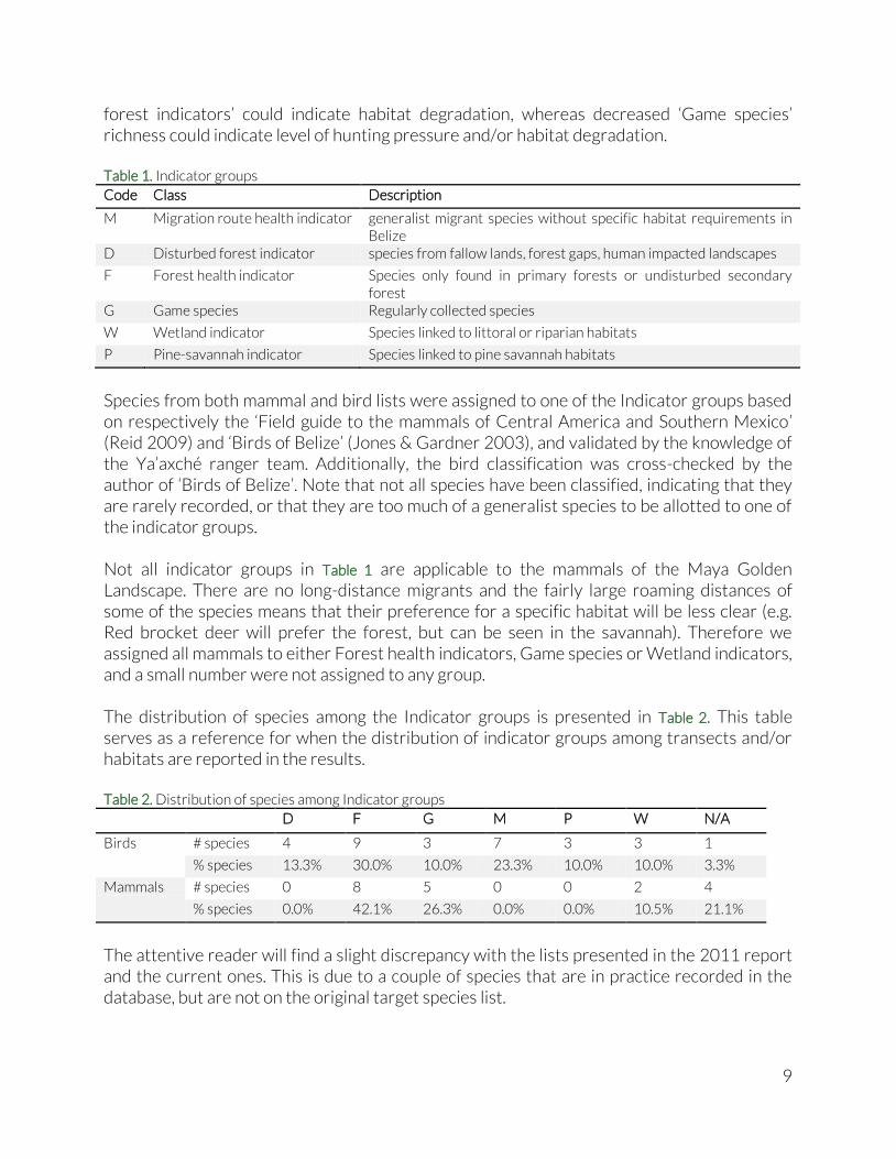
Starting from 2011, we included a classification of our target species in six indicator groups (Table 1), according to the factor for which a species is considered an indicator. This classification is used to facilitate drawing conclusions from the monitoring results. The codes are used in the analysis of the bird and mammal data. For example, an increase in ‘Disturbed

9

forest indicators’ could indicate habitat degradation, whereas decreased ‘Game species’ richness could indicate level of hunting pressure and/or habitat degradation. Table 1. Indicator groups

Code Class Description

M Migration route health indicator generalist migrant species without specific habitat requirements in Belize

D Disturbed forest indicator species from fallow lands, forest gaps, human impacted landscapes

F Forest health indicator Species only found in primary forests or undisturbed secondary forest

G Game species Regularly collected species

W Wetland indicator Species linked to littoral or riparian habitats

P Pine-savannah indicator Species linked to pine savannah habitats

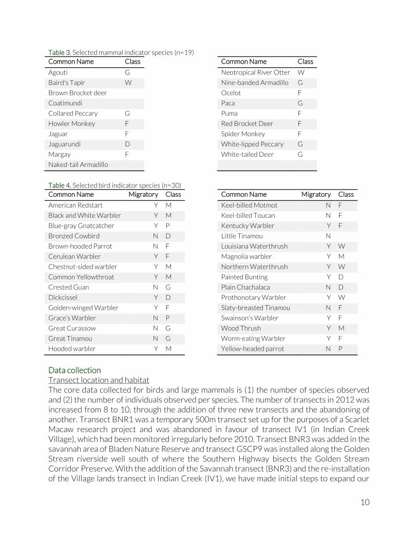
Species from both mammal and bird lists were assigned to one of the Indicator groups based on respectively the ‘Field guide to the mammals of Central America and Southern Mexico’ (Reid 2009) and ‘Birds of Belize’ (Jones & Gardner 2003), and validated by the knowledge of the Ya’axché ranger team. Additionally, the bird classification was cross-checked by the author of ‘Birds of Belize’. Note that not all species have been classified, indicating that they are rarely recorded, or that they are too much of a generalist species to be allotted to one of the indicator groups. Not all indicator groups in Table 1 are applicable to the mammals of the Maya Golden Landscape. There are no long-distance migrants and the fairly large roaming distances of some of the species means that their preference for a specific habitat will be less clear (e.g. Red brocket deer will prefer the forest, but can be seen in the savannah). Therefore we assigned all mammals to either Forest health indicators, Game species or Wetland indicators, and a small number were not assigned to any group. The distribution of species among the Indicator groups is presented in Table 2. This table serves as a reference for when the distribution of indicator groups among transects and/or habitats are reported in the results. Table 2. Distribution of species among Indicator groups

D F G M P W N/A

Birds # species 4 9 3 7 3 3 1

% species 13.3% 30.0% 10.0% 23.3% 10.0% 10.0% 3.3%

Mammals # species 0 8 5 0 0 2 4

% species 0.0% 42.1% 26.3% 0.0% 0.0% 10.5% 21.1%

The attentive reader will find a slight discrepancy with the lists presented in the 2011 report and the current ones. This is due to a couple of species that are in practice recorded in the database, but are not on the original target species list.

10

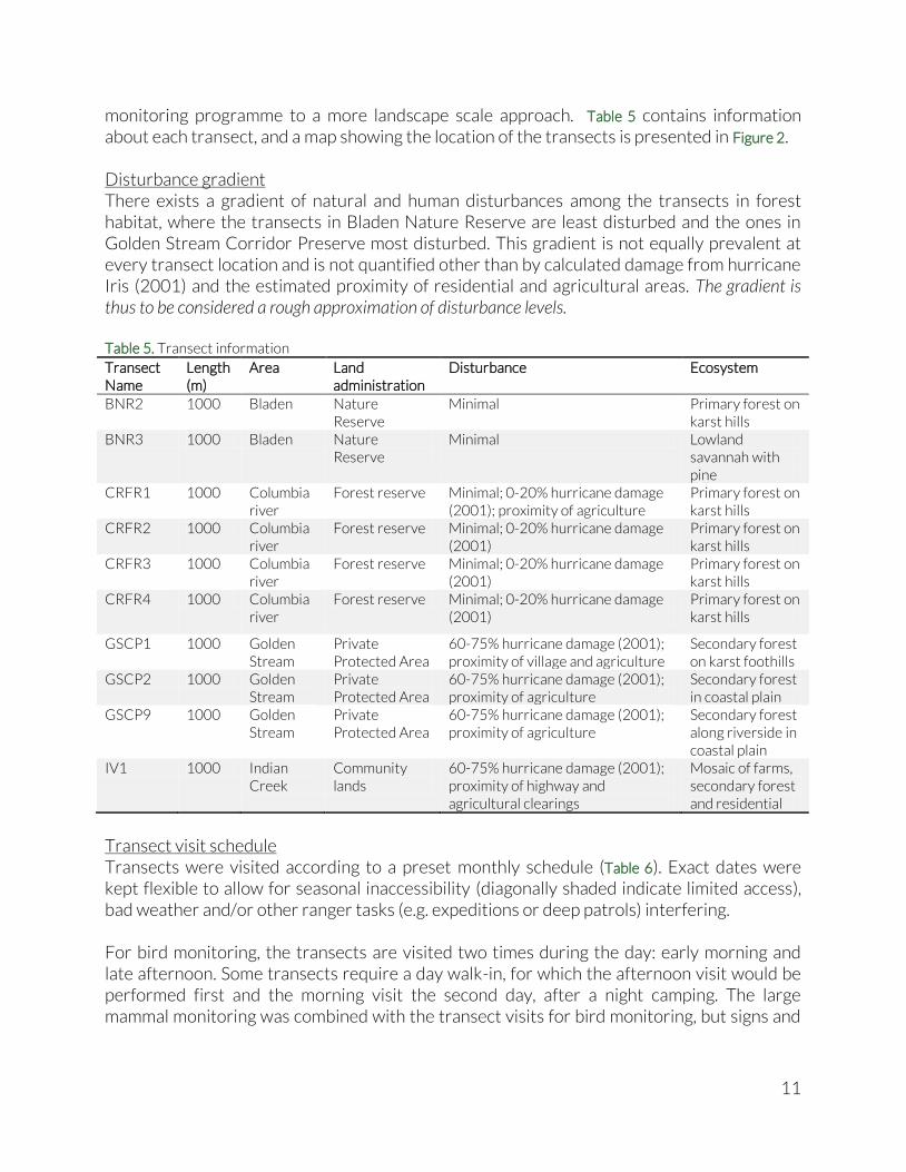
Table 3. Selected mammal indicator species (n=19)

Common Name Class

Agouti G

Baird's Tapir W

Brown Brocket deer

Coatimundi

Collared Peccary G

Howler Monkey F

Jaguar F

Jaguarundi D

Margay F

Naked-tail Armadillo

Common Name Class

Neotropical River Otter W

Nine-banded Armadillo G

Ocelot F

Paca G

Puma F

Red Brocket Deer F

Spider Monkey F

White-lipped Peccary G

White-tailed Deer G

Table 4. Selected bird indicator species (n=30)

Common Name Migratory Class

American Redstart Y M

Black and White Warbler Y M

Blue-gray Gnatcatcher Y P

Bronzed Cowbird N D

Brown-hooded Parrot N F

Cerulean Warbler Y F

Chestnut-sided warbler Y M

Common Yellowthroat Y M

Crested Guan N G

Dickcissel Y D

Golden-winged Warbler Y F

Grace’s Warbler N P

Great Curassow N G

Great Tinamou N G

Hooded warbler Y M

Common Name Migratory Class

Keel-billed Motmot N F

Keel-billed Toucan N F

Kentucky Warbler Y F

Little Tinamou N

Louisiana Waterthrush Y W

Magnolia warbler Y M

Northern Waterthrush Y W

Painted Bunting Y D

Plain Chachalaca N D

Prothonotary Warbler Y W

Slaty-breasted Tinamou N F

Swainson’s Warbler Y F

Wood Thrush Y M

Worm-eating Warbler Y F

Yellow-headed parrot N P

Data collection Transect location and habitat The core data collected for birds and large mammals is (1) the number of species observed and (2) the number of individuals observed per species. The number of transects in 2012 was increased from 8 to 10, through the addition of three new transects and the abandoning of another. Transect BNR1 was a temporary 500m transect set up for the purposes of a Scarlet Macaw research project and was abandoned in favour of transect IV1 (in Indian Creek Village), which had been monitored irregularly before 2010. Transect BNR3 was added in the savannah area of Bladen Nature Reserve and transect GSCP9 was installed along the Golden Stream riverside well south of where the Southern Highway bisects the Golden Stream Corridor Preserve. With the addition of the Savannah transect (BNR3) and the re-installation of the Village lands transect in Indian Creek (IV1), we have made initial steps to expand our

11

monitoring programme to a more landscape scale approach. Table 5 contains information about each transect, and a map showing the location of the transects is presented in Figure 2. Disturbance gradient There exists a gradient of natural and human disturbances among the transects in forest habitat, where the transects in Bladen Nature Reserve are least disturbed and the ones in Golden Stream Corridor Preserve most disturbed. This gradient is not equally prevalent at every transect location and is not quantified other than by calculated damage from hurricane Iris (2001) and the estimated proximity of residential and agricultural areas. The gradient is thus to be considered a rough approximation of disturbance levels. Table 5. Transect information

Transect Name

Length (m)

Area Land administration

Disturbance Ecosystem

BNR2 1000 Bladen Nature Reserve

Minimal Primary forest on karst hills

BNR3 1000 Bladen Nature Reserve

Minimal Lowland savannah with pine

CRFR1 1000 Columbia river

Forest reserve Minimal; 0-20% hurricane damage (2001); proximity of agriculture

Primary forest on karst hills

CRFR2 1000 Columbia river

Forest reserve Minimal; 0-20% hurricane damage (2001)

Primary forest on karst hills

CRFR3 1000 Columbia river

Forest reserve Minimal; 0-20% hurricane damage (2001)

Primary forest on karst hills

CRFR4 1000 Columbia river

Forest reserve Minimal; 0-20% hurricane damage (2001)

Primary forest on karst hills

GSCP1 1000 Golden Stream

Private Protected Area

60-75% hurricane damage (2001); proximity of village and agriculture

Secondary forest on karst foothills

GSCP2 1000 Golden Stream

Private Protected Area

60-75% hurricane damage (2001); proximity of agriculture

Secondary forest in coastal plain

GSCP9 1000 Golden Stream

Private Protected Area

60-75% hurricane damage (2001); proximity of agriculture

Secondary forest along riverside in coastal plain

IV1 1000 Indian Creek

Community lands

60-75% hurricane damage (2001); proximity of highway and agricultural clearings

Mosaic of farms, secondary forest and residential

Transect visit schedule Transects were visited according to a preset monthly schedule (Table 6). Exact dates were kept flexible to allow for seasonal inaccessibility (diagonally shaded indicate limited access), bad weather and/or other ranger tasks (e.g. expeditions or deep patrols) interfering. For bird monitoring, the transects are visited two times during the day: early morning and late afternoon. Some transects require a day walk-in, for which the afternoon visit would be performed first and the morning visit the second day, after a night camping. The large mammal monitoring was combined with the transect visits for bird monitoring, but signs and

12

sightings were only recorded during either the morning or the evening visit. A more detailed description of the methodology used on the transects can be found in the BRIM. Table 6. Transect visit schedule 2012; shaded areas indicate periodic inaccessibility

Month BNR 2 BNR 3 GSCP 1 GSCP 2 GSCP9 CRFR 1 CRFR 2 CRFR 3 CRFR 4 IV1 Total

Dry

se

aso

n Jan 1 1 1 1 1 1 1 7

Feb 1 1 1 1 1 1 6 Mar 1 1 1 1 1 1 1 7 Apr 1 1 1 1 1 1 6 May 1 1 1 1 1 1 1 7

We

t se

aso

n

Jun 1 1 1 1 1 1 6 Jul 1 1 1 1 1 1 1 7 Aug 1 1 1 1 1 1 6 Sep 1 1 1 1 1 1 1 7 Oct 1 1 1 1 1 1 6 Nov 1 1 1 1 1 1 1 7

Dec 1 1 1 1 1 1 6

Total 12 12 6 6 6 6 6 6 6 12 78

Data quality The quality of the data collected on transects and the way it is entered in the database has significantly improved since the first Biodiversity Synthesis Report was produced for 2010 (Hofman 2012). Putting the transect visit schedule in place, and prioritizing over other activities, has doubled the visit frequency and the number of individuals observed, despite a dent in efficiency by the end of the year (see Figure 5 on p23). Additional training sessions were held for the ranger team to refresh and improve field monitoring techniques, which increased the level of accuracy and detail of their recorded data. Training sessions to enhance data entry skills in both spreadsheet and database environments has enabled the improved field recording to be reflected in more consistent and correct databases. Data inconsistencies such as observations without species name or number of individuals observed are virtually eliminated from the database. No observations lacked species name for birds and mammals, and the 9 observations that lacked number of individuals in the mammal data were set conservatively to ‘1’. Data analysis The data analyses uses the instructions in the BRIM as a starting point, but were mostly built on the progress accomplished over the last two Biodiversity Synthesis Reports (Hofman 2012; Hofman et al. 2013). Most analyses were done per transect, thereby pooling together the data from all visits for each transect. This was considered a suitable way to achieve a good overview of larger scale differences between transects. With the addition of two transects outside forested habitats, we have included a comparison of indicator groups between the forest, savannah and community lands habitat, which gives us more of a landscape level perspective.

13

Actual number of observed species (Target Species Richness) The actual number of species observed is the raw biodiversity data that is a sample of the total actual biodiversity of the ecosystems. It was calculated for every transect based on all species for which at least one individual was observed, on any of the visits to that transect. It needs to be stressed that the species richness has an upper limit equal to the number of target species on the lists mentioned above (see Table 3 and Table 4), hence the name Target Species Richness. Diversity profiles Contrary to the previous Biodiversity Synthesis Reports, we will not go into detail on the relative abundances, the individual diversity indices and the Effective Number of Species per transect. Instead, we will combine all these components in an approach called Diversity profiles (Tóthmérész 1995; Magurran 2004; Hill & Mar 1973). The diversity profiles will inform us in an integrated fashion about the species diversity among different transects and the effects of dominance. A diversity profile of a transect is in fact a more elaborate version of the Hill series graphs presented in the 2011 Biodiversity Synthesis Report (Hofman et al. 2013); they visualise the Effective Number of Species calculated from the different diversity indices (Target species richness [R], Shannon’s index [H] and Simpson’s index [λ]). In fact, these three diversity measures reflect the same diversity, but, to estimate the Effective Number of Species, they weigh species differently according to their relative abundance (i.e. rarity or dominance). Target species richness counts every species equally, no matter how few times it was detected, and thus doesn’t take into account the relative abundance. Shannon’s index weighs every species according to its relative abundance, making the rarest species contribute less to the Effective Number of Species estimate. Simpsons index goes further and gives proportionately more weight to those species with the highest relative abundance, hence amplifying the dominance of certain species. This gradient is called the ‘order’ of diversity, and is captured using a scaling factor (α), derived from Rényi’s entropy (Rényi 1961):

Where Dα represents the species diversity of order α, pi indicates the relative abundance of species i, and S stands for the total number of species. When α equals zero, we obtain the Target species richness. When α equals 1, we obtain the Effective Number of Species that corresponds to the exponential of the Shannon’s index (eH). And when α equals 2, we get the Effective Number of Species that is equivalent to the inverse of Simpon’s index. If we plot the Effective Number of Species as a function of the value of α, we obtain a diversity profile, which enables us to detect both species richness and dominance effect (or ‘evenness’ of relative species abundance) at the same time. The higher the profile, the higher the diversity. If two diversity profiles cross, the communities have different levels of dominance and are said to be non-comparable

14

(Tóthmérész 1995; Jost 2010). The diversity profiles were plotted using the PASTv2.17c software (Hammer et al. 2001). Species accumulation curves and rarefaction curves Importantly, since not all transects have an equal number of transect visits, abundance data cannot be interpreted easily. Transects that have been visited once or twice, cannot possibly have uncovered the same number of species than transects that have been visited four times or more. To provide comparison with the 2011 Biodiversity Synthesis Report, we present a species accumulation curve show the cumulative increase of detected species on a transect as subsequent visits are performed. The presented curves display the average species accumulation across all transects. Species accumulation curves are sometimes used to predict the total number of species in a certain area using so-called species-area relationship. However, there are two reasons why this is not a fruitful approach in our case. First, our transect methods do not include recording of detection distance, which means that we cannot calculate the surface area in which the species were detected. Second, because we are working with a fixed set of target species, the accumulation has an inherent asymptote (e.g. 30 species for our bird list). Any prediction of total species richness for the area would thus be impossible. Therefore, instead of predicting the total species richness of each transect, we use rarefaction curves (Gotelli & Colwell 2001; Magurran 2004) that allow us to compare species accumulation between transects: which transect has accumulated most species after a set number of transect visits? Usually, this set number of transect visits is determined by the transect with the least visits. Rarefaction curves are created by repeatedly drawing a random subset of transect visits from one transect (with varying number of visits per draw), registering the species richness per draw, and then plotting the average number of species found as a function of the number of transect visits. Thus rarefaction generates the expected number of species in a small collection of transect visits drawn at random from the large pool of transect visits of that transect. The rarefaction curves were calculated and plotted using the PASTv2.17c software (Hammer et al. 2001). Indicator Groups To gauge the effects of habitat disturbance on the species composition, we sum up all individual birds observed and calculate the percentage that fall in each Indicator Group. We use percentages to standardize visit frequency and number of species across transects. We compare between transects, between habitat and between years. Trends in the forests of the Maya Golden Landscape To compare long term trends, we made use of transect data that was gathered from 2007 onwards (see Table 7). The methodologies used for the transect monitoring have remained the same for this entire period, however monitoring intensity has varied (number of transects, number of transect visits and number of target species). Some transects have been monitored since 2007, others were established as late as 2012. Some transects on village lands have been abandoned and haven’t been visited since 2009 due to a shift in community relations. Additionally, over the last three years (2010-2012) the data recording systems

15

have been improved significantly and training in data gathering techniques as well as data entering has increased the skill level of all rangers considerably. During the same period, the supervision over the data gathering and entry was improved, again increasing data quality. All of these factors were not quantified and thus cannot be controlled for. They can have a big impact on the direct comparison among years.

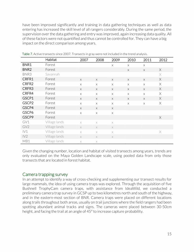
Given the changing number, location and habitat of visited transects among years, trends are only evaluated on the Maya Golden Landscape scale, using pooled data from only those transects that are located in forest habitat.

Camera trapping survey In an attempt to identify a way of cross-checking and supplementing our transect results for large mammals, the idea of using camera traps was explored. Through the acquisition of five Bushnell TrophyCam camera traps, with assistance from IdeaWild, we conducted a preliminary camera trap survey in GCSP up to two kilometres north and south of the highway, and in the eastern-most section of BNR. Camera traps were placed on different locations along trails throughout both areas, usually on trail junctions where the field rangers had been spotting abundant animal tracks and signs. The cameras were placed between 30-50cm height, and facing the trail at an angle of 45° to increase capture probability.

Habitat 2007 2008 2009 2010 2011 2012

BNR1 Forest

x x x

BNR2 Forest

x x X

BNR3 Savannah

X

CRFR1 Forest x x x x x X

CRFR2 Forest x x x x x X

CRFR3 Forest x x x x x X

CRFR4 Forest x x x x x X

GSCP1 Forest x x x x x X

GSCP2 Forest x x x x x X

GSCP4 Forest x x x

GSCP6 Forest x x x

GSCP9 Forest

X

GV1 Village lands x x x

GV2 Village lands x x x

IV1 Village lands x x x

X

IV2 Village lands x x x

MB1 Village lands x x

Table 7. Active transects since 2007. Transects in gray were not included in the trend analysis.

16

Bats As a follow-up to the opportunistic bat monitoring during 2011, a more systematic approach was envisioned for 2012, aiming to use the transect visit schedule to achieve a pre-set visit frequency. The single passive acoustic monitoring station, comprised of an Anabat detector, a CF-ZCAIM recorder (Titley Scientific, Brisbane, Australia) and remotely mounted microphone was taken on several visits of the bird and large mammal transects throughout the year according to the transect schedule. The unit was pre-programmed with a beginning and ending recording time to approximately coincide with sunset and sunrise. The unit records the species-specific ultra-sound echolocation calls, which are visualised and cross-checked with an existing database of species calls to identify to species level. This is done by Dr. Bruce Miller who reported the number of species detected, species names and their associated Acoustic Activity Index (AI). The Acoustic Activity Index was developed by Miller (2001) as an index of relative abundance and is calculated as

where p stands for any given one-minute time block during which the species was present (i.e. detected at least once). Dividing by the unit effort for the survey standardizes the AI. In this case, the AI (number of one-minute time blocks) was divided by the total survey time at that sample location, to obtain the proportion of one-minute time blocks that a bat species was active during the sample period. Subsequent nights surveyed at one location were treated as a single sample. Hence we obtain a relative version of the AI, which we have termed the Activity Index Percent (AI%):

where P is the total number of one-minute time blocks in the sample.

Wildlife observations As an addition to the systematic biodiversity monitoring of large mammals and birds, Ya’axché rangers also recorded noteworthy observations made while patrolling the protected areas. Only actual sightings of animals are recorded. Tracks and other signs are ignored. Even though daily patrols are conducted in both GSCP and BNR, their target area and length is tailored to enforcement needs and thus very irregular and unpredictable. Therefore no standardised indices can be derived from the observations. They merely serve as an informal indicator of presence and abundance of wildlife species in the area. Patrols done in BNR sometimes leave from the Golden Stream field center and cross the Columbia River Forest Reserve. A small number of sightings done in CRFR were categorised under BNR.

17

Highway crossings In the frames of the corridor function of Ya’axché’s protected areas, more specifically the Golden Stream Corridor Preserve, opportunistic data was collected on wildlife crossings and casualties along the Southern Highway, and specifically the stretch between the villages of Big Falls and Medina Bank. Data was collected during the daily commute by Ya’axché rangers and other staff between their homes and the field center in the Golden Stream Corridor Preserve. Every 10 days, the staff was asked to report any remarkable road crossings or casualties. Species name, number of individuals and crossing direction (if known) were recorded, as well as the approximate location along the highway.

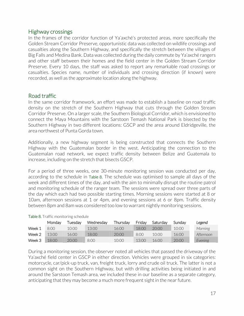
Road traffic In the same corridor framework, an effort was made to establish a baseline on road traffic density on the stretch of the Southern Highway that cuts through the Golden Stream Corridor Preserve. On a larger scale, the Southern Biological Corridor, which is envisioned to connect the Maya Mountains with the Sarstoon Temash National Park is bisected by the Southern Highway in two different locations: GSCP and the area around Eldridgeville, the area northwest of Punta Gorda town. Additionally, a new highway segment is being constructed that connects the Southern Highway with the Guatemalan border in the west. Anticipating the connection to the Guatemalan road network, we expect traffic density between Belize and Guatemala to increase, including on the stretch that bisects GSCP. For a period of three weeks, one 30-minute monitoring session was conducted per day, according to the schedule in Table 8. The schedule was optimised to sample all days of the week and different times of the day, and with the aim to minimally disrupt the routine patrol and monitoring schedule of the ranger team. The sessions were spread over three parts of the day which each had two possible starting times. Morning sessions were started at 8 or 10am, afternoon sessions at 1 or 4pm, and evening sessions at 6 or 8pm. Traffic density between 8pm and 8am was considered too low to warrant nightly monitoring sessions. Table 8. Traffic monitoring schedule

Monday Tuesday Wednesday Thursday Friday Saturday Sunday

Legend

Week 1 8:00 10:00 13:00 16:00 18:00 20:00 10:00

Morning

Week 2 13:00 16:00 18:00 20:00 8:00 10:00 16:00

Afternoon

Week 3 18:00 20:00 8:00 10:00 13:00 16:00 20:00

Evening

During a monitoring session, the observer noted all vehicles that passed the driveway of the Ya’axché field center in GSCP in either direction. Vehicles were grouped in six categories: motorcycle, car/pick-up truck, van, freight truck, lorry and crude oil truck. The latter is not a common sight on the Southern Highway, but with drilling activities being initiated in and around the Sarstoon Temash area, we included these in our baseline as a separate category, anticipating that they may become a much more frequent sight in the near future.

18

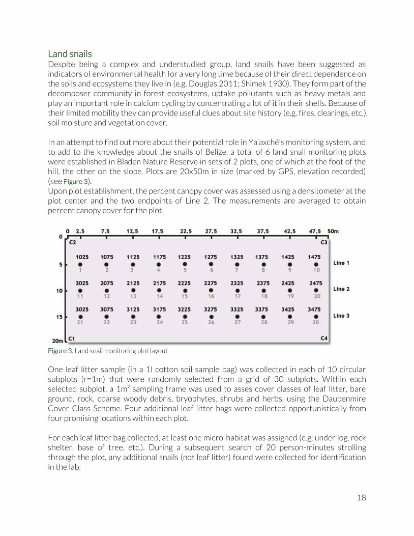
Land snails Despite being a complex and understudied group, land snails have been suggested as indicators of environmental health for a very long time because of their direct dependence on the soils and ecosystems they live in (e.g. Douglas 2011; Shimek 1930). They form part of the decomposer community in forest ecosystems, uptake pollutants such as heavy metals and play an important role in calcium cycling by concentrating a lot of it in their shells. Because of their limited mobility they can provide useful clues about site history (e.g. fires, clearings, etc.), soil moisture and vegetation cover. In an attempt to find out more about their potential role in Ya’axché’s monitoring system, and to add to the knowledge about the snails of Belize, a total of 6 land snail monitoring plots were established in Bladen Nature Reserve in sets of 2 plots, one of which at the foot of the hill, the other on the slope. Plots are 20x50m in size (marked by GPS, elevation recorded) (see Figure 3). Upon plot establishment, the percent canopy cover was assessed using a densitometer at the plot center and the two endpoints of Line 2. The measurements are averaged to obtain percent canopy cover for the plot.

Figure 3. Land snail monitoring plot layout

One leaf litter sample (in a 1l cotton soil sample bag) was collected in each of 10 circular subplots (r=1m) that were randomly selected from a grid of 30 subplots. Within each selected subplot, a 1m² sampling frame was used to asses cover classes of leaf litter, bare ground, rock, coarse woody debris, bryophytes, shrubs and herbs, using the Daubenmire Cover Class Scheme. Four additional leaf litter bags were collected opportunistically from four promising locations within each plot. For each leaf litter bag collected, at least one micro-habitat was assigned (e.g. under log, rock shelter, base of tree, etc.). During a subsequent search of 20 person-minutes strolling through the plot, any additional snails (not leaf litter) found were collected for identification in the lab.

19

Upon arrival in the lab, the leaf litter bags were stored in a dry place to be processed. The snails were separated to the finest taxonomic level achievable, stored in a vial with the subplot info included, and entered in an excel data sheet. After processing a leaf litter bag, a small portion of the leaf litter was put aside and was sent to Dr. Adam W. Rollins, Assistant Professor at Lincoln Memorial University, for his investigations on myxogastrids (slime molds).

Vegetation Plot locations were determined by Dr. Brewer based on existing information on topography, habitats and elevation. Two one-hectare (100 m x 100 m) permanent plots were established: the first on a limestone slope and the second on a limestone ridge. They were installed during the 2012 dry season following a standardized methodology used throughout the tropics (Condit 1998). PVC posts (at 10 m and 20 m intervals) were used to mark out grid of 25 quadrats within the plot. All nine Ya’axché field rangers were involved in the process, some being trained in plot demarcation, others assisting with identification of trees, and with collection of plant material for identification purposes. In both plots, all stems with a diameter at breast height (DBH – measured at 1.3 m) of 5cm or more were recorded and tagged using pre-numbered aluminium tags, and were then identified to species. Where identification of taxa in the field was not possible, voucher specimens (3 sets) were collected and species determinations were made by Dr. Brewer at a later date by comparing collected material with specimens held at the herbarium of Missouri Botanical Gardens, USA. Field identification of stems in the slope plot was completed in April 2013 with only a small number of voucher specimens still to be determined at the time of writing. Field identification of stems (c. 3000) in the ridge plot will be completed by end February 2014. Plot and collections data have been entered into a database. Physical and compositional structure of plot data will be analyzed by end June 2014. This will include a comparison with two existing PSP’s in BNR (established by Dr. Brewer in 1996).

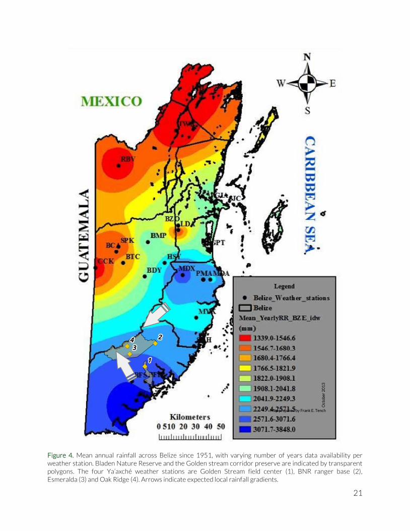
Weather Belize’s weather is characterised by a rainfall gradient that increases roughly from north to south (see Figure 4). Long-term rainfall data are yearly averages and the countrywide coverage is extrapolated from a set of several weather stations distributed over the country, with a limited set of stations in the southern part of the country. More detailed weather information would enable a more localised picture of specific circumstances that might inform us about for example farming success or failure in certain years. Therefore we gather rainfall data, temperature and relative humidity data at the two Ya’axché ranger bases located at Golden Stream Corridor Preserve (W088°47'13.90" N16°22'23.41" [WGS 84]) and Bladen Nature Reserve (W088°42'44.79" N16°32'07.61"

20

[WGS 84]). The weather station in Golden Stream Corridor Preserve was composed of an electronic temperature and humidity device (Digital Hygro-Thermometer, Forestry Suppliers Inc.), and a manually operated rain gauge. At the Bladen Nature Reserve ranger base, only a manually operated rain gauge was available. Data was recorded manually and entered in a spreadsheet. In addition to the two manually operated weather stations, two fully automated weather stations were deployed in Bladen Nature Reserve in 2012. The systems consist of four sensors that measure rainfall, wind speed, temperature, relative humidity and Photosynthetically Active Radiation (sunlight), and are attached to a data logger which stores measurements from all sensors every five minutes. The two weather stations are placed to detect two rainfall gradients that are thought to exist in BNR (see arrows in Figure 4). The first rainfall gradient is expected to arise from clouds blown in with the prevailing NE-winds. The clouds hit the Maya Mountains and run along the Main Divide dropping their rain load as they get blown up the mountains. Similarly, the increasing altitude forces moisture loaded clouds coming from the SE to drop their load as they reach the Main Divide. With the interaction of these two gradients we would expect a local maximum (most rain) on the western end of the Main Divide. An existing automated weather station at BFREE (at the eastern end of the Maya Mountains) has been collecting weather data for over five years. Initially, the main idea of the two automated weather stations was to cover the full NE-SW rainfall gradient using the Esmeralda station in the center of BNR and a second station at the very western boundary of BNR. However, due to the presence of Xateros (harvesters of the leaves of the Xaté – or ‘fishtail’ – palm) in the western portion of BNR, we decided to keep the stations more to the east, because the Xateros have been known to damage, destroy or steal equipment. Therefore we chose the second location (Oak Ridge) at a higher elevation and at a more remote location in BNR to capture the second, considerably steeper rainfall gradient. (Coordinates available on request).

Fire In order to keep track of the extent of fire usage in the Maya Golden Landscape, we make use of Geographical Information Systems (GIS) and satellite imagery to compare between the status of the vegetation at the start and the end of the year. Specifically, we used satellite imagery from USGS Earth Explorer and prepared by CATHALAC corresponding to three specific dates: November 30th, 2011, March 21st, 2012 and December 18th, 2012. Through photo-interpretation of this Landsat 7 satellite imagery, we obtained the extent and number of areas that showed a clear loss in vegetative cover due to fire. The photo-interpretation was done by Ya’axché’s experienced GIS specialist.

21

Figure 4. Mean annual rainfall across Belize since 1951, with varying number of years data availability per weather station. Bladen Nature Reserve and the Golden stream corridor preserve are indicated by transparent polygons. The four Ya’axché weather stations are Golden Stream field center (1), BNR ranger base (2), Esmeralda (3) and Oak Ridge (4). Arrows indicate expected local rainfall gradients.

Map prepared by Frank E. Tench

Oct

ob

er

20

13

22

Results The result section largely follows the same sequence of taxa as the methodology section. Both bird and large mammal transect data are presented in an analogous way, starting with general statistics on the actual number of species, followed by a closer look at the effective number of species calculated from the different indices: a site comparison using diversity profiles, and lastly a comparison of species accumulation among transects. Other taxa are analysed in an equally basic manner.

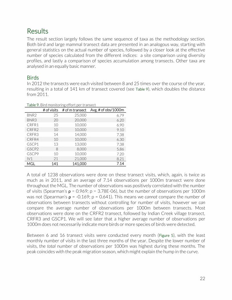
Birds In 2012 the transects were each visited between 8 and 25 times over the course of the year, resulting in a total of 141 km of transect covered (see Table 9), which doubles the distance from 2011. Table 9. Bird monitoring effort per transect

# of visits # of m transect Avg. # of obs/1000m

BNR2 25 25,000 6.79 BNR3 20 20,000 6.20 CRFR1 10 10,000 6.90 CRFR2 10 10,000 9.10 CRFR3 14 14,000 7.38 CRFR4 10 10,000 6.30 GSCP1 13 13,000 7.38 GSCP2 8 8,000 5.86 GSCP9 10 10,000 7.20 IV1 21 21,000 8.21

MGL 141 141,000 7.14

A total of 1238 observations were done on these transect visits, which, again, is twice as much as in 2011, and an average of 7.14 observations per 1000m transect were done throughout the MGL. The number of observations was positively correlated with the number of visits (Spearman’s ρ = 0.969; p = 3.78E-06), but the number of observations per 1000m was not (Spearman’s ρ = -0.169; p = 0.641). This means we cannot compare the number of observations between transects without controlling for number of visits, however we can compare the average number of observations per 1000m between transects. Most observations were done on the CRFR2 transect, followed by Indian Creek village transect, CRFR3 and GSCP1. We will see later that a higher average number of observations per 1000m does not necessarily indicate more birds or more species of birds were detected. Between 6 and 16 transect visits were conducted every month (Figure 5), with the least monthly number of visits in the last three months of the year. Despite the lower number of visits, the total number of observations per 1000m was highest during these months. The peak coincides with the peak migration season, which might explain the hump in the curve.

23

Figure 5. Bird monitoring effort in 2012

Target species richness Our list of target species for birds is biased towards forest species, but does contain disturbance indicators and savannah species. Hence, we are able to put the three habitat covered by the transects next to each other (Figure 6). 14.63 target species were detected on an average forest transect, about 15 on the Savannah transect and just over 10 on the Village lands transect. Importantly, given the openness of the Savannah and Village lands habitat as compared to the forest habitat, we would expect the visibility and sound travel distance to be greater and thus the species richness estimate for Village lands and Savannah to be inflated.

Figure 6. Average target bird species richness per transect

0.00

2.00

4.00

6.00

8.00

10.00

12.00

14.00

16.00

0

2

4

6

8

10

12

14

16

18

Jan Feb Mar Apr May Jun Jul Aug Sep Oct Nov Dec

No

. Ob

serv

ati

on

s/1

00

0m

No

. vis

its

# of visits performed # of obs/1000m

0

2

4

6

8

10

12

14

16

Forest Savannah Village lands

Av

era

ge

ta

rge

t sp

eci

es

rich

ne

ss p

er

tra

nse

ct

24

Therefore, the only valid conclusion from Figure 6 is that less of our target species were found on Village lands in 2012. All forest transects combined yielded a total of 24 target species, and there was no species detected in the savannah or village land transects that was not detected in the forest transects. However, we cannot conclude from this that, across the board, village lands contain less birds or less species of birds than the forest that surrounds them. Since the target species list is biased towards forest species, village lands might be richer in non-forest species that are not recorded during the monitoring. Species accumulation curves and rarefaction curves As in previous years, we have calculated a species accumulation curve that averages the number of species accumulated on subsequent visits across all transects (Figure 7). This tells us that, in contrast to 2011, species accumulation seems to reach a plateau around 13 species around the 10th visit. 2011 reached an average of 15 species by 15 visits.

Figure 7. Bird species accumulation curve

However, this accumulation curve has limited value in our monitoring methods, as explained in the methodology section. Therefore, instead of predicting the total species richness of each transect using accumulation curves, we use rarefaction curves to take a look from the opposite direction (see Figure 8). Starting from the right-hand side of the plot, we look for the transect that has the lowest number of samples (in this case 8 samples from GSCP2), at which point we can compare all the transects’ expected species accumulation.

0

2

4

6

8

10

12

14

0 1 2 3 4 5 6 7 8 9 10 11 12 13 14 15 16 17 18 19 20 21 22 23 24 25

# of transect visits

# of transects Average # of species

25

Figure 8. Sample-based rarefaction curves for all transects

We discover that CRFR2 and CRFR4 accumulated most species, around 16 and 14 respectively. CRFR1, CRFR3, GSCP1, GSCP2 all follow grouped together around 13 species, with BNR3 lagging behind slightly. BNR2 accumulates 11 species and IV1 around 9.5. Given its status as the least disturbed site, the low expected species accumulation for BNR2 is somewhat surprising. Table 10 shows the ranking in expected species richness of the transects at 8 transect visits. Diversity profiles As in 2011, CRFR2 appears to be most species rich and has limited levels of dominance, both of which indicate high level of biodiversity (Figure 9). Again somewhat surprisingly, BNR2 has lower diversity and has dropped a couple of places in ranking as compared to 2011 (see Table 10). The Indian Creek village transect (IV1) has lowest diversity and a pretty steep influence of dominance (low evenness).

5 10 15 20Number of transect visits

0

2

4

6

8

10

12

14

16

18

Exp

ect

ed

nu

mb

er

of

spe

cie

sBNR2CRFR1CRFR2

CRFR3CRFR4GSCP1

GSCP2GSCP9BNR3

IV1

Rank Transect

1 CRFR2

2 CRFR4

3 CRFR1

4 GSCP2

5 GSCP9

6 CRFR3

7 GSCP1

8 BNR3

9 BNR2

10 IV1

Table 10. Transect ranking according to expected bird species richness after 8 transect visits

26

Figure 9. Bird diversity profiles

Migratory birds We compare encounter rates of migratory birds between months of the year, to detect migratory patterns throughout the year. Encounter rates are calculated as the number of individuals sighted per 1000m of walked transect in the MGL. In this case, there was no significant correlation between the number of individuals per 1000m and the number of transect visits per month (Spearman’s ρ = -0.327; p = 0.276), which enables us to compare between months without controlling for the number of visits conducted in these months. Very similar to the results from 2011, the spring and autumn migration peaks are clearly visible in both encounter rates and Target Species Richness (Figure 10). More birds and species seem to hang around during the autumn trip southwards than on the spring trip northwards. A potential explanation could be that after the breeding season in the north, they might need more rest and feeding stops as they head south than on their return north. A remarkable difference with 2011 is the presence of some migrants throughout the year (American Redstart, Black and White Warbler, Hooded Warbler and Magnolia Warbler).

0.0 0.5 1.0 1.5 2.0 2.5 3.0 3.5Scaling factor (alpha)

0

2

4

6

8

10

12

14

16

18

Eff

ect

ive

Nu

mb

er

of

bir

d S

pec

ies

BNR2BNR3CRFR1

CRFR2CRFR3CRFR4

GSCP1GSCP2GSCP9

IV1

27

Figure 10. Migrant encounter rate and species richness throughout the year

Indicator groups Looking at Indicator groups can be done on the species level (“how many of the species in each Indicator group were detected in each habitat?”) and individual level (“how many individuals of each Indicator group – regardless of species – were detected in each habitat?”). The first option has the disadvantage that the number of species will depend on the number of visits to a certain transect. The second option omits species richness as an explanatory factor. We will have a look at both. In the village lands, considerably less Forest, Game, Pine and Wetland indicator species were detected, which might have to do with the reduced number of transect visits there, but all Migratory route indicators were present. In the savannah, less Forest and Wetland indicator species were detected and marginally less Game and, remarkably, Pine savannah species. However, even though the savannah habitat has less Pine savannah indicator species, Figure

11 shows us that it has proportionally much more individuals of these species than any other habitat or transect.

0

2

4

6

8

10

12

14

0

2

4

6

8

10

12

14

Jan Feb Mar Apr May Jun Jul Aug Sep Oct Nov Dec

Ta

rge

t sp

eci

es

rich

ne

ss

En

cou

nte

r ra

te (

# o

f in

d/

10

00

m)

Worm-eating Warbler

Wood Thrush

Swainson’s Warbler

Prothonotary Warbler

Northern Waterthrush

Magnolia warbler

Louisiana Waterthrush

Kentucky Warbler

Hooded warbler

Common Yellowthroat

Blue-gray Gnatcatcher

Black and White Warbler

American Redstart

Target species richness

28

Figure 11. Distribution of individuals among Indicator Groups

More than half of all individuals recorded on the Village lands were disturbance indicators (in this case big flocks of Plain Chachalaca), where they were only a quarter or less in the forest or the savannah. Close to half of all individuals recorded were indicators of Migratory route health, but only 1.2% of all birds in village lands were Healthy forest indicators. The village lands totally lacked any of the Game birds. Close to a third of all individuals detected on the savannah were Pine savannah indicators, but the savannah still reached 11% in Healthy forest indicators, presumably due to the proximity of the savannah transect to the forest. Quite unexpectedly over a quarter of all species recorded in forest were Healthy forest indicators. Migratory route health indicators formed more than one third of all individuals detected in the forest, but only 21% of all birds recorded in the savannah. Wetland indicators were absent from the savannah and accounted for minimal percentages of individuals in forests and village lands. In the above graph, the number of individuals is shown in brackets for each habitat. Since the number of individuals was positively correlated with the number of transect visits (Spearman’s ρ = 0.956; p = 1.46E-05), the interpretation needs to take into account the number of transect visits that were conducted within each habitat. There were 100 transect visits done in the forest habitat, only 20 in the savannah and 21 in village lands habitat. Not surprisingly, more individuals and species were observed in the forest than on the single transects in the savannah and village lands. We standardized using percentages rather than standardizing per distance (i.e. encounter rate – number of individuals per 1000m), to avoid the difference in observed number of species affecting the summed encounter rates per Indicator group. In the previous Biodiversity Synthesis Report, a roughly defined disturbance gradient among the eight forest transect was identified, which warrants a closer look at the distribution of indicator species across this gradient. Figure 12 shows the proportions of individuals

0%

10%

20%

30%

40%

50%

60%

70%

80%

90%

100%

Forest (n=992) Savannah (n=210) Village lands (n=257)

Not assigned

Wetland

Pine savannah

Migratory route health

Game

Forest health

Disturbance

29

belonging to each indicator group for all forest transects (excluding the abandoned BNR1 transect, and including the new GSCP9 transect), and puts these next to the village lands and savannah transects for reference. Note that many more factors than just this (roughly defined) disturbance level could be causing the observed pattern of the Indicator groups (e.g. weather, monitoring effort, population fluctuations), and we therefore cannot look at the details of every single transect. Instead, we will look at overarching tendencies. A rough trend is visible: the more disturbed forest transects have proportionally less Forest health and Game indicators and a higher proportion of Disturbance and Migratory route health indicators, which is taken to the extreme in the village lands transect (IV1). The savannah transect (BNR3) expectedly has a very different composition than all other transects.

Figure 12. Distribution of individuals among Indicator Groups, looked at per transect. From the left, the first 8 transects indicate a habitat disturbance gradient in the forest. The next transect is on village lands, the last one in savannah.

Again the number of individuals detected on the different transects is shown in brackets. BNR2, BNR3 and IV1 all had over 20 transect visits, whereas all other transects were visited 14 times or less (see Table 9). Trends in the forests of the Maya Golden Landscape Lining up the Target species richness over the years, an increase is visible over the last two, arguably three, years (Figure 13). This is also reflected in the diversity profiles (Figure 14), where the last three years have highest diversity. Evenness of relative abundances (or dominance of a small number of species) seems to be comparable throughout the years.

Habitat disturbance

0%

10%

20%

30%

40%

50%

60%

70%

80%

90%

100%

Not assigned

Wetland

Pine savannah

Migratory route health

Game

Forest health

Disturbance

30

Figure 13. Target bird species richness since 2007 (Number of transect visits in brackets)

The trend of increasing species richness doesn’t necessarily reflect an increase in habitat quality or suitability. It might also be due to the combined effect of the increased identification skills for migratory birds among the rangers following bird training by visiting experts and using audio-visual materials, the increased supervision during transect visits and the improvement of data entry and handling systems and skills at Ya’axché.

Figure 14. Diversity profiles for the bird community of the Maya Golden Landscape since 2007 (Number of transect visits in brackets)

0

5

10

15

20

25

30

2007 (36) 2008 (54) 2009 (32) 2010 (49) 2011 (73) 2012 (100)

Ta

rge

t sp

eci

es

rich

ne

ss

0.0 0.5 1.0 1.5 2.0 2.5 3.0 3.5Scaling factor (alpha)

0

3

6

9

12

15

18

21

24

27

Eff

eci

tve

Nu

mb

er

of

bir

d S

pec

ies

2007_(36)2008_(54)2009_(32)

2010_(49)2011_(73)2012_(100)

31

To single out the most diverse transects in the Maya Golden Landscape with respect to birds, we combine the ranking of transects from the last three years, based on the rarefaction results from the respective years (Table 11). In 2010 and 2011 transect ranking was evaluated after 6 visits, in 2012 after 8 visits. We chose to ignore the first three years due to the limited number of visits per transect, which makes rarefaction not applicable. We notice that CRFR2 leads the species richness ranking in all three years, while both CRFR3 and CRFR1 feature two times in the top three of the ranking. CRFR4 follows two times on the fourth place and once in the top three. The comparison of distribution of individual birds among Indicator Groups is probably the most informative comparison we can make to detect changes in habitat quality (Figure 15). In this case, a shift from a

higher Disturbance indicator percentage in the first three years towards a higher Migration route health indicator percentage in the last three years can be seen over the years. However, this is again most likely due to the increased capacities in the field ranger team in identifying migratory birds, rather than an increase of habitat quality, as described above for the species richness.

Figure 15. Distribution of individuals among Indicator Groups over the years 2007-2012

0%

10%

20%

30%

40%

50%

60%

70%

80%

90%

100%

2007 (n=363)

2008 (n=925)

2009 (n=461)

2010 (n=514)

2011 (n=749)

2012 (n=992)

Not assigned

Wetland

Pine savannah

Migratory route health

Game

Forest health

Disturbance

Rank 2010 (6) 2011 (6) 2012 (8)

1 CRFR2 CRFR2 CRFR2

2 CRFR1 BNR2 CRFR4

3 CRFR3 CRFR3 CRFR1

4 CRFR4 CRFR4 GSCP2

5 GSCP2 GSCP1 GSCP9

6 BNR1 CRFR1 CRFR3

7 GSCP1 GSCP2 GSCP1

8 BNR3

9 BNR2

10 IV1

Table 11. Transect ranking according To expected number of species from the rarefaction results. (No. of transect visits at evaluation in brackets)

32

Large mammals In general the number of transect visits performed per transect is half of that for bird monitoring: from four to thirteen times, resulting in a total of 71km transect covered (Table

12). A total of 528 observations of mammals signs were done, with on average 5.03 observations per 1000m transect in the Maya Golden Landscape. Table 12. Mammal monitoring effort per transect

# of visits # of m transect Avg. # of obs/1000m

BNR2 13 13000 5.62 BNR3 10 10000 4.00 CRFR1 5 5000 3.80 CRFR2 5 5000 5.80 CRFR3 7 7000 4.43 CRFR4 5 5000 6.80 GSCP1 6 6000 7.60 GSCP2 4 4000 7.75 GSCP9 5 5000 3.60 IV1 11 11000 2.64

MGL 71 71000 5.03

On a monthly basis, between three and eight transect visits were conducted (Figure 16). As in birds, the average number of mammal observations per 1000m was not correlated to the number of transect visits (Spearman’s ρ = -0206; p = 0.499). The observation peak detected in the summer of 2011 (presumably due to the fact that tracks of mammals are usually more readily detected during the wet season) was not detected in 2012.

Figure 16. Mammal monitoring effort in 2012

Target species richness In contrast to the birds, visibility and sound cues are less important for most target mammal species, because they are usually detected indirectly using tracks and other signs. Therefore,

0

2

4

6

8

10

12

Jan Feb Mar Apr May Jun Jul Aug Sept Oct Nov Dec

# of visits performed # of obs/1000m

33

we do not expect the openness of the Savannah and Village lands habitat to inflate the number of species observed. We notice a slight decrease in average number of target species observed per transect from Forest to Village lands habitat (Figure 17), indicating that of any given transect, we would expect the ones located in forest to have the highest large mammal species diversity.

Figure 17. Average target mammal species richness per transect

All of the total 17 mammal species were observed in the Forest, while only seven and six were recorded in the Savannah and on Village lands, respectively. The difference in total number of species between Forest and the other two habitat types is in presumably due to the difference in number of transect visit and area covered (8 forest transects, 1 savannah and 1 village lands transect). Species accumulation and rarefaction curves In 2011, the species accumulation curve (average species accumulation per visit across all transects) had reached 10 by the eighth visit. This year, we are nearing the same number after 11 visits (Figure 18). The overall shape of the curve is very similar though, perhaps indicating that there are about eight species that are detected reasonably often, after which the rarer species are detected at a much slower pace (after around 7-8 visits). The rarefaction curves tell us that the higher species richness in Forest transects is generally present from the first visit (Figure 19). The Savannah transect (BNR3) and the Village lands transect (IV1) lag behind in species accumulation.

0

1

2

3

4

5

6

7

8

9

10

Forest Savannah Village lands

Av

era

ge

Ta

rge

t sp

eci

es

rich

ne

ss p

er

tra

nse

ct

34

Figure 18. Mammal species accumulation curve

Figure 19. Sample-based rarefaction curves for large mammals

After the fourth visit, BNR2 leads the ranking in expected target species richness, followed by CRFR4 (Table 13). In contrast to birds, mammals seem to be more diverse on the GSCP transects than on some of the CRFR transects.

0

2

4

6

8

10

12

0 1 2 3 4 5 6 7 8 9 10 11 12 13

# of transect visits

# of transects Average # of species

2 4 6 8 10 12Number of transect visits

0

2

4

6

8

10

12

14

16

18

Exp

ect

ed

sp

eci

es

rich

ne

ss

BNR2BNR3CRFR1

CRFR2CRFR3CRFR4

GSCP1GSCP2GSCP9

IV1

35

Diversity profile The impact of large herds of White-lipped peccary causes the diversity profiles of BNR2 and CRFR3 to drop significantly: their numbers create unevenly distributed relative abundances (Figure 20). As scaling factor α increases, the dominance of the White-lipped peccaries weighs in heavier and reduces the Effective Number mammal Species. The similar effect observed in the Village lands transect (IV1) is due to a disproportional amount of Agouti and Nine-banded armadillo, as we will see in the indicator group results on the next pages.

Figure 20. Mammal diversity profiles

Indicator groups On an average forest transect, more Forest indicator species were detected than in other habitat (Table 14). The savannah transect had slightly less Game species detected, and the village lands had

no signs of Tapir presence, the only Wetland indicator species detected. Overall, the average forest transect had highest target species richness (see also Figure 17). Looking at the percentage of individuals belonging to each indicator group (Figure 21), we notice the similarity between the forest and the savannah, with a nearly equal share of Forest health and Game indicators, likely due again to the proximity of the savannah transect (BNR3) to the forest. We also notice the drop in Forest indicators on Village lands, and the large proportion of Game species among the mammals detected on Village lands.

0.0 0.5 1.0 1.5 2.0 2.5 3.0 3.5Scaling factor (alpha)

0

2

4

6

8

10

12

14

16

18

Eff

ect

ive

Nu

mb

er

of

mam

ma

l Sp

eci

es

BNR2BNR3CRFR1

CRFR2CRFR3CRFR4

GSCP1GSCP2GSCP9

IV1

Rank Transect

1 BNR2

2 CRFR4

3 GSCP1

4 GSCP2

5 CRFR3

6 CRFR1

7 CRFR2

8 GSCP9

9 BNR3

10 IV1

Table 13. Transect ranking according to expected bird species richness after 8 transect visits

36

Figure 21. Distribution of individuals among Indicator Groups

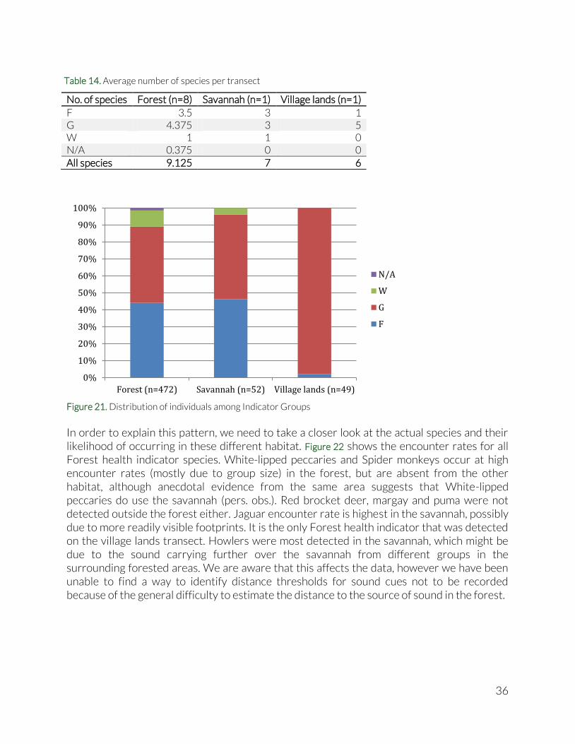
In order to explain this pattern, we need to take a closer look at the actual species and their likelihood of occurring in these different habitat. Figure 22 shows the encounter rates for all Forest health indicator species. White-lipped peccaries and Spider monkeys occur at high encounter rates (mostly due to group size) in the forest, but are absent from the other habitat, although anecdotal evidence from the same area suggests that White-lipped peccaries do use the savannah (pers. obs.). Red brocket deer, margay and puma were not detected outside the forest either. Jaguar encounter rate is highest in the savannah, possibly due to more readily visible footprints. It is the only Forest health indicator that was detected on the village lands transect. Howlers were most detected in the savannah, which might be due to the sound carrying further over the savannah from different groups in the surrounding forested areas. We are aware that this affects the data, however we have been unable to find a way to identify distance thresholds for sound cues not to be recorded because of the general difficulty to estimate the distance to the source of sound in the forest.

0%

10%

20%

30%

40%

50%

60%

70%

80%

90%

100%

Forest (n=472) Savannah (n=52) Village lands (n=49)

N/A

W

G

F

No. of species Forest (n=8) Savannah (n=1) Village lands (n=1)

F 3.5 3 1 G 4.375 3 5 W 1 1 0 N/A 0.375 0 0 All species 9.125 7 6

Table 14. Average number of species per transect

37

Figure 22. Encounter rate of all Forest health indicator species

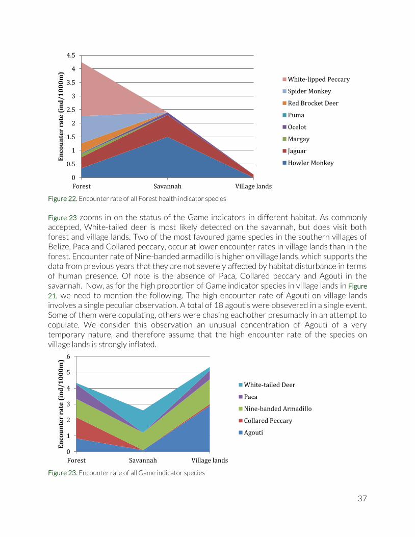
Figure 23 zooms in on the status of the Game indicators in different habitat. As commonly accepted, White-tailed deer is most likely detected on the savannah, but does visit both forest and village lands. Two of the most favoured game species in the southern villages of Belize, Paca and Collared peccary, occur at lower encounter rates in village lands than in the forest. Encounter rate of Nine-banded armadillo is higher on village lands, which supports the data from previous years that they are not severely affected by habitat disturbance in terms of human presence. Of note is the absence of Paca, Collared peccary and Agouti in the savannah. Now, as for the high proportion of Game indicator species in village lands in Figure

21, we need to mention the following. The high encounter rate of Agouti on village lands involves a single peculiar observation. A total of 18 agoutis were obsevered in a single event. Some of them were copulating, others were chasing eachother presumably in an attempt to copulate. We consider this observation an unusual concentration of Agouti of a very temporary nature, and therefore assume that the high encounter rate of the species on village lands is strongly inflated.

Figure 23. Encounter rate of all Game indicator species

0

0.5

1

1.5

2

2.5

3

3.5

4

4.5

Forest Savannah Village lands

En

cou

nte

r ra

te (

ind

/1

00

0m

)

White-lipped Peccary

Spider Monkey

Red Brocket Deer

Puma

Ocelot

Margay

Jaguar

Howler Monkey

0

1

2

3

4

5

6

Forest Savannah Village lands

En

cou

nte

r ra

te (

ind

/1

00

0m

)

White-tailed Deer

Paca

Nine-banded Armadillo

Collared Peccary

Agouti

38

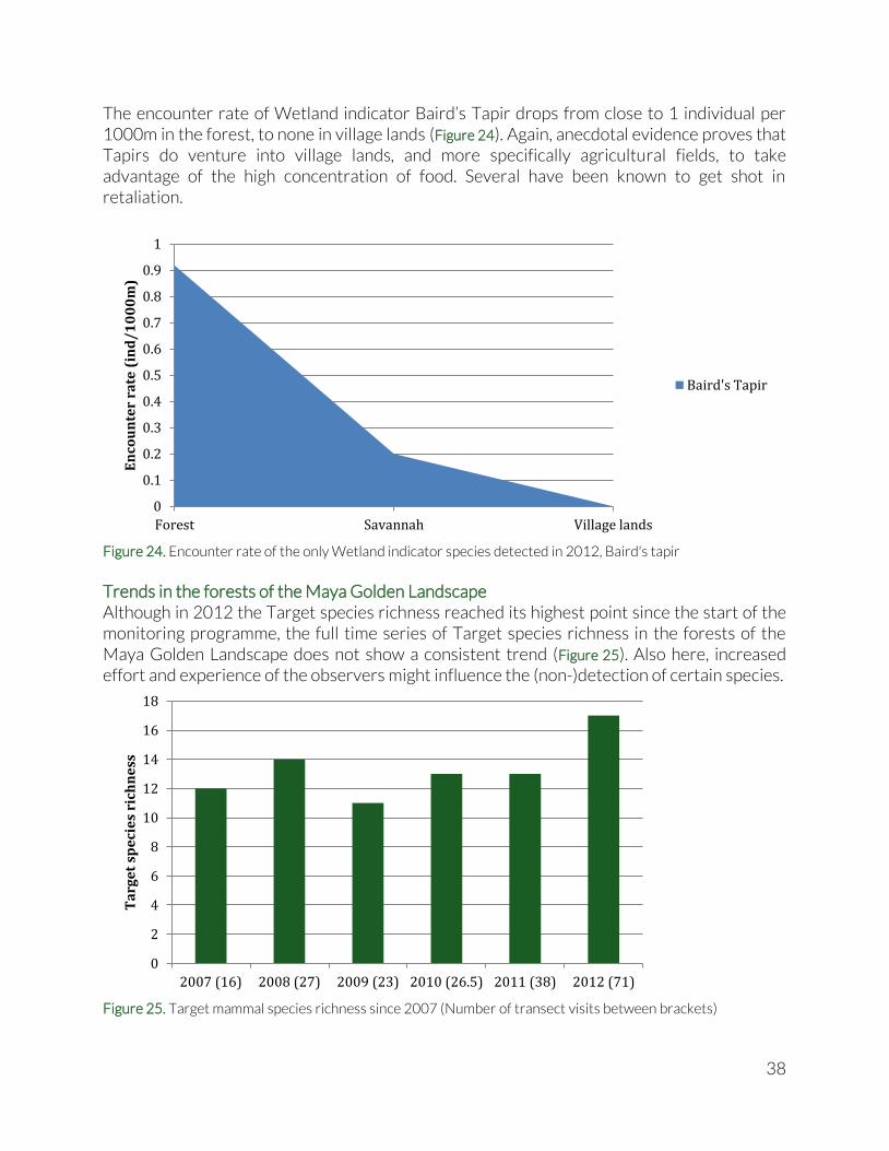
The encounter rate of Wetland indicator Baird’s Tapir drops from close to 1 individual per 1000m in the forest, to none in village lands (Figure 24). Again, anecdotal evidence proves that Tapirs do venture into village lands, and more specifically agricultural fields, to take advantage of the high concentration of food. Several have been known to get shot in retaliation.

Figure 24. Encounter rate of the only Wetland indicator species detected in 2012, Baird's tapir

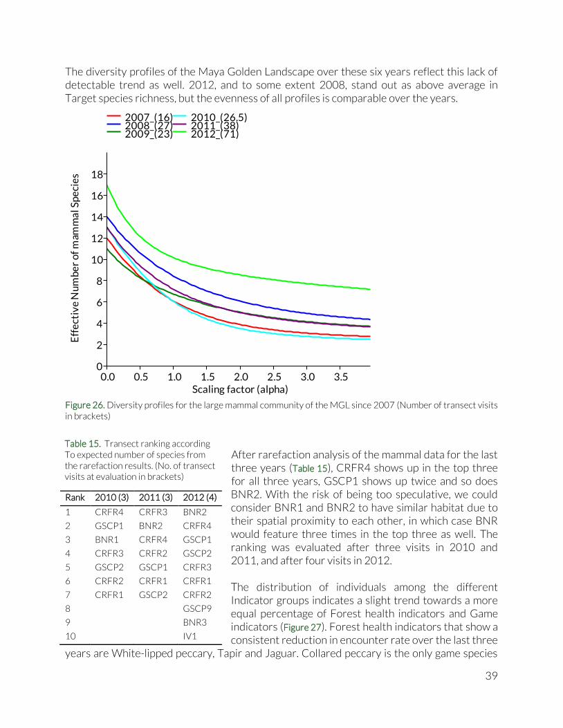
Trends in the forests of the Maya Golden Landscape Although in 2012 the Target species richness reached its highest point since the start of the monitoring programme, the full time series of Target species richness in the forests of the Maya Golden Landscape does not show a consistent trend (Figure 25). Also here, increased effort and experience of the observers might influence the (non-)detection of certain species.

Figure 25. Target mammal species richness since 2007 (Number of transect visits between brackets)

0

0.1

0.2

0.3

0.4

0.5

0.6

0.7

0.8

0.9

1

Forest Savannah Village lands

En

cou

nte

r ra

te (

ind

/1

00

0m

)

Baird's Tapir

0

2

4

6

8

10

12

14

16

18

2007 (16) 2008 (27) 2009 (23) 2010 (26.5) 2011 (38) 2012 (71)

Ta

rge

t sp

eci

es

rich

ne

ss

39

The diversity profiles of the Maya Golden Landscape over these six years reflect this lack of detectable trend as well. 2012, and to some extent 2008, stand out as above average in Target species richness, but the evenness of all profiles is comparable over the years.

Figure 26. Diversity profiles for the large mammal community of the MGL since 2007 (Number of transect visits in brackets)

After rarefaction analysis of the mammal data for the last three years (Table 15), CRFR4 shows up in the top three for all three years, GSCP1 shows up twice and so does BNR2. With the risk of being too speculative, we could consider BNR1 and BNR2 to have similar habitat due to their spatial proximity to each other, in which case BNR would feature three times in the top three as well. The ranking was evaluated after three visits in 2010 and 2011, and after four visits in 2012. The distribution of individuals among the different Indicator groups indicates a slight trend towards a more equal percentage of Forest health indicators and Game indicators (Figure 27). Forest health indicators that show a consistent reduction in encounter rate over the last three

years are White-lipped peccary, Tapir and Jaguar. Collared peccary is the only game species

0.0 0.5 1.0 1.5 2.0 2.5 3.0 3.5Scaling factor (alpha)

0

2

4

6

8

10

12

14

16

18

Eff

ect

ive

Nu

mb

er

of

mam

ma

l Sp

eci

es

2007_(16)2008_(27)2009_(23)

2010_(26.5)2011_(38)2012_(71)

Rank 2010 (3) 2011 (3) 2012 (4)

1 CRFR4 CRFR3 BNR2

2 GSCP1 BNR2 CRFR4

3 BNR1 CRFR4 GSCP1

4 CRFR3 CRFR2 GSCP2

5 GSCP2 GSCP1 CRFR3

6 CRFR2 CRFR1 CRFR1

7 CRFR1 GSCP2 CRFR2

8 GSCP9

9 BNR3

10 IV1

Table 15. Transect ranking according To expected number of species from the rarefaction results. (No. of transect visits at evaluation in brackets)

40

that shows a consistent increase over the same time period, suggesting that the shift in percentage is mostly due to a drop in numbers of Forest indicators. But again, we cannot exclude the influence of improved effort, skills and systems on the time series. We might just be getting a more realistic image.

Figure 27. Distribution of individuals among Indicator Groups

Camera trapping A minimum of 626 of ‘trapping nights’ (the sum of all nights any one camera was active) have been logged. However a number of deployments have been inadequately documented, which makes an accurate count of trapping nights impossible, hence the reason for the minimum number of trapping nights. From the recorded 626, 151 nights were at four sites in Bladen Nature Reserve, and the remaining 475 at 7 sites in Golden Stream Corridor Preserve. We counted three bird species and at least 15 mammal species in the MGL (Table 16). The table counts the number of passes in front of the camera, rather than the number of pictures, because some animals get photographed several times while passing the camera only once. We used the arbitrary cut-off point of 30min between photographs to assume a different passing event. Group size indicates the

0%

10%

20%

30%

40%

50%

60%

70%

80%

90%

100%

2007 (n=120)

2008 (n=214)

2009 (n=167)

2010 (n=317)

2011 (n=366)

2012 (n=472)

N/A

W

G

F

# of passes BNR GSCP Group size

Bir

ds

Bare-throated tiger heron --- 2 1 Currasow 2 6 1.13 Limpkin --- 1 1

Mam

mal

s

Agouti 3 9 1 Coatimundi 2 5 1 Collared peccary 2 2 2 Gibnut --- 2 1 Jaguar 1 29 1 Jaguarundi --- 2 1 Ocelot 1 7 1 Possum 2 3 1 Puma 3 11 1 Red brocket deer 1 9 1 Striped hog-nosed skunk --- 1 1 Tapir 3 6 1 White-lipped peccary 8 --- 5.13 White-tailed deer --- 1 1

Unidentified 3 3 1

Total 31 99 1.3

Species richness 12 17 -

Table 16. Species diversity results from the 2012 camera trapping survey. (see text for explanation of ‘Group size’)

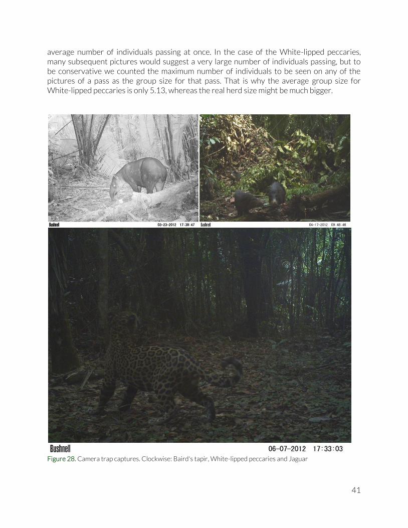
41

average number of individuals passing at once. In the case of the White-lipped peccaries, many subsequent pictures would suggest a very large number of individuals passing, but to be conservative we counted the maximum number of individuals to be seen on any of the pictures of a pass as the group size for that pass. That is why the average group size for White-lipped peccaries is only 5.13, whereas the real herd size might be much bigger.

Figure 28. Camera trap captures. Clockwise: Baird's tapir, White-lipped peccaries and Jaguar

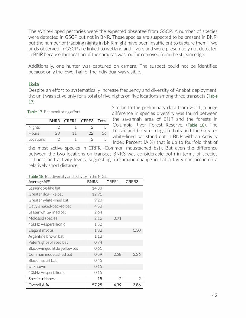
42

The White-lipped peccaries were the expected absentee from GSCP. A number of species were detected in GSCP but not in BNR. These species are suspected to be present in BNR, but the number of trapping nights in BNR might have been insufficient to capture them. Two birds observed in GSCP are linked to wetland and rivers and were presumably not detected in BNR because the location of the cameras was too far removed from the stream edge. Additionally, one hunter was captured on camera. The suspect could not be identified because only the lower half of the individual was visible.

Bats Despite an effort to systematically increase frequency and diversity of Anabat deployment, the unit was active only for a total of five nights on five locations among three transects (Table

17). Similar to the preliminary data from 2011, a huge difference in species diversity was found between the savannah area of BNR and the forests in Columbia River Forest Reserve. (Table 18). The Lesser and Greater dog-like bats and the Greater white-lined bat stand out in BNR with an Activity Index Percent (AI%) that is up to fourfold that of

the most active species in CRFR (Common moustached bat). But even the difference between the two locations on transect BNR3 was considerable both in terms of species richness and activity levels, suggesting a dramatic change in bat activity can occur on a relatively short distance. Table 18. Bat diversity and activity in the MGL

Average AI% BNR3 CRFR1 CRFR3

Lesser dog-like bat 14.38

Greater dog-like bat 12.91

Greater white-lined bat 9.20

Davy's naked-backed bat 4.53

Lesser white-lined bat 2.64

Molossid species 2.16 0.91

45kHz Vespertillionid 1.52

Elegant myotis 1.33 0.30

Argentine brown bat 1.13

Peter's ghost-faced bat 0.74

Black-winged little yellow bat 0.61

Common moustached bat 0.59 2.58 3.26

Black mastiff bat 0.45

Unknown 0.15

40kHz Vespertillionid 0.15

Species richness 15 2 2

Overall AI% 57.25 4.39 3.86

BNR3 CRFR1 CFRF3 Total

Nights 2 1 2 5

Hours 23 11 22 56

Locations 2 1 2 5

Table 17. Bat monitoring effort

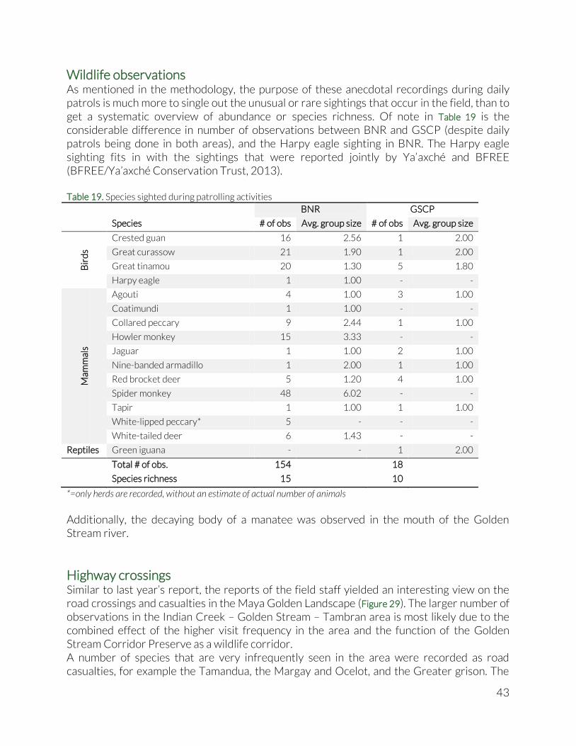
43

Wildlife observations As mentioned in the methodology, the purpose of these anecdotal recordings during daily patrols is much more to single out the unusual or rare sightings that occur in the field, than to get a systematic overview of abundance or species richness. Of note in Table 19 is the considerable difference in number of observations between BNR and GSCP (despite daily patrols being done in both areas), and the Harpy eagle sighting in BNR. The Harpy eagle sighting fits in with the sightings that were reported jointly by Ya’axché and BFREE (BFREE/Ya’axché Conservation Trust, 2013). Table 19. Species sighted during patrolling activities

BNR GSCP

Species # of obs Avg. group size # of obs Avg. group size

Bir

ds

Crested guan 16 2.56 1 2.00

Great curassow 21 1.90 1 2.00

Great tinamou 20 1.30 5 1.80

Harpy eagle 1 1.00 - -

Mam

mal

s

Agouti 4 1.00 3 1.00

Coatimundi 1 1.00 - -

Collared peccary 9 2.44 1 1.00

Howler monkey 15 3.33 - -

Jaguar 1 1.00 2 1.00

Nine-banded armadillo 1 2.00 1 1.00

Red brocket deer 5 1.20 4 1.00

Spider monkey 48 6.02 - -

Tapir 1 1.00 1 1.00

White-lipped peccary* 5 - - -

White-tailed deer 6 1.43 - -

Reptiles Green iguana - - 1 2.00

Total # of obs. 154 18

Species richness 15 10

*=only herds are recorded, without an estimate of actual number of animals

Additionally, the decaying body of a manatee was observed in the mouth of the Golden Stream river.

Highway crossings Similar to last year’s report, the reports of the field staff yielded an interesting view on the road crossings and casualties in the Maya Golden Landscape (Figure 29). The larger number of observations in the Indian Creek – Golden Stream – Tambran area is most likely due to the combined effect of the higher visit frequency in the area and the function of the Golden Stream Corridor Preserve as a wildlife corridor. A number of species that are very infrequently seen in the area were recorded as road casualties, for example the Tamandua, the Margay and Ocelot, and the Greater grison. The

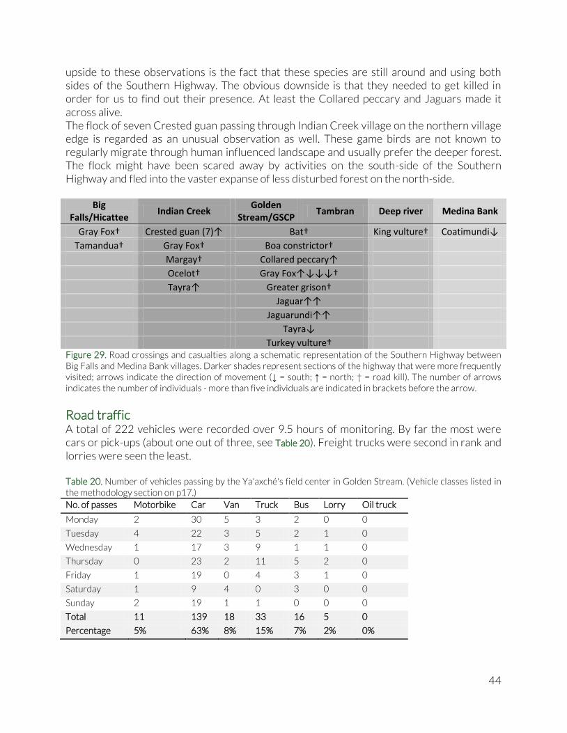
44

upside to these observations is the fact that these species are still around and using both sides of the Southern Highway. The obvious downside is that they needed to get killed in order for us to find out their presence. At least the Collared peccary and Jaguars made it across alive. The flock of seven Crested guan passing through Indian Creek village on the northern village edge is regarded as an unusual observation as well. These game birds are not known to regularly migrate through human influenced landscape and usually prefer the deeper forest. The flock might have been scared away by activities on the south-side of the Southern Highway and fled into the vaster expanse of less disturbed forest on the north-side.

Big Falls/Hicattee

Indian Creek Golden

Stream/GSCP Tambran Deep river Medina Bank

Gray Fox† Crested guan (7)↑ Bat† King vulture† Coatimundi↓

Tamandua† Gray Fox† Boa constrictor†

Margay† Collared peccary↑

Ocelot† Gray Fox↑↓↓↓†

Tayra↑ Greater grison†

Jaguar↑↑

Jaguarundi↑↑

Tayra↓

Turkey vulture† Figure 29. Road crossings and casualties along a schematic representation of the Southern Highway between Big Falls and Medina Bank villages. Darker shades represent sections of the highway that were more frequently visited; arrows indicate the direction of movement (↓ = south; ↑ = north; † = road kill). The number of arrows indicates the number of individuals - more than five individuals are indicated in brackets before the arrow.

Road traffic A total of 222 vehicles were recorded over 9.5 hours of monitoring. By far the most were cars or pick-ups (about one out of three, see Table 20). Freight trucks were second in rank and lorries were seen the least. Table 20. Number of vehicles passing by the Ya'axché's field center in Golden Stream. (Vehicle classes listed in the methodology section on p17.)

No. of passes Motorbike Car Van Truck Bus Lorry Oil truck

Monday 2 30 5 3 2 0 0

Tuesday 4 22 3 5 2 1 0

Wednesday 1 17 3 9 1 1 0

Thursday 0 23 2 11 5 2 0

Friday 1 19 0 4 3 1 0

Saturday 1 9 4 0 3 0 0

Sunday 2 19 1 1 0 0 0

Total 11 139 18 33 16 5 0

Percentage 5% 63% 8% 15% 7% 2% 0%

45

Temporal spread of activities was considered at two different scales: daily and weekly (Figure

30A&B) Throughout the day, most vehicles passed during the afternoon hours, with a marked spike in trucks passing by. No lorries were recorded in morning hours. Throughout the week, traffic density (vehicles/hour) seemed to spike on Mondays and Thursdays, with lows on Fridays and Saturdays. The middle days of the week seemed to have the heaviest truck traffic, whereas Mondays and Sundays had the most car/pickup traffic. In general, we see a traffic density of 23.05 vehicles per hour on an average day, ranging between 17 and 28.67.

Land snails As a preliminary try-out to familiarise two rangers with the methodology, a test plot was set up close to the BNR ranger base. Soon after that, a set of two plots (slope and valley) was set up close to the eastern boundary of Bladen Nature Reserve in the proximity of the Belize Foundation for Research and Environmental Education (see Figure 31). These two eastern-most plots were located inside the two permanent sample plots (PSP) for vegetation monitoring (see next section). Two additional sets were established in the Richardson’s Creek and Quebrada de Oro areas along the Bladen river. Samples were successfully collected and stored, and data handling by the rangers was adequate. All information on canopy cover, ground cover, microhabitat and weather was useful and correct. However the initial species identification training proved to be insufficient to achieve a high enough standard for successful processing of the samples by our ranger team. Over one third of all identifications done by the rangers were cross-checked by snail specialist Dan Dourson to obtain an idea of the validity of the species data. The comparison of both datasets indicated that our ranger team overestimated the amount of species by ca. 20% and the number of identifiable individuals by ca. two-thirds.

0

5

10

15

20

25

30

Morning Afternoon Evening

No

. of

pa

sse

s p

er

ho

ur

Lorry

Bus

Truck

Van

Car/Pick-up

Motorbike

Figure 30. Average number of vehicles passing per hour, grouped per part of day (A), and day of the week (B)

A B

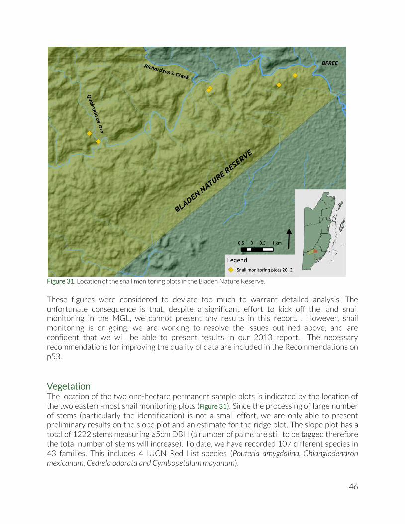
46

Figure 31. Location of the snail monitoring plots in the Bladen Nature Reserve.

These figures were considered to deviate too much to warrant detailed analysis. The unfortunate consequence is that, despite a significant effort to kick off the land snail monitoring in the MGL, we cannot present any results in this report. . However, snail monitoring is on-going, we are working to resolve the issues outlined above, and are confident that we will be able to present results in our 2013 report. The necessary recommendations for improving the quality of data are included in the Recommendations on p53.

Vegetation The location of the two one-hectare permanent sample plots is indicated by the location of the two eastern-most snail monitoring plots (Figure 31). Since the processing of large number of stems (particularly the identification) is not a small effort, we are only able to present preliminary results on the slope plot and an estimate for the ridge plot. The slope plot has a total of 1222 stems measuring ≥5cm DBH (a number of palms are still to be tagged therefore the total number of stems will increase). To date, we have recorded 107 different species in 43 families. This includes 4 IUCN Red List species (Pouteria amygdalina, Chiangiodendron mexicanum, Cedrela odorata and Cymbopetalum mayanum).

47

Weather For both locations with manual stations, several days of the year lacked data on rainfall, relative humidity and temperature (see below). Additionally, the rain gauges state two different volume units (mm and inches), which has inadvertently lead to both being used interchangeably in the records. This has definitely introduced error in the data which is impossible to trace, and thus can have an effect of unknown size on the results. Methods to impute the missing data from neighbouring weather stations or historic data from the same weather station exist (e.g. Acock & Pachepsky, 1999; Lo Presti et al., 2010), however these were not used for the current dataset due to time constraints. Bladen Nature Reserve ranger base Weather data from the BNR ranger base was moderately complete. 284 days of the year (77.6%) were recorded, and yielded an annual rainfall of 3209.07mm. Given the missing data for nearly one quarter of the year, the total amount of rainfall for 2012 is considerable.

Figure 32. Detail of the mean rainfall map presented earlier (Figure 4 on p21)

When compared to long-term reference values (Figure 32), our observed rainfall figures are well above the average annual rainfall in the area. Adding estimates for the large amount of missing data would increase the total rainfall at BNR ranger base to even higher levels. Additionally, even though the data coverage is much lower in BNR than in GSCP (see below), the total rainfall for 2012 is considerably higher. This is unexpected given GSCP’s more southward location. This could be an indication of a local maximum thus far gone undetected by the existing weather station network, or it could be due to extremely wet periods in BNR this year, but it could also be a result introduced by the simultaneous use of different measurement units, or a combination of these. Nonetheless, the rainfall pattern throughout the year roughly follows the expected pattern (Figure 33), indicating there is some validity to the data collected.

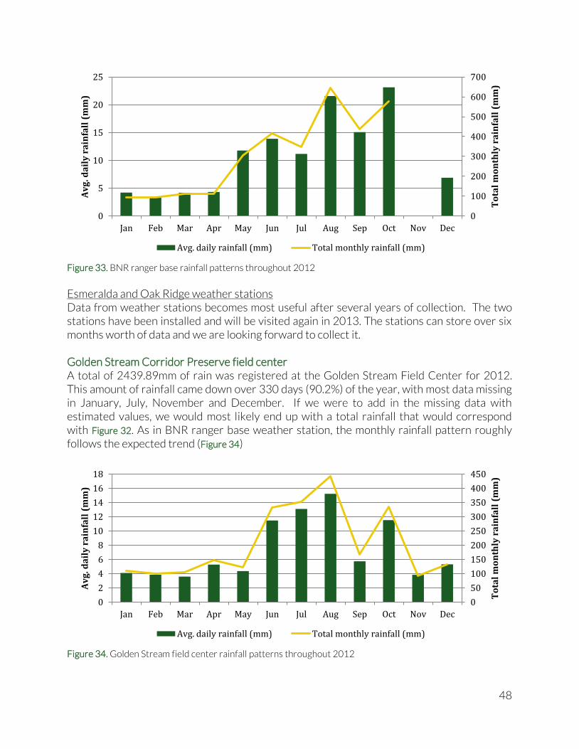
48

Figure 33. BNR ranger base rainfall patterns throughout 2012

Esmeralda and Oak Ridge weather stations Data from weather stations becomes most useful after several years of collection. The two stations have been installed and will be visited again in 2013. The stations can store over six months worth of data and we are looking forward to collect it. Golden Stream Corridor Preserve field center A total of 2439.89mm of rain was registered at the Golden Stream Field Center for 2012. This amount of rainfall came down over 330 days (90.2%) of the year, with most data missing in January, July, November and December. If we were to add in the missing data with estimated values, we would most likely end up with a total rainfall that would correspond with Figure 32. As in BNR ranger base weather station, the monthly rainfall pattern roughly follows the expected trend (Figure 34)

Figure 34. Golden Stream field center rainfall patterns throughout 2012

0

100

200

300

400

500

600

700

0

5

10

15

20

25

Jan Feb Mar Apr May Jun Jul Aug Sep Oct Nov Dec

To

tal

mo

nth

ly r

ain

fall

(m

m)

Av

g. d

ail

y r

ain

fall

(m

m)

Avg. daily rainfall (mm) Total monthly rainfall (mm)

0

50

100

150

200

250

300

350

400

450

0

2

4

6

8

10

12

14

16

18

Jan Feb Mar Apr May Jun Jul Aug Sep Oct Nov Dec

To

tal

mo

nth

ly r

ain

fall

(m

m)

Av

g. d

ail

y r

ain

fall

(m

m)

Avg. daily rainfall (mm) Total monthly rainfall (mm)

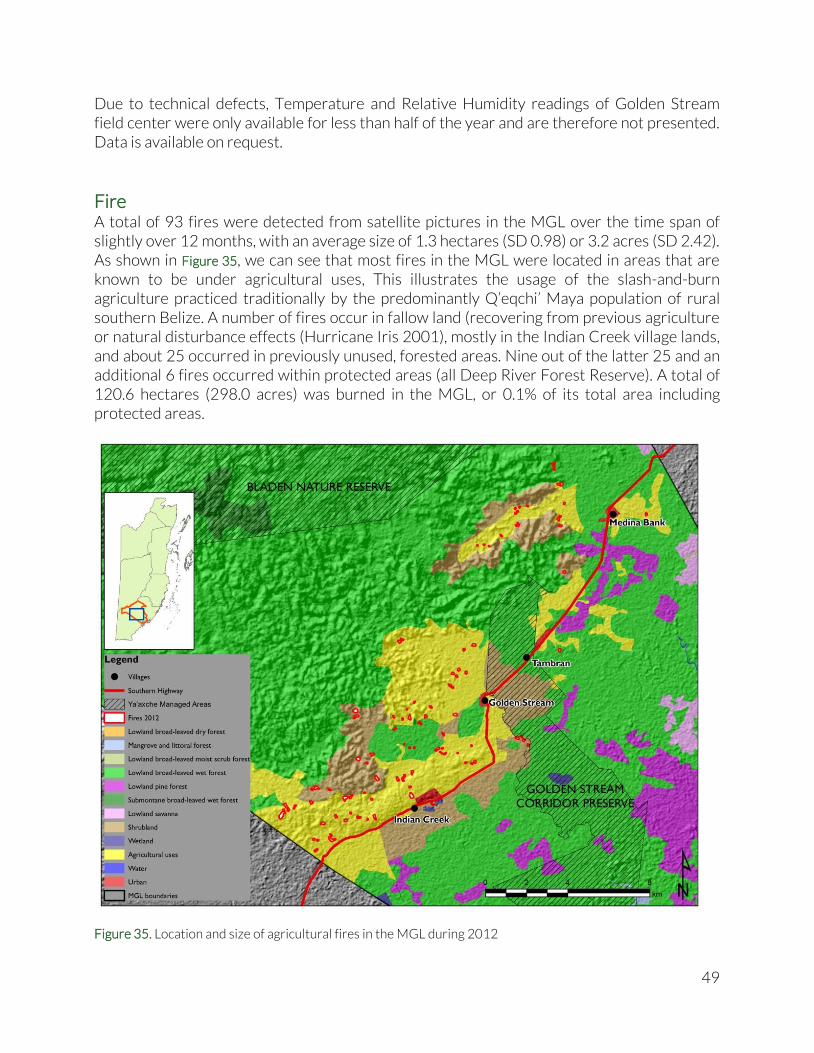
49

Due to technical defects, Temperature and Relative Humidity readings of Golden Stream field center were only available for less than half of the year and are therefore not presented. Data is available on request.

Fire A total of 93 fires were detected from satellite pictures in the MGL over the time span of slightly over 12 months, with an average size of 1.3 hectares (SD 0.98) or 3.2 acres (SD 2.42). As shown in Figure 35, we can see that most fires in the MGL were located in areas that are known to be under agricultural uses, This illustrates the usage of the slash-and-burn agriculture practiced traditionally by the predominantly Q’eqchi’ Maya population of rural southern Belize. A number of fires occur in fallow land (recovering from previous agriculture or natural disturbance effects (Hurricane Iris 2001), mostly in the Indian Creek village lands, and about 25 occurred in previously unused, forested areas. Nine out of the latter 25 and an additional 6 fires occurred within protected areas (all Deep River Forest Reserve). A total of 120.6 hectares (298.0 acres) was burned in the MGL, or 0.1% of its total area including protected areas.

Figure 35. Location and size of agricultural fires in the MGL during 2012

50

Conclusions Throughout the years, we have seen many successes, but also detected several areas in need of improvement. We believe these areas of improvement are an inevitable characteristic of a monitoring scheme in full development. Over the last three years, we have seen a steady increase in biodiversity monitoring effort. The transect monitoring effort has stepped up from 49 to 141km of transect walked during the year, and a suite of additional components has been added to the programme. Some of these components, such as the bat monitoring, tie in with our monthly schedule, but not all of the additions are even an annually recurring effort, e.g. the vegetation plots will be revisited only in 2017, and the snail plots in 2015. The time interval for some of these monitoring efforts will hopefully allow us the time to train young Belizeans in these field techniques and data handling skills needed for the continuation of the monitoring programme at Ya’axché. Birds – We have seen that more of our target species are found in forests than in village land. Particularly the transects in CRFR seem to hold high diversity. The wildlife sightings recorded on patrols and the camera trapping data indicate the presence of game species in GSCP, but remarkably no game species were detected on the village lands transect. However, the flock of Crested guans crossing northwards through Indian Creek is an indication that some game birds are still passing through. Migratory route health indicators seem to be as diverse in both forests and village lands, although the generally increased detectablility in the more open landscape of the village could cause bird numbers to be inflated. Over the years, species richness has increased and so has the proportion of Migratory route health indicators among all observed birds, whereas the proportion of Disturbance indicators decreased. We are careful not to interpret these observations as a sign of increased habitat quality, because we cannot exclude the increased skill level of our field staff, the increased supervision and the improved data entry systems as contributing factors. Large mammals – As in birds, we notice that more target species are detected in the forest, and on average the forest transects hold more diversity than the savannah, which in turn is more diverse than the village lands. The difference is most notable in the proportion of Forest health indicators that drops significantly on the village lands: only a small number of one species (Jaguar) was observed. As opposed to the game birds, the village lands showed a very high proportion of game mammals, which was mostly due to an unusual concentration of Agouti and a high encounter rate of Nine-banded armadillo. Nine-banded armadillo has appeared to be not uncommon in more disturbed areas according to our previous Biodiversity Synthesis Reports, and speculatively might present a case of the ‘meso-predator release effect’, where the lower densities of armadillo predators (e.g. larger cat species) due to human disturbance, releases predation pressure on armadillos and allows their population size (and thus encounter rate) to increase. Popular Game species such as Collared peccary and Paca have lower encounter rates on the village lands than in the forest. Over the last three years, BNR, CRFR and GSCP seem to be well-matched in terms of species richness, and the corridor function of the Golden Stream Corridor Preserve and wider area is illustrated by the species that were seen crossing or were found dead along the roadside (with an average of 23 vehicles passing through every daytime hour). The camera trapping

51

data even showed more species detected in GSCP than in BNR, but taking in to account the reduced trapping effort in BNR we are tempted to say that the data does not contradict the similar mammal diversity of BNR and GSCP. A slight downward trend in the proportion of Forest health indicators was apparent over the last three years (with White-lipped peccary showing the steepest decrease in encounter rate). Although previous years showed a more erratic pattern, this is a trend that needs to be watched closely in the coming years. Bats – Similar to 2011, the savannah seemed to attract much higher species diversity than the forests in CRFR. The top three species with highest AI% in the savannah were the same in both years, however some less common species that were recorded last year were absent during 2012 (Southern and Northern yellow bats). One species was detected in 2012 that was not detected in 2011 (Black-winged little yellow bat). The data from CRFR this year are very similar in terms of species richness and composition to the GSCP data from 2011. With the exception of the very high AI% of Common moustached bats around the Foothills cave in GSCP, the AI% values are roughly comparable as well. In both years, species richness and AI% has proven to be very variable over short distances. This could be due to the ephemeral nature of bat activity as they move between foraging spots throughout the night. Higher diversity and AI% in the savannah could potentially indicate a good feeding ground for bats that are actually roosting much more dispersed in the forests and caves in the wider area. Snails – Early in 2012 two Ya’axché rangers, the Protected Areas Manager and the Research Coordinator were trained for two days in snail sampling techniques and species identification by Dan Dourson, snail specialist in Belize (and former resident biologist at the Belize Foundation for Research and Environmental Education – BFREE) and by Dr. Ron Caldwell, Professor at the Lincoln Memorial University in Tennessee (USA), and director of the associated Cumberland Mountain Research Center. The rangers were then trained by the Research Coordinator in the actual establishment of the monitoring plots. The effort of establishing six plots has been fruitful in terms of skills acquired and lessons learnt. It has yielded a good amount of data, which is unfortunately not yet of sufficient quality to be used in our long-term monitoring programme. The recommendations in the next section will highlight how the data can be used in the future. Vegetation – Although data analyses are incomplete, the results from the slope plot would appear to support the conclusions of Brewer and Webb (2002) that BNR has unusually high tree species richness for northern Central America. Weather – The steadily improving accuracy and consistency of the data collection from the manual weather stations will lead to much more valuable data in the near future. We also expect a lot from the automated weather stations deployed in the Bladen Nature Reserve. Fire – The dry season in 2012 was notably short and wet, which led to very few escaped fires, if any. Most fires seem to have impacted previously cleared land, and only a small proportion of fires seems to have been lit in forested areas and/or protected areas. The risk for escaped

52

fires is heavily dependent on the weather circumstances, and therefore very variable over the years. With the last three Annual Biodiversity Synthesis Reports and the trend analysis in this report, we hope to have confirmed our ability to maintain and develop a biodiversity monitoring programme, and to have established a solid baseline for a set of valuable indicators. In the long run, this should enable us to detect the impacts of future developments on the environment in the Maya Golden Landscape. And beyond, because we shouldn’t forget that these baselines can also be used for comparable forest systems around the Maya Golden Landscape, such as Maya Mountain North Forest Reserve and the remnant forest patches on the community lands of southern Toledo.

53

Recommendations At Ya’axché, we are very much aware that a biodiversity monitoring programme is never really completed. Priority species for conservation, field methods, analysis techniques and financial and human resources are subject to continuous change, and limitations and opportunities can arise or vanish unexpectedly. Nonetheless the Biodiversity Research, Inventory and Monitoring strategy shows a determination and commitment to long-term monitoring activities, which can always be adapted and improved. Birds and large mammals – The gathered transect data is much more detailed and can be used for additional analysis, such as individual species trends in encounter rates, both spatial and temporal trends, modelling of factors that could influence presence/absence or number of individuals for certain species (weather, observer, time of the day, etc), or factors that could influence the number of species detected at a certain time of the year or geographical area. Bats – The strong variation in species richness and AI% over short distances indicates a need to have much more sample locations per area to get a representative image of the diversity in different protected areas. However, in our long term monitoring programme it is unlikely we will be able to achieve sufficient density of sample points for this purpose. Instead, we should aim to expand the number of sample site only slightly but endeavour to go back frequently to this limited set of points over many years, while keeping an eye on environmental changes in the surroundings. Additionally, the variation between sites would warrant site-specific data presentation, rather than pooled together per protected area. Additionally, sporadic harp trapping or mist-netting in the same area has shown presence of species that are not readily detected by the Anabat system. It might be useful to investigate the possibility to include other detection methods to the bat monitoring component. Due to the larger effort and time needed for these methods, this type of monitoring would necessarily need longer intervals between monitoring events. Snails – In conclusion we can say that all necessary skills are in place, with the exception of the species identification. Either we could hire the expert to do the species identification for us, or a more long term sustainable approach would be to hire the expert to conduct a number of specific training sessions in the identification of snails, if necessary only to genus level. An additional recommendation is to design a data management system based on a database application (MS Access, MySQL, etc.) instead of a compilation of spreadsheets to allow for easier extraction of data at different taxonomic levels (species vs. Family) and sample levels (point vs plot). Vegetation – Data collected from the two new PSP’s in 2012 / 2013 will enable us to establish a baseline for long-term monitoring. It is recommended that plots are re-visited every 5 years – i.e. all stems are re-measured, and new recruits (stems that have reached =>5cm DBH) are tagged and measured. If possible, Dr. Brewer’s two existing PSP’s should be re-measured in early 2014 so that new data can be included for analyses. The value of the

54

pristine Bladen Nature Reserve for botanical conservation is clear. However, another massive opportunity to gather information on vegetation (particularly tree species succession), soil and nutrient cycling exists in the Golden Stream Corridor Preserve. The area was strongly impacted by hurricane Iris (Cat.4) in 2001, after which it was left to recover under virtually undisturbed natural circumstances. The natural processes have reshaped the GSCP over the past 11 years to a forest in full recovery. Keeping track of these same processes could yield a treasure of ecological information that could be used to improve the management of this and similar protected areas. Weather – It is recommended that the weather data recording at the manual stations is more closely supervised by a qualified staff member in order to ensure complete and correct data entry. Additional training will have to be provided on the extraction of data from the automated weather station sin BNR. Besides the logical step to provide the obtained data to the National Meteorological Service of Belize once data quality and quantity has sufficiently improved, we are looking at ways to integrate rainfall data with agricultural yield data, which will be arising as a result of data recording courses given at Ya’axché’s Farmer Field school in the coming years. Fire – An interesting step forward will be the continuation of quantifying number and extent of fires that happened in protected areas, and differentiating between fires that happened on previously cleared lands and forested lands. The extent and direction of each fire can be used as an indication of whether it was a controlled or an escaped fire. Over the years, it would be interesting to see the correlation between the number of escaped fires and the weather data for the dry season. Given our previous involvement in research on freshwater invertebrates and their priority status as indicators of freshwater quality in the National Biodiversity Monitoring Program, we are preparing to include freshwater invertebrate monitoring in our schedule using tools developed by our freshwater ecologist, Rachael Carrie. These tools will hopefully not only be used by our rangers, but will be taught at the planned National Ranger Training Academy. The National Ranger Training Academy will be located at Ya’axché’s Golden Stream Field Center and is expected to train protected area rangers from all over Belize in enforcement, environmental law, biodiversity monitoring and other topics to build a pool of top-notch Belizean rangers that care for the environment and natural resources in our beloved country.

55

Acknowledgements To the numerous organisations and persons that have contributed to this piece of work, we are extremely grateful. We cannot list the numbers that have contributed to this area of work at Ya’axché, but we attempt a list of the main supporters and contributors, in no particular order: The Neotropical Migratory Birds Conservation Act of the US Fish and Wildlife Service The Protected Areas Conservation Trust (PACT) PACT Foundation BFREE Dr. Steven Brewer Dr. Ron Caldwell at Lincoln Memorial University – Cumberland Mountain Research

Centre Dan Dourson IdeaWild Dr. Bruce Miller Shajini Jeganmohan Matthew Steinwurtzel We are looking forward to keep developing collaborations and partnerships in the future.

56

References

Acock, M.C. & Pachepsky, Y.A., 1999. Estimating Missing Weather Data for Agricultural Simulations Using Group Method of Data Handling. Journal of Applied Meteorology1, 39, pp.1176–1184.

BFREE/Ya’axché Conservation Trust, 2013. http://www.enn.com/press_releases/4195, visited on 26/10/2013

Brewer, S.W. & Webb, M.A.H., 2002. A seasonal evergreen forest in Belize: unusually high tree species richness for northern Central America. Botanical Journal of the Linnean Society, 138, pp.275–296.

Condit, R., 1998. Tropical Forest Census Plots, Berlin: Springer-Verlag.

Douglas, D., 2011. Land snail species diversity and composition between different forest disturbance regimes in central and eastern Kentucky Forests. Eastern Kentucky University.

Gotelli, N. & Colwell, R., 2001. Quantifying biodiversity: procedures and pitfalls in the measurement and comparison of species richness. Ecology letters, 4, pp.379–391.

Hammer, Ø., Harper, D.A.T. & Ryan, P.D., 2001. PAST: Paleontological Statistics package for education and data analysis. Paleontologia electronica, 4(1), p.9.

Hill, M.O. & Mar, N., 1973. Diversity and evenness: a unifying notation and its consequences. Ecology, 54(2), pp.427–432.

Hofman, M., 2012. 2010 Biodiversity Synthesis Report, Ya’axché Conservation Trust, Punta Gorda, Belize, Central America.

Hofman, M.P., Ack, M. & McLoughlin, L., 2013. Biodiversity Synthesis Report 2011, Ya’axché Conservation Trust, Punta Gorda, Belize, Central America.

Jones, H.L. & Gardner, D., 2003. Birds of Belize, Austin, Texas, USA: University of Texas Press.

Jost, L., 2010. The Relation between Evenness and Diversity. Diversity, 2(2), pp.207–232.

Magurran, A.E., 2004. Measuring Biological Diversity, Oxford, UK: Blackwell Publishing, Ltd.

Miller, B.W., 2001. A method for determining relative activity of free flying bats using a new activity index for acoustic monitoring. Acta Chiropterologica, 3(1), pp.93–105.

Lo Presti, R., Barca, E. & Passarella, G., 2010. A methodology for treating missing data applied to daily rainfall data in the Candelaro River Basin (Italy). Environmental Monitoring and Assessment, 160(1-4), pp.1–22.

57

Reid, F.A., 2009. A field guide to the mammals of Central America and Southern Mexico 2nd ed., USA: Oxford University Press.

Rényi, A., 1961. On measures of entropy and information. In J. Neyman, ed. Fourth Berkeley Symposium on Mathematical Statistics and Probability. Berkeley, CA, USA: University of California Press, pp. 547–561.

Ruscalleda, J., 2011. Land Use / Land Cover Change in the Maya Golden Landscape  : 1980-2010,

Ruscalleda, J., 2012. Land Use/Land Cover Change in the Maya Golden Landscape: 1980-2012, Punta Gorda, Belize, Central America.

Shimek, B., 1930. Land snails as indicators of ecological conditions. Ecology, 11(4), pp.673–686.

Tóthmérész, B., 1995. Comparison of different methods for diversity ordering. Journal of Vegetation Science, 6(2), pp.283–290.