1

The Ozarks Environmental and Water Resources Institute (OEWRI) Missouri State University (MSU)

Big River Mining Sediment Assessment Project

Big River Borrow Pit Monitoring Project

FINAL REPORT

Field work completed Summer 2009 to Spring 2010

Prepared by:

Marc R. Owen, M.S., Research Specialist II Robert T. Pavlowsky, Ph.D., Director and Principal Investigator

Derek J. Martin, M.S., Research Specialist I

Ozarks Environmental and Water Resources Institute Missouri State University

901 South National Avenue Springfield, MO 65897

bobpavlowsky@missouristate.edu

Funded by: U.S. Fish and Wildlife Service

Cooperative Ecosystems Studies Unit

David E. Mosby, Environmental Contaminants Specialist Columbia Missouri Field Office

573-234-2132 Ext. 113 Dave_Mosby@fws.gov

May 24, 2012

OEWRI EDR-10-003

2

TABLE OF CONTENTS

TABLE OF CONTENTS ............................................................................................................................ 2 LIST OF TABLES ...................................................................................................................................... 3 LIST OF FIGURES .................................................................................................................................... 3 ABSTRACT ................................................................................................................................................ 5 INTRODUCTION ...................................................................................................................................... 6 STUDY AREA ........................................................................................................................................... 7

Physiographic Setting .............................................................................................................................. 7 Borrow Sites ............................................................................................................................................ 7

METHODS ................................................................................................................................................. 9 Sediment Excavation ............................................................................................................................... 9 Volume Estimates ................................................................................................................................... 9

Survey Methods ................................................................................................................................... 9 Topographic Analysis .......................................................................................................................... 9 Gravel Bulk Density and Volume Conversions ................................................................................ 10

Sediment Analysis ................................................................................................................................. 10 Flood Hydrographs ................................................................................................................................ 11

Drainage Area-Discharge Relationships ........................................................................................... 11 Drainage Area-Duration Relationships ............................................................................................. 11

Bed Load Transport Rate ...................................................................................................................... 12 BAGS Model Data Input ................................................................................................................... 13

RESULTS AND DISCUSSION ............................................................................................................... 15 Flood Records and Hydrology .............................................................................................................. 15 Survey Results and Volume Estimates.................................................................................................. 15

Bone Hole .......................................................................................................................................... 15 Bar Site .............................................................................................................................................. 17 Comparison of Low Dam and Bar Sites ............................................................................................ 20

Sediment Texture and Geochemistry .................................................................................................... 20 Bone Hole .......................................................................................................................................... 20 Bar Site .............................................................................................................................................. 22

Flood Hydrographs ................................................................................................................................ 22 Bed Load Transport ............................................................................................................................... 23

Cross-Section Survey ........................................................................................................................ 23 Slope .................................................................................................................................................. 23 Channel Sediment Size ...................................................................................................................... 23 Manning’s n ....................................................................................................................................... 24 Bedload Transport Model .................................................................................................................. 24 Event Bedload Transport ................................................................................................................... 24

Environmental Restoration Implications ............................................................................................... 25 Bedload Transport Rates and Recovery Times ................................................................................. 25 Available Storage .............................................................................................................................. 26 Channel Dredging vs. Bar Skimming ................................................................................................ 26

3

Excavation Schedule and Effectiveness ............................................................................................ 27 Additional Geomorphic Information ................................................................................................. 27

CONCLUSIONS AND RECOMMENDATIONS ................................................................................... 28 LITERATURE CITED ............................................................................................................................. 30 TABLES ................................................................................................................................................... 34 FIGURES .................................................................................................................................................. 40 APPENDIX A – Flood Frequency Data ................................................................................................... 58 APPENDIX B – Survey Maps .................................................................................................................. 61 APPENDIX C – Volume Changes by Survey .......................................................................................... 69 APPENDIX D – Sediment Sample Data .................................................................................................. 70 APPENDIX E – Sediment Sample Locations .......................................................................................... 72 APPENDIX F – Pebble Count Data ......................................................................................................... 73 APPENDIX G – Cross-section Data ........................................................................................................ 74 APPENDIX H – BAGS Model Output..................................................................................................... 75 APPENDIX I –Site Photographs .............................................................................................................. 76

LIST OF TABLES

Table 1. Explanation of Geologic Units .................................................................................................. 34 Table 2. USGS Real-Time Gages Used for this Study ............................................................................. 34 Table 3. Sediment Sample Analysis Statistics at the Bone Hole ............................................................. 35 Table 4. Sediment Sample Analysis Statistics at the Bar Site ................................................................. 36 Table 5. Flood Frequency Data Used to Estimate Discharge at the Bar Site ........................................... 37 Table 6. Flood Duration Data used to Estimate Duration at the Bar Site ................................................. 37 Table 7. Channel Geometry at Key Locations on the Cross-Section ....................................................... 37 Table 8. Grain-Size Distribution Based on Pebble Counts ...................................................................... 38 Table 9. Bedload Rating Table (active bed = 36 m) ................................................................................ 38 Table 10. Predicted Maximum Bedload Transport During Monitoring Period ....................................... 39

LIST OF FIGURES Figure 1. Project Location Within the Big River Watershed ................................................................... 40 Figure 2. Bedrock Geology of the Big River Basin ................................................................................. 41 Figure 3. Location of the Borrow Pit Sites Near Desloge. ...................................................................... 42 Figure 4. Bone Hole Site on the Big River Near Desloge, Missouri. ....................................................... 43 Figure 5. Bar Sites on the Big River Near Desloge, Missouri. ................................................................ 44 Figure 6. Downstream Flood Frequency Analysis for Big River Gages. ................................................. 45 Figure 7. Flood Hydrographs Used to Establish Drainage Area-Duration Relationships. ....................... 45 Figure 8. Project Period Rainfall Compared to Historical Rainfall Records From St. Louis, Missouri.. 46 Figure 9. Hydrograph at the Irondale Gage Located 30 km Upstream of the Bar Site With Flood Frequency. ................................................................................................................................................. 46

4

Figure 10. Changes in Bone Hole Cross-Section at Station R-km 165.4 in the A.) Pre-Excavation Survey, B.) Post-Excavation Survey, C.) Post-Flood Survey and D.) Post-Bankfull Survey. ................. 47 Figure 11. Absolute Volume Changes Measured at the Bone Hole Relative to Pre-Excavation Condition................................................................................................................................................... 48 Figure 12. Changes at the Bar Head, Cross-Section at Station R-km 163.4 in the A.) Pre-Excavation Survey, B.) Post-Excavation Survey, C.) Post-Flood Survey and D.) Post-Bankfull Survey. ................. 49 Figure 13. Changes at the Bar Middle, Cross-Section at Station R-km 163.4 in the A.) Pre-Excavation Survey, B.) Post-Excavation Survey, C.) Post-Flood Survey and D.) Post-Bankfull Survey. ................. 50 Figure 14. Changes at the Bar Tail, Cross-Section at Station R-km 163.4 in the A.) Pre-Excavation Survey, B.) Post-Excavation Survey, C.) Post-Flood Survey and D.) Post-Bankfull Survey. ................. 51 Figure 15. Absolute Changes in Measured Volume at the Bar Site Relative to Pre-Excavation Condition................................................................................................................................................... 52 Figure 16. Average Particle Size Distribution from Samples Collected From the Bone Hole. ................ 53 Figure 17. Sediment Composition of Samples Collected From the Bone Hole. ..................................... 53 Figure 18. Average Concentration of Metals in Samples Collected From the Bone Hole. ..................... 53 Figure 19. Average Particle-Size Distribution From Samples Collected at the Bar Site. ........................ 54 Figure 20. Sediment Composition of Samples Collected at the Bar Site. ............................................... 54 Figure 21. Average Concentration of Metals in Samples Collected From the Bar Site. ......................... 54 Figure 22. Drainage Area-Duration Relationships the A.) Base and B.) 95% Peak from Hydrographs for Selected Floods at Big River Gages.......................................................................................................... 55 Figure 23. Channel Hydrologic Characteristics at Station R-km 163.4 Near the Bar Site Cross-Section.................................................................................................................................................................... 56 Figure 24. Longitudinal Profile at the Bar Site. ....................................................................................... 56 Figure 25. Grain-Size Distribution at the Bar Site. ................................................................................... 56 Figure 26. Bedload Transport Rating Curve Evaluation A.) Rating Curve and B.) Analysis of Model Fit Comparing Both Full and Partial Datasets................................................................................................ 57

5

ABSTRACT In-channel dredging is a possible strategy for the removal of lead contaminated sediment from the Big River. This project evaluates the feasibility of dredging by testing a borrow pit strategy at two sites along the Big River located near the Desloge tailings pile. The first site is located at what is locally known as the Bone Hole where channel sediment is trapped behind a low-water bridge. The second site is located about 2 km downstream at a natural point bar complex (the Bar Site) that has formed on the inside of a large valley bend. The fieldwork for this project was carried out in the period from October 2009 to March 2010. At each site, a series of four topographic surveys were used to monitor the changes in sediment volume: (i) pre-excavation; (ii) post-excavation of approximately 382 m3 (500 yd3) of sediment; (iii) after a major flood event (>10-year recurrence interval (RI)); and (iv) after several near bankfull events (less than 1.5-year RI). Volume analysis at the Bone Hole showed the excavated pit refilled after the large flood and remained stable after the series of subsequent near bankfull events. The “skimming” of the vegetated center bar near the head of the complex at the Bar Site may have destabilized the bar and made it more sensitive to the influence of a large flood on erosion at the head and middle bar areas. This indicates low-water bridge sites, compared to bar sites, may be the preferred alternative for mine sediment excavation activities. However, this study only evaluated one bar site and more research is needed to examine other bar settings for excavation activities and geomorphic recovery. It appears “cleaner” natural sediment is replacing contaminated sediment at both locations, and Pb and Zn concentrations decreased over the monitoring period at the Bone Hole. However, Pb and Zn concentrations at the Bar Site did not change over the monitoring period. This is likely due to remobilization of stored contaminated sediment at flows required to deposit material on the bar versus the bed at the Bone Hole. The presence of heavily contaminated fine-grained “slime” deposits previously buried by chat sediment should be located and mitigated prior to excavation activities to reduce the risk of remobilization. Bedload transport modeling and field data analysis indicate that re-excavation activities should be repeated annually or immediately after high magnitude overbank flood events to maximize the rate of contaminated sediment removal from the river during the restoration period. However, a two year re-excavation cycle would be more appropriate if the goal is to maximize the amount of sediment removed per excavation event.

6

INTRODUCTION Mining chat and tailings inputs have contaminated channel sediments with lead and other metals in the Big River below Leadwood for more than a century (MDNR, 2007a). The Big River Mining Sediment Assessment Project was implemented in the Fall of 2008 to better understand the spatial distribution of lead (Pb) in channel sediments and floodplain soils and to identify the major storages of mining sediment and Pb in the Big River from Leadwood to its confluence with the Meramec River (Pavlowsky et al., 2010). Several recent studies have confirmed the widespread distribution of in-channel sediment lead concentrations in excess of the aquatic Probable Effects Concentrations (PEC) for Pb of 128 ppm established by MacDonald et al. (2000). It is estimated over 3,600,000 m3 of contaminated channel sediment (i.e., sediments exceeding the PEC) is stored within the lower 171 km of the Big River from Leadwood to the mouth at the confluence with the Meramec River (Pavlowsky et al., 2010). An estimated 1,357,000 m3of contaminated sediment and 2,600 Mg of Pb are stored in channel deposits between river kilometer (R-km) 171 and 118 in St. Francois County based on tile probe depth surveys and XRF analysis of sediments (Pavlowsky et al., 2010). The average volume of stored mining sediment in the Big River segment in St. Francois averages 2,570 +/- 14% (1s) m3/100 m with the upper limit of potential storage at double that amount (Pavlowsky et al., 2010). Concentrations of Pb in the bed and bar deposits typically exceed 1,000 ppm (MDNR, 2007a; Roberts et al., 2009; Pavlowsky et al., 2010). Consequently, mining-related sedimentation and contamination are believed to be responsible for decreased mussel populations and elevated tissue Pb concentrations in aquatic organisms in the Big River in St. Francois County (Buchanon, 1979; Schmitt and Finger, 1982; Schmitt et al., 1987; Roberts and Bruenderman, 2000; Gale et al., 2002; Roberts et al., 2009). The spatial distribution of contaminated channel sediment at the basin-scale is well documented for the Big River (MDNR, 2007a; Roberts et al., 2009; Pavlowsky et al., 2010). Presently, elevated Pb concentrations in the fine sediment fraction (<2 mm in diameter) of bed and bar deposits occur far downstream in the Big River. Sediment-Pb concentrations increase sharply from <50 ppm above Leadwood at river kilometer (R-km) 170 to >1,500 ppm between Desloge (R-km 163) and Bonne Terre (R-km 136). From Bonne Terre, Pb concentrations decrease downstream to about 500 ppm above Mill Creek (R-km 116) at the Jefferson County line and then gradually decrease to about 100 ppm at the Meramec River (R-km 0) (Pavlowsky et al., 2010). In contrast, coarser mining chat particles composed of very fine to fine gravel particles (2 mm to 16 mm diameter) remain in St. Francois County and have not yet been transported out of the mining-affected segment of the Big River (Pavlowsky et al., 2010). While the patterns of sediment-Pb and chat concentrations in the Big River have previously been reported (Pavlowsky et al., 2010), little is known about the actual transport and deposition rates of bed sediment within the Big River and the amounts of sediment moved by high flow and flood events. This information is needed to evaluate the long-term mobility and residence times of contaminated channel sediment in the Big River and to assess the effectiveness of proposed remediation measures on contaminated load reduction. The purpose of this project is to evaluate the feasibility of dredging and removal of in-channel mining sediment for terrestrial disposal as a restoration or remediation strategy to reduce the downstream loading rates of Pb-contaminated sediment for both chat and finer tailings particles in St. Francois County. This pilot study focuses on monitoring the geomorphic behavior and

7

sedimentation rates within previously dredged reaches of the Big River to evaluate the feasibility of using these sites as long-term sediment removal sites. Two common depositional environments in the Big River are evaluated in this report: (i) sub-aqueous sedimentation zone upstream of a low-water bridge and (ii) sub-aerial gravel bar deposit on the inside of a channel bend. The specific objectives of this project are to: (i) use successive topographic surveys of the borrow pit sites to track changes in bed sediment volume over time; (ii) monitor the sedimentary response of the borrow sites in relation to flood events; (iii) monitor the geochemistry of the borrow and fill material over time; and (vi) use channel storage estimates and modeled bedload transport rates to evaluate the frequency of dredging required to meet restoration goals.

STUDY AREA Physiographic Setting The Big River Watershed is located in eastern Missouri and mainly within the Salem Plateau of the Ozarks Highlands, which composes about 68% of the drainage area (Figure 1). The Big River drains about 2,500 km2 before it flows into the Meramec River near Eureka, Missouri along the Central Mississippi Valley. While the headwaters of the river are in the St. Francois Mountains, which are composed of igneous rocks, most of the drainage area of the Big River is underlain by dolomite with some limestone and shale units (Figure 2, Table 1). Sandstones outcrop locally in the southern and northern portions of the basin. The chief host-rock of Pb and Zn mineralization is the Bonne Terre Dolomite of Cambrian age which outcrops at the surface in the southern and eastern portions of the basin (Smith and Schumacher, 1993). Upland soils in the area are typically formed in a thin layer of silty Pleistocene loess overlying cherty or non-cherty residuum formed in dolomite, limestone, and shale (Brown, 1981). The average annual temperature in this area is about 55 oF ranging from an average of 32 oF in January to 77 oF in July (Brown, 1981). The annual rainfall in the region averages about 40 inches with the wettest period in the spring months (Brown, 1981). There are three U.S. Geological Survey discharge gaging stations on the Big River located at the following locations: (1) Irondale (07017200), draining 453 km2 with a mean flow of 5.2 m3/s since 1965; (2) Richwoods (07018100), draining 1,904 km2 with a mean flow of 20 m3/s since 1942; and (3) Byrnesville (07018500), draining 2,375 km2 with a mean flow of 25 m3/s since 1921. Borrow Sites Two sites along the upper portion of the Big River near Desloge, Missouri were chosen to perform the borrow pit study (Figure 3). Each site represents a different type of depositional environment found along the Big River, a low-water bridge and a point bar complex. The sites chosen are located

8

approximately 2 km apart where the Big River flows along the upstream margin of the Desloge tailings pile. This area of the river is located 5.5 km downstream of Eaton Branch that drains the Leadwood tailings pile which has been largely stabilized. Both sites are also located upstream of Flat River Creek which receives tailings inputs from three large mines and may still be providing significant amounts of contaminated sediment to the Big River today (MDNR, 2007b; Pavlowsky et al., 2010). The Bone Hole site contains a channel deposit immediately upstream of a low-water bridge. It is located at R-km 165.3 on a straight section of the river with an exposed valley bluff on the north side, a small tributary entering from the south, and the low-water bridge that crosses the river about 30 m downstream of the tributary mouth (Figure 4). In relation to the lowest elevation of the top of the bridge, the channel bed elevation is nearly level with the top of the bridge deck immediately upstream. Going upstream, the bed elevation is around 0.5 m lower in the center of the excavation area and drops another meter at the tail of the next upstream pool. The banks at this location are about 3.2 m above the lowest elevation on the top of the bridge. Channel reaches immediately upstream of low-water bridges, such as this, and mill dams are typically zones of channel sediment deposition because the flow is obstructed, local slope is lowered, and sediment transport rates decrease (Knighton, 1998). Therefore, areas above dams could make good locations for sediment borrow sites that will provide for the long-term trapping and periodic removal of mining sediment. Aerial photographs of the area show the low-water bridge was built sometime between 1937 and 1954. Bridge construction appears to have caused erosion along the right bank downstream of the bridge and the channel has shifted south. Upstream of the bridge the channel may be wider than in 1937, however the channel planform appears to have remained stationary since 1937. The Bar Site is located about 2 km downstream from the Bone Hole site at R-km 163.4. Excavation activities focused on the removal of contaminated sediment from the head and mid area of a point bar complex located on the inside of an easterly bend of the Big River (Figure 5). The Bar Site is located on the northwest side of the Desloge tailings pile within a confined valley meander that flows around the tailings disposal area at Desloge. Here, the channel flows along a bedrock bluff at the valley margin that is prohibiting further lateral migration to the northeast. The point bar complex consists of both a high bar and a vegetated center bar separated by a chute channel. Point bars typically form on the inside of a meander bend of the river where the velocity gradient of water flowing around a bend is lowest (Leopold et al., 1964). The top of the high bar is about 2 m higher than the deepest part of the channel. The top of the bank is around 4.5 m above deepest part of the channel. In addition, the head or upstream end of the bar tends to contain relatively coarse bed sediment since it is a primary location for energy dissipation in the channel and sometimes forms the core of a riffle crest (Knighton, 1998). Sediment size tends to decrease downstream along a point bar from head to tail (Rosgen, 1996). The Bar Site reach exhibits some geomorphic characteristics of a discrete sedimentation or disturbance zone found along Ozark rivers (Saucier, 1983; McKenney et al., 1995; Jacobson and Gran, 1999). The point bar complex accumulates gravel during high flows as hydraulic forces are enhanced where the channel meets the valley wall and field observations indicate that deposition and erosion patterns vary within bar head, tail, and chute areas in response to flood events. However, historical aerial photographs indicate that the thalwag or deepest thread of the channel has not shifted much over the past 50 years and that the majority of the present bar has been in place for some time. This condition is further supported by the

9

occurrence of Sycamore and Black Willow trees (up to 4” in diameter at breast height) growing in bar deposits along the edge of the low-flow channel margin, covering about 20% of the total bar area, at the time of the pre-excavation survey (July 2009) .

METHODS

Sediment Excavation HydroGeologic, Inc. (HGL) was contracted to perform the borrow pit excavations. HGL was permitted to excavate 382 m3 (500 yds3) of material from each location in compliance with approved procedures and quality assurance measures. On October 5, 2009 HGL oversaw the excavation activities at the Bar Site (HGL, 2009). Excavation focused on the upstream half of the bar complex, essentially leveling the bar from its highest point, to the water line. On October 6, 2009 HGL oversaw the excavation of sediment from the site Bone Hole directly upstream of the low-water bridge (HGL, 2009). The excavator was positioned in the center of the channel and dug a pit that nearly spanned the channel. The extent of the excavation was marked so an accurate survey could be performed in the part of the channel that was excavated. Volume Estimates Changes in sediment volume were calculated using GIS-based analysis of changes in digital elevation models (DEM) created from a series of topographic surveys of the borrow sites prior to excavation, after excavation, and following several flood events. The following describes survey methods, DEM creation, and GIS based cut/fill analysis techniques. Survey Methods Topographic surveys were performed using a Topcon GTS-225 electronic total station and a Tripod Data Systems (TDS) Ranger data collector and Survey Pro software (OEWRI, 2007a; TDS, 2000). Each successive survey was referenced to the same permanent benchmark. Benchmark coordinates were collected using Topcon HiPerLite dual frequency base station global positioning system (GPS) (Topcon, 2004). The Bone Hole site survey consisted of six channel cross-sections that spanned the area of the proposed excavation. Cross-sections were spaced 10 meters apart and elevations within the cross-section were collected approximately every five meters across the channel. Additional points were surveyed between cross-sections to increase survey point density which helped create more accurate DEM. The bar site survey consisted of 17 channel cross-section surveys spanning the entire bar where the proposed excavation would take place. Cross-sections were spaced 10 meters apart and elevations were collected approximately every two meters across the channel. Cross-sections and longitudinal profile surveys were also collected for the purposes of developing stage-discharge rating curves for the Bar Site to provide information needed for bedload transport modeling. Topographic Analysis Location data collected at the benchmarks were processed using Topcon Link software and sent to NOAA’s Online Positioning User Service (OPUS) for post-processing in the NAD 83 State Plane (feet)

10

Missouri East coordinate system. Benchmark coordinates were used to orient topographic surveys to MO EAST State Plane coordinates using Foresight DXM software (TDS, 2003). Corrected survey points were imported into ESRI ArcGIS software for topographic analysis. Using the ESRI ArcGIS Spatial Analyst extension, survey points were used to create a Triangulated Irregular Network (TIN) surface. These data were transformed into a 0.71 m x 0.71 m cell digital elevation model (DEM) and “smoothed” with neighborhood statistics using mean values of a 3 x 3 cell moving window. Topographic changes between surveys were calculated by measuring the volume changes in the DEM surface from a specified elevation down to the lowest elevation for each survey using the “Area and Volume Statistics” tool in ESRI’s ArcGIS 3D Analyst extension. Gravel Bulk Density and Volume Conversions Bulk density values for gravel reported by various on-line references range from 1.5 for loose, dry gravel to 1.9 for natural gravel and sand (www.simetric.co.uk/si_materials.htm). For this study, the bulk density of gravel deposits in the Big River is assumed to be 1.8 Mg/m3 (Napolitano, 1996; Lisle and Napolitano, 1998). Volumetric changes in gravel deposits are converted to mass unit by multiplying by the bulk density. Bed sediment loads are converted to their representative volume within a bar or bed deposit by dividing the transport mass by the bulk density of the gravel. Sediment Analysis Bed and bar sediment samples were collected during each of the survey periods and represented different depositional environments at the site. Samples at the Bone Hole site were collected within the wetted portion of the channel with a slotted shovel to a depth of 20 cm in the area of sediment accumulation upstream of the low-water bridge and along the margins of the borrow pit area. Samples at the bar complex were collected above the water line from 10 to 20 cm below the bar surface at locations representing the range of surface elevations and features present. The number and location of sediment samples collected during each of the survey periods varied, but were distributed within the borrow area and adjacent bed and bar surfaces. Samples were stored in plastic bags, oven dried at 60 oC, and disaggregated with mortar and pestle. Gravimetric textural analysis was completed on size fractions produced by hand sieving. Grain counts of the 4 mm to 8 mm chat-sized fraction were used to sort the grains into different mineral types for source evaluation. The composition of the chat-size material (i.e. 4-8 mm grains) is a good indicator of the source of the material. Channel sediment rich in dolomite chips indicates a mining source while the presence of weathered chert and quartz grains is attributed to natural sources (Wronkiewicz et al., 2006; Pavlowsky et al., 2010). Shale flakes are also an indicator of mill crushing but are not found in great abundance. As described here, “slag” grain counts probably include coal chips and ash cinders from railroad and industrial furnace sources as well as residual slag created by the foundary works and mill roasters used in association with the mining activities in the region. X-ray Fluorescence (XRF) analysis was used in the OEWRI laboratory to determine the geochemistry of sediment samples, similar to the analytical technology used in prior Big River studies (MDNR, 2001, 2003, 2007b; Roberts et al. 2009). In the present study, an Oxford Instruments X-MET 3000 TXS+ was

11

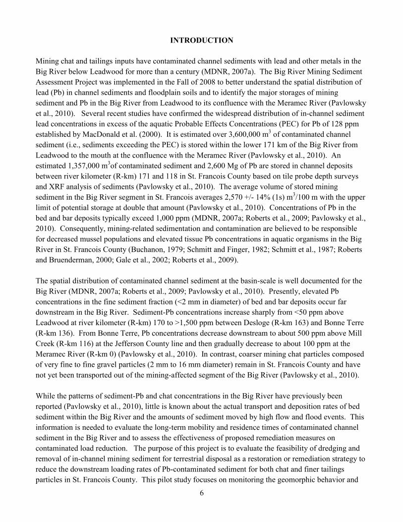
used to determine the concentrations of Pb, Zn, Fe, Mn, and Ca in channel sediment samples. The elements with the highest analytical resolution on the XRF unit include Pb, Zn, copper (Cu), titanium (Ti), iron (Fe), selenium (Se), and calcium (Ca). The standard operating procedure (SOP) for use of the XRF in the OEWRI laboratory can be found at http://oewri.missouristate.edu/ (OEWRI 2007b). Standard checks and duplicate analyses are routinely used every 10 to 20 samples with relative difference values for duplicates generally less than 10%. Flood Hydrographs Flood hydrographs were developed to evaluate the magnitude-frequency relationships for the high in-channel flows and floods that occurred during the study period. Two methods were used for this purpose: (i) Drainage area-discharge relationships between available flow gages on the Big River and the ungaged Bar Site and (ii) Drainage area-duration relationships between available flow gages on the Big River and the ungaged Bar Site. Drainage Area-Discharge Relationships The study sites are located between three U.S. Geological Survey (USGS) real-time gage stations at Irondale, Missouri (Big River at Irondale #07017200), Richwoods, Missouri (Big River near Richwoods #07018100), and Byrnesville, Missouri (Big River near Byrnesville #07018500) with all gages having >45 years of record (Table 2). Drainage area-discharge relationships were analyzed using both flood frequency and flow frequency curves. Flood frequency was calculated using the ranked maximum annual peak discharge from 1965-2010 at all three gages with the following equation (Knighton, 1998): T = (n-1) / N T = return interval (years) n = number of years of record N = rank of a particular event Flood frequency was estimated for the Bar Site using regression equations based on interval discharges and drainage area relationships at the three USGS gages for the 1.5-yr, 2-yr, 5-yr, and 10-yr floods (Figure 6). Drainage Area-Duration Relationships Hydrographs for three of the floods to be analyzed were created for the March 25, 2010, October 22-23, 2009, and October 29, 2009 flood events at each gaging station on the Big River (Figure 7). Duration was calculated at the base flow and 95% peak flow of the hydrograph at each gage. Duration at the Bar Site was estimated using regression equations based on duration and drainage area relationships for each of the events representing the range in magnitude of events that occurred during the monitoring period. Drainage area-corrected hydrographs for duration and discharge were used in combination with a bedload transport model to estimate sediment transport rates at the Bar Site to provide an independent comparison with field survey observations.

12

Bed Load Transport Rate

Bed load transport was calculated using the Bedload Assessment for Gravel-bed Streams (BAGS) software developed by the U.S. Forest Service (http://www.stream.fs.fed.us/publications/bags.html) (Pitlick et al., 2009; Wilcock et al., 2009). BAGS uses the channel cross-section and the grain-size distribution along the bed in user-defined equations that are based on the size of the material in the channel and the method used to collect these data. The Wilcock and Crowe (2003) equation was chosen for this project because surface grain-size distribution is available and there is >5% sand in the bed (Appendix F; Wilcock et al., 2009). A bed load rating curve was developed and combined with the Bar Site hydrograph to estimate the maximum potential bed load (Mg) for the storm events that occurred during the monitoring period. Typically, only a portion of the bed material is mobile during a flood event and this phenomenon is described as partial transport (Wilcock et al., 2009). Partial transport can also vary by particle size, having a greater percentage of sand size particles mobile versus a lower percentage in the gravel size class. The BAGS model reports fractional transport rates by different bed material size classes. The BAGS model calculates the maximum bed load capacity of the channel assuming that sediment supply is not limited. However, both sediment supply and the width of channel actively transporting sediment may vary greatly within a reach over the course of a flood event (Wilcock et al., 2009). At the Bar Site, field evidence of active bar surface transport after high flow and flood events suggest that the entire wetted bed of the river is rarely entirely active. Little change occurs in some areas, painted sediment particle “tracers” remain in pre-storm positions at times, and local variations in structure caused by vegetation, large woody debris, bed patch variations, and narrow channels on the bar surface can reduce or increase the chances for transport accordingly (Ferguson. 2003). At flows near the critical discharge for bed transport, probably less than 5% of the bed width is transporting bed load at any given moment (Ashmore et al., 2011). Around bankfull discharge, only about 20 to 30% of the wetted bed width might be active (Ashmore et al., 2011). However, during floods with >5-yr RI, it is reasonable to expect that 100% of the bed width is actively transporting sediment (Wilcock et al., 2009). Indeed, at the Bar Site after a large flood, a sand splay about 1,000 m2 in area was deposited on the floodplain along the inside of the bend suggesting that the sand transport occurred across the entire bed and inundated bar area during the flood. In this study, the discharge-active width trend described above will be applied to the bed load transport modeling results of this study to evaluate the sensitivity of bedload transport calculations to the effects of partial transport. The bedload transport modeling and analysis presented in this report is used as an independent check on the field data collected to determine the rates and flow conditions at which the borrow pits will fill in with sediment and become ready for another excavation cycle. The results generated, if judged to be valid, can be used to address questions during the mitigation planning process. However, it is well recognized that errors in bedload modeling results can exceed an order of magnitude or more and this fact is acknowledged and critically addressed by the bedload experts who developed the BAGS model (Pitlick et al., 2009; Wilcock et al., 2009). Problems occur due to parameter estimation, lack of gage data for flow calibration, limited sediment data, local variations in slope, uncertainty in active width, and fluctuation in bed configuration and sediment transport at a scale of <30 m2 (Ferguson, 2003; Recking,

13

2010; Ashmore et al., 2011). While field measurements of bed load transport can be used to calibrate models, field results can also be affected by errors of over an order of magnitude even if collected at the same location (Pitlick et al., 2009). Moreover, sampling of bedload transport during bankfull or larger floods would be very difficult, impractical, and beyond the scope of this study. Nevertheless, this sediment transport analysis attempts to understand the overall behavior of the Big River in the vicinity of the two project sites. The channel reach used for modeling purposes in this study has characteristics that improve the chances of an accurate BAGS model including a relatively straight channel, that is not braided(along the upper 2/3 of the reach), and a fairly uniform slope (Pitlick et al., 2009) BAGS Model Data Input The BAGS model requires the user to input the channel cross-section, slope, Manning’s roughness coefficient, and bed sediment size distribution of the reach. Methods and explanation of each input is detailed here: Cross-sectional survey The cross-sectional survey entered into BAGS was collected at approximately R-km 164.4 at the Bar Site using the same survey procedures and equipment outlined above. This transects spans the bar head and includes the total in-channel area, or bankfull stage, the terrace, and the high water mark from the flood on October 30, 2009. Channel area and width were also calculated separately using Intelisolve’s Hydraflow Express software (Intelisolve, 2006). Channel Slope Channel slope is a primary variable required for hydraulic analysis. Slope values for this study were determined from available topographic maps, digital elevation model data, and longitudinal surveys from the field sites (Rosgen, 1996). Channel slope values determined from topographic maps using contour line measurements are similar to field slopes at near-bankfull discharges since variations in local channel topography are evened or “washed” out (Magilligan, 1988; Knighton, 1998). The bedload model (BAGS) used in this study accepts one of three slope values: reach average water slope, reach average channel bed slope, and friction or energy slope for a computer model (Pitlick et al., 2009). For the best model results, the channel slope should be calculated for a relatively long reach that includes several pool riffle sequences (Pitlick et al., 2009). Manning’s Roughness Coefficient Manning’s equation requires a roughness coefficient (n) value that is estimated in this protocol using a field-based method. This protocol estimates Manning’s n using sinuosity, median grain size, and mean residual pool depth to account for channel irregularities due to planform pattern, bed sediment size, and bed form topography (French, 1985, Pizzuto et al, 2000, Martin, 2001). Manning’s roughness coefficient (n) was calculated using the following equation:

n = Fp (ng + nb) + ng + nb

Fp = Channel form roughness = 0.6 (K-1) ng = 0.0395 (D50)1/6

14

nb = 0.02 (drp/ dbf) , note: nb = 0.02 for values > 0.02) K = sinuosity (reach length/valley length (m/m)) D50 = median grain size of the bed (m) dbf = mean bankfull depth (m) drp = mean residual pool depth of the entire active channel area (m) Channel form roughness (Fp) is calculated using the sinuosity factor with sinuosity (K) determined by dividing reach length along the thalweg by the “straight line” valley length measured from aerial photography or topographic map. Grain or particle roughness (ng) is accounted for in the equation by using the median (D50) grain size diameter from pebble count surveys (Chang, 1988). The bed form roughness resistance factor (nb) is the ratio between the mean residual pool depth (drp) of the reach and the mean bankfull depth (dbf). Bed Material Size The diameter of bed and bar substrate is routinely measured using some variation of the Wolman pebble count method (Wolman, 1954). Pebble counts involve measuring the B- or intermediate-axis of 100 to 400 individual bed particles collected from the channel bed by using a ruler or template (Bunte and Abt, 2001). Stratification of the reach by channel unit or bed form during pebble counting can reduce errors introduced by mixed populations and variable bed form scale (Buffington and Montgomery, 1999; Kondolf et al., 2003). In this study, four channel units were sampled individually including the glide, riffle, bar head, and bar tail. A “paced-grid” sampling method is used where the worker paces off equal intervals across and down the channel at about 3 steps or 2 m between sampling points making sure to stay within the area of the specific channel unit (Bunte and Abt, 2001). Typical grid dimensions ranged from three transects consisting of 10 samples each, to a grid of five transects consisting of six samples each, so that a total of 30 samples were collected per channel unit. The sampling procedure was completed twice for each channel unit producing 60 bed material samples per channel unit for a total of 240 samples per site.

The “blind-touch” method is used to select samples where the worker steps to a location without looking down and reaches down to grab the first pebble touched with a pointed finger. A gravelometer template or single-grain sieve (part no. 14-D40 from the Wildlife Supply Company at www.wildco.com) is used to measure pebble diameter in one-half phi intervals (Bunte and Abt, 2001). The minimum size of measured sediment using the gravelometer template is 2 mm sieve. The largest size fraction measured by the gravelometer has a sieve diameter range of 128 to 180 mm or large cobbles. Beyond this size, a ruler is used to measure the B-axis diameter of the larger cobbles and boulders. Some substrate types are non-measureable and so nominal classification is used to tally them during sampling for fines/mud (F), sand (S), bedrock (R), and scoured or cut earth bottom (E). The substrate sampling strategy used in this protocol aims to reduce measurement and sampling bias by training workers to use similar and consistent techniques including the unbiased gravelometer template (Marcus et al., 1995; Bunte and Abt, 2001) and limiting the number of pebbles collected from each channel unit to between 30 and 100 to reduce the effect of serial correlation on the sample (Hey and Thorne, 1983).

15

RESULTS AND DISCUSSION Flood Records and Hydrology October 2009 was extraordinarily wet for eastern Missouri with >4 times (24 cm) more rainfall than the mean monthly total expected for St. Louis (Figure 8). Over the 9 month long monitoring period the area experienced approximately 30% more rainfall than the average annual total resulting in 16 high water events that exceeded the mean annual discharge (5.5 m3/s) at the Irondale gage (Figure 9). Four high water events reached or exceeded the 1-yr flood discharge (≈180 m3/s). However, only one of these was an overbank flood event which occurred on October 30th, producing a peak discharge of 980 m3/s at the Irondale gage, which is about the 10-yr flood event. This event inundated the floodplain at the Bar Site to a depth of about 4 m. The pre-excavation surveys and excavation occurred prior to these high water events, during a seasonal dry period. However, two weeks after the excavation (before the post-excavation survey was conducted), two small high water events resulted in a river stage near the critical flow depth. Survey Results and Volume Estimates Bone Hole Pre-Excavation Survey. On July 30, 2009 the pre-excavation survey was performed at the Bone Hole. Without prior knowledge of the specific location and extent of the excavation, the survey extended from just above Owl Creek confluence to the low-water bridge, assuming that excavation activities would not occur upstream of the tributary. Channel deposits tend to accumulate as aggraded channel fill upstream of low-water bridge dams where the channel is relatively wide with low slope. As the flow shallows and spreads over the bridge, turbulence appears to cause scour along the sides of the channel in the bank toe area resulting in deposition of a center bar (Figures 4 and 10a). This split thalweg pattern is typically formed where diverging flows occur in over-widened channel sections, particularly where slope breaks and transport capacity decreases behind the dam (Rosgen, 1996; Knighton, 1998). In addition, a small scour pool has formed immediately below the confluence of Owl Creek near the southwest edge of the survey area and may also contribute to the divergent flow pattern indicated at this site. The bed conditions along the western portion of the survey area are transitional and grade from a relatively deep pool located upstream of the survey area into a pool tail and depositional zones within the project area (Figure 10a). Excavation. The excavation of the Bone Hole site took place on October 6, 2009 when approximately 726 Mg (801 T) of material was delivered to the Doe Run Landfill (HGL, 2009). A portion of the material taken to the landfill was the product Free Flow that was used to stabilize Pb in the sediment to allow for disposal at the landfill. Approximately 3.6 Mg (4 T) of Free Flow was added for every 91 Mg (100 T) of excavated sediment. Subtracting 29 Mg (32 T) of Free Flow, the total mass of material removed from the Bone Hole was approximately -698 Mg (-769 T). Using a density of 1.8 g/cm3, the estimated volume of material removed from this site is -388 m3 (-508 yd3).

16

Post-Excavation Survey. The post-excavation survey was completed on October 21, 2009 using a higher density of topographic survey points within the zone of excavation in order to capture all of the changes that took place. The post-excavation survey shows a decrease of -195 m3 (-255 yds3) of net volume change for the entire reach (Figures 10b and 11). The survey reach is much larger than the excavation pit so the volume calculation takes into account all bed and bar elevation changes that have taken place inside the survey reach, not just the excavation pit. The reach-scale calculation does not equal the actual volume of material removed from the excavation pit suggesting that, in addition to the excavation of material from the pit, there was more widespread deposition of bed material within the survey reach but outside of the excavated area. In order to focus the analysis only on the excavation area, volume change was calculated for just the 1,060 m2 pit area. Post-excavation surveys show approximately -405 m3 (-530 yd3) of sediment was removed at the pit-scale, which is nearly equal to the estimated -388 m3 of material removed as reported by HGL (Figure 10b; Figure 11; HGL, 2009). The difference between the two volume calculations is less than 5% and is within the range of measurement or mapping error. The material filling in the excavation pit may have been delivered from sources far upstream, but it is more likely that the sediment source was from bed scour, deepening, and downstream extension of the pool tail into the study area. The supply of depositional material to the survey area probably occurred independently of the excavation process, being the result of larger-scale variations in sediment transport and deposition in the upstream river segment. Post-Flood Survey. On October 30th a large flood with a 10-yr recurrence interval occurred in the Big River. A post-flood survey performed on November 5 shows the sediment volume in the excavation pit increased by +326 m3 (+426 yd3), almost completely filling in the pit to within 62 m3 or 16% of the pre-excavation condition (Figures 10c and 11). At the reach-scale, -206 m3 (-269 yds3) of additional sediment was removed by the flood over the same period, bringing the total amount of sediment lost over the monitoring period to nearly -400 m3. This suggests that, despite the in-filling of the excavation pit, there was a net decrease in stored channel material in the monitoring reach caused by the large flood. As described above, this result is likely due to the extensive scour that took place at the upstream end of the survey reach, out of the excavation area. This bed form pattern from the post-flood survey is similar to that observed prior to excavation suggesting that the channel is recovering to the pre-excavation scour/deposition pattern (Figure 10c). Nevertheless, the large flood caused further bed erosion by deepening and extending the upstream pool tail into the survey reach. Large floods have the capacity to erode, transport, and deposit a volume of sediment greater than the amount of material removed for the borrow pity in a single event. Post-Bankfull Survey. On March 10, 2010 the last channel survey at this site was completed. Between November 5, 2009 and March 10, 2010, three near bankfull events occurred on the Big River: December 24th, January 23rd, and February 5th. Volume change analysis shows that -4 m3 (-5.2 yd3) of material was removed from the excavation pit and a decrease of -64 m3 (-84 yd3) from the entire reach (Figure 11). The additional bed erosion observed in this survey period at the reach-scale brings the total loss of material to -500 m3 compared to the pre-excavation condition. The eroded bed material was removed from the upstream end of the survey reach near the Owl Creek tributary scour pool and the pool tail upstream of the excavation pit. Thus, the overall sediment storage volume in the reach has decreased during the course of the study due to factors probably not related to the excavation disturbance, but to

17

larger scale changes in sediment supply and transport in the Big River. However, it appears the channel in the vicinity of the excavation pit has returned to its pre-excavation condition indicating that borrow pit recovery by sedimentation occurred in less than 9 months at this site, albeit most of the re-deposition was associated with one 10-yr flood event, which would not be expected in an “average” year (Figure 10d). Summary of the Bone Hole Excavation. The Bone Hole site was located upstream of a low-water bridge where a significant amount of sediment had accumulated. Excavation activities removed approximately 388 m3 of material using a pit-style dredging technique. Analysis of sequential surveys demonstrates that following a 10-yr flood event, over 80% of the excavated pit filled in and the channel nearly returned to the original geomorphic condition. Subsequently, the channel near the excavation pit changed little after three near bankfull events in early 2010. At the close of the monitoring period for this study, sediment storage in the pit had returned to within 83 m3 of its initial condition. The lack of complete return to the pre-excavation storage volume is probably due to larger-scale changes in channel sediment storage in the segment of the Big River that are independent of the excavation pit. Bar Site Pre-Excavation Survey. On July 29, 2009 the pre-excavation survey of the bar was completed. The survey, including the channel and bar area, extended from about 20 m upstream of the bar to around 25 m downstream of the bar. The bar at this location is a point bar complex consisting of the point bar, chute channel, and a connected, vegetated center bar with the highest part of the bar located along the right bank within the middle area of the bar (Figure 12a). Total bar area surveyed is approximately 6,450 m2 and the excavated area is approximately 1,000 m2. Excavation. The excavation of the bar took place on October 5, 2009 where about 513 Mg (565 T) of material was delivered to the Doe Run Landfill (HGL, 2009). Approximately 18.1 Mg (20 T) of Free Flow, was used to stabilize sediment Pb from the Bar Site. After removing the mass of Free Flow in the sediment, around -495 Mg (-545 T) of material was removed from the Bar Site. Using a bulk density of 1.8 g/cm3, approximately -275 m3 (-360 yd3) of material was removed (HGL, 2009). Post-Excavation Survey. The post-excavation survey was completed on October 21, 2009. No markings were left to delineate the extent of the excavation, but there was a noticeable zone of excavation at the upstream end of the bar. Rather than a pit, like the Bone Hole, excavation skimmed material off of the surface of the bar, leveling the bar complex at the head, or upstream end (Figure 12b). Reach-scale volume decreased -187 m3 (-245 yd3) compared to the pre-excavation survey (Figure 15). The bar complex was divided into three smaller units for more detailed analysis: bar head, middle area, and tail, in order to isolate the borrow area. The area of excavation included portions of the bar head and bar middle and the survey shows a decrease of -268 m3 (-351 yd3) of material in these two sections. This is about equal to the estimated -275 m3 of material removed as reported by HGL. However, the bar tail had a net increase of +81 m3 (+106 yd3) over the same period. This is likely due to the two rainfall events that occurred between the excavation and the post-excavation survey which produced discharges of nearly 40 m3/s, which is near the critical flow for the initiation of sand transport (Figure 9). The deposition of sandy sediment at the bar tail was likely caused by one or more of the following: (i) excess

18

sediment load from the selective transport and winnowing of bar head deposits where excavation operations removed the coarse “armored” surface layer and exposed finer sub-surface bar material to subsequent fluvial erosion; (ii) reach-scale bar dynamics unrelated to excavation; and (iii) delivery of additional sediment from upstream sources relating to larger-scale fluctuations in bank, bar, and bed erosion and reduction in channel sediment storage in general (such as indicated by the results of this study at the Bone Hole site located only 2 km upstream of the Bar Site). Post-Flood Survey. The post-flood survey was completed November 4, 2009. Results show +339 m3 (+443 yd3) of sediment was deposited over the entire reach during two significant events that peaked on October 23rd (1.25-yr) and October 30th (10-yr flood) (Figure 15). However, deposition did not occur just within the zone of excavation, but also at undisturbed areas within the upper head and tail areas of the bar complex. There was +209 m3 (+273 yd3) of material deposited on the bar head bringing it back near the pre-excavation volume. However, the bar middle showed an additional -51 m3 (-67 yd3) of eroded material since the last survey, totaling nearly -147 m3 (-192 yd3) of material lost by erosion and excavation. The bar tail had an additional +182 m3 (+238 yd3) of deposition during this period for a total of +236 m3 (+344 yd3) of deposition in this area since the pre-excavation survey. It appears the floods impacted the bar as follows: (i) deposition of new material has taken place at the head of the bar complex where the volume of material that was removed during excavation has been replaced to near pre-excavation levels; (ii) the two floods have eroded material from the middle section of the bar in addition to the material that was removed during excavation; (iii) floods caused additional deposition to take place on the surface of the tail end of the bar complex. However, the location and size of the chute channel bisecting the bar complex appears to be unchanged. As described in the previous section, these changes in bar storage volume overall may have been caused by: (i) natural erosion and/or sedimentation processes resulting from the passage of a high energy, large magnitude flood; (ii) adjustments of the bar to excavation disturbances at the bar head; or (iii) a combination of both. It is well known that vegetation growth creates sedimentation zones and reduces erosion rates on river banks and gravel bars (McKenny et al., 1995; Rosgen, 1996 ). Hence, it is probable that the removal of protective vegetation and lowering of the surface by excavation contributed to geomorphic changes in the excavated “pit” area on the bar. Bar skimming reduced the bar height locally at the head of the bar, making it more susceptible to inundation during more moderate flows, essentially creating a “ramp” for the flow to follow and cross the bar in its chute channel (Figure 12c). Allowing more of the flow to cross the bar likely increased velocities and erosional scour at the center part of the bar, accounting for the net loss of material. Removal of vegetation in itself would increase flow velocities over the bar surface during high water events. In addition, bar skimming would further reduce surface resistance by decreasing the sediment size exposed to flow which in this situation would be relatively erodible sandy material. Some of the material eroded from the center may have subsequently been deposited on the downstream end of the bar, accounting for the net gain of material in the bar tail area. The flood event caused new sand deposition on the bar tail and on the adjacent floodplain as a lateral splay deposit. While point bars typically deposit fines from head to tail (Rosgen, 1996), the recent flood deposit at the tail probably indicates a relatively new sediment source and transport process that

19

deposited more sand than prior to the flood. This deposition pattern suggests that the recent sand supply originates from both local and upstream areas. First, increased shear stress on the bar head by the large flood and/or mechanical excavation removed the bar surface armor and exposed the finer sub-surface sediment at the bar head to scour. Because sand is more easily transported compared to gravel, lower magnitude in-channel flows are able to winnow the finer material from the excavation area and transfer this material to the bar tail. By chance, a painted piece of fine gravel originally left at the bar head was found in the tail area after a high flow event indicating that sediment was transferred from the disturbed bar head area to the newly forming bar tail area. In addition, sand is also being delivered from upstream areas to the Bar Site since a 20 m wide by 25 m long sand splay about 0.15 m deep was deposited 5 m above the bar surface on the floodplain as the overbank flood flowed across the inside of the valley bend. This sand could not have been transported from the bar, cross-current to the adjacent floodplain. The large flood was able to remobilize an excessive amount of sand from upstream channel areas and deposited some of this sand on the bar tail and other depositional zones in the study area. Post-Bankfull Survey. The post-bankfull survey took place on March 11, 2010 after three significant in-channel events that peaked on November 16th (1-yr), December 24th (1-yr), and January 24th (<1-yr). Changes in bar volume occurring since the last survey showed erosion in all sections of the bar from -169 m3 (-221 yds3) at the head, -196 m3 (-256 yds3) at the bar middle, and -183 m3 (-239 yds3) at the bar tail. This erosional response is likely natural during high in-channel flows, but is probably exacerbated from destabilization of the bar head from the excavation. Overall, erosion removed -279 m3 (-365 yd3) of material from the entire bar following excavation. Adding the excavated volume of -268 m3 (-351 yd3), the Bar Site reach showed a net loss of -547 m3 (-715 yds3) of sediment from the entire bar indicating that several near bankfull events and a large 10-yr flood were able to efficiently erode and transport sediment out of the reach (Figure 15). Erosion and excavation occurred at the head and middle sections of the bar, but the majority of the erosion occurred at the middle section of the bar. However, while the head and middle have a net loss over the entire monitoring period, the tail had a net gain in material. It appears that the head and mid bar sections never recovered from the initial excavation and these areas appear to be less stable due to the excavation activity or, maybe, the geomorphic effects of one large 10-yr flood. Conversely, a net gain in sediment over the monitoring period at the tail suggests the bar may be extending or migrating downstream. Summary of the Bar Site Excavation. The bar complex site consisted of a large point bar and vegetated center bar complex, representing a more natural depositional environment. Excavation activities removed approximately -275 m3 (-360 yd3) of material using a bar “skimming” technique that removed the head and upper mid-sections of the vegetated center bar. During the large 10-yr flood event, the middle part of the bar complex was eroded and some of this material was re-deposited on the bar tail. Following the subsequent passage of three near bankfull events, erosion continued to take place over the entire bar surface. Excavation activities probably destabilized this bar complex to some degree. The borrow pit area did not recover back to its initial sediment volume during the monitoring period. The erosion observed at the Bar Site was likely caused by disturbance of the bar head, the 10-yr flood event, and the three smaller post-bankfull period events. However, the erosional changes that occurred during the three smaller post-bankfull period events were greater in extent than that produced during the single

20

large flood. However, it is not clear to what degree the large flood decreased the geomorphic resistance or the bar to enhance the effects of the smaller floods on sediment transport and deposition. Only one gravel bar was examined for this study. More testing is required to determine the specific causes of bar deposition and erosion in the Big River and how bar behavior may be affected by dredging and excavation activities. Comparison of Low Dam and Bar Sites The excavation pit at the Bone Hole site appears to have recovered by deposition of sediment from upstream delivery or local pool scour sources during the study period due to the influence of one large flood, but it is also likely that several smaller floods would have yielded the same result. At the Bone Hole, 80% of the excavation pit refilled over the monitoring period and remained unchanged after a series of near bankfull flood events. The lack of full recovery being explained by the net loss of sediment from the entire survey reach during the monitoring period which lost an additional -270 m3 of material following excavation. Unlike the Bone Hole Site, the Bar Site continues to be affected by local areas of erosion and deposition, suggesting that the excavation activities at this site could have been responsible for disturbing the natural processes of bar formation and maintenance or that sub-aerial bar borrow sites are in general more sensitive in response to human disturbance or flood passage. The excavated area of the bar site did not recover to its pre-excavation form and lost an additional -104 m3 after excavation. The entire Bar Site lost an additional -208 m3 of material after excavation with the majority of that material being eroded from the mid bar section. These results suggest that bar sites may be more variable in response to gravel extraction than bed excavation above low head dams. In this study, a large flood and/or bar excavation disturbance caused a net erosional response at both sites. However, the excavated area at the Bone Hole recovered, but the excavated area at the Bar Site did not recover. The lack of recovery at the Bar Site is probably due to the removal of the stable vegetated bar area near the head of the bar complex. Site scale evaluations and borrow pit dynamics must be considered within the context of larger-scale variations in sediment transport and erosion in the Big River. Sediment Texture and Geochemistry Bone Hole Sediment in the Bone Hole reach is generally composed of sandy fine gravel or gravelly sand reflecting the combined influence of both natural sediment loads and mining sediment inputs composed of chat and sandy tailings (Pavlowsky et al., 2010). Lead concentrations upwards of 17 times the aquatic PEC of 128 ppm are found in the <2mm fraction of channel bed sediments at the Bone Hole (Table 3). The <2 mm fraction typically represents from 21% to 52% of the bulk sediment fraction with mean Pb concentrations ranging from 767-2,191 ppm during the monitoring period (Table 3). The second most represented particle-size class within Bone Hole channel deposits is the 4-8 mm fine gravel fraction which averages from 15 to 25% of the bulk sample. The 4-8 mm fraction contains from 26% to 38% dolomite chips from mining chat sources and 58% to 71% natural particles of chert, feldspar, and quartz (Table 3). Since tailings piles typically consist of >95% dolomite chips in the 4-8 mm size class (Pavlowsky et al., 2010), there is presently a 60% to 75% dilution of tailings piles inputs by natural sources at the Bone Hole.

21

Metal concentrations and tailings levels appear to have decreased slightly at the Bone Hole over the course of the study, but trends in sediment size and composition are variable. While plots of sediment size and sediment composition show variability between surveys, there was also high geochemical variability among samples (Figure 16 and 17). Coefficient of variation percentage (cv%) ranged from 5% to 131% for the particle-size class among samples (Table 3). Sample cv% was particularly high in the post-flood survey. Similarly, the cv% was high for the sediment composition samples, with values as high as 200%. With the majority of the samples having cv% > 20%, the 5-10% changes in the mean values between surveys cannot be attributed to excavation and sediment transport dynamics alone. However, there appears to be an observable decrease in Pb concentrations at the Bone Hole (Figure 18). Given a cv% error of <25%, the 50% decrease in Pb concentrations at the Bone Hole since the pre-excavation survey indicates that less contaminated material probably filled the excavation pit compared to the material removed. Background Dilution Process. The decrease in Pb concentrations over the course of the study period at the Bone Hole is probably due to the impact of the mine closings, selective transport, and dilution from non-contaminated sediment generated upstream of Leadwood and in tributaries. At the Bone Hole, the upstream sources of contaminated tailings have decreased over time due to the mines being closed for about 50 years (Desloge, 1958 and Leadwood, 1962) and the capping of remaining tailing piles during the past 15 years. Meanwhile, additional sediment loads from uncontaminated areas upstream are mixing with contaminated sediment over time to dilute mining-related Pb levels. Presently, Pb concentrations in the Big River are depressed in the 2-3 km segment below Eaton Branch (historical input point for Leadwood tailings) due to source control, reduced in-transit supply, and dilution by natural loads from upstream uncontaminated sources (Pavlowsky et al., 2010). The location of this “background dilution front” is slowly migrating downstream from Leadwood where Pb concentrations are one-third or less than those in mining areas further downstream below the Desloge Pile. Sediment sorting and selective transport may also be helping to reduce Pb concentrations in sediments from the Big River above the Bone Hole. Contaminated sand is probably moving downstream at a faster rate than mining chat and is being replaced at the site with less contaminated sand from upstream sources. It is also reasonable to expect that mining chat percentages will decrease over time in the Big River below Leadwood over the next several decades due to the same processes affecting sand transport, but it will take more time. In general, channel sediment contamination levels may gradually decrease below Leadwood and above Desloge over decadal periods. However, the reduction in Pb contamination in channel segments further downstream below the Flat River Creek confluence is expected to occur more slowly or not at all over the same time spans since the supply of stored mining sediment is much greater. Nevertheless, more systematic sampling and monitoring is needed to measure the progressive decrease in channel sediment Pb contamination over time in association with the downstream migration of the background sediment-Pb dilution front. Highly Contaminated Slime Deposits. During post-excavation sampling at the Bone Hole site, one sample was collected from a finer-grained deposit originally located at depth below the sand and gravel bed material of interest to this project. It was a gray-green clayey silt, very cohesive, and contained

22

20,695 ppm Pb (appendix: sample 2 collected 10-21-09). This deposit is probably composed of the powdered fraction of crushed rock released from the mill (often called slimes) prior to the creation of tailings settling ponds. Similar contaminated slime deposits have also been found downstream of the Desloge Pile. No other contaminated slime deposits have been found downstream of Flat Creek in the Big River. However, there has been no systematic attempt to locate these deposits in the Big River below Flat Creek. Economic metals could not be removed from such fine material in the milling process. Thus slime deposits typically contain Pb concentrations several times higher than those found in coarser chat or tailings materials. This finding underscores the potential for slime deposits to store concentrated Pb in historical pool environments or areas where flow separation has created an area of deposition behind channel obstacles like narrow valley bluffs, bedrock colluvial blocks, or bridge abutments. Using historical aerial photographs to identify the locations past riffle-pool features that may have accumulated slime deposits may be useful in locating these deposits. Ultimately, before future excavation projects are undertaken, these heavily contaminated deposits should be located and removed via visual inspection and tile probe testing along the channel bed. Bar Site Size characteristics of channel and bar sediment at the Bar Site are similar to the Bone Hole. Lead concentrations in the <2 mm fraction are up to 10 times higher than the aquatic PEC of 128 ppm. The <2 mm fraction averages 31% to 46% of the bulk sediment and contained 880 ppm to 1,137 ppm Pb during the monitoring period (Table 4). The second highest fraction represented in the bulk sample was the 4-8 mm fraction averaging between 17-20% of the bulk sample. The lithological composition of the 4-8 mm fraction typically contained 60% to 68% natural grains and 29% to 35% dolomite chips, again suggesting from 60% to 70% dilution of tailing inputs at this location. Also similar to the Bone Hole, sediment texture and geochemistry varied greatly among samples at the Bar Site making it difficult to show significant differences among sampling periods. Nearly all cv% values are >20% for both sediment size and composition, while differences between the mean values for each survey were generally <10% (Table 4; Figure 19 and 20). However, unlike the Bone Hole, Pb concentrations remained relatively constant and Zn concentrations were variable over the study period (Figure 21). This suggests that sediment-Pb dilution may not be as effective here as it is at the Bone Hole. Maybe the effects of the background dilution front have not yet reached the Bar Site or stored tailings along the channel are able to maintain high Pb levels in the bar. In addition, bar sediment sampling involved sampling bar head, middle, and tail areas. Results from the volume change analysis above indicate that some sampling locations were depositional (i.e., tail) and some were erosional (i.e., middle). Thus, highly variable results are expected since samples of both newly deposited sediment and older, exposed bar deposits were combined in the analysis. Flood Hydrographs Hydrographs representing the six significant high water and flood events during the monitoring period were estimated at the Bar Site based on drainage area-discharge and drainage area-duration relationships created from Big River gaging station data. The Bar Site is approximately 30 km downstream of the closest gage at Irondale and has an increase in drainage area of 46%. The average increase in flood

23

discharge at the Bar Site from Irondale is 5.7% (Table 5). Instantaneous discharge data in 15 minute intervals from the Irondale gage was used to create hydrographs for the borrow sites by adding 5.7% to each value. The increased duration at the base of the hydrograph at the Bar Site ranged from 17%-47% with an average of 31% (Table 6, Figure 22a). The increased duration of the 95% peak flow ranged from 5.6%-85.1% with an average of 49% (Table 6, Figure 22b). Since rainfall distribution throughout the watershed during storm events is not equal, hydrograph duration can vary widely downstream. For this project, the duration of the entire event will be increased 40%, an average of both areas of the hydrograph. This will be used to approximate flood attenuation downstream. These hydrographs will be used with BAGS model output to calculate bed load transport at the Bar Site. Bed Load Transport The BAGS model requires user inputs of cross-sectional survey, slope, bed sediment size distribution, and Manning’s roughness coefficient. The results of the methods used to derive inputs into the BAGS model are detailed here. Cross-Section Survey The cross-sectional survey at R-km 164.4 was used to calculate discharge and used in the BAGS model to estimate sediment transport at the Bar Site (Figure 23, Appendix G). This transect spans the bar head and includes the total in-channel area, or bankfull stage, the terrace, and the high water mark from the flood on October 30, 2009. Maximum channel depth ranges from 4.1 m at the bankfull stage, 6.6 m at the low terrace, and 8.5 m at the high water mark (Table 7). Channel cross-sectional area ranges from 159 m2 at the bankfull stage, to 415 m2 at the low terrace, to 698 m2 at the high water mark. Top width ranges from 52.7 m at the bankfull stage, to 126 m at the low terrace, to 155 m at the high water mark. Slope A channel slope of 0.0006 m/m was estimated over a 9.86 km distance from digital 1:24,000 scale, 6.096 m (20 ft) contour lines using ArcGIS. Channel slope estimates using a 10 m DEM were 0.00052 m/m over a 2 km distance. A local water surface slope from a survey performed during low flow was 0.001 m/m over a 350 m distance at the site (Figure 24). Since channel slope at higher stages is likely less than the low flow water surface slope at the riffle, a slope value of 0.0006 was selected for use in this study.

Channel Sediment Size Bed particle size ranged from sand (<2 mm) to very coarse gravel (32-64 mm) throughout the entire reach (Figure 25). Grain size data from the pebble counts is entered into the BAGS model and the software provides grain size distribution statistics. The median grain-size for the entire reach is 8 mm with a geometric mean of 7 mm (Table 8). The full set of grain-size data collected during pebble counts can be found in Appendix F.

24

Manning’s n Manning’s n values for the flows within the channel were calculated by the empirical protocol detailed in the methods. A sinuosity of 1.2 m/m was calculated using a 2007 aerial photo in ArcGIS. As stated above, the D50 grain-size calculated from the pebble counts was 8 mm for the entire reach. The mean pool depth is 0.9 m from a local longitudinal profile. The predicted Manning’s roughness coefficient value is 0.027 at the bankfull stage (4.1 m). A value of 0.03 was used in the BAGS model representing flows at less than the bankfull stage where bed sediment transport is likely to begin. BAGS also requires a user to input a floodplain Manning’s n value. Due to the density of trees and underbrush on the floodplain at this location, a value of 0.1 was used. Bedload Transport Model A bedload rating curve was created for this site using the BAGS model to estimate the maximum potential transport rate at the cross-section located at R-km 164.42. Channel dimensions and grain-size distribution were used in the bedload transport model for a range of flows from 40–1,100 m3/s. Bedload transport rates ranged from 0.002 kg/m/s at 40 m3/s to 3.02 kg/m/s at 1,100 m3/s (Table 9). Additionally, lower magnitude floods between excavation and the post-excavation survey that approached 40 m3/s appear to have transported sand that was deposited on the bar tail. Calculated bedload transport rates were used to create a Discharge-Bedload Transport rating curve using regression analysis. However, the extreme ends of the data scatter were not linear and made it hard to properly fit a regression model. An iterative process was used to remove high and low values from the data set to create a rating curve that best fit the range of site data that was most useful (Figure 26a). The polynomial equation representing the bedload rating table was revised for the best results compared to the full range of discharge values using a 1:1 line compared to the full range of data (Figure 26b). Again, bedload transport rates from this model represent the maximum potential rate for the entire active bed width of 36 m, not just the borrow area. The bedload rating curve was used to estimate bedload transport for the six storm events that occurred over the monitoring period. The bedload rating curve was applied to discharges >50 m3/s over the entire storm event. Bedload transport rates >1 kg/m/s are considered unreasonably high for the BAGS model based on field observations (Pitlick et al, 2009). During the flood event of October 30th, modeled bedload transport rates exceeded 1 kg/m/s near 500 m3/s. For the bedload calculations in this study, 1 kg/m/s was used for discharges that exceed 500 m3/s. Field measurements of bedload transport could be used to calibrate the model for more accurate results if available. However, the collection of bedload samples is not easy during overbank floods and field-based transport parameters are not without error (Pitlick et al, 2009). Event Bedload Transport Bedload transport was evaluated for six high water and flood events that occurred during the monitoring period. Modeling results show that event bedload transport ranged over two orders of magnitude (797 times) from 4.0 Mg (2.2 m3) during the January 24, 2010 event to 3,189 Mg (1,772 m3) during the October 29-31st, 2009 event, assuming an active channel width of 100% or 36 m in the study section (Table 10). The peak discharges during the January 24, 2010 and March 25, 2010 events were both <1-yr floods. Calculated bedload transport for these events ranged from 4.0 Mg to 32 Mg and 2.2 m3 to 18

25

m3, respectively. Peak discharges during the storm events on October 23, November 16, and December 24, 2009 produced discharge peaks in the range of the 1- to 1.5-yr flood that resulted in event loads around 150 Mg with representative volumes between 77 m3 to 100 m3. The peak discharge during the October 29-31st, 2009 10-yr flood produced >3,000 Mg and >1,700 m3 of bed sediment during the event. Environmental Restoration Implications Bedload Transport Rates and Recovery Times Bedload transport rates are used here to estimate how often the channel can be excavated and how long it would take to make significant impact on the amount of contaminated material that is stored in the bed. For this study, high flow and flood events are grouped according to hydrogeomorphic thresholds by flow frequency categories as follows: (i) <1-yr events, critical flows where bed transport is initiated; (ii) 1- to 1.5-yr events, near bankfull flows; and (iii) >>1.5-yr events, overbank floods (the largest event evaluated was approximately a 10-yr flood). The relative transport rate or "effectiveness" of each event is assessed by comparing the transported volume of sediment to the expected volume of sediment removed from the borrow pit (382 m3). In future excavation operations the amount of sediment transport and rate of pit deposition may change as a result of remedial actions conducted. For example, an increase in sediment removed by excavation might increase the period of time required to fill in the pit and decrease the relative transport effectiveness as described in this report. <1-yr flood. Bedload transport volumes calculated for the <1-yr flood events range from 2.2 m3 to 18 m3. These event transport rates are considered relatively small since 12 to 174 events would be needed to transport enough sediment to equal the initial volume of the borrow pit. Assuming that active bed width at these near critical flows may be only 5% to 10% of the maximum possible (Ashmore et al., 2011), then the relative transport rates drop dramatically requiring >100 events to transport the equivalent volume of one borrow pit. Therefore, according to BAGS modeling results, flows less than the 1-yr flood would not be expected to fill in-channel bed or bar borrow pits within any reasonable time schedule for management. 1-1.5-yr flood. High in-channel flow events greater than the 1-yr flood appear to have the ability to transport significant amounts of bed sediment (70-100 m3) in comparison to critical flows below the 1-yr stage. At these transport rates, 4 to 5 events would be required to equal the volume of the borrow pit. Assuming that 30% of the total channel width is transporting bed sediment at these flows (Ashmore et al., 2011), 13 to 17 events would be needed to fill in the borrow pit at the minimum. At these sediment transport rates, recovery times for borrow pits would be expected to be >2 years, under average flow conditions. Thus flows exceeding the bankfull discharge are minimally needed to provide enough sediment to fill in a 382 m3 (500 yd3) borrow pit in less than one year. >1.5-yr flood. Bedload transport estimates (1,700 m3) and field evidence for the 10-yr flood suggest an event of that magnitude is more than capable of transporting enough sediment to fill the borrow areas in this study. Given that sediment transport rates increase dramatically with discharge, it should be expected that large floods exceeding the 2-yr stage probably transport more than enough sediment to fill

26

in sub-aqueous borrow pits over the course of one or two events. Moreover, it is reasonable to expect that 100% of the bed width is actively transporting sediment in the 2-yr to 5-yr flood range (Wilcock et al., 2009). Therefore, should they occur, large floods have the ability to replace the excavated material removed from the channel over time spans shorter than a year. However, as observed at the Bar Site and to a lesser extent at the Bone Hole, large floods can also cause excessive scour and erosion of bed or bar material beyond the amount excavated. The influence of large floods on bed, bar, and bank stability including the location of erosion and deposition needs to be better understood in the Big River before decisions about the long-term effectiveness of this borrow pit strategy can be adequately evaluated. Available Storage Considering there is a minimum of approximately 2,500 m3 of contaminated sediment per 100 m of channel in the 40 km section of the Big River in St. François County (Pavlowsky et al., 2010), a large number of excavation sites would be required to make a significant reduction in the in-channel storage. In addition, it is presently not known how many practical borrow sites are available for excavation and how often these sites can be dredged. For example, to the author’s knowledge, there are only two low-water bridges that form sediment traps in St. Francois County. In-channel sediment trap sites could be expanded to include natural deposition areas along the river or artificial sediment traps installed at access points, but the effects of these structures on fish and other wildlife, geomorphic process, and contaminated sediment transport would need to be assessed. Moreover, bar skimming sites are also limited to a degree. Using information provided in Pavlowsky et al. (2010) and our field observations, the available bar sediment for removal can be estimated assuming that the Big River channel is 40 m wide, gravel bar area in the channel is 27%, available depth of sub-aerial bar material is 0.5 m, and half of the gravel bar area is associated with stable form structures that should not be disturbed such as riffles. The estimated available volume of bar sediment available for removal would be about 2,700 m3 of contaminated sediment per km of channel or about 10% or less of the average amount of stored contaminated sediment in the Big River in St. Francois County (Pavlowsky et al., 2010). The above evaluation underscores the need to complete a thorough evaluation for the entire county. Channel Dredging vs. Bar Skimming Channel dredging at low-water bridges or other areas where bed sediment is artificially trapped offers advantages over the bar “skimming” technique. Results of this study show excavation above a low-water bridge refilled more quickly and appears to be less disturbed than at the Bar Site where the “skimming” technique took place. At the Bone Hole site, the low-water bridge acts as a grade control structure that helps stabilize the bed. Assuming the channel has adjusted to the obstruction, excavation behind this bed sediment trap minimized channel disturbance and created a depositional zone that accelerated infilling. Erosion and net sediment export occurred at both study reaches where excavation activities took place, particularly after the 10-yr flood event. However, the Bone Hole excavation pit area remained stable after it refilled. In general, sand and gravel bars are sensitive to the effects of excavation and subsequent flood erosion, particularly when stable vegetated bar areas are removed. The results of this study show removal of the stable center bar at the head of the larger complex bar created an unstable situation, causing additional erosion beyond the excavation area. This is not to say bars should be omitted from excavation plans, but

27

material should be removed in a way that does not create an unstable channel bed. For instance, in this study, the bar tail appears to be an area of frequent deposition within the bar complex. If material was removed from this area and not from the stable vegetated center bar at the head of the bar complex, the disturbance may have been minimized. Another possibility may be to target lateral or longitudinal bars formed in stable segments since they reflect excess storage of river sediment and are not located in areas where the active channel is migrating or widening. To determine the best sites for bar excavation, more study of other bar excavation methods and locations is needed. Excavation Schedule and Effectiveness Ultimately, the number of sites needed for excavation activities is based on the specific in-channel mining location and contaminant reduction goals. For instance, if there were two sites per km in St. Francois County for a total of 80 sites and ≈380m3 of material was removed annually, it would probably take about 7 years to reduce the total contaminated storage in this 40 km reach by 20%. If only one site per km is feasible, it would take 13 years to reach the same 20% reduction goal. On the high end, a reduction goal of 80% of the in-channel contaminated sediment would take approximately 26 years with 2 sites per km, or 53 years with 1 site per km. The above assessment involves a simple approach that is based on the removal of the present-day volume of contaminated sediment and chat believed to be stored in the channel in St. Francois County below Leadwood. However, this is the best case scenario and the actual length of time required to reduce the volume of mining sediment in the Big River could be longer, easily twice as long. In addition, re-deposited sediment within excavation sites would be composed of a mixture of contaminated material and natural sediment, thus the infilling rate of mining chat and metal would reduce over time as contamination levels drop due to dilution. The point at which this source mixing and sedimentation process would reach the target level for uncontaminated sediment and remediation success needs to be better understood. Sediment removal at this scale was not tested during this study and is likely to result in unstable stream conditions. Excavation locations would have to be staged in an effort to minimize downstream erosion and upstream head-cutting that could mobilize contaminated sediment at relatively high rates. Additional Geomorphic Information More information is needed to evaluate the feasibility and potential success of a restoration plan based on excavation of in-channel contaminated sediment: (1) Reach-scale variability of sediment borrow areas and how borrow excavation activities may affect the geomorphic behavior of the river; and (2) Assessment of potential borrow site locations and realistic excavation schedules and how these plans consider geomorphic processes and sediment transport limits; and (3) Refined understanding of sources of contaminated and natural sediment to the mining-affected segments and how broader patterns of sediment transport, storage, and flood response may affect the outcomes of a long-term sediment removal program.

28

CONCLUSIONS AND RECOMMENDATIONS This study monitored two excavated borrow pits (382 m3 (500 yd3) in size) to better understand sediment transport rates and deposition patterns in channel bed and bar areas within the main channel of the Big River located about 5 km below the Leadwood pile and on the upstream side of the Desloge Pile. One site involved the dredging of sub-aqueous material from the channel bed in a sedimentation area immediately upstream from a low-water bridge (Bone Hole) and the other site involved the excavation or “skimming” of sub-aerial material from a gravel bar (Bar Site). Results from both sites demonstrated the complexity of sediment erosion, transport, and deposition in the study segment, but provided valuable insights into how each of these depositional environments responds to sediment removal and the flood events that move sediment into and out of these areas. Bedload transport rates in the vicinity of the project area were evaluated in three ways: (i) initial evaluation of historical changes in gross channel form, location, and gravel bar occurrence using historical aerial photographs; (ii) monitoring of sedimentation and geomorphic changes in borrow pit reaches following excavation; and (iii) evaluation of sediment transport modeling results. The six main conclusions of this study are summarized here: 1. Point-bar complexes may not be favorable locations to perform dredging activities.

The bar complex site consisted of a large point and vegetated center bar complex, representing a more natural depositional environment. Following the large flood event, the middle part of the bar complex was eroded and some of this material was re-deposited on the bar tail. Following the series of near bankfull events, erosion continued to take place over the entire bar surface. “Skimming” of the vegetated bar head appears to have increased the vulnerability of the deposit to flood energy and erosion and consequently the bar appears to be destabilized. Bars still may be a viable location to excavate sediment, however the location of the bar, the area of the bar excavated, and the manner of excavation needs further evaluation. Perhaps lateral or longitudinal bars formed in stable segments are a viable option since they reflect excess storage of river sediment and are not located in areas where the active channel is migrating or widening. This study only evaluated one bar site. Tests on other bar sites might show a more positive result with less geomorphic disturbance. Particularly if sensitive vegetated areas and bar head locations were avoided during excavation.

2. Sediment excavation behind low-head dams appears to be a good location to perform dredging

activities. The Bone Hole site consisted of a significant amount of sediment trapped behind a low-water bridge. Analysis of sequential surveys demonstrates that following a >10-yr flood the excavated pit filled in and the channel nearly returned to the original geomorphic condition. Subsequently, the excavation area changed little after three near bankfull events in early 2010. These findings suggest that low-water bridge/dam sites are preferred for mine sediment excavation activities due to a relatively fast geomorphic recovery and apparent stability of the channel due to grade control of the structure.

3. A background dilution front is probably moving downstream from Leadwood and may be

reducing in-channel sediment Pb concentrations to a slight degree at the Bone Hole. Concentrations of Pb in sediment decreased after excavation at the Bone Hole indicating less

29

contaminated sediment from upstream of the mining area and tributary inputs are diluting the mining area sediment stored in the channel. This trend is expected to continue over time at this location as the main pulse of contaminated sediment is located downstream of these sites. Mixing of less contaminated sediment and sediment sorting of the fine fraction downstream may be reducing Pb concentrations in sediment filling the pit at the Bone Hole. However, Pb concentrations at the bar changed little over the monitoring period suggesting flows capable of depositing fine material at higher bar and floodplain elevations at the Bar Site are likely being transported during higher flows and finer material deposited on the bar is likely more concentrated. Additionally, remobilization of older, more contaminated deposits may occur during larger floods originating upstream or within the bar itself. These results are based on only a few samples during each survey and more detailed sediment sampling would verify these results.

4. Historical slime deposits may represent a potential contamination hazard during excavation and may require special handling. Slime deposits were found buried under chat sediment at the Bone Hole. These materials are heavily contaminated and should be located and mitigated prior to excavation activities to reduce the risk of remobilization. Other slime deposits have been found below the Desloge pile and below Flat Creek confluence with the Big River. Slime deposits can be located in historical pool areas that may be covered by younger bed material. They can also be formed in areas where flow separation creates depositional area due to slower velocities behind bedrock blocks or along bluff pools. Identifying the channel form and location of pool-riffle sequences during the 1900-1940s may be beneficial in locating these deposits.

5. Excavation should be planned annually after overbank floods (≈2-yr event). Bedload transport

rates were estimated using the U.S. Forest Service BAGS model of actual flood events that occurred during the monitoring period and were compared to field measurements. Model output represents maximum rates and bedload sampling would be required to calibrate the model for actual loads. Model results indicate bedload transport is not significant until discharge reaches the 1-yr flood. These data suggest dredging activities should be planned after large flood events ≥2-yr flood. How often does that occur? Statistically, the mean annual flood is the 2.33-yr event (Knighton, 1998). Therefore re-excavation should be planned on an annual basis to maximize both the pit sedimentation rate and contaminated sediment removal rate over the entire restoration period. Sedimentation rates will decrease as the channel area through the pit decreases during incremental deposition by high in-channel or flood events. However, if the goal is to make sure that pits are as full as possible with sediment before deploying work crews, then a two year re-excavation cycle would be appropriate.

6. It will take a large number of excavation sites to significantly reduce the amount of

contaminated sediment storage in St. Francois County. The total amount of contaminated sediment in storage is estimated to be at least 2,500 m3/ 100 m of channel over the 40 km section of the river in St. Francois County. Using an excavation volume of 380 m3 per site annually, estimates were made of how many years it would take to reach various reduction goals. For example, if only one site per km is feasible, it would take 13 years to reach the same 20% reduction goal. Another example would be if the reduction goal was 80%, it would take 53 years

30

at 1 site per km. More study of the feasibility of the excavation strategy to reduce metal toxicity and physical disturbance in the Big River is required before future plans can be formulated. The existing network of low-head dams and low-water crossings is probably too small to effectively remove contaminated material. To extend the network of removal points, sediment traps could be created at access points, but this option needs to be examined further.

LITERATURE CITED Ashmore, P., W. Bertoli, and J.T. Gardner, 2011. Active width of gravel-bed braided rivers. Earth surface processes and landforms, 36:1510-1521. Brown, B.L., 1981. Soil Survey of St. Francois County, Missouri. United States Department of Agriculture, Soil Conservation Service and Forest Service in cooperation with the Missouri Agricultural Experiment Station. Buchanan, A.C. 1979. Mussels (Naiades) of the Meramec River Basin, Missouri. Final report prepared for U. S. Army Corps of Engineers, St. Louis District. Buffington, J.M., and D.R. Montgomery, 1999. A procedure for classifying textural facies in gravel-bed rivers. Water Resources Research 35(6):1903-1914.

Bunte, K., and S.R. Abt, 2001. Sampling surface and subsurface particle-size distributions in wadable gravel- and cobble-bed stream for analyses in sediment transport, hydraulics, and streambed monitoring. General Technical Report RMRS-GTR-74. Fort Collins, CO: U.S. Department of Agriculture, Forest Service, Rocky Mountain Research Station, 428 p.

Chang, H.H., 1988. Fluvial Processes in River Engineering. John Wiley and Sons, New York. Ferguson, R.I., 2003. The missing dimension: effects of lateral variation on 1-D calculations of fluvial bedload transport. Geomorphology, 56 (1-2):1-14. French, R.H., 1985. Open-Channel Hydraulics. McGraw-Hill, New York. Gale, N.L., C.D. Adms, B.G.Wixson, K.A. Loftin, and Y. Huang, 2002. Lead concentrations in fish and river sediments in the Old Lead Belt of Missouri. Environmental Science and Technology 36(20):4262-4268. Hey, R.D., and C.R., Thorne, 1982. Accuracy of surface samples from grave bed material. Journal of Hydrualic Engineering 109(6):842-851.

Hydrogeologic, Inc. (HGL), 2009. Draft Big River Pilot Study Field Oversight Report. Intelisolve, 2006. Hydroflow Express User’s Guide.

31

Jacobson, R.B. and Gran, K.B. (1999) Gravel Sediment Routing from Widespread, Low-intensity Landscape Disturbance, Current River Basin, Missouri. Earth Surface Processes and Landforms, Vol. 24, 897-917. Knighton, D., 1998. Fluvial Forms and Processes. Oxford University Press Inc, New York. Kondolf, G.M., T.E. Lisle, and G.M. Wolman, 2003. Bed sediment measurement-chapter 13. In: G.M. Kondolf and H. Piegay (editors), Tools in Fluvial Geomorphology, John Wiley and Sons Ltd., Chichester, pp. 348-395.

Leopold, L.B., M.G. Wolman and J.P. Miller, 1964. Fluvial Processes in Geomorpholgy. Dover Publications, Inc. New York. Lisle, T.E., and M.B. Napolitano, 1998. Effects of recent logging on the main channel of North Fork Caspar Creek. USDA Forest Service General Technical Report PSW-GTR-168. Marcus, W.A., S.C. Ladd, and J.A. Stoughton, 1995. Pebble counts and the role of use-dependent bias in documenting sediment size distributions. Water Resources Research 31(10):2625-2631.

MDNR, 2001. Biological assessment and fine sediment study: Flat River (Flat River Creek), St. Francois County, Missouri. Prepared by the Water Quality Monitoring Section, Environmental Services Program, Air and Land Protection Division of the Missouri Department of Natural Resources. MDNR, 2003. Biological assessment and fine sediment study: Big River (lower): Irondale to Washington State Park, St. Francois, Washington, and Jefferson Counties, Missouri. Prepared by the Water Quality Monitoring Section, Environmental Services Program, Air and Land Protection Division of the Missouri Department of Natural Resources. MDNR, 2007a . The Estimated Volume of Mine-Related Benthic Sediment in Big River at Two Point Bars in St. Francois State Park Using Ground Penetrating Radar and X-Ray Flourescence. Prepared by the Water Quality Monitoring Unit, Environmental Services Program, Field Services Division of the Missouri Department of Natural Resources. MDNR, 2007b. Total Maximum Daily Load Information Sheet: Big River and Flat River Creek. http://www.dnr.mo.gov/env/wpp/tmdl/info/2074-2080-2168-big-r-info.pdf MacDonald D.D., C.G. Ingersoll, and T.A. Berger. 2000. Development and evaluation of consensus-based sediment quality guidelines for freshwater ecosystems. Arch. Environ. Contam. Toxicol. 39:20-31.

32

McKenney, R., Jacobson, R.B., and Wertheimer, R.C. (1995) Woody Vegetation and Channel Morphogenesis in Low-gradient, gravel-bed streams in the Ozark Plateaus, Missouri and Arkansas. Geomorphology, Vol. 13, 175-198. Magilligan, F.J. (1988) Variations in Slope Components during Large Magnitude Floods, Wisconsin. Annals of the Association of American Geographers, Vol. 78(3), 520-533. Martin, L.L., 2001. Geomorphic Adjustments of Ozarks Stream Channels to Urbanization, Southwest Missouri. Unpublished Master’s Thesis, Southwest Missouri State University. Napolitano, M.B., 1996. Sediment transport and storage in North Fork Caspar Creek, Mendocino County, California. Unpublished Masters thesis, Department of Geology, Humboldt State University, California. OEWRI, 2007a. Standard Operating Procedure for the Topcon GTS-225 Electronic Total Station with TDS Ranger Data Logger. Ozarks Environmental and Water Resources Institute, Missouri State University. OEWRI 2007b. Standard Operating Procedure for X-MET3000TXS+ Handheld XRF Analyzer. Ozarks Environmental and Water Resources Institute, Missouri State University. Pavlowsky, R.T., M.R. Owen, and D.J. Martin, 2010. Contaminated Sediment Geochemistry, Distribution and Storage in Channel Deposits of the Big River in St. Francois, Washington, and Jefferson Counties, Missouri – Final Report. Pitlick, J., Y. Cui, and P. Wilcock, 2009. Manual for Computing Bed Load Transport Using BAGS (Bedload Assessment for Gravel-bed Streams) Software. Gen. Tech. Rep. RMRS-GTR-223. Fort Collins, CO: U.S. Department of Agriculture, Forest Service, Rocky Mountain Research Station. 45 p. Pizzuto, J.E., W.C. Hession, and M. McBride, 2000. Comparing Gravel-Bed Rivers in Paired Urban and Rural Catchments of Southeastern Pennsylvania. Geology 28-1:79-82. Roberts, A.D. and S. Bruenderman. 2000. A reassessment of the status of freshwater mussels in the Meramec River Basin, Missouri. Report prepared for the U.S. Fish and Wildlife Service, Whipple Federal Building, 1 Federal Drive, Fort Snelling, Minnesota 55111-4056. 141 pp. Reckling, 2010. A comparison between flume and field bed load transport data and consequences for surface based bed load transport prediction. Water Resources Research 46: 16 pp. online at http://www.agu.org/pubs/crossref/2010/2009WR008007.shtml Roberts, A.D., D.E. Mosby, J.S. Weber, J. Besser, J. Hundley, S. McMurray, and S. Faiman,S., 2009. An assessment of freshwater mussel (Bivalvia Margaritiferidae and Unionidae) populations and heavy metal sediment contamination in the Big River, Missouri. Report prepared for U.S. Department of the Interior, Washington D.C.

33

Rosgen, Dave, 1996. Applied River Morphology. Wildland Hydrology, Pagosa Springs, Colorado. Saucier, R.T. (1983) Historic Changes in Current River Meander Regime. Proceedings of the Conference, Rivers ‘83, American Society of Engineers, 180-190. Schmitt, C.J., and S.E. Finger, 1982. The dynamics of metals from past and present mining activities in the Big and Black River watersheds, southeastern Missouri. Final report to the U.S. Army Corps of Engineers, St. Louis District, project No. DACW43-80-A-0109. Schmitt, C.J., S.E. Finger, T.W. May, M.S. Kaiser, M.S., 1987, Bioavailability of lead and cadmium from mine tailings to the pocketbook mussel (Lampsilis ventricosa), in Neves, R.J., ed., Proceedings of the Workshop on Die-offs of Freshwater Mussels in the United States: Rock Island, Illinois, U.S. Fish and Wildlife Service and Upper Mississippi River Conservation Committee, p. 115−142. Smith, B.J., and J.G. Schumacher, 1993. Surface-water and sediment quality in the Old Lead Belt, southeastern Missouri—1988-89. USGS Water-Resources Investigations Report 93-4012. Topcon, 2004. HiPer Lite and HiPer Lite+ Operators Manual. Topcon Positioning Systems, Inc. Tripod Data Systems (TDS), 2000. Survey Pro for Windows CE User’s Manual. Tripod Data Systems, Tripod Data Systems (TDS), 2003. ForeSight DXM Reference Manual. Tripod Data Systems, Inc. United States Geological Survey (USGS), 2010. Water Data Report 2010, 07017200 Big River at Irondale, MO. U.S. Department of the Interior. Wilcock, P., J. Pitlick and Y. Cui, 2009. Sediment Transport Primer: Estimating Bed-Material Transport in Gravel-bed Rivers. Gen. Tech. Rep. RMRS-GTR-226. Fort Collins, CO: U.S. Department of Agriculture, Forest Service, Rocky Mountain Research Station. 78 p. Wolman, M.G., 1954. A method of sampling coarse river-bed material. Transactions American Geophysical Union 35:951-956.

Wronkiewicz, D.J., C.D. Adams, and C. Mendosa, 2006. Transport processes of mining related metals in the Black River of Missouri’s New Lead Belt. In the “Center for the Study of Metals in the Environment: Final Report” submitted to USEPA and project offices Iris Goodman by the University of Delaware.

34

TABLES Table 1. Explanation of Geologic Units

Period Map Symbol Series Description

Pennsylvanian Pu Uncertain Undifferentiated, uncertain stratigraphic position

Mississippian Mo Osagean Keokuk and Burlington Limestone, Fenn Glen Formation

Devonian D Upper Bushberg Sandstone, Glen Park Limestone

Ordovician

Omk Cincinnatian

Leemon Formation Maquoketa Group – Girardeau Limestone, Thebes Sandstone Orchard Creek and Cape La Croix Shale Cape Limestone Kimmswick Limestone

Odp Mohawkian

Decorah Group and Plattin Group

Ojd Jachim Dolomite and Dutchtown Formation

Ospe St. Peter Sandstone

Whiterochian Everton Formation

Ojc

Ibexian

Smithville, Powell, Cotter, Jefferson City Dolomite -fine cystalline, silty, cherty dolomite, and oolitic chert with local sandstone beds.

Or Roubidoux Formation - sandstone, chert, and interbedded dolomite

Og Gasconade Dolomite - coarse cystalline cherty dolomite with basal Gunter Sandstone

Cambrian

Cep

Croixian

Eminence/Potosi Dolomite - dolomite with some/abundant druse-coated chert

Ceb

Elvins Group - Derby-Doerun Dolomite -alternating thin dolomite, siltstone, and shale. Davis Formation - glauconitic shale with fine grained sandstone, limestone, and dolomite Bonterre Dolomite - dolomite, dolomitic limestone, and limestone; glauconitic in lower part

Clm Lamotte Sanstone - sandstone with some dolomitic and shaly lenses; coarse grained to conglomeratic and arkosic at base.

Precambrian

d

-

Diabase dikes and sills

i St. Francois Mountains Intrusive Suite (subvolcanic, alkali granite ring complexes)

v St. Francois Mountains Volcanic Subgroup (chiefly alkali ryholite ash-flow tuffs with minor tracyte)

Table 2. USGS Real-Time Gages Used for this Study

USGS Gage # Gage Name Period of

Record # of

Years Used Ad (km2)

07017200 Big River at Irondale 1965-Present 45 453

07018100 Big River near Richwoods 1942-Present 45 1,904

07018500 Big River at Byrnesville 1921-Present 45 2,375

35

Table 3. Sediment Sample Analysis Statistics at the Bone Hole

Pre-excavation Post-excavation Post-flood Post-flood 2 n 2 4 3 4

Parti

cle

Size

% B

y M

ass

<2m

m mean 31 26 52 21

St. Dev. 3.3 3.2 43.4 9.0 CV% 10.7% 12.2% 83.7% 43.2%

2-4m

m mean 14 20 14 19

St. Dev. 4.8 2.1 12.4 5.2 CV% 33.5% 10.4% 86.7% 27.1%

4-8m

m mean 15 23 22 25

St. Dev. 3.3 2.9 19.5 2.5 CV% 23.0% 12.7% 90.7% 10.2%

8-16

mm

mean 14 16 8 20 St. Dev. 3.5 2.8 10.6 6.6

CV% 24.6% 17.6% 131.1% 33.4%

>16

mean 26 16 4 15 St. Dev. 1.3 4.1 4.3 7.7

CV% 5.0% 25.8% 101.8% 50.9%

4-8m

m c

hat F

ract

ion %

D

olom

ite

mean 38 28 26 St. Dev. 3.6 16.8 7.6

CV% 9.5% 60.8% 29.6%

%

Nat

ural

mean 58 69 71 St. Dev. 1.5 14.8 7.6

CV% 2.6% 21.6% 10.7%

%

Q

uartz

mean 1 0 1 St. Dev. 1.7 0.5 0.1

CV% 141.4% 200.0% 4.2%

Met

als (

ppm

) <2m

m F

ract

ion Le

ad mean 2,191 1,548 767 1,165

St. Dev. 12.7 622 174 260 CV% 0.6% 11.6% 22.7% 22.3%

Zinc

mean 3,613 1,104 2,211 1,662 St. Dev. 3,862 390 1,791 621

CV% 106.9% 35.3% 81.0% 37.4%

Iron

mean 27,052 23,704 16,821 21,490 St. Dev. 6,199 2,120 2,993 4,665

CV% 22.9% 8.9% 17.8% 21.7%

Cal

cium

mean 124,154 141,010 118,098 129,894 St. Dev. 16,129 20,440 53,838 35,741

CV% 13.0% 14.5% 45.6% 27.5%

36

Table 4. Sediment Sample Analysis Statistics at the Bar Site

Pre-excavation Post-excavation Post-flood Post-flood 2 n 2 11 8 6

Parti

cle

Size

% B

y M

ass

<2m

m mean 31 46 36 36

St. Dev. 11.8 12.3 13.6 10.0 CV% 38.2% 26.6% 37.4% 28%

2-4m

m mean 17 17 17 16

St. Dev. 6.3 4.1 5.5 5.4 CV% 36.2% 24.2% 33.5% 35%

4-8m

m mean 21 17 20 20

St. Dev. 3.2 4.2 6.5 5.8 CV% 15.1% 24.3% 32.6% 30%

8-16

mm

mean 21 14 14 16 St. Dev. 6.4 4.1 7.1 3.3

CV% 30.7% 30.5% 49.6% 20%

>16

mean 10 7 13 13 St. Dev. 6.7 5.1 12.3 10.4

CV% 67.7% 71.9% 94.9% 78.1%

4-8m

m c

hat F

ract

ion %

D

olom

ite

mean 35 31 29 St. Dev. 5.1 12.7 15.2

CV% 14.5% 41.0% 52.5%

%

Nat

ural

mean 60 64 68 St. Dev. 4.6 11.3 16.2

CV% 7.7% 17.8% 23.9%

%

Q

uartz

mean 1 1 1 St. Dev. 0.3 1.3 0.7

CV% 23.9% 129.9% 67.4%

Met

als (

ppm

) <2m

m F

ract

ion Le

ad mean 1,043 1,061 1,137 880

St. Dev. 187 318 752 246 CV% 17.9% 29.9% 66.1% 28%

Zinc

mean 1,837 2,350 1,498 1,900 St. Dev. 1,877 864 806 827

CV% 102.2% 36.8% 53.8% 43%

Iron

mean 25,521 19,951 21,163 19,380 St. Dev. 31 8,385 5,268 4,682

CV% 16.9% 42.0% 24.9% 24%

Cal

cium

mean N/A 111,002 109,391 124,121 St. Dev. N/A 21,594 30,313 24,866

CV% N/A 19.5% 27.7% 20%

37

Table 5. Flood Frequency Data Used to Estimate Discharge at the Bar Site

Location Ad (km2) Flood Frequency (years)

1.5-yr 2-yr 5-yr 10-yr

Irondale 453 305 405 726 968

Richwoods 1,904 393 512 889 1,175

Byrnesville 2,375 393 511 886 1,169

Bar Site 660 325 430 763 1,016

Increase 46% 6.6% 6% 5.2% 4.9%

Table 6. Flood Duration Data used to Estimate Duration at the Bar Site

Gage Ad (km2)

Base Duration (hours) 95% peak Duration (hours)

Oct. 29-Nov. 3 Oct. 23-25 March 25-

29 Oct. 29-Nov. 3 Oct. 23-25 March 25-

29

Irondale 453 40 16 18 2 1.5 2

Richwoods 1,904 104 43 47 11 5 6

Byrnesville 2,375 122 61 66 17 9.5 11.3

Bar Site 660 52 24 21 3.1 2.8 2.1

Increase from Irondale 46% 28% 47% 17% 55% 85% 5.6%

Table 7. Channel Geometry at Key Locations on the Cross-Section Stage Location Max Depth (m) Area (m2) Top Width (m)

Bankfull 4.1 159 52.7

Terrace 6.6 415 412

High Water Mark 8.5 698 5101

38

Table 8. Grain-Size Distribution Based on Pebble Counts Geometric mean (mm) 7

Geometric standard deviation (mm) 2 D10 (mm) 2 D16 (mm) 3 D25 (mm) 4 D50 (mm) 8 D65 (mm) 11 D75 (mm) 14 D84 (mm) 18 D90 (mm) 23

Table 9. Bedload Rating Table (active bed = 36 m)

Discharge Bedload

transport rate Unit Width Trans Rate

(cms) (kg/min.) (kg/m/s) 40 3.5 0.002 46 6.0 0.003 52 10 0.005 60 16 0.007 68 25 0.012 78 37 0.017 89 55 0.026

101 78 0.036 116 109 0.051 132 150 0.069 151 202 0.093 172 265 0.123 196 356 0.165 224 472 0.218 256 618 0.286 292 793 0.367 334 1,020 0.472 381 1,311 0.607 435 1,659 0.768 497 2,067 0.957 567 2,553 1.182 647 3,128 1.448 739 3,811 1.764 844 4,632 2.144 963 5,597 2.591

1,100 6,713 3.108

39

Table 10. Predicted Maximum Bedload Transport During Monitoring Period

Date Date Date Peak Q Flood Freq.

Duration > Critical Q

Event Load

Event Volume

Mean Load Rate

Mean Vol. Rate

Start End Peak m3/s years hrs Mg m3 Mg/hr m3/hr

1/24/2010 1/24/20010 1/24/2010 57 <1-yr 6.0 4.0 2.2 0.7 0.4

3/25/2010 3/26/2010 3/25/2010 93 <1-yr 15.1 32 18 2.1 1.2

12/24/2009 12/25/2009 12/25/2009 177 1-yr 24.5 139 77 5.7 3.2

11/16/2009 11/17/2009 11/16/2009 182 1-yr 30.8 139 77 4.5 2.5

10/23/2009 10/23/2009 10/23/2009 248 1.25-yr 15.1 179 100 12 6.6

10/29/2009 10/31/2009 10/30/2009 991 10-yr 59.9 3,189 1,772 53 30

40

FIGURES

Figure 1. Project Location Within the Big River Watershed

Jefferson

Washington

Franklin

St. Francois

Ste. Genevieve

Iron

Big River

Big Rive

r

Meramec River

St Louis

Flat River Park Hi l ls

Eureka

Festus

Potosi

Desloge

Bonne Terre

Leadwood

90°20'0"W

90°20'0"W

90°40'0"W

90°40'0"W

91°0'0"W

91°0'0"W

38°20'0"N 38°20'0"N

38°0'0"N 38°0'0"N

37°40'0"N 37°40'0"N

0 105 Miles

0 2010 Kilometers

Missouri

Streams

Tailings Piles

Big River Watershed

Towns

Counties

Study Site

41

Figure 2. Bedrock Geology of the Big River Basin

Big River

Iron

55

44

67

61

Mill Creek

Flat

River

Mineral Fork

Cep

Ceb

Ojc

Ceb

Og

Cep

i i

Clm

v

v v

v

Og

Odp

Og

Clm

Or

Ospe

Ojd

Or

Mo

Or

v

Odp

v

i

i

v

v

i

v

Mo Omk

D

d

M

eramec River

Meramec River

Mis

siss

ippi

90°20'0"W

90°20'0"W

90°40'0"W

90°40'0"W

91°0'0"W

91°0'0"W

38°20'0"N 38°20'0"N

38°0'0"N 38°0'0"N

37°40'0"N 37°40'0"N

0 157.5 Miles

0 2512.5 Kilometers

Missouri

rivers

Bedrock Geology

Pu

D

Ojc

Mo

Or

Omk

Ospe

Ojd

Odp

Og

Clm

Ceb

Cep

i

v

d

Big River Watershed

Projection: State Plane Missouri Eastern (feet)Datum: North American Datum (NAD) 1983

1:450,000

Base data courtesy of the Missouri Spatial DataInformation Service (MSDIS). Aerial photograph derived

information extracted from 2007, 2-foot resolution aerial photographs available through MSDIS.

Geology

Refer to table containing more detailed explanations

of geologic symbols

42

Figure 3. Location of the Borrow Pit Sites Near Desloge.

Bar Site

Bone Hole

DeslogeTailings Pile

Desloge

169

168

167

166

165

164

163

162

161

160

8

P

Big River

Ow

l Cre

ek

0 2,000 Feet

0 500 Meters

River KmState HighwaysStreamsPiles

Projection: State Plane Missouri Eastern (feet)Datum: North American Datum (NAD) 1983

1:24,000

Base data courtesy of the Missouri Spatial DataInformation Service (MSDIS). Aerial photograph derived

information extracted from 2007, 2-foot resolution aerial photographs available through MSDIS.

43

Figure 4. Bone Hole Site on the Big River Near Desloge, Missouri.

Split Thalweg

Center Bar

Split Thalweg

Obst

ruct

ion C

hann

el Fi

ll

Pool Tail

Confluence

Scour Pool

Big River

Owl C

reek

Low Water Bridge

165.3 km

90°33'0"W

90°33'0"W

37°52'30"N

37°52'30"N

0 60 Feet

0 20 Meters

CenterlineCross-sectionsPit AreaLow _w ater_bridgeChannel Bed FormsWaterFloodplain

Projection: State Plane Missouri Eastern (feet)Datum: North American Datum (NAD) 1983

1:720

Base data courtesy of the Missouri Spatial DataInformation Service (MSDIS). Aerial photograph derived

information extracted from 2007, 2-foot resolution aerial photographs available through MSDIS.

44

Figure 5. Bar Sites on the Big River Near Desloge, Missouri.

163.4 km

163.3 km

High BarChute Channel

Vegetated Center Bar

Low Bar

Bar Tail

Bar Middle

Bar Head

90°33'35"W

90°33'35"W

37°53'20"N37°53'20"N

0 100 Feet

0 25 Meters

CenterlineCross-sectionsBarWaterFloodplain

Projection: State Plane Missouri Eastern (feet)Datum: North American Datum (NAD) 1983

1:1,200

Base data courtesy of the Missouri Spatial DataInformation Service (MSDIS). Aerial photograph derived

information extracted from 2007, 2-foot resolution aerial photographs available through MSDIS.

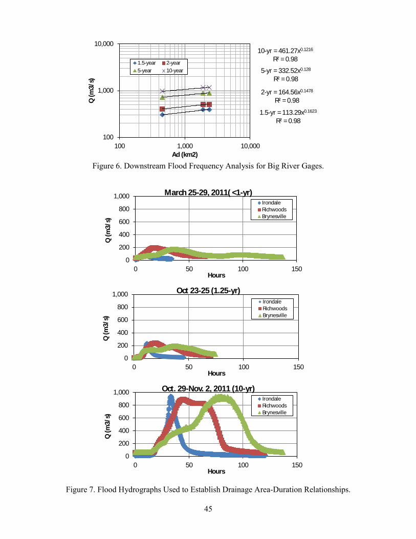
45

Figure 6. Downstream Flood Frequency Analysis for Big River Gages.

Figure 7. Flood Hydrographs Used to Establish Drainage Area-Duration Relationships.

1.5-yr = 113.29x0.1623 R² = 0.98

2-yr = 164.56x0.1478 R² = 0.98

5-yr = 332.52x0.128 R² = 0.98

10-yr = 461.27x0.1216 R² = 0.98

100

1,000

10,000

100 1,000 10,000

Q (

m3

/s)

Ad (km2)

1.5-year 2-year

5-year 10-year

0

200

400

600

800

1,000

0 50 100 150

Q (

m3

/s)

Hours

March 25-29, 2011( <1-yr) Irondale

Richwoods

Brynesville

0

200

400

600

800

1,000

0 50 100 150

Q (

m3

/s)

Hours

Oct 23-25 (1.25-yr) Irondale

Richwoods

Brynesville

0

200

400

600

800

1,000

0 50 100 150

Q (

m3

/s)

Hours

Oct. 29-Nov. 2, 2011 (10-yr) Irondale

Richwoods

Brynesville

46

Figure 8. Project Period Rainfall Compared to Historical Rainfall Records From St. Louis, Missouri.

Figure 9. Hydrograph at the Irondale Gage Located 30 km Upstream of the Bar Site With Flood Frequency.

-30

-20

-10

0

10

20

30

Rai

nfal

l (cm

)

Month

Departure from Mean Monthly Rainfall Totals for St. Louis, Missouri

Annual mean = 95 cm June 2009-May 2010 = 125 cm

Project Period

0.1

1

10

100

1000

10000

0 50 100 150 200 250

Q (

m3/s

)

Days

Q 1.1 Q 1.5 Q 2.33 Q 5 Q 10

Excavation

Post-Ex. Survey Post-Bf. Survey

Post-Fld. Survey

Flood

Bankfull Events

Post-Ex. Bankfull

47

Figure 10. Changes in Bone Hole Cross-Section at Station R-km 165.4 in the A.) Pre-Excavation Survey, B.) Post-Excavation Survey, C.) Post-Flood Survey and D.) Post-Bankfull Survey.

171

172

173

174

175

0 10 20 30 40 50

Ele

vati

on

(m

)

Distance (m)

Pre-Excavation Survey July 30, 2009

171

172

173

174

175

0 10 20 30 40 50

Ele

vati

on

(m

)

Distance (m)

Post-Excavation Survey October 20, 2009

171

172

173

174

175

0 10 20 30 40 50

Ele

vati

on

(m

)

Distance (m)

Post-Flood Survey November 5, 2009

171

172

173

174

175

0 10 20 30 40 50

Ele

vati

on

(m

)

Distance (m)

Post-Bankfull Survey March 10, 2010

Transect

Previous Transect

A.

B.

C.

D.

48

Figure 11. Absolute Volume Changes Measured at the Bone Hole Relative to Pre-Excavation Condition.

-500

-400

-300

-200

-100

0

100

200

300

400

500

Bone Hole Bone Hole Pit

Vo

lum

e (

m3 )

Sites

Post-Excavation

Post-Flood

Post-Bankfull

49

Figure 12. Changes at the Bar Head, Cross-Section at Station R-km 163.4 in the A.) Pre-Excavation Survey, B.) Post-Excavation Survey, C.) Post-Flood Survey and D.) Post-Bankfull Survey.

204

205

206

207

208

0 10 20 30 40 50El

eva

tio

n (

m)

Distance (m)

Pre-Excavation Survey July 29, 2009

204

205

206

207

208

0 10 20 30 40 50

Ele

vati

on

(m

)

Distance (m)

Post-Excavation Survey October 21, 2009

204

205

206

207

208

0 10 20 30 40 50

Ele

vati

on

(m

)

Distance (m)

Post-Flood Survey November 5, 2009

204

205

206

207

208

0 10 20 30 40 50

Ele

vati

on

(m

)

Distance (m)

Post-Bankflood Survey March 11, 2010

Transect

Previous Transect

A.

B.

C.

D.

50

Figure 13. Changes at the Bar Middle, Cross-Section at Station R-km 163.4 in the A.) Pre-Excavation Survey, B.) Post-Excavation Survey, C.) Post-Flood Survey and D.) Post-Bankfull Survey.

204

205

206

207

208

0 10 20 30 40 50 60El

eva

tio

n (

m)

Distance (m)

Pre-Excavation Survey July 29, 2009

204

205

206

207

208

0 10 20 30 40 50 60

Ele

vati

on

(m

)

Distance (m)

Post-Excavation Survey October 21, 2009

204

205

206

207

208

0 10 20 30 40 50 60

Ele

vati

on

(m

)

Distance (m)

Post-Flood Survey November 5, 2009

204

205

206

207

208

0 10 20 30 40 50 60

Ele

vati

on

(m

)

Distance (m)

Post-Bankfull Survey March 11, 2010

Transect

Previous Transect

A.

B.

C.

D.

51

Figure 14. Changes at the Bar Tail, Cross-Section at Station R-km 163.4 in the A.) Pre-Excavation Survey, B.) Post-Excavation Survey, C.) Post-Flood Survey and D.) Post-Bankfull Survey.

204

205

206

207

208

209

0 10 20 30 40 50 60

Ele

vati

on

(m

)

Distance (m)

Pre-Excavation Survey July 29, 2009

204

205

206

207

208

209

0 10 20 30 40 50 60

Ele

vati

on

(m

)

Distance (m)

Post-Excavation Survey October 21, 2009

204

205

206

207

208

209

0 10 20 30 40 50 60

Ele

vati

on

(m

)

Distance (m)

Post-Flood Survey November 5, 2009

204

205

206

207

208

209

0 10 20 30 40 50 60

Ele

vati

on

(m

)

Distance (m)

Post-Bankfull Survey March 11, 2010

Transect

A.

B.

C.

D.

52

Figure 15. Absolute Changes in Measured Volume at the Bar Site Relative to Pre-Excavation Condition.

-500

-400

-300

-200

-100

0

100

200

300

400

500

Bar Site Bar Head Bar Mid Bar Tail

Vo

lum

e (

m3 )

Sites

Post-Excavation

Post-Flood

Post-Bankfull

53

Figure 16. Average Particle Size Distribution from Samples Collected From the Bone Hole.

Figure 17. Sediment Composition of Samples Collected From the Bone Hole.

Figure 18. Average Concentration of Metals in Samples Collected From the Bone Hole.

0

10

20

30

40

50

60

<2 2-4 4-8 8-16 16-32 32-64 >64

% B

y M

ass

Particle Size (mm)

Bone Hole Particle Size Distribution

Pre-excavation

Post-excavation

Post-flood

Post-bankfull

0

10

20

30

40

50

60

70

80

Dolomite Natural Shale Quartz Slag

Ave

rage

Pe

rce

nt

of

Sam

ple

Material

Bone Hole Sediment Source ID

Pre-excavation

Post-excavation

Post-flood

0

1,000

2,000

3,000

4,000

Pre-exc Post-exc Post-flood Post-bankfull

Co

nce

ntr

atio

n (

pp

m)

Bone Hole Metal Concentrations

Lead

Zinc

54

Figure 19. Average Particle-Size Distribution From Samples Collected at the Bar Site.

Figure 20. Sediment Composition of Samples Collected at the Bar Site.

Figure 21. Average Concentration of Metals in Samples Collected From the Bar Site.

0

10

20

30

40

50

60

<2 2-4 4-8 8-16 16-32 32-64 >64

% B

y M

ass

Particle Size (mm)

Bar Particle Size Distribution

Pre-excavation

Post-excavation

Post-flood

Post-bankfull

0

10

20

30

40

50

60

70

80

Dolomite Natural Shale Quartz Slag

Ave

rage

Per

cen

t o

f Sa

mp

le

Material

Bar Sediment Source ID

Pre-excavation

Post-excavation

Post-flood

0

1,000

2,000

3,000

4,000

Pre-exc Post-exc Post-flood Post-bankfull

Co

nce

ntr

atio

n (

pp

m)

Bar Metal Concentrations

Lead

Zinc

55

Figure 22. Drainage Area-Duration Relationships the A.) Base and B.) 95% Peak from Hydrographs for Selected Floods at Big River Gages.

10-yr = 0.6865x0.6656 R² = 1

<1-yr = 0.1468x0.7649 R² = 0.98

1.25-yr = 0.1894x0.7426 R² = 0.98

10

100

1,000

100 1,000 10,000

Du

rati

on

(h

rs)

Ad (km2)

10-yr

1.25-yr

<1-yr

10-yr = 0.0009x1.2542 R² = 0.99

<1-yr = 0.0029x1.0151 R² = 0.95

1.25-yr = 0.0061x0.9428 R² = 0.94

1

10

100

100 1,000 10,000

Du

rati

on

(h

rs)

Ad (km2)

10-yr

1.25-yr

<1-yr

56

Figure 23. Channel Hydrologic Characteristics at Station R-km 163.4 Near the Bar Site Cross-Section.

Figure 24. Longitudinal Profile at the Bar Site.

Figure 25. Grain-Size Distribution at the Bar Site.

282930313233343536373839

0 50 100 150 200

Re

l. E

leva

tio

n (

m)

Distance (m)

Cross-section at Station 164.4 km

Transect

Bankfull

Terrace

High Water Mark

27.427.627.828.028.228.428.628.829.029.229.4

0 100 200 300 400

Re

lati

ve E

leva

tio

n (

m)

Distance (m)

Water SurfaceThalweg Profile

Slope = 0.001

0

20

40

60

80

100

1 10 100

Pe

rce

nt

Fin

er

Grain Size (mm)

57

Figure 26. Bedload Transport Rating Curve Evaluation A.) Rating Curve and B.) Analysis of Model Fit Comparing Both Full and Partial Datasets.

y = -8E-06x3 + 0.0135x2 - 0.5376x + 2.168 R² = 1

1

10

100

1,000

10,000

10 100 1,000

Be

dlo

ad T

ran

spo

rt R

ate

(kg

/min

)

Q (m3/s)

1

10

100

1,000

10,000

1 10 100 1,000 10,000

Pre

dic

ted

Be

dlo

ad T

ran

spo

rt (

kg/m

in)

BAGS Bedload Transport (kg/min)

Partial Dataset

Full Dataset

1:1 Line

A.

B.

58

APPENDIX A – Flood Frequency Data Irondale

Date Q (m3/s) Rank Flood Freq. (yrs)

11/14/1993 1,391 1 46

11/1/1972 1,223 2 23

11/19/1985 1,121 3 15.3

5/8/2009 1,042 4 11.5

10/30/2009 937 5 9.2

1/29/1969 782 6 7.7

8/9/1970 773 7 6.6

5/8/2002 745 8 5.8

4/11/1979 739 9 5.1

2/9/1966 731 10 4.6

3/18/2008 725 11 4.2

3/28/1977 666 12 3.8

2/23/1985 666 13 3.5

11/23/1983 640 14 3.3

4/22/1996 640 15 3.1

8/27/1982 595 16 2.9

6/25/1993 592 17 2.7

2/27/1997 510 18 2.6

12/3/1982 507 19 2.4

5/16/1990 507 20 2.3

2/22/1975 504 21 2.2

2/7/1999 445 22 2.1

4/16/1972 439 23 2.0

12/1/2006 411 24 1.9

3/12/2006 396 25 1.84

11/25/1973 394 26 1.77

3/7/1995 382 27 1.70

4/4/1968 360 28 1.64

10/13/1970 329 29 1.59

1/13/2005 323 30 1.53

3/19/1998 314 31 1.48

2/13/1989 274 32 1.44

4/14/1991 270 33 1.39

12/25/1987 266 34 1.35

4/19/1992 261 35 1.31

5/18/1981 244 36 1.28

7/10/1978 215 37 1.24

1/26/1967 207 38 1.21

7/31/1976 195 39 1.18

2/24/2001 194 40 1.15

5/1/2004 137 41 1.12

10/29/2002 134 42 1.10

10/1/1986 125 43 1.07

3/30/1980 43 44 1.05

12/10/1999 39 45 1.02

59

Richwoods Date Q (m3/s) Rank Flood Freq. (yrs)

9/23/1993 1,694 1 46

3/19/2008 1,495 2 23

4/11/1994 1,430 3 15.3

5/1/1983 1,408 4 11.5

11/19/1985 1,274 5 9.2

4/12/1979 929 6 7.7

10/30/2009 889 7 6.6

5/26/1990 864 8 5.8

3/28/1977 835 9 5.1

1/30/1969 827 10 4.6

2/23/1985 818 11 4.2

5/9/2009 736 12 3.8

11/2/1972 731 13 3.5

3/12/2006 731 14 3.3

5/9/2002 677 15 3.1

6/22/1997 637 16 2.9

4/22/2005 606 17 2.7

2/10/1966 603 18 2.6

4/29/1996 603 19 2.4

5/18/1995 600 20 2.3

4/30/1967 595 21 2.2

12/21/1967 586 22 2.1

2/23/1975 581 23 2.0

11/24/1983 581 24 1.9

2/7/1999 549 25 1.84

12/10/1971 532 26 1.77

3/20/1998 518 27 1.70

12/30/1990 515 28 1.64

1/31/1982 510 29 1.59

5/19/1981 470 30 1.53

2/22/1974 450 31 1.48

12/26/1987 439 32 1.44

12/2/2006 408 33 1.39

4/20/1992 388 34 1.35

3/25/1978 343 35 1.31

5/1/1970 340 36 1.28

5/7/2003 317 37 1.24

11/18/2003 261 38 1.21

2/14/1989 253 39 1.18

10/14/1970 197 40 1.15

10/2/1986 195 41 1.12

2/25/2001 158 42 1.10

8/16/1980 157 43 1.07

5/7/2000 155 44 1.05

12/16/1975 80 45 1.02

60

Byrnesville Date Q (cms) Rank Flood Freq. (yrs)

9/25/1993 1,801 1 46.0

11/16/1993 1,436 2 23.0

3/20/2008 1,340 3 15.3

11/21/1985 1,218 4 11.5

5/2/1983 1,212 5 9.2

4/13/1979 1,025 6 7.7

11/1/2009 943 7 6.6

5/27/1990 923 8 5.8

1/31/1969 855 9 5.1

11/4/1972 793 10 4.6

5/19/1995 787 11 4.2

2/25/1985 770 12 3.8

12/31/1990 742 13 3.5

4/29/1996 739 14 3.3

3/30/1977 719 15 3.1

5/10/2009 719 16 2.9

5/10/2002 674 17 2.7

5/7/2000 663 18 2.6

3/13/2006 603 19 2.4

2/24/1975 575 20 2.3

12/23/1967 572 21 2.2

3/21/1998 564 22 2.1

2/11/1966 538 23 2.0

6/23/1997 521 24 1.9

2/9/1999 504 25 1.84

12/12/1971 498 26 1.77

2/1/1982 484 27 1.70

12/27/1987 459 28 1.64

4/23/2005 450 29 1.59

5/21/1981 442 30 1.53

12/26/1973 436 31 1.48

11/25/1983 425 32 1.44

4/21/1992 396 33 1.39

5/7/2003 391 34 1.35

5/1/1967 385 35 1.31

3/26/1978 368 36 1.28

10/1/1986 360 37 1.24

12/3/2006 343 38 1.21

5/2/1970 317 39 1.18

11/19/2003 226 40 1.15

2/15/1989 199 41 1.12

2/26/2001 157 42 1.10

2/23/1971 151 43 1.07

3/31/1980 89 44 1.05

12/16/1975 78 45 1.02

61

APPENDIX B – Survey Maps

62

63

64

65

66

67

68

69

APPENDIX C – Volume Changes by Survey

Bone Hole

Survey Post-

Excavation** Post-Flood Q Post-Bankfull Q

Survey Date Oct. 20, 2009 Nov. 5, 2009 March 10, 2010

Reach -195 -206 -64

Pit -405 +326 -4

* + sign equals increase in channel material, - sign equals decrease in channel material **Excavated volume = 388 m3 (508 yd3) Bar Site

Survey Post-

Excavation** Post-Flood Q Post-Bankfull Q

Survey Date Oct. 20, 2009 Nov. 5, 2009 March 10, 2010

Reach -187 +339 -547

Head -172 +209 -169

Mid -96 -51 -196

Tail +81 +182 -183

* + sign equals increase in channel material, - sign equals decrease in channel material **Excavated volume = 275 m3 (360 yd3)

70

APPENDIX D – Sediment Sample Data

Bone Hole Sediment Sample Data

Sediment Source (% by Weight?) Grain-size Distribution (%) Geochemistry

Sample # Dolomite Natural Shale Quartz Slag <2 2-4 4-8 8-16 16-32 32-64 >64 Pb (ppm)

Zn (ppm)

Pre-Excavation Survey

G-49 40.4 58.6 0.0 0.0 1.0 34 11 12 17 14 13 0 2,182 6,344

G-50 35.3 56.5 0.0 2.4 5.9 29 18 17 12 14 11 0 2,200 882

Post-Excavation Survey

B-128 34 63 0 1 2 22 19 27 19 14 0 0 989 1,320

B-129 “Slime” Deposit 20,695 3,755

B-130 40 57 0 0 3 26 19 22 13 20 0 0 1,978 859

B-131 3 90 0 0 7 26 18 20 17 19 0 0 1,040 1,536

B-132 35 64 0 0 1 29 22 22 14 12 0 0 2,183 700

Post-Flood Survey

B-152 18 78 0 1 3 100 0 0 0 0 0 0 572 1,146

B-153 27 70 0 1 2 16 22 38 20 4 0 0 907 4,279

B-154 33 63 0 1 2 40 21 27 4 9 0 0 821 1,208

Post-Bankfull Survey

G-66 18 16 27 22 13 4 0 1,454 1,065

G-67 34 23 24 13 6 0 0 1,307 1,185

G-68 20 24 26 16 9 4 0 894 2,194

G-69 13 14 21 28 18 6 0 1,004 2,202

71

Bar Site Sediment Sample Data

Sediment Source (% by Weight) Grain-size Distribution (%) Geochemistry

Sample # Dolomite Natural Shale Quartz Slag <2 2-4 4-8 8-16 16-32 32-64 >64 Pb (ppm)

Zn (ppm)

Pre-Excavation Survey B-124 45 72 0 2 4 22 25 25 24 4 0 0 1,212 912

B-125 29 65 1 1 5 20 12 22 28 18 0 0 837 892

B-126 55 99 0 2 3 40 20 20 15 5 0 0 1,190 4,653

B-127 48 63 1 2 3 43 12 17 16 12 0 0 933 891

Post-Excavation Survey B-133 36 60 0 0 1 40 22 17 12 10 0 0 1,621 1,174

B-134 38 42 0 1 5 40 15 17 16 13 0 0 967 3,360

B-135 37 54 0 2 9 45 13 18 13 11 0 0 1,175 2,851

B-136 12 61 0 1 5 46 20 19 12 3 0 0 829 1,846

B-137 10 75 1 4 6 54 16 20 8 3 0 0 751 3,484

B-138 39 46 2 1 3 49 10 16 14 12 0 0 1,030 2,373

B-139 31 60 0 1 1 49 17 18 13 3 0 0 803 2,222

B-140 23 83 0 0 5 60 24 10 6 0 0 0 1,619 1,325

B-141 47 56 0 0 1 20 21 26 20 13 0 0 1,121 3,277

B-142 14 63 3 0 3 40 16 21 14 9 0 0 1,071 2,693

B-155 41 68 2 0 0 67 15 11 20 2 0 0 686 1,242

Post-Flood Survey B-143 3 73 0 0 1 16 19 30 24 12 0 0 1,053 1,002

B-144 35 68 2 0 2 35 12 16 21 16 0 0 907 966

B-145 17 59 0 1 3 45 14 19 11 11 0 0 561 1,999

B-146 62 52 0 2 2 41 12 15 11 21 0 0 721 1,156

B-147 11 60 0 1 0 26 9 13 15 37 0 0 2,913 3,310

B-148 38 56 0 1 4 33 20 29 18 0 0 0 1,243 1,395

B-149 44 66 0 2 4 34 25 22 13 6 0 0 1,022 1,041

B-150 30 70 0 1 1 62 21 16 1 0 0 0 679 1,115

Post-Bankfull Survey B-158 41 13 15 18 13 0 0 1,175 1,086

B-159 46 13 18 15 7 0 0 930 1,612

B-160 26 25 29 19 2 0 0 597 1,726

72

APPENDIX E – Sediment Sample Locations Bone Hole

Sample # Period UTM (NAD83)

Zone 15N Easting

UTM (NAD83) Zone 15N Northing

G-49 Pre-Excavation 715,442.76 4,194,793.30 G-50 Pre-Excavation 715,451.12 4,194,813.42 B-128 Post-Excavation 715,428.07 4,194,795.43 B-129 Post-Excavation 715,430.56 4,194,790.57 B-130 Post-Excavation 715,422.30 4,194,780.76 B-131 Post-Excavation 715,442.89 4,194,801.92 B-132 Post-Excavation 715,441.86 4,194,811.32 B-152 Post-Flood 715,436.51 4,194,782.47 B-153 Post-Flood 715,434.43 4,194,797.93 B-154 Post-Flood 715,453.07 4,194,814.62 G-66 Post-Bankfull 715,431.20 4,194,783.07 G-67 Post-Bankfull 715,433.82 4,194,791.85 G-68 Post-Bankfull 715,428.44 4,194,799.26 G-69 Post-Bankfull 715,426.96 4,194,807.83

Bar Site

Sample # Period UTM (NAD83)

Zone 15N Easting

UTM (NAD83) Zone 15N Northing

B-124 Pre-Excavation 714,573.03 4,196,244.74 B-125 Pre-Excavation 714,561.22 4,196,237.32 B-126 Pre-Excavation 714,554.22 4,196,300.72 B-127 Pre-Excavation 714,530.70 4,196,279.35 B-133 Post-Excavation 714,587.55 4,196,219.09 B-134 Post-Excavation 714,571.66 4,196,233.37 B-135 Post-Excavation 714,568.02 4,196,249.06 B-136 Post-Excavation 714,552.19 4,196,240.11 B-137 Post-Excavation 714,545.14 4,196,239.28 B-138 Post-Excavation 714,552.59 4,196,262.83 B-139 Post-Excavation 714,540.12 4,196,257.69 B-140 Post-Excavation 714,533.57 4,196,251.28 B-141 Post-Excavation 714,548.16 4,196,284.59 B-142 Post-Excavation 714,529.94 4,196,278.85 B-155 Post-Excavation 714,553.73 4,196,327.36 B-143 Post-Flood 714,566.23 4,196,275.46 B-144 Post-Flood 714,555.91 4,196,269.82 B-145 Post-Flood 714,540.12 4,196,259.71 B-146 Post-Flood 714,547.09 4,196,252.95 B-147 Post-Flood 714,565.81 4,196,256.20 B-148 Post-Flood 714,554.91 4,196,293.72 B-149 Post-Flood 714,555.55 4,196,323.33 B-150 Post-Flood 714,554.81 4,196,328.64 B-158 Post-Bankfull 714,569.86 4,196,241.99 B-159 Post-Bankfull 714,537.44 4,196,263.48 B-160 Post-Bankfull 714,551.32 4,196,314.08

73

APPENDIX F – Pebble Count Data

GLIDE RIFFLE

GLIDE RIFFLE GRID GRID HEAD TAIL

GRID GRID HEAD TAIL

n=30 n=30 n=30 n=30

n=30 n=30 n=30 n=30

16 5.6 32 2.8

5.6 2.8 32 5.6 0.1 8 8 2.8

11 5.6 45 4

11 11 16 5.6

11 4 16 8 22.6 16 11 5.6

4 22.6 11 16

16 8 45 8

11 5.6 22.6 5.6 11 11 16 5.6

2 5.6 22.6 5.6

16 8 32 2.8

5.6 16 11 22.6 16 11 5.6 11

4 16 22.6 5.6

5.6 16 22.6 2.8

16 11 16 5.6 0.1 5.6 8 2.8

2 5.6 11 4

2.8 8 22.6 11

2 5.6 32 2 16 2.8 5.6 2.8

2 5.6 32 4

16 8 16 5.6

8 8 16 2 16 11 11 11

4 8 16 2

2.8 11 22.6 2.8

2 5.6 22.6 5.6 16 11 11 5.8

2 8 11 4

11 5.6 11 8

8 16 32 5.6 8 5.6 22.6 8

2 11 32 16

22.6 5.6 32 2.8

2 16 32 5.6 8 11 5.6 16

5.6 32 32 8

11 8 16 5.6

2.8 5.6 22.6 8 22.6 5.6 16 2.8

4 5.6 32 4

16 11 16 2.8

8 32 5.6 5.6 22.6 22.6 22.6 8

11 32 32 8

11 11 22.6 4

2.8 22.6 32 4 0.1 32 32 5.6

5.6 16 45 16

2.8 11 11 32

4 11 11 2 22.6 5.6 22.6 22.6

2.8 22.6 16 8

11 8 8 4

4 22.6 5.6 2.8 8 11 22.6 8

4 16 5.6 2

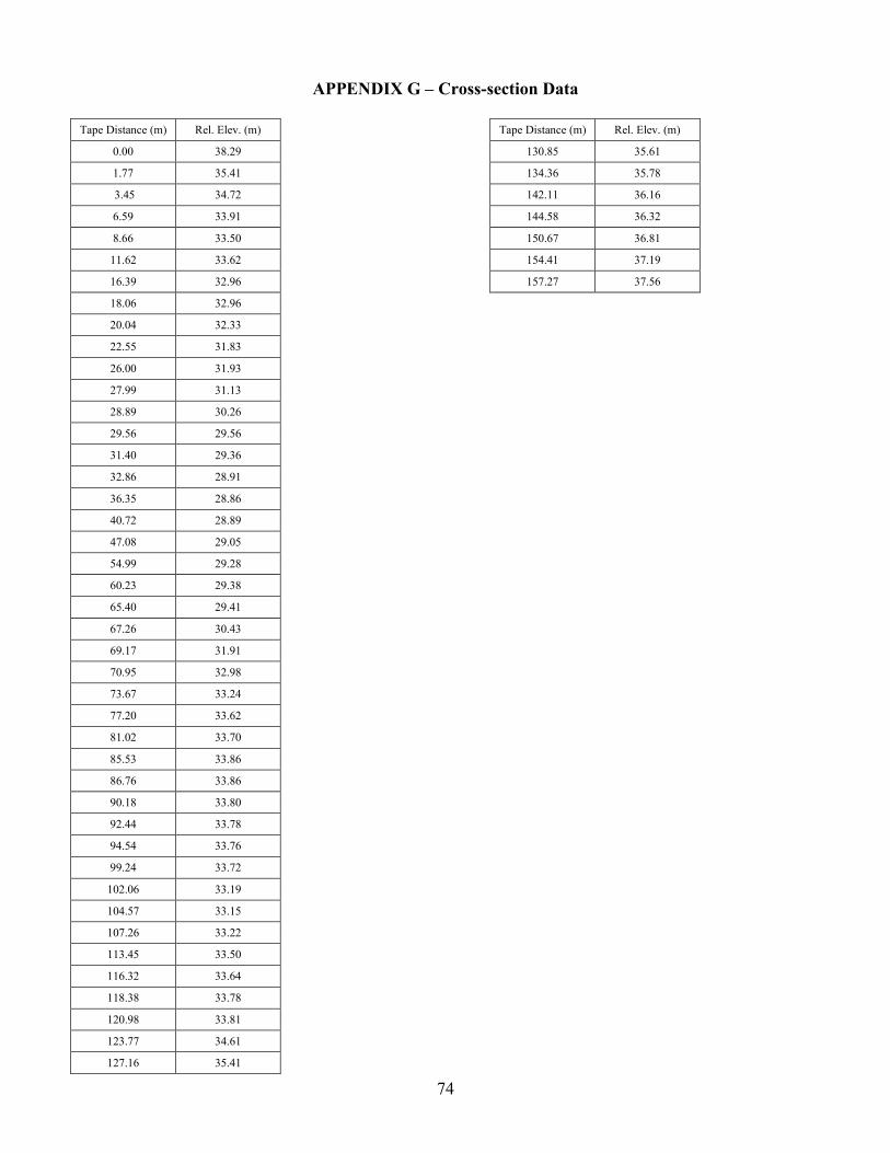
74

APPENDIX G – Cross-section Data

Tape Distance (m) Rel. Elev. (m) Tape Distance (m) Rel. Elev. (m)

0.00 38.29 130.85 35.61

1.77 35.41 134.36 35.78

3.45 34.72 142.11 36.16

6.59 33.91 144.58 36.32

8.66 33.50 150.67 36.81

11.62 33.62 154.41 37.19

16.39 32.96 157.27 37.56

18.06 32.96

20.04 32.33

22.55 31.83

26.00 31.93

27.99 31.13

28.89 30.26

29.56 29.56

31.40 29.36

32.86 28.91

36.35 28.86

40.72 28.89

47.08 29.05

54.99 29.28

60.23 29.38

65.40 29.41

67.26 30.43

69.17 31.91

70.95 32.98

73.67 33.24

77.20 33.62

81.02 33.70

85.53 33.86

86.76 33.86

90.18 33.80

92.44 33.78

94.54 33.76

99.24 33.72

102.06 33.19

104.57 33.15

107.26 33.22

113.45 33.50

116.32 33.64

118.38 33.78

120.98 33.81

123.77 34.61

127.16 35.41

75

APPENDIX H – BAGS Model Output

Discharge (m3/s)

Bedload transport

rate (kg/min)

Transport Stage (m)

Max water depth (m)

Hydraulic radius (m)

Sediment transport rate by size, in kg/min. Sediment transport by size, (% of total)

1 - 2 mm

2 – 4 mm

4 - 8 mm

8 - 16 mm

16 - 32 mm

32 - 64 mm

1 - 2 mm

2 – 4 mm

4 - 8 mm

8 - 16 mm

16 - 32 mm

32 - 64 mm

40.0 3.46 1.32 1.50 1.15 0.78 1.14 1.25 0.28 0.01 0.00 22.7 32.9 36.3 8.0 0.2 0.0

45.7 6.00 1.43 1.60 1.23 1.26 1.91 2.28 0.55 0.01 0.00 21.0 31.8 37.9 9.1 0.2 0.0

52.1 10.02 1.54 1.71 1.33 1.95 3.07 3.90 1.08 0.02 0.00 19.4 30.7 38.9 10.8 0.2 0.0

59.5 16.20 1.66 1.82 1.43 2.93 4.77 6.38 2.07 0.04 0.00 18.1 29.5 39.4 12.8 0.3 0.0

68.0 25.04 1.78 1.95 1.54 4.25 7.11 9.93 3.66 0.08 0.00 17.0 28.4 39.7 14.6 0.3 0.0

77.6 37.27 1.91 2.09 1.66 5.99 10.26 14.83 6.03 0.16 0.00 16.1 27.5 39.8 16.2 0.4 0.0

88.6 55.12 2.06 2.24 1.79 8.41 14.70 21.94 9.75 0.31 0.00 15.3 26.7 39.8 17.7 0.6 0.0

101.2 78.17 2.21 2.40 1.91 11.42 20.30 31.06 14.80 0.59 0.00 14.6 26.0 39.7 18.9 0.8 0.0

115.5 109.2 2.37 2.58 2.05 15.32 27.64 43.25 21.88 1.13 0.00 14.0 25.3 39.6 20.0 1.0 0.0

131.9 149.7 2.53 2.77 2.19 20.22 36.97 58.98 31.40 2.11 0.00 13.5 24.7 39.4 21.0 1.4 0.0

150.6 201.8 2.71 2.98 2.34 26.35 48.71 79.06 43.98 3.70 0.00 13.1 24.1 39.2 21.8 1.8 0.0

171.9 265.3 2.87 3.21 2.49 33.64 62.79 103.3 59.59 5.96 0.00 12.7 23.7 38.9 22.5 2.2 0.0

196.3 356.1 3.09 3.43 2.68 43.65 82.34 137.6 82.54 9.91 0.00 12.3 23.1 38.7 23.2 2.8 0.0

224.1 471.9 3.33 3.67 2.88 56.06 106.8 181.0 112.3 15.74 0.00 11.9 22.6 38.3 23.8 3.3 0.0

255.9 618.0 3.58 3.93 3.10 71.33 137.0 235.1 150.5 24.07 0.01 11.5 22.2 38.0 24.4 3.9 0.0

292.2 792.9 3.82 4.22 3.31 89.26 172.7 299.4 196.6 34.90 0.02 11.3 21.8 37.8 24.8 4.4 0.0

333.6 1,020 4.11 4.52 3.56 111.9 218.1 382.1 257.4 50.59 0.03 11.0 21.4 37.5 25.2 5.0 0.0

380.9 1,311 4.44 4.81 3.84 140.2 275.1 486.9 336.2 72.75 0.06 10.7 21.0 37.1 25.6 5.5 0.0

434.9 1,659 4.78 5.13 4.14 173.3 342.1 611.2 431.2 101.3 0.11 10.4 20.6 36.8 26.0 6.1 0.0

496.5 2,067 5.14 5.45 4.45 211.3 419.6 755.6 543.4 137.1 0.19 10.2 20.3 36.6 26.3 6.6 0.0

566.9 2,553 5.52 5.79 4.78 255.8 510.6 926.1 677.6 182.1 0.31 10.0 20.0 36.3 26.5 7.1 0.0

647.3 3,128 5.93 6.16 5.13 307.7 617.1 1,127 837.6 238.3 0.49 9.8 19.7 36.0 26.8 7.6 0.0

739.0 3,811 6.36 6.55 5.51 368.4 742.1 1,364 1,028 308.0 0.73 9.7 19.5 35.8 27.0 8.1 0.0

843.8 4,632 6.83 6.97 5.91 440.3 890.6 1,646 1,258 395.3 1.07 9.5 19.2 35.5 27.2 8.5 0.0

963.4 5,597 7.33 7.42 6.34 523.8 1,064 1,976 1,530 502.0 1.53 9.4 19.0 35.3 27.3 9.0 0.0

1,100 6,713 7.85 7.89 6.80 619.1 1,261 2,356 1,845 629.5 2.12 9.2 18.8 35.1 27.5 9.4 0.0

76

APPENDIX I –Site Photographs

Low-water bridge at Bone Hole

Looking downstream toward low-water bridge

77

Pre-excavation survey at Bone Hole, looking downstream toward low-water bridge.

Looking upstream at Bone Hole. Owl Creek tributary enters from left.

78

Excavation activities at the Bone Hole site are consistent with post-excavation survey results. (Photos from HGL Field Oversight Report).

Looking up the Site #2 bar from the tail

79

Looking downstream from the tail end of Site #2 Bar

Surveying at Site #2 Bar. Notice survey tape and orange flags marking the 10m increment cross-section

80

Looking upstream across excavated bar head. Notice excavator tracks and flat topography.

Looking downstream at recently excavated bar head.

81

Looking upstream at bar tail.

Looking downstream at bar head, post-flood.

82

Looking downstream across bar, post-flood.