bid shading and bidder surplus in the u.s. treasury ... · bid shading and bidder surplus in the...
TRANSCRIPT

Bid Shading and Bidder Surplus in the U.S. Treasury Auction
System ∗
Ali Hortacsu† Jakub Kastl‡ Allen Zhang§
November 13, 2014
(PRELIMINARY AND INCOMPLETE: PLEASE DO NOT CITE OR DISTRIBUTE
WITHOUT PERMISSION.) We analyze detailed bidding data from auctions of Treasury bills
and notes conducted between July 2009 and October 2013. The U.S. Treasury uses a uniform
price auction system, which we model building on the share auction model of Wilson (1979) and
Kastl (2012). Our model takes into account informational asymmetries introduced by the primary
dealership and indirect bidding system employed by the U.S. Treasury. Building on the methods de-
veloped by Hortacsu (2002), Hortacsu and McAdams (2010), Kastl (2011), and Hortacsu and Kastl
(2012), we estimate the amount of bid shading undertaken by the bidders under the assumption of
bidder optimization. Our method also enables to us to estimate the marginal valuations of bidders
that rationalize the observed bids under a private value framework. We find that primary dealers
consistently bid higher yields in the auctions compared to direct and indirect bidders. Our model
allows us to decompose this difference into two components: difference in demand/willingness-to-
pay, and difference in ability to shade bids. We find that while primary dealer willingness-to-pay
is similar to or even higher than direct and indirect bidders’, their ability to bid-shade is higher,
leading to higher yield bids. By computing the area under bidders’ demand curves, we can also
quantify the surplus that bidders derive from the auctions. We find that total bidder surplus across
the sample period was, on average, 2.3 basis points.
Keywords: multiunit auctions, treasury auctions, structural estimation, nonparametric identification
and estimation JEL Classification: D44
∗The views expressed in this paper are those of the authors and should not be interpreted as reflecting the viewsof the U.S. Department of the Treasury. Kastl is grateful for the financial support of the NSF (SES-1352305) andthe Sloan Foundation, Hortacsu the financial support of the NSF (SES-1124073). All remaining errors are ours.†Department of Economics, University of Chicago, and NBER‡Department of Economics, Princeton University, and NBER§U.S. Department of Treasury
1
1 Introduction
In 2013, the U.S. Treasury auctioned 7.9 trillion dollars of government debt (TreasuryDirect.gov) to
a global set of institutions and investors. The debt was issued in a variety of instruments, covering
bills (up to 1 year maturity), 2-10 year notes, 30 year coupon bonds, and Treasury Inflation-
Protected Securities (TIPS). The mandate of the U.S. Treasury is to achieve the lowest cost of
financing over time, taking into account considerable uncertainty in the borrowing needs of the
government and demand for U.S. Treasuries by investors.1 Treasury also seeks to ”facilitate regular
and predictable issuance” across a range of maturity classes. To this end, the Treasury adopted
auctions as their preferred method of marketing short term securities in 1920 (Garbade 2008),
and auctions became the preferred method of selling long-term securities in the 1970s (Garbade
2004). The Treasury employed a discriminatory/pay-as-bid format until 1998, when, after some
experimentation with its 2- and 5-year note auctions in 1992, the uniform price format was adopted
as the method of sale (Malvey and Archibald 1998).
This paper models the strategic behavior of auction participants, and offers model-based quan-
titative benchmarks for assessing the competitiveness and cost-effectiveness of this important mar-
ketplace. Our model builds on the seminal “share auction” model of Wilson (1979) in which bidders
are allowed to submit demand schedules as their bids. While this captures the strategic complexity
of the Treasury’s uniform price auction mechanism very well, it is in many ways related to classic
models of imperfect competition such as Cournot. In particular, consider a setting (depicted in
Figure 1) where an oligopsonistic bidder with downward sloping demand for the security knows
the residual supply function that she is facing, and is allowed to submit a single price-quantity
point as her bid. Following basic monopsony theory, this bidder will not select the competitive
outcome (P comp, Qcomp), which is the intersection of her demand curve and the residual supply
curve. Instead, she has the incentive to “shade” her bid, and pick a lower price-quantity point on
the residual supply curve, such as (P ∗, Q∗), that gives her higher surplus (the gray shaded area
below her demand curve up to (P ∗, Q∗)) than if she had bid the competitive price and quantity. Of
1Peter Fisher, then Under Secretary of Treasury for Domestic Finance, in a speech titled “Remarks before the BondMarket Association Legal and Compliance Conference” on January 8, 2002, stated that ”the overarching objectivefor the management of the Treasury’s marketable debt is to achieve the lowest borrowing cost, over time, for thefederal government’s financing needs”.
2

course, the ability of this bidder to “shade” her bid depends on the elasticity of the residual supply
curve she is facing. If this were a small bidder among many others, the residual supply she would
be facing would essentially be flat, allowing for very little ability to bid-shade, as decreasing the
quantity demanded would not result in any appreciable change in the market clearing price. The
optimal bid then is to bid one’s true demand curve.
!"
#"
$%&'()*+",)--+."
/%0*1("
2!34#35"
2!670-4#670-5"
/%0*1("
Figure 1: Illustration of Bid Shading when Residual Supply is Known
The Wilson (1979) model, and its generalization that we discuss here enhances this picture by
allowing bidders to have private information about their true demands/valuations for the securities
and to submit more than one price-quantity pair as their bids. This induces uncertainty in com-
peting bids, and thus an uncertain residual supply curve. What Wilson derives is a set (a locus)
3

of price-quantity points comprising a “bid function” that maximizes the bidder’s expected surplus
against possible realizations of the residual supply curve.
An important assumption of the Wilson setup is that bidders are allowed to bid continuous
bid functions. However, in most real world settings, bidders are confined to a discrete strategy
space that limits the number of price-quantity points they can bid. Indeed, in the auctions that we
study, bidders utilize, on average, 3 to 5 price-quantity points, with a nontrivial fraction of bidders
submitting a single step, making “discreteness” a particularly important problem. To deal with
this issue, we adopt the generalization of the Wilson model by Kastl (2011).
Yet another complication we face in this setting is the fact that bidders have inherently asym-
metric information sets. In particular, primary dealers in this market route the bids of some of
the other bidders (“indirect bidders”), and are this privy to observing a part of the residual supply
curve that other bidders do not. Our model also incorporates the reduced uncertainty/more precise
information that primary dealers possess regarding residual supply.
We develop the model to the point where we can characterize bidders’ optimal decisions in terms
of their (unobserved) “true” demands/marginal valuations, and their beliefs about the distribution
and shape of residual supply. Indeed, the optimality condition closely resembles the inverse elas-
ticity markup rule of classical monopoly theory. The optimality condition thus allows us to infer
the unobserved demands/marginal valuations of the bidders, provided that we make certain as-
sumptions regarding bidders’ beliefs. We follow, as in some of our previous work (Hortacsu (2002),
Hortacsu and McAdams (2010), Kastl (2011), and Hortacsu and Kastl (2012)) the seminal insight
of Guerre, Perrigne and Vuong (2000)2 that under the assumption that bidders have rational expec-
tations regarding the distribution and shape of residual supply, as they would if they were playing
the Bayesian-Nash equilibrium of the game, one can use the realized distribution of residual sup-
plies as an empirical estimate of bidders’ ex-ante beliefs. Once we have the bidders’ beliefs, we
can “invert” the optimality condition to recover bidders’ unobserved demand/marginal valuations
rationalizing their observed behavior.
We then utilize our estimates of bidders’ “behavior-rationalizing” marginal valuations/demand
curves to answer two sets of questions. The first is to quantify the extent of market power exercised
2and also of Elyakime, Laffont, Loisel and Vuong (1997), Laffont and Vuong (1996)
4
by bidders through bid-shading, as in Figure 1, and how this varies across different subclasses of
bidders. We find that primary dealers shade their bids more than direct and indirect bidders –
which goes towards explaining the observed differences in their bidding patterns (primary dealers
bid significantly lower prices/higher yields than direct and indirect bidders).
The second question we answer is regarding bidder surplus. In Figure 1, one can quantify the
bidder surplus by looking at the area under the bidder’s true demand curve above P ∗ and up to
Q∗. Since we have estimates of bidders’ “behavior rationalizing” demand curves, we can calculate
this area for each bidder in our data. Our main finding here is that primary dealers, perhaps not
surprisingly, extract more surplus from the auctions than direct or indirect bidders. The magnitude
of the surpluses vary quite a bit between maturity classes, with very little bidder surplus in Treasury
bills, and larger surpluses for Treasury notes.
Our surplus calculations also allow us to connect to a long literature studying the “optimal
auction mechanism” to use to sell Treasury securities. This literature dates at least back Friedman
(1960), who pointed out the bid-shading incentives of bidders in the then-used discriminatory/pay-
as-bid auction utilized by the Treasury, and advocated the use of the uniform-price auction, as
it would alleviate the bid-shading incentive of smaller bidders (for whom bidding one’s valuation
is approximately optimal) and lower their cost of participating in these auctions. However, as
noted by several authors including Wilson (1979) and Ausubel and Cramton (2002), a bid-shading
incentive remains for larger in the uniform price auction. Ausubel and Cramton (2002) also show
that optimal bid shading in these auctions also distorts the efficiency of the allocations, and thus
a general ranking of expected revenues from discriminatory and uniform price auctions can not be
made without knowledge about the specific features of bidder demand.
Given the theoretical vacuum, a variety of empirical approaches have been employed to as-
sess the efficacy of Treasury auction mechanisms. The Treasury’s own study of this question, as
reported by Malvey and Archibald (1998), was based on experimentation with the uniform price
format for 2- and 5-year notes. To assess the revenue properties of the uniform vs. the status-quo
discriminatory format, Malvey and Archibald calculated the auction-when-issued rate spread, and
did not statistically reject a mean difference across the different auction formats. However, they
5

note that the uniform price auctions “produce a broader distribution of auction awards” across
bidders, and especially a lowered concentration of awards to top primary dealers.
Our empirical approach differs from that of Malvey and Archibald’s and related studies, in that
we do not look at when-issued or secondary market prices to assess the “value” of the securities being
sold.3 Indeed, what we are interested is the “inframarginal surplus” of the bidders, which, in the
presence of downward sloping demand, will not be apparent from looking at market clearing prices
either in the primary or secondary markets. Heterogeneity in valuations that lead to downward
sloping demand for these securities may arise from many different sources: buy-and-hold bidders
may have idiosyncratic portfolio immunization needs, financial intermediaries may attach different
valuations to the Treasuries due to e.g. their use as collateral, primary dealers may value having
an inventory of Treasury beyond its resale value because being a primary creates additional value
streams (such as complementary services or access to Fed facilities).
Recovering the marginal valuations, and thus the surpluses of the bidders allows one to construct
an upper-bound to the amount of extra revenue that can be derived from switching the auction
mechanism – as no voluntary participation mechanism can extract more than the entire surplus
that would be obtained in an efficient, surplus-maximizing allocation. We find that total bidder
surplus in these auctions amounts to about 3 basis points for the average auction (though surpluses
are appreciably higher for Notes auctions than they are for Bills auctions). Assuming that the
allocations in our sample of auctions were approximately efficient, this suggests that the most cost-
savings one can hope for from a redesign of the auction mechanism will be 3 basis points. Of course,
any incentive compatible and individually rational mechanism needs to allow some surplus for the
bidders; thus, this is an extremely conservative upper bound.
The paper proceeds in the following manner. In Section 2, we describe our data, which covers
auctions conducted between July 2009 and October 2013, and the main characteristics of the U.S.
Treasury auction system. We then provide brief summary descriptions of allocation and bidding
patterns in the data by different subclasses of bidders. Section 3 develops our model of bidding that
incorporates the salient features of the U.S. Treasury auction system, and discusses the optimality
3When we looked at the differential between auction-close when-issued rates and the auction stop-out rate, wefound that our sample of auctions were “through,” i.e. the when-issued yield was systematically higher than thestop-out yield.
6

conditions that underlie our empirical strategy. Section 5 presents the results regarding bid shading
and bidder surplus.
2 Description of our Data Sample and Institutional Background
The data sample used in this study comprises of 975 auctions of Treasury securities conducted
between July 2009 and October 2013 (Table 1). The securities in our sample range from 4 week
bills to 10 year notes, with 822 auctions of 4-week, 13-week, 26-week, 52-week bills and cash
management bills, and 153 auctions of 2-year, 5-year, and 10-year notes. The total volume of
issuance through these auctions was 27.3 trillion US dollars, with the average issue size around 28
billion dollars.
The issuance mechanism is a sealed-bid uniform-price auction, which has been the preferred
auction mechanism of the Treasury since October 1998. Bids consist of price-quantity schedules and
define step functions, with minimum price increments of 0.5 basis points for thirteen, twenty-six,
fifty-two week, and cash management bills and 0.1 basis points for all other securities. Noncompet-
itive, price-taking bids are also accepted but are limited to $5 million and are usually due before
noon, an hour earlier than competitive bids. Noncompetitive bid totals are announced prior to the
deadline for competitive tenders.
Bidders in our data are categorized into three major groups: primary dealers, direct bidders, and
indirect bidders. During the sample period, 17 to 21 primary dealers regularly bid in the auctions
and made markets in Treasury securities. These primary dealers can bid on their own behalf
(“house bids”) and also submit bids on behalf of the indirect bidders.Primary dealers are, as a class
of bidders, the largest purchasers of primary issuances. In terms of tendered quantities, primary
dealer tenders comprise 69% to 88% of overall tendered quantities. Direct bidders tender 6% to 13%
and Indirect bidders 6% to 18% of the tenders.4 In terms of winning bids, or allocated quantities,
4Earlier analyses of similar tender and allocation shares by bidder classes have been performed by Garbade andIngber (2005), Fleming (2007), Fleming and Rosenberg (2007). There have been large changes in the types of biddersparticipating in and winning securities auctions since 2008, especially for longer maturity securities. In auctions fornotes and bonds, Treasury data shows there have been large increases in the proportion of both bids tendered andbids accepted by non-primary dealers. While the typical proportion of indirect bids tendered has remained relativelyconstant over the time period, Direct Bids tendered by non-primary dealers have increased from virtually none in2008 to the observed proportions in our data. This has corresponded to a decrease in the proportion of notes and
7

we find that Primary Dealers tend to win a smaller proportion of their tendered quantities. Primary
Dealers are allocated between 46% to 76% of competitive demand, while Indirect Bidders win a
disproportionate 17% to 38% (with Direct Bidders’ allocation shares staying close to their tendered
quantity shares). Let us now analyze these bidding differences more closely.
2.1 Analysis of Bid Yields and Bid Quantities
The fact that Primary Dealers are winning a smaller share of their tenders than Direct and Indirect
Bidders suggests that Primary Dealers bid systematically higher (lower) yields (prices) in these
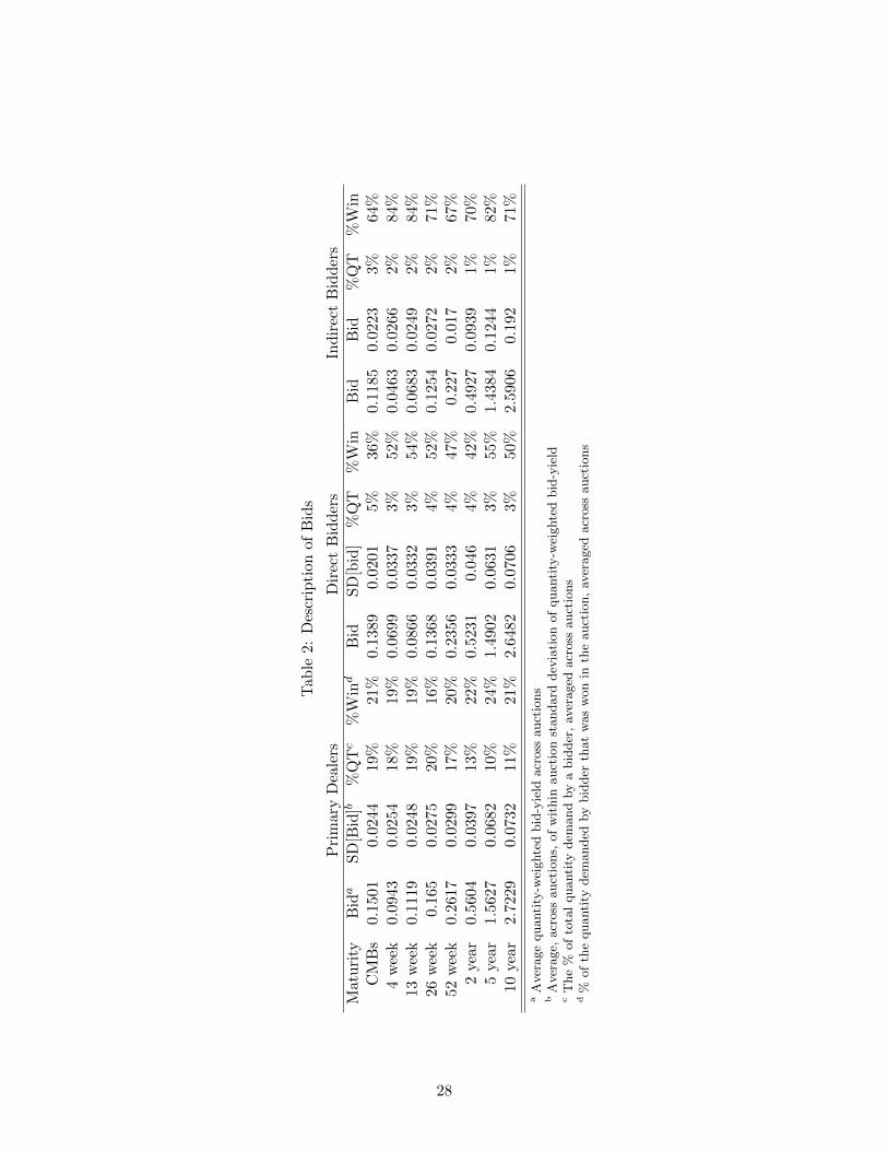
auctions. To investigate this further, Table 2 reports the quantity-weighted bid-yields submitted
by the three bidder groups across different maturities. We include the within auction standard
deviation of quantity-weighted bid yields as a measure of bid dispersion within bidder group. Since
bids in these auctions are effectively in the form of demand curves, we also include the total tender
quantity submitted by a bidder as a percentage of the issue size (%QT), and the percentage of her
tender quantity that the bidder won (%Win).
Looking at the (quantity-weighted) bid yields we see the clear pattern, across all maturities,
that Primary Dealers systematically place higher bid yields than Direct and Indirect Bidders. The
gap in bid yields between Primary Dealers and Indirect Bidders is quite substantial, and ranges
between 3 to 13 basis points depending on maturity. Primary Dealers also appear to be bidding 2
to 8 basis points higher yields than Direct Bidders.
The within-auction dispersion of (quantity-weighted) bid-yields across Primary Dealers is very
similar to the dispersion of Direct Bidder bids, ranging from 2 to 6 basis points. Indirect Bidders
submit more dispersed bids, especially for the longer-term securities, with the dispersion rising to
19 basis points for 10 year bond auctions.
Primary dealers bid for much larger quantities. The average Primary Dealer offers to purchase
between 10% to 20% of issuance, while Direct bidder quantity tenders hover between 3-5% and
Indirect Bidders’ tenders between 1-3% of the issuance. Given that Primary Dealers tend to bid
higher yields, however, it is not surprising that Primary Dealers get allocated a smaller share of
their total tenders than Direct or Indirect Bidders. Indeed, while Primary Dealers end up winning
bonds tendered by Primary Dealers.
8

only about 20% of their tendered quantities, Direct Bidders win 40-50% and Indirect Bidders,
70-80%.
2.2 Drivers of Bid Differentials?
What might drive these bid differentials across bidder groups? These different bidder groups
have different demand/willingness-to-pay for these securities, depending on their idiosyncratic
needs. Some of these bidders are buy-and-hold investors who are replenishing their bond port-
folios, while others are broker-dealers whose primary purpose is resale. In particular, it is possible
that the reason why Primary Dealers bid lower (higher yields) is that they systematically have
lower demand/willingness-to-pay for the securities than other bidder classes.
Another possibility is the exercise of market power. Even if bidders’ willingness-to-pay is the
same for the securities, the Primary Dealers, as we see, are much larger players in this market,
commanding significant market share. Such buyers may be able to exercise their monopsony power
to try to lower the marginal cost of acquisition.
Table 3 investigates the differentials in bid yields implied by Table 2 through regressions. We
have split the sample into auctions of Treasury Bills and Treasury Notes, as it is possible that the
market dynamics are very different across these different classes of securities. We also control for
auction fixed effects in each regression; thus the regressions provide within-auction comparisons
that account for differing supply-demand conditions that affect the level of the bids.
The first and third specifications regress (quantity-weighted) bid yield on indicators for Direct
and Indirect Bidders in the Bills and Notes sectors. We find here the pattern implied by Table 2:
Primary Dealers systematically (and statistically significantly) bid higher yields than Direct and
Indirect Bidders. Primary Dealer bids are 2 (4) basis points higher than Direct (Indirect) bids in
the Bills sector, and 6 (11) basis points higher in the Notes sector.
The second and fourth columns of Table 3 include the bidder’s share of the total tender size as
a proxy for bidder size. There are two main ways through which bidder size may affect the bids:
bidders demanding larger quantity may have higher demand for the security, but they may also
have higher market power. The regressions indicate that larger bidders systematically bid higher
9
yields. The effect is quite large – the coefficient estimate indicates that a size increase of 10% of
total issue size accounts for 1(6) basis point increase in the bid yield.
Accounting for bidder size appears to lower the differences in bid yields across bidder classes,
but Primary Dealers appear to bid higher yields than Direct and Indirects even accounting for their
offer share of the total issue.
As we noted above, since bids reflect both differences in demand and also differences in market
power, it is difficult to interpret these documented differences in bids. Even though we find that
larger bidders bid higher yields, this is not prima facie evidence that large bidders exercise market
power; it is possible that larger bidders also have lower demand.
In the next section, we will describe a model of bidding that will allow us to separate out the
market power and demand components of bid heterogeneity. The model, and the measurement it
will allow us to conduct, will strongly rely on the assumption of bidder optimization. In essence,
what we will end up doing is to measure the elasticity of (expected) residual supply faced by each
bidder. This is directly observable in the data, and does not require behavioral assumptions. This
elasticity will be our measure of the “potential market power” possessed by each bidder. Assuming
that bidders are expected profit maximizers who will exercise their market power in a unilateral,
noncooperative fashion, we can then estimate the willingness-to-pay/demand that rationalizes the
observed bid.
3 Model of Bidding
Our analysis is based on the share auction model of Wilson (1979) with private information, in
which both quantity and price are assumed to be continuous. Wilson’s model was modified to
take into account the discreteness of bidding (i.e., finitely many steps in bid functions) as in Kastl
(2011). In Hortacsu and Kastl (2012), we further adapted this model to allow primary dealers to
observe the bids of others, hence allowing for “indirect bidders,” whose bids are routed by primary
dealers.
Formally, suppose there are three classes of bidders: NP primary dealers (in index set P), NI
potential indirect bidders (in index set I) and ND potential direct bidders (in index set D). They
10
are each bidding for a perfectly divisible good of (random) Q units. We assume that the number
of potential bidders of each type participating in an auction, NP , NI , ND, is commonly known.
However, except primary dealers, the exact number of indirect and direct bidders is not known.
Before the bidding commences, bidders observe private (possibly multidimensional) signals.
Let us denote these signals for the different bidder groups as SP1 , ..., SPNP, Si1, ..., S
INI, SD1 , ..., S
DND
.
The bidding then proceeds in two stages. In stage 1, indirect bidders submit their bids to their
primary dealer.5 These bids, denoted by yI(p|SIj
), specify for each price p, how big a share of the
securities offered in the auction indirect bidder j demands as a function of her private information
SIj . In stage 2, direct bidders submit their bids, yD(p|SDj
), and primary dealer k submits her
customers’ bids, and also places her own bid, yP(p|SPk , ZPk
), where ZPk contains all information
dealer k observes from seeing the bids of its customers.
We will impose the following additional assumptions:
Assumption 1 Direct and indirect bidders’ and dealers’ private signals are independent and drawn
from a common support [0, 1]M according to atomless distribution functions FP (.), F I(.), and FD(.)
with strictly positive densities.
Strictly speaking, independence is not necessary for our characterization of equilibrium behavior
in this auction, but we impose it in our empirical application.
Winning q units of the security is valued according to a marginal valuation function vi (q, Si).
We assume that the marginal valuation function is symmetric within each class of bidders, but
allow it to be different across bidder classes. We will impose the following assumptions on the
marginal valuation function vg (·, ·, ·) for g ∈ {P, I,D}:
Assumption 2 vg (q, Sgi ) is non-negative, measurable, bounded, strictly increasing in (each com-
ponent of) Sgi ∀q and weakly decreasing in q ∀sgi , for g ∈ {P, I,D}.
Note that this assumption implies that learning other bidders’ signals does not affect one’s own
valuation – i.e. we have a setting with private, not interdependent values. This assumption may
be more palatable for certain securities (such as shorter term securities, which are essentially cash
5In our data, the average primary dealer routes 1.14 indirect bids, though in longer maturity auctions, primarydealers route bids from 2 to 3 indirect bidders on average.
11
substitutes) than others, but is the most tractable one under which we can pursue the “demand
heterogeneity” vs. “market power” decomposition. Note that under this assumption, the additional
information that a primary dealer j possesses due to observing her customers’ orders, ZPj , simply
consists of those submitted orders. As will become clear below, this extra piece of information allows
the primary dealer to update her beliefs about the competitiveness of the auction, or, somewhat
more precisely, the distribution of the market clearing price.
To ease notation, let θj denote private information of bidder j, i.e., for a direct bidder θj ≡ SDj ,
indirect bidder θj ≡ SIj and for a primary dealer θj ≡(SPj , Z
Pj
).
Bidders’ pure strategies are mappings from private information in each stage to bid functions
σi : Θi → Y, where the set Y includes all admissible bid functions. The expected utility of type
θi-bidder (from group g ∈ {P,D, I}) who employs a strategy ygi (·|θi) in a uniform price auction
given that other bidders are using{y
(g,−g)j (·|·)
}j 6=i
can be written as:
EUgi (θi) = EQ,Θ−i|θiug (θi,Θ−i)
= EQ,Θ−i|θi
[∫ Qci(Q,Θ,y(g,−g)(·|Θ))
0vgi (u, θi) du− P c
(Q,Θ,y(g,−g) (·|Θ)
)Qci
(Q,Θ,y(g,−g) (·|Θ)
)]
where Qci(Q,Θ,y(g,−g) (·|Θ)
)is the (market clearing) quantity bidder i obtains if the state (bidders’
private information and the supply quantity) is (Q,Θ) and bidders bid according to strategies spec-
ified in the vector y(g,−g) (·|Θ) =[yg1 (·|Θ1 = θ1) , ..., yg|G|
(·|Θ|G| = θ|G|
), ..., y−g|−G|
(·|Θ|−G| = θ|−G|
)].
Similarly P c(Q,Θ,y(g,−g) (·|Θ)
)is the market clearing price associated with state (Q,Θ). In other
words, the expected utility is the expected consumer surplus, as given by the expected area under
the demand curve up to the random allocation, Qci , minus the expected payment, which depends
on the random allocation and random market clearing price, P c.
Our solution concept will be Bayesian Nash Equilibrium, which is a collection of bid functions
from Y, such that for every group g ∈ {P,D, I}, and almost every type θi of bidder i from g chooses
this bid function to maximize her expected utility: ygi (·|θi) ∈ arg maxEUgi (θi) for a.e. θi and all
bidders i and all groups g.
We will assume that the bidding data is generated by a group symmetric Bayesian Nash equilib-
12

rium of the game6 in which direct and indirect bidders submit bid functions that are symmetric up
to their private signals, i.e. yDj
(p|SDj
)= yD
(p|SDj
), j ∈ D, and yIj
(p|SIj
)= yI
(p|SIj
), j ∈ I.
Primary dealers also bid in an ex-ante symmetric way, but up to their private signal and customer
information, i.e. yPj
(p|SPj , ZPj
)= yP
(p|SPj , ZPj
), j ∈ P.
Bidders’ choice of bidding strategies is restricted to non-increasing step functions with an upper
bound on the total quantity they can win (up to 35% of the total quantity). When bidders use
step functions as their bids, rationing occurs except in very rare cases. We will thus assume, as
it is in practice, pro-rata on-the-margin rationing, which proportionally adjusts the marginal bids
so as to equate supply and demand. Also, in extremely rare situations where multiple prices clear
the market (due to discreteness of quantities), we assume that the auctioneer selects the highest
market clearing price.
3.1 Characterization of equilibrium bids
We realize that Bayesian Nash equilibrium play may appear like a very strong behavioral assump-
tion to impose on bidders at the outset. However, what is needed for our empirical strategy to
work is “best response” or expected utility maximization behavior by bidders, and the ability for
the econometric analyst to reconstruct the uncertainty faced by the bidders. The equilibrium as-
sumption posits that bidders have rational expectations about realized, ex-post outcomes – which
then allows the econometrician to use data on realized outcomes to recreate the information sets
of bidders.
The key source of uncertainty faced by the bidders in the auction is the market clearing price, P c,
which maps the state of the world,(sI, sD, sP, z
)into prices through equilibrium bidding strategies.
Let us now define the probability distribution of the market clearing price from the perspective
of a direct bidder j, who is preparing to make a bid yD (p|sj). The probability distribution of the
market clearing price from the perspective of direct bidder j will be:
Pr (p ≥ P c|sj) = E{Sk∈D∪P∪I\j}I
Q−∑j∈P
yP (p|Sj)−∑l∈I
yI (p|Sj)−∑
k∈D\j
yD (p|Sk) ≥ yD (p|sj)
(1)
6Conditions for existence of Bayesian Nash Equilibria are explored in Kastl (2012).
13

where E{·} is an expectation over all other bidders’ (including indirect bidders, primary dealers,
and other direct bidders) private information, and I (·) is the indicator function.
This is a foreboding looking expression, but it essentially says that the probability that the
market clearing price P c will be below a given price level p is the same as the probability that
residual supply of the security at price p will be higher than the quantity demanded by bidder
j at that price. In the expression inside the indicator, Q −∑
j∈P yP (p|Sj) −
∑l∈I y
I (p|Sj) −∑k∈D\j y
D (p|Sk), is the residual supply function faced by bidder j. This residual supply function is
uncertain from the perspective of the bidder, but its distribution is pinned down by the assumption
that the bidder knows the distribution of its competitors’ private information and the equilibrium
strategies they employ.
For a primary dealer, the distribution of the market clearing price is slightly different, since
the dealer will condition on whatever information is observed in the indirect bidders’ bids. In
a (conditionally) independent private values environment, this information does not affect the
primary dealer’s own valuation, or her inference about other bidders’ valuations. The distribution of
the market clearing price from the perspective of a primary dealer, who observes the bids submitted
by indirect bidder m in an index set M, is given by:
Pr (p ≥ P c|sj , zj) =
E{Sk∈I\M,Sl∈D,Sn∈P\jZn∈P\j |zj}I
Q−∑
k∈I\M
yI (p|Sk)−∑l∈D
yD (p|Sl)−∑
n∈P\j
yP (p|Sn, Zn) ≥ yP (p|sj , zj) +∑
m∈M
yI (p|sm)
Note that the main difference in this equation compared to equation (1) is that the dealer con-
ditions on all observed customers’ bids, all bids in index set M. This is exactly where the dealer
“learns about competition” – the primary dealer’s expectations about the distribution of the market
clearing price are altered once she observes a customer’s bid.
Finally, the distribution of P c from the perspective of an indirect bidder is very similar to a
direct bidder, but with the additional twist that the indirect bidder recognizes that her bid will be
observed by a primary dealer, m, and can condition on the information that she provides to this
dealer. The distribution of the market clearing price from the perspective of an indirect bidder j,
14
who submits her bid through a primary dealer m is given by:
Pr (p ≥ P c|sj) =
E{Sk∈I\j ,Sl∈D,Sn∈PZn∈P |zj}I
Q−∑
k∈I\j
yI (p|Sk)−∑l∈D
yD (p|Sl)−∑n∈P
yP (p|Sn, Zn) ≥ yI (p|sj)
where yI (p|sj) ∈ Zm.
Given the distributions of the market clearing price defined above (which, in a Bayesian Nash
Equilibrium, coincide with bidders’ beliefs), a necessary condition for optimal bidding is given by
below:
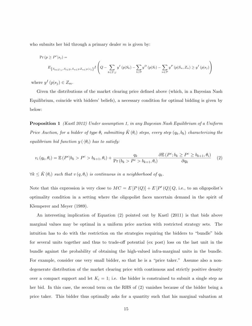
Proposition 1 (Kastl 2012) Under assumption 1, in any Bayesian Nash Equilibrium of a Uniform
Price Auction, for a bidder of type θi submitting K (θi) steps, every step (qk, bk) characterizing the
equilibrium bid function y (·|θi) has to satisfy:
vi (qk, θi) = E (P c|bk > P c > bk+1, θi) +qk
Pr (bk > P c > bk+1, θi)
∂E (P c; bk ≥ P c ≥ bk+1, θi)
∂qk(2)
∀k ≤ K (θi) such that v (q, θi) is continuous in a neighborhood of qk.
Note that this expression is very close to MC = E [P (Q)] + E [P ′ (Q)]Q, i.e., to an oligopolist’s
optimality condition in a setting where the oligopolist faces uncertain demand in the spirit of
Klemperer and Meyer (1989).
An interesting implication of Equation (2) pointed out by Kastl (2011) is that bids above
marginal values may be optimal in a uniform price auction with restricted strategy sets. The
intuition has to do with the restriction on the strategies requiring the bidders to “bundle” bids
for several units together and thus to trade-off potential (ex post) loss on the last unit in the
bundle against the probability of obtaining the high-valued infra-marginal units in the bundle.
For example, consider one very small bidder, so that he is a “price taker.” Assume also a non-
degenerate distribution of the market clearing price with continuous and strictly positive density
over a compact support and let Ki = 1; i.e. the bidder is constrained to submit a single step as
her bid. In this case, the second term on the RHS of (2) vanishes because of the bidder being a
price taker. This bidder thus optimally asks for a quantity such that his marginal valuation at
15
that quantity is equal to the expected price conditional on this price being lower than his bid, i.e.
vi (qk, θi) = E (P c|bk > P c, θi). Therefore, whenever there is a positive probability of the market
clearing price being below his bid, his bid will be higher than his marginal valuation for that
quantity.
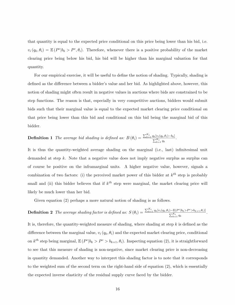
For our empirical exercise, it will be useful to define the notion of shading. Typically, shading is
defined as the difference between a bidder’s value and her bid. As highlighted above, however, this
notion of shading might often result in negative values in auctions where bids are constrained to be
step functions. The reason is that, especially in very competitive auctions, bidders would submit
bids such that their marginal value is equal to the expected market clearing price conditional on
that price being lower than this bid and conditional on this bid being the marginal bid of this
bidder.
Definition 1 The average bid shading is defined as: B (θi) =∑Ki
k=1 qk[vi(qk,θi)−bk]∑Kik=1 qk
.
It is thus the quantity-weighted average shading on the marginal (i.e., last) infinitesimal unit
demanded at step k. Note that a negative value does not imply negative surplus as surplus can
of course be positive on the inframarginal units. A higher negative value, however, signals a
combination of two factors: (i) the perceived market power of this bidder at kth step is probably
small and (ii) this bidder believes that if kth step were marginal, the market clearing price will
likely be much lower than her bid.
Given equation (2) perhaps a more natural notion of shading is as follows.
Definition 2 The average shading factor is defined as: S (θi) =∑Ki
k=1 qk[vi(qk,θi)−E(P c|bk>P c>bk+1,θi)]∑Kik=1 qk
.
It is, therefore, the quantity-weighted measure of shading, where shading at step k is defined as the
difference between the marginal value, vi (qk, θi) and the expected market clearing price, conditional
on kth step being marginal, E (P c|bk > P c > bk+1, θi). Inspecting equation (2), it is straightforward
to see that this measure of shading is non-negative, since market clearing price is non-decreasing
in quantity demanded. Another way to interpret this shading factor is to note that it corresponds
to the weighted sum of the second term on the right-hand side of equation (2), which is essentially
the expected inverse elasticity of the residual supply curve faced by the bidder.
16
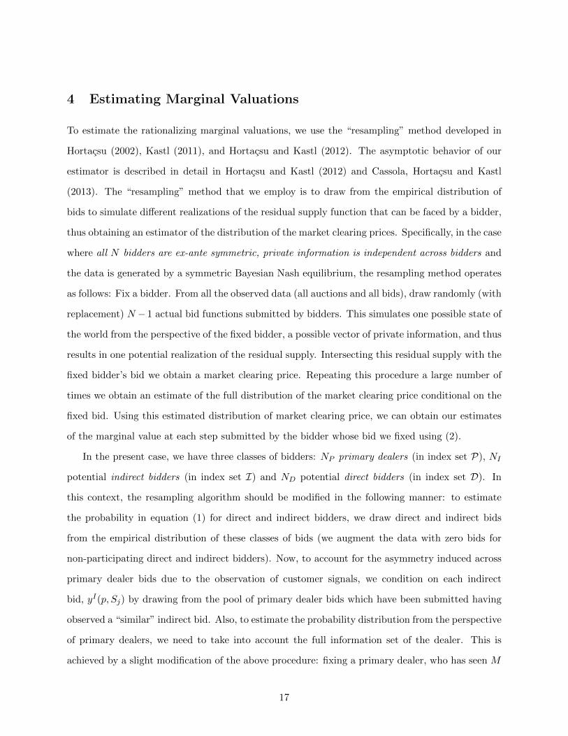
4 Estimating Marginal Valuations
To estimate the rationalizing marginal valuations, we use the “resampling” method developed in
Hortacsu (2002), Kastl (2011), and Hortacsu and Kastl (2012). The asymptotic behavior of our
estimator is described in detail in Hortacsu and Kastl (2012) and Cassola, Hortacsu and Kastl
(2013). The “resampling” method that we employ is to draw from the empirical distribution of
bids to simulate different realizations of the residual supply function that can be faced by a bidder,
thus obtaining an estimator of the distribution of the market clearing prices. Specifically, in the case
where all N bidders are ex-ante symmetric, private information is independent across bidders and
the data is generated by a symmetric Bayesian Nash equilibrium, the resampling method operates
as follows: Fix a bidder. From all the observed data (all auctions and all bids), draw randomly (with
replacement) N −1 actual bid functions submitted by bidders. This simulates one possible state of
the world from the perspective of the fixed bidder, a possible vector of private information, and thus
results in one potential realization of the residual supply. Intersecting this residual supply with the
fixed bidder’s bid we obtain a market clearing price. Repeating this procedure a large number of
times we obtain an estimate of the full distribution of the market clearing price conditional on the
fixed bid. Using this estimated distribution of market clearing price, we can obtain our estimates
of the marginal value at each step submitted by the bidder whose bid we fixed using (2).
In the present case, we have three classes of bidders: NP primary dealers (in index set P), NI
potential indirect bidders (in index set I) and ND potential direct bidders (in index set D). In
this context, the resampling algorithm should be modified in the following manner: to estimate
the probability in equation (1) for direct and indirect bidders, we draw direct and indirect bids
from the empirical distribution of these classes of bids (we augment the data with zero bids for
non-participating direct and indirect bidders). Now, to account for the asymmetry induced across
primary dealer bids due to the observation of customer signals, we condition on each indirect
bid, yI(p, Sj) by drawing from the pool of primary dealer bids which have been submitted having
observed a “similar” indirect bid. Also, to estimate the probability distribution from the perspective
of primary dealers, we need to take into account the full information set of the dealer. This is
achieved by a slight modification of the above procedure: fixing a primary dealer, who has seen M
17
indirect bids, we draw NI −M , rather than NI , indirect bids, and take the observed indirect bid
along with the dealer’s own bid as given when calculating the market clearing price, i.e., we subtract
the actual observed customer bid from the supply before starting the resampling procedure.
It is worth stressing that the above-described resampling method rests heavily on the assump-
tion of ex-ante within group symmetry of primary dealers, direct and indirect bidders, and condi-
tional (on auction level observables) independence of private information. Unobserved heterogeneity
across auctions that may be driving valuations is a big concern in the empirical auctions literature.
The danger this creates is the potential pooling of bidding data across auctions that have very dif-
ferent demand structures, which will cloud inference regarding the probability distribution of the
market clearing price. Another, related, concern is the potential for multiple strategic equilibria –
bidders may be playing different equilibria in different auctions in the data set. To combat these
issues, we use marginal valuations auction-by-auction; using data on bids from only one auction at
a time. While this reduces precision of our estimates, the volatile economic environment especially
in 2009 and 2010 suggests that auctions of the same security at different times may be subject to
very different demand-side factors and that accounting for unobservables at the auction level may
be very important. We discuss the consistency property of the single-auction estimation scheme in
Cassola, Hortacsu and Kastl (2013).
Using this modified resampling method we can therefore obtain an estimate of the distribution
of market clearing price from the perspective of each bidder. Inspecting equation (2), the only
other object we need to estimate is the slope of the unconditional expectation. We estimate this
using the standard numerical derivative approach. In particular, for each bidder we use the same
resampling approach described earlier to estimate E (P c|bk ≥ P c ≥ bk+1), which together with an
estimate of Pr (bk ≥ P c ≥ bk+1) and Bayes’ rule yields an estimate of E (P c; bk ≥ P c ≥ bk+1). Call
this estimate ERT (P c; bk ≥ P c ≥ bk+1), where T indexes the sample size (the number of auctions)
and R stands for the resampling estimator. To obtain an estimate of the numerical derivative
of this expectation with respect to quantity demanded at step k we perturb qk in the submitted
bid vector to some qk − εd and obtain an estimate of ERT (P c; bk ≥ P c ≥ bk+1) conditional on the
18
perturbed bid vector. We can then construct the estimator of the derivative:
∂ERT (P c; bk ≥ P c ≥ bk+1)
∂qk=
ERT (P c; bk ≥ P c ≥ bk+1, qk)− ERT (P c; bk ≥ P c ≥ bk+1, qk − εd)εd
where {εd}∞d=1 is a sequence converging to zero. One difficulty when estimating the slope of this
expectation w.r.t. qk is choosing the appropriate neighborhood εd so that the numerical derivative
is a consistent estimate. Loosely speaking, this neighborhood should shrink to zero as the sample
size increases. Pakes and Pollard (1989) establish that with a regularity condition (on uniformity),
such an estimator is consistent whenever T−12 ε−1 = Op (1), i.e., whenever ε does not decrease too
fast as the sample size increases.
5 Results
5.1 Bid Shading Analysis
As we discussed in our analysis of bids, the difference in bids across bidder groups may arise from
two separate factors: differential ability to exercise market power, i.e. bid shading, vs. differential
willingness-to-pay for the issued security. Our estimation method yields estimates of the two terms
on the right hand side of Equation (2) based on the empirical distribution of bids within each
auction in our data set. Using these, we can construct an estimate of the marginal valuation for
each bid step, which can then be utilized to compute the two different shading factors we defined
in the previous section for each bidder and auction.
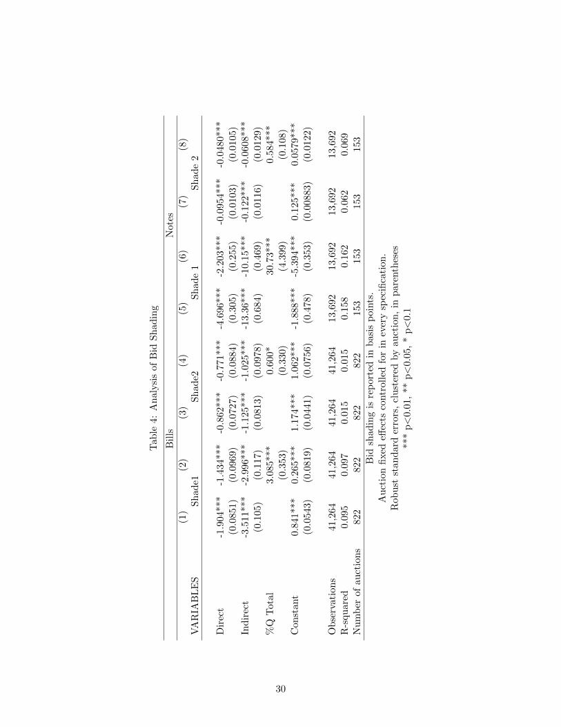
Table 4 reports the results of regressions similar to those for bids. The first two columns of the
table look at the differences in bid shading (according to Definition 1 above) across bidder groups
for the Bill sector. Column (1) implies that Primary Dealers shade their bids 1.9 basis points more
than Direct Bidders, and 3.5 basis points higher than Indirect Bidders. Column (2) introduces the
bidder size control, and we find that the shading differentials decline slightly, to 1.4 basis point
against Direct Bidders and 3 basis points against Indirect Bidders. We also find, intuitively, that
larger bidders choose to shade their bids more. The coefficient estimate suggests that going from
zero to 10% market share allows a dealer to shade her bids by 0.3 basis points.
19

Columns (3) and (4) repeat the same analysis for Definition 2 of bid shading, and find qualita-
tively the same result.
Columns (5) through (8) repeat the analysis for the Notes sector. Here, we see even larger
differentials in shading. Primary Dealers shade their bids (according to Definition 1) 5 basis points
more than Direct Bidders and 13 basis points more than Indirect Bidders. Putting in the control
for bidder size, once again we find that larger bidders can shade their bids more: going from zero
to 10% market share increases shading by 3 basis points. The size control diminishes the shading
differential between Primary Dealers and Direct and Indirect Bidders (to 2 and 10 basis points),
but, once again, does not eliminate the differential. Once again, Columns (7) and (8) repeat the
analysis with the second definition of bid shading. The qualitative results are the same as for the
Definition 1.
Demand Differentials or Bid-Shading Differentials?
Recall that our analysis of bids in Table 3 revealed that, controlling for size, Primary Dealers
bid 1 (2.5) basis points higher yields than Direct(Indirect) bidders for Bills, and 1 (4) basis points
higher yields for Notes. Since we found that Primary Dealers shade their bids 1.4 (3) basis points
more than Direct (Indirect) for Bills, and 2(10) basis points more than Direct (Indirect) bidders
for Notes, the bid differentials are rationalized by Primary Dealers having 0.4 (0.5) basis points
higher willingness-to-pay for Bills, and 1 (6) basis points higher willingness-to-pay for Notes – again,
controlling for bidder size. I.e., our results suggest that, under the assumption of expected profit
maximization, the main reason why Primary Dealers bid higher yields than other bidder groups is
not because they have lower valuation for the securities, but because they are able to exercise more
market power.
5.2 Infra-marginal Surplus Analysis
A question related to bid-shading that we can answer through our analysis is to quantify how much
infra-marginal surplus bidders are getting from participating in these auctions. Once again, we
can utilize Equation (2) to calculate the bidders’ marginal valuations, and use these to compute
ex-post surplus each bidder gains on the units that they win in the auction. To compute surplus, we
20
obtain point estimates of the “rationalizing” marginal valuation function v (q, s) at the (observed)
quantities that the bidders request. We then compute the area under the upper envelope of the
inframarginal portion of the marginal valuation function, and subtract the payment made by each
bidder.
We should provide abundant caution that “infra-marginal bidder surplus” does not reflect the
“cost” of running the auction system. Any counterfactual auction system would also have to allow
bidders to retain some surplus. Indeed, in Figure 1, we see very clearly that even if bidders bid
perfectly competitively, i.e. reveal their true marginal valuations without any bid shading, they
would gain some surplus from the auction, just because they have downward sloping demand curves.
At best, what we can say is that the bidder surpluses we compute here reflect an upper bound to
the amount of cost-saving that can be induced by a change in issuance mechanism.
Moreover, the surpluses we calculate here may significantly exceed the simple trading profits
that some bidders, especially Primary Dealers, may derive from reselling the securities. Retaining
Primary Dealership status has a number of complementary value streams attached to it beyond
the profits derived from reselling the new issues. For example, being a Primary Dealer allows firms
access to open market operations and, especially in this period, the QE auction mechanism that is
exclusive to primary dealerships. Between March 2008 and February 2010, Primary Dealers also
had access to a special credit facility from the Fed to help alleviate liquidity constraints during the
crisis. Indeed, compared to Primary Dealers, we may expect the surpluses attained by Direct and
Indirect bidders to be more closely aligned with their outside options of purchasing these securities
from secondary markets.
With the above qualifications, Table 5 reports the infra-marginal surpluses enjoyed by different
bidders groups across the maturity spectrum. We report the surpluses in basis points, and also
report the total infra-marginal surpluses accrued to the bidders during our sample period of July
2009 to October 2013.
Direct and Indirect bidder surpluses are between 0.02 and 3.58 basis points across the maturity
spectrum, with the shorter end of the maturity spectrum generating very low surpluses in general.
Once again, these surpluses may reflect the outside option of not buying these securities in auction
21
and purchasing them in the when-issued or resale markets – and appear sensible given the differen-
tials between auction prices and secondary market rates. Aggregating the surpluses over the entire
set of auctions in our data set (which amounted to about $27 trillion in issue size), we find Direct
and Indirect Bidders’ aggregate surplus to be about $1.6 billion, or about 0.6 basis points.
Primary Dealers’ infra-marginal surplus, however, appears to be significantly larger. As we
noted above, for Primary Dealers, the derived surplus might not necessarily be in line with the
differentials with the quoted secondary market prices of these securities: first of all, Primary
Dealers’ demand is typically quite large, and fulfilling such levels of demand is likely to have a
price impact in the secondary markets. Moreover, consistently winning some of the issuance in the
auctions is necessary to maintain primary dealership status, which has additional value streams
attached to it.
We find that Primary Dealers derive most of their infra-marginal surplus from the longer end (2
to 10 year notes) of the maturity spectrum. There may be a number of reasons why demand for this
part of the maturity spectrum is more heterogenous across bidders. One possibility is the presence
of different portfolio needs across dealers’ clientele. Moreover, there are typically alternative uses
for such securities beyond simple buy-and-hold – Duffie (1996) shows that this part of the spectrum
can be particularly valuable for its use as collateral in repo transactions. Surpluses derived from
the shorter end of the maturity spectrum, which may have fewer alternative uses, are much smaller.
Overall, we find that Primary Dealers’ derived surplus aggregated to $6.3 billion during our
sample period. Compared against the $27 trillion in issuance, Primary Dealer surplus makes up
for 2.3 basis points of the issuance. Along with the Direct Bidder and Indirect Bidder surpluses,
we find that bidder surplus added up to 3 basis points during this period.
Once again, the surpluses we report here do not necessarily reflect the “cost of issuance.” Any
other issuance mechanism would have to provide bidders with surpluses to ensure participation and
to reward them for their private information. Moreover, even if bidders are behaving as if they
were perfectly competitive, they would enjoy surpluses. However, we can conservatively estimate
that revenue gains from further optimizing the issuance mechanism is bounded above by 3 basis
points.
22
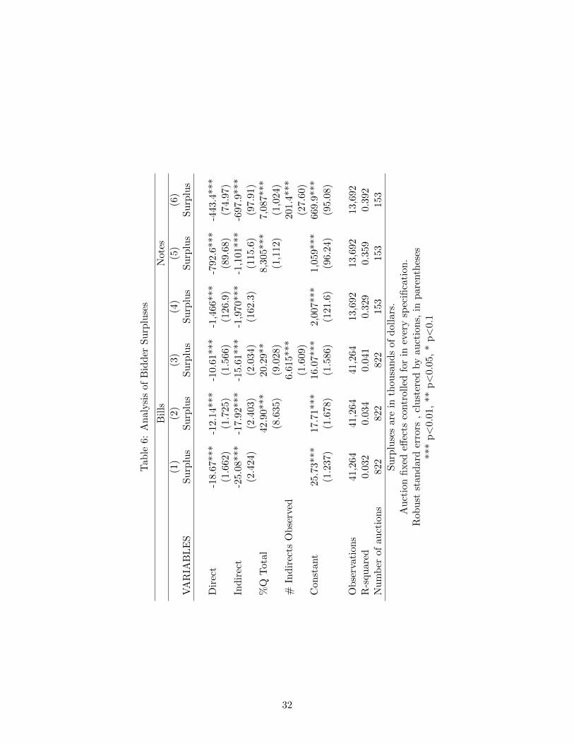
Table 6 runs regressions on the calculated bidder surpluses that closely resemble those in Tables 3
and 4. The surpluses here are reported in thousands of dollars, and all regressions control for auction
fixed effects, giving us within auction comparisons. In Column (1), we find that Direct and Indirect
bidders gain significantly lower surpluses than Primary Dealers (the excluded category appearing
in the constant), and that Indirect bidder surplus especially is not statistically different from zero.
Column (2) adds in the bidder size control, measured as the bidder’s tender size as percentage
of total supply (% Q Total). We find that larger bidders indeed gain higher surpluses. However,
Direct and Indirect Bidders gain lower surpluses than Primary Dealers even when size is controlled
for.
Column (3) introduces a new control variable – we have added here the number of Indirect
Bidders whose bids a Primary Dealer routes in the auction. This variable is a rough proxy for
the order-flow information that the Primary Dealer is privy to. Indeed, the regression reveals a
significant correlation between the number of Indirect Bidders who routed their bids through a
Primary Dealer, and the surplus (controlling for the bidder’s size). An additional Indirect Bidder
going through a Primary Dealer would be correlated with about seven thousand dollars more in
surplus.
Columns (4) through (6) repeat the same analysis for the Notes sector. We note that the implied
Primary Dealer surplus in this sector (which is measured by the constant term in our regression) is
much larger as compared to their surplus in Bills auctions. Direct and Indirect Bidders gain much
smaller surpluses compared to the Primary Dealers – indeed, Indirect Bidder surplus is very close
to zero.
When we control for bidder size in Column (5), we find a very large benefit to being large.
An increase in market share from 0 to 10% of the issue size is correlated with a rise in surplus of
$830k in the Notes auctions. Once again, though, we should stress that this is not necessarily due
to market power. It is very possible that larger bidders also have higher demand, and thus derive
more surplus from the auctions.
Finally, we introduce the number of Indirect Bidders routed by Primary Dealers in Column
(6). Here, we find that each additional Indirect Bidder observed is associated with a $200K gain
23
in Primary Dealer surplus. Since Primary Dealers on average route 2.5 Indirect Bids in Notes
auctions, this estimate suggests that we can ascribe about $500K or about 25% of their surplus
in Notes auctions to information contained in Indirect bids. However, we should note that there
are important caveats to interpreting this as the “value of order flow.” It is possible that Primary
Dealers who observe more Indirect bids may have systematically higher valuations for the securities,
and hence may be getting higher surpluses due to this.7
6 Conclusion
We have analyzed a unique and detailed data set to study bidding behavior in a large sample
of U.S. Treasury auctions conducted between July 2009 and October 2013. We have documented
significant differences in bidding behavior across the three different bidder groups: Primary Dealers,
Direct Bidders, and Indirect Bidders. We provide a modelling framework to decompose the bidding
differentials into differences in demand/willingness to pay, and differences in ability to exercise
market power. We estimate market power by assuming rational expectations about the elasticity
of residual supply. Our results suggest that opportunities to exercise market power do exist in this
market, and that Primary Dealers especially have the potential to shade their bids significantly – to
the extent that their bids are lower (higher yield) than others, even though their willingness-to-pay
is higher.
We also quantify the bidder surpluses that rationalize observed bids within our model. We
estimate total bidder surplus to be about 3 basis points of the total issue size, with higher surpluses
in Treasury Notes auctions as compared to Treasury Bills auctions. Under the assumption that the
mechanism is achieving an approximately efficient allocation, 3 basis points is also a conservative
upper bound on the amount of cost-savings that the Treasury can gain from optimizing its issuance
mechanism.
7In our prior work on Canadian Treasury auctions (Hortacsu and Kastl (2012)) we focused on revisions of primarydealers upon getting indirect bid information. This way, we were able to conduct a “but-for” analysis of how indirectbids contribute to primary dealers’ surplus. Unfortunately, in this context, we do not observe bid revisions – thoughwe should note that in the Canadian context we found that customer/indirect bids made up between 13-27% ofprimary dealer surplus, which is close to the 25% estimate we are getting here.
24
References
Ausubel, Lawrence and Peter Cramton, “Demand Reduction and Inefficiency in Multi-Unit
Auctions,” 2002. working paper.
Cassola, Nuno, Ali Hortacsu, and Jakub Kastl, “The 2007 Subprime Market Crisis in the
EURO Area Through the Lens of ECB Repo Auctions,” Econometrica, 2013, 81 (4), pp.
1309–1345.
Duffie, Darrell, “Special Repo Rates,” The Journal of Finance, 1996, 51 (2), pp. 493–526.
Elyakime, Bernard, Jean-Jacques Laffont, Patrice Loisel, and Quang Vuong, “Auc-
tioning and Bargaining: An Econometric Study of Timber Auctions with Secret Reservation
Prices,” Journal of Business & Economic Statistics, April 1997, 15 (2), pp.209–220.
Fleming, Michael, “Who Buys Treasury Securities at Auction?,” Current Issues in Economics
and Finance, 2007, 13, Federal Reserve Bank of New York.
and Joshua V. Rosenberg, “How Do Treasury Dealers Manage Their Positions?,” August
2007. Federal Reserve Bank of New York Staff Reports, No. 299.
Friedman, Milton, A Program For Monetary Stability, Fordham University Press, 1960.
Garbade, Kenneth D., “Why the U.S. Treasury Began Auctioning Treasury Bills in 1920,”
Economic Policy Review, 2008, 14, Federal Reserve Bank of New York.
and Jeffrey Ingber, “The Treasury Auction Process: Objectives, Structure, and Recent
Adaptations,” Current Issues in Economics and Finance, 2005, p. Federal Reserve Bank of
New York.
, John Partlan, and Paul Santoro, “Recent Innovations in Treasury Cash Management,”
Current Issues in Economics and Finance, 2004, 10, Federal Reserve Bank of New York.
Guerre, Emmanuel, Isabelle Perrigne, and Quang Vuong, “Optimal Nonparametric Esti-
mation of First-Price Auctions,” Econometrica, 2000, 68 (3), pp. 525–574.
25
Hortacsu, Ali, “Mechanism Choice and Strategic Bidding in Divisible Good Auctions: An Em-
pirical Analysis of the Turkish Treasury Auction Market,” 2002. working paper.
and David McAdams, “Mechanism Choice and Strategic Bidding in Divisible Good Auc-
tions: An Empirical Analysis of the Turkish Treasury Auction Market,” Journal of Political
Economy, 2010, 118 (5), pp. 833–865.
and Jakub Kastl, “Valuing Dealers’ Informational Advantage: A Study of Canadian Trea-
sury Auctions,” Econometrica, 2012, 80 (6), pp.2511–2542.
Kastl, Jakub, “Discrete Bids and Empirical Inference in Divisible Good Auctions,” Review of
Economic Studies, 2011, 78, pp. 978–1014.
, “On the Properties of Equilibria in Private Value Divisible Good Auctions with Constrained
Bidding,” Journal of Mathematical Economics, 2012, 48 (6), pp. 339–352.
Klemperer, Paul and Margaret Meyer, “Supply function equilibria in oligopoly under uncer-
tainty,” Econometrica, 1989, 57 (6), pp.1243–1277.
Laffont, Jean-Jacques and Quang Vuong, “Structural Analysis of Auction Data,” The Amer-
ican Economic Review, 1996, 86 (2), pp. 414–420.
Malvey, Paul and Christine Archibald, “Uniform Price Auctions: Update of the Treasury
Experience,” 1998.
Pakes, Ariel and David Pollard, “Simulation and the Asymptotics of Optimization Estimators,”
Econometrica, 1989, 57 (5), pp.1027–1057.
Ramanathan, Karthik, “Overview of U.S. Treasury Debt Management,” 2008.
Wilson, Robert, “Auctions of Shares,” The Quarterly Journal of Economics, 1979, 93 (4), pp.
675–689.
26

Tab
le1:
Su
mm
ary
Sta
tist
ics
Pri
mar
yD
eale
rsD
irec
tB
idd
ers
Ind
irec
tB
idd
ers
Mat
uri
tyTa
Q($
bn
)b%
QTd
%Q
Ae
%Q
Td
%Q
Ae
%Q
Td
%Q
Ae
CM
Bsf
101
24.6
88%
76%
6%7%
6%17
%4
wee
k222
31.9
85%
65%
7%8%
8%27
%13
wee
k222
28.5
86%
67%
7%8%
7%25
%26
wee
k222
24.9
84%
61%
7%8%
9%31
%52
wee
k55
24.3
82%
61%
8%10
%10
%29
%2
yea
r51
34.7
73%
55%
13%
17%
14%
28%
5yea
r51
34.3
70%
48%
12%
12%
18%
40%
10yea
r51
20.5
69%
46%
13%
16%
18%
38%
aN
um
ber
of
auct
ions
bA
ver
age
issu
esi
zec
%of
the
tota
ldem
and
tender
ed.
d%
of
the
tota
lsu
pply
alloca
ted.
fC
ash
Managem
ent
Bills
27
Tab
le2:
Des
crip
tion
ofB
ids
Pri
mar
yD
eale
rsD
irec
tB
idd
ers
Ind
irec
tB
idd
ers
Matu
rity
Bida
SD
[Bid
]b%
QTc
%W
ind
Bid
SD
[bid
]%
QT
%W
inB
idB
id%
QT
%W
inC
MB
s0.
1501
0.0
244
19%
21%
0.13
890.
0201
5%36
%0.
1185
0.02
233%
64%
4w
eek
0.0
943
0.02
5418
%19
%0.
0699
0.03
373%
52%
0.04
630.
0266
2%84
%13
wee
k0.1
119
0.0
248
19%
19%
0.08
660.
0332
3%54
%0.
0683
0.02
492%
84%
26w
eek
0.165
0.0
275
20%
16%
0.13
680.
0391
4%52
%0.
1254
0.02
722%
71%
52w
eek
0.2
617
0.0
299
17%
20%
0.23
560.
0333
4%47
%0.
227
0.01
72%
67%
2yea
r0.5
604
0.03
9713
%22
%0.
5231
0.04
64%
42%
0.49
270.
0939
1%70
%5
yea
r1.5
627
0.06
8210
%24
%1.
4902
0.06
313%
55%
1.43
840.
1244
1%82
%10
yea
r2.7
229
0.07
3211
%21
%2.
6482
0.07
063%
50%
2.59
060.
192
1%71
%a
Aver
age
quanti
ty-w
eighte
dbid
-yie
ldacr
oss
auct
ions
bA
ver
age,
acr
oss
auct
ions,
of
wit
hin
auct
ion
standard
dev
iati
on
of
quanti
ty-w
eighte
dbid
-yie
ldc
The
%of
tota
lquanti
tydem
and
by
abid
der
,av
eraged
acr
oss
auct
ions
d%
of
the
quanti
tydem
anded
by
bid
der
that
was
won
inth
eauct
ion,
aver
aged
acr
oss
auct
ions
28

Table 3: Analysis of Bids
Bills Notes
(1) (2) (3) (4)Dep. Var. QwBid(bp) QwBid(bp) QwBid(bp) QwBid(bp)
Direct -2.457*** -0.929*** -5.974*** -0.965***(0.0580) (0.0600) (0.270) (0.314)
Indirect -4.204*** -2.529*** -10.89*** -4.437***(0.0604) (0.0613) (0.356) (0.399)
%Q Total 10.04*** 61.75***(0.219) (5.452)
Constant 13.87*** 11.99*** 172.0*** 165.0***(0.0316) (0.0426) (0.261) (0.460)
Observations 41,359 41,359 13,692 13,692R-squared 0.254 0.289 0.086 0.099Number of auctions 822 822 153 153
Bids reported in units of basis points.Auction fixed effects controlled for.
Robust standard errors, clustered at auction level, in parentheses*** p<0.01, ** p<0.05, * p<0.1
29
Tab
le4:
An
alysi
sof
Bid
Sh
adin
g
Bil
lsN
otes
(1)
(2)
(3)
(4)
(5)
(6)
(7)
(8)
VA
RIA
BL
ES
Sh
ad
e1S
had
e2S
had
e1
Sh
ade
2
Dir
ect
-1.9
04**
*-1
.434
***
-0.8
62**
*-0
.771
***
-4.6
96**
*-2
.203
***
-0.0
954*
**-0
.048
0***
(0.0
851
)(0
.096
9)(0
.072
7)(0
.088
4)(0
.305
)(0
.255
)(0
.010
3)(0
.010
5)In
dir
ect
-3.5
11*
**-2
.996
***
-1.1
25**
*-1
.025
***
-13.
36**
*-1
0.15
***
-0.1
22**
*-0
.060
8***
(0.1
05)
(0.1
17)
(0.0
813)
(0.0
978)
(0.6
84)
(0.4
69)
(0.0
116)
(0.0
129)
%Q
Tot
al
3.08
5***
0.60
0*30
.73*
**0.
584*
**(0
.353
)(0
.330
)(4
.399
)(0
.108
)C
onst
ant
0.84
1***
0.2
65**
*1.
174*
**1.
062*
**-1
.888
***
-5.3
94**
*0.
125*
**0.
0579
***
(0.0
543
)(0
.081
9)(0
.044
1)(0
.075
6)(0
.478
)(0
.353
)(0
.008
83)
(0.0
122)
Ob
serv
atio
ns
41,
264
41,2
6441
,264
41,2
6413
,692
13,6
9213
,692
13,6
92R
-squ
ared
0.0
950.
097
0.01
50.
015
0.15
80.
162
0.06
20.
069
Nu
mb
erof
au
ctio
ns
822
822
822
822
153
153
153
153
Bid
shad
ing
isre
por
ted
inb
asis
poi
nts
.A
uct
ion
fixed
effec
tsco
ntr
olle
dfo
rin
ever
ysp
ecifi
cati
on.
Rob
ust
stan
dar
der
rors
,cl
ust
ered
by
auct
ion
,in
par
enth
eses
***
p<
0.01
,**
p<
0.05
,*
p<
0.1
30

Table 5: Bidder surpluses: July 2009-October 2013
PD Surplus DB Surplus IB Surplus
Maturity (bp) (M$) (bp) (M$) (bp) (M$)
CMBs 0.17 40.6 0.02 3.8 0.04 9.64-Week 0.04 26.2 0.00 2.1 0.002 1.1
13-Week 0.13 86.4 0.02 11.1 0.008 5.326-Week 0.33 183 0.03 15.1 0.026 14.652-Week 0.68 90.8 0.08 10.5 0.14 18.4
2-Year 7.40 1310 1.15 202 0.91 1615-Year 13.07 2280 1.87 326 1.39 243
10-Year 22.22 2320 3.58 373 1.73 180
Overall 2.3 6337 0.35 943.5 0.23 633
31
Tab
le6:
An
alysi
sof
Bid
der
Su
rplu
ses
Bil
lsN
otes
(1)
(2)
(3)
(4)
(5)
(6)
VA
RIA
BL
ES
Su
rplu
sS
urp
lus
Su
rplu
sS
urp
lus
Su
rplu
sS
urp
lus
Dir
ect
-18.
67**
*-1
2.14
***
-10.
61**
*-1
,466
***
-792
.6**
*-4
43.4
***
(1.6
62)
(1.7
25)
(1.5
66)
(126
.9)
(89.
68)
(74.
97)
Ind
irec
t-2
5.08
***
-17.
92**
*-1
5.61
***
-1,9
70**
*-1
,101
***
-697
.9**
*(2
.424
)(2
.403
)(2
.034
)(1
62.3
)(1
15.6
)(9
7.91
)%
QT
otal
42.9
0***
20.2
9**
8,30
5***
7,08
7***
(8.6
35)
(9.0
28)
(1,1
12)
(1,0
24)
#In
dir
ects
Ob
serv
ed6.
615*
**20
1.4*
**(1
.609
)(2
7.60
)C
onst
ant
25.7
3***
17.7
1***
16.0
7***
2,00
7***
1,05
9***
669.
9***
(1.2
37)
(1.6
78)
(1.5
86)
(121
.6)
(96.
24)
(95.
08)
Ob
serv
atio
ns
41,2
6441
,264
41,2
6413
,692
13,6
9213
,692
R-s
qu
ared
0.03
20.
034
0.04
10.
329
0.35
90.
392
Nu
mb
erof
au
ctio
ns
822
822
822
153
153
153
Su
rplu
ses
are
inth
ousa
nd
sof
dol
lars
.A
uct
ion
fixed
effec
tsco
ntr
olle
dfo
rin
ever
ysp
ecifi
cati
on.
Rob
ust
stan
dar
der
rors
,cl
ust
ered
by
auct
ion
s,in
par
enth
eses
***
p<
0.01
,**
p<
0.05
,*
p<
0.1
32