bias-free rainfall forecast and temperature trend-based ...eder/artigos/bias/bhardwaj_2007.pdf ·...

METEOROLOGICAL APPLICATIONSMeteorol. Appl. 14: 351–360 (2007)Published online 16 October 2007 in Wiley InterScience(www.interscience.wiley.com) DOI: 10.1002/met.35

Bias-free rainfall forecast and temperature trend-basedtemperature forecast using T-170 model output during the

monsoon season

Rashmi Bhardwaj,b* Ashok Kumar,a Parvinder Maini,a S.C. Kara and L.S. Rathorea

a National Center for Medium Range Weather Forecasting, A-50, Institutional Area Phase-II, Sector-62, NOIDA,UP,PIN:-201307b Department of Mathematics, Guru Gobind Singh Indraprastha University, Kashmere gate, Delhi-110006

ABSTRACT: An objective forecasting system for medium-range location-specific forecasting of surface weather elementshas been evolved at the National Centre for Medium Range Weather Forecasting, India (NCMRWF). The basic informationused for this is the output from the T-170 general circulation model (GCM). The direct model output (DMO) forecast isbriefly explained along with the T-170 model. The two important weather parameters considered in detail are rainfall andtemperature. Both the parameters have biases. Techniques used for obtaining bias-free rainfall forecasts and temperaturetrend-based forecasts are explained in detail. These forecasts are obtained for all of the 602 districts of India. Finally, anevaluation of the accuracy of rainfall and temperature forecasts for selected districts for which the observed data could beobtained during the 2006 monsoon is presented. Copyright 2007 Royal Meteorological Society

KEY WORDS NCMRWF; GCM; T-170 model; DMO; bias free

Received 5 December 2006; Revised 25 June 2007; Accepted 31 July 2007

1. Introduction

Historically, a weather forecast in India was mainlyissued in qualitative terms with the use of conventionalmethods assisted by satellite data and synoptic informa-tion for the location of interest. These forecasts weresubjective and could not be used for risk assessment inquantitative terms. Hence, work was initiated to developan objective medium-range local weather forecasting sys-tem in India in 1988 at the National Centre for MediumRange Weather Forecasting (NCMRWF). An R-40 gen-eral circulation model with a resolution of 2.8° × 1.8°

was installed for this purpose in 1989 and a T-80 generalcirculation model with a higher resolution of 1.5° × 1.5°

was made operational in 1993. In 2002, a T-170 generalcirculation model with a still higher resolution 0.7° × 0.7°

was made experimentally operational.An objective forecast is a forecast that does not depend

on the subjective judgement of the person issuing it.Strictly speaking, an objective forecasting system isone that can produce one and only one forecast froma specific set of data. The objective forecast for theabove surface parameters is directly obtained from thegeneral circulation model operational at NCMRWF andis called the direct model output (DMO) forecast, asthis forecast has the biases and systematic errors of thegeneral circulation model. The work for removing biasesand systematic errors from the most important weather

* Correspondence to: Rashmi Bhardwaj, Department of Mathematics,Guru Gobind Singh Indraprastha University, Kashmere gate, Delhi-110006. E-mail: rb [email protected]

parameters has been undertaken. These forecasts areused operationally at NCMRWF for providing the finallocal weather forecast for these parameters at differentlocations. In the present paper, the bias-free DMOforecast using T-170 model output is explained in detail.

In Section 2, the T-170 model and the forecast for theimportant surface weather elements, which are directlyobtained from the numerical weather prediction (NWP)model, are explained. In Section 3, the bias-free rainfallforecast is presented. Section 4 discusses the temperatureforecast based on temperature trends in detail. Section5 describes the evaluation of the forecast skill for thebias-free rainfall forecast and trend-based temperatureforecast.

2. T-170 model and direct model output (DMO)forecast

2.1. T-170 model

The NCMRWF T-170/L28 global spectral model wasdeveloped in-house (Kar, 2002). It was based on theNCEP T80/L18 model (Kanamitsu, 1989; Kalnay et al.,1990; Kanamitsu et al., 1991) and subsequent changeswere made to the T80/L18 model at NCMRWF. Atmo-spheric dynamics were based on primitive equations withvorticity, divergence, logarithm of surface pressure, spe-cific humidity and virtual temperature as dependent vari-ables.

In this model, horizontal representation is spectral(spherical harmonic basis functions) with transformation

Copyright 2007 Royal Meteorological Society

352 RASHMI BHARDWAJ ET AL.

Table I. Brief description of T-170/L28 global spectral model.

Modelelements

Components Specifications

Grid Horizontal Global spectral-T-170 (512 × 256)Vertical 28 Sigma layers [F = 0.995, 0.982, 0.964, 0.942, 0.915, 0.883, 0.845,

0.801, 0.750, 0.693, 0.632, 0.568, 0.501, 0.435, 0.372, 0.312, 0.258, 0.210,0.168, 0.132, 0.102, 0.078, 0.058, 0.041, 0.028, 0.017, 0.009, 0.002]

Topography MEANDynamics Prognostic variables Relative vorticity, divergence, virtual temp., log of surface pressure, water

vapour mixing ratioHorizontal transform Orszag’s techniqueVertical differencing Arakawa’s energy-conserving schemeTime differencing Semi-implicit with 450 s of time stepTime filtering Robert’s methodHorizontal diffusion Second order over quasi-pressure surfaces, scale selective

Physics Surface fluxes Monin–Obukhov similarityTurbulent diffusion Non-local closureRadiation Short-wave: Harshvardhan et al. (NASA/Goddard)

Long-wave- Fels and SchwarzkopfDeep convection Kuo scheme modifiedShallow convection Tiedtke methodLarge-scale condensation Manabe-modified scheme based on saturationCloud generation Slingo schemeRainfall evaporation Kessler’s schemeLand surface processes Pan scheme having a three-layer soil model for soil temperature and bucket

hydrology of Manabe for soil moisture predictionAir–sea interaction Roughness length over sea computed by Charnock’s relation.

Climatological SST∗ , bulk formulae for sensible and latent heat fluxesGravity wave drag Lindzen and Pierrehumbert scheme

to a Gaussian grid for calculation of non-linear quantitiesand physics. The horizontal resolution is spectral triangu-lar truncation with 170 waves (T-170). In physical space,the horizontal resolution is of 512 × 256 grid size. This isroughly equivalent to 0.7° × 0.7° latitude/longitude gridspacing. The vertical domain is from the surface to about2.0 hPa, which is divided into 28 unequally spaced sigmalayers (Kar, 2002). For a surface pressure of 1000 hPa,the lowest atmospheric level is at a pressure of about995 hPa. The sigma layers in the model are representedas P/Ps, where P is the pressure at height at which thelayer is defined and Ps is surface pressure. The layersare located in such a way that near the surface and nearthe tropopause the layers are closely spaced compared tothe layers at other heights. This has been done to rep-resent the turbulence near the Earth’s surface and thetemperature gradient near the tropopause realistically.

The model has a comprehensive physics package,which includes parameterization schemes for cumu-lus convection, shallow convection, radiation, planetaryboundary layer, surface processes and gravity wave dragdue to mountains.

The time integration scheme is semi-implicit. Thetime step is 7.5 min for computation of the dynamicsand physics terms. However, full calculation of radia-tion (short-wave and long-wave) is done once every 6 h.This is to reduce computationally expensive full radiationcomputations. However, care has been taken to representthe diurnal cycle realistically by suitably interpolating

radiative heating and cooling to each time step. A com-plete description of the T-170 model is given in Tables Iand II (Kar, 2002).

2.2. Model output

From the 512 × 256 Gaussian grid points of the T-170model, an Indian window of size 50 × 50 grid (totalnumber of 2500 grid points) covering India is considered,

Table II. Specifications of initial surface boundary fields andcloud parameters.

Fields Land Ocean

Surface temperature Forecast ObservedSoil moisture Forecast NAAlbedo Climatology (S) Climatology (S)Snow cover Forecast ForecastRoughness length Climatology (S) ForecastPlant resistance Climatology (S) NASoil temperature Forecast NADeep soil temperature Climatology (A) NAConvective cloud cover Forecast ForecastConvective cloud bottom Forecast ForecastConvective cloud top Forecast ForecastSea ice NA Observed

(S) Seasonal.(A) Annual.NA Not Available.

Copyright 2007 Royal Meteorological Society Meteorol. Appl. 14: 351–360 (2007)DOI: 10.1002/met

BIAS-FREE RAINFALL FORECAST AND TREND-BASED TEMPERATURE FORECAST USING T-170 MODEL 353

starting at 38.9 °N latitude and 65.39 °E longitude to4.6 °N latitude and 100.55 °E longitude. For a particularday, 192 forecast values are obtained and the model isrun for 5 days starting from 0000 UTC initial conditions.

The model output is obtained at each time step at2500 grid points for the following six surface weatherelements.

• Surface pressure (hPa)• Rainfall rate (mm s−1)• Zonal wind component at 3.048 m (ms−1)• Meridional wind component at 3.048 m (ms−1)• Temperature at 1.3716 m (°C)• Specific humidity at 1.3716 m (g g−1)

The cloud amount (%) is obtained from the model at0000 UTC and 1200 UTC for each forecast day.

2.3. Interpolated forecast values

As the forecasts are obtained on the Gaussian grids andnot at a particular location, the simplest way to obtain aforecast at a specific location is to use the interpolatedvalue from the four grid points surrounding it. As thedistances between any two grid points of a 0.7° × 0.7°

grid window are not very large, the simple formulation ofthe Bessel interpolation formula is used for obtaining theforecast values of a particular station location (Figure 1)

2.4. Direct model output (DMO) forecast

DMO forecast values (interpolated) for each location ofinterest are obtained. A 4-day forecast for the followingparameters is obtained by using forecast values at eachtime step of 7.5 min.

• Average mean sea level pressure (hPa)• Cloud amount (morning and evening) (okta)• Rainfall (24 h accumulated) (mm)• Maximum temperature (°C)• Minimum temperature (°C)• Average wind speed (ms−1)• Predominant wind direction (°)• Maximum relative humidity (g g−1)• Minimum relative humidity (g g−1)

Interpolatedvalue at station

o o

o o o o

o o o o

o o o o

o o

O

Figure 1. Area considered around a station for getting interpolatedDMO forecast values.

Table III. State-specific HK scores attained and thresholdvalues for T-170 model forecast.

SN States/UT Order of theHK scores

attained

Thresholdrainfall

values (mm)

1 Andhra Pradesh 0.06–0.20 5.02 Assam 0.10–0.25 2.03 Arunachal Pradesh 0.08–0.26 2.04 Bihar 0.11–0.31 2.05 Chhattisgarh 0.20–0.43 2.06 Gujarat 0.25–0.46 0.57 Haryana 0.15–0.34 0.18 Himachal Pradesh 0.12–0.25 0.59 Jammu and Kashmir 0.10–0.20 0.5

10 Jharkhand 0.16–0.26 2.011 Karnataka 0.06–0.22 7.012 Kerala 0.08–0.15 7.013 Madhya Pradesh 0.24–0.49 1.014 Maharashtra 0.22–0.43 2.015 Manipur 0.10–0.23 2.016 Meghalaya 0.06–0.15 2.017 Mizoram 0.07–0.11 2.018 Nagaland 0.08–0.17 2.019 Orissa 0.15–0.34 2.020 Punjab 0.12–0.26 0.121 Rajasthan 0.21–0.39 0.122 Sikkim 0.09–0.16 2.023 Tamilnadu 0.05–0.26 5.024 Tripura 0.13–0.23 2.025 Uttaranchal 0.18–0.35 0.526 Uttar Pradesh 0.16–0.32 0.527 West Bengal 0.20–0.25 2.028 Delhi 0.40 0.129 Goa 0.26 2.030 Pondicherry 0.23 2.031 Lakshadweep 0.22 7.032 Daman and Diu 0.16 2.033 Dadra and Nagar 0.18 2.034 Chandigarh 0.29 0.135 Andaman and Nicobar 0.24 7.0

Here, the validity of the forecast values for a particularday is for the subsequent 24 h starting from 0300 UTC(0830 local time) of that day. As at the NCMRWF, theT-170 model is run only for 5 days based on 0000UTCanalysis, hence only the 24-, 48-, 72- and 96-h forecastscan be obtained.

2.5. Bias-free DMO forecast

To obtain a bias-free DMO forecast during any season,the forecast and observed values of the prediction duringthe recent one or two seasons are considered and correc-tion factors are obtained by a trial and error method sothat the skill of the forecast is maximized. The samecorrection factors are used while obtaining the bias-free DMO forecast during the current season. Duringthe present study, correction factors are calculated onthe basis of monsoon seasons (June, July, August andSeptember) of 2001, 2002 and 2003.



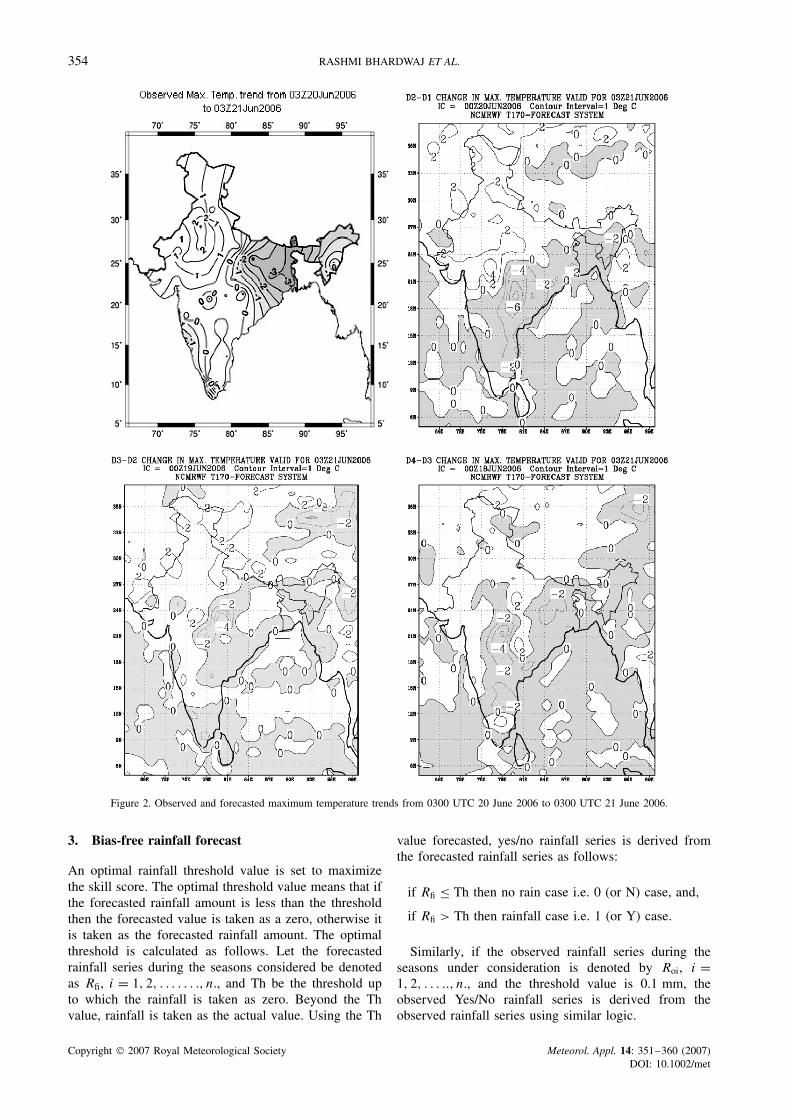
Figure 2. Observed and forecasted maximum temperature trends from 0300 UTC 20 June 2006 to 0300 UTC 21 June 2006.

3. Bias-free rainfall forecast

An optimal rainfall threshold value is set to maximizethe skill score. The optimal threshold value means that ifthe forecasted rainfall amount is less than the thresholdthen the forecasted value is taken as a zero, otherwise itis taken as the forecasted rainfall amount. The optimalthreshold is calculated as follows. Let the forecastedrainfall series during the seasons considered be denotedas Rfi, i = 1, 2, . . . . . . ., n., and Th be the threshold upto which the rainfall is taken as zero. Beyond the Thvalue, rainfall is taken as the actual value. Using the Th

value forecasted, yes/no rainfall series is derived fromthe forecasted rainfall series as follows:

if Rfi ≤ Th then no rain case i.e. 0 (or N) case, and,

if Rfi > Th then rainfall case i.e. 1 (or Y) case.

Similarly, if the observed rainfall series during theseasons under consideration is denoted by Roi, i =1, 2, . . . .., n., and the threshold value is 0.1 mm, theobserved Yes/No rainfall series is derived from theobserved rainfall series using similar logic.



Figure 3. Observed and forecasted minimum temperature trends from 0300 UTC 20 June 2006 to 0300 UTC 21 June 2006.

As scores used for verification of the rainfall forecastare the ratio score and Hanssen and Kuipers (HK) skillscore (Kumar et al., 2000), the ratio score measures thepercentage of correct forecasts out of the total forecastsissued. The HK skill score is the ratio of economic savingover climatology. Hence, the HK skill score is calculatedby using the observed and forecasted yes/no rainfall seriesbased on the data from the previous two to three seasons.The HK skill score is then maximized by varying thethreshold (Th) value used for deriving forecasted yes/norainfall series and the threshold value which maximizesthe HK Skill Score during previous seasons is appliedfor deriving the yes/no rainfall forecast from the DMO

rainfall forecast during the current season. The maximum

HK Skill Scores attained are given in Table III, and can

be explained by the following contingency table.

Forecasted Observed

Rain No Rain

Rain YY YNNo rain NY NN

Ratio Score = (YY + NN)/NHK skill score = (YY∗NN − YN∗NY)/(YY + YN)∗(NY + NN)



Figure 4. Observed and forecasted maximum temperature trends from 0300 UTC 10 July 2006 to 0300 UTC 11 July 2006.

If the HK skill score is closer to 1, the forecasts arebetter, and when the HK Score is near or less than 0 theforecasts are poorer.

In the present study, the rainfall threshold values arecalculated, and representative values are derived for thestations of each state of India. These values are given inTable III.

4. Temperature trend-based temperature forecast

Let Tf(I ) and To(I ) be the forecasted and observed tem-peratures (°C) respectively on day 1 (I = 1, . . . . . . ., n),

where n is the number of observations considered duringthe season. Forecasted temperature values are for 24, 48,72 and 96 h forecasts from the T-170 model.

If T df(I ) and T do(I ) are the forecasted and observedtemperature trends respectively on day 1 (I = 1,

. . . . . . .., n),then

T df(I ) = Tf(I ) − Tf(I − 1) (1)

T do(I ) = To(I ) − To(I − 1) (2)

Let T bf and T bo be the minimum value of the fore-casted and observed temperatures considered respectively



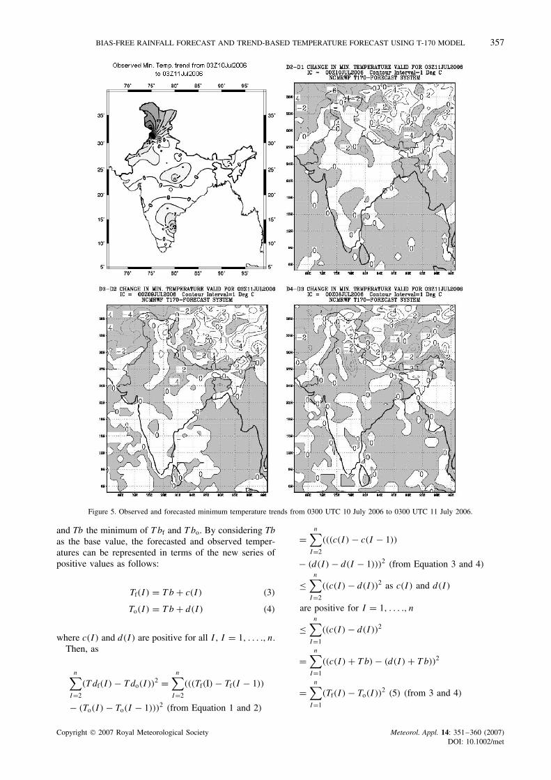
Figure 5. Observed and forecasted minimum temperature trends from 0300 UTC 10 July 2006 to 0300 UTC 11 July 2006.

and Tb the minimum of T bf and T bo. By considering Tbas the base value, the forecasted and observed temper-atures can be represented in terms of the new series ofpositive values as follows:

Tf(I ) = T b + c(I ) (3)

To(I ) = T b + d(I) (4)

where c(I ) and d(I) are positive for all I , I = 1, . . . ., n.Then, as

n∑

I=2

(T df(I ) − T do(I ))2 =n∑

I=2

(((Tf(I) − Tf(I − 1))

− (To(I ) − To(I − 1)))2 (from Equation 1 and 2)

=n∑

I=2

(((c(I ) − c(I − 1))

− (d(I ) − d(I − 1)))2 (from Equation 3 and 4)

≤n∑

I=2

((c(I ) − d(I))2 as c(I ) and d(I)

are positive for I = 1, . . . ., n

≤n∑

I=1

((c(I ) − d(I))2

=n∑

I=1

((c(I ) + T b) − (d(I ) + T b))2

=n∑

I=1

(Tf(I ) − To(I ))2 (5) (from 3 and 4)



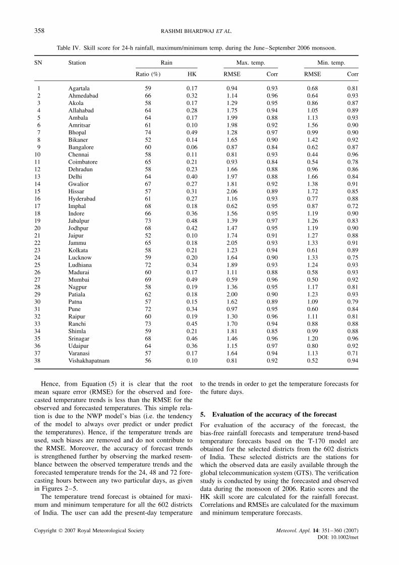
Table IV. Skill score for 24-h rainfall, maximum/minimum temp. during the June–September 2006 monsoon.

SN Station Rain Max. temp. Min. temp.

Ratio (%) HK RMSE Corr RMSE Corr

1 Agartala 59 0.17 0.94 0.93 0.68 0.812 Ahmedabad 66 0.32 1.14 0.96 0.64 0.933 Akola 58 0.17 1.29 0.95 0.86 0.874 Allahabad 64 0.28 1.75 0.94 1.05 0.895 Ambala 64 0.17 1.99 0.88 1.13 0.936 Amritsar 61 0.10 1.98 0.92 1.56 0.907 Bhopal 74 0.49 1.28 0.97 0.99 0.908 Bikaner 52 0.14 1.65 0.90 1.42 0.929 Bangalore 60 0.06 0.87 0.84 0.62 0.87

10 Chennai 58 0.11 0.81 0.93 0.44 0.9611 Coimbatore 65 0.21 0.93 0.84 0.54 0.7812 Dehradun 58 0.23 1.66 0.88 0.96 0.8613 Delhi 64 0.40 1.97 0.88 1.66 0.8414 Gwalior 67 0.27 1.81 0.92 1.38 0.9115 Hissar 57 0.31 2.06 0.89 1.72 0.8516 Hyderabad 61 0.27 1.16 0.93 0.77 0.8817 Imphal 68 0.18 0.62 0.95 0.87 0.7218 Indore 66 0.36 1.56 0.95 1.19 0.9019 Jabalpur 73 0.48 1.39 0.97 1.26 0.8320 Jodhpur 68 0.42 1.47 0.95 1.19 0.9021 Jaipur 52 0.10 1.74 0.91 1.27 0.8822 Jammu 65 0.18 2.05 0.93 1.33 0.9123 Kolkata 58 0.21 1.23 0.94 0.61 0.8924 Lucknow 59 0.20 1.64 0.90 1.33 0.7525 Ludhiana 72 0.34 1.89 0.93 1.24 0.9326 Madurai 60 0.17 1.11 0.88 0.58 0.9327 Mumbai 69 0.49 0.59 0.96 0.50 0.9228 Nagpur 58 0.19 1.36 0.95 1.17 0.8129 Patiala 62 0.18 2.00 0.90 1.23 0.9330 Patna 57 0.15 1.62 0.89 1.09 0.7931 Pune 72 0.34 0.97 0.95 0.60 0.8432 Raipur 60 0.19 1.30 0.96 1.11 0.8133 Ranchi 73 0.45 1.70 0.94 0.88 0.8834 Shimla 59 0.21 1.81 0.85 0.99 0.8835 Srinagar 68 0.46 1.46 0.96 1.20 0.9636 Udaipur 64 0.36 1.15 0.97 0.80 0.9237 Varanasi 57 0.17 1.64 0.94 1.13 0.7138 Vishakhapatnam 56 0.10 0.81 0.92 0.52 0.94

Hence, from Equation (5) it is clear that the rootmean square error (RMSE) for the observed and fore-casted temperature trends is less than the RMSE for theobserved and forecasted temperatures. This simple rela-tion is due to the NWP model’s bias (i.e. the tendencyof the model to always over predict or under predictthe temperatures). Hence, if the temperature trends areused, such biases are removed and do not contribute tothe RMSE. Moreover, the accuracy of forecast trendsis strengthened further by observing the marked resem-blance between the observed temperature trends and theforecasted temperature trends for the 24, 48 and 72 fore-casting hours between any two particular days, as givenin Figures 2–5.

The temperature trend forecast is obtained for maxi-mum and minimum temperature for all the 602 districtsof India. The user can add the present-day temperature

to the trends in order to get the temperature forecasts forthe future days.

5. Evaluation of the accuracy of the forecast

For evaluation of the accuracy of the forecast, thebias-free rainfall forecasts and temperature trend-basedtemperature forecasts based on the T-170 model areobtained for the selected districts from the 602 districtsof India. These selected districts are the stations forwhich the observed data are easily available through theglobal telecommunication system (GTS). The verificationstudy is conducted by using the forecasted and observeddata during the monsoon of 2006. Ratio scores and theHK skill score are calculated for the rainfall forecast.Correlations and RMSEs are calculated for the maximumand minimum temperature forecasts.



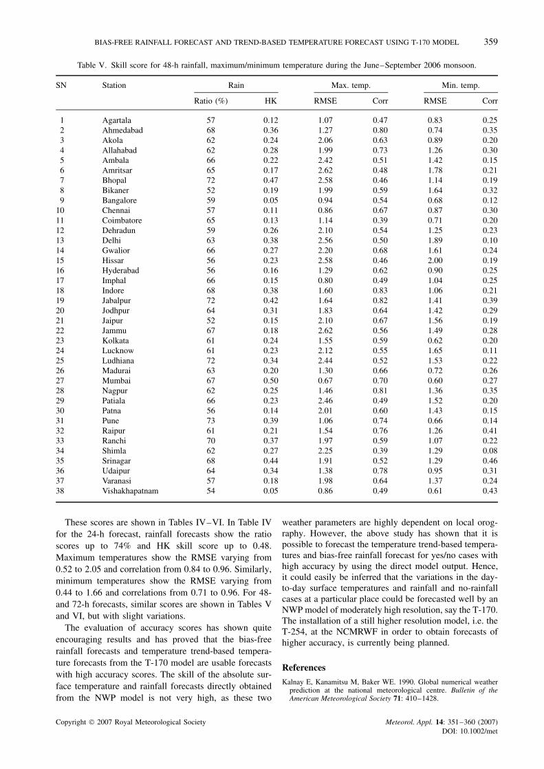
Table V. Skill score for 48-h rainfall, maximum/minimum temperature during the June–September 2006 monsoon.





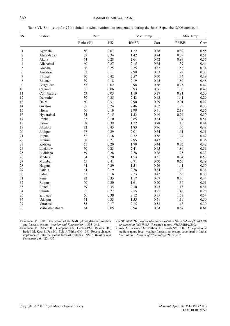
These scores are shown in Tables IV–VI. In Table IVfor the 24-h forecast, rainfall forecasts show the ratioscores up to 74% and HK skill score up to 0.48.Maximum temperatures show the RMSE varying from0.52 to 2.05 and correlation from 0.84 to 0.96. Similarly,minimum temperatures show the RMSE varying from0.44 to 1.66 and correlations from 0.71 to 0.96. For 48-and 72-h forecasts, similar scores are shown in Tables Vand VI, but with slight variations.

The evaluation of accuracy scores has shown quiteencouraging results and has proved that the bias-freerainfall forecasts and temperature trend-based tempera-ture forecasts from the T-170 model are usable forecastswith high accuracy scores. The skill of the absolute sur-face temperature and rainfall forecasts directly obtainedfrom the NWP model is not very high, as these two

weather parameters are highly dependent on local orog-raphy. However, the above study has shown that it ispossible to forecast the temperature trend-based tempera-tures and bias-free rainfall forecast for yes/no cases withhigh accuracy by using the direct model output. Hence,it could easily be inferred that the variations in the day-to-day surface temperatures and rainfall and no-rainfallcases at a particular place could be forecasted well by anNWP model of moderately high resolution, say the T-170.The installation of a still higher resolution model, i.e. theT-254, at the NCMRWF in order to obtain forecasts ofhigher accuracy, is currently being planned.

References

Kalnay E, Kanamitsu M, Baker WE. 1990. Global numerical weatherprediction at the national meteorological centre. Bulletin of theAmerican Meteorological Society 71: 410–1428.



Table VI. Skill score for 72-h rainfall, maximum/minimum temperature during the June–September 2006 monsoon.





Kanamitsu M. 1989. Description of the NMC global data assimilationand forecast system. Weather and Forecasting 4: 335–342.

Kanamitsu M, Alpert JC, Campana KA, Caplan PM, Deaven DG,Iredell M, Katz B, Pan HL, Sela J, White GH. 1991. Recent changesimplemented into the global forecast system at NMC. Weather andForecasting 6: 425–435.

Kar SC 2002. Description of a high-resolution Global Model(T170/L28)developed at NCMRWF , Research report, NMRF/RR/1/2002.

Kumar A, Parvinder M, Rathore LS, Singh SV. 2000. An operationalmedium range local weather forecasting system developed in India.International Journal of Climatology 20: 73–87.


bias-free rainfall forecast and temperature trend-based ...eder/artigos/bias/bhardwaj_2007.pdf ·...

Documents