bethesda, md 20084-5000 ad-a272 187 i 11111111111111 ml ... realistic for propulsors operating in an...

Carderock Division, Naval Surface Warfare CenterBethesda, MD 20084-5000

AD-A272 187I ml 11111111111111 !111tll 1111

CRDKNSWC/HD-1262-06 October 1993

Hydromechanics DirectorateResearch and Development Report

Reynolds-Averaged Navier-StokesCodes and Marine PropulsorAnalysis

byDaniel T. Valentine

(0

0tmt

CU,

(0

0)"M0

0/ ..... -- -- !I

""P II

CL0

(L

t--

zC

C •Approved for public release; distribution is unlimited.M0

CODE 011 DIRECTOR OF TECHNOLOGY. PLANS AND ASSESSMENT

12 SHIP SYSTEMS INTEGRATION DEPARTMENT

14 SHIP ELECTROMAGNETIC SIGNATURES DEPARTMENT

15 SHIP HYDROMECHANICS DEPARTMENT

16 AVIATION DEPARTMENT

17 SHIP STRUCTURES AND PROTECTION DEPARTMENT

18 COMPUTATION, MATHEMATICS & LOGISTICS DEPARTMENT

19 SHIP ACOUSTICS DEPARTMENT

27 PROPULSION AND AUXILIARY SYSTEMS DEPARTMENT

28 SHIP MATERIALS ENGINEERING DEPARTMENT

DTRC ISSUES THREE TYPES OF REPORTS:

1. DTRC reports, a formal series, contain information of permanent technical value.They carry a consecutive numencal identification regardless of their classification or theoriginating department.

2. Depwrtmenftl reports, a semiformal series, contain information of a preliminary,temporary, or proprietary nature or of limited interest or significance. They carry adepartmental alphanumerical identification.

3. Technical memoranda, an informal series, contain technical documentation oflimited use and interest. They are primarily working papers intended for internal use. Theycarry an identifying number which indicates their type and the numerical code of theoriginating department. Any distribution outside DTRC must be approved by the head ofthe originating department on a case-by-case basis.

UNCLASSIFIEDSECURITY CLASSIiCATION OF THIS PAGE

REPORT DOCUMENTATION PAGEIa. REPORT SECURITY CLASSIFICATION lb. RESTRICTIVE MARKINGS

UNCLASSIFIED2a. SECURITY CLASSIFICATION AUTHORITY 3 DISTRIBUTIONIAVAILABILITY OF REPORT

2b. DECLASSIFICATIONIDOWNGRADING SCHEDULE Approved for public release; distribution is unlimited.

4. PERFORMING ORGANIZATION REPORT NUMBER(S) 5. MONITORING ORGANIZATION REPORT NUMBER(S)

CRDKNSWCIHD-1262-06

6A. NAME OF PERFORMING ORGANIZATION 6b. OFFICE SYMBOL 7a. NAME OF MONITORING ORGANIZATION

Carderock Division (I1 applicable)

Naval Surface Warfare Center Code 544

6c. ADDRESS (City, State, and ZIP Code) 7b. ADDRESS (CITY, STATE, AND ZIP CODE)

Bethesda, MD 20084-5000

Sa. NAME OF FUNDING/SPONSORING 6b. OFFICE SYMBOL 9. PROCUREMENT INSTRUMENT IDENTIFICATION NUMBERORGANIZATION (I1 applicable)

Office of Chief of Naval Research Code 45248c. ADDRESS (City, State, and ZIP code) 10. SOURCE OF FUNDING NUMBERS

PROGRAM PROJECT TASK WORK UNITELEMENT NO. NO. NO ACCESSION NO

800 N. Quincy St., Arlington, VA 22217-5000 NO. RCCECIO D O0602121 N RH21C14 DN501142

11. TITLE (Include Security Classification)

Reynolds-Averaged Navier-Stokes Codes and Marine Propulsor Analysis

12. PERSONAL AUTHOR(S) Daniel T. Valentine

13a. TYPE OF REPORT 13b. TIME COVERED 14. DATE OF REPORT (Year, Month, Day) 15. PAGE COUNTFin FROM To 1993 October

16. SUPPLEMENTARY NOTATION

17. COSATI CODES 18. SUBJECT TERMS (Continue on Reverse It Necessary and identity by Block Number)FIELD GROUP SUB-GROUP Viscous Flow Hydrodynamics

Propeller PANSPropulsor DTNS

19. ABSTRACT (Continue on reverse it necessary and identity by block number)

This report describes the application of Reynolds-Averaged Navier-Stokes (RANS) codes to viscous-flow problems associated with marinepropulsors. The theory behind RANS codes is described, and the numerical solution methods typically applied to solve the RANSequations are discussed. A description of the strengths and limitations of applying RANS codes to predict real fluid effects is given.Careful scrutiny and engineering judgment must be exercised in the interpretation of predictions based on the turbulence models typicallyembodied in RANS codes. Two benchmark computations using DTNS3D, a typical RANS code, are presented to illustrate interpretationconcerns. The examples include flow over a pipe expansion and flow over the leading edge of a blunt reLangular plate.

20 DISTRIBUTION/AVAiLABILITY OF ABSTRACT 21. ABSTRACT SECURITY CLASSIFICATION0 UNCLASSIFIED/UNLIMITED 10 SAME AS RPT, 0 DTIC USERS UNCLASSIFIED

22a. NAME OF RESPONSIBLE INDIVIDUAL 22b. TELEPHONE (Include Area Code) 22c. OFFICE SYMBOLFrank B. Peterson (301) 227-1450 Code 1544

DD FORM 1473,84 MAR UNCLASSIFIEDSECURITY CLASSIFICATION C- TI;3 PAGE

ii CRDKNSWC/HD-1 262-06

CONTENTS

PageA bstract .............................................................................................................................. 1

A dm inistrative Inform ation ............................................................................................. I

Introduction ....................................................................................................................... I

T heory ................................................................................................................................ 2

Turbulence M odeling ....................................................................................................... 5

Tw o-Equation, k - e M odel ........................................................................................... 9

Baldw in-Lom ax A lgebraic M odel ................................................................................. . 11

Com putational M ethods .................................................................................................. 13

Derivation of FD M ....................................................................................................... 14

Tw o-D im ensional Com putational M ethods .................................................................. 22

RA N S C odes ...................................................................................................................... 25

Propulsor M odeling ......................................................................................................... 27

Sum m ary ........................................................................................................................... 30

A cknow ledgm ents ............................................................................................................ 32

References .......................................................................................................................... 33

FIGURES

1. Illustration of the boundary-value problem of a body in a uniform stream .............. 5

2. Illustration of an elemental control vlume for two-dimensional problems ................ 15

Y, 3. O ne-dim ensional finite-difference grid structure ...................................................... 17

4. Two-dim ensional finite-difference grid structure ...................................................... 24

CRDKNSWC/HD-1 262-06

V ~CRDKNSWC/HD-1 262-06

ABSTRACT

This report describes the application of Reynolds-Averaged Navier-Stokes (RANS) codesto viscous-flow problems associated with marine propulsors. The theory behind RANS codes isdescribed, and the numerical solution methods typically applied to solve the RANS equations arediscussed. A description of the strengths and limitations of applying RANS codes to predict realfluid effects is given. Careful scrutiny and engineering judgment must be exercised in theinterpretation of predictions based on the turbulence models typically embodied in RANS codes.Two benchmark computations using DTNS3D, a typical RANS code, are presented to illustrateinterpretation concerns. The examples include flow over a pipe expansion and flow over theleading edge of a blunt rectangular plate.

ADMINISTRATIVE INFORMATION

This report is submitted in partial fulfillment of the Milestone 4, Task I of the Advanced

Propulsion Systems Project (RH21 C14) of the FY93 Surface Ship Technology Block Plan

(NDIA/P30602121N). The work described herein was sponsored by the Office of the Chief of

Naval Research (ONR 4524) and performed at the David Taylor Model Basin, Headquarters,

Carderock Division, Naval Surface Warfare Center, by the Hydromechanics Directorate,

Propulsor Technology Branch (Code 544), and was funded under DN501142, Work Unit

1506-352.

INTRODUCTION

In the design of fluids engineering devices that use slender bodies and lifting surfaces as

their components, the application of potential flow methods are useful. This fact is particularly

true in the design and performance evaluation of marine propulsors. In the analysis of slender

bodies or lifting surfaces viscous effects are assumed to be confined to thin boundary-layers

adjacent to the solid surfaces of the body that moves (or is propelled) through a fluid. The flow

field exterior of the boundary-layers is assumed to be potential. These assumptions are known to

be realistic for propulsors operating in an irrotational free-stream (or onset flow). In many design

scenarios, however, the propulsor operates in the wake of the ship it is designed to propel. In

these situations the inflow is rotational, i.e., it has finite vorticity or internal shear stresses. When

the propulsor is designed to operate in a sheared onset flow it is still a reasonable approximation

to assume that the propulsor is a potential flow producer. In this case the effects of the propulsor's

induced flow on the distortion of the inflow vorticity must be taken into account. It is taken into

CRDKNSWC/HD-1 262--06 1

account by computing an effective inflow either empirically or by applying a computational

method that computes the additional induced velocities associated with the stretching and turning

of the vorticity in the onset flow when it is acted upon by the propulsor. In conventional

propulsor-design practice, this distorted onset flow is called the effective wake. The wealth of

successful experience in the design of wake adapted propellers provides substantial support for

these assumptions.

Why would we need Reynolds-Averaged Navier-Stokes (RANS) codes in the analysis of

marine propulsor designs? In the conventional procedure for the design of ship hulls, the hull

shape is selected without regard to the detailed geometric configuration of the propulsor. The hull

is selected based on low tow resistance; hence, a nonseparating bare hull is typically designed. If

hulls with fuller stem shapes are desirable, then the potential for suppressing flow separation with

the propulsor cannot be ignored. In order to examine the propensity for a full stern hull to cause

flow separation and to examine the effect of propulsor design on suppressing flow separatioin, a

RANS code should be considered. This is because flow separation is primarily a real (or viscous)

flow effect. Additional opportunities for RANS analysis occur on the complex surfaces of

propulsor components.

This report presumes that there is an interest in applying a Navier-Stokes or (real fluid)

viscous flow code to evaluate a given propulsor design. In addition, it also presumes that time-

averaged flow properties are required. From a practical point of view a RANS code should

provide reasonable approximations of the time-averaged flow properties in high Reynolds

number flows around complex geometries.

What is involved in selecting and using a RANS code? It is this question that is

considered in this report. The theory of turbulence modeling typically implemented in RANS

codes is described. This description is followed by a description of the computational methods

required to solve the RANS equations. The selection of grids and other issues related to the

application of a RANS code are discussed. Finally, two RANS codes that could be used by the

marine propulsor designer are described.

In the next section of this report the theory that describes the flow of water is presented.

This theory is the foundation on which the models to predict the time-averaged flow properties of

a turbulent flow are built.

2 CRDKNSWC/HD-1262-06

THEORY

It is well known in the fluid mechanics community that the Navier-Stokes equations are

the equations that model the dynamics of water and air (at low Mach number, less than 0.3). The

Navier-Stokes (N-S) and continuity equations in nondimensional form are as follows:

d + u I Vu = -VP + V2u, (1)dt

and

V U =0.

(2)The parameter 91 = UL/v is the Reynolds number, where U is the characteristic velocity of the

flow problem, e.g., the uniform speed of a ship, L is the characteristic length of the flow problem,

e.g., the overall length of a ship, and v is the kinematic viscosity of the fluid, e.g., for fresh water

v= 1.0 X 1-e m2s- at 200 C. Equations (1) and (2) are a set of four equations in four

unknowns, viz, the three components of the velocity vector u = (u,vw) and the dynamic pressureP = p/(pLU2). The density and kinematic viscosity are assumed to be constant. These are

reasonable assumptions for the flow of water at relatively high Reynolds numbers. Typical valuesof the Reynolds number in flows of practical interest are within the range 1 W"< 9? < Io".

The inverse of .9? is the coefficient of the viscous term in the N-S equations; it is

obviously small as compared to the coefficients of the other terms. The importance of viscosity in

high Reynolds number flows is evident for two reasons. The first reason is the physically realistic

no-slip boundary condition that must be imposed at the solid boundaries adjacent to the fluid.

This boundary condition causes large gradients in the mean velocity distribution near the

boundaries; hence, viscous boundary-layers are formed near the solid boundaries. The second

reason is the fact that the flow induced by the relative motion of a solid boundary with a viscous

fluid is highly unsteady (i.e., turbulent) in the high Reynolds number flows of practical interest.

The no-slip condition and turbulence are viscous flow phenomena; without the viscous terms inthe N-S equations these phenomena do not exist.

The no-slip boundary condition completes the mathematical statement of the flow

problem of a body moving through an incompressible fluid of infinite extent. Let us consider the

flow field induced by a body moving at constant speed through an incompressible fluid. From the

CRDKNSWC/HD-1262-06 3

viewpoint of a reference frame attached to the body, we observe a stationary body in a uniform

stream LA; see Fig. 1. The boundary condition on S8 may be written as follows:

u= 0 on S8 . (3)

This condition states that both the normal and tangential velocity components at the solid

boundary are equal to zero in the body fixed frame.

Equations (1) and (2) with the no-slip condition, (3), completely describe the flow

induced by a moving body, S8 , in an incompressible, viscous fluid of infinite extent. However.

for high 9? flows around arbitrarily shaped bodies this set of equations is intractable even by

computational methods with present day digital computers. This fact has led the engineering

community to seek other methods to predict the time-averaged flow properties in flows of

practical interest. Two of the more well known models for high Reynolds number turbulent flows

are described in the next section.

TURBULENCE MODELING

Viscous flows at large values of .91 are in general unsteady (i.e., turbulent). The design

conditions for most hydrodynamic devices are imposed at a steady characteristic speed, e.g., at a

prescribed ship speed or onset flow. Therefore, a computational analysis method is desirable that

allows the engineer to obtain approximate solutions foi ,he time averaged flow properties in high

Reynolds number turbulent flows.

Reynolds, in 1895, proposed the following decomposition of the flow properties. lie

assumed that the velocity field can be decomposed into a mean, U, and a random fluctuation, u',

such that

U = f + U', (4)

where

Ui 1 urn.- f+TT u dt,TT,- "TT r,,

u- lir f T r(u -ii)dt = 0


- - Sb

MO/

U"---____ -___--_

Fig. 1. Illustration of the boundary-value problem of a body in a uniform stream.

CRDKNSWC/HD-1 262--06 5

Similarly,

p= P + P'. (5)

Substituting (4) and (5) into (1) and (2) and taking the time average (as defined above) of

the resulting equations, we obtain the Reynolds-Averaged N-S (RANS) equations, viz:

u - du, OP I d2u:.1 /()-+u - + (6)dt 1 dx, dx, .91 dx, dx, 9x

where, of course, du, / di = 0; however, the time derivative is included for two reasons. The

first reason is that artificial time-stepping is used as the iteration procedure for solving steady-

state problems in many of the available RANS codes. The second reason is to provide the option

of considering slowly varying unsteady flows, i.e., U = ii(x, t), in which the time scales of the

solid boundary oscillations are signific'ntly longer than the time scales, TT, of the turbulence

velocity fluctuations. In this report it is for the first reason that the time derivatives are retained.

(Note that Equation (6) is in component form in which Cartesian tens( r notation with Einstein's

summation convention is used. The velocity components implied by thi:., equation are u, = u, v

and w for i = 1, 2, and 3, respectively.)

From Equation (6) we set that a total stress tensor acting on the flow mnay be written in

the following, nondimensional form:

1 aY, aJ,T' .P6Qf+ + Ulu; .

The lattcr term is known as the Reynolds stress. Hencc, the only effect of the random velocity

fluctuations on the time averaged flow properties is the contribution of an additional stress

system.

The time averaged form of the continuity equation is:

du, =0 (7)

dx,


Equations (6) and (7) are a set of equations for the mean flow properties u, = u, v, or = 12

or 3, respectively, and P. However, the quantities uiu• are additional unknowns that arise from

the application of Reynolds decomposition. The faz: that the components of the Reynolds stress

tensor are additional unknowns is an illustration of the well known closure problem of turbulence.

The decomposition of the flow into a mean flow and turbulent velocity fluctuations

isolates the effects of the turbulent fluctuations on the mean flow. However, as pointed out above

and discussed in detail by Tennekes and Lumley (1974), there are additional unknowns that must

be determined. If we sought to derive additional equations for the components of the Reynoldsstress tensor from the original N-S equations, additional unknowns of the form u'u'u; are

generated by the nonlinear inertia terms. According to Tennekes and Lumley, this problem is

characteristic of all nonlinear stochastic systems. This is the closure problem; the system of

equations describing the mean flow cannot be closed without additional assumptions even though

the N-S equations and the continuity equation form a complete mathematical statement of the

actual time-dependent flow problem.

To attempt to solve the closure problem many engineering investigators have judiciously

guessed in attempts to find a relationship between

uuand I d x)+

These attempts are by analogy (in some sense) with the constitutive relationship for a Newtonian

fluid, viz:

= p + v (diu, o+du'p1]2 pu2 UL ~dx1 x

The equation for o+,, which is the stress tensor for a Newtonian fluid in component form, is a

phenomenological law which states that the stress at a point is the sum of the normal stress due to

pressure plus the viscous stress, which is linearly dependent on the rates of strain (deformation) of

the fluid. This equation for q, is the constitutive equation used to derive the N-S equations from

the transport theorem; see for example Newman (1977). It is this equation that connects the

microscopic behavior of a liquid to its macroscopic behavior. (it is a well known fact that this

equation describes the behavior of water; see Truesdell, 1974.)

CRDKNSWC/HD-1 262-06 7

One of the most popular models that arises from judicious guessing is the 'standard' k - f-

model originally proposed by Launder and Spalding (1974). The 'standard' model, which is the

model presented below, is not very general. It must be extended to include the effects of

curvature, low Reynolds number, near wall, etc. Some of the extensions examined in the literature

to handle complex flow fields are discussed by Nallasamy (1987) among others. The ",(andard'

model mainly applies to nearly parallel, high Reynolds number flows. The 'standard' k - e model

is called a two-equation turbulence model since two additional differential equations must be

solved along with Equations (3) and (4). Because it does not handle near-wall flows, a wall-

function model is required to satisfy the no-slip boundary condition at solid walls. The 'standard'

k - E model with the wall-function boundary condition works adequately as long as the

assumptions inherent in the model are not greatly violated; numerous successful applications of

this model in studies of a wide variety of flow problems have been reported in the literature. The

mathematical statement of this two-equation turbulence model is given in the next subsection.

The algebraic turbulence model reported by Baldwin and Lomax (1978) is an alternative

model. It is simpler than the two-equation model already described and, for high .9i' flows, has a

wider range of applicability. Models of this type have found successful application in the

prediction of separated flows; see for example Gee, Cummings and Schiff (1990). These models

work well in flows where viscous effects are confined to boundary-lay,!rs and the external flow is

primarily inviscid in nature with or without finite vorticity. The problems of marine

hydrodynamics are generally of this type. The mathematical statement of this model is given in a

subsequent subsection.

The selection and application of a turbulence model is indeed an art. Once an appropriate

model has been selected, a computational method must also be selected to solve the model

equations. The selection and application of a computational method also requires judgment. The

issues that arise in the selection and implementation of a computational method to solve the

RANS equations will be discussed in a subsequent section of this report.

Note that the turbulence models to be presented next are to a great extent ad hoc. They

are tractable models that provide a means to estimate the time averaged flow fields of high

Reynolds number turbulent flows. They are not models of the complete physics of flow as are

Equations (1) and (2). The models are simplifications that attempt to provide the engineer with a

set of model equations that can be solved with todays computational technology. Considering the

successful experience with careful applications of turbulence models reported in the literature,

RANS codes should find successful application in the evaluation of flows of engineering interest

and, in particular, in the evaluation of some of the flow problems that arise in the design of


advanced marine propulsors. The experience to date, that has been reported in the engineering

literature, supports this contention.

TWO-EQUATION, k - E MODEL

The two equation model originally proposed by Launder and Spalding (1974) may be

derived from a rational mechanics viewpoint that includes considerations of the energy equation

and the second-law of thermodynamics; see Tannous, Ahmadi and Valentine (1989) and

Tannous, Valentine and Ahmadi (1990). It is a "phenomenological" model that assumes an eddy

viscosity analogous to the kinematic viscosity, i.e., it assumes

- VT ( +d_., ULI d~jdX)

If we define an effective viscosity as follows,

V =V+ VT

and note that vris not a constant, we may rewrite Equation (6), i.e., the RANS equations, as

follows:

du, - du dP +d I (dir u).+U _ I- -+ -d , (8)dt dx, dix, dx, - dx,)]

where

UL

V,

In this system of equations the effective viscosity is an unknown because VT is an unknown: thus,

the effective Reynolds number, .91,, is an unknown.

In two-equation turbulence models the Prandtl-Koimogorov hypothesis is usually

invoked. It relates the turbulent viscosity, VT, to the turbulent kinetic energy,k = 4uL'u,' and the

turbulent dissipation function, E. The Prandtl-Kolmogorov expression is, in dimensionless form,

as follows:


I = - = k 2

N UL

In order to close the system of equations we need equations for k and E.

The transport equations for the turbulent kinetic energy, k, and the turbulent dissipation

function, E, were originally reported by Launder and Spalding (1974). They are, in dimensionless

form:

dk -dk d [((Ck-1 1 + Ak _

dt 'dx, dx, [ C km k )dxJ(9)

dx dx, dx,U

and

-E +u- = (a , -1 1 +._.._ C.-E

dt dx, dx, [kg, 'g? ukdx,j k(1o)

)M k ~dx, dx, ) dx,

where the constants are as follows:

C' = 0.09, C" = 1.45, C'2 " 1.90, ok = 1.0, a, = 1.5.

These constants are not meant to be changed; they are assumed to be universal. This completes

the mathematical statement of the flow field equations for the 'standard' k - E model. Equations

(7), (8), (9) and (10) are a set of 6 equations in 6 unknowns, viz, the three components of velocity,

(u, v, w,) the pressure, P, the turbulent kinetic energy, k, and the turbulence dissipation, c.

Since near-wall flows are not appropriately modeled with this formulation, a wall-

function boundary condition or other near-wall treatment must be applied. In the near-wall region

the boundary conditions may be imposed in the logarithmic layer of the near-wall boundary layer

10 CRDKNSWC/HD-1 262-06

by invoking the universal law-of-the-wall. Using this logarithmic law and the assumption of local

equilibrium, equations that provide the necessary boundary values for k and E have been

developed. Modifications to this approach have also been reported in the literature to extend the

near-wall model in conjunction with exttending the k - E model to handle complex flows.

If the two-equation model just described does not predict a particular flow field correctly,

then the flow field most likely violates the assumptions made in the derivation of the model.

Again, we must keep in mind that this model is not expected to work in highly curved flows, in

near wall flows among other complex flows. There are a wealth of proposed modifications that

are reported in the engineering literature from which to choose an appropriate modification of this

two-equation model when it is required. It is up to the user to select the appropriate turbulence

model.

BALDWIN-LOMAX ALGEBRAIC MODEL

The Baldwin-Lomax model has been used extensively since its introduction because of

its computational efficiency and accuracy; see Baldwin and Lomax (1978). This model was

patterned after the model developed by Cebeci et al (1977). This and four similar models were

applied and compared by Gee et al (1990) to investigate the flow about a prolate spheroid at high

angle of attack. For bodies that are at high angles of attack (27 to 30 degrees) the Baldwin-Lomax

model requires modification. For flows of practical interest to the marine hydrodynamicist at or

near design points in which flow separation is not expected to occur, this model is useful. In fact,

the recent experience of C.I. Yang (1991)1 with this model on problems of interest to the marine

propulsor designer is encouraging. The turbulence model equations for the Baldwin-Lomax

formulation are presented next.

This model is also an eddy viscosity model that assumes an effective kinematic viscosity,

i.e.,

V, = V + VT.

The turbulent flow is assumed to be divided into an inner and outer region with a different set of

equations used in each region to determine the turbulent eddy viscosity, v7. The value of v, is

defined as follows:

I Pcrsonal communication.

CRDKNSWC/HD--1262-06 11

., = mi [( VT)InneV) . (11)

In the inner region the Prandtl-Van Driest formulation is used to determine VT This formula is

(VT)., = 12Q,

where

= ky [1.0 e-(y/A')

y. ,...y- (rjp)½y

V. V.

and

Q= du d +( dv dw I + du

dy -dx + "-dz * • dx dz '

the latter of which is the magnitude of the local vorticity.

In the outer region, for attached boundary-layers, the turbulent viscosity is given by

(VT)r)u,,, = KC Fý.kFh,,y)

where

Fc = min [(y,..rF,..), (C..y ..... udif)],

in which udif is the difference between the maximum and minimum total velocity in the local

profile, i.e.,

Ud,1 C DNWD+W) V (0+W)


and

[']-jFKIa,(y) = 10+5.5 (C•Y)

F.,, is defined as the maximum value of the function,

F(y) = yQ1[LO-e-1Y'IA')]

for each streamwise location along the wall at y,,,, which is the normal distance from the surface

at which this maximum occurs.

The constants in the model (which are assumed to be universal) are as follows:

A+ =26, k = 0.4, CoF = 1.6,

K = 0.0168, CKCb = 0.3, C,, = 0.25.

This completes the mathematical statement of the Baldwin-Lomax algebraic turbulence model.

The model provides a method to compute the turbulent viscosity, vrand, hence,

1 v+ vr

UL

which is the only other unknown in the eddy viscosity version of the RANS equations. Hence,

Equations (7), (8) and (11) are a set of five equations in five unknowns, viz, the three components

of velocity, (u, v, w,) the pressure, P, and the eddy viscosity, VT.

COMPUTATIONAL METHODS

The boundary-value problems described in the previous section cannot in general be

solved by analytical methods. If we are interested in solving these equations we must resort to

approximate, computational methods that may be implemented on a digital computer. One class

of computer methods is finite difference methods. (There are several other well-known classes of

computational methods, viz., finite-element methods, spectral methods, and equivalent-vortex


methods.) A relatively large class of finite difference methods fall into the category of finite

volume, finite difference methods. The derivation of a finite volume scheme assumes that the

flow domain is discretized into small control volumes within which integral forms of the the

model equations are satisfied. The approximations associated with the application of

computational methods may be illustrated by a derivation of one-dimensional methods. Such a

derivation is presented to illustrate the assumptions required to develop a computational method.

A two-dimensional finite difference method is subsequently presented that is a

generalization of the one-dimensional method described. The two-dimensional method is

presented to illustrate the problems associated with going to higher dimensions.

DERIVATION OF FDM

The transport equations of the turbulence models, viz, Equations (6), (9) and (10), have

the following structure (in component form):

df + f = (D L-)I + S, (12)dt 3x dx kax)

or (in the Gibbs vector notation form):

df + uV = V.(DVf) + S, (13)

dt

wheref'= u, v, w, k, or e. Utilizing the continuity equation, V -u =, we may write (13) in the

following, so-called conservative or divergence form:

+ V-(uf) = V,(DVf) + S, (14)dt

To solve a differential equation of the form (14) we must, of course, integrate. This is done next

by a finite difference method.

Consider the elemental control volume illustrated in Fig. 2. This control volume is

assumed to be a discrete subdomain of the flow field of interest. Integrating Equation (14) over

this arbitrarily selected control volume, C. V., wz obtain:


77Elemental C.V.

... IA....

X.

Fig. 2. Illustration of an elemental control volume for two-dimensional problems.

CRDKNSWC/HD-.1 262-06 15

fffc -dV. = fff cv[-V.(uf)+V'(DVf)+S]dV. (15)

Equation (15) is the form of the transport equation from which the finite difference method is

derived.

Let us consider the one-dimensional problem illustrated in Fig.3. In this case we assume

that u = u i,f=j(x,t) and S = S(xt). In this case, after applying the theorem of Leibnitz, Equation

(15) reduces to

ffNf- .fdV = fff [td)f.i(D +)S1 dV, (16)

in which dV = dxdydz. Next, we integrate over unit distances in the y and z directions, and in the x

direction from x, - Ax/2 to xi + Ax/2. Integrating, we get

+d .- x+(uf)Rl - (L= . [d D 1x) +S dx. (17)

Finally, we may write Equation (17) as follows:

df _ (Uf)R - (uf + I [ D I + F(t), (18)dt Ax Ax k dx) k x), (1)

where f and S are the spatial averages off and S, respectively, over the control volume, C. V.

The functions fR,f.,, and their derivatives are the instantaneous values off and its derivative onthe right, R, and left, L, faces of the surface of the control volume. Integrating (14) from t to t+At,

we obtain

in+I - = F(t) dt, (19)

where the superscript n+1 identifies the value of the function at time t+At and the superscript n

identifies the value of the function at time t. The Euler-explicit or forward-time approximation to

this integral is


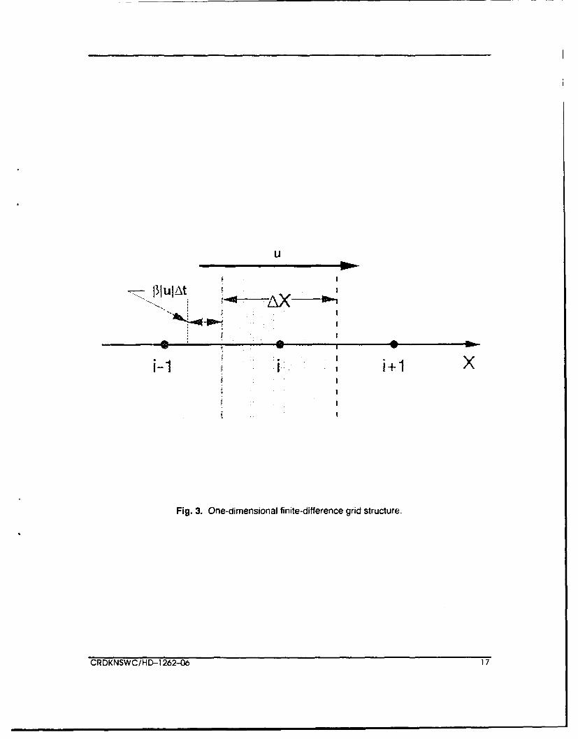
U

I3IuIAt -,-'- _ __

U At

* .41

i-1 1 I i+1 x

Fig. 3. One-dimensional finite-difference grid structure.


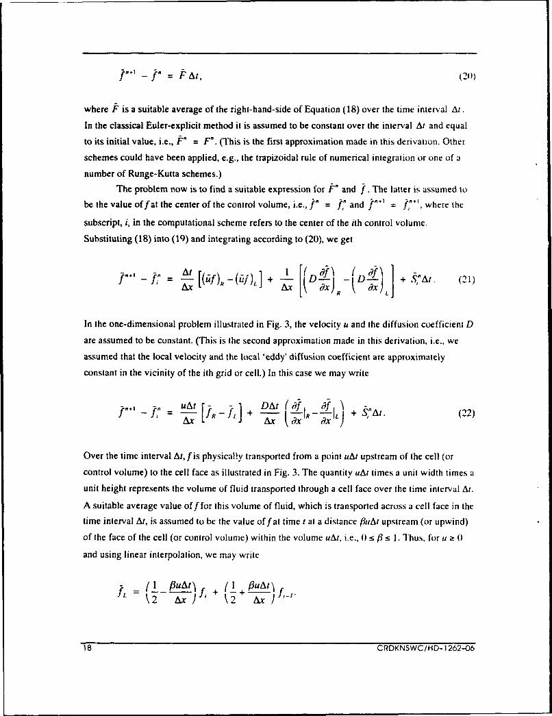
fi" - in = F At, (20)

where F is a suitable average of the right-hand-side of Equation (18) over the time interval At.

In the classical Euler-explicit method it is assumed to be constant over the interval At and equal

to its initial value, i.e., FPM = FP. (This is the first approximation made in this derivation. Other

schemes could have been applied, e.g., the trapizoidal rule of numerical integration or one of a

number of Runge-Kutta schemes.)

The problem now is to find a suitable expression for FT and f. The latter is assumed to

be the value of fat the center of the control volume, i.e., f n = f. and in*' = I,"', where the

subscript, i, in the computational scheme refers to the center of the ith control volume.

Substituting (18) into (19) and integrating according to (20), we get

At [W )M - (ff) I [(D1 d) (D~' 1 + SCAt. (21)Ax LJR XJL+ Ax ) ~dx) )LIJ

In the one-dimensional problem illustrated in Fig. 3, the velocity u and the diffusion coefficient D

are assumed to be constant. (This is the second approximation made in this derivation, i.e., we

assumed that the local velocity and the local 'eddy' diffusion coefficient are approximately

constant in the vicinity of the ith grid or cell.) In this case we may write

fP" - fi = -- [+ A X (iR- L) + $nAt. (22)

Over the time interval At, f is physically transported from a point uAt upstream of the cell (or

control volume) to the cell face as illustrated in Fig. 3. The quantity uAt times a unit width times a

unit height represents the volume of fluid transported through a cell face over the time interval A/.

A suitable average value off for this volume of fluid, which is transported across a cell face in the

time interval At, is assumed to be the value off at time t at a distance 3uAt upstream (or upwind)

of the face of the cell (or control volume) within the volume uAt, i.e., 0: r3 Ps 1. Thus, for u a( 0

and using linear interpolation, we may write

_t (1 fluAt ] (1 __ut_

( I _ PuAtj ,+(If utk 2 Ax ) k2 Ax ''


or- +PC)

(2L -PC . +(2

(This is the third approximation, i.e., a linear interpolation function was selected to estimate the

upwind value off.) Similarly,

fR= P~fc)f..+ 1 + (-+PiCf

Thus,

JR fL (2 ( PC) f,+ I + 2iC f, (2 (~+ PC) f1, (23)

Substituting Equation (23) into (22) and applying second-order central differences to the d/dx

terms in (22), we get the finitie difference analog of the transport equation, Equation (14), viz:

, = (1 - 23C2 - 2r) f" + (C2 +--+r) f-, + 2C4 - ) + r ,2 2 (24)

+ S,•,At,

where the choice of /3 distinguishes between various schemes. This class of Euler-explicit/3

schemes was in%. ligated by Valentine (1987,1988). The parameter C a uAt / Ax is the Courantnumber. The parameter r = DAt / (Ax) 2 = C / .91, is the Courant number divided by the cell

Reynolds number. The cell Reynolds number is .9?,A, uAx / D, where D is the local diffusion

or effective viscosity coefficient. The local Courant number and the local cell Reynolds number

play an important role in determining the stability of the computational method.

Equation (24), by virtue of the parameter f, contains a number of well known finite

difference schemes. If r = 0, C = 0, and S = 0, f2' = f'"', which means there is no motion

and no internal sources off. lfC -0 0, C2 << C, then for 3 = 0.5, this scheme -duces to the

forward-time centered-space difference scheme. Other relatively well known schemes that are

embodied in this equation are as follows. If P3 =1/(2C), then the advection (or convection) term

reduces to the second upwind (or donor-cell) advection scheme. If P = 1/2 and .qA, -* X, which

means r 0- , the scheme is the Lax-Wendroff scheme. If 3 = 1/2, for C = I the equation is pure

CRDKNSWC/HD-1262--06 19

upwind and exact for pure advection (no diffusion, i.e., r = 0, and no internal sources, i.e , S = 0).

If C - 0 the scheme approaches the second-order centered difference scheme. Finally, ifv. =

c./(2C), wht .e 0 < a < 1 is a weighting parameter, the scheme reduces to the weighted-upwind

scheme. The special cases cited above of the scheme given by Equation (24) are in the textbook

by Roache (1972) on computational fluid dynamics. Other variations of the Euler-explicit il

scheme are reported by Valentine (1988).

To examine the problems associated with selecting and implementing a computational

method it is instructive to study the mi)dified equation that corresponis to the difference equation,

Equation (24). If we nondimensionalize (24) in terms of the local characteristic scales, i.e.,

* = , =

A.- At

and let

S a - f,

we may write the modified equation for the scheme given by Equation (24) as follows:

9s+ -s d2s = C2 1) a~s +C r+ C-2- S

dt dx dx*2 2) 6 x"

+ C 2(25)

where the terms on the right-hand-side are the truncated terms (or truncation error) of the scheme

explicitly exposed. This equation is derived by substituting the Taylor series approximations of

the terms not in the center of the ith cell and not at time t in terms of the value of s and its

derivatives at time t and at the center of the ith cell, viz, in ierms ofs = s,". The truncation error

shows that Equation (24) is a first-order upwind scheme if /3 * 1/2; if /3 = 1/2, then the schcme is a

second-order scheme.

The second derivative truncation error produces numerical (or false) diffusion that is

analogous to physical diffusion. The third derivative truncation error produces wave-like behavior

or 'wiggles' in the solution near steep gradients, i.e., at Ications in the flow field whcre v changes

nearly discontinuously so that d's/ldx" is relatively large. This error is an error of inconsistency of


the difference scheme in that it actually approximates an equation with a third derivative term b\

virtue of the truncation error instead of the original differential equation for which the right-hand-

side of (25) is identically zero. Fine mesh or more grid points where gradients of s are large will

tend to suppress the wiggles because the third derivative of s will be reduced. It is reduced when

the mesh is refined because s is a continuous function. The modified equation was

nondimensionalized in terms of the grid size deliberately to illustrate this computational problem.

Hence, a fine mesh is required in regions of the flow where s is expected to have large gradients.

The selection of grid size, Ax, in conjunction with the selection of the time step, At

(which may be viewed as the selection of the iteration step for problems in which the steady

solution is sought), is not completely arbitrary. The Courant number is proportional to At/Ax and

the cell Reynolds number is proportiopnal to Ax; hence, they are measures of the time step and

the grid size. It can be shown from heuristic and von Neumann stability considerations that the

following restriction is imposed on the selection of these parameters:

C S (26)2(1 + 3C•?A,)

For the case in which M.a, -" cc, this restriction on C reduces to

C2 5 1- (27)

2P3

If/3 = 1/2, then Equation (27) reduces to the well known CFL (or Courant-Friedrichs-Lewy)

condition.

Within the framework of the last three equations, let us examine the effects of increasing

grid resolution. If Ax - small, then M., - small. Because C 5 .9 ?a,/2 (approximately) from

Equation (26), r - 1/2. Hence, for small grid size or high resolution of rapidly varying values of s

the local or cell Reynolds number is small which leads to a relatively large coefficient, r, of the

diffusion term and a relatively small value of C. This means that locally physical diffusion will

smooth the solution at the expense of smaller time steps (or iteration steps). Of course, this is not

unexpected; if more accuracy is required, then the computational effort required must increase.

For small values of Ax, the value of C is reduced and, hence At is reduced. This shows that a

greater number of equations over a greater number of time steps are required to reach a steady

solution.


There have been a number of successful extensions to the second-order scheme just

described that reduces the problems associated with the truncation error for relatively coarse

grids. The schemes go by the names flux-corrected transport (or FCT) and total variation

diminishing (or TVD) schemes. These refinements are designed to modify first- and second-order

schemes to suppress the problems that are associated with the second and third derivative

truncation errors particularly in the vicinity of step gradients of s. In the preliminary stages of a

computational investigation it may be useful to use the lower-order schemes with greater

numerical damping when the grid selection and debugging process is underway. If large gradients

in s are anticipated from the results of preliminary investigations and/or experience, then finer

grid structures in these regions along with the implementation of an FCT or TVD scheme wouldbe useful. For practical purposes, these refinements should be sufficient to handle most of the

practical problems confronted by the marine propulsor designer today. (in addition, before more

complex models and computational methods are used, experience with the set of tools described

in this report would be useful and, at least, an important first step in the implementation of CFD-

RANS codes in hydrodynamic design.)

TWO-DIMENSIONAL COMPUTATIONAL METHODS

Many two- and three-dimensional methods implement one-dimensional methods, that are

similar to the method just described, in each of the coordinate directions with the assumption that

the local flow field is nearly perpendicular to one of the grid faces. The experience reported in the

literature indicates that even if the flow is not necessarily perpendicular to one of the finite

difference cell faces the methods as constructed this way still provide reasonable approximations

of the solutions sought. The primary purpose of this section is to present a logical extension of the

one-dimensional method to illustrate the increase in complexity associated with coding

mutidimensional methods. The extension presented is the simplest two-dimensional method forwhich a rectangular mesh is assumed. As one can easily imagine, even without computational

fluid dynamics experience, the algebra invloved in deriving nonrectangular grid approximations

would indeed be more complex particularly if the same order accuracy is to be maintained.

Let us consider the two-dimensional flow problem illustrated in Fig. 2. The characteristic

length, L, and the characteristic velocity, U, are identified in the figure. The two-dimensional

version of the model transport equation for fis

Lf +duf +dwf =_ a D f) + d tD. +S.(28dt dx dz dxS dx) dx- dz)


The two-dimensional extension of Equation (24) as applied to (28) is as follows:

"'It= +](29)

+ [. , + ++ ' -+ f fn sT,

The finite difference cell for this formulation is illustrated in Fig. 4. The grid, for illustration

purposes, is assumed square, i.e., Ax = Az = h. The local diffusion coefficient is assumed to beconstant (or slowly varying locally). Note that D,'J is the local value of D. Three methods to

estimate f1R fL, fr, and fi are described next. They are identified by the numbers 1, 2 and 3 in

Fig. 5. They are called: (1) Second-upwind. (2) Skew-upwind. (3) Euler-explicit P3 scheme (with

/3 = 1/2). The parameterlul is the magnitude of the velocity vector in the direction of the arrow in

the figure. Case I is an extension of the donor-cell method to two-dimensional problems; it is

described in the book by Roache (1972). The proper extension of the one-dimensional donor-cell

method is Case 2, or the skewed-upwind scheme (as it has been called in the literature). It

requires, in addition to the same numerical operations in the x and z directions as Case 1, the

linear interpolation of f between the grid points (i - 1j) and (i - lj - 1) for the example illustrated

in the figure. The method of Case 3 requires bilinear interpolation between these points and

points (ij) and (ij - 1). Case 3 is the proper two-dimensional extension of the one-dimensional/3

scheme. The important point to note here is that the proper extensions require additional

computations; hence, they require more than a proportional increase in computational effort as

compared to their one-dimensional counterparts. The method typically used to extend one-

dimensional methods is analogous to Case 1. The modifications that improve the numerical

performance of the second-upwind scheme that goes by the names FCT and TVD are invariably

applied along the direction of the grid lines. Hence, there is an implicit assumption made by this

procedure, viz, the flow is in the direction of the vertical or horizontal grid lines. In fact,

nonuniform grid methods are usually designed with this assumption applied. This assumption is

important because it reduces the computational effort required; without this assumption thc

computational effort is indeed increased as was illustrated by Cases 2 and 3.

The stability criteria for multidimensional schemes are known to be more restrictive than

for one-dimensional schemes; see, for example, Hirt (1968) or Roache (1972). The fact that the

selection of grid size and time-step size is restricted by numerical stability considerations in

addition to accuracy requirements is important. If a selection is made that exceeds the stability


i-1 j+ ji i+1 j+

1 q pr' P

- -I

2. .. .. ... . .. .. ..

... .. ..

I I.. ...

Fi. . wodienioalfiit-dffrecegrd trctre

24 CRDKNSW./HD...2.2-0

bounds, the solution blows up rapidly; hence, precise knowledge of the stability bounds is not

particularly important. In addition, accuracy requirements tend to demand much finer meshes as

compared to the stability restrictions. Finally, the effects of the nonlinearities in the original

differential equation prevent an exact assessment of the stability bounds of the nonlinear

algebraic system of equations. Fortunately, the wealth of experience in applying a variety of

computational fluid dynamics methods to multidimensional problems that have been reported in

the literature illustrates that these issues are not the main problems in implementing

computational methods. The primary concerns are to ensure accuracy by comparing solutions to

known solutions, comparing solutions with solutions found using different methods and

comparing solutions with experimental data. The principal objectives of a computational study

are: (1) to demonstrate that the computational method produces reansonable approximations of

the model equations; (2) to demonstrate that the turbulence model is the appropriate model for the

kind of flow problem to be solved; (3) to provide a computational solution of the problem posed

to help make engineering decisions about hydrodynamic devices.

We cannot expect that all fluids engineers with a need for turbulent flow approximations

be experts in the development and implementation of computational turbulence models.

However, we can expect the fluids engineer, because of his or her academic background, to use

existing tools successfully. The application of the relatively crude RANS tools by the engineering

community has and will continue to help the research community in their quest to modify the

methods to more suitably handle particular classes of flows. In the area of the design of marine

propulsors there is a need to determine the usefulness of existing turbulence models. What

computational tools or computer programs are available to the marine propulsor engineer? I his

question is considered in the next section.

RANS CODES

The codes described in this section fall into two categories. The first set are "user

friendly" in the sense that the author of the code does not have to be directly involved in its

implement..inn. Such a code is DTNS3D which has an accompanying grid generation code that

can be usea !c, 'e elp grid the flow domain to be analyzed. This code has been used successfully to

solve flows of interest to the marine hydrodynamicist; see Gorski, Coleman and Haussling

(1990). Other commercially available codes in the user friendly category may be found in

numerous advertisements in, for example, any issue of Mechanical Engineering (1990).

The second set of codes requires the direct involvement of their original authors. These

codes are "research" codes that have been developed to investigate the capabilities of a particular

CRDKNSWC/IHD-1262-06 25

computational method and a particular turbulence model in the solution of problems of interest to

the marine hydrodynamicist. Three examples that have been used at CDNSWC are the Yang

code, the Sung code and the Iowa code. The second set of codes has been successfully used to

investigate fairly complex flows of interest to the marine hydrodynamicist; see Yang (1990),

Sung and Yang (1988) and Chen and Patel (1985). However, in order to implement them, the

originators must prepare the input data and run them. The latter set may be used in some of the

initial applications of the former set to provide confidence in the user oriented codes. It is with

this in mind that the advantages and disadvantages of each tool are discussed below.

The DTNS3D code is available at CDNSWC to solve the RANS equations for

incompressible turbulent flows. It utilizes a finite difference method based on a finite volume

derivation such that the computational domain is discretized into a finite number of small

rectangular volumes. It is a multiblock code that allows the user to break up an arbitrarily shaped

flow domain into a number of separately gridded zones. This may have an advantage in

attempting to optimize grid structure. To help generate the computational grid, the program

NUGGET is available. The documentation for the flow code and the grid generation code is

crude; however, since it exists, it is an advantage. Also, the original authors are at CDNSWC to

help in instructing the users in its application. The user selects a computational method from a set

of five, the highest order of which is a third-order upwind difference TVD scheme applied to the

convection terms and a second-order central difference scheme applied to the diffusion terms.

The time marching scheme is a Runge-Kutta scheme which may be viewed as the iteration

scheme applied for time-averaged flow solutions. Several numerical approximations of the

boundary conditions are at the users' disposal which is an advantage in the debugging process

inherent in selecting the correct grid for a given problem. The two turbulence models described in

this report are also coded in DTNS3D.

Two-dimensional (DTNS2D) and axisymmetric (DTNSA) versions of this code are

available for execution on CDNSWC workstations. Because of the tremendous increase in

computational effort required in going from a 2D or axisymmetric problem to a full 3D problem,

the computer required changed. A superminicomputer, such as is available in the CDNSWD

Hydrodynamics/Hydroacoustics Technology Center, is a minimum requirement. Using

supercomputers like the Cray-XMP or the Cray-YMP becomes essential when full 3D flows

around arbitrarily shaped boundaries is required. Grids with over I(Y' grid points are not

unrealistic. This is because of the large number of grid points required to resolve the flows within

the boundary-layers. The CPU time required to compute complex 3D RANS solutions will be of

the order of hours on Cray computers. These tools are not production run tools like the lifting line


and simple streamline curvature methods that are currently used in the preliminary design of

marine propulsors. They are not even production tools like the lifting surface potential-flow codes

used by marine propulsor designers which can be run on workstations within a CPU hour for

complex 3D flows.

The tools developed by Yang, Sung, and Chen and Patel are discussed next. These codes

are not designed for use by others. They are tools that require the direct involvment of the authors

of the codes. From the research and engineering experiences gained with these tools and, in

particular, the experience on marine propulsor problems due to Yang (1990), the potential

usefulness of codes that solve the turbulence model equations for making design decisions has

been demonstrated (to some extent). This work in conjunction with the experience gained in

using codes like DTNS3D should provide the encouragement required for the marine propulsor

community to take a more active part in exercising these tools. This is a new area of engineering

application in the design process of marine propulsors. There is sufficient knowledge about the

limitations of the model equations that our expectations in what the results can provide should not

be overzealously stated. However, there is sufficient experience to indicate that these methods

can be helpful and, hence, useful in analizing the capabilities of designs.

PROPULSOR MODELING

There are two problems that arise in the design of marine propulsors that are unique to

the analysis of turbomachinery. They are the analysis of the flow through rotating (impeller) and

stationary (stator) blades, and the interaction between the flow induced by the blades and the flow

past the solid boundaries adjacent to them. The latter problem is the first problem for which

RANS codes would be useful in the analysis of marine propulsor designs. The design of blading

systems that produce acceptable distributions of forces is relatively well established within the

framework of lifting-surface theory and streamline-curvature methods. The RANS codes provide

a useful set of tools in the investigation of the propulsor/hull interaction problem particularly

when the determination of flow separation and/or excessive secondary flows are required in a

design evaluation to ensure that these flow problems are avoided. Recent experience on this

problem has been reported by Dai, Gorski and Haussling (1991). They compared turbulence

model predictions with experimental data for the flow field produced by an integrated ducted

propulsor propelling a fine stern axisynimetric body. Their predictions were made using DTNSA,

the axisymmetric version of DTNS3D. Their predictions of the time-averaged pressure and

velocity fields compared favorably with the data; thus, they provide a verification of the

procedure for analyzing the interaction between propulsor and vehicle. The two turbulence


models presented in this report were used by Dai et al. Because the axisymmetric body they

examined had a fine stern, it was encouraging to see that the predictions based on the two

turbulence models were essentially the same.

In their investigation, Dai et al. modeled the blades of the ducted propulsor with an"actuator disk." This model is an important element that must be included in RANS codes

designed to investigate flows around marine propulsors. The actuator disk model for a system of

blades (rotors and stators) is described next.

The impeller applies thrust and torque forces to the fluid at the location of the blades. The

thrust produced by the propulsor must of course balance the resistance of the vehicle it is

designed to propel. To model the effect of the time-averaged values of the forces applied by the

propulsor, it is assumed that the radial distribution and the integral value of these forces are

known. The radial distribution can be estimated from the procedure given by Pelletier and Schetz

(1986) or it can be predicted by lifting surface theory as was done by Dai et a! .(1991). The total

thrust is a given requirement at the design point. The importance of meeting the self-propulsion

operating condition at the design point goes without saying; however, if the RANS code is used

to predict the effective inflow into the propulsor's blade rows, then an iterative procedure is

required between the RANS code calculations of the effective inflow and the lifting surface

method predictions of the forces acting on and the velocity field induced by the blading system on

the total inflow. A major assumption in this procedure is that the induced velocity field due to the

blading system singularities are accurately determined by the lifting surface, potential flow

theory. This is important to note because it is this set of induced velocities that must be subtracted

from the total velocity vectors computed with the RANS code to obtain a measure of the effective

inflow just upstream of the blades. This effective flow (or "effective wake") is what the blade

designer requires as input to the lifting surface analysis.

To illustrate the application of the actuator disk in RANS calculations, the model

presented by Pelletier and Schetz (1988) will be described. Their model provides a useful model

for preliminary design considerations of open propellers. Extension of the model for hub-and-tip

loaded ducted rotors is straightforward. The incorporation of lifting surface design predictions

into the model of the actuator disk is straightforward and can only be done when these results are

available. The latter procedure has been successfully applied by Dai et al. (1991) and Yang et al.

(1990).

Let us consider the model of the impeller or rotor blades next. (The same model can be

used for the stator blades as well; hence, only the model for the rotor is presented here.) The rotor

is modeled by a disk of radius equal to the radius of the rotor and a thickness Ax, roughly equal to


the physical thickness or axial extent of the blades. The thrust and torque are allowed to vary

radially but are constant in the tangential direction. This model assumes that the integral values of

thrust and torque acting on the blades are known from the design conditions imposed by the

designer. For simplicity Pelletier and Schetz (1986) suggested the following radial distribution of

thrust for open propellers:

T(r) = 0 rin[0,r,],

T(r) = TA, r-r, rin[r,,r.Jr, - r,

T(r) = TM r in [r.,RI

T(r) = m R rin rR

T(r) = 0 r > R,

where TM is the maximum value of the thrust and R is the radius of the rotor. Values of rl, r2, and

r3 were set in Pelletier and Schetz's calculations to 0.25R, M.7R, and 0.85R, respectively. This is a

trapizoidal load distribution. For ducted propellers a uniform distribution may be desirable or

some other distribution may be selected with finite hub and tip loading.

The trapizoidal distribution just described was also used by Pelletier and Schetz for the

distribution of the force q that produces the swirl. The maximum value of q is denoted by qu-. The

integration of these distributions leads to the following expressions for the net thrust and torque

produced by the rotor (or actuator disk), i.e.,

T = 0.3075(2TrR2 )TA,

Q = 0.2218(2.trR')qM,

where T and Q are the thrust and torque, respectively. The integrated values are assumed to be

given by the design conditions. It is from these equations that the values of TM and qMf are

determined. Then the trapizoidal load distribution equations are used to determine the radial

distribution of the corresponding body force to be imposed in the computer code.

The corresponding body forces used in the finite volume, finite difference equations that

are coded are obtained by dividing the thrusting and swirling forces by the thickness of the rotor

disk. How are these body forces implemented in a RANS code? This issue is considered next.


The body forces are represented by additional terms in the RANS equations that are zero

everywhere except within the actuator disk. The RANS equations, Equation (8), are recast as

follows:

dui +--u, dP d [1 ({u_] F1, (30)d 'dx- dx dx I R, dx dx,)aj = ' x

where F, is the "'body force" that represents the vector components of the thrusting and swirling

components of the body force, where

F,-=PU 2 / L

is the nondimensional form of the body force representation in which f, is in units of force perunit volume. This force must be added to the source term Sk~ in the computational scheme; see,

for example, Equation (29). It is added such that it is zero everywhere except within the volume

occupied by the actuator disk.

This type of model has already been incorporated into DTNS3D; see, for example, Dai etal. (1991). Successful comparison of predictions with measurements was presented by Dai et al.

(1991). The propeller model was also used in the Yang code; Yang et al. (1990)" reported results

that are also quite encouraging. The predictions of the velocity field are very good. The

predictions of the pressure field are reasonable. This experience provides a validation of the

actuator disk model based on a body force representation of the blading system of propulsors.

SUMMARY

The Navier-Stokes (N-S) equations are the equations that describe the motion of water atspeeds of practical interest to the marine propulsor engineer. At high Reynolds numbers, the

flows of practical interest are turbulent, which means they are highly unsteady. Since it is well

known that the N-S equations cannot be solved analytically or numerically for high Reynolds

numbers, the engineer must consider solving the Reynolds-Averaged Navier-Stokes (RANS)

equations with an appropriately selected turbulence model in order to predict time-averaged flow

properties. If the effects of turbulence and the no-slip boundary conditions on flow field

* Also, Yang, C-I., privaic communication (IQQI)


predictions are important, then a RANS solver is required. However, because the RANS solvers

require turbulence model equations to close the system of equations, great care must be exercised

in interpreting the numerical solutions.

One of the principal difficulties with RANS/turbulence model solvers (or RANS codes) is

that they do not solve the N-S equations. They solve model equations that are at best a crude (yet

useful) approximation of the N-S equations. Recall the additional assumptions about the flow

physics that were made in the derivation of the RANS equations that are typically coded: for

example, the introduction of the concept of an "eddy" viscosity, vr(this concept was originally

developed by Taylor, Prandtl, and others). As pointed out in Tennekes and Lumley (1972), this

concept is based on a superficial resemblence between the way molecular motions transfer

momentum and the way turbulence velocity fluctuations transfer momentum. This concept was

proposed as an expedient method to obtain engineering estimates of the time averaged flow

properties of turbulent flows. Although the models are crude representations of the effects of

turbulence on the time-averaged flow field, there is a large body of literature that presents

relatively successful experience with the application of RANS codes to predict time-averaged

flow field measurements. This experience provides the support for further investigations and

applications of RANS codes in the analysis of designs and, in particular, marine propulsor

designs.

If the necessary care is taken in selecting the grid to be used and finer grid calculations

are planned to ensure that a reasonably accurate solution to the model equations is computed. then

should we expect good comparison with experimental data? Not necessarily! If the predictions

and experimental data compare favorably, then either the turbulence terms are relatively small or

the flow field is part of the class of flows for which the original turbulence model was designed to

handle. If they do not compare favorably, then a closer study of the flow field geometry should

reveal the missing pieces that are not handled by the turbulence model used. The next step, of

course, would be to select the appropriate turbulence model for the class of flows under

consideration (if it indeed exists). Finally, it is the engineers' responsibility to determine at the

outset of any computational investigation the RANS code to be used. If a qualitative assessment

of the flows typically encountered in the design of marine propulsors is required, the RANS

methods described in this paper should be useful. Actually, for the typical flows of interest to the

marine propulsor designer, the methods discussed herein should provide results that are

sufficiently accurate for engineering purposes. This is true primarily because the flows typically

of interest to the marine propulsor designer are in the class of flows for which the models were

developed.


Finally, there are three other issues that are important to the marine propulsor designer

that may or may not require a RANS equations model to predict results of engineering

significance. They are the calculation of flow through the actual blading system, the consideration

of free-surface effects in the calculation, and the calculation of unsteady flows. There is

experience using RANS codes that has been reported in the literature on problems that are similar

to these three issues; it is not as extensive as the experience reported on time-averaged flow

predictions. Hence, the technology exists to extend existing RANS codes to handle these

problems; albeit, it is not a trivial task to implement the extensions. When the designer or

researcher is considering the application of a computational prediction tool in a particular flow

field investigation there are two primary questions that must be answered. They are: What fluid

dynamical phenomena do I wish to predict? What are its characteristic scales? The number of

grid points (temporal and spatial), the grid structure, and the boundaries of the flow domain to be

modeled including how the boundary conditions are to be handled will be dictated by the answer

to these questions. Preliminary computations may, of course, be required to answer these

questions. The limitations of the computer to be used will also play a role in the decisions to be

made in selecting the appropriate computational tools for a given flow problem. We must also

keep in mind that the selection of a RANS code must be made after one is convinced that

potential flow solvers and boundary-layer solvers are not useful in answering the particular

engineering question raised in a given design problem.

ACKNOWLEDGMENTS

This study was performed by Dr. D. T. Valentine during a sabbatical visit to the David

Taylor Model Basin during the 1990-19Q1 academic year, and the following summer.

Dr. Valentine is a faculty member at Clarkson University, Potsdam, New York, serving as

Associate Professor in the Mechanical and Aeronautical Engineering Department. The support

and encouragement of Dr. F. Peterson, C. Tseng, Dr. B. Chen, and G. Dobay in the Propulsor

Technology Branch is greatly appreciated.


REFERENCES

Baldwin, B.S., and Lomax, H., "Thin Layer Approximation and Algebraic Model for Separated

Turbulent Flows,"AIAA Paper Vo. 78-257 (1978).

Cebeci, T., and Bradshaw, P.. Momenturn Transfer in Boundary Layers, Hemisphere (1 9)77).

Chen, H.C., and Patel, V.C., "Calculation of Trailing-edge, Stern and Wake Flows by a Time-

marching Solution of the Paritally-parabolic Equations," IIHR Report No. 285, Iowa Institute

of Hydraulic REsearch (1985).

Dai, C.M.H., Gorski, J.J., and Haussling, H.J., "Computation of an Int-grated DuctedPropulsor/Stern Performance in Axisymmetric Flow," PropellerslShafting '91 14 1-12.

SNAME Publication, Jersey City, NJ (1991).

Gee, K., Cummings, R.M., and Schiff, L.B., "The Effect of Turbulence Models on the NumericalPrediction of the Flowfield about a Prolate Spheriod at High Angle of Attack," AIAA Paper

no. AIAA-90-3106-CP, (1990).

Gorski, J.J., Colemen, R.M., and Haussling, H.J., "Computation of Incompressible Flow Around

the DARPA SUBOFF Bodies," David Taylor Research Center Report DTRC-90/016(1990).

Hirt, C.W., "Heuristic Stability Theory for Finite Difference Equations," J. Comp. Phvls. 2,

339-355 (1986).

Launder, B.E., and Spalding, D.B., Mathematical Models of Turbulence. Academic Press, New

York, NY (1972).

Nallasamy, M., "Turbulence models and their applications to the prediction of internal flows: A

review," Comput. Fluids 15, 151-194 (1987).

Newman, J.N., Marine Hydrodyvnanics• MIT Press, Cambridge, MA (1977).

Pelletier, D., and Schetz, J.A., "Finite Element Navier-Stokes Calculation of Three-dimensional

Flow Near a Propeller," AIAA Journal 24, 1409-1416 (1986).

Roache, P., Computational Fluid Dynamics, Hermosa Publishers, Hermosa. N M (1972).

Sung, C-H, and Yang, C.I., "Validation of Turbulent Horseshoe Vortex Flow," 17th ONR

Symposium (1988).

CRDKNSWCIHD-1262-406 33

Tannous, A.G., Ahmadi, G., and Valentine, D.T., "Two-equation thermodynamical model for

turbulent buoyant flows. Part 1. Theory," Appl. Math. ModeLling 13, 194-202 (1489).

Tannous, A.G., Valentine, D.T., and Ahmadi, G., "Two-dquation thermodynamical model forturbulent buoyant flows. Part 11. Numerical Experiments," Appi. Math. Modelling 14,

576-587 (1990).

Tennekes, H. and Lumley, J.L., A First Course in Turbulence, MIT Press, Cambridge, MA(1974).

Truesdell, C., "The Meaning of Visconietry in Fluid Dynamics," Ann. Reve'iw Fluid Mech. 6.111-14(6, (1974).

Valentine, D.T., Comparison o finite ,Aifference methods to predict passive contaminanttransport," Computers in Engineering, ASME 3, 263-269 (1987).

Valentine, D.T., "Control- olume finite difference schenes to solve convection diffusion

problems," Computers in E'Jgineering, ASME 3, 543-551 (1988).

Yang, C.I., et al., "A Navicr-Stok(s Solution of Hull-ring Wing-thruster Interaction," 18th ONRSymposium (1990).


INITIAL DISTRIBUTION

Copies Code Name Copies Code Name2 CNO 1 0115 I. Caplan

1 2221 22T 1 21 S. Goldstein

5 ONR 1 501 D. Goldstein1 3321 E. Rood 1 506 D. Walden1 3322 G. Row 1 508 R. Boswell1 4520 A. Tucker 1 508 J. Brown1 4521 J. Fein 1 5091 4524 J. Gagorik 1 52 W.-C. Lin

1 521 W. Da)8 NAVSEA 1 521 G. Karafiath

1 03D 1 522 M. Wilson1 03H32 1 522 Y.-H. KimI 03X1 1 54 J. McCarthy2 03X7 1 542 N. Groves1 03T 1 542 H. Haussling1 03Z 1 542 J. Gorski1 PMS 330 M. Finnerty 1 544 F. Peterson

1 544 P. BcschI PEO-SUB-R 1 544 B. Chcn

1 544 C. DaiI PEO-SUB-XT4 1 544 D. Fuhs

1 544 S. Jessup1 NOSC 634 T. Mautner 1 544 K.-H. Kim

1 544 G.-F. LinI NRL 1006 1 544 L. Mulvihill

1 544 S. Neely1 NUSC 01V 1 544 P. Nguyen

5 544 C. Tseng2 DTIC 1 544 C.-I. Yang

1 ARIJPSU M. Bilict 1 65 R. Rockwell

5 Clarkson D. Valentine 1 7023 W. Blake

1 725 R. Szwerc5 MIT J. Kerwin 1 725 W. Bonness

1 725 J. Gershfeld

CENTER DISTRIBUTION 1 725 L. Maga1 011 J. Corrado 1 725 D. Noll1 0113 D. Winegrad1 0114 L. Becker 1 3421


bethesda, md 20084-5000 ad-a272 187 i 11111111111111 ml ... realistic for propulsors operating in an...

Documents